On the Lorentz-Lorenz formula and the Lorentz model of dielectric dispersion

小学上册英语第1单元测验卷英语试题一、综合题(本题有100小题，每小题1分，共100分.每小题不选、错误，均不给分)1.What is the largest breed of dog?A. ChihuahuaB. BeagleC. Great DaneD. PoodleC2.What do we call a person who travels to different countries for pleasure?A. TouristB. TravelerC. ExplorerD. NomadA3.The process of making biodiesel involves _______ oils.4.What is the sound a cow makes?A. BarkB. MeowC. MooD. RoarC5.The girl has a kind ________.6.The giraffe is known for its long ________________ (脖子).7.I thin k it’s fun to go ________ (参加舞会).8.What do you call the action of making something less dirty?A. CleaningB. TidyingC. OrganizingD. DustingA9.My friend is a great __________ (听众) and always supports me.10.The _____ (sun/cloud) is shining.11.The horse gallops across the ________________ (田野).12.The ________ (香味) of flowers can be pleasant.13.The __________ (铁路) connects different cities.14.What do you drink from?A. PlateB. CupC. TableD. ChairB15.He is _____ (tall/short) like his father.16.The chemical symbol for xenon is ______.17.What is the name of the planet known as the "Red Planet"?A. VenusB. MarsC. JupiterD. SaturnB18.I want to be a ___ (scientist/artist).19.The __________ is often unpredictable in spring. (天气)20.What is the capital city of Burkina Faso?A. OuagadougouB. Bobo DioulassoC. BanforaD. Koudougou21.I like to draw _____ in my notebook.22.What is the primary color of a lemon?A. GreenB. YellowC. RedD. BlueB23.What is the primary color of a lemon?A. GreenB. YellowC. RedD. Orange24.We can grow __________ (蔬菜) in our backyard.25.I see a ___ in the garden. (flower)26.The _____ (土壤改良) can enhance plant growth.27.The baby is _______ (笑着).28. A __________ is a characteristic of a substance that can be observed without changing it.29.My sister enjoys __________ (参加) local festivals.30.I can ________ my bike.31.What is the term for a baby cow?A. CalfB. FoalC. KidD. Lamb32.We had a _________ (玩具交换) at school, and I got a new _________ (玩具).33. A __________ is a natural elevation of the Earth's surface.34.The chemical formula for cobalt(II) nitrate is _____.35.He is _______ at playing soccer.36. A _______ can help illustrate how energy is transferred in a circuit.37.The _______ (鲸鱼) breaches the surface.38.I enjoy taking my camera to capture beautiful ______ (瞬间).39.I enjoy making ______ (手工艺品) from recycled materials. It’s a fun way to be creative and eco-friendly.40.What do you call the time before noon?A. AfternoonB. EveningC. MorningD. Midnight答案:C41.I like to bake ______ (美味) treats for my friends.42.I think being a __________ (志愿者) is very important.43.The ________ (植物资源管理) is crucial.44.The hamster runs in its _______ (仓鼠在它的_______里跑).45.What is the capital of Malta?A. VallettaB. MdinaC. RabatD. BirkirkaraA46.The dog is _____. (barking/sleeping/jumping)47.What is the capital city of Slovakia?A. BratislavaB. KošiceC. PrešovD. Nitra48.My favorite _____ is a friendly little puppy.49.I love to ______ (与家人一起) explore different cuisines.50. A _____ is a large body of gas and dust in space.51. A ________ (蝎子) has a stinger and can be dangerous.52.We use ______ (草) to make lawns green.53.What is the name of the first person to walk on the moon?A. Yuri GagarinB. Neil ArmstrongC. Buzz AldrinD. John Glenn54.What is the name of the famous scientist who formulated the laws of gravity?A. Albert EinsteinB. Isaac NewtonC. Galileo GalileiD. James Clerk Maxwell55.Rabbits are known for their strong ______ (后腿).56.Which season is the hottest?A. WinterB. SpringC. SummerD. AutumnC57.My brother collects ____ (stamps) from different countries.58.This boy, ______ (这个男孩), enjoys fishing.59.What do you call the distance between two points?A. LengthB. WidthC. HeightD. Measurement60.What do we call the process of a liquid turning into a gas?A. FreezingB. MeltingC. EvaporationD. CondensationC61.I enjoy _______ (listening) to classical music.62.The ______ helps with the communication between cells.63.My ________ (姐姐) loves to bake cookies and cakes.64. A ______ (刺猬) curls up when it feels threatened.65.The chemical formula for calcium chloride is ______.66.I love camping in the mountains. My favorite part is __________.67.The _______ (The Age of Enlightenment) emphasized reason and scientific thought in society.68.Many plants are ______ (适应性强) to their surroundings.69.I can see a ___ (bird) in the tree.70.The main component of cell membranes is ______.71.My favorite game is ______ (国际象棋).72.Plant cells have ______ that capture sunlight.73.I love to watch the __________ dance in the wind. (树叶)74.What do we call the act of traveling to different countries?A. ExploringB. AdventuringC. TouringD. VacationingC75.ration of Independence was signed in ________ (1776). The Decl76.What is the capital of Nepal?A. KathmanduB. PokharaC. BhaktapurD. LalitpurA77.The parrot repeats everything it _________. (听到)78.Which food is made from milk?A. BreadB. CheeseC. RiceD. PastaB79.My teacher is very __________ (耐心).80.The __________ is a famous city known for its beaches and nightlife. (迈阿密)81.The ant carries food back to its ______ (巢).82.My uncle is a skilled ____ (blacksmith).83.小龙虾) scuttles across the riverbed. The ____84.What is the capital of Tunisia?A. TunisB. SfaxC. KairouanD. Bizerte85.His favorite food is ________.86.What do you call a place where animals are kept for public viewing?A. FarmB. ZooC. AquariumD. ParkB87.The process of breaking down food is a type of _____ reaction.munity gardens promote ______ (邻里关系).89.What do you call a collection of stories or articles published together?A. AnthologyB. NovelC. MagazineD. JournalA90.The capital city of Vietnam is __________.91. f Enlightenment emphasized reason and __________. (科学) The Age92.island) is surrounded by water on all sides. The ____93.My friend’s _________ (玩具飞机) can fly high in the sky!94.The Stone Age is known for the use of ________ tools.95.What is the main ingredient in pizza?A. RiceB. DoughC. MeatD. SaladB96.The ice cream is ________ cold.97.What is the fastest land animal?A. ElephantB. CheetahC. HorseD. LionB98.Solar systems can contain a variety of celestial _______.99.My favorite thing about school is ________ (友谊).100.An ecosystem is a community of living organisms interacting with their ______ environment.。

a r X iv:mat h /2818v1[mat h.AG ]23Aug202TORELLI’S THEOREM FOR HIGH DEGREE SYMMETRIC PRODUCTS OF CUR VES NAJMUDDIN F AKHRUDDIN Abstract.We show that two smooth projective curves C 1and C 2of genus g which have isomorphic symmetric products are isomorphic unless g =2.This extends a theorem of Martens.Let k be an algebraically closed field and C 1and C 2two smooth projective curves of genus g >1over k .It is a consequence of Torelli’s theorem that if Sym g −1C 1∼=Sym g −1C 2,then C 1∼=C 2.The same holds for the d ’th symmetric products,for 1≤d <g −1as a consequence of a theorem of Martens [2].In this note we shall show that with one exception the same result continues to hold for all d ≥1,i.e.we have the following Theorem 1.Let C 1and C 2be smooth projective curves of genus g ≥2over an algebraically closed field k .If Sym d C 1∼=Sym d C 2for some d ≥1,then C 1∼=C 2unless g =d =2.It is well known that there exist non-isomorphic curves of genus 2over C with isomorphic Jacobians.Since the second symmetric power of a genus 2curve is isomorphic to the blow up of the Jacobian in a point,it follows that our result is the best possible.Proof of Theorem.Let C i ,i =1,2be two curves of genus g >1with Sym d C 1∼=Sym d C 2for some d ≥1.Since the Albanese variety of Sym d C i ,d ≥1,is iso-morphic to the Jacobian J (C i ),it follows that J (C 1)∼=J (C 2).If d ≤g −1,the theorem follows immediately from [2],since the image of Sym d C i in J (C i )(after choosing a basepoint)is W d (C i ).Note that in this case it sufices to have a birational isomorphism from Sym d C 1to Sym d C 2.Suppose g ≤d ≤2g −3.Then the Albanese map from Sym d C i to J (C i )is surjective with general fibre of dimension d −g .Interpreting the fibres as complete linear systems of degree d on C i ,it follows by Serre duality that the subvariety ofJ (C i )over which the fibres are of dimension >d −g is isomorphic to W 2g −2−d (C i ).Therefore if Sym d C 1∼=Sym d C 2,then W 2g −2−d (C 1)∼=W 2g −2−d (C 2),so Martens’theorem implies that C 1∼=C 2.Now suppose that d >2g −2and g >2.By choosing some isomorphism we identify J (C 1)and J (C 2)with a fixed abellian variety A .If φ:Sym d C 1→Sym d C 2is our given isomorphism,from the universal property of the Albanese morphism we obtain a commutative diagramSym d C 1φSym d C 2π2A12NAJMUDDIN FAKHRUDDINwhere theπi’s are the Albanese morphisms corresponding to some basepoints and f is an automorphism of A(not necessarily preserving the origin).By replacing C2 with f−1(C2)we may then assume that f is the identity.Since d>2g−2,the mapsπi,i=1,2make Sym d C i into projective bundles over A.By a theorem of Schwarzenberger[5],Sym d C i∼=P roj(E i),where E i is a vector bundle on A of rank d−g+1with c j(E i)=[W g−j(C i)],i=1,2,0≤j≤g−1,in the group of cycles on A modulo numerical equivalence.Sinceφis an isomorphism of projective bundles,it follows that there exists a line bundle L on A such that E1∼=E2⊗L.Letθi=[W g−1(C i)],so by Poincar´e’s formula[W g−j(C i)]=θj i/j!,i=1,2,i≤j≤g−1.The lemma below implies thatθg−1i =θg−12in the group of cyclesmodulo numerical equivalence on A.Sinceθg i=g!,this implies thatθ1·[C2]=g. By Matsusaka’s criterion[3],it follows that W g−1(C1)is a theta divisor for C2, which by Torelli’s theorem implies that C1∼=C2.If d=2g−2and g>2,then we can still apply the previous argument.In this case we also have that Sym d(C i)∼=P roj(E i),i=1,2but E i is a coherent sheaf which is not locally free.However on the complement of some point of A it does become locally free and the previous formula for the Chern classes remains valid.The above argument clearly does not suffice if g=2.To handle this case we shall use some properties of Picard bundles for which we refer the reader to[4]. Suppose that d>2and C i,i=1,2are two non-isomorphic curves of genus2with Sym d C1∼=Sym d ing the same argument(and notation)as the g>2case, it follows that there exist embeddings of C i,i=1,2,in A and a line bundle L on A such that E1∼=E2⊗L and L⊗d−1∼=O(C1−C2)(we identify C i,i=1,2with their images).For i≥1,let G i denote the i-th Picard sheaf associated to C2,so that P roj(G i)∼= Sym i(C2).(G i is the sheaf denoted by F2−i in[4]and G d∼=E2).There is an exact sequence([4,p.172]):0→O A→G i→G i−1→0(1)for all i>1.We will use this exact sequence and induction on i to compute the cohomology of sheaves of the form E1⊗P∼=E2⊗L⊗P,where P∈P ic0(A).Considerfirst the cohomology of G1,which is the pushforward of a line bundle of degree1on a translate of C2.Since we have assumed that C1≇C2,it followsthat C1·C2>2.Since C21=C22=2,deg(L|C2)=(C1−C2)·C2/(d−1)>0.By Riemann-Roch it follows that h j(A,G1⊗L⊗P),j=1,2is independent of P,except possibly for one P if deg(L|C2)=1,and h2(A,G1⊗L⊗P)=0since G1issupported on a curve.Now C1·C2>2also implies that c1(L)2<0.By the index theorem,it follows that h0(A,L⊗P)=h2(A,L⊗P)=0and h1(A,L⊗P)is independent of P. Therefore by tensoring the exact sequence(1)with L⊗P and considering the long exact sequence of cohomology,we obtain an exact sequence(2)0→H0(A,G i⊗L⊗P)→H0(A,G i−1⊗L⊗P)→H1(A,L⊗P)→H1(A,G i⊗L⊗P)→H1(A,G i−1⊗L⊗P)→0 and isomorphisms H2(A,G i⊗L⊗P)→H2(A,G i−1⊗L⊗P)for all i>1.By induction,it follows that H2(A,G i⊗L⊗P)=0for all i>0.Since the Euler characteristic of G i⊗L⊗P is independent of P,the above exact sequence(2)TORELLI’S THEOREM FOR HIGH DEGREE SYMMETRIC PRODUCTS OF CURVES3 along with induction shows that for all i>0and j=0,1,2,h j(G i⊗L⊗P)is independent of P,except for possibly one P.In particular,this holds for i=d hence h j(A,E1⊗P)is independent of P except again for possibly one P.We obtain a contradiction by using the computation of the cohomology of Picard sheaves in Proposition4.4of[4]:This implies that h1(A,E1⊗P)is one or zero depending on whether the point in A corresponding to P does or does not lie on a certain curve (which is a translate of C1).Lemma1.Let X be an algebraic variety of dimension g≥3and let E i,i=1,2 be vector bundles on X of rank r.Suppose c1(E i)=θi,c j(E i)=θj i/j!for i=1,2 and j=2,3(j=2if g=3),and E1∼=E2⊗L for some line bundle L on X.Then θj1=θj2for all j>1(j=2if g=3).Proof.Since E1∼=E2⊗L,c1(E1)=c1(E2)+rc1(L),hence c1(L)=(θ1−θ2)/r.For a vector bundle E of rank r and a line bundle L on any variety,we have the following formula for the Chern polynomial([1],page55):c t(E⊗L)=rk=0t k c t(L)r−k c i(E).Letting E=E1,E⊗L=E2,and expanding out the terms of degree2and3,one easily sees thatθj1=θj2for j=2and also for j=3if g>3.(Note that this only requires knowledge of c j(E i)for j=1,2,3).Since any integer n>1can be written as n=2a+3b with a,b∈N,the lemma follows.We do not know whether the theorem holds if k is not algebraically closed.Remark.S.Ramanan has suggested it may also be possible to prove the theorem when g>2by computing the Chern classes of the push forward of the tangent bundle of Sym d C to J(C).Acknowledgements.We thank A.Collino for some helpful correspondence,in par-ticular for informing us about the paper[2],and S.Ramanan for the above remark.References[1]W.Fulton,Intersection theory,Springer-Verlag,Berlin,second ed.,1998.[2]H.H.Martens,An extended Torelli theorem,Amer.J.Math.,87(1965),pp.257–261.[3]T.Matsusaka,On a characterization of a Jacobian variety,Memo.Coll.Sci.Univ.Kyoto.Ser.A.Math.,32(1959),pp.1–19.[4]S.Mukai,Duality between D(X)and D(ˆX)with its application to Picard sheaves,NagoyaMath.J.,81(1981),pp.153–175.[5]R.L.E.Schwarzenberger,Jacobians and symmetric products,Illinois J.Math.,7(1963),pp.257–268.School of Mathematics,Tata Institute of Fundamental Research,Homi Bhabha Road,Mumbai400005,IndiaE-mail address:naf@math.tifr.res.in。

麦克斯韦方程组洛伦兹协变性的两种证明方法朱永乐（天水师范学院物理系甘肃天水 741000）摘要：麦克斯韦方程组的证明一般有电磁场张量分析法和洛伦兹微分变换法，电磁场张量分析法数学上是简洁的，洛伦兹微分变换法则具有明显的物理意义，其结论都显示了电磁场的统一性，本文通过两种方法来证明麦克斯韦方程组具有相对论不变性。

关键词:伽利略变换洛伦兹变换麦克斯韦方程组协变性相对性原理Lorentz covariance of Maxwell's equations that the two methodsZhu yong le(The department of Physics Tianshui normal university ,Gansu Tianshui 741000)Abstract: Maxwell's equations that are generally electromagnetic field tensor analysis methods and Lorenz differential transform method, electromagnetic field tensor analysis method is simple math, Lorenz differential transform method has obvious physical meaning, its conclusions are shows the unity of the electromagnetic field, this paper two methods to prove the relativistic invariance of Maxwell's equations with.Key words: Galilean transformation ;Lorentz transformation; the covariance of Maxwell's equations of relativity theory1．引言相对性原理要求任何物理规律在不同的惯性系中形式相同。

a r X i v :g r -q c /0607043v 2 2 O c t 2006DF/IST-4.2006Lorentz Symmetry Derived from Lorentz Violation in the BulkOrfeu Bertolami ∗and Carla Carvalho †Departamento de F´ısica,Instituto Superior T´e cnico Avenida Rovisco Pais 1,1049-001Lisboa,PortugalAbstractWe consider bulk fields coupled to the graviton in a Lorentz violating fashion.We expect that the overly tested Lorentz symmetry might set constraints on the induced Lorentz violation in the brane,and hence on the dynamics of the interaction of bulk fields on the brane.We also use the requirement for Lorentz symmetry to constrain the cosmological constant observed on the braneI.INTRODUCTIONLorentz invariance is one of the most well tested symmetries of physics.Nevertheless, the possibility of violation of this invariance has been widely discussed in the recent liter-ature(see e.g.[1]).Indeed,the spontaneous breaking of Lorentz symmetry may arise in the context of string/M-theory due to the existence of non-trivial solutions in stringfield theory[2],in loop quantum gravity[3],in noncommutativefield theories[4,5]or via the spacetime variation of fundamental couplings[6].This putative breaking has also implica-tions in ultra-high energy cosmic ray physics[7,8].Lorentz violation modifications of the dispersion relations viafive dimensional operators for fermions have also been considered and constrained[9].It has also been speculated that Lorentz symmetry is connected with the cosmological constant problem[10].However,the main conclusion of these studies is that Lorentz symmetry holds up to about2×10−25[1,8].Efforts to examine a putative breaking of Lorentz invariance have been concerned mainly with the phenomenological aspects of the spontaneous breaking of Lorentz symmetry in particle physics and only recently have the implications for gravity been more closely studied [11,12].The idea is to consider a vectorfield coupled to gravity that undergoes spontaneous Lorentz symmetry breaking by acquiring a vacuum expectation value in a potential.Moreover,recent developments in string theory suggest that we may live in a braneworld embedded in a higher dimensional universe.In the context of the Randall-Sundrum cosmo-logical models,the warped geometry of the bulk along the extra spacial dimension suggests an anisotropy which could be associated with the breaking of the bulk Lorentz symmetry.In this paper we study how spontaneous Lorentz violation in the bulk repercusses on the brane and how it can be constrained.We consider a vectorfield in the bulk which acquires a non-vanishing expectation value in the vacuum and introduces spacetime anisotropies in the gravitationalfield equations through the coupling with the graviton.For this purpose, we derive thefield equations and project them parallel and orthogonally to the brane. We then establish how to derive brane quantities from bulk quantities by adopting Fermi normal coordinates with respect to the directions on the brane and continuing into the bulk using the Gauss normal prescription.We parameterize the worldsheet in terms of coordinates x A=(t b,x b)intrinsic to the ing the chain rule,we may express the brane tangent and normal unit vectors interms of the bulk basis as follows:ˆe A=∂∂xµ=XµAˆeµ,ˆe N=∂∂xµ=Nµˆeµ,(1)withgµνNµNν=1,gµνNµXνA=0,(2) where g is the bulk metricg=gµνˆeµ⊗ˆeν=g ABˆe A⊗ˆe B+g ANˆe A⊗ˆe N+g NBˆe N⊗ˆe B+g NNˆe N⊗ˆe N(3)To obtain the metric induced on the brane we expand the bulk basis vectors in terms of the coordinates intrinsic to the brane and keep the doubly brane tangent components only. It follows thatg AB=XµA XνB gµν(4)is the(3+1)-dimensional metric induced on the brane by the(4+1)-dimensional bulk metric gµν.The induced metric with upper indices is defined by the relationg AB g BC=δA C.(5)It follows that we can write any bulk tensorfield as a linear combination of mutually orthogonal vectors on the brane,ˆe A,and a vector normal to the brane,ˆe N.We illustrate the example of a vector Bµand a tensor Tµνbulkfields as followsB=B Aˆe A+B Nˆe N,(6)T=T ABˆe A⊗ˆe B+T ANˆe A⊗ˆe N+T NBˆe N⊗ˆe B+T NNˆe N⊗ˆe N.(7) Derivative operators decompose similarly.We write the derivative operator∇as∇=(XµA+Nµ)∇µ=∇A+∇N.(8)Fixing a point on the boundary,we introduce coordinates for the neighborhood choosing them to be Fermi normal.All the Christoffel symbols of the metric on the boundary are thus set to zero,although the partial derivatives do not in general vanish.The non-vanishing connection coefficients are∇Aˆe B=−K ABˆe N,∇Aˆe N=+K ABˆe B,∇Nˆe A=+K ABˆe B,∇Nˆe N=0,(9)as determined by the Gaussian normal prescription for the continuation of the coordinates offthe boundary.For the derivative operator∇∇wefind that∇∇=gµν∇µ∇ν=g AB[(XµA∇µ)(XνB∇ν)−XµA(∇µXνB)∇ν]+g NN[(Nµ∇µ)(Nν∇ν)−Nµ(∇µNν)∇ν] =g AB[∇A∇B+K AB∇N]+∇N∇N.(10)We can now decompose the Riemann tensor,Rµνρσ,along the tangent and the normal directions to the surface of the brane as followsR ABCD=R(ind)ABCD+K AD K BD−K AC K BD,(11) R NBCD=K BC;D−K BD;C,(12)R NBND=K BC K DC−K BC,N,(13) from which wefind the decomposition of the Einstein tensor,Gµν,obtaining the Gauss-Codacci relationsG AB=G(ind)AB +2K AC K CB−K AB K−K AB,N−12 −R(ind)−K CD K DC+K2 .(16) II.BULK VECTOR FIELD COUPLED TO GRA VITYWe consider a bulk vectorfield B with a non-trivial coupling to the graviton in afive-dimensional anti-de Sitter space.The Lagrangian density consists of the Hilbert term, the cosmological constant term,the kinetic and potential terms for B and the B–graviton interaction term,as followsL=14BµνBµν−V(BµBµ±b2),(17)where Bµν=∇µBν−∇νBµis the tensorfield associated with Bµand V is the potencial which induces the breaking of Lorentz symmetry once the Bfield is driven to the minimumat BµBµ±b2=0,b2being a real positive constant.As discussed in the introduction,this model has been proposed in order to analyse the impact on the gravitational sector of the breaking of Lorentz symmetry[11,12].Furthermore,in the present modelκ2(5)=8πG N= M3P l,M P l is thefive-dimensional Planck mass andλis a dimensionless coupling constant that we have inserted to track the effect of the interaction.In the cosmological constant termΛ=Λ(5)+Λ(4)we have included both the bulk vacuum valueΛ(5)and that of the braneΛ(4),described by a brane tensionσlocalized on the locus of the brane,Λ(4)=σδ(N).By varying the action with respect to the metric,we obtain the Einstein equation1Tµν,(18)2where1Lµν=[∇µ∇ρ(BνBρ)+∇ν∇ρ(BµBρ)−∇2(BµBν)−gµν∇ρ∇σ(BρBσ)](20)2are the contributions from the interaction term andTµν=BµρBνρ+4V′BµBν+gµν −1+2λ[B C(K CD;D−K;C)+B N(K CD K CD−K;N)]=0,(24)parallelly and orthogonally to the brane respectively,which we include here for the purpose of illustration.Next we proceed to derive the induced equations of motion for both the metric and the vectorfield in terms of quantities measured on the brane.The induced equations on the brane are the(AB)projected components after the singular terms across the brane are subtracted out by the substitution of the matching conditions.Considering the brane as a Z2-symmetric shell of thickness2δin the limitδ→0,derivatives of quantities discontinuous across the brane generate singular distributions on the brane.Integration of these terms in the coordinate normal to the brane relates the induced geometry with the localization of the induced stress-energy in the form of matching conditions.First we consider the Einstein equations and then the equations of motion for B which,due to the coupling of B to gravity,will also be used as complementary conditions for the dynamics of the metric on the brane.Combining the Gauss-Codacci relations with the projections of the stress-energy tensor and the interaction source terms,we integrate the(AB)component of the Einstein equation in the coordinate normal to the brane to obtain the matching conditions for the extrinsic curvature across the brane,i.e.the Israel matching conditions.From the Z2symmetry it follows that B A(−δ)=+B A(+δ)but that B N(−δ)=−B N(+δ),and consequently that (∇N B A)(−δ)=−(∇N B A)(+δ)and(∇N B N)(−δ)=+(∇N B N)(+δ).Moreover,g AB(N=−δ)=+g AB(N=+δ)implies that K AB(N=−δ)=−K AB(N=+δ).Hence,wefind for the(AB)matching conditions that12 +δ−δdN −g ABΛ(4)λ+component,we note thatG AN =K AB ;B−K ;A=−∇B+δ−δdN G AB=−κ2(5)∇B T AB =0(26)which vanishes due to conservation of the induced stress-energy tensor T AB on the brane.From integration of the (NN )component in the normal direction to the brane,we find the following junction condition∇C (B C B N )+3KB N B N −K CD B C B D =σ,(27)which we substitute back in,obtaining12−R(ind )−K CD K CD +K2=14B CD B CD −V+1which becomes∇C B C +λKB N =0.(32)The junction conditions Eq.(30)and Eq.(32)offer the required (4+1)boundary conditions respectively for B A and B N on the brane.Substituting the junction condition for B A back in Eq.(23)and using the result from G AN =0,we find for the induced equation of motion for B A on the brane that∇C (∇C B A −∇A B C )+2K AC (∇C B N )−2V ′B A +2λB CR (ind )AC+2K AD K DC=0.(33)Similarly,substituting the junction condition for B N back in Eq.(24)we obtain∇C ∇C B N −2V ′B N +λ[K (∇N B N )+B N K CD K CD ]=0.(34)Thus,Eq.(30)provides the value at the boundary for ∇N B A and Eq.(34)provides that for ∇N B N .Using the results derived above in the Israel matching conditions we find that12(∇A B B )B N +(∇B B A )B N+B A B C K CB +K AC B C B B −K AB B N B N+g AB−∇C (B C B N )+12KB N B N +1κ2(5)G (ind )AB +2K AC K BC −K AB K +12−B AC B BC −4V ′B A B B +12g AB−2∇C ∇D (B C B D )−∇C ∇C (B N B N )+12B N ∇C ∇C B N −20V ′B N B N+4(K CD −g CD K )∇D (B C B N )+6K CD B D (∇C B N )+KB C (∇C B N )+B C B D R (ind )CD+9K CD K CD B N B N +14K CE K DE B C B D −Kσ+1+KB N(∇A B B+∇B B A)−2K AB B N(∇C B C) 8−∇C B C =0(38)−K CD B C B D =σ(39)1κ2(5)12−1κ2(5)G (ind )AB+2K AC K BC −12g ABR(ind )−K CD K CD −K2+g AB Λ(5)−1214B B ∇C (5∇C B A −9∇A B C )+∇A ∇C ( B B B C )+∇B ∇C ( B A B C )−2(∇C B A )(∇C B B )+52B B BC R (ind )AC −6K AC K BD B C B D +2K AB σ+1κ2(5)G (ind )AB+2K AC K BC −12g ABR (ind )−2K CD K CD −K 2+g AB Λ(5)=12 B A B C R (ind )CB +52g ABB C B D R (ind )CD+2Kσ.(44)Hence,in order to obtain a vanishing cosmological constant and ensure that Lorentz in-variance holds on the brane,we must impose respectively thatΛ(5)=Kσ(45)and that2K AC K BC−12g AB R(ind)−2K CD K CD−K2=κ2(5) 54 B B B C R(ind)AC+1the matching of the observed cosmological constant in four dimensions.This tuning does not follow from a dynamical mechanism but is imposed by phenomenological reasons only. From this point of view,both the value of the cosmological constant and the Lorentz symmetry seem to be a consequence of a complexfine-tuning.We aim to further study the implications of our mechanism by considering also the inclusion of a scalarfield in a forthcoming publication[14].AcknowledgmentsC.C.thanks Funda¸c˜a o para a Ciˆe ncia e a Tecnologia(Portuguese Agency)forfinancial support under the fellowship/BPD/18236/2004. C.C.thanks Martin Bucher,Georgios Kofinas and Rodrigo Olea for useful discussions,and the National and Kapodistrian Uni-versity of Athens for its hospitality.[1]CPT and Lorentz Symmetry III,Alan Kosteleck´y,ed.(World Scientific,Singapore,2005);O.Bertolami,Gen.Rel.Gravitation34(2002)707;O.Bertolami,Lect.Notes Phys.633 (2003)96,hep-ph/0301191;R.Lehnert,hep-ph/0312093.[2]V.A.Kosteleck´y and S.Samuel,Phys.Rev.D39(1989)683;Phys.Rev.Lett.63(1989)224;V.A.Kosteleck´y and R.Potting,Phys.Rev.D51(1995)3923;Phys.Lett.B381(1996)89.[3]R.Gambini and J.Pullin,Phys.Rev.D59(1999)124021;J.Alfaro,H.A.Morales-Tecotland L.F.Urrutia,Phys.Rev.Lett.84(2000)2318.[4]S.M.Carroll,J.A.Harvey,V.A.Kosteleck´y,ne and T.Okamoto,Phys.Rev.Lett.87(2001)141601.[5]O.Bertolami and L.Guisado,Phys.Rev.D67(2003)025001;JHEP0312(2003)013;O.Bertolami,Mod.Phys.Lett.A20(2005)1359.[6]V.A.Kosteleck´y,R.Lehnert and M.J.Perry,Phys.Rev.D68(2003)123511;O.Bertolami,R.Lehnert,R.Potting and A.Ribeiro,Phys.Rev.D69(2004)083513.[7]H.Sato,T.Tati,Prog.Theor.Phys.47(1972)1788;S.Coleman and S.L.Glashow,Phys.Lett.B405(1997)249;Phys.Rev.D59(1999)116008;L.Gonzales-Mestres, hep-ph/9905430.[8]O.Bertolami and C.Carvalho,Phys.Rev.D61(2000)103002.[9]O.Bertolami and J.G.Rosa,Phys.Rev.D71(2005)097901.[10]O.Bertolami,Class.Quantum Gravity14(1997)2785.[11]V.A.Kosteleck´y,Phys.Rev.D69(2004)105009;R.Bluhm and V.A.Kosteleck´y,Phys.Rev.D71(2005)065008.[12]O.Bertolami and J.P´a ramos,Phys.Rev.D72(2005)044001.[13]M.Bucher and C.Carvalho,Phys.Rev.D71(2005)083511.[14]O.Bertolami and C.Carvalho,in preparation.。

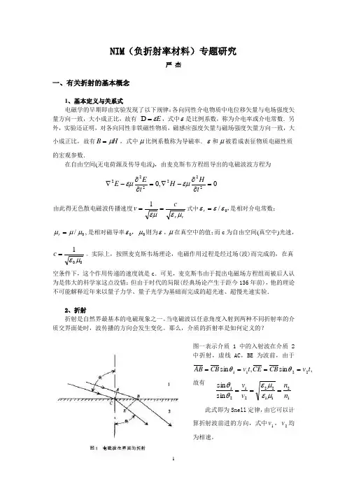
NIM （负折射率材料）专题研究严 杰一、有关折射的基本概念1、基本定义与关系式电磁学的早期即由实验发现了以下规律：各向同性介电物质中电位移矢量与电场强度矢量方向一致，大小成正比，故有 E ε=D ，式中ε是比例系数，称为介电率或介电常数．另外，实验还证明，对各向同性非铁磁性物质，磁感应强度矢量与磁场强度矢量方向一致，大小成正比，故有H B μ=，式中μ比例系数称为导磁率．ε和μ被看成表征物质电磁性质的宏观参数．在自由空间(无电荷源及传导电流)，由麦克斯韦方程组导出的电磁波波方程为由此得无色散电磁波传播速度rr cv μεεμ==1式中，0/εεε=r 是相对介电常数；,/0μμμ=r 是相对磁导率00με，则为ε，μ在真空中的值；而c 为自由空间(真空中)光速，001με=c 。

实际上，按照麦克斯韦场理论，电磁作用过程是经过场(波)而完成的，在真空条件下，这个作用传递的速度就是c ．可见，麦克斯韦由于提出电磁场方程组而被后人认为是伟大的科学家这点没错；但由于时代的局限(经典场论产生于距今136年前)，他的理论不可能解释近年来以量子力学、量子光学为基础而完成的超光速、超慢光速实验．2、折射折射是自然界最基本的电磁现象之一。

当电磁波以任意角度入射到两种不同折射率的介质交界面处时，波传播的方向会发生变化。

那么，介质的折射率是如何定义的？图一表示介质1中的入射波在介质2中折射，虚线AC ，BE 为波前，由于,sin ,sin 2211t v CB CE t v CB AB ====θθ故有此式即为Snell 定律，由它可以计算折射波前进的方向，式中1v ，2v 均为相速。

0,0222222=∂∂-∇=∂∂-∇t H H t E E εμεμ1211222121sin sin n n v v ===μεμεθθ这个比值被称为折射率，用n 表示，1122μεμε=n ，如0101,μμεε==，（介质1为真空），μμεε==22,，，则有r r vcn με==。

洛伦茨吸引子维基百科，自由的百科全书跳转到：导航，搜索ρ=28、σ=10、β=8/3时的洛伦兹系统轨迹洛伦茨吸引子是洛伦茨振子（Lorenz oscillator）的长期行为对应的分形结构，以爱德华·诺顿·洛伦茨的姓氏命名。

洛伦茨振子是能产生混沌流的三维动力系统，以其双纽线形状而著称。

映射展示出动力系统（三维系统的三个变量）的状态是如何以一种复杂且不重复的模式，随时间的推移而演变的。

目录[隐藏]1 简述2 洛伦茨方程3 瑞利数4 源代码 4.1 GNU Octave4.2 Borland C4.3 Borland Pascal4.4 Fortran4.5QBASIC/FreeBASIC("fbc -lang qb")5 参见 6 参考文献7 外部链接简述洛伦茨方程的一条轨迹被描绘成金属线，以展现方向以及三维结构洛伦茨吸引子及其导出的方程组是由爱德华·诺顿·洛伦茨于1963年发表，最初是发表在《大气科学杂志》（Journal of the Atmospheric Sciences）杂志的论文《Deterministic Nonperiodic Flow》中提出的，是由大气方程中出现的对流卷方程简化得到的。

这一洛伦茨模型不只对非线性数学有重要性，对于气候和天气预报来说也有着重要的含义。

行星和恒星大气可能会表现出多种不同的准周期状态，这些准周期状态虽然是完全确定的，但却容易发生突变，看起来似乎是随机变化的，而模型对此现象有明确的表述。

从技术角度看来，洛伦茨振子具有非线性、三维性和确定性。

2001年，沃里克·塔克尔（Warwick Tucker）证明出在一组确定的参数下，系统会表现出混沌行为，显示出人们今天所知的奇异吸引子。

这样的奇异吸引子是豪斯多夫维数在2与3之间的分形。

彼得·格拉斯伯格（Peter Grassberger）已于1983年估算出豪斯多夫维数为2.06 ±0.01，而关联维数为2.05 ±0.01。

Derivation of the Lorentz Force Law and the Magnetic Field Concept using an Invariant Formulation of the LorentzTransformationJ.H.FieldD´e partement de Physique Nucl´e aire et Corpusculaire Universit´e de Gen`e ve.24,quaiErnest-Ansermet CH-1211Gen`e ve4.e-mail;john.field@cern.chAbstractIt is demonstrated how the right hand sides of the Lorentz Transformation equa-tions may be written,in a Lorentz invariant manner,as4–vector scalar products.The formalism is shown to provide a short derivation,in which the4–vector elec-tromagnetic potential plays a crucial role,of the Lorentz force law of classical elec-trodynamics,and the conventional definition of the magneticfield in terms spatialderivatives of the4–vector potential.The time component of the relativistic gen-eralisation of the Lorentz force law is discussed.An important physical distinctionbetween the space-time and energy-momentum4–vectors is also pointed out.Keywords;Special Relativity,Classical Electrodynamics.PACS03.30+p03.50.De1IntroductionNumerous examples exist in the literature of the derivation of electrodynamical equa-tions from simpler physical hypotheses.In Einstein’s original paper on Special Relativ-ity[1],the Lorentz force law was derived by performing a Lorentz transformation of the electromagneticfields and the space-time coordinates from the rest frame of an electron (where only electrostatic forces act)to the laboratory system where the electron is in motion and so also subjected to magnetic forces.A similar demonstration was given by Schwartz[2]who also showed how the electrodynamical Maxwell equations can be derived from the Gauss laws of electrostatics and magnetostatics by exploiting the4-vector char-acter of the electromagnetic current and the symmetry properties of the electromagnetic field tensor.The same type of derivation of electrodynamic Maxwell equations from the electrostatic and magnetostatic ones has recently been performed by the present author on the basis of‘space-time exchange symmetry’[3].Frisch and Wilets[4]discussed the derivation of Maxwell’s equations and the Lorentz force law by application of relativistic transforms to the electrostatic Gauss law.Dyson[5]published a proof,due originally to Feynman,of the Faraday-Lenz law of induction,based on Newton’s Second Law and the quantum commutation relations of position and momentum,that excited considerable interest and aflurry of comments and publications[6,7,8,9,10,11]about a decade ndau and Lifshitz[12]presented a derivation of Amp`e re’s Law from the electro-dynamic Lagrangian,using the Principle of Least Action.By relativistic transformation of the Coulomb force from the rest frame of a charge to another inertial system in rela-tive motion,Lorrain,Corson and Lorrain[13]derived both the Biot-Savart law,for the magneticfield generated by a moving charge,and the Lorentz force law.In many text books on classical electrodynamics the question of what are the funda-mental physical hypotheses underlying the subject,as distinct from purely mathematical developments of these hypotheses,used to derive predictions,is not discussed in any de-tail.Indeed,it may even be stated that it is futile to address the question at all.For example,Jackson[14]states:At present it is popular in undergraduate texts and elsewhere to attempt to derive magneticfields and even Maxwell equations from Coulomb’s law of electrostatics and the theory of Special Relativity.It should immediately obvious that,without additional assumptions,this is impossible.’This is,perhaps,a true statement.However,if the additional assumptions are weak ones,the derivation may still be a worthwhile exercise.In fact,in the case of Maxwell’s equations,as shown in References[2,3],the‘additional assumptions’are merely the formal definitions of the electric and magneticfields in terms of the space–time derivatives of the 4–vector potential[15].In the case of the derivation of the Lorentz force equation given below,not even the latter assumption is required,as the magneticfield definition appears naturally in the course of the derivation.In the chapter on‘The Electromagnetic Field’in Misner Thorne and Wheeler’s book ‘Gravitation’[16]can be found the following statement:Here and elsewhere in science,as stressed not least by Henri Poincar´e,that view isout of date which used to say,“Define your terms before you proceed”.All the laws and theories of physics,including the Lorentz force law,have this deep and subtle chracter, that they both define the concepts they use(here B and E)and make statements about these concepts.Contrariwise,the absence of some body of theory,law and principle deprives one of the means properly to define or even use concepts.Any forward step in human knowlege is truly creative in this sense:that theory concept,law,and measurement —forever inseperable—are born into the world in union.I do not agree that the electric and magneticfields are the fundamental concepts of electromagnetism,or that the Lorentz force law cannot be derived from simpler and more fundamental concepts,but must be‘swallowed whole’,as this passage suggests. As demonstrated in References[2,3]where the electrodynamic and magnetodynamic Maxwell equations are derived from those of electrostatics and magnetostatics,a more economical description of classical electromagentism is provided by the4–vector potential. Another example of this is provided by the derivation of the Lorentz force law presented in the present paper.The discussion of electrodynamics in Reference[16]is couched entirely in terms of the electromagneticfield tensor,Fµν,and the electric and magnetic fields which,like the Lorentz force law and Maxwell’s equations,are‘parachuted’into the exposition without any proof or any discussion of their interrelatedness.The4–vector potential is introduced only in the next-but-last exercise at the end of the chapter.After the derivation of the Lorentz force law in Section3below,a comparison will be made with the treatment of the law in References[2,14,16].The present paper introduces,in the following Section,the idea of an‘invariant for-mulation’of the Lorentz Transformation(LT)[17].It will be shown that the RHS of the LT equations of space and time can be written as4-vector scalar products,so that the transformed4-vector components are themselves Lorentz invariant quantities.Consid-eration of particular length and time interval measurements demonstrates that this is a physically meaningful concept.It is pointed out that,whereas space and time intervals are,in general,physically independent physical quantities,this is not the case for the space and time components of the energy-momentum4-vector.In Section3,a derivation of the Lorentz force law,and the associated magneticfield concept,is given,based on the invariant formulation of the LT.The derivation is very short,the only initial hypothesis being the usual definition of the electricfield in terms of the4-vector potential,which,in fact,is also uniquely specified by requiring the definition to be a covariant one.In Section 4the time component of Newton’s Second Law in electrodynamics,obtained by applying space-time exchange symmetry[3]to the Lorentz force law,is discussed.Throughout this paper it is assumed that the electromagneticfield constitutes,to-gether with the moving charge,a conservative system;i.e.effects of radiation,due to the acceleration of the charge,are neglected2Invariant Formulation of the Lorentz Transforma-tionThe space-time LT equations between two inertial frames S and S’,written in a space-time symmetric manner,are:x =γ(x−βx0)(2.1)y =y(2.2)z =z(2.3)x 0=γ(x0−βx)(2.4) The frame S’moves with velocity,v,relative to S,along the common x-axis of S and S’.βandγare the usual relativistic parameters:vβ≡√−(∆x0)2+∆x2=∆x(2.12) since,for the measurement procedure just described,∆x0=0.Notice that∆x is not necessarily defined in terms of such a measurement.If,following Einstein[1],the interval ∆x is associated with the length, ,of a measuring rod at rest in S and lying parallel to the x-axis,measurements of the ends of the rod can be made at arbitarily different times in S.The same result =∆x will be found for the length of the rod,but the corresponding invariant interval,S x,as defined by Eqn(2.12)will be different in each case.Similarly,∆x0may be identified with the time-like invariant interval corresponding to successive observations of a clock at afixed position(i.e.∆x=0)in S:S0≡the same value,∆x0,for the time difference between two events in S,but with different values of the invariant interval defined by Eqn(2.13).In virtue of Eqns(2.12)and(2.13)the LT equations(2.8)and(2.11)may be written the following invariant form:S x=−¯U(β)·S(2.14)S 0=U(β)·S(2.15) where the following4–vectors have been introduced:S≡(S0;S x,0,0)=(∆x0;∆x,0,0)(2.16)U(β)≡(γ;γβ,0,0)(2.17)¯U(β)≡(γβ;γ,0,0)(2.18)The time-like4-vector,U,is equal to V/c,where V is the usual4–vector velocity,whereas the space-like4–vector,¯U,is‘orthogonal to U in four dimensions’:U(β)·¯U(β)=0(2.19) Since the RHS of(2.14)and(2.15)are4–vector scalar products,S x and S 0are manifestly Lorentz invariant quantites.These4–vector components may be defined,in terms of specific space-time measurements,by equations similar to(2.12)and(2.13)in the frame S’.Note that the4–vectors S and S are‘doubly covariant’in the sense that S·S and S ·S are‘doubly invariant’quantities whose spatial and temporal terms are,individually, Lorentz invariant:S·S=S20−S2x=S ·S =(S 0)2−(S x)2(2.20) Every term in Eqn(2.20)remains invariant if the spatial and temporal intervals described above are observed from a third inertial frame S”moving along the x-axis relative to both S and S’.This follows from the manifest Lorentz invariance of the RHS of Eqn(2.14)and (2.15)and their inverses:S x=−¯U(−β)·S (2.21)S0=U(−β)·S (2.22) Since the LT Eqns(2.1)and(2.4)are valid for any4–vector,W,it follows that:W x=−¯U(β)·W(2.23)W 0=U(β)·W(2.24) Again,W x and W 0are manifestly Lorentz invariant.An interesting special case is the energy-momentum4–vector,P,of a physical object of mass,m.Here the‘doubly in-variant’quantity analagous to S·S in Eqn(2.20)is equal to m2c2.Choosing the x-axis parallel to p andβto correspond to the object’s velocity,so that S’is the object’s proper frame,and since P≡mcU(β),Eqns(2.23)and(2.24)yield,for this special case:P x=−mc¯U(β)·U(β)=0(2.25)P 0=mcU(β)·U(β)=mc(2.26)Since the Lorentz transformation is determined by the single parameter,β,then it follows from Eqns(2.25)and(2.26)that,unlike in the case of the space and time intervals in Eqns(2.8)and(2.11),the spatial and temporal components of the energy momentum 4–vector,in an arbitary inertial frame,are not independent.In fact,P0is determined in terms of P x and m by the relation,that follows from the inverse of Eqns(2.25)and(2.26):P0=Thus,from rotational invariance,the general covariant definition of the electricfield is:E i=∂i A0−∂0A i(3.4) This is the‘additional assumption’,mentioned by Jackson in the passage quoted above, that is necessary,in the present case,to derive the Lorentz force law.However,as written, it concerns only the physical properties of the electricfield:the magneticfield concept has not yet been introduced.A further a posteriori justification of Eqn(3.4)will be given after derivation of the Lorentz force law.Here it is simply noted that,if the spatial part of the4–vector potential is time-independent,Eqn(3.4)reduces to the usual electrostatic definition of the electricfield.The force F on an electric charge q at rest in the frame S’is given by the definition of the electricfield,and Eqn(3.4)as:F i=q(∂ i A 0−∂ 0A i)(3.5) Equations analagous to(2.24)may be written relating A and∂ to the corresponding quantities in the frame S moving along the x’axis with velocity−v relative to S’:∂ 0=U(β)·∂(3.6)A 0=U(β)·A(3.7) Substituting(3.6)and(3.7)in(3.5)gives:F i=q∂ i(U(β)·A)−(U(β)·∂)A i(3.8)This equation expresses a linear relationship between F i,∂ i and A i.Since the coefficients of the relation are Lorentz invariant,the same formula is valid in any inertial frame,in particular,in the frame S.Hence:F i=q∂i(U(β)·A)−(U(β)·∂)A i(3.9)This equation gives,in4–vector notation,a spatial component of the Lorentz force on the charge q in the frame S,and so completes the derivation.To express the Lorentz force formula in the more familiar3-vector notation,it is convenient to introduce the relativistic generalisation of Newton’s Second Law[19]:dPdτ=γdP iIntroducing now the magneticfield according to the definition[20]:B k≡− ijk(∂i A j−∂j A i)=( ∇× A)k(3.12) enables Eqn(3.11)to be written in the compact form:dP idγ βt=mc(3.15)∂twhere Eqn(3.12)has been used.Eqn(3.15)is just the Faraday-Lenz induction law,i.e.the magnetodynamic Maxwell equation.This is only apparent,however,once the‘magnetic field’concept of Eqn(3.12)has been introduced.Thus the initial hypothesis,Eqn(3.4),is actually a Maxwell equation.This is the a posteriori justification,mentioned above,for this covariant definition of the electricfield.It is common in discussions of electromagnetism to introduce the second rank electro-magneticfield tensor,Fµνaccording to the definition:Fµν≡∂µAν−∂νAµ(3.16) in terms of which,the electric and magneticfields are defined as:E i≡F i0(3.17)B k≡− ijk F ij(3.18) From the point of view adopted in the present paper both the electromagneticfield tensor and the electric and magneticfields themselves are auxiliary quantities introduced only for mathematical convenience,in order to write the equations of electromagnetism in a compact way.Since all these quantities are completly defined by the4–vector potential, it is the latter quantity that encodes all the relevant physical information on any electro-dynamic problem[21].This position is contrary to that commonly taken in the literature and texbooks where it is often claimed that only the electric and magneticfields have physical significance,while the4–vector potential is only a convenient mathematical tool. For example R¨o hrlich[22]makes the statement:These functions(φand A)known as potentialsmanner!In other cases(e.g.Maxwell’s equations)simpler expessions may be written interms of the4–vector potential.The quantum theory,quantum electrodynamics,thatunderlies classical electromagnetism,requires the introduction the4–vector photonfield Aµin order to specify the minimal interaction that provides the dynamical basis of the theory.Similarly,the introduction of Aµis necessary for the Lagrangian formulation ofclassical electromagnetism.It makes no sense,therefore,to argue that a physical conceptof such fundamental importance has‘no physical meaning’.The initial postulate used here to derive the Lorentz force law is Eqn(3.4),whichcontains,explicitly,the electrostatic force law and,implicitly,the Faraday-Lenz inductionlaw.The actual form of the electrostatic force law(Coulomb’s inverse square law)is notinvoked,suggesting that the Lorentz force law may be of greater generality.On theassumption of Eqn(3.4)(which has been demonstrated to be the only possible covariantdefinition of the electricfield),the existence of the‘magneticfield’,the‘electromagneticfield tensor’,andfinally the Lorentz force law itself have all been derived,without furtherassumptions,by use of the invariant formulation of the Lorentz transformation.It is instructive to compare the derivation of the Lorentz force law given in the presentpaper with that of Reference[13]based on the relativistic transformation properties of theCoulomb force3–vector.Coulomb’s law is not used in the present paper.On the otherhand,Reference[13]makes no use of the4–vector potential concept,which is essential forthe derivation presented here.This demonstrates an interesting redundancy among thefundamental physical concepts of classical electromagnetism.In Reference[2],Eqns(3.4),(3.12)and(3.16)were all introduced as a priori initialpostulates without further justification.In fact,Schwartz gave the following explanationfor his introduction of Eqn(3.16)[23]:So far everything we have done has been entirely deductive,making use only ofCoulomb’s law,conservation of charge under Lorentz transformation and Lorentz in-variance for our physical laws.We have now come to the end of this deductive path.Atthis point when the laws were being written,God had to make a decision.In generalthere are16components of a second-rank tensor in four dimensions.However,in anal-ogy to three dimensions we can make a major simplification by choosing the completelyantisymmetric tensor to represent ourfield quantities.Then we would have only6inde-pendent components instead of the possible16.Under Lorentz transformation the tensorwould remain antisymmetric and we would never have need for more than six independentcomponents.Appreciating this,and having a deep aversion to useless complication,Godnaturally chose the antsymmetric tensor as His medium of expression.Actually it is possible that God may have previously invented the4–vector potentialand special relativity,which lead,as shown above,to Eqn(3.4)as the only possible co-variant definition of the electricfield.As also shown in the present paper,the existence ofthe remaining elements of the antisymmetricfield tensor,containing the magneticfield,then follow from special relativity alone.Schwartz derived the Lorentz force law,as inEinstein’s original Special Relativity paper[1],by Lorentz transformation of the electricfield,from the rest frame of the test charge,to one in which it is in motion.This requiresthat the magneticfield concept has previously been introduced as well as knowledge ofthe Lorentz transformation laws of the electric and magneticfields.In the chapter devoted to special relativity in Jackson’s book[24]the Lorentz forcelaw is simply stated,without any derivation,as are also the defining equations of theelectric and magneticfields and the electromagneticfield tensor just mentioned.Noemphasis is therefore placed on the fundamental importance of the4–vector potential inthe relativistic description of electromagnetism.In order to treat,in a similar manner,the electromagnetic and gravitationalfields,thediscussion in Misner Thorne and Wheeler[16]is largely centered on the properties of thetensor Fµν.Again the Lorentz force equation is introduced,in the spirit of the passagequoted above,without any derivation or discussion of its meaning.The defining equationsof the electric and magneticfields and Fµν,in terms of Aµ,appear only in the eighteenthexercise of the relevant chapter.The main contents of the chapter on the electromagneticfield are an extended discussion of purely mathematical tensor manipulations that obscurethe essential simplicity of electromagnetism when formulated in terms of the4–vectorpotential.In contrast to References[2,24,16],in the derivation of the Lorentz force law andthe magneticfield presented here,the only initial assumption,apart from the validityof special relativity,is the chosen definition,Eqn(3.4),of the electricfield in terms ofthe4–vector potential Aµ,which is the only covariant one.Thus,a more fundamentaldescription of electromagnetism than that provided by the electric and magneticfieldconcepts is indeed possible,contrary to the opinion expressed in the passage from MisnerThorne and Wheeler quoted above.4The time component of Newton’s Second Law in ElectrodynamicsSpace-time exchange symmetry[3]states that physical laws inflat space are invariantwith respect to the exchange of the space and time components of4-vectors.For example,the LT of time,Eqn(2.4),is obtained from that for space,Eqn(2.1),by applying the space-time exchange(STE)operations:x0↔x,x 0↔x .In the present case,application of the STE operation to the spatial component of the Lorentz force equation in the secondline of Eqn(3.11)leads to the relation:dP00(4.1)where Eqns(2.5)and(3.4)and the following properties of the STE operation[3]have been used:∂0↔−∂i(4.2)A0↔−A i(4.3)C·D↔−C·D(4.4)Eqn(4.1)yields an expression for the time derivative of the relativistic energy,E=P0:d E(4.5)Integration of Eqn(4.5)gives the equation of energy conservation for a particle moving from an initial position, x I,to afinal position, x F,under the influence of electromagnetic forces:E F E I d E=qxFx IE·d x(4.6)Thus work is done on the moving charge only by the electricfield.This is also evident from the Lorentz force equation,(3.14),since the magnetic force β× B is perpendicular to the velocity vector,so that no work is performed by the magneticfield.A corollary is that the relativistic energy(and hence the magnitude of the velocity)of a charged particle moving in a constant magneticfield is a constant of the motion.Of course,Eqn(4.5) may also be derived directly from the Lorentz force law,so that the time component of the relativistic generalisation of Newton’s Second Law,Eqn(4.1),contains no physical information not already contained in the spatial components.This is related to the fact that,as demonstrated in Eqns(2.25)and(2.26),the spatial and temporal components of the energy-momentum4–vector are not independent physical quantities.AcknowledgementsI should like to thank O.L.de Lange for asking the question whose answer,presented in Section4,was the original motivation for the writing of this paper,and an anonymous referee of an earlier version of this paper for informing me of related material,in the books of Jackson and Misner,Thorne and Wheeler,which is discussed in some detail in this version.References[1]A.Einstein,17891(1905).[2]M.Schwartz,‘Principles of Electrodynamics’,(McGraw-Hill,New York,1972)Ch3.[3]J.H.Field,Am.J.Phys.69569(2001).[4]D.H.Frisch and L.Wilets,Am.J.Phys.24574(1956).[5]F.J.Dyson,Am.J.Phys.58209(1990).[6]N.Dombey,Am.J.Phys.5985(1991).[7]R.W.Breheme,Am.J.Phys.5985(1991).[8]J.L.Anderson,Am.J.Phys.5986(1991).[9]I.E.Farquhar,Am.J.Phys.5987(1991).[10]S.Tanimura,Ann.Phys.(N.Y.)220229(1992).[11]A.Vaidya and C.Farina,Phys.Lett.153A265(1991).[12]ndau and E.M.Lifshitz,‘The Classical Theory of Fields’,(Pergamon Press,Oxford,1975)Section30,P93.[13]P.Lorrain, D.R.Corson and F.Lorrain,‘Electromagnetic Fields and Waves’,(W.H.Freeman,New York,Third Edition,1988)Section16.5,P291.[14]J.D.Jackson,‘Classical Electrodynamics’,(John Wiley and Sons,New York,1975)Section12.2,P578.[15]Actually,a careful examination of the derivation of Amp`e re’s from the Gauss lawof electrostatics in Reference[3]shows that,although Eqn(3.4)of the present paper is a necessary initial assumption,the definition of the magneticfield in terms of the spatial derivatives of the4–vector potential occurs naturally in the course of the derivation(see Eqns(5.16)and(5.17)of Reference[3])so it is not necessary to assume, at the outset,the expression for the spatial components of the electromagneticfield tensor as given by Eqn(5.1)of Reference[3].[16]C.W.Misner,K.S.Thorne and J.A.Wheeler,‘Gravitation’,(W.H.Freeman,San Fran-cisco,1973)Ch3,P71.[17]This should not be confused with a manifestly covariant expression for the LT,whereit is written as a linear4-vector relation with Lorentz-invariant coefficients,as in:D.E.Fahnline,Am.J.Phys.50818(1982).[18]A time-like metric is used for4-vector products with the components of a4–vector,W,defined as:W t=W0=W0,W x,y,z=W1,2,3=−W1,2,3and an implied summation over repeated contravariant(upper)and covariant(lower) indices.Repeated Greek indices are summed from0to3,repeated Roman ones from1to3.Also∂µ≡(∂∂x1,−∂∂x3)=(∂0;− ∇)[19]H.Goldstein,‘Classical Mechanics’,(Addison-Wesley,Reading Massachusetts,1959)P200,Eqn(6-30).[20]The alternating tensor, ijk,equals1(−1)for even(odd)permutations of ijk.[21]The explicit form of Aµ,as derived from Coulomb’s law,is given in standard text-books on classical electrodynamics.For example,in Reference[13],it is to be found in Eqns(17-51)and(17-52).Aµis actually proportional to the4-vector velocity,V, of the charged particle that is the source of the electromagneticfield.[22]F.R¨o hrlich,‘Classical Charged Particles’,(Addison-Wesley,Reading,MA,1990)P65.[23]Reference[2]above,Ch3,P127.[24]Reference[14]above,Section11.9,P547.。