Laser Guide Star Adaptive Optics Integral Field Spectroscopy of a Tightly Collimated Bipola
- 格式:pdf
- 大小:610.87 KB
- 文档页数:11

《光电技术》专业英语词汇1.Absorption coefficient 吸收系数2.Acceptance angle 接收角3.fibers 光纤4.Acceptors in semiconductors 半导体接收器5.Acousto-optic modulator 声光调制6.Bragg diffraction 布拉格衍射7.Air disk 艾里斑8.angular radius 角半径9.Airy rings 艾里环10.anisotropy 各向异性11.optical 光学的12.refractive index 各向异性13.Antireflection coating 抗反膜14.Argon-ion laser 氩离子激光器15.Attenuation coefficient 衰减系数16.Avalanche 雪崩17.breakdown voltage 击穿电压18.multiplication factor 倍增因子19.noise 燥声20.Avalanche photodiode(APD) 雪崩二极管21.absorption region in APD APD 吸收区域22.characteristics-table 特性表格23.guard ring 保护环24.internal gain 内增益25.noise 噪声26.photogeneration 光子再生27.primary photocurrent 起始光电流28.principle 原理29.responsivity of InGaAs InGaAs 响应度30.separate absorption and multiplication(SAM) 分离吸收和倍增31.separate absorption grading and multiplication(SAGM) 分离吸收等级和倍增32.silicon 硅33.Average irradiance 平均照度34.Bandgap 带隙35.energy gap 能级带隙36.bandgap diagram 带隙图37.Bandwidth 带宽38.Beam 光束39.Beam splitter cube 立方分束器40.Biaxial crystal双s 轴晶体41.Birefringent 双折射42.Bit rate 位率43.Black body radiation law 黑体辐射法则44.Bloch wave in a crystal 晶体中布洛赫波45.Boundary conditions 边界条件46.Bragg angle 布拉格角度47.Bragg diffraction condition 布拉格衍射条件48.Bragg wavelength 布拉格波长49.Brewster angle 布鲁斯特角50.Brewster window 布鲁斯特窗51.Calcite 霰石52.Carrier confinement 载流子限制53.Centrosymmetric crystals 中心对称晶体54.Chirping 啁啾55.Cladding 覆层56.Coefficient of index grating 指数光栅系数57.Coherence连贯性pensation doping 掺杂补偿59.Conduction band 导带60.Conductivity 导电性61.Confining layers 限制层62.Conjugate image 共轭像63.Cut-off wavelength 截止波长64.Degenerate semiconductor 简并半导体65.Density of states 态密度66.Depletion layer 耗尽层67.Detectivity 探测率68.Dielectric mirrors 介电质镜像69.Diffraction 衍射70.Diffraction g rating 衍射光栅71.Diffraction grating equation 衍射光栅等式72.Diffusion current 扩散电流73.Diffusion flux 扩散流量74.Diffusion Length 扩散长度75.Diode equation 二极管公式76.Diode ideality factor 二极管理想因子77.Direct recombinatio直n接复合78.Dispersion散射79.Dispersive medium 散射介质80.Distributed Bragg reflector 分布布拉格反射器81.Donors in semiconductors 施主离子82.Doppler broadened linewidth 多普勒扩展线宽83.Doppler effect 多普勒效应84.Doppler shift 多普勒位移85.Doppler-heterostructure 多普勒同质结构86.Drift mobility 漂移迁移率87.Drift Velocity 漂移速度88.Effective d ensity o f s tates 有效态密度89.Effective mass 有效质量90.Efficiency 效率91.Einstein coefficients 爱因斯坦系数92.Electrical bandwidth of fibers 光纤电子带宽93.Electromagnetic wave 电磁波94.Electron affinity 电子亲和势95.Electron potential energy in a crystal 晶体电子阱能量96.Electro-optic effects 光电子效应97.Energy band 能量带宽98.Energy band diagram 能量带宽图99.Energy level 能级100.E pitaxial growth 外延生长101.E rbium doped fiber amplifier 掺饵光纤放大器102.Excess carrier distribution 过剩载流子扩散103.External photocurrent 外部光电流104.Extrinsic semiconductors 本征半导体105.Fabry-Perot laser amplifier 法布里-珀罗激光放大器106.Fabry-Perot optical resonator 法布里-珀罗光谐振器107.Faraday effect 法拉第效应108.Fermi-Dirac function 费米狄拉克结109.Fermi energy 费米能级110.Fill factor 填充因子111.Free spectral range 自由谱范围112.Fresnel’s equations 菲涅耳方程113.Fresnel’s optical indicatrix 菲涅耳椭圆球114.Full width at half maximum 半峰宽115.Full width at half power 半功率带宽116.Gaussian beam 高斯光束117.Gaussian dispersion 高斯散射118.Gaussian pulse 高斯脉冲119.Glass perform 玻璃预制棒120.Goos Haenchen phase shift Goos Haenchen 相位移121.Graded index rod lens 梯度折射率棒透镜122.Group delay 群延迟123.Group velocity 群参数124.Half-wave plate retarder 半波延迟器125.Helium-Neon laser 氦氖激光器126.Heterojunction 异质结127.Heterostructure 异质结构128.Hole 空穴129.Hologram 全息图130.Holography 全息照相131.Homojunction 同质结132.Huygens-Fresnel principle 惠更斯-菲涅耳原理133.Impact-ionization 碰撞电离134.Index matching 指数匹配135.Injection 注射136.Instantaneous irradiance 自发辐射137.Integrated optics 集成光路138.Intensity of light 光强139.Intersymbol interference 符号间干扰140.Intrinsic concentration 本征浓度141.Intrinsic semiconductors 本征半导体142.Irradiance 辐射SER 激光144.active medium 活动介质145.active region 活动区域146.amplifiers 放大器147.cleaved-coupled-cavity 解理耦合腔148.distributed Bragg reflection 分布布拉格反射149.distributed feedback 分布反馈150.efficiency of the He-Ne 氦氖效率151.multiple quantum well 多量子阱152.oscillation condition 振荡条件ser diode 激光二极管sing emission 激光发射155.LED 发光二极管156.Lineshape function 线形结157.Linewidth 线宽158.Lithium niobate 铌酸锂159.Load line 负载线160.Loss c oefficient 损耗系数161.Mazh-Zehnder modulator Mazh-Zehnder 型调制器162.Macrobending loss 宏弯损耗163.Magneto-optic effects 磁光效应164.Magneto-optic isolator 磁光隔离165.Magneto-optic modulator 磁光调制166.Majority carriers 多数载流子167.Matrix emitter 矩阵发射168.Maximum acceptance angle 最优接收角169.Maxwell’s wave equation 麦克斯维方程170.Microbending loss 微弯损耗171.Microlaser 微型激光172.Minority carriers 少数载流子173.Modulated directional coupler 调制定向偶合器174.Modulation of light 光调制175.Monochromatic wave 单色光176.Multiplication region 倍增区177.Negative absolute temperature 负温度系数 round-trip optical gain 环路净光增益179.Noise 噪声180.Noncentrosymmetric crystals 非中心对称晶体181.Nondegenerate semiconductors 非简并半异体182.Non-linear optic 非线性光学183.Non-thermal equilibrium 非热平衡184.Normalized frequency 归一化频率185.Normalized index difference 归一化指数差异186.Normalized propagation constant 归一化传播常数187.Normalized thickness 归一化厚度188.Numerical aperture 孔径189.Optic axis 光轴190.Optical activity 光活性191.Optical anisotropy 光各向异性192.Optical bandwidth 光带宽193.Optical cavity 光腔194.Optical divergence 光发散195.Optic fibers 光纤196.Optical fiber amplifier 光纤放大器197.Optical field 光场198.Optical gain 光增益199.Optical indicatrix 光随圆球200.Optical isolater 光隔离器201.Optical Laser amplifiers 激光放大器202.Optical modulators 光调制器203.Optical pumping 光泵浦204.Opticalresonator 光谐振器205.Optical tunneling光学通道206.Optical isotropic 光学各向同性的207.Outside vapor deposition 管外气相淀积208.Penetration depth 渗透深度209.Phase change 相位改变210.Phase condition in lasers 激光相条件211.Phase matching 相位匹配212.Phase matching angle 相位匹配角213.Phase mismatch 相位失配214.Phase modulation 相位调制215.Phase modulator 相位调制器216.Phase of a wave 波相217.Phase velocity 相速218.Phonon 光子219.Photoconductive detector 光导探测器220.Photoconductive gain 光导增益221.Photoconductivity 光导性222.Photocurrent 光电流223.Photodetector 光探测器224.Photodiode 光电二极管225.Photoelastic effect 光弹效应226.Photogeneration 光子再生227.Photon amplification 光子放大228.Photon confinement 光子限制229.Photortansistor 光电三极管230.Photovoltaic devices 光伏器件231.Piezoelectric effect 压电效应232.Planck’s radiation distribution law 普朗克辐射法则233.Pockels cell modulator 普克尔斯调制器234.Pockel coefficients 普克尔斯系数235.Pockels phase modulator 普克尔斯相位调制器236.Polarization 极化237.Polarization transmission matrix 极化传输矩阵238.Population inversion 粒子数反转239.Poynting vector 能流密度向量240.Preform 预制棒241.Propagation constant 传播常数242.Pumping 泵浦243.Pyroelectric detectors 热释电探测器244.Quantum e fficiency 量子效应245.Quantum noise 量子噪声246.Quantum well 量子阱247.Quarter-wave plate retarder 四分之一波长延迟248.Radiant sensitivity 辐射敏感性249.Ramo’s theorem 拉莫定理250.Rate equations 速率方程251.Rayleigh criterion 瑞利条件252.Rayleigh scattering limit 瑞利散射极限253.Real image 实像254.Recombination 复合255.Recombination lifetime 复合寿命256.Reflectance 反射257.Reflection 反射258.Refracted light 折射光259.Refractive index 折射系数260.Resolving power 分辩力261.Response time 响应时间262.Return-to-zero data rate 归零码263.Rise time 上升时间264.Saturation drift velocity 饱和漂移速度265.Scattering 散射266.Second harmonic generation 二阶谐波267.Self-phase modulation 自相位调制268.Sellmeier dispersion equation 色列米尔波散方程式269.Shockley equation 肖克利公式270.Shot noise 肖特基噪声271.Signal to noise ratio 信噪比272.Single frequency lasers 单波长噪声273.Single quantum well 单量子阱274.Snell’s law 斯涅尔定律275.Solar cell 光电池276.Solid state photomultiplier 固态光复用器277.Spectral intensity 谱强度278.Spectral responsivity 光谱响应279.Spontaneous emission 自发辐射280.stimulated emission 受激辐射281.Terrestrial light 陆地光282.Theraml equilibrium 热平衡283.Thermal generation 热再生284.Thermal velocity 热速度285.Thershold concentration 光强阈值286.Threshold current 阈值电流287.Threshold wavelength 阈值波长288.Total acceptance angle 全接受角289.Totla internal reflection 全反射290.Transfer distance 转移距离291.Transit time 渡越时间292.Transmission coefficient 传输系数293.Tramsmittance 传输294.Transverse electric field 电横波场295.Tranverse magnetic field 磁横波场296.Traveling vave lase 行波激光器297.Uniaxial crystals 单轴晶体298.UnPolarized light 非极化光299.Wave 波300.W ave equation 波公式301.Wavefront 波前302.Waveguide 波导303.Wave n umber 波数304.Wave p acket 波包络305.Wavevector 波矢量306.Dark current 暗电流307.Saturation signal 饱和信号量308.Fringing field drift 边缘电场漂移plementary color 补色310.Image lag 残像311.Charge handling capability 操作电荷量312.Luminous quantity 测光量313.Pixel signal interpolating 插值处理314.Field integration 场读出方式315.Vertical CCD 垂直CCD316.Vertical overflow drain 垂直溢出漏极317.Conduction band 导带318.Charge coupled device 电荷耦合组件319.Electronic shutter 电子快门320.Dynamic range 动态范围321.Temporal resolution 动态分辨率322.Majority carrier 多数载流子323.Amorphous silicon photoconversion layer 非晶硅存储型324.Floating diffusion amplifier 浮置扩散放大器325.Floating gate amplifier 浮置栅极放大器326.Radiant quantity 辐射剂量327.Blooming 高光溢出328.High frame rate readout mode 高速读出模式329.Interlace scan 隔行扫描330.Fixed pattern noise 固定图形噪声331.Photodiode 光电二极管332.Iconoscope 光电摄像管333.Photolelctric effect 光电效应334.Spectral response 光谱响应335.Interline transfer CCD 行间转移型CCD336.Depletion layer 耗尽层plementary metal oxide semi-conductor 互补金属氧化物半导体338.Fundamental absorption edge 基本吸收带339.Valence band 价带340.Transistor 晶体管341.Visible light 可见光342.Spatial filter 空间滤波器343.Block access 块存取344.Pupil compensation 快门校正345.Diffusion current 扩散电流346.Discrete cosine transform 离散余弦变换347.Luminance signal 高度信号348.Quantum efficiency 量子效率349.Smear 漏光350.Edge enhancement 轮廓校正351.Nyquist frequency 奈奎斯特频率352.Energy band 能带353.Bias 偏压354.Drift current 漂移电流355.Clamp 钳位356.Global exposure 全面曝光357.Progressive scan 全像素读出方式358.Full frame CCD 全帧CCD359.Defect correction 缺陷补偿360.Thermal noise 热噪声361.Weak inversion 弱反转362.Shot noise 散粒噪声363.Chrominance difference signal 色差信号364.Colotremperature 色温365.Minority carrier 少数载流子366.Image stabilizer 手振校正367.Horizontal CCD 水平CCD368.Random noise 随机噪声369.Tunneling effect 隧道效应370.Image sensor 图像传感器371.Aliasing 伪信号372.Passive 无源373.Passive pixel sensor 无源像素传感器374.Line transfer 线转移375.Correlated double sampling 相关双采样376.Pinned photodiode 掩埋型光电二极管377.Overflow 溢出378.Effective pixel 有效像素379.Active pixel sensor 有源像素传感器380.Threshold voltage 阈值电压381.Source follower 源极跟随器382.Illuminance 照度383.Refraction index 折射率384.Frame integration 帧读出方式385.Frame interline t ransfer CCD 帧行间转移CCD 386.Frame transfer 帧转移387.Frame transfer CCD 帧转移CCD388.Non interlace 逐行扫描389.Conversion efficiency 转换效率390.Automatic gain control 自动增益控制391.Self-induced drift 自激漂移392.Minimum illumination 最低照度393.CMOS image sensor COMS 图像传感器394.MOS diode MOS 二极管395.MOS image sensor MOS 型图像传感器396.ISO sensitivity ISO 感光度。
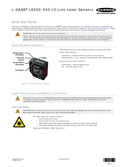
Quick Start GuideThis guide is designed to help you set up and install the L-GAGE ® LE Laser Gauging Sensor. For complete information on programming,performance, troubleshooting, dimensions, and accessories, please refer to the Instruction Manual at . Searchfor p/n 194205 to view the manual. Use of this document assumes familiarity with pertinent industry standards and practices.WARNING: Not To Be Used for Personnel ProtectionNever use this device as a sensing device for personnel protection. Doing so could lead to serious injury or death. This device does not include the self-checking redundant circuitry necessary to allow its use in personnel safety applications. A sensor failure or malfunction can cause either an energized or de-energized sensor output condition.Features and IndicatorsPower LED Indicator Discrete Output 1LED IndicatorDisplayDiscrete Output 2LED IndicatorPush ButtonsFigure 1. LE IO-Link Sensor FeaturesThree LED indicators provide ongoing indication of the sensing status.Power LED IndicatorSolid Green = Normal operation, power On and laser OnFlashing Green (1 Hz) = Power On and laser Off (laser enable mode)Discrete Output LED IndicatorsSolid Amber = Discrete Output is On Off = Discrete Output is OffLaser Description and Safety InformationCAUTION: Use of controls or adjustments or performance of procedures other than those specified herein may result in hazardous radiation exposure. Do not attempt to disassemble this sensor for repair. A defective unit must be returned to the manufacturer.Class 2 Laser ModelsCAUTION: Never stare directly into the sensor lens. Laser light can damage your eyes. Avoid placing any mirror-like object in the beam. Never use a mirror as a retroreflective target.For Safe Laser Use - Class 2 Lasers•Do not stare at the laser.•Do not point the laser at a person’s eye.•Mount open laser beam paths either above or below eye level, where practical.•Terminate the beam emitted by the laser product at the end of its useful path.Reference IEC 60825-1:2007, Section 8.2.L-GAGE ® LE250/550 IO-Link Laser SensorsOriginal Document 194204 Rev. B2 December 2016194204Class 2 LasersClass 2 lasers are lasers that emit visible radiation in the wavelength range from 400 nm to 700nm, where eye protection is normally afforded by aversion responses, including the blink reflex.This reaction may be expected to provide adequate protection under reasonably foreseeableconditions of operation, including the use of optical instruments for intrabeam viewing.Figure 2. FDA (CDRH) warning label(Class 2)Class 2 Laser Safety NotesLow-power lasers are, by definition, incapable of causing eye injury within the duration of a blink (aversion response) of 0.25 seconds. They also must emit only visible wavelengths (400 to 700nm). Therefore, an ocular hazard may exist only if individuals overcome their natural aversion to bright light and stare directly into the laser beam.Class 1 Laser ModelsClass 1 lasers are lasers that are safe under reasonably foreseeable conditions of operation,including the use of optical instruments for intrabeam viewing.Figure 3. FDA (CDRH) warning label(Class 1)Laser wavelength: 650 nmOutput: < 0.22 mWPulse Duration: 150 µs to 900 µsSensor InstallationNOTE: Handle the sensor with care during installation and operation. Sensor windows soiled by fingerprints, dust,water, oil, etc. may create stray light that may degrade the peak performance of the sensor. Blow the window clear using filtered, compressed air, then clean as necessary using 70% isopropyl alcohol and cotton swabs or water and a soft cloth.Sensor OrientationCorrect sensor-to-object orientation is important to ensure proper sensing. See the following figures for examples of correct and incorrect sensor-to-object orientation as certain placements may pose problems for sensing distances.Figure 4. Orientation by a wall IncorrectCorrectFigure 5. Orientation in an opening IncorrectCorrect Figure 6. Orientation for a turning object - Tel: +1-763-544-3164P/N 194204 Rev. BIncorrectCorrectFigure 7. Orientation for a height differenceIncorrectCorrect Figure 8. Orientation for a color or lusterdifference Figure 9. Orientation for a highly reflectivetargetApplying tilt to sensor may improve performance on reflective targets. The direction and magnitude of the tilt depends on the application,but a 15° tilt is often sufficient.Mount the Sensor1.If a bracket is needed, mount the sensor onto the bracket.2.Mount the sensor (or the sensor and the bracket) to the machine or equipment at the desired location. Do not tighten the mountingscrews at this time.3.Check the sensor alignment.4.Tighten the mounting screws to secure the sensor (or the sensor and the bracket) in the aligned position.Wiring Diagrams+–Figure 10. IO-Link ModelsKey11 = Brown2 = White3 = Blue4 = Black5 = GrayDisplayFigure 11. LE550 Display in Run ModeThe display is a 2-line, 8-character LCD. The main screen is the Run mode screen, which shows the real-time distance measurement.ButtonsUse the sensor buttons Down , Up , Enter , and Escape to program the sensor and to access sensor information.P/N 194204 Rev. B - Tel: +1-763-544-31643Down and Up ButtonsPress Down and Up to:•Access the Quick Menu from Run mode•Navigate the menu systems•Change programming settingsWhen navigating the menu systems, the menu items loop.Press Down and Up to change setting values. Press and hold the buttons to cycle through numeric values. After changing asetting value, it slowly flashes until the change is saved using the Enter button.Enter ButtonPress Enter to:•Access the Sensor Menu from Run mode•Access the submenus•Save changesIn the Sensor Menu, a check mark in the lower right corner of the display indicates that pressing Enter accesses asubmenu.Press Enter to save changes. New values flash rapidly and the sensor returns to the parent menu.Escape ButtonPress Escape to:•Leave the current menu and return to the parent menu•Return to Run mode from the Quick MenuImportant: Pressing Escape discards any unsaved programming changes.In the Sensor Menu, a return arrow in the upper left corner of the display indicates that pressing Escape returns to theparent menu.Press and hold Escape for 2 seconds to return to Run mode from any menu or remote teach.Sensor ProgrammingProgram the sensor using the buttons on the sensor or the remote input (limited programming options).From Run mode, use the buttons to access the Quick Menu and the Sensor Menu. See Quick Menu on page 4, Sensor Menu (MENU) on page 5, and the instruction manual (p/n 194205) for more information on the options available from each menu. For TEACH options, follow the TEACH instructions in the instruction manual.In addition to programming the sensor, use the remote input to disable the buttons for security, preventing unauthorized or accidental programming changes. See the instruction manual for more information.from Run ModeAccess Quick MenuAccess Sensor MenuSee Figure 13 on page 5See Figure 14 on page 6Figure 12. Accessing the MenusQuick MenuThe sensor includes a Quick Menu with easy access to view and change the discrete output switch points. Access the Quick Menu by pressing Down or Up from Run mode. When in the Quick Menu, the current distance measurement displays on the first line and the menu name and the discrete output switch points alternate on the second line of the display. Press Enter to access the switch points. Press Down or Up to change the switch point to the desired value. Press Enter to save the new value and return to the Quick Menu. - Tel: +1-763-544-3164P/N 194204 Rev. BQuick MenuFigure 13. Quick Menu Map (Window Mode)Sensor Menu (MENU)Access the Sensor Menu by pressing Enter from Run mode, when MENU is displayed. The Sensor Menu includes several submenus that provide access to view and change sensor settings and to view sensor information.P/N 194204 Rev. B - Tel: +1-763-544-31645LE Series User Interface Top Menu Sub MenusFigure 14. LE550 Sensor Menu Map SpecificationsSupply Voltage (Vcc)12 to 30 V dcPower and Current Consumption, exclusive of loadNormal Run Mode: 1.7 W, Current consumption < 70 mA at 24 V dc Supply/Output Protection CircuitryProtected against reverse polarity and transient overvoltages Sensing BeamClass 2 laser models: visible red, 650 nmClass 1 laser models: visible red, 650 nmSensing RangeLE250: 100 mm to 400 mm (3.94 to 15.75 inches) LE550: 100 mm to 1000 mm (3.94 to 39.37 inches) - Tel: +1-763-544-3164P/N 194204 Rev. BOutput ConfigurationD1_Out: IO-Link, Push/pull D2_Out: PNPOutput Ratings100 mA maximum capability each output Saturation: Less than 2 VOff-State Leakage Current: Less than 50 µA PNP at 30 V (N.A. push/pull)Remote InputAllowable Input Voltage Range: 0 to VccActive High (internal weak pulldown—sourcing current):High State > Vcc – 1.5 V dc Low State < Vcc – 5 V dc Input Impedance > 10 kOhmMeasurement/Output RateClass 2 Laser Models: < 1 msClass 1 Laser Models (Fast): < 1 msClass 1 Laser Models (Std/Medium/Slow): < 2 ms Minimum Window SizeLE250: 1 mm (0.039 inches)LE550: 10 mm (0.39 inches)BoresightingLE250: 4 mm radius at 400 mm LE550: 1 cm radius at 1 m Maximum Torque2 N·m (17.7 in-lbs)IndicatorsPower LED IndicatorSolid Green = Normal operation, power On and laser OnFlashing Green (1 Hz) = Power On and laser Off (laser enable mode)Discrete Output LED Indicator Solid Amber = Discrete Output is On Off = Discrete Output is Off ConstructionHousing: die-cast zinc Window: acrylicTypical Beam Spot Size1IO-Link InterfaceSupports Smart Sensor Profile: Yes Baud Rate: 38400 bpsProcess Data Widths: 32 bitsIODD files: Provides all programming options of the display, plus additional functionality Ambient Light ImmunityClass 2 laser models: > 10,000 lux Class 1 laser models: > 5,000 lux Response TimeDelay at Power Up3 s RepeatabilitySee Performance Curves Temperature EffectSee Performance CurvesEnvironmental RatingIEC IP67, NEMA 6Operating Conditions−20 °C to +55 °C (−4 °F to +131°F)90% at +55 °C maximum relative humidity (non-condensing)Storage Temperature−30 °C to +65 °C (−22 °F to +149 °F)Vibration/Mechanical ShockAll models meet Mil. Std. 202 G requirements method 201A. Also meets IEC 60947-5-2.Application NoteFor optimum performance, allow 10 minutes for the sensor to warm up CertificationsIndustrial ControlEquipment 3TJJUL Environmental Rating: Type 1Required Overcurrent ProtectionWARNING: Electrical connections must be made by qualified personnel in accordance with local and national electrical codes and regulations.Overcurrent protection is required to be provided by end product application per the supplied table.Overcurrent protection may be provided with external fusing or via Current Limiting, Class 2 Power Supply.Supply wiring leads < 24 AWG shall not be spliced.For additional product support, go to .σ measured valueP/N 194204 Rev. B - Tel: +1-763-544-31647Performance Curves0.60.50.40.30.20.10100200300DISTANCE (mm)R E P E A T A B I L I T Y ( ± m m )400Figure 15. Repeatability (90% to 6% reflectance)123456782000DISTANCE (mm)R E P E A T A B I L I T Y ( ± m m )4006008001000Figure 16. Repeatability (90% to 6% reflectance)0.1500.1000.1250.0750.0500.0250.0300100200300400DISTANCE (mm)T e m p e r a t u r e E f f e c t (± m m / °C )Figure 17. Temperature Effect0.60.40.50.30.20.10200DISTANCE (mm)T e m p e r a t u r e E f f e c t (± m m / °C )4006008001000Figure 18. Temperature EffectBanner Engineering Corp. Limited WarrantyBanner Engineering Corp. warrants its products to be free from defects in material and workmanship for one year following the date of shipment. Banner Engineering Corp. will repair or replace, free of charge, any product of its manufacture which, at the time it is returned to the factory, is found to have been defective during the warranty period. This warranty does not cover damage or liability for misuse, abuse, or the improper application or installation of the Banner product.THIS LIMITED WARRANTY IS EXCLUSIVE AND IN LIEU OF ALL OTHER WARRANTIES WHETHER EXPRESS OR IMPLIED (INCLUDING, WITHOUT LIMITATION, ANY WARRANTY OF MERCHANTABILITY OR FITNESS FOR A PARTICULAR PURPOSE), AND WHETHER ARISING UNDER COURSE OF PERFORMANCE, COURSE OF DEALING OR TRADE USAGE.This Warranty is exclusive and limited to repair or, at the discretion of Banner Engineering Corp., replacement. IN NO EVENT SHALL BANNER ENGINEERING CORP. BE LIABLE TO BUYER OR ANY OTHER PERSON OR ENTITY FOR ANY EXTRA COSTS, EXPENSES, LOSSES, LOSS OF PROFITS, OR ANY INCIDENTAL, CONSEQUENTIAL OR SPECIAL DAMAGES RESULTING FROM ANY PRODUCT DEFECT OR FROM THE USE OR INABILITY TO USE THE PRODUCT, WHETHER ARISING IN CONTRACT OR WARRANTY, STATUTE, TORT, STRICT LIABILITY,NEGLIGENCE, OR OTHERWISE.Banner Engineering Corp. reserves the right to change, modify or improve the design of the product without assuming any obligations or liabilities relating to any product previously manufactured by Banner Engineering Corp. Any misuse, abuse, or improper application or installation of this product or use of the product for personal protection applications when the product is identified as not intended for such purposes will void the product warranty. Any modifications to this product without prior express approval by Banner Engineering Corp will void the product warranties. All specifications published in this document are subject to change; Banner reserves the right to modify product specifications or update documentation at any time. Specifications and product information in English supersede that which is provided in any other language. For the most recent version of any documentation, refer to: .© Banner Engineering Corp. All rights reserved。
Wavefront Sensing and Adaptive Optics自从人类开始观测天空以来,我们一直在努力寻找更好的方法来提高望远镜的性能,以便更清晰地观察宇宙中的奇妙景象。
在这个过程中,波前感知和自适应光学技术成为了一个重要的突破。
波前感知是一种用于测量光波传播中的畸变的技术。
当光波通过大气层时,会受到大气湍流的影响,导致光波的形状发生扭曲。
这种扭曲会降低望远镜的分辨率和图像质量。
波前感知技术通过使用传感器来测量光波的形状变化,并将这些信息传递给自适应光学系统,来纠正光波的畸变。
自适应光学是一种根据波前感知的信息来实时调整望远镜的光学元件的技术。
它使用一种叫做变形镜的设备来纠正光波的畸变。
变形镜是由许多微小的可调节镜片组成的,这些镜片可以根据波前感知的数据来微调其形状,以便纠正光波的畸变。
通过不断地调整变形镜的形状,自适应光学系统可以实时地纠正光波的畸变,从而提高望远镜的分辨率和图像质量。
波前感知和自适应光学技术的应用非常广泛。
它们被广泛应用于天文学领域,以提高望远镜的观测性能。
通过使用波前感知和自适应光学技术,天文学家们能够观测到更细节丰富的天体图像,例如行星表面的细微结构、恒星的变化和星系的形态。
这些观测结果对于理解宇宙的演化和了解宇宙中的各种物理过程非常重要。
除了天文学领域,波前感知和自适应光学技术还被应用于其他领域,如医学成像、激光通信和材料加工等。
在医学成像中,波前感知和自适应光学技术可以提高医学影像的分辨率,从而帮助医生更准确地诊断疾病。
在激光通信中,这些技术可以提高光信号的传输质量和距离。
在材料加工中,波前感知和自适应光学技术可以提高激光加工的精度和效率。
尽管波前感知和自适应光学技术在许多领域都取得了巨大的成功,但它们仍然面临一些挑战和限制。
首先,波前感知需要高精度的传感器来测量光波的形状变化,这对于一些应用来说可能是昂贵的。
其次,自适应光学系统需要高速的计算和控制系统来实时调整变形镜的形状,这对于一些实时性要求很高的应用来说可能是困难的。
LASER INTERFEROMETER GRAVITATIONAL WAVE OBSERVATORY LIGO Laboratory / LIGO Scientific CollaborationLIGO-E960050-v4 Advanced LIGO12 Nov 2009 see DCC record for approvalLIGO Vacuum Compatible Materials ListD. Coyne (ed.)Distribution of this document:LIGO Science CollaborationThis is an internal working noteof the LIGO Project.California Institute of Technology LIGO Project – MS 18-341200 E. California Blvd.Pasadena, CA 91125Phone (626) 395-2129Fax (626) 304-9834E-mail:*****************.edu Massachusetts Institute of Technology LIGO Project – NW17-161175 Albany StCambridge, MA 02139Phone (617) 253-4824Fax (617) 253-7014E-mail:*************.eduLIGO Hanford Observatory P.O. Box 1970Mail Stop S9-02Richland WA 99352Phone 509-372-8106Fax 509-372-8137LIGO Livingston ObservatoryP.O. Box 940Livingston, LA 70754Phone 225-686-3100Fax 225-686-7189/CHANGE RECORDRevisionDateAuthority DescriptionA30 Jul 1996Initial Release Initial ReleaseB/v1 5 Apr 2004DCNE030570-01 Added approved materials for initial LIGO, clarified the designation "presently used", or "provisional" materials, added independent approval for Initial LIGO and AdvancedLIGO approval.v2 9 Sep 2009See DCC record ∙ Removed distinction between initial and advanced LIGO for approval∙ Made an explicit notation in the materials list if the use of a material is restricted (or not)∙ Moved a number of materials from the provisionally approved to the approved list, although in some cases with restrictions (e.g. carbon steel, Sm-Co, Nd-Fe-B, Vac-Seal, copper, Tin-Lead solder, etc.) and removed the provisional list from the document∙ Added a number of materials to the approved list, although in some cases with restrictions (e.g. adhesives,aluminum bronze, etc.) ∙ Added a few materials to the explicitly excluded list, e.g.aluminum alloy 7000 series, brass (aka manganese bronze), free-machining grades of stainless steel (303, 303S, 303Se) except as small fasteners, etc. ∙ Added a number of references∙ Added a section on general restrictions on materials (e.g. no castings, material certifications are always required, only the grades and sources called out for the polymers are permitted, etc.)∙ Most outgassing rate values remain blank in the materials list (pending)v3 16 Sep 2009 See DCCrecord∙ Added SEI-ISI actuators to approved list∙ Clarified that no castings refers to metals only∙ Added exception for the use of grinding to prepare the leads for in-vacuum photodiodes ∙ Added numbers to the rows of the approved materials list for easier reference∙ Added the grade and source for PEEK and carbon-loaded PEEKV4 12 Nov 2009See DCC record ∙ Explicitly added the Ferritic Stainless Steels (400 series) to the approved materials list. Of high vapor pressureelements, these alloys have 0.06% P max and 0.15% S max, which is well under the 0.5% max allowed inLIGO-L080072-00 [Ref. b )7]TABLE OF CONTENTS1Introduction (4)2Scope (4)3Nomenclature and Acronyms (4)4Ultra-High Vacuum Material Concerns (5)5Vacuum Requirements (5)6Procedure for Qualifying New Materials (6)7VRB wiki Log (6)8General Restrictions (6)9Approved Materials (7)10Explicitly Rejected Materials (20)11References for the approved materials table (20)LIST OF TABLESTable 1: Approved Construction Materials (8)1 IntroductionAll items to be installed inside LIGO Observatory vacuum systems must be on the "approved materials" list (components and materials).2 ScopeThe materials listed herein are those which are intended for use in vacuum. Materials used for items which are temporarily inside a LIGO vacuum system, but do not reside in vacuum (e.g. alignment fixtures, installation tooling, etc.) are not restricted to this material list. These items (referred to as "Class B"1 as opposed to "Class A" items which remain in the vacuum system) must comply with LIGO cleanliness standards and must not leave residues of non-vacuum compatible materials (e.g. hydrocarbon lubricants).3 Nomenclature and AcronymsLIGOAdL AdvancedADP Ammonium Di-hydrogen Phosphate [(NH4)H2PO4]AES Auger Electron SpectroscopyAMU Atomic Mass UnitFTIR Fourier Transform Infrared SpectroscopyHC HydrocarbonsLIGOInL InitialKDP Potassium Di-hydrogen Phosphate [KH2PO4]LIGO Laser Interferometer Gravitational Wave ObservatoryOFHC Oxygen Free High-Conductivity CopperNEO Neodymium Iron BoronPFA Perfluoroalkoxy fluoropolymer (Du Pont)PTFE Polytetrafluorethylene (Du Pont)PZT Lead-Zirconate-TitanateRTV Room Temperature Vulconizing Silicone elastomerSIMS Stimulated Ion Mass SpectroscopyUHV Ultra High VacuumVRB LIGO Vacuum Review BoardXPS X-ray Photoelectric Spectroscopy1 Betsy Bland (ed.), LIGO Contamination Control Plan, LIGO-E09000474 Ultra-High Vacuum Material ConcernsThere are two principal concerns associated with outgassing of materials in the LIGO vacuum system:a)Outgassing increases the gas load (and column density) in the system and consequently mayeither compromise the interferometer phase noise budget or require higher pumping capacity. Reduction with time, whether 1/t (range of adsorption energies) or 1/sqrt(t) (diffusion followed by desorption) is important and the particular gas species (whether condensable or non-condensable) is critical. Even inherently compatible, low outgassing materials (e.g. 6061 aluminum alloy) will contribute to the gas load (especially if not properly cleaned and/or copious amounts are installed into the vacuum system). However, the most significant risk is likely to be from materials which have inherently high outgassing rates (e.g. water outgassing from flouroelastomers such as Viton® and Flourel®).The literature is most useful in providing total and water outgassing rates. Since in LIGO, there is a special problem of larger phase noise sensitivity to (and concern of optical contamination from) heavy hydrocarbons, where possible, the hydrocarbon outgassing or surface contamination information should be provided.b)Outgassing is a potential source of contamination on the optics with the result of increasedoptical losses (scatter and absorption) and ultimately failure due to heating. The amount of outgassing is less important than the molecular species that is outgassed. Little is known of the most important contamination sources or the mechanisms that lead to the optical loss(e.g., UV from second harmonic generation, double photon absorption photoeffect, simplemolecular decomposition in the optical fields leaving an absorbing residue, etc.).In the approved materials list, one column entry indicates whether the listed material has the potential for (is suspected of) being a significant contributor as regards a) or b) or both.5 Vacuum RequirementsAn allocation of high molecular weight hydrocarbon outgassing budget to assemblies within the AdL UHV is given in LIGO-T0400012. However, this document is in need of revision (a) to reflect the pumping capacity of the beam tube (which reduces the requirements considerably), and (b) to more accurately reflect the evolved AdL configuration.An allocation of total gas load for AdL has not been made as yet. With the elimination of the significant amount of Flourel® flouroelastomer in InL (spring seats, parts of the InL seismic isolation system), the water load will decrease dramatically. However, recent calculations3 of test mass damping due to residual gas suggest that this may not be sufficient. We will need to achieve a total pressure of 10-9 torr or less in proximity to each test mass. A total gas load budget/estimate will be created.The limits on optical loss due contamination are < 1 ppm/yr absorption and < 4 ppm/yr scatter loss2 D. Coyne, Vacuum Hydrocarbon Outgassing Requirements, LIGO-T0400013 N. Robertson, J. Hough, Gas Damping in Advanced LIGO Suspensions, LIGO-T0900416-v1for any test mass (TM), high reflectance (HR), surface4.6 Procedure for Qualifying New MaterialsA request to qualify a new material or component/assembly should be addressed to the LIGO Chief Engineer or the LIGO Vacuum Review Board with a justification regarding the need for the new material and an estimate of the amount of material required. Materials can only be added to the "approved" list after extensive testing in accordance with the document "LIGO Vacuum Compatibility, Cleaning Methods and Procedures"5.7 VRB wiki LogThis revision captures all relevant LIGO Vacuum Review Board (VRB) decisions as of the date of this release. For more recent direction not yet captured in a revision of this document, see the LIGO VRB wiki log (access restricted to LSC members).8 General Restrictions1)Material certifications are required in every case.2)Only the grades called out3)Only the grades and sources called out for the polymers (unless otherwise noted).4)All polymers are restricted (even if approved). The use of an approved polymer in a newapplication must be approved. Despite the fact that some polymer materials are approved for use, these materials should be avoided if possible and used sparingly, especially if used in proximity to LIGO optics.5)Special precautions must be taken for adhesives. Often the shelf life for adhesives islimited. All adhesives should be degassed as part of the preparation procedure. Extreme care must be taken when mixing multi-part adhesives, to insure that the proper ratio is used and accurately controlled.6)No metal castings, including no aluminum tooling plate.7)All surfaces are to be smooth (preferably ≤ 32 micro inches Ra). All metal surfaces areideally machined.8)All machining fluids must be fully synthetic (water soluble, not simply water miscible) andfree of sulfur, chlorine, and silicone.9)No bead or sand blasting is permitted.4 G. Billingsley et. al., Core Optics Components Design Requirements Document, section 4.2.2.6 of LIGO-T080026-00. The timescale for accumulation (i.e. the time span between in situ re-cleaning of the test mass optics) has been chosen here to be 1 year. It is possible that a somewhat shorter time span could be accommodated.5 D. Coyne (ed.), LIGO Vacuum Compatibility, Cleaning Methods and Qualification Procedures, LIGO-E96002210)No grinding is permitted (due to potential contamination from the grinding wheel matrix),except for (a) grinding maraging steel blades to thickness6 and (b) photodiode lead end preparation for pin sockets.11)Parts should be designed and fabricated to provide venting for enclosed volumes12)For design applications where dimensional control is extremely important or tolerances areexceedingly tight, it is the responsibility of the design engineer to (a) establish a basis for baking parts at temperatures lower than the default temperatures (defined in LIGO-E960022), and (b) get a waiver for a lower temperature bake from the LIGO Vacuum Review Board.13)All materials must be cleaned with appropriate chemicals and procedures (defined in LIGO-E960022) and subsequently baked at “high temperature”. The appropriate temperature is defined in LIGO-E960022. Typical hold duration at temperature is 24 hours. The preferred bake is in a vacuum oven so that the outgassing rate can be shown to be acceptable by Residual Gas Assay (RGA) measurement with a mass spectrometer. If the part is too large to be placed in a vacuum oven, then it is air baked (or dry nitrogen baked) and then its surface cleanliness is established by FTIR measurement.14)Welding, brazing, soldering have special restrictions and requirements7 defined in LIGO-E0900048.15)For commercially produced components with potentially many materials used in theconstruction, a detailed accounting of all of the materials and the amounts used must be submitted for review. It may be necessary for some components to get certifications (per article or serial number) of the materials employed in their manufacture, so that material substitutions by the manufacturer are visible to LIGO.9 Approved MaterialsThe following Table lists materials which are approved for use in all LIGO vacuum systems. In many cases the materials are restricted to a particular application. Use of the material for another application must be approved by either the LIGO Chief Engineer or the LIGO Vacuum Review Board. References for the approved materials list table are given in the last section.6 C. Torrie et. al., Manufacturing Process for Cantilever Spring Blades for Advanced LIGO, LIGO-E09000237 C. Torrie, D. Coyne, Welding Specification for Weldments used within the Advanced LIGO Vacuum System, LIGO-E0900048LIGO LIGO-E960050-v410 Explicitly Rejected Materials1)Alkali metals2)Aluminum alloy 7000 series: due to the high zinc content3)Brass (aka manganese bronze): due to high zinc content4)Cadmium or zinc plating on metal parts: Cadmium and zinc have prohibitively high vapourpressures. Crystalline whiskers grow on cadmium, can cause short circuits.5)Delrin™ or similar polyacetal resin plastics: Outgassing products known to contaminatemirrors.6)Dyes7)Epoxy Tra-Bond 2101: outgassing was measured by LIGO to be too high (note that this isnot a low outgassing epoxy formulation)8)Inks9)Manganese bronze (aka brass): due to high zinc content10)Oils and greases for lubrication11)Oilite™ or other lubricant-impregnated bearings12)Oriel MotorMike™ actuators filled with hydrocarbon oil, not cleanable13)Palladium14)Soldering flux15)Stainless Steel, free-machining grades (303, 303S, 303Se): allowable only as smallhardware components (nuts, bolts, washers), due to high sulfur or selenium content16)RTV Type 61517)Tellurium11 References for the approved materials table1.Dayton, B.B. (1960) Trans. 6th Nat. Vacuum Congress; p 1012.Schram, A. (1963) Le Vide, No 103, p 553.Holland, Steckelmacher, Yarwood (1974) Vacuum Manual4.Lewin, G. (1965) Fundamentals of Vacuum Science and Technology, p 725.Coyne, D., Viton Spring Seat Vacuum Bake Qualification, LIGO-T970168-00, 10 Oct 1997.6.Coyne, D., Allowable Bake Temperature for UHV Processing of Copper Alloys, LIGO-T0900368-v2, 11 Aug 2009.7.Worden, J., Limits to high vapor pressure elements in alloys, LIGO- L080072-00, 12 Sep 2008.8.Coyne, D., VRB Response to L070131-00: Unacceptability of 7075 Aluminum Alloy in theLIGO UHV?,LIGO-, LIGO-L070132-00, 11 Nov 2008.20LIGO LIGO-E960050-v49.Worden, J., VRB response to L080042-00, Is 303 stainless steel acceptable in the LIGOVacuum system?, LIGO-L080044-v1, 12 Jan 2009.10.Worden, J., VRB response to nickel-phosphorous plating issues , LIGO-L0900024-v1, 20 Feb2009.11.Torrie, C. et. al., Manufacturing Process for Cantilever Spring Blades for Advanced LIGO,LIGO-E0900023-v6, 23 Jun 2009.12.Worden, J., VRB Response to Flourel/Viton O-ring questions, LIGO-L070086-00, 12 Oct2007.13.Coyne, D. (ed), LIGO Vacuum Compatibility, Cleaning Methods and Qualification Procedures,LIGO- E96002214.Process Systems International, Inc., Specification for Viton Vacuum Bakeout, LIGO VacuumEquipment - Hanford and Livingston, LIGO- E960159-v1, 18 Dec 1996.15.Coyne, D., Component Specification: Material, Process, Handling and Shipping Specificationfor Fluorel Parts, LIGO-E970130-A, 17 Nov 1997.16.Process Systems International, Inc., WA Site GNB Valve Modification Report Update (PSIV049-1-185) and LA Mid Point Valve O-Ring Specification, LIGO-C990061-00, 21 Jan 1999.17.Process Systems International, Inc., Vacuum Equipment: O Ring Specification, Rev. 06, LIGO-E960085-06, 7 Jan 1997.18.ASTM, Standard Specification for Steel Wire, Music Spring Quality, A 228/A 228M – 07.19.Worden, J., Re: L0900002-v1: VRB request: all SmCo magnets UHV compatible?, LIGO-L0900011-v1, 3 Feb 2009.20.C. Torrie, et. al., Summary of Maraging Steel used in Advanced LIGO, LIGO-T090009121。
a rXiv:as tr o-ph/1327v12Mar21Planetary Systems in the Universe:Observation,Formation and Evolution ASP Conference Series,Vol.3×108,2000A.J.Penny,P.Artymowicz,grange,and S.S.Russell,eds.An Adaptive Optics Survey for Companions to Stars with Extra-Solar Planets James P.Lloyd,Michael C.Liu,James R.Graham,Melissa Enoch,Paul Kalas,Geoffrey W.Marcy,Debra Fischer Department of Astronomy,University of California,Berkeley,CA 94720,USA Jennifer Patience,Bruce Macintosh,Donald T.Gavel,Scot S.Olivier,Claire E.Max Institute of Geophysics and Planetary Physics,Lawrence Livermore National Laboratory,Livermore,CA 95064,USA Russel White,Andrea M.Ghez,Ian S.McLean Department of Physics and Astronomy,University of California,Los Angeles,CA 90095,USA Abstract.We have undertaken an adaptive optics imaging survey of extrasolar planetary systems and stars showing interesting radial veloc-ity trends from high precision radial velocity searches.Adaptive Optics increases the resolution and dynamic range of an image,substantially improving the detectability of faint close companions.This survey is sen-sitive to objects less luminous than the bottom of the main sequence at separations as close as 1′′.We have detected stellar companions to the planet bearing stars HD 114762and Tau Boo.We have also detected a companion to the non-planet bearing star 16Cyg A.1.IntroductionThe Lick Adaptive Optics System is a Shack-Hartmann Laser Guide star AO system on the Lick Observatory Shane 3m telescope at Mt Hamilton,California (Max et al.1997).For these observations,we used the system in natural guide star mode,with the bright star serving as wavefront reference.Under good conditions,the system produces diffraction limited images (0.′′15FWHM)with a strehl ratio of 0.7in the K band (2.2µm).The AO system feeds a 256×256pixel infrared camera,IRCAL (Lloyd et al.2000),which reimages the field of view at 0.′′076per pixel.The camera incorporates a cold focal plane with an occulting finger to obtain high dynamic range images.For this program,we typically take a few minutes of integration of unsaturated images to obtain coverage close to the star,and deep exposures in coronagraphic mode to detect faint companions at larger separations.We have selected targets from those stars with radial velocity planets,or with radial velocity trends from the Lick and Keck radial velocity surveys.12J.P.Lloyd et al.2.ResultsHD155423(see Fig1)shows substantial scatter in precision radial velocity measurements.High resolution imaging shows HD155423is a hierarchical triple, with a0.′′2close binary(8AU projected separation)M3dwarf pair,separated1.′′5from the F8dwarf primary.A faint object was previously discovered near16Cyg A,but was not known to be physically associated(Hauser&Marcy1999).We have confirmed by proper motion measurements that the∆K=5.4object is a physically associated M5dwarf(see Fig1).Radial velocity measurements show a shallow linear trend.HD114762has a radial velocity companion with an84day period and Msin i=11M Jup(Latham et al.1989).We have detected a∆K=7.3compan-ion3.′′3from the primary(see Fig1).JHK photometry and follow up Keck AO/NIRSPEC spectroscopy(McLean et al.2000)reveal the companion to be a late M subdwarf.The physical association of this companion is confirmed by proper motion over a2year baseline(Patience et al.1998).Radial velocity measurements of HR6623show a nearly linear trend over 13years(see Fig1).This would classify this object as a poorly determined single lined spectroscopic binary.AO imaging resolves the companion,which is an M5dwarf.Further radial velocity and astrometric observations will allow accurate mass determinations.Tau Boo hosts an Msin i=3.9M Jup,3.3day period planet,and shows radial velocity residuals(see Fig1).It has an M2V companion that was discovered in1849at10.′′3.At present it is at2.′′82,with0.′′01per year of orbital motion. Although it has been suggested that there may be additional companions in the system(Wiedemann,Deming,&Bjoraker2000),we do not detect any additional companions,and attribute the velocity residuals to the stellar companion.Acknowledgments.This research was supported in part by the National Science Foundation under a cooperative agreement with the Center for Adaptive Optics,Agreement No.AST-987678.Work on the Lick adaptive optics system was performed in part under the auspices of the U.S.Department of Energy by Lawrence Livermore National Laboratory,Contract number W-7405-ENG-48 ReferencesCochran,W.,Hatzes,A.,Butler,R.P.&Marcy,G.W.1997,ApJ,483,457 Hauser,H.M.&Marcy,G.W.1999,PASP,111,321Latham,D.,Stefanik,R.,Mazeh,T.,et al.1989,Nature,339,38Lloyd,J.P.,Liu,M.C.,Macintosh,B.A.,Severson,S.A.,Deich,W.T.S.& Graham J.R.2000,in Proc.SPIE4008,Optical and IR Telescope Instrumen-tation and Detectors,ed.M.Iye&A.F.Moorwood,(Washington:SPIE) Max,C.E.,Olivier,S.S.,Friedman,H.W.,et al.,Science,277,1649 McLean,I.S.Wilcox,M.K.,Becklin,E.E.et al.2000,ApJ,533,L45 Patience,J.,Ghez,A.M.,White,R.J.et al.1998,BAAS,193,9708 Wiedemann,G.,Deming,D.,Gjoraker,G.2000,astro-ph/0007216APS Conf.Ser.Style3Time (Years) V e l o c i t y (m /s )Time (Years)V e l o ci t y (m s −1)HD 114762B: NIRSPEC/Keck AOF l u xFigure 1.K band images of stars with detected companions;J band spectra of HD 114762B;Radial Velocity data for HR 6623and Tau Boo (residual)。
应用光学(applied optics) 中英对照复习资料第1章1、光学研究分为两类:物理光学和几何光学.There are two aspects of people’s study of light: physical optics and geometrical optics. 2、光实际是电磁波.light is an electromagnetic wave3、光具有波粒2象性: a kind of matter with wave-particle duality, namely it has the characteristics of both the waves and the corpuscles.4、可见光visible light波长范围:400nm~760nm5、光速、频率、波长关系the relation among the speed of light, the frequency and wavelength ofcand electromagnetic wave.:,, ,6、波面wavefront是所有光线的垂直perpendicular surface曲面。
或光线垂直于波面:rays are perpendicular to wavefront.典型波面:同心光束concentric beam波面为球面sphere(spherical surface);像散光束astigmatic beam波面为非球面aspheric shape(aspheric surface);平行光束parallel beam波面为平面plane(plain surface)。
7、几何光学基本定律。
Basic laws of geometrical optics1)直线传播定律:光线在均匀透明介质中按直线传播。
The law of rectilinear propagation: rays propagate along straight lines in a homogeneous and transparent medium.2)反射定律:the law of reflection(1)反射光线位于入射面内。

optics and lasers in engineering模板Optics and Lasers in EngineeringIntroduction:Optics and lasers play a vital role in various engineering disciplines, revolutionizing industries and applications across the board. From manufacturing to telecommunications, these technologies have significantly advanced our capabilities and opened up new frontiers. In this article, we will step-by-step explore the fundamental concepts and practical applications of optics and lasers in engineering.1. Understanding Optics:Optics is the branch of physics that deals with the behavior and properties of light. It explores how light interacts with matter and how we can manipulate it to our advantage. At its core, optics focuses on two fundamental concepts - reflection and refraction.1.1 Reflection:Reflection occurs when a light ray strikes a surface and bounces back. The angle of incidence (the angle between the incident beam and the normal line) is always equal to the angle of reflection (the angle between the reflected beam and the normal line). This property of light is extensively utilized in engineering for applications like mirrors, optical sensors, and laser beam alignment.1.2 Refraction:Refraction is the bending of light as it passes from one medium to another. This bending is due to the change in the speed of light in different materials. The amount of bending depends on the angle of incidence and the refractive indices of the two materials involved. Engineers employ this phenomenon in lenses, optical fibers, and various devices used in imaging, such as cameras, microscopes, and telescopes.2. Essentials of Lasers:A laser (Light Amplification by Stimulated Emission of Radiation) is a device that emits a coherent beam of light through a processcalled stimulated emission. Understanding the fundamentals of lasers is crucial in engineering, as they are widely used across multiple fields.2.1 Stimulated Emission:Stimulated emission occurs when an incoming photon interacts with atoms or molecules in an active medium, causing them to emit a photon identical in energy, phase, and direction to the incident photon. This results in the amplification of the light, leading to the creation of a coherent laser beam.2.2 Laser Components:Lasers consist of several key components, including an active medium (such as a solid-state crystal, gas, or semiconductor material), an optical cavity (to contain and control the light), and a pump source (to provide energy to the active medium). The combination and arrangement of these components determine the laser's properties, such as wavelength, power, and beam characteristics.3. Applications of Optics and Lasers:Now that we have covered the basics, let's delve into the diverse applications of optics and lasers in engineering.3.1 Manufacturing and Material Processing:Lasers have revolutionized manufacturing processes, offering advantages such as precision, speed, and versatility. Laser cutting and welding are widely used in industries like automotive, aerospace, and electronics. Optical metrology techniques ensure accurate measurements and quality control, further enhancing production efficiency.3.2 Telecommunications:Optical fibers, which rely on the principles of total internal reflection, are the backbone of modern telecommunications. These ultra-thin fibers can carry vast amounts of data over long distances, providing high-speed communication channels for internet connectivity, cable television, and telephone networks.3.3 Medical Applications:Lasers have transformed medical procedures and diagnostics. They are used for precise surgeries, such as laser eye surgery and cosmetic procedures. Laser-based imaging techniques, like optical coherence tomography (OCT) and laser-induced fluorescence, aid in diagnosing diseases and monitoring treatment effectiveness.3.4 Remote Sensing and Imaging:Optics and lasers enable remote sensing technologies, such as LiDAR (Light Detection and Ranging), used in topographic mapping, environmental monitoring, and autonomous vehicles. Additionally, imaging technologies like holography, infrared imaging, and laser scanners are employed in fields ranging from digital photography to biomedical imaging.Conclusion:Optics and lasers are indispensable tools in various engineering disciplines. Their principles and applications have transformedindustries and opened up endless possibilities for technological advancements. As engineers continue to innovate and harness the power of optics and lasers, we can expect even more remarkable developments in the near future.。
Adaptive Optics for Vision Science: Principles, Practices, Designand ApplicationsJason Porter, Abdul Awwal, Julianna LinHope Queener, Karen Thorn(Editorial Committee)Updated on June 30, 2003−Introduction1.Introduction (David Williams)University of Rochester1.1 Goals of the AO Manual (This could also be a separate preface written by the editors)* practical guide for investigators who wish to build an AO system* summary of vision science results obtained to date with AO1.2 Brief History of Imaging1.2.1 The evolution of astronomical AOThe first microscopes and telescopes, Horace Babcock , military applications during StarWars, ending with examples of the best AO images obtained to date. Requirements forastronomical AO1.2.2 The evolution of vision science AOVision correction before adaptive optics:first spectacles, first correction of astigmatism, first contact lenses, Scheiner and thefirst wavefront sensor.Retinal imaging before adaptive optics:the invention of the ophthalmoscope, SLO, OCTFirst AO systems: Dreher et al.; Liang, Williams, and Miller.Comparison of Vision AO and Astronomical AO: light budget, temporal resolutionVision correction with AO:customized contact lenses, IOLs, and refractive surgery, LLNL AO Phoropter Retinal Imaging with Adaptive OpticsHighlighted results from Rochester, Houston, Indiana, UCD etc.1.3 Future Potential of AO in Vision Science1.3.1 Post-processing and AO1.3.2 AO and other imaging technologies (e.g. OCT)1.3.3 Vision Correction1.3.4 Retinal Imaging1.3.5 Retinal SurgeryII. Wavefront Sensing2. Aberration Structure of the Human Eye (Pablo Artal)(Murcia Optics Lab; LOUM)2.1 Aberration structure of the human eye2.1.1 Monochromatic aberrations in normal eyes2.1.2 Chromatic aberrations2.1.3 Location of aberrations2.1.4 Dynamics (temporal properties) of aberrations2.1.5 Statistics of aberrations in normal populations (A Fried parameter?)2.1.6 Off-axis aberrations2.1.7 Effects of polarization and scattering3. Wavefront Sensing and Diagnostic Uses (Geunyoung Yoon) University of Rochester3.1 Introduction3.1.1 Why is wavefront sensing technique important for vision science?3.1.2 Importance of measuring higher order aberrations of the eyeCharacterization of optical quality of the eyePrediction of retinal image quality formed by the eye’s opticsBrief summary of potential applications of wavefront sensing technique3.1.3 Chapter overview3.2 Wavefront sensors for the eye3.2.1 History of ophthalmic wavefront sensing techniques3.2.2 Different types of wavefront sensors and principle of each wavefrontsensorSubjective vs objective method (SRR vs S-H, LRT and Tcherning)Measuring light going into vs coming out of the eye (SRR, LRT and Tcherning vs S-H) 3.3 Optimizing Shack-Hartmann wavefront sensor3.3.1 Design parametersWavelength, light source, laser beacon generation, pupil camera, laser safety…3.3.2 OSA standard (coordinates system, sign convention, order of Zernikepolynomials)3.3.3 Number of sampling points (lenslets) vs wavefront reconstructionperformance3.3.4 Tradeoff between dynamic range and measurement sensitivityFocal length of a lenslet array and lenslet spacing3.3.5 PrecompensationTrial lenses, trombone system, bite bar (Badal optometer)3.3.6 Increasing dynamic range without losing measurement sensitivityTranslational plate with subaperturesComputer algorithms (variable centroiding box position)3.3.7 Requirement of dynamic range of S-H wavefront sensor based on a largepopulation of the eye’s aberrations3.4 Calibration of the wavefront sensor3.4.1 reconstruction algorithm - use of simulated spot array pattern3.4.2 measurement performance - use of phase plate or deformable mirror 3.5 Applications of wavefront sensing technique to vision science3.5.1 Laser refractive surgery (conventional and customized ablation)3.5.2 Vision correction using customized optics (contact lenses andintraocular lenses)3.5.3 Autorefraction (image metric to predict subjective vision perception)3.5.4 Objective vision monitoring3.5.5 Adaptive optics (vision testing, high resolution retinal imaging)3.6 SummaryIII. Wavefront Correction with Adaptive Optics 4. Mirror Selection (Nathan Doble and Don Miller)University of Rochester / Indiana University4.1 Introduction4.1.1 Describe the DMs used in current systems.4.1.1.2 Xinetics type – Williams, Miller, Roorda – (PZT and PMN)4.1.1.3 Membrane – Artal, Zhu(Bartsch)4.1.1.4 MEMS – LLNL Phoropter, Doble4.1.1.5 LC-SLM – Davis System.4.2 Statistics of the two populations4.2.1 State of refraction:4.2.1.1 All aberrations present4.2.1.2 Zeroed Defocus4.2.1.3 Same as for 4.2.1.2 but with astigmatism zeroed in addition4.2.2 For various pupil sizes (7.5 - 2 mm) calculate:4.2.2.1 PV Error4.2.2.2 MTF4.2.2.3 Power Spectra4.2.3 Required DM stroke given by 95% of the PV error for the variousrefraction cases and pupil sizes.4.2.4 Plot of the variance with mode order and / or Zernike mode.4.3 Simulation of various Mirror TypesDetermine parameters for all mirrors to achieve 80% Strehl.4.3.1 Continuous Faceplate DMs4.3.1.1 Describe mode of operation.4.3.1.2 Modeled as a simple Gaussian4.3.1.3 Simulations for 7.5mm pupil4.3.1.4 Parameters to vary:Number of actuators.Coupling coefficient.Wavelength.4.3.1.5 All the above with unlimited stroke.4.3.2 Piston Only DMs4.3.2.1 Describe mode of operation.4.3.2.2 Simulations for 7.5mm pupil with either cases4.3.2.3 No phase wrapping i.e. unlimited stroke.Number of actuators.Packing geometryWavelength.Need to repeat the above but with gaps.4.3.2.4 Effect of phase wrappingTwo cases:Phase wrapping occurs at the segment locations.Arbitrary phase wrap.4.3.3 Segmented Piston / tip / tilt DMs4.3.3.1 Describe mode of operation.4.3.3.2 Three influence functions per segment, do the SVD fit on a segment by segmentbasis.4.3.3.3 Simulations for 7.5mm pupil.4.3.3.4 No phase wrapping unlimited stroke and tip/tilt.Number of actuators - squareSame as above except with hexagonal packing.Wavelength.Gaps for both square and hexagonal packing.4.3.3.5 Effect of phase wrappingPhase wrapping occurs at the segment locations.Arbitary phase wrap. Wrap the wavefront and then determine the required number ofsegments. Everything else as listed in part 1).4.3.4 Membrane DMs4.3.4.1 Describe mode of operation. Bimorphs as well.4.3.4.2 Simulations for 7.5mm pupil with either cases.4.3.4.3 Parameters to vary:Number of actuators.Actuator size.Membrane stressWavelength.5. Control Algorithms (Li Chen)University of Rochester5.1 Configuration of lenslets and actuators5.2 Influence function measurement5.3 Control command of wavefront corrector5.3.1 Wavefront control5.3.2 Direct slope control5.3.3 Special control for different wavefront correctors5.4 Transfer function modelization of adaptive optics system5.4.1 Transfer function of adaptive optics components5.4.2 Overall system transfer function5.4.3 Adaptive optics system bandwidth analysis5.5 Temporal modelization with Transfer function5.5.1 Feedback control5.5.2 Proportional integral control5.5.3 Smith compensate control5.6 Temporal controller optimization5.6.1 Open-loop control5.6.2 Closed-loop control5.6.2 Time delay effect on the adaptive optics system5.6.3 Real time considerations5.7 Summary6. Software/User Interface/Operational Requirements (Ben Singer) University of Rochester6.1 Introduction6.2 Hardware setup6.2.1 Imaging6.2.1.1 Hartmann-Shack Spots6.2.1.2 Pupil Monitoring6.2.1.3 Retinal Imaging6.2.2 Triggered devices: Shutters, lasers, LEDs6.2.3 Serial devices: Defocusing slide, custom devices6.2.4 AO Mirror control6.3 Image processing setup6.3.1 Setting regions of interest: search boxes6.3.2 Preparing the image6.3.2.1 Thresholding6.3.2.2 Averaging6.3.2.3 Background subtraction6.3.2.4 Flat-fielding6.3.3 Centroiding6.3.4 Bad data6.4 Wavefront reconstruction and visualization6.4.1 Zernike mode recovery and RMS6.4.1.1 Display of modes and RMS: traces, histograms6.4.1.2 Setting modes of interest6.4.2 Wavefront visualization6.4.2.1 Continuous grayscale image6.4.2.2 Wrapped grayscale image6.4.2.3 Three-D plots6.5 Adaptive optics6.5.1 Visualizing and protecting write-only mirrors6.5.2 Testing, diagnosing, calibrating6.5.3 Individual actuator control6.5.4 Update timing6.5.5 Bad actuators6.6 Lessons learned, future goals6.6.1 Case studies from existing systems at CVS and B&L6.6.1.1 One-shot wavefront sensing vs realtime AO6.6.1.2 Using AO systems in experiments: Step Defocus6.6.2 Engineering trade-offs6.6.2.1 Transparency vs Simplicity6.6.2.2 Extensibility vs Stability6.6.3 How to please everyone6.6.3.1 Subject6.6.3.2 Operator6.6.3.3 Experimenter6.6.3.4 Programmer6.6.4 Software tools6.7 Summary7. AO Assembly, Integration and Troubleshooting (Brian Bauman) Lawrence Livermore7.1 Introduction and Philosophy7.2 Optical alignment7.2.1 General remarks7.2.2 Understanding the penalties for misalignments7.2.3 Having the right knobs: optomechanics7.2.4 Common alignment practices7.2.4.1 Tools7.2.4.2 Off-line alignment of sub-systems7.2.4.3 Aligning optical components7.2.4.4 Sample procedures (taken from the AO phoropter project)7.3 Wavefront sensor checkout7.3.1 Wavefront sensor camera checkout7.3.2 Wavefront sensor checkout7.3.2.1 Proving that centroid measurements are repeatable.7.3.2.2 Proving that the centroid measurements do not depend on where centroids are withrespect to pixels7.3.2.3 Measuring plate scale.7.3.2.4 Proving that a known change in the wavefront produces the correct change incentroids.7.4 Wavefront Reconstruction7.4.1 Testing the reconstruction code: Prove that a known change in thewavefront produces the correct change in reconstructed wavefront.7.5 Aligning the “probe” beam into the eye7.6 Visual stimulus alignment7.7 Flood-illumination alignment7.8 DM-to-WFS Registration7.8.1 Tolerances & penalties for misregistration7.8.2 Proving that the wavefront sensor-to-SLM registration is acceptable.7.9 Generating control matrices7.9.1 System (“push”) matrix7.9.2 Obtaining the control matrix7.9.3 Checking the control matrix7.9.4 Null spaces7.10 Closing the loop7.10.1 Checking the gain parameter7.10.2 Checking the integration parameter7.11 Calibration7.11.1 Obtaining calibrated reference centroids.7.11.2 Proving that reference centroids are good7.11.3 Image-sharpening to improve Strehl performance.7.12 Science procedures7.13 Trouble-shooting algorithms8. System Performance: Testing, Procedures, Calibration and Diagnostics (Bruce Macintosh, Marcos Van Dam)Lawrence Livermore / Keck Telescope8.1 Spatial and Temporal characteristics of correction8.2 Power Spectra calculations8.3 Disturbance rejection curves8.4 Strehl ratio/PSF measurements/calculations8.5 Performance vs. different parameters (beacon brightness, field angle, …)?8.6 Summary Table and Figures of above criteria8.6.1 Results from Xinetics, BMC, IrisAOIV. Retinal Imaging Applications 9. Fundamental Properties of the Retina (Ann Elsner) Schepens Eye Research Institute9.1 Shape of the retina, geometric optics9.1.1 Normal fovea, young vs. old9.1.1.1. foveal pit9.1.1.2. foveal crest9.1.2 Normal optic nerve head9.1.3 Periphery and ora serrata9.2 Two blood supplies, young vs. old9.2.1 Retinal vessels and arcades9.2.2 0 – 4 layers retinal capillaries, foveal avascular zone9.2.3 Choriocapillaris, choroidal vessels, watershed zone 9.3 Layers vs. features, young vs. old, ethnic differences9.3.1 Schlera9.3.2 Choroidal vessels, choroidal melanin9.3.3 Bruch’s membrane9.3.4 RPE, tight junctions, RPE melanin9.3.5 Photoreceptors, outer limiting membrane9.3.5.1 Outer segment9.3.5.2 Inner segment9.3.5.3 Stiles-Crawford effect9.3.5.4 Macular pigment9.3.6 Neural retina9.3.7 Glia, inner limiting membrane, matrix9.3.8 Inner limiting membrane9.3.9 Vitreo-retinal interface, vitreous floaters9.4 Spectra, layers and features9.4.1 Main absorbers in the retina9.4.2 Absorbers vs. layers9.4.3 Features in different wavelengths9.4.4 Changes with aging9.5 Light scattering, layers and features9.5.1 Directly backscattered light9.5.2 Multiply scattered light9.5.3 Geometric changes in specular light return9.5.4 Layers for specular and multiply scattered light9.5.5 Imaging techniques to benefit from light scattering properties 9.6 Polarization9.6.1 Polarization properties of the photoreceptors9.6.2 Polarization properties of the nerve fiber bundles, microtubules9.6.3 Anterior segment and other polarization artifacts9.6.4 Techniques to measure polarization properties9.7 Imaging techniques to produce contrast from specular or multiply scattered light9.7.1 Confocal imaging9.7.2 Polarization to narrow the point spread function9.7.3 Polarization as a means to separate directly backscattered light frommultiply scattered light, demonstration using the scattered light9.7.4 Coherence techniques as a means to separate directly backscattered light from multiply scattered light, with a goal of using the scattered light10. Strategies for High Resolution Retinal Imaging (Austin Roorda, Remy Tumbar, Julian Christou)University of Houston / University of Rochester / University of California, Santa Cruz10.1 Conventional Imaging (Roorda)10.1.1 Basic principlesThis will be a simple optical imaging system10.1.2 Basic system designShow a typical AO flood-illuminated imaging system for the eye10.1.3 Choice of optical componentsDiscuss the type of optical you would use (eg off axis parabolas)10.1.4 Choice of light sourceHow much energy, what bandwidth, flash duration, show typical examples10.1.5 Controlling the field sizeWhere to place a field stop and why10.1.6 Choice of cameraWhat grade of camera is required? Show properties of typical cameras that are currently used10.1.7 Implementation of wavefront sensingWhere do you place the wavefront sensor. Using different wavelengths for wfs.10.2 Scanning Laser Imaging (Roorda)10.2.1 Basic principlesThis will show how a simple scanning imaging system operates10.2.2 Basic system designThis shows the layout of a simple AOSLO10.2.3 Choice of optical componentsWhat type of optical components shoud you use and why (eg mirrors vs lenses). Where doyou want to place the components (eg raster scanning, DM etc) and why.10.2.4 Choice of light sourceHow to implement different wavelengths. How to control retinal light exposure10.2.5 Controlling the field sizeOptical methods to increase field sizeMechanical (scanning mirror) methods to increase field size10.2.6 Controlling light deliveryAcousto-optical control of the light source for various applications10.2.7 Choice of detectorPMT vs APD what are the design considerations10.2.8 Choice of frame grabbing and image acquisition hardwareWhat are the requirements for a frame grabber. What problems can you expect.10.2.9 Implementation of wavefront sensingStrategies for wavefront sensing in an AOSLO10.2.10 Other: pupil tracking, retinal tracking, image warping10.3 OCT systems (Tumbar)10.3.1 Flood illuminated vs. Scanning10.4 Future ideas (Tumbar)10.4.1 DIC (Differential Interference Contrast)10.4.2 Phase Contrast10.4.3 Polarization Techniques10.4.4 Two-photon10.4.5 Fluorescence/Auto-fluorescence10.5 Survey of post-processing/image enhancement strategies (Christou)11. Design Examples11.1 Design of Houston Adaptive Optics Scanning Laser Ophthalmoscope (AOSLO) (Krishna Venkateswaran)11.1.1 Basic optical designEffect of double pass system on psf, imaging in conjugate planes11.1.2 Light delivery opticsFiber optic source and other optics11.1.3 Raster scanningScanning speeds etc.,11.1.4 Physics of confocal imaging11.1.5 Adaptive optics in SLOWavefront sensing, Zernike polynomials, Deformable mirror, correction time scales11.1.6 Detailed optical layout of the AOSLOLens, mirrors, beam splitters with specs11.1.7 Image acquisitionBack end electronics, frame grabber details11.1.8 Software interface for the AOSLOWavefront sensing, Image acquisition11.1.9 Theoretical model of AOSLO:Limits on axial and lateral resolution11.1.10 Image registration11.1.11 Results11.1.12 Discussions on improving performance of AOSLOLight loss in optics, Deformable mirror, Wavefront sensing,11.1.13 Next generation AOSLO type systems11.2 Indiana University AO Coherence Gated System (Don Miller)11.2.1 Resolution advantages of an AO-OCT retina camera11.2.2 AO-OCT basic system design concepts11.2.2.1 Application-specific constraints−Sensitivity to weak tissue reflections−Tolerance to eye motion artifacts−Yoking focal plane to the coherence gate11.2.2.2 Integration of AO and OCT sub-systems−Generic OCT system−Specific OCT architectures−Preferred AO-OCT embodiments11.2.3 Description of the Indiana AO-OCT retina cameraOptical layout of the Indiana AO-OCT retina camera11.2.3.1 Adaptive Optics for correction of ocular aberrationsA. System descriptionB. Results11.2.3.2 1D OCT axial scanning for retina trackingA. System descriptionB. Results11.2.3.3 High speed 2D incoherent flood illumination for focusing and aligningA. System descriptionB. Results11.2.3.4 CCD-based 2D OCT for en face optical sectioning the retinaA. System descriptionB. Results11.2.4 Future developments11.2.4.1 Smart photodiode array11.2.4.2 En face and tomographic scanning11.2.4.3 Reduction of image speckle11.2.4.4 Detector sensitivity11.2.4.5 Faster image acquisition11.3 Rochester Second Generation AO System (Heidi Hofer)V. Vision Correction Applications12. Customized Vision Correction Devices (Ian Cox)Bausch & Lomb12.1 Contact Lenses12.1.1 Rigid or Soft Lenses?12.1.2 Design Considerations – More Than Just Optics12.1.3 Measurement – The Eye, the Lens or the System?12.1.4 Manufacturing Issues – Can The Correct Surfaces Be Made?12.1.5 Who Will Benefit?12.1.6 Summary12.2 Intraocular Lenses12.2.1 Which Aberrations - The Cornea, The Lens or The Eye?12.2.2 Surgical Procedures – Induced Aberrations12.2.3 Design & Manufacturing Considerations12.2.4 Future Developments & Summary13. Customized Refractive Surgery (Scott MacRae)University of Rochester / StrongVision14. Visual Psychophysics (UC Davis Team, headed by Jack Werner) UC Davis14.1 Characterizing visual performance14.1.1 Acuity14.1.2 Contrast sensitivity functions (CSFs)14.1.3 Photopic/scotopic performance (include various ways to defineluminance)14.2 What is psychophysics?14.2.1 Studying the limits of vision14.2.2 Differences between detection, discrimination and identification14.3 Psychophysical methods14.3.1 Psychometric function14.3.2 signal detection theory14.3.3 measuring threshold14.3.4 Criterion-free methods14.3.5 Method of constant stimuli, method of adjustment, adaptive methods(e.g. Quest).14.4 The visual stimulus14.4.1 Issues in selecting a display systemTemporal resolutionSpatial resolutionIntensity (maximum, bit depth)HomogeneitySpectral characteristics14.4.2 Hardware optionsCustom optical systems (LEDs, Maxwellian view)DisplaysCRTsDLPsLCDsPlasmaProjectorsDisplay generationcustom cardsVSGBits++10-bit cardsPelli attenuatorDithering/bit stealing14.4.3 SoftwareOff the shelf software is not usually flexible enough. We recommend doing it yourself. This canbe done using entirely custom software (e.g. C++) or by using software libraries such as VSG(PC) or PsychToolbox (Mac/PC).14.4.4 CalibrationGamma correctionSpatial homogeneityTemporal and spatial resolution14.5 Summary15. Wavefront to Phoropter Refraction (Larry Thibos)Indiana University15.1 Basic terminology15.1.1 Refractive error15.1.2 Refractive correction15.1.3 Lens prescriptions15.2 The goal of subjective refraction15.2.1 Definition of far point15.2.2 Elimination of astigmatism15.2.3 Using depth-of-focus to expand the range of clear vision15.2.4 Placement of far-point at hyperfocal distance15.3 Methods for estimating the monochromatic far-point from an aberration map15.3.1 Estimating center of curvature of an aberrated wavefront15.3.1.1 Least-squares fitting15.3.1.2 Paraxial curvature matching15.3.2 Estimating object distance that optimizes focus15.3.2.1 Metrics based on point objects15.3.2.2 Metrics based on grating objects15.4 Ocular chromatic aberration and the polychromatic far-point15.4.1 Polychromatic center of curvature metrics15.4.2 Polychromatic point image metrics15.4.3 Polychromatic grating image metrics15.5 Experimental evaluation of proposed methods15.5.1 Conditions for subjective refraction15.5.2. Monochromatic predictions15.5.3 Polychromatic predictions16. Design ExamplesDetailed Layouts, Numbers, Noise Analysis, Limitations for Visual Psychophysics: 16.1 LLNL/UR/B&L AO Phoroptor (Scot Olivier)16.2 UC Davis AO Phoropter (Scot Olivier)16.3 Rochester 2nd Generation AO System (Heidi Hofer)V. Appendix/Glossary of Terms (Hope Queener, JosephCarroll)• Laser safety calculations• Other ideas?• Glossary to define frequently used terms。
英文回答:Paramolecular laser optical correction is an important treatment for eye vision correction using advanced laser technology. This technology, which is applied primarily to the treatment of ills such as near—sightedness, distant vision and light, is an important part of the development of our health care. Key technologies include the precise positioning and operation of laser systems, the precision of corneal cutting techniques, and the impact of laser therapy on eye tissue. In using this technology, laser systems must be strictly required to be capable of precisely locking the eyeball of the patient and adjusting the angle and strength of the laser beam to ensure the accuracy and safety of the treatment. Angular cutting techniques are also essential, and there is a need to ensure that the patient ' s corneals are properly circumcised during surgery and that the depth and shape of the cutting meets the treatment requirements. The impact of laser therapy on eye tissue also needs to be accurately assessed to ensure recovery and effectiveness after surgery, reflecting a people—centred approach to development.准分子激光视觉光学矫正是一项利用先进激光技术对眼睛视觉问题进行矫正的重要治疗手段。
A01光学材料:A01-001 光学材料Optical MaterialsA01-002 光学玻璃Optical GlassA01-003 激光玻璃Laser GlassA01-004 声光玻璃Acousto-Optic GlassA01-005 红外线玻璃Infrared GlassA01-006 红外线材料Infrared MaterialsA01-007 紫外线材料Ultraviolet MaterialsA01-008 石英镜片Fused Silica GlassA01-009 光学陶瓷CeramicsA01-010 矽半导体材料Silicon Semiconductor MaterialsA01-011 化合物半导体材料Compound Semiconductor Materials A01-012 光纤材料Fiber Optic MaterialsA01-013 光纤预型体Fiber Optic PreformsA01-014 PLZT晶圆,钛酸锆酸铅晶圆PLZT WafersA01-015 环氧树脂EpoxiesA01-016 声光光学晶体Acousto-Optic CrystalsA01-017 双折射/偏光晶体Birefringent and Polarizing Crystals A01-018 电光光学晶体Electro-Optic CrystalsA01-019 红外线晶体Infrared CrystalsA01-020 激光晶体(YAG) YAG Laser CrystalsA01-021 激光晶体(亚历山大) Alexandrite Laser CrystalsA01-022 激光晶体(GGG) GGG Laser CrystalsA01-023 激光晶体(GSGG,GSAG) GSGG GSAG Laser Crystals A01-024 激光晶体(YLF) YLF Laser CrystalsA01-025 激光晶体(其他) Other Laser CrystalsA01-026 非线性光学晶体Nonlinear CrystalsA01-027 有机光学材料Organic Optical MaterialsA01-028 萤光放射晶体Fluorescent Emission CrystalsA01-029 结晶育成材料Crystals Growing MaterialsA01-030 镀膜材料Coating MaterialsA01-031 光罩材料Photomask MaterialsA01-032 真空蒸镀化学药品Vaccum Evaporation ChemicalsA01-033 感光剂SensitizersA01-034 影像用材料Materials for ImagingA01-035 热色材料Thermochromic MaterialsA01-036 光色材料Photochromic MaterialsA01-037 稀土族材料Rare Earth MaterialsA01-038 光碟基板,基板材料Optical Disk Substrate Materials A01-039 光碟记录材料Optical Disk Data Storage MaterialsA02加工用其他材料:A02 加工用其他材料MATERIALS FOR PROCESSINGA02-001 光学用胶合剂/接著剂Optical Cements and Adhesives A02-002 光学用气体Gases for Optical ApplicationA02-003 激光用气体Gases for LasersA02-004 光学研磨材料(研磨布纸) Optical-Coated AbrasiveA02-005 光学研磨材料(砥粒) Optical-Powder or Grin Abrasive A02-006 光学研磨材料(砥石) Optical-Wheel AbrasiveA02-007 研磨化合物Polishing CompoundsA02-008 研磨衬垫及布Polishing Pads and ClothA02-009 全像底片及感光板Holographic Films and PlatesA02-010 红外线底片及感光板Infrared Films and PlatesA02-011 相片用化学药品Photographic ChemicalsA02-012 折射率液Refractive Index LiquidsA02-013 显微镜浸液Microscope Immerison LiquidsA02-014 显微镜埋置用材料Microscope Imbedding MediaA02-015 激光用染料Laser DyesA02-016 冷媒CoolantsA02-017 拭镜纸Lens TissueA03 显示器用材料:A03 显示器用材料MATERIALS FOR DISPLAYA03-001 液晶Liquid CrystalsA03-002 导电膜玻璃基板ITO Glass SubstrateA03-003 彩色滤光片Color FilterA03-004 偏光板/相位差板Polarizer/ Phase Shift LayerA03-005 显示面板用驱动IC Driver ICA03-006 背光源BacklightA03-007 配向膜Alignment FilmA03-008 间隔物SpacerB01 透镜:B01 透镜LENSESB01-001 单透镜Simple (Single) LensesB01-002 球透镜Ball LensesB01-003 歪像透镜Anamorphic LensesB01-004 圆锥透镜Conical LensesB01-005 柱状透镜,环形透镜Cylindrical & Toroidal LensesB01-006 非球面透镜Aspheric LensesB01-007 反射折射透镜Catadioptric LensesB01-008 绕射极限透镜Diffraction-Limited LensesB01-009 GRIN透镜GRIN Lenses (Graduated Refractive Index Rod)B01-010 微小透镜阵列Micro Lens ArraysB01-011 准直透镜Collimator LensesB01-012 聚光透镜Condenser LensesB01-013 多影像透镜Multiple Image LensesB01-014 傅利叶透镜Fourier Lenses B01-015 菲涅尔透镜Fresnel Lenses B01-016 替续透镜Relay LensesB01-017 大口径透镜(直径150mm以上) Large Aperture Lenses (150mm) B01-018 复合透镜Complex LensesB01-019 红外线透镜Infrared LensesB01-020 紫外线透镜Ultraviolet LensesB01-021 激光透镜Laser LensesB01-022 望远镜对物镜Telescope Objectives LensesB01-023 显微镜对物镜Microscope Objectives LensesB01-024 接目镜Eyepieces LensesB01-025 向场透镜Field LensesB01-026 望远镜头Telephoto LensesB01-027 广角镜头Wide Angle LensesB01-028 可变焦伸缩镜头Variable Focal Length Zoom LensesB01-029 CCTV镜头CCTV LensesB01-030 影印机镜头Copy Machine LensesB01-031 传真机镜头Facsimile LensesB01-032 条码扫描器镜头Bar Code Scanner LensesB01-033 影像扫描器镜头Image Scanner LensesB01-034 光碟机读取头透镜Pick-up Head LensesB01-035 APS相机镜头APS Camera LensesB01-036 数位相机镜头Digital Still Camera LensesB01-037 液晶投影机镜头Liquid Crystal Projector LensesB02 镜面:B02 镜面MIRRORB02-001 平面镜Flat MirrorsB02-002 球面凹面镜,球面凸面镜Spherical Concave and Convex Mirrors B02-003 抛物面镜,椭圆面镜Off-Axis Paraboloids and Ellipsoids Mirrors B02-004 非球面镜Aspheric MirrorsB02-005 多面镜Polygonal MirrorsB02-006 热镜Hot MirrorsB02-007 冷镜Cold MirrorsB02-008 玻璃,玻璃/陶瓷面镜Glass and Glass-Ceramic MirrorsB02-009 双色向面镜Dichroic MirrorB02-010 金属面镜Metal MirrorsB02-011 多层面镜Multilayer MirrorsB02-012 半涂银面镜Half-Silvered MirrorsB02-013 激光面镜Laser MirrorsB02-014 天文用面镜Astronomical MirrorsB02-099 其他面镜Other MirrorsB03 棱镜:B03 棱镜PRISMB03-001 Nicol棱镜Nicol PrismsB03-002 Glan-Thomson棱镜Glan-Thomson PrismsB03-003 Wollaston棱镜Wollaston PrismsB03-004 Rochon棱镜Rochon PrismsB03-005 直角棱镜Right-Angle; Rectangular PrismsB03-006 五面棱镜Pentagonal PrismsB03-007 脊角棱镜Roof PrismsB03-008 双棱镜BiprismsB03-009 直视棱镜Direct Vision PrismsB03-010 微小棱镜Micro PrismsB03-099 其他棱镜Other PrismsB04 滤光镜:B04 滤光镜FILTERB04-001 尖锐滤光镜Sharp Cut (off) FiltersB04-002 色温变换滤光镜,日光滤光镜Colour Conversion/Daylight Filters B04-003 干涉滤光镜Interference FiltersB04-004 中性密度滤光镜Neutral Density FiltersB04-005 空间/光学匹配滤光镜Spatial/Optical Matched FiltersB04-006 双色向滤光镜Dichroic FiltersB04-007 偏光滤光镜Polarizing FiltersB04-008 排除频带滤光镜Rejection Band FiltersB04-009 可调式滤光镜Turnable FilterB04-010 超窄频滤光镜Ultra Narrowband FiltersB04-011 色吸收滤光镜Absorption FiltersB04-012 红外吸收/反射滤光镜Infrared Absorbing/Reflecting FiltersB04-013 红外透过滤光镜Infrared Transmitting FiltersB04-014 紫外吸收滤光镜Ultraviolet Absorbing FiltersB04-015 紫外透过滤光镜Ultraviolet Transmitting FiltersB04-016 针孔滤光镜Pinhole FiltersB04-017 有色玻璃滤光镜Colored-Glass FiltersB04-018 塑胶滤光镜Plastic FiltersB04-019 照像用滤光镜Photographic FiltersB04-020 全像滤光镜Holographic FiltersB04-021 微小干涉滤光镜Micro Interference FiltersB06 激光:LASERS B06 激光LASERSB06-100 气体激光GAS LASERSB06-101 氦氖激光He-Ne LasersB06-102 金属蒸气激光Metal Vapor LasersB06-103 氩离子激光Argon LasersB06-104 氪离子激光Krypton LasersB06-105 二氧化碳激光(气流型) CO2 (Gas Flow type) LasersB06-106 二氧化碳激光(脉冲,TEA型) CO2 (Pulsed,TEA) LasersB06-107 二氧化碳激光(密封型) CO2 (Sealed tube) LasersB06-108 二氧化碳激光(波导型) CO2 (Wave guide) LasersB06-109 一氧化碳激光CO LasersB06-110 氦镉激光He-Cd LasersB06-111 氮分子激光Nitrogen LasersB06-112 准分子激光Excimer LasersB06-113 氙分子激光Xenon LasersB06-200 固体激光SOLID STATE LASERSB06-201 红宝石激光Ruby LasersB06-202 玻璃激光Glass LasersB06-203 Nd:YAG激光(脉冲式) Nd:YAG (Pulsed) LasersB06-204 Nd:YAG激光(连续式) Nd:YAG Laser (CW) LasersB06-205 Nd:YAG激光(半导体激光激发) Nd:YAG (LD Pumped) LasersB06-206 YLF激光YLF LasersB06-207 亚历山大激光Alexanderite LasersB06-208 铒固体激光Erbium LasersB06-209 半导体激光激发式固态激光Solid State(LD pumped)LaserB06-210 其他固态激光OthersB06-300 染料激光DYE LASERSB06-301 染料激光(闪光灯激发) Dye (Flash lamp Pumped) LasersB06-302 染料激光(激光激发) Dye (Laser Pumped) LasersB06-400 半导体激光SEMICONDUCTOR LASERSB06-401 半导体激光(1.55μm带) Semiconductor (1.55μm) LasersB06-402 半导体激光(1.30μm带) Semiconductor (1.30μm) LasersB06-403 半导体激光(0.85μm带) Semiconductor (0.85μm) LasersB06-404 半导体激光(0.78μm带) Semiconductor (0.78μm) LasersB06-405 半导体激光(0.60μm带) Semiconductor (0.60μm) LasersB06-406 半导体激光(其他波长带) Other Semiconductor LasersB06-407 半导体激光模组(长波长) Semiconductor (Long Wavelength) Laser ModulesB06-408 半导体激光模组(短波长) Semiconductor (Short Wavelength) Laser ModulesB06-409 半导体激光模组(可见光) Semiconductor (Visible) Laser ModulesB06-501 铁离子中心激光F-Center LasersB06-502 化学激光(HF-DF) Chemical (HF-DF) LasersB06-503 平板激光Slab LasersB06-504 远红外线激光Far-Infrared LasersB06-505 真空紫外线激光Vacuum Ultraviolet LasersB06-506 多色激光Multi Colour LasersB06-507 稳频激光Frequency Stabilized LasersB06-508 自由电子激光Free Electron LasersB07 激光用元件:B07 激光用元件LASER COMPONENTSB07-001 Q 开关Laser Q-SwitchesB07-002 激光管Laser Tubes and BoresB07-003 激光棒Laser RodsB07-004 激光板Laser SlabsB07-005 气体再生设备,气体填充设备Gas Recyclers and Gas Handling EquipmentB07-006 激光控制设备Laser Control EquipmentB07-007 激光用盒Laser CellsB07-008 参数振汤器Parametric OscillatorsB07-009 光脉冲产生设备Optical Pulse GeneratorsB07-010 激光用共振腔Resonators for LasersB07-011 磁铁MagnetsB07-012 激光用冷却设备Cooling Systems for LasersB07-013 激光护眼镜Safty Equipment; Goggles Glasses and FilmsB07-014 激光光吸收体Safty Equipment; Laser AbsorbersB07-015 激光用安全设备Safty Equipment; Protective HousingsB08 发光二极体:B08 发光二极体LIGHT-EMITTING DIODES; LEDB08-001 通信用1.55μm发光二极体1.55μm LEDs for CommunicationB08-002 通信用1.30μm发光二极体1.30μm LEDs for CommunicationB08-003 通信用0.85μm发光二极体0.85μm LEDs for CommunicationB08-004 通信用长波长发光二极体模组Long Wavelength LED Modules for Communication B08-005 通信用短波长发光二极体模组Short Wavelength LED Modules for Communication B08-006 可见光发光二极体(红色) Visible (Red) LEDsB08-007 可见光发光二极体(黄色) Visible (Yellow,Orange) LEDsB08-008 可见光发光二极体(绿色,多色) Visible (Green,Multi-Color) LEDsB08-009 可见光发光二极体(蓝色) Visible (Blue) LEDsB08-010 红外线二极体(非通信用) Infrared (not for Communication) LEDsB08-011 文数字表示用发光二极体Alpha-Numeric LEDsB08-012 发光二极体晶圆(通信用) LED Wafers for CommunicationB08-013 发光二极体晶圆(非通信用) LED Wafers not for CommunicationB08-014 发光二极体晶片、晶粒(通信用) LED Chips for CommunicationB08-015 发光二极体晶片、晶粒(非通信用) LED Chips not for CommunicationB09 光源设备:B09 光源设备LIGHT SOURCESB09-001 标准光源Standard Light SourcesB09-002 安定化光源Stabilized Light SourcesB09-003 弧光灯Arc Light SourcesB09-004 氪灯Krypton Light SourcesB09-005 卤素灯Halogen Light SourcesB09-006 氙灯Xenon /Xenon Flashlamps Light SourcesB09-007 紫外线光源Ultraviolet Light SourcesB09-008 真空紫外线光源VUV Light SourcesB09-009 红外线光源Infrared Light SourcesB09-010 闪光光源Stroboscopic Light SourcesB09-011 小型光源Miniature Light SourcesB09-012 光纤光源Fiber Optic IlluminatorsB10 显示器元件:B10 显示器元件DISPLAY PANELB10-001 发光二极体显示器LED DisplaysB10-002 液晶显示器Liquid Crystal Display (LCD)B10-003 电浆显示器Plasma Display Panels(PDP)B10-004 电激发光显示器Electroluminescence Display (ELD)B10-005 电铬显示器Electrochromic Display (ECD)B10-006 真空萤光显示器Vacuum Fluorescent Display (VFD)B10-007 平面阴极射线管Flat CRTsB10-008 场发射显示器Field Emitter Display(FED)B10-099 其他平面显示元件Other Flat Panel DisplaysB11 检光元件及光纤混成元件:B11 检光元件及光纤混成元件DETECTORS & FIBEROPTIC HYBRID DEVICESB11-001 通信用PIN光二极体PIN Photodiodes for CommunicationB11-002 通信用崩溃光二极体Avalanche Photodiodes for CommunicationB11-003 通信用(长波长)Ge和III-V族检光元件Long-wavelength Detectors for CommunicationB11-004 通信用PIN光二极体模组PIN Photodiode Modules for CommunicationB11-005 通信用崩溃光二极体模组Avalanche Photodiode Modules for CommunicationB11-006 通信用(长波长)Ge和III-V族检光模组Long-wavelength Decector Modules for Communication B11-007 光二极体(近红外光) Near-infrafed PhotodiodesB11-008 光二极体(可见光) Visible PhotodiodesB11-009 光二极体(紫外光) Ultraviolet PhotodiodesB11-010 光电晶体PhototransistorsB11-011 光电管PhototubesB11-012 光电子增倍管(PMT) PhotomultipliersB11-013 光导电池Photoconductive CellsB11-014 热电偶检测器Thermocouple DetectorsB11-015 热堆检测器Thermopile DetectorsB11-016 微道板Microchannel PlatesB11-017 热电检测器Pyroelectroic DetectorsB11-018 辐射热测定器BolometersB11-019 其他红外线检测器Infrared DetectorsB11-020 摄像管Camera TubesB11-021 线型检光元件One Dimension Detector ArraysB11-022 面型检光元件Two Dimension Detector ArraysB11-023 光电耦合器Photo CouplerB11-024 光断续器Photo InterrupterB11-025 光反射器Photo ReflectorB11-026 光闸流晶体管PhotocyristorsB11-027 光感测元件Photosensing UnitsB11-028 内藏电路之光感测器Detectors with CircuitB11-029 民用用太阳电池Solar Cells for Consumer UseB11-030 产业用太阳电池Solar Cells for Power & Space UseB12 光纤及光缆:B12 光纤及光缆FIBER OPTIC FIBERS & CABLEB12-100 光纤FIBER OPTIC FIBERSB12-101 石英系多模态步阶式折射率型光纤Fiber Optic Fibers, Silica, Multimode, Step IndexB12-102 石英系多模态渐近式折射率型光纤(50/125) Fiber Optic Fibers, Silica, Multimode, Graded Index,50/125B12-103 石英系多模态渐近式折射率型光纤(62.5/125) Fiber Optic Fibers, Silica, Multimode,Graded Index ,62.5/125B12-104 石英系多模态渐近式折射率型光纤(100/140) Fiber Optic Fibers, Silica, Multimode,Graded Index ,100/140B12-105 石英系单模态标准型光纤Fiber Optic Fibers, Silica, Single Mode,StandardB12-106 色散位移光纤Fiber Optic Fibers, Dispersion – ShiftedB12-107 偏振恒持光纤Fiber Optic Fibers, Polarization – MaintainingB12-108 其他单模态光纤Other Single Mode Optic FibersB12-109 石英系塑胶包覆光纤Fiber Optic Fibers, Plastic - Clad SilicaB12-110 塑胶光纤Fiber Optic Fibers, PlasticB12-111 石英系影像光纤Fiber Optic Bundles, Silica, ImagingB12-112 多成分影像光纤Fiber Optic Bundles, Non-silica, ImagingB12-113 光导管Fiber Optic LightguidesB12-199 其他集束光纤Other Fiber Optic BundlesB12-200 光缆FIBER OPTIC CABLEB12-201 单模态标准型松包悬空式光缆Fiber Optic Cable, Single Mode, Standard, Loosely Buffered, AerialB12-202 单模态标准型松包管路式光缆Fiber Optic Cable, Single Mode, Standard, Loosely Buffered, DuctB12-203 单模态标准型松包直埋式光缆Fiber Optic Cable, Single Mode, Standard, Loosely Buffered, Direct BuriedB12-204 单模态标准型紧包单心式光缆Fiber Optic Cable, Single Mode, Standard, Tightly Buffered, Single FiberB12-205 单模态标准型紧包多心式光缆Fiber Optic Cable, Single Mode, Standard, Tightly Buffered, MultifiberB12-206 光纤带RibbonB12-207 色散位移光缆Fiber Optic Cable, Dispersion-ShiftedB12-208 偏振恒持光缆Fiber Optic Cable, Polarization – MaintainingB12-209 其他单模态光缆Other Single Mode Fiber Optic CableB12-210 多模态石英系(50/125)光缆Fiber Optic Cable, Multimode, Silica, 50/125B12-211 多模态石英系(62.5/125)光缆Fiber Optic Cable, Multimode, Silica, 62.5/125B12-212 多模态石英系(100/140)光缆Fiber Optic Cable, Multimode, Silica, 100/140B12-213 塑胶光缆Fiber Optic Cable, PlasticB12-214 石英系塑胶包覆光缆Fiber Optic Cable, Plastic-Clad SilicaB12-215 其他多模态光缆Other Multimode Fiber Optic CableB12-216 光纤保护用管Protect Tubes for Fiber Optic FiberB13 光被动元件/光控制元件:B13 光被动元件/光控制元件OPTICAL PASSIVE DEVICES/CONTROL DEVICESB13-001 单模态ST光纤连接器Fiber Optic Connectors, Single Mode, STB13-002 单模态Biconic光纤连接器Fiber Optic Connectors, Single Mode, BiconicB13-003 单模态FC/PC光纤连接器Fiber Optic Connectors, Single Mode, FC/PCB13-004 单模态APC光纤连接器Fiber Optic Connectors, Single Mode, APCB13-005 单模态FDDI光纤连接器Fiber Optic Connectors, Single Mode, FDDIB13-006 单模态SC光纤连接器Fiber Optic Connectors, Single Mode, SCB13-007 单模态D4光纤连接器Fiber Optic Connectors, Single Mode, D4B13-008 单模态光纤连接器插座(ST,FC/PC,SC,Biconic) Fiber Optic Connectors, Single Mode, Adapter(ST,FC/PC,SC,Biconic) B13-009 单模态多心光纤连接器(MT) Fiber Optic Connectors, Single Mode,Multi-Channel/MTB13-010 其他单模态光纤连接器Other Single Mode Fiber Optic ConnectorsB13-011 多模态ST光纤连接器Fiber Optic Connectors, Multimode, STB13-012 多模态FC/PC相容光纤连接器Fiber Optic Connectors, Multimode, FC/PCB13-013 多模态SMA光纤连接器Fiber Optic Connectors, Multimode, SMAB13-014 多模态FDDI光纤连接器Fiber Optic Connectors, Multimode, FDDIB13-015 多模态SC光纤连接器Fiber Optic Connectors, Multimode, SCB13-016 多模态D4光纤连接器Fiber Optic Connectors, Multimode, D4B13-017 多模态光纤连接器插座(ST,SMA,FC/PC) Fiber Optic Connectors, Multimode,Adapter(ST,SMA,FC/PC)B13-018 多模态多心光纤连接器Fiber Optic Connectors, Multimode, Multi-ChannelB13-019 其他多模态光纤连接器Other Multimode Fiber Optic ConnectorsB13-020 套筒SleevesB13-021 金属箍(套管) Metal FerrulesB13-022 塑胶箍(套管) Plastic FerrulesB13-023 陶瓷箍(套管) Ceramic FerrulesB13-024 插座ReceptaclesB13-025 插头PlugsB13-026 光连接器(含光纤线) Optical Connectors with FiberB13-027 光纤耦合器(两分支) Optical Couplers, Tap/SplitterB13-028 光纤耦合器(树状分支) Optical Couplers, TreeB13-029 星状光纤耦合器(穿透形) Transmission Type Star Optical CouplersB13-030 星状光纤耦合器(反射形) Reflection Type Star Optical CouplersB13-031 其他光纤耦合器Other Optical CouplersB13-032 光分波合波器(两波长) Optical Couplers, WDM, Dual-WavelengthB13-033 光分波合波器(多波长) Optical Couplers, WDM, Over Two WavelengthB13-034 其他光分波合波器Other Optical WDM CouplersB13-035 光衰减器(固定) Fixed Optical AttenuatorsB13-036 光衰减器(可变) Adjustable Optical AttenuatorsB13-037 光隔离器(通信用) Optical Isolators for CommunicationB13-038 光隔离器(非通信用) Optical Isolators for Non-CommunicationB13-039 光环流器Optical CirculatorsB13-040 光开关(机械式) Mechanical Optical SwitchesB13-041 光开关(非机械式) Non-mechanical Optical SwitchesB13-042 光纤光栅Fiber Bragg GratingB13-043 光移相器Optical Phase ShiftersB13-044 光共振器Optical ResonatorsB13-045 空间调变元件Spatial Light ModulatorsB13-046 光影像转换元件(ITC) Incoherent to Coherent Devices(ITC)B13-047 光截波器,机械式光调变器Optical Choppers, Mechanical ModulatorsB13-048 磁光调变器Maganeto-Optic ModulatorsB13-049 声光调变器Acousto-Optic ModulatorsB13-050 电光调变器Electro-Optic ModulatorsB13-051 波导形调变器,行波形调变器Optical Waveguide,Travelling-wave ModulatorsB13-052 类比/强度调变器Analog/Intensity ModulatorsB13-053 数位调变器Digital ModulatorsB13-054 其他调变器Other ModulatorsB13-055 光弹性调变器Photoelastic ModulatorsB13-056 机械式偏折/扫瞄器(Galvanometer方式) Mechanical Optical Deflectors/Scanners(Galvanometer Mirror)B13-057 声光偏折/扫瞄器Acousto-Optic Optical Deflectors/ScannersB13-058 电光偏折/扫瞄器Electro-Optic Optical Deflectors/ScannersB13-059 机械式扫瞄器(回转多面镜方式) Mechanical Optical Scanners(Polygonal Mirrors)B13-060 机械式扫瞄器(全像方式) Mechanical Optical Scanners(Holographic)B13-061 光纤跳接线Fiber Optic Patchcord PigtailB13-062 光纤终端箱Fiber Optic Distribution BoxB13-063 光纤接续盒Fiber Optic ClosureB13-099 其他光被动元件/控制元件Other Optical Passive Devices/Control DevicesB14 积体光元件:B14 积体光元件INTEGRATED OPTICAL DEVICESB14-001 光IC Optical ICB14-002 OEIC Optoelectronic ICB14-099 其他光电元件Other DevicesC01 光通讯设备:C01 光通讯设备OPTICAL COMMUNICATION EQUIPMENTC01-100 电信用光通讯设备OPTICAL COMMUNICATION EQUIPEMNT(TELECOMMUNICATION)C01-101 同步光纤网路光波传输系统及多工机设备Lightwave/Transimission System and Multiplexer Equipment (SONET-Based) C01-102 同步光纤网路光数位回路载波机设备Optical/Digital Loop Carrier Equipment (SONET-Based)C01-103 同步光纤网路数位交换连接系统设备Digital Cross Connect System Equipment (SONET-based)C01-104 同步数位阶层光波传输系统及多工机设备Lightwave/Transmission System and Multiplexer Equipment (SDH-Based)C01-105 同步数位阶层光数位回路载波机设备Optical/Digital Loop Carrier Equipment (SDH-Based)C01-106 同步数位阶层数位交换连接系统设备Digital Cross Connect System Equipment (SDH-Based)C01-107 光纤网路单体ONU(Optical Network Unit)C01-108 非同步光通讯设备Asynchronous Optical Communication EquipmentC01-199 其他公众用光通讯设备Other Optical Communication Equipment (Telecommunication)C01-200 数据通讯光纤网路设备OPTICAL DATA COMMUNICATION NETWORK EQUIPMENT (PREMISES) C01-201 光纤分散式资料介面网路设备FDDI Network EquipmentC01-202 非同步传输模式网路设备ATM Network EquipmentC01-203 高速乙太网路设备Fast Ethernet Network EquipmentC01-204 光纤通道Fiber ChannelC01-299 其他用户光数据通讯设备Other Optical Data Communication Network Equipment (Premises)C01-300 特殊用途光传输设备OPTICAL TRANSMISSION EQUIPMENT(SPECIAL PURPOSE)C01-301 有线电视光传输设备Optical Transmission Equipment, CATVC01-302 视讯/闭路监视光传输设备Optical Transmission Equipment, Video/CCTVC01-303 量测/控制信号光传输设备Optical Transmission Equipment, Measure/ControlC01-304 空间(无线)光传输设备Optical Transmission Equipment, Spatial (Wireless)C01-305 光放大器Optical AmplifierC01-399 其他特殊用途光传输设备Other Optical Transmission Equipment (Special Purpose)C02 光测仪器设备:C02 光测仪器设备OPTICAL MEASURING EQUIPMENTC02-001 量测用标准光源Standard/Stabilized Light SourcesC02-002 光功率计(热转换型) Thermal Conversion Type Optical Power MetersC02-003 光功率计(光电转换型) Photoelectric Conversion Type Optical Power MetersC02-004 光谱分析仪Optical Spectrum AnalyzersC02-005 光波长计Optical Wavelength MetersC02-006 光谱幅宽量测器Spectral Width Measuring EquipmentC02-007 光时域反射计(OTDR) Optical Time-Domain Reflectometers(OTDR)C02-008 基频传输特性检测器Baseband Frequency Characteristics Evaluation EquipmentC02-009 波长色散量测器Wavelength Dispersion Measuring EquipmentC02-010 光纤测试设备Optical Fiber Test EquipmentC02-011 激光光束波形量测器Laser Beam Profile Measuring EquipmentC02-012 光纤尺寸量测器Optical Fiber Sizes Measuring EquipmentC02-013 光纤模态参数测试器Optical Fiber Mode Field Parameters Test EquipmentC02-014 光纤强度测试器Optical Fiber Strength Test EquipmentC02-015 其他光纤相关量测设备Other Optical Fiber Measurement EquipmentC02-016 光连接器尺寸量测器Optical Connector Sizes Measuring EquipmentC02-017 光碟测定检查设备(装置用) Optical Disk Drive Inspection EquipmentC02-018 光碟测定检查设备(碟片用) Optical Disk Inspection EquipmentC02-019 光度计PhotometersC02-020 复光束光度计,复光束量测器Double Beam PhotometersC02-021 测微光度计MicrophotometersC02-022 感光密度计DensitometersC02-023 光泽度计GrossmetersC02-024 照度计Illuminance MetersC02-025 测距仪RangefindersC02-026 曝光计Exposure MetersC02-027 辉度计Luminance MetersC02-028 比色计Comparison ColorimetersC02-029 色彩计(分光型) Spectral ColorimetersC02-030 色彩计(光电型) Photoelectric ColorimetersC02-031 积分球Integrating SpheresC02-032 折射计RefractometersC02-033 椭圆计EllipsometersC02-034 偏振光镜PolariscopesC02-035 偏振计PolarimetersC02-036 比较量测器ComparatorsC02-037 焦距仪FocometersC02-038 球径计SpheremetersC02-039 OTF(光学转换函数)设备Optical Transfer Function InstrumentationC02-040 MTF分析/量测装置Modulation Transfer Function(MTF) Analysis/Measurement EquipmentC02-041 投影检查器Profile ProjectorsC02-042 自动准直仪AutocollimatorsC02-043 光弹性机器Photoelastic InstrumentsC02-099 其他光(学)量测器Other Optical Measurement EquipmentC03 分光镜、干涉仪:C03 分光镜、干涉仪SPECTROSCOPES, INTERFEROMETERSC03-001 分光计SpectrometersC03-002 单色器MonochromatorsC03-003 分光镜,干涉分光镜,摄谱仪Spectroscopes, Interference Spectroscopes,SpectrographsC03-004 分光光度计,分光测光器SpectrophotometerC03-005 Michelson干涉仪Michelson InterferometersC03-006 Tywman Green干涉仪Tywman Green InterferometersC03-007 Mach-Zehnder干涉仪Mach-Zehnder InterferometersC03-008 Fizeau干涉仪Fizeau InterferometersC03-009 Fabry-Perot干涉仪Fabry-Perot InterferometersC04 显微镜,望远镜,照像机:C04 显微镜,望远镜,照像机MICROSCOPES, TELESCOPES, CAMERASC04-001 放大镜MagnifiersC04-002 单接物镜双眼显微镜Binocular MicroscopesC04-003 双眼实体显微镜,立体显微镜Stereo MicroscopesC04-004 金属显微镜Metallurgical MicroscopesC04-005 偏光显微镜Polarizing MicroscopesC04-006 相位差显微镜Phase-Contrast MicroscpoesC04-007 干涉显微镜,微分干涉对比显微镜Interferences/Differential Interference Contrast Microscopes C04-008 萤光显微镜Fluorescence MicroscopesC04-009 激光显微镜Laser MicroscopesC04-010 量测用显微镜,工具显微镜Measurement MicroscopesC04-011 显微镜光度计Microscope PhotometersC04-012 折射望远镜,Galilean望远镜Galilean Refracting TelescopesC04-013 反射望远镜Reflecting TelescopesC04-014 反射折射望远镜Catadioptric TelescopesC04-015 35mm焦平面自动对焦相机35mm AF Focal Plane CamerasC04-016 35mm焦平面手动对焦相机35mm NON-AF Focal Plane CamerasC04-017 35mm镜头快门多焦点相机35mm Multi Focal Points Lens Shutter CamerasC04-018 35mm镜头快门单焦点相机35mm Single Focal Point Lens Shutter CamerasC04-019 中,大型照相机Medium and Large Size CamerasC04-020 VTR摄影机VTR CamerasC04-021 电视摄影机TV CamerasC04-022 高画质电视摄影机High Definition(HDTV) CamerasC04-023 CCTV摄影机CCTV CamerasC04-024 全像照像机Holographic CamerasC04-025 眼镜EyeglassesC04-026 夜视设备Night Vision EquipmentC04-027 照像机用之日期显示模组Date moduleC04-028 照像机用之底片计数器Film counterC04-029 APS相机APS CamerasC05 光感测器:C05 光感测器OPTICAL SENSORSC05-001 光电开关,光电感测器Photo Switches, Photo SensorsC05-002 标记感测器Mark Photo SensorsC05-003 色彩标记感测器Color Mark Photo SensorsC05-004 色彩感测器Color Photo SensorsC05-005 光学式编码器,角度感测器Optical Encoders, Angle SensorsC05-006 光遥控器Optical Remote Control EquipmentC05-007 影像感测器式量测设备Image Sensor Type Measurement InstrumentsC05-008 显微镜式量测设备Microscope Type Measurement InstrumentsC05-009 精密长度干涉仪Precise Length InterferometersC05-010 光波测距装置Electronic Distance MetersC05-011 三角测量法距离感测器Triangulation Distance MetersC05-012 激光调变测距方式距离感测器Laser Modulation Distance MetersC05-013 脉冲测距方式距离感测器Pulse Distance MetersC05-014 激光外径测定器Laser Outer Diameter Measuring SensorsC05-015 激光厚度计Laser Thickness GaugesC05-016 激光拉伸计Laser Extension MeterC05-017 红外线厚度计Infrared Thickness GaugesC05-018 水平仪LevelsC05-019 激光水平仪Laser LevelsC05-020 经纬仪Theodlites/TransitsC05-021 激光经纬仪Laser Theodlites/TransitsC05-022 激光标线设备Laser Marking-off EquipmentC05-023 位置光电感测器Position Sensors, Pattern Edge SensorsC05-024 半导体位置感测器Position Sensitive Devices(PSDs)C05-025 激光指示器Laser PointersC05-026 激光都卜勒测速计Laser Doppler VelocimetersC05-027 环形激光流速计,光纤陀螺仪Ring Laser Velocimeters, Optical Fiber Laser GyrosC05-028 转速仪Rotational Speed MetersC05-029 激光都卜勒转速仪Laser Doppler Rotational Speed MetersC05-030 全像方式图样量测设备Holographic Method Pattern Measurement EquipmentsC05-031 激光移位计Laser Displacement MetersC05-032 激光指纹检测器Laser Fingerprint DetectorsC05-033 光学水质污染检测设备Optical Water Pollution Measurement and Detection Equipment C05-034 光学大气污染检测设备Optical Air Pollution Measurement and Detection EquipmentC05-035 红外线气体浓度感测器Infrared Gas Density MetersC05-036 光电式烟检知器Photo Smoke DetectorsC05-037 激光粉尘监视器,粒径量测器Laser Dust MonitorsC05-038 距离测定用激光雷达Rang-finding Lidar SystemsC05-039 环境监测用激光雷达Environment Monitoring Lidar SystemsC05-040 激光表面检查设备Laser Surface Inspection EquipmentC05-041 平面度测定系统Flatness TestersC05-042 斑点图形量测设备Speckle Method Pattern Measurement EquipmentC05-043 云纹图形量测设备Moire Method Pattern Measurement EquipmentC05-044 影像分析仪Image AnalyzersC05-045 激光缺陷检查设备Laser Defect Inspection EquipmentC05-046 红外线辐射温度感测器Infrared ThermometersC05-047 人体检知感测器,激光保全设备Laser Security/Surveillance EquipmentsC05-048 光计数器Photo CountersC05-049 激光公害检测设备Laser Pollution Detective DevicesC05-050 激光热常数量测设备Laser Thermal Constants Measurement EquipmentC05-051 全像非破坏检查设备Holographic Nondestructive Testing EquipmentC06 光纤感测器:C06 光纤感测器FIBER OPTIC SENSORSC06-001 光纤光电开关/感测器Fiber Optic Photo Switches/ SensorsC06-002 光纤式标记感测器Fiber Optic Mark Photo SensorsC06-003 光纤式色彩标记感测器Fiber Optic Color Mark Photo SensorsC06-004 光纤温度感测器Fiber Optic Temperature SensorsC06-005 光纤压力感测器Fiber Optic Pressure SensorsC06-006 光纤声波感测器Fiber Optic Acoustic SensorsC06-007 光纤变形感测器Fiber Optic Strain SensorsC06-008 光纤振动感测器Fiber Optic Vibration SensorsC06-009 光纤移位感测器Fiber Optic Displacement SensorsC06-010 光纤陀螺仪感测器Fiber Optic Gyro SensorsC06-011 光纤速度感测器Fiber Optic Velocity SensorsC06-012 光纤磁通量感测器Fiber Optic Magnetic Flux SensorsC06-013 光纤磁场感测器Fiber Optic Magnetic Field SensorsC06-014 光纤电流感测器Fiber Optic Current SensorsC06-015 光纤电场感测器Fiber Optic Electric Field SensorsC06-016 光纤浓度、成份感测器Fiber Optic Density,Constituent SensorsC06-017 光纤油膜感测器Fiber Optic Oil Film SensorsC06-018 光纤液位感测器Fiber Optic Liquid Surface Level SensorsC06-019 光纤光分布/放射线感测器Fiber Optic Light Distribution/Radiation SensorsC06-020 光纤显微镜Fiber Optic FiberscopesC06-021 光纤光栅应变感测器Fiber Grating Strain SensorC07 光储存装置:C07 光储存装置OPTICAL STORAGE PRODUCTC07-100 消费性光碟机CONSUMER OPTICAL DISC PLAYERSC07-101 激光唱盘Compact Disc (CD) PlayersC07-102 激光音响组合Products Incorporated CD(CD-Radio-Cassette Tape Recorders)C07-103 LD 影碟机Laser Disc (LD) PlayersC07-104 影音光碟机Video CD PlayersC07-105 DVD DVD 影碟机Digital Versatile Disc (DVD) PlayersC07-106 迷你音碟机Mini Disc (MD) PlayersC07-200 资讯用仅读型光碟机READ-ONLY OPTICAL DISC DRI597VESC07-201 CD-ROMCD-ROM光碟机CD-ROM DrivesC07-202 DVD-ROM DVD-ROM 光碟机DVD-ROM DrivesC07-300 资讯用仅写一次型光碟机RECORDABLE OPTICAL DISC DRIVESC07-301 CD-R CD-R 光碟机CD-R DrivesC07-399 其他仅写一次型光碟机Other Recordable Optical Disc DrivesC07-400 资讯用可覆写型光碟机REWRITABLE OPTICAL DISC DRIVESC07-401 3.5" MO 光碟机3.5" MO Disc DrivesC07-402 5.25" MO 光碟机5.25" MO Disc DrivesC07-403 PD 光碟机PD DrivesC07-404 CD-RW光碟机CD-RW DrivesC07-499 其他可覆写型光碟机Other Rewritable Optical Disc DrivesC07-500 光碟机零组件DEVICES OF OPTICAL DISC DRIVESC07-501 光学头,光学读取头Optical Heads , Pick-up HeadsC07-502 光学头伺服装置,伺服用IC模组Optical Head Controllers, Control ICs/Modules C07-503 光学头驱动装置Optical Head ServomotorsC07-504 光碟匣Optical Disc CartridgesC07-505 主轴马达Spindle MotorC07-600 光碟片OPTICAL DISCSC07-601 CD 音碟片Compact DiscsC07-602 LD 影碟片Laser DiscsC07-603 影音光碟片Video CDsC07-604 DVD光碟片Digital Versatile Discs : DVDsC07-605 迷你音碟片Mini Discs : MDsC07-606 CD-ROM 光碟片CD-ROMsC07-607 DVD-ROM光碟片DVD-ROMsC07-608 CD-R 光碟片CD-RsC07-609 其他可写仅读型光碟片Other Recordable Optical DiscsC07-610 3.5" MO 光碟片3.5" MO DiscsC07-011 5.25" MO 光碟片5.25" MO DiscsC07-612 PD 光碟片PD DiscsC07-613 CD-RW 光碟片CD-RW DiscsC07-699 其他可复写型光碟片Other Rewritable Optical DiscsC08 光输出入装置:C08 光输出入装置OPTICAL INPUT &OUTPUT DEVICESC08-100 数位相机Digital Still CameraC08-200 光学印表机OPTICAL PRINTERSC08-201 彩色激光印表机Laser Color PrintersC08-202 单色激光印表机Laser Monochrome PrintersC08-203 彩色LED印表机LED Color PrintersC08-204 单色LED印表机LED Monochrome PrintersC08-299 其他光学式印表机Other Optical PrintersC08-300 影印机COPY MACHINESC08-301 彩色激光数位影印机Laser Digital Color Copy MachinesC08-302 单色激光数位影印机Laser Digital Monochrome Copy MachinesC08-400 传真机FACSIMILESC08-401 热感纸传真机Termal Paper Facsimiles。
Development of a Sodium Laser Guide Star forAstronomical Adaptive Optics SystemsThomas P. Rutten, Peter J. Veitch and Jesper MunchDepartment of Physics, The University of Adelaide, Adelaide SA, 5005, Australiathomas.rutten@.auAbstract: We describe a new laser design for a 50 W laser guide star source, suitable for largeaperture telescopes employing multi conjugate adaptive optics systems. Design verificationexperiments will be presented showing bandwidth control and progress towards power scaling.©2007 Optical Society of AmericaOCIS codes: (140.3580) Lasers, solid-state; (010.1080) Adaptive optics1. IntroductionSodium laser guide star (LGS) beacons are used with adaptive optics systems on telescopes to remove the effects of atmospheric turbulence thereby greatly improving the resolution of images. LGS systems are currently used on several telescopes including the Lick observatory, Gemini-North and at the Starfire Optical Range, which use either dye [1] or sum frequency [2, 3] lasers. Research into high power 589 nm laser sources is still continuing to try and improve laser performance, robustness and affordability. Future 30-100 m class “extremely large telescopes” will have more demanding requirements on the laser source being used and at present there is no ideal laser technology available. We are developing a new laser system that aims to produce a high power (50 W) 589 nm LGS source witha pulse format suitable for use on “extremely large telescopes” with multi conjugate adaptive optics (MCAO)systems.2. Laser ObjectivesSpectral and temporal characteristics of the laser source must be tailored to maximise the useful photon return from the LGS. The wavelength must be locked to the sodium D2 line at 589 nm and a broad bandwidth (1-3 GHz) is required to excite all Doppler broadened sodium atoms. A pulsed laser with a pulse repetition frequency (PRF) of 800Hz is needed to enable range gating of Rayleigh scatter and to prevent cross talk of laser beacons. The pulse widths should be 1-3 μs to avoid star elongation and mitigate saturation of the sodium. An average power of 50 W is required for multiple beacons in MCAO systems with a beam quality of M2 < 1.2 for point source stars. Importantly, the laser system must be robust and reliable.An ideal waveform for the laser source is the macro-micro pulse waveform, shown in figure 1, where bursts of closely spaced micro pulses make up a macro-pulse. The micro-pulse width can be set to provide the 1-3 GHz bandwidth and the PRF of the macro-pulses will allow range gating.Fig. 1. Macro-micro pulse waveform, miro-pulse widths ~1 ns, spaced by ~10 ns.3. Laser DesignThe laser source we propose uses two injection-mode-locked Nd:YAG lasers, one operating at 1064 nm and the other at 1319 nm, and sum-frequency generation (SFG), to generate 589 nm. Injection-mode-locked lasers produce macro-micro pulses by Q-switched amplification of an injected seed micro-pulse, as indicated in figure 2. Thebandwidth, wavelength and timing of the slaves output is governed by the seed micro-pulse.©OSA 1-55752-834-9Fig.2. Schematic of our injection-mode-locked slave laser architecture4. ResultsA 1064 nm Nd:YAG injection mode-locked slave laser has been assembled and characterized. The seed pulse is sliced out of a cw NPRO beam using two pockels cells and has a variable width that can be controlled by adjusting the timing of voltage pulses given to the pockels cells. Seed pulses with widths between 200 ps and 1ns have been injected, resulting in a measured slave bandwidth of between 0.8 GHz and 2.3 GHz. Timing jitter of the seed pulses and slave output is <10 ps rms enabling good temporal overlap of the 1064 nm and 1319 nm micro-pulses, which, together with the high peak power of the micro-pulses, should produce efficient SFG.A unique property of our proprietary resonator is that it allows us to stretch the output macro-pulse width efficiently compared to conventional pulse-stretching schemes. Pulse stretching is accomplished by varying the voltage pulse applied to the Q-switch, thereby adjusting the out-coupling fraction and controlling the release of stored energy in the gain medium. Macro-pulses have been extended from 200 ns to 1.5 μs without loss in pulse energy.Macro-pulse energies of 15 mJ in a near diffraction-limited beam have been obtained, equivalent to 12 W when running at 800 Hz PRF. A higher power laser head, shown in figure 3, that has been designed to handle the heat loads associated with >10 W operation while maintaining good beam quality has recently been built. The design isbased on the “edge-pumped” zigzag slab architecture [4] and is side pumped by uncollimated laser diode arrays. The wave-guides help mix up the pump light and provide a uniform intensity distribution. The zigzagging in the vertical direction averages out thermal distortions caused by the cooling, while in the horizontal direction the thermal gradient caused by exponential absorption of the pump has been balanced with the need for high net pump absorption.End View: uncollimatedQCW laser diode arraySide View:Fig.3. Laser head design. Laser diode bars are in the vertical direction. Latest results on the power output of the slave oscillator with the new laser head will be presented. Anamplifier stage is planned, following the slave, to increase the power output to 50 W.5. References[1] C. E. Max, K. Avicola, J. M. Brase, H. W. Friedman, H. D. Bissinger, J. Duff, D. T. Gavel, J. A. Horton, R. Kiefer, J. R. Morris, S. S. Oliver,R. W. Presta, D. A. Rapp, J. T. Salmon, and K. E. Waltjen, “Design, layout, and early results of a feasibility experiment for sodium-layer laser-guide-star adaptive optics,” J. Opt. Soc. Am. A 11, 813-824 (1994).[2] C. A. Denman, P. D. Hillman, G. T. Moore, J. M. Telle, J. E. Preston, J. D. Drummond, R. Q. Fugate, “Realization of a 50-watt facility-classsodium guidestar pump laser,” Proc. of SPIE 5707 46-49 (2005)[3] A. J. Tracy, A. K. Hankla, C. A. Lopez, D. Sadighi, C. d’Orgeville, M. Sheehan, D. J. Bamford, S. J. Sharpe, and D. J. Cook, “High-powersolid-state sodium guidestar laser for the Gemini North Observatory,” Proc. of SPIE 6100 404-415 (2006)[4] T. S. Rutherford, W. M. Tulloch, S. Sinha, and R. L. Byer, “Yb:YAG and Nd:YAG edge-pumped slab lasers,” Opt. Lett. 26, 986-988 (2001)。
Astronomical Science with Laser Guide Star Adaptive Optics: A Brief Review,a Current Snapshot,and a Bright FutureMichael C.Liu aa Institute for Astronomy,University of Hawai‘i,2680Woodlawn Drive,Honolulu,HI96822;USAABSTRACTWe briefly discuss the past,present,and future state of astronomical science with laser guide star adaptive optics(LGS AO).We present a tabulation of refereed science papers from LGS AO,amounting to a total of23 publications as of May2006.Thefirst decade of LGS AO science(1995–2004)was marked by modest science productivity(≈1paper/year),as LGS systems were being implemented and commissioned.The last two years have seen explosive science growth(≈1paper/month),largely due to the new LGS system on the Keck II10-meter telescope,and point to an exciting new era for high angular resolution science.To illustrate the achievable on-sky performance,we present an extensive collection of Keck LGS performance measurements from thefirst year of our brown dwarf near-IR imaging survey.We summarize the current strengths and weaknesses of LGS compared to Hubble Space Telescope,offer a list of desired improvements,and look forward to a bright future for LGS given its wide-scale implementation on large ground-based telescopes.Keywords:Adaptive optics,laser guide stars,high angular resolution,brown dwarfs,Keck Telescope1.INTRODUCTIONAstronomers have envisioned using laser guide star adaptive optics(LGS AO)to achieve diffraction-limited observations from ground-based telescopes for over two decades.1–3(See Refs.4and5for a historical review of LGS AO development.)The realization of these visions has been an arduous effort,but we are now entering a new epoch as LGS systems are commissioned on the largest ground-based telescopes.The scientific promise of near diffraction-limited imaging and spectroscopy from the ground over most of the sky isfinally being realized.At this key juncture,the purpose of this paper is to briefly review published LGS science to date;to provide a snapshot of the science that is being done with LGS AO;and to look ahead to a future path where LGS AO is a ubiquitous tool for observational astronomy.2.ASTRONOMICAL SCIENCE FROM LASER GUIDE STARSTo date,four telecopes have produced astronomical science with LGS:the1.5-meter Starfire Optical Range (SOR)Telescope in New Mexico;6the3-meter Shane Telescope at Lick Observatory in California;7the3.5-meter German-Spanish Astronomical Centre Telescope in Spain;8and the10-meter Keck II Telescope in Hawaii.9The Starfire system used a Rayleigh-backscattered LGS,with the other systems using sodium laser guide stars.Thefirst refereed science paper from LGS AO was a study of the Orion Nebula region using the1.5-meter telescope at Starfire Optical Range.10As the authors pointed out:”it is a truism that if a new telescope or a new instrument can be pointed at[the Orion Nebula],it will be.”They obtained Hα(6563˚A)emission-line imaging of the photoevaporating circumstellar envelopes around the young stars.The poor natural seeing of the Starfire site and the low elevation of the Orion Nebula as viewed from New Mexico limited the AO system to only modest image correction,with image FWHMs of0.4 .Nevertheless,the LGS-sharpened images enabled detection of the cometary structure of these systems,demonstrating that good science opportunities can be harvested even when AO systems do not reach the diffraction limit.∗The resolved circumstellar morphologies combined withFigure1.First astronomical science from LGS AO,optical(0.65µm)imaging of the central40 of the Orion Nebula.10 The image of the left was obtained without AO and the one of the right with LGS AO.Thisfigure was adapted from material on the Starfire Optical Range web site;see Ref.10for a higher quality reproduction.quantitative modeling of the Hαand radio continuumfluxes supported the interpretation of these sources as undergoing photoevaporation due to the central massive starΘ1C Ori.It is interesting to note that thisfirst LGS science paper contained many of the characteristics and concerns that persist today for LGS astronomical science:(1)uncertainty in the PSF quality(see their Figure3for an analysis of anisoplanatism in their images);(2)using LGS photometry only for relative photometry of images, with absolute photometry derived from a seeing-limited dataset;(3)the need for modeling of the PSF(which was handled using multiple two-dimensional Gaussians),and(4)comparison with Hubble Space Telescope(HST) imaging results.11Since thefirst paper,LGS science productivity has been relatively modest.As a point of comparison:as of July2002,after about a decade of science operation,AO systems had produced144refereed science papers, nearly entirely derived from natural guide star(NGS)AO systems.12A non-systematic search of the NASA Astrophysical Data System(ADS)abstract database indicates that the total number of AO science papers has about doubled since then,again dominated by NGS observations.In comparison,LGS systems have produced23refereed science publications as of May2006,again based on NASA ADS.The papers are listed in Table1and shown in Figure1.This compilation includes only papers focused on astronomical science;AO instrumentation or”first light”papers are not included.The modest number of LGS AO papers compared to NGS AO is no doubt due to the vastly greater complexity and cost of LGS systems.Nevertheless,the sustained drive over many years for developing LGS AO points to the wide-spread appreciation for the science potential of this technology.The papers from1995–2004,which were produced by the Starfire,Calar Alto,and Lick systems,can be categorized as:•Binaryfield stars:4papers on resolved photometry and/or astrometry13–16•Young stars:3papers on circumstellar material around pre-main sequence stars10,17,18•Planetary astronomy:2papers on resolved imaging of asteroids or giant planets15,19•Extragalactic science:1paper on the nuclear morphology of a barred spiral galaxy20Figure2.A histogram of all refereed LGS AO science papers published as of May2006.The colors represent different science areas.The large spike in publications in2005–2006comes from the Keck LGS AO system.A number of these papers used post-processing techniques,primarily deconvolution,to handle the spatially complex and time-variable PSF.Also,little extragalactic science was done;a significant limiting factor for LGSAO systems on∼2–3-meter telescopes is the need for relatively bright tiptilt stars,meaning very modest sky coverage.The LGS AO system on the Keck II Telescope has been performing shared-risk science for about the past 1.5years(since November2004)and has produced all the LGS science papers in2005–2006so far.With its10-meter aperture,Keck LGS can provide angular resolution far exceeding HST at IR wavelengths.In addition, the large aperture means the tiptilt star sensitivity(R∼<19)is sufficient to open most of the sky to LGS observations(see next section),which is a great boon for extragalactic science applications.There has been asubstantial wave of initial science publications from Keck,which can be categorized into:•Extragalactic science:4papers21–24•Binary brown dwarfs:3papers25–27•Galactic Center:3papers28–30•Small bodies in the solar system:3papers31–33The science breadth and impact of Keck LGS AO has been significant,including discovery of moons around small bodies in the solar system and the resulting mass measurements,31,33color and variability measurements for Sgr A∗in the Galactic Center,29,30studying ultracool atmospheres with a new kind of binary brown dwarf,27 and decomposing the stellar components of z≈0.5galaxies.21As a point of reference,almost none of the initial Keck science results could have been accomplished with the previous generation of LGS AO systems.Table1.Refereed science papers from LGS AO as of May2006,listed by publication date.Some titles have been truncated and some title words abbreviated(“LGS”and“AO”).“Field”gives the area of study:“SS”=solar system,“Gal”=galactic,“Xgal”=extragalactic.“N obj”indicates the number of science targets/fields observed with LGS.#Title Field N obj McCullough et al.1995,ApJSOR Hα2Rayleigh Beacon AO Imaging of ADS9731:Mea-surements of the Isoplanatic Field of ViewGal1Drummond et al.1995,ApJSOR IJH4Differential Binary Star Photometry Using theAO System at Starfire Optical RangeGal10Glenar et al.1997,PASPSOR0.7–1.0µm6A Multiresolution Infrared Imaging Study ofLkHα198Gal1Drummond et al.1998,IcarusSOR i8Measurements of Binary Stars with the StarfireOptical Range AO SystemGal1Hackenberg et al. 2000,AA CalarAltoK10Laser Guide Star AO Imaging Polarimetry of Her-big Ae/Be StarsGal2Melbourne et al.2005,ApJLKeck K12A High Angular Resolution Search for the Pro-genitor of the Type Ic Supernova2004gtXgal1Brown et al.2005,ApJLKeck K14A Remarkable Low-Mass X-ray Binary within0.1pc of the Galactic CenterGal1 Liu et al.2005,ApJ Keck JHK16To Be or Not to Be:Very Young Globular Clus-ters in M31Xgal6 Ghez et al.2005,ApJ Keck K L18A Low Density of0.8g cm−3for the Trojan Bi-nary Asteroid617PatroclusSS1Brown et al.2006,ApJKeck K20Diffraction Limited Imaging Spectroscopy of theSgrA*Region Using OSIRISGal1Gelino et al.2006,PASPKeck HK22SDSS J1534+1615AB:A Novel T Dwarf BinaryFound with Keck LGS AO and the Role of Bina-rity in the L/T TransitionGal1Sheehy et al.2006,ApJKeck HFigure3.Two of the brown dwarf binaries discovered with Keck LGS AO,the L2+L4binary Kelu-1AB(left)and the T1.5+T5.5binary SDSS1534+1615AB(right).25,27The binaries have separations of0.29 and0.11 ,respec-tively.These color images were made from JHK -band data.The noticeably different colors of the two components of SDSS1534+1615AB point to very different photospheric dust content,despite their similar masses and temperatures.273.CURRENT KECK LGS PERFORMANCE:A NEAR-IR IMAGING SUR VEY OF NEARBY BROWN DW ARFSTo illustrate what is currently possibly with LGS,we now discuss the on-sky performance of the Keck LGS system. For about the past year,my collaborators and I have been conducting a high angular resolution near-IR imaging survey of nearby brown dwarfs with the Keck LGS system(e.g.,Figure3).Our goals are(1)to assess the binary frequency of ultracool dwarfs;(2)to test atmospheric models with these coeval systems(e.g.,as associated with the abrupt spectral transition from the L dwarfs to the T dwarfs);(3)to search for exceptionally low-temperature companions;and(4)tofind and monitor substellar binaries suitable for dynamical mass determinations.LGS AO represents a major instrumental advance for this science area.Brown dwarfs are too optically faint for natural guide star AO.Also,most known brown dwarf binaries have separations of∼<0.3 ,34hence the need for high angular resolution imaging tofind and characterize them via resolved photometry and spectroscopy. Our observations have achieved3–4×the angular resolution at K-band(2.2µm)compared to HST and thus are more sensitive to close companions.In addition,the ability of Keck LGS AO tofind tighter binaries means that systems with much shorter orbital periods than the current sample can be found and expeditously monitored.Our brown dwarf imaging survey provides an excellent dataset for assessing typical Keck LGS performance in the case of off-axis observations,namely the situation where the LGS is pointed to the science target but tiptilt sensing and correction are derived from an adjacentfield star.Brown dwarfs are far too optically faint to serve as their own tiptilt references and hence the need for a nearby star–this is the same observing situation as expected for many extragalactic LGS applications and thus provides a good reference point.For Keck,the tiptilt star must be within60 of the science target–in practice,wefind that this results in a sky coverage fraction of about2/3for an estimated K-band Strehl ratio of∼>0.2.Since wide-field brown dwarf searches encompass most of the sky(except for avoidance of the galactic plane),this2/3sky coverage estimate is a fair representation of the fraction of any set of generic targets that can be imaged with LGS.Figure4summarizes the quality of Keck LGS observations to date,based on multiple observing runs over the past year.No bad data have been censored,so a mix of seeing conditions and technical performance(e.g., LGS projected power and sodium light returnflux)are represented.(See also paper6272-01by LeMignant et al.in this Proceedings.)The median K-band image FWHM for our survey is0.069 with a best value of0.049 . The median Strehl is0.18with a best value of0.43.Good performance is achieved for tiptilt stars approaching R≈18mag,with best performance for R∼<17mag.We have successfully used tiptilt stars as widely separatedas60 from the science target,which represents the outer range of the tiptilt stagefield of regard.Figure4.Summary of Keck LGS AO K-band(2.2µm)performance,based on our near-IR imaging survey of brown dwarfs.Each data point represents the average for a set of images of a given object.No bad data have been censored, so a mix of seeing conditions,target airmasses,and technical performance are represented.Top panels:Histogram of FWHM and Strehl ratios.The median FWHM is0.069 with a best value of0.049 .The median Strehl is0.18with a best value of0.43.Bottom panels:Image quality are a function of tiptilt star R-band magnitude,as listed in the USNO-B1.0catalog.35Different colors represent the angular separations of the tiptilt stars from the science targets,and different symbols represent different observing runs.Figure5.Target acquisition times for Keck LGS AO observing,from thefirst year of our brown dwarf imaging survey. These include telescope slew,field acquisition,LGS propagation,AO system optimization,and technical difficulties,but does not include the≈30min needed at the start of each night for initial LGS AO setup.SER GUIDE STARS VERSUS HUBBLE SPACE TELESCOPEThe advent of LGS AO on8–10meter class telescopes naturally leads to the question of the relative roles of high angular resolution astronomy from the ground and from space.While implementation of LGS AO systems is ongoing,there are already several clear advantages of LGS compared to HST:•Superior angular resolution in the near-IR:Keck LGS produces images as sharp as0.05 FWHM at H and K-bands,about3–4×better than HST.In general,LGS AO excels at studying close point sources,such as tight binaries25–27,31–33and dense star clusters.24,29LGS is likely to become a popular platform for these kinds of near-IR observations.In addition,LGS in the near-IR offers comparable angular resolution to HST at optical wavelengths,allowing for well-matched imaging studies over a wide-range of wavelengths.21,22•Ability to obtain thermal IR imaging(3–4µm)and spatially resolved IR(1–5µm)spectroscopy:28–30 Neither of these capabilities is available from HST.•Efficient survey-style observing:LGS AO can observe many(>20)targets in one night,whereas HST is limited to about one target per orbit.Thus,LGS AO can carry out high angular resolution surveys of many objects,which would otherwise require a prohibitive number of HST observing time.Figure5shows the target acquisition times experienced by our Keck LGS survey,including telescope slew,LGS propagation, and AO performance optimization.The average setup time is9minutes,with times as short as5minutes and a long tail in the distribution due to occasional significant technical problems.•Long-term availability:LGS AO offers an enduring platform for multi-epoch high angular resolution science,e.g.,monitoring of time-variable phenomena or orbital motion.†In contrast,the long-term future is HSTis uncertain.•Novel instrumentation tailored for LGS AO:Examples here include Keck’s near-IR integralfield spectro-graph OSIRIS41and the dual-channel imaging polarimeter at Lick Observatory.18And the current disadvantages of LGS compared to HST include:•Limited to the IR wavelengths:LGS AO offers best performance at H-band(1.6µm)and longer wave-lengths.High angular resolution imaging at optical wavelengths remains the domain of HST.•Complex point spread function(PSF):The LGS AO PSF is irregular in appearance and varies in time.Therefore,in contrast to imaging of point sources,LGS studies of extended sources(“fuzzy blob science”) is especially challenged by the uncertainties in the PSF at the time of observation.This is also true for studies of very faint point sources next to much brighter point sources,where image contrast is the key requirement rather than pure angular resolution.In these cases,the exact dividing line between HST and LGS AO will depend on the particular science goals.•Limitedfield of view:Good LGS correction is restricted to the isoplanatic angle,≈30-40 at K-band,and the PSF is spatially variable across thisfield.•Need for a tiptilt star:Only about2/3of the sky is accessible to LGS AO,due to the need for the tiptilt star close to the science target—specific objects of interest may only be observable by HST.This sky coverage fraction is an approximate average over the entire sky;LGS coverage will be worse near the galactic poles(e.g.,the Hubble Deep Field)and better close to the galactic plane.•Heterogenous data:LGS AO performance can vary greatly,as it depends on seeing conditions,laser+AO performance,and tiptilt star properties(Figure4).HST offers much more predictable performance.5.CONCLUDING THOUGHTS:EXPECTATIONS AND WISHES FOR THE(NOT-TOO-DISTANT)FUTURE More than two decades since its conception,LGS AO is now entering a new phase in its growth,opening a new era in high angular resolution science.Thefirst decade of astronomical science was marked by modest science productivity,as these LGS AO systems were commissioned and optimized(≈1science paper/year).Benefiting from the fruits of this effort,the LGS AO system on the Keck II10-meter telescope has had a highly successful first1.5years of science(≈1paper/month).Several LGS systems are planned to come online in the next two years,including those at the Gemini-North(2006),VLT(2006),Palomar5-meter(2006),MMT(2006), Subaru(2007),Gemini-South(2007),and the Keck I(2008)telescopes.Given the size and quality of the science communities associated with these new AO systems,we can look forward to even more significant growth in LGS science soon(≈1paper/week?).We conclude with a non-comprehensive wishlist for future LGS developments,in order to highlight ongoing efforts and to review some outstanding challenges:•Field of view:Single LGS systems produce a correctedfield of view the size of the isoplanatic angle.In fact, nearly all LGS science thus far has been restricted to objects that span∼<10 across(and most typically ∼<2 ).The upcoming Gemini-South multi-conjugate AO system is notable,as it will be thefirst LGS AO system to correct much largerfields of view(≈1–2 ).•Observing efficiency:Nighttime LGS AO operations currently require many more personnel compared to regular seeing-limited observations.(See also paper6270-12by LeMignant et al.in this Proceedings.) Greater automation will reduce this burden on telescope staffand also should lead to greater efficiency, as observing procedures are streamlined.For“survey-style”science programs,in some sense the science return is proportional to the number of targets observed;therefore more efficient observing is a significant benefit.•Robust real-time performance predictions:LGS image quality varies depending on nightly weather condi-tions,laser performance,AO performance,sodium layer density and structure,and tiptilt star properties.To maximize the science return,it would be desireable to be able to robustly predict LGS performance for any given target on any given night.This capability would allow observations to be tailored to achieve the desired science goal.Queue-scheduled observing is a key element here,but also better real-time under-standing of seeing conditions,LGS performance and the conditions in the sodium layer are need.•Near-IR tiptilt sensors:While much of the sky is available for LGS,the most obscured regions(e.g.,star-forming regions)are not due to the lack of optically visible tiptilt stars.Tiptilt sensors working at near-IR wavelengths would open the door to studying the youngest stages of star and planet formation.•High quality catalogs for tiptilt stars:Our brown dwarf imaging surveyfinds about1in10tiptilt stars with R∼<18mag from the USNO-B1.0catalog35are unsuitable,either because they turn out to be faint galaxies or they turn out to be much fainter than the reported magnitudes.The Pan-STARRS project42 will provide precise,multi-band photometry over the entire sky visible from Hawaii,with the initial PS-1 telescope beginning operations later this bined with the SkyMapper Telescope43in the southern hemisphere,high quality all-sky catalogs should be available in a few years for robust selection of tiptilt stars.•Improved PSF stability and characterization:The time-variability of the LGS PSF will remain a significant concern for the foreseeable future.Post-processing software techniques can provide some immediate assis-tance,e.g.,deconvolution and/or PSF modeling techniques.24,44,45Development of algorithms to use AO telemetry data to estimate the real-time PSF would be a valuable capability for LGS.46On a somewhat longer timescale,instruments tailored to handle the challenges of LGS AO imaging,such as dual-channel imaging systems,can circumvent this problem for some types of science programs.Finally,next-generation LGS AO systems should produce higher Strehl imaging,leading to more stable and well-behaved PSFs.While the technology is far from mature,LGS AO is entering a phase of rapid growth.There is little doubt that it will quickly become a key capability for a very broad range of astrophysics,spanning the nearest solar system bodies to the highest redshift galaxies and the entire universe in-between.ACKNOWLEDGMENTSIt is pleasure to thank the many,many,many people who have imagined,advocated,designed,constructed, tested,commissioned,supported,and/or persevered to make astronomy with laser guide stars a reality.We also gratefully acknowledge the teams at Laurence Livermore National Laboratory,Lick Observatory,and Keck Observatory for stoking our enthusiasm for LGS AO.We thank Dagny Looper for the Keck LGS performance analysis,Peter Wizinowich for providing the Keck LGS bibliography,and several colleagues for proofreading the contents of Table1.MCL’s research presented herein is partially supported from NSF grant AST-0507833and an Alfred P.Sloan Research Fellowship.We wish to recognize and acknowledge the very significant cultural role and reverence that the summit of Mauna Kea has always had within the indigenous Hawaiian community.We are most fortunate to have the opportunity to conduct observations from this mountain.REFERENCES1.R.Foy and beyrie,“Feasibility of adaptive telescope with laser probe,”A&A152,pp.L29–L31,Nov.1985.2.L.A.Thompson and C.S.Gardner,“Experiments on laser guide stars at Mauna Kea Observatory foradaptive imaging in astronomy,”Nature328,pp.229–231,July1987.3.W.Happer,G.J.MacDonald,C.E.Max,and F.J.Dyson,“Atmospheric-turbulence compensation byresonant optical backscattering from the sodium layer in the upper atmosphere,”Optical Society of America Journal A11,pp.263–276,Jan.1994.4.F.Roddier,Adaptive Optics in Astronomy,Adaptive Optics in Astronomy,Edited by Fran¸c ois Roddier,pp.419.ISBN0521612144.Cambridge,UK:Cambridge University Press,November2004.,Nov.2004.5.J.W.Hardy,ed.,Adaptive optics for astronomical telescopes,1998.6.R.Q.Fugate,“Two generations of laser-guide-star adaptive-optics experiments at the Starfire OpticalRange,”Optical Society of America Journal A11,pp.310–324,1994.7.C.E.Max et al.,“Image improvement from a sodium-layer laser guide star adaptive optics system,”Sci-ence277,p.1649,1997.8.A.Eckart et al.,“ALFA:The MPIA/MPE Laser Guide Star AO System,”Experimental Astronomy10,pp.1–3,Apr.2000.9.P.L.Wizinowich et al.,“The W.M.Keck Observatory Laser Guide Star Adaptive Optics System:Overview,”PASP118,pp.297–309,Feb.2006.10.P.R.McCullough,R.Q.Fugate,J.C.Christou,B.L.Ellerbroek,C.H.Higgins,J.M.Spinhirne,R.A.Cleis,and J.F.Moroney,“Photoevaporating Stellar Envelopes Observed with Rayleigh Beacon Adaptive Optics,”ApJ438,pp.394–403,Jan.1995.11.C.R.O’Dell,Z.Wen,and X.Hu,“Discovery of new objects in the Orion nebula on HST images-Shocks,compact sources,and protoplanetary disks,”ApJ410,pp.696–700,June1993.12.L.M.Close,“A Review of Published Adaptive Optics Science:A Bright Future for Adaptive Optics,”in Discoveries and Research Prospects from6-to10-Meter-Class Telescopes II.Edited by Guhathakurta, Puragra.Proceedings of the SPIE,Volume4834,pp.84-100(2003).,P.Guhathakurta,ed.,pp.84–100, Feb.2003.13.J.C.Christou,B.Ellerbroek,R.Q.Fugate,D.Bonaccini,and R.Stanga,“Rayleigh Beacon AdaptiveOptics Imaging of ADS9731:Measurements of the Isoplanatic Field of View,”ApJ450,p.369,Sept.1995.14.T.A.T.Brummelaar,B.D.Mason,W.G.Bagnuolo,W.I.Hartkopf,H.A.McAlister,and N.H.Turner,“Differential Binary Star Photometry Using the Adaptive Optics System at Starfire Optical Range,”AJ112, p.1180,Sept.1996.15.J.D.Drummond,R.Q.Fugate,J.C.Christou,and E.K.Hege,“Full Adaptive Optics Images of AsteroidsCeres and Vesta;Rotational Poles and Triaxial Ellipsoid Dimensions,”Icarus132,pp.80–99,Mar.1998.16.D.Barnaby,E.Spillar,J.C.Christou,and J.D.Drummond,“Measurements of Binary Stars with theStarfire Optical Range Adaptive Optics Systems,”AJ119,pp.378–389,Jan.2000.17.C.D.Koresko,P.M.Harvey,J.C.Christou,R.Q.Fugate,and W.Li,“A Multiresolution Infrared ImagingStudy of LkHα198,”ApJ485,p.213,Aug.1997.18.M.D.Perrin,J.R.Graham,P.Kalas,J.P.Lloyd,C.E.Max,D.T.Gavel,D.M.Pennington,andE.L.Gates,“Laser Guide Star Adaptive Optics Imaging Polarimetry of Herbig Ae/Be Stars,”Science303,pp.1345–1348,Feb.2004.19.D.A.Glenar,J.J.Hillman,M.Lelouarn,R.Fugate,and J.D.Drummond,“Multispectral Imagery of Jupiterand Saturn Using Adaptive Optics and Acousto-Optic Tuning,”PASP109,pp.326–337,Mar.1997.20.W.Hackenberg,A.Eckart,R.I.Davies,S.Rabien,T.Ott,M.Kasper,S.Hippler,and A.Quirrenbach,“Near-infrared adaptive optics observations of galaxy clusters:Abell262at z=0.0157,J1836.3CR at z=0.414, and PKS0743-006at z=0.994,”A&A363,pp.41–61,Nov.2000.21.J.Melbourne et al.,“Merging Galaxies in GOODS-S:First Extragalactic Results from Keck Laser AdaptiveOptics,”ApJ625,pp.L27–L30,May2005.22.A.Gal Yam,D.B.Fox,S.R.Kulkarni,K.Matthews,D.C.Leonard,D.J.Sand,D.-S.Moon,S.B.Cenko,and A.M.Soderberg,“A High Angular Resolution Search for the Progenitor of the Type Ic Supernova 2004gt,”ApJ630,pp.L29–L32,Sept.2005.23.J.G.Cohen,K.Matthews,and P.B.Cameron,“To Be or Not to Be:Very Young Globular Clusters inM31,”ApJ634,pp.L45–L48,Nov.2005.24.C.D.Sheehy,N.McCrady,and J.R.Graham,“Constraining the Adaptive Optics Point-Spread Function inCrowded Fields:Measuring Photometric Aperture Corrections,”ArXiv Astrophysics e-prints,Apr.2006.25.M.C.Liu and S.K.Leggett,“Kelu-1is a Binary L Dwarf:First Brown Dwarf Science from Laser GuideStar Adaptive Optics,”ApJ634,p.616,2005.26.C.R.Gelino,S.R.Kulkarni,and D.C.Stephens,“Evidence of Orbital Motion in the Binary Brown DwarfKelu-1AB,”PASP118,pp.611–616,Apr.2006.27.M.C.Liu,S.K.Leggett,D.A.Golimowski,K.Chiu,X.Fan,T.R.Geballe,D.P.Schneider,andJ.Brinkmann,“SDSS J1534+1615AB:A Novel T Dwarf Binary Found with Keck Laser Guide Star Adaptive Optics and the Potential Role of Binarity in the L/T Transition,”ArXiv Astrophysics e-prints,May2006.28.M.P.Muno et al.,“A Remarkable Low-Mass X-Ray Binary within0.1Parsecs of the Galactic Center,”ApJ633,pp.228–239,Nov.2005.29.A.M.Ghez et al.,“The First Laser Guide Star Adaptive Optics Observations of the Galactic Center:SgrA*’s Infrared Color and the Extended Red Emission in its Vicinity,”ApJ635,pp.1087–1094,Dec.2005.30.A.Krabbe,C.Iserlohe,rkin,M.Barczys,M.McElwain,J.Weiss,S.A.Wright,and A.Quirren-bach,“Diffraction-limited Imaging Spectroscopy of the Sagittarius A*Region Using OSIRIS,a New Keck Instrument,”ApJ642,pp.L145–L148,May2006.31.M.E.Brown et al.,“Keck Observatory Laser Guide Star Adaptive Optics Discovery and Characterizationof a Satellite to the Large Kuiper Belt Object2003EL。
专利名称:LASER SHAPED OPTICAL GUIDE发明人:ALBESSARD, Jean-Marc,RASOLDIER, Nirina,LECORRE, Jérôme,LIARD, Laurent,DUCLOUX,Bruno,LEFEBVRE, Alexandre申请号:EP18180518.5申请日:20180628公开号:EP3421881A1公开日:20190102专利内容由知识产权出版社提供专利附图:摘要:the invention relates to a process for the manufacture of an optical light guide(12).that includes the following steps: providing an optical guide (12) extending along aprincipal direction.the guide having an outer surface; carrying out along the outer surface of the optical guide, according to the main direction.reflective diffuser designs can guide and out of the light; and the realization of the grounds or reflective diffuser is provided by application of a laser beam on the surfac(e) external optical guide (12).the invention relates to an optical light guide, in addition, transparent or translucent material, with at least one longitudinal rib.the rib has at least one notch at least 50 mm from a front end of a light guide module, and includes a receiving area of the light guide lens.the zone forming a sheath suitable for receiving one end of the optical guide and having means for engagement with the notch of the guide.申请人:Valeo Vision地址:34 rue Saint André 93012 Bobigny Cedex FR国籍:FR代理机构:Valeo Vision更多信息请下载全文后查看。
a r X i v :0707.2394v 1 [a s t r o -p h ] 16 J u l 2007Accepted to ApJ:July 15,2007Preprint typeset using L A T E X style emulateapj v.10/09/06LASER GUIDE STAR ADAPTIVE OPTICS INTEGRAL FIELD SPECTROSCOPYOF A TIGHTLY COLLIMATED BIPOLAR JET FROM THE HERBIG AE STAR LkH α2331Marshall D.Perrin and James R.GrahamAstronomy Department,University of California,Berkeley,CA 94720-3411Accepted to ApJ:July 15,2007ABSTRACTWe have used the integral field spectrograph OSIRIS and laser guide star adaptive optics at Keck Observatory to obtain high angular resolution (0.′′06),moderate spectral resolution (R ≃3800)images of the bipolar jet from the Herbig Ae star LkH α233,seen in near-IR [Fe II ]emission at 1.600&1.644µm.This jet is narrow and tightly collimated,with an opening angle of only 9degrees,and has an average radial velocity of ∼100km s −1.The jet and counterjet are asymmetric,with the red-shifted jet much clumpier than its counterpart at the angular resolution of our observations.The observed properties are in general similar to jets seen around T Tauri stars,though it has a relatively large mass flux of 1.2±0.3×10⁻⁷M ⊙year −1,near the high end of the observed mass flux range around T Tauri stars.We also spatially resolve an inclined circumstellar disk around LkH α233,which obscures the star from direct view.By comparison with numerical radiative transfer disk models,we estimate the disk midplane to be inclined i =65±5◦relative to the plane of the sky.Since the star is seen only in scattered light at near-infrared wavelengths,we detect only a small fraction of its intrinsic flux.Because previous estimates of its stellar properties did not account for this,either LkHa 233must be located closer than the previously believed,or its true luminosity must be greater than previously supposed,consistent with its being a ∼4M ⊙star near the stellar birthline.Subject headings:ISM:jets and outflows —ISM:Herbig-Haro objects —stars:individual (LkHa233)—stars:pre-main-sequence1.INTRODUCTIONBipolar outflows from young stars feature prominently in many of the most spectacular images of our universe (see,e.g.Bally et al.2007).But far from being merely aesthetically pleasing,these jets play crucial roles in star formation.Molecular cloud material must shed most of its angular momentum before it can accrete onto a new-born star,and jets have been identified as a key mech-anism for this,removing angular momentum from disks and allowing accretion to continue (Ray et al.2007,and references therein).Recent observations have for the first time provided indications of jet rotation (Bacciotti et al.2002;Coffey et al.2004;Woitas et al.2005;Coffey et al.2007),suggesting that outflows may indeed carry angu-lar momentum away from their origin.Jets have also been implicated in regulating the overall efficiency of star formation by injecting turbulence into molecular clouds (Matzner &McKee 2000).The physical processes which drive these outflows re-main poorly understood.Several competing theories have been proposed to explain how gas is accelerated and collimated.The leading contenders all invoke mag-netic forces to shape the outflows,with the “X-wind”model (Shang et al.2007)positing acceleration occurs near the star at the radius of magnetospherical trunca-tion,while the “disk wind”model (Pudritz et al.2007)Electronic address:mperrin@1Some of the data presented herein were obtained at the W.M.Keck Observatory,which is operated as a scientific partnership among the California Institute of Technology,the University of California and the National Aeronautics and Space Administra-tion.The Observatory was made possible by the generous financial support of the W.M.Keck Foundation.posits acceleration from a wide range of radii across the circumstellar disk.Alternatively,outflows could origi-nate in spherical coronae,which are then collimated by surrounding magnetic fields (Sauty et al.1999).Out-flows may even evolve through each of these processes in turn (Sauty et al.2003).Distinguishing between these theories will require detailed studies of outflows as close to their origins as possible.At present,high angular res-olution observations of outflows have mostly focused on older T Tauri stars approaching the main sequence (see Ray et al.2007,and references therein).Observations of more sources at younger ages are needed,especially con-sidering that outflows are intimately related to accretion,which is greatest at the youngest ages (Hartmann et al.1998).In addition to age,we also need to understand how outflows vary with stellar mass.Because jets are thought to be driven by magnetic fields,we might suppose that their properties should differ between fully convective T Tauri stars and more massive stars which lack a surface convection zone.Indeed,outflows from high mass YSOs are much less collimated than jets from T Tauri stars,with opening angles of 30−60◦(e.g.Hunter et al.1997;Shepherd et al.1998,2001).The Herbig Ae/Be stars (Herbig 1960;Waters &Waelkens 1998)are intermedi-ate between these two regimes,so studies of their out-flows can potentially clarify this transition in jet prop-erties,which in turn may shed light on the underlying physics through which jets are produced.Yet relatively few outflows from Herbig Ae/Be stars have been studied in detail,particularly at high resolution (Mundt &Ray 1994).In a very few cases,studies of parsec-scale outflows from Herbig Ae stars have suggested that on2Perrin andGrahamFig. 1.—Left:This J,H,K s composite from the OSIRIS imager shows the X-shaped envelope surrounding LkH α233.The dashed rectangle shows the field zoomed in to on the right,while the solid line indicates the outflow axis.Right:A portion of the OSIRIS IFU data cube,centered in wavelength on the [Fe II ]1.644µm line (in green)and rotated to show the jet axis vertical.This image reveals a tightly collimated bipolar outflow from LkH α233perpendicular to an edge-on circumstellar disk.The jet is undetectable in the broadband image;only with the spectral resolution of OSIRIS can it be detected.In the right hand panel,the blue-shifted jet points down and the red-shifted jet is upward.In these data we also see scattered light from a roughly edge-on circumstellar disk and a larger bipolar nebula extending perpendicular to the disk plane.The jet has excavated a cavity in this envelope,the limb-brightened edges of which form the well-known ”X”centered on LkH α233(Aspin et al.1985;Perrin et al.2004).large spatial scales their velocities and collimation are largely consistent with those observed in T Tauri jets (McGroarty et al.2004).But a lack of high angular resolution studies of Her-big Ae star outflows has thus far prevented detailed comparison with outflows from T Tauri stars.For T Tauri stars,we now have a sophisticated understand-ing of outflow properties on scales of a few tens of AU,derived from high angular resolution observations.Be-cause stellar outflows are detectable primarily in emis-sion lines from shock-excited ions,line ratios can provide measurements of many physical parameters within the outflow.When both spatially and spectrally resolved data are available,very detailed portraits of outflows have been obtained (e.g.Bacciotti et al.1999;Beck et al.2004;Hartigan &Morse 2007).Since outflows have char-acteristic spatial scales of a few AU (corresponding to 0.′′01−0.′′1at typical distances)and velocities of tens to hundreds of km s −1,the necessary observations combine high angular resolution (<0.′′1)with moderate spectral resolution (R ∼2000−4000).Having both spatially and spectrally resolved data is key to disentangling the outflow structures as close to the disk as possible.In optical wavelengths,such as for the [S II ]6717,6731˚A and [O I ]6300,6364˚A emission lines,the neces-sary angular resolution is available only from space (e.g.,Hartigan et al.1999;Bacciotti et al.2000;Woitas et al.2002;Coffey et al.2004;Hartigan &Morse 2007)How-ever,the arrival of integral field spectroscopy with adap-tive optics on 8-10m telescopes has now opened the door to high angular resolution studies of jets from the ground.At the near-infrared wavelengths suitable for adaptive optics,several emission lines of [Fe II ]be-tween 1.2−1.6µm are ideal tracers of shocked outflows (Graham et al.1987).Furthermore,these lines pro-vide diagnostic potential enabling the determination of physical conditions within the jet (Pesenti et al.2003;Hartigan et al.2004),and ultimately the mass flux,a key parameter in any model of outflow physics.In this paper,we seek to investigate whether the sim-ilarity on large spatial scales between outflows from T Tauri and Herbig Ae stars still holds true on finer spa-tial scales.Toward that end,we present the first high angular resolution integral field spectroscopy of an out-flow from a Herbig Ae star,enabling us to investigate its collimation,kinematics,and certain physical parameters on angular scales of ∼60milliarcseconds.By compari-son with the properties of jets seen from T Tauri stars,we hope to clarify the influence of stellar mass upon out-flow physics.Also,from a technical perspective,we wish to demonstrate the utilty of laser guide star adaptive optics (LGS AO)for obtaining high angular resolution spectroscopy of an outflow from a fairly faint and ob-scured source.Because many young stars which drive jets are still deeply embedded in their dusty birthplaces,only a limited number are accessible to traditional natu-ral guide star AO.The growing availability of LGS AO on large telescopes promises to enable high angular res-olution studies of a greatly increased target sample,par-ticularly at the youngest ages.We present here observations made with Keck’s new in-tegral field spectrograph OSIRIS,using laser guide star adaptive optics,which show in exquisite detail a tightly collimated jet from the Herbig Ae star LkH α233(also V375Lac,HBC 313).This star,part of the original Ae star sample identified by (Herbig 1960),is one of the rel-atively few Herbig Ae/Be stars known to possess a jet.It is an A4star,with log T eff =3.93(Hern´a ndez et al.2004).Its distance has generally been considered to be 880pc (Calvet &Cohen 1978).We adopt this distanceBipolar Jet from LkH α2333-0.50.00.5-1.5-1.0-0.50.00.51.01.5Wavelength [µm]F l u x i n a p e r t u r e [J y ]Fig. 2.—One dimensional spectra extracted from the OSIRIS data cube.Left:Square apertures indicate the regions extracted to produce the spectra at right,shown in corresponding colors.The red aperture is centered on knot B.Center and Right:One dimensional spectra extracted from the data cube for those apertures,in OSIRIS’Hn 3and Kn 3filters;the light grey shading shows the statistical uncertainty.For clarity,the emission line spectra have been scaled up ×10and ×20relative to the continuum.The outflow is clearly detected in both the 1.600and 1.644µm lines of [Fe II ],and excess emission in Br γis seen at the location of the star.There is a hint of 2.122µm H 2emission,but it unfortunately falls at the very edge of our bandpass so its reality is uncertain.The four features marked “X”are spectral ghosts caused by a grating misalignment during OSIRIS commissioning,which has since been fixed.The observed stellar continuum is ∼1/4the 2MASS flux levels for LkH α233,reflecting the fact that our aperture does not include the whole extended source,possibly stellar variability and/or uncertainties in flux calibration.as well,but some authors have argued for a closer dis-tance;see §3.4below.Hernandez et al.also derived M ∗=2.9M ⊙,L ∗=80L ⊙,and age =2.61Myr,with A V =3.7,R V =5,but those values are likely not accu-rate,because they were derived without accounting for the fact that LkH α233is seen only in scattered light.Hence both the extinction to the star and its total lumi-nosity must be higher;see §3.2.LkH α233sits at the center of an X-shaped bipolar nebula visible from optical to near-infrared wavelengths (Aspin et al.1985;Li et al.1994).Near infrared po-larimetry shows a dark lane passing in front of the star,indicating the presence of a roughly edge-on circumstel-lar disk (Perrin et al.2004).Corcoran &Ray (1998a)discovered that LkH α233possesses an extended bipo-lar jet and counterjet visible in the optical [S II ]6716,6731˚A lines.The blueshifted jet extends toward posi-tion angle (PA)250◦,perpendicular to the inferred cir-cumstellar disk and along the symmetry axis of the sur-rounding nebula.The redshifted counterjet,at 70◦,was not detected within 0.′′6of the star,which Corcoran et al.interpreted as occultation by the circumstellar disk.A followup study by McGroarty et al.(2004)found that a chain of Herbig Haro objects extends almost 2pc to either side of LkH α233,located approximately along the jet axis but with considerable scatter.In the following section,§2,we present our observa-tions and outline the data reduction process.We then describe in §3the observed properties of both the jet and the circumstellar disk,derive estimates for the mass flux in the jet,and re-examine the question of the distance to LkH α233.In §4we discuss the implications of these results,with special attention to comparison with the ob-served properties of jet around other Herbig Ae and T Tauri stars.Conclusions and prospects for future work are given in §5.2.OBSERVATIONSWe observed LkH α233on 2005Oct 13UTC using the integral field spectrograph OSIRIS and laser guide star adaptive optics system (Wizinowich et al.2006;van Dam et al.2006)on the W.M.Keck II telescope.The performance of the LkH α233itself served as thetip-tilt reference for the adaptive optics system.The skies were clear and seeing was average,0.′′6at K ′,with winds from 15-20km hr −1.OSIRIS is a lenslet-based integral field spectrograph which provides a spectral resolution of 3800from 1-2.5microns (Larkin et al.2003).We selected its 50mas pixel −1spectrographic plate scale for our observations.While this scale does not Nyquist-sample the diffraction-limited PSF,it provides a larger field of view and better signal to noise per integration time for extended emission than the finer plate scales.We observed LkH α233us-ing the narrow-band Hn3and Kn3filters,covering the wavelength ranges 1.594-1.676and 2.121-2.229µm,re-spectively.Total integration time on-source was 1800s for Hn3and 900s for Kn3.Between exposures on LkH α233,we obtained equally deep sky observations at a po-sition 20”away.We reduced the data using an early version of the OSIRIS data reduction pipeline (Krabbe et al.2004).The data were sky-subtracted,corrected for offsets be-tween the 32detector readout channels,spatially recti-fied to extract the individual spectra into a data cube,and corrected for cosmic rays and other blemishes.The A stars BD +95007and HD 7789served as telluric stan-dards and Point Response Function 2(PRF)references.For BD +95007,observed immediately before LkH α233,we measure a PRF FWHM of 61±5mas.We also used these stars to establish photometric zero points:we con-verted their 2MASS H and K s magnitudes into magni-tudes in the OSIRIS Hn3and Kn3filters via synthetic2We follow the Spitzer convention of distinguishing be-tween the intrinsic optical Point Spread Function (PSF)and the Point Response Function (PRF),which is the PSF convolved with the detector’s pixel response.See /postbcd/doc/PRF PSF.pdf .Because our OSIRIS data used the 50mas pixel scale,coarser than Nyquist for the Keck AO PSF at 1.6µm,the PRF is dominated by the pixel response.By taking the quadrature difference of the observed 61mas PRF FWHM and 50mas pixel scale,we estimate that the intrinsic optical PSF had ∼35mas FWHM,approxi-mately the diffraction limit.Because of the difficulties inherent in trying to accurately measure Strehl ratios on undersampled data (Roberts et al.2004),we do not attempt to directly measure the Strehl ratio achieved in these observations.4Perrin andGrahamFig.3.—Continuum-subtracted velocity channel maps for [Fe II ]1.644µm emission from the jet.Each panel shows the intensity image for a given velocity (relative to the solar system barycenter)noted at the bottom of each panel.These are contiguous spectral channels from OSIRIS,and the field of view shown is 0.′′9×3.′′2.The blueshifted (bottom)jet is smooth and relatively featureless in both intensity and velocity,while the redshifted (top)jet breaks into three distinct clumps,with the central clump having a higher velocity than the other two.photometry,and then derived from those magnitudes a zero point for flux-calibrating our LkH α233data.These observations were made during the instrument’s commissioning period,and show a variety of instrumen-tal artifacts,most notably ghost images at certain wave-lengths caused by crosstalk between lenslets due to a grating misalignment.These ghost images do not oc-cur in the wavelength ranges of interest to us,and so we simply ignore them.The grating has been realigned subsequent to these observations and more recent data do not suffer from these ghosts.OSIRIS also includes an imaging camera whose field of view is offset by 19.′′4from the spectrograph field.Our sky observations were obtained such that LkH α233fell on the imager field of view (FOV)while we were obtain-ing spectrograph skies,and vice versa.In this manner we obtained Z,J,H,and K band observations of LkH α233,with total exposure times of 300,360,360,and 315s,respectively.These observations were reduced via the usual steps of flat fielding,sky subtraction,image regis-tration,and summation.During this observing run,we also observed the Her-big Ae/Be stars LkH α198,V376Cas,and Parsamian 21,with identical instrument configuration and expo-sure times.No outflows were visible around the first two sources.Parsamian 21has a faint outflow extending to the north,which we postpone discussing for a subsequent paper.3.RESULTS 3.1.The JetA well-collimated bipolar emission-line jet extends sev-eral arcseconds on either side of LkH α233(Figure 1),with the blueshifted jet at a position angle of 249◦,and the redshifted jet at 69◦.We also see a roughly edge-on circumstellar disk and bipolar nebula extending perpen-dicular to the jet.The jet has excavated a cavity in this envelope,the limb-brightened edges of which form the well-known “X”centered on LkH α233.We detect the jet in the [Fe II ]1.600and 1.644µm lines,and possi-bly H 22.122µm (Figure 2).Faint hydrogen Br γ2.16µm emission is also detected along the course of the jet,but does not show velocity shifts and is spread over a wider spatial extent than the [FeII]emission;this ap-pears to just be Br γemission from the star,scattered by dust in the circumstellar envelope.Of the lines ob-served here,the 1.644µm line is the brightest,and wechoose to concentrate our analysis on it.In Figure 3we show continuum-subtracted images in a range of velocity channels centered on 1.644µm,and we show in Figure 4a position-velocity diagram,an summed continuum-subtracted jet image,and a plot of the FWHM.The jet is narrow,tightly collimated,and knotty.Its FWHM increases slowly from 100AU near its base to ∼200AU at the edge of our FOV,1300AU from the star,giving an opening angle of 9◦(Figure 4).Three bright knots are apparent in the redshifted jet,at approx-imate distances of 0.3,0.8,and 1.3′′from the star,cor-responding to 260,700,and 1150AU in the plane of the sky.We will refer to these as knots C,B,and A,respec-tively.The blueshifted jet is noticeably less clumpy,but brightens considerably near its base,reaching its peak intensity at 0.′′1(88AU)from the star.There is an an-ticorrelation between jet width and intensity (Figure 4,right),with the bright knots having lower FWHM than the fainter inter-knot emission.This behavior has also been observed for the outflows from RW Aur (Woitas et al.2002)and HH 23(Ray et al.1996).We were unable to find any reported measurements of LkH α233’s radial velocity in the literature 3,nor are there stellar lines suitable for measuring it in our data (since Brγis in emission).Hence we compute velocities relative to the solar system barycenter,without correct-ing for the radial motion of the star.In this reference frame,the red-and blueshifted jets have average veloc-ities of +108±3and −89±3km s −1,respectively.If the red and blue jets have the same speed relative to the star but opposite directions,then the stellar barycentric radial velocity appears to be ∼−10km s −1.A significant difference between the two directions is that the blueshifted jet has a relatively constant velocity along its length,while the redshifted jet shows variation in its velocity.Knot B,at 0.′′8,has a higher velocity than the other two clumps by about 30km s −1(Figure 4,left).This velocity variation so close to the jet’s origin indicates that the amount of acceleration imparted to the jet must fluctuate with time,and must do so in a way that is not symmetric between the jet and counterjet.If we assume the jet is perpendicular to the disk,which has an estimated inclination of i =65◦±5(see §3.23We note that Corcoran and Ray (1997,1998)state they mea-sured the systemic velocity using optical Na D lines,but do not anywhere report the actual measured velocityBipolar Jet from LkH α2335-200-1000100200Velocity (km/s)-1.0-0.50.00.51.01.5P o s i t i o n (A r c s e c )-1.0-0.50.00.5 1.0Position (Arcsec)50100150200250Jet FWHM (AU)0.000100.00100.010J a n s k y a r c s e c -2Fig. 4.—Left:Continuum-subtracted position velocity diagram for [Fe II ]1.644µm,using a 0.′′1wide “virtual slit”centered on the jet.Center:Continuum-subtracted image of the jet,integrated in velocity.The upper and lower portions of this image are summed over slightly different wavelength ranges centered on the red-and blueshifted jets,each with bandwidth 0.6nm.The vertical dotted lines show the boundary of the “virtual slit”used to produce the left-hand figure.Right:Measurements of jet FWHM versus distance from the star.This plot was constructed by fitting each row in thecontinuum-subtracted image with a Gaussian.The FWHM appears narrower at the position of the knots,and broader where the emission is fainter (see §3.1).below),then the radial velocities we observe are only 40±9percent of the total jet velocity.The implied total jet velocity,200-300km s −1,is consistent with outflows seen around other Herbig Ae stars (Mundt &Ray 1994).Based on this,we estimate the proper motion of the jet should be 0.′′05±0.01per year.Hence the bright knots in the jet were launched from the star within the last 10to 20years,and their motion should be apparent over short timescales.We do not see much evidence for the low velocity com-ponent (LVC)reported by Corcoran &Ray (1998a)at about -25km/s.This may be due to the fact that the [Fe II ]1.644µm line traces higher densities than the [S II ]6716,6731˚A lines,so in the NIR we are only sensitive to dense gas in the core of the jet.The emission lines of [Fe II ]can be used to measure several important physical quantities,such as temper-ature,electron density,and extinction (Hartigan et al.2004).Most such measurements require the compari-son of flux ratios between different lines of [Fe II ],or between [Fe II ]and other species in the optical.The limited wavelength coverage of our data restricts their diagnostic capabilities,as only the 1.644and 1.600µm lines are present in our wavelength range.The flux ra-tio of those two lines does provide a measure of the electron density in the shocked gas (Nisini et al.2002).We find that the electron density in LkH α233’s jet is n e ∼104−104.5cm −3and decreases at larger distances from the star;see Figure 5.This decrease at larger dis-tances has also been seen in many jets from T Tauri stars (Nisini et al.2002;Podio et al.2006;Beck et al.2007;Hartigan &Morse 2007)and is believed to show the slow recombination of hydrogen after the initial shock ion-ization (Bacciotti &Eisl¨o ffel 1999).However,as [Fe II ]emission traces denser regions of the gas,our measured electron densities are not necessarily indicative of LkH α233’s outflow as a whole.Future observations whichlog n eR a t i o 1.644/1.600Fig. 5.—The ratio of the 1.644µm and 1.600µm lines pro-vides a diagnostic for electron density n e .The solid and dashed lines show the expected ratio as a function of n e for two differ-ent temperatures,from Nisini et al.(2002).The measured line ratios for the three clumps in the redshifted jet of LkH α233are indicated;the length of the crosses shows the uncertainties.The electron density decreases along the jet as one moves away from the star.The values of ∼104−104.5cm −3are comparable to electron densities in several T Tauri HH jets measured from the same [Fe II ]line ratio by Nisini et al.(2002,2005).also include the optical [S II ]doublet are needed to pro-vide complementary measures for gas at lower densities and/or different distances from the shock fronts.3.2.The DiskIn addition to showing the jet,these observations also clearly reveal the circumstellar disk around LkH α233,in the form of a bright nebula crossed by a dark lane,the characteristic signature of a roughly edge-on circum-stellar disk (Figure 1,right).The presence of this disk was originally suspected based on optical polarimetry (Aspin et al.1985).Corcoran &Ray (1998a)were un-able to trace the redshifted optical [S II ]emission any closer than 0.′′6to the star,and inferred the presence of6Perrin andGrahamObserved-0.50.00.5Arcsec-0.50.00.5A r c s e cModel Image-0.50.00.5Arcsec-0.50.00.5SED0.11.010.0100.01000.0λ (µm)10-1510-1410-1310-1210-11ν F ν (W m -2)ModelInput StarFig. 6.—Left:Observed appearance of the disk around LkH α233.This 1.6µm image is the median of the continuum from the OSIRIS Hn3datacube.Center:A 1.6µm disk model computed with MCFOST,convolved with a measured OSIRIS Hn3PRF obtained from observations of a calibration star.The model reproduces the central brightening,sharp V-shaped southern disk face,and less distinct northern disk face.Right:The observed SED for LkH α233(diamonds),plus the computed SED from our model (solid line).The SED is fairly well fit for wavelengths <50µm;the deficit at longer wavelengths arises because the model presented here includes only the disk and not the surrounding extended nebula,which contains cooler dust at much larger distances from the star (but still within the large IRAS 60and 100µm beams).The dashed line is the input stellar spectrum,and the solid line shows the resulting spectrum after reprocessing by the disk.See §3.2in the text for a discussion of this model and its limitations.a disk with this radius that occulted the jet.We confirm here that interpretation:the circumstellar disk extends from 0.′′5below to 0.′′6above the locus of peak intensity.In contrast to the [S II ]line,in [Fe II ]1.644µm light the jet can be traced all the way in to the star on both sides (Figure 3).There is at most a two-pixel-wide (0.′′1)region at the base of the red jet where the emission is somewhat fainter,possibly due to obscuration.This in-dicates that the circumstellar dust is not optically thick at these wavelengths,in contrast to the optical.The ob-served disk morphology is consistent with that seen in visible light in HST WFPC2observations (Stapelfeldt et al.,in prep).The continuum intensity peak is well-resolved in these data,with a FWHM of 0.′′135versus 0.′′06for a PRF reference star.Therefore we do not observe the star di-rectly,but instead see it in disk-scattered light.The peak intensity is located at the apex of the southwest face of the disk,which is the brighter of the two faces.This is consistent with the southwest side of the system being inclined toward us,as indicated by the blueshifted jet.By comparison with a series of circumstellar disk mod-els computed using the MCFOST Monte Carlo radiative transfer code of Pinte et al.(2006),we determined that LkH α233’s disk is inclined approximately 65±5degrees 4.A numerical model of a circumstellar disk at this incli-nation extending from 0.6to 500AU reproduces fairly well both the observed appearance and SED of LkH α233(Figure 6).We caution that some parameters,such as the inner disk radius,are not well constrained by these data.Hence this is only one possible disk model which fits the current data,not necessarily a unique best-fit solution.Previous estimates of the stellar properties of LkH α233itself were obtained assuming only regular inter-stellar extinction,typically around A V =2−4,with reddening R V between 3and 5(Hern´a ndez et al.2004;Manoj et al.2006).However,our results here confirm4We measure inclinations of the disk midplane relative to the plane of the sky,such that pole-on disks have i =0◦and edge-on disks have i =90◦that LkH α233is seen entirely in scattered light at opti-cal and near-IR wavelengths.The true A V is much higher than previously estimated,so the observed SED contains only a small fraction of the total luminosity.LkH α233must therefore be substantially more luminous than pre-viously thought.With the stellar temperature fixed at T ∗=8600K (appropriate for an A5star),we were able to simultaneously match both the observed disk morphol-ogy and SED by using a stellar radius of R ∗=9R ⊙.This implies a total stellar luminosity L ∗∼400L ⊙—about an order of magnitude higher than the 20-80L ⊙previously found by Hern´a ndez et al.(2004).These revised stel-lar properties place LkH α233near the stellar birthline for intermediate mass stars (Palla &Stahler 1990;Palla 2005),and therefore LkH α233may in fact be an very young star with mass ∼4M ⊙.The key parameters of our model are as follows:T ∗=8600K,R ∗=9R ⊙,r out =500AU,and grain sizes from 0.03−10µm with power law index -3.5.However,we em-phasize that the model presented here is not a rigorous best fit to the data,merely one plausible fit,and there remain large uncertainties in both disk and stellar prop-erties.In particular,the MCFOST Monte Carlo code used does not yet account for any puffed up inner rim to the disk (Dullemond &Dominik 2004)nor does it in-clude the extended bipolar envelope also present around LkH α233in addition to the disk (Perrin et al.2004).The lack of the bipolar envelope component results in the present model having an unrealistically large scale height (30AU at 100AU)in order to fit the data well.More de-tailed modeling,quantitatively fit to observations across a wide range of wavelengths,would help clarify the situ-ation,but is beyond the scope of this paper.3.3.Mass FluxThe observed intensity in the [Fe II ]lines allows us to estimate the mass flux.Currently the physical pa-rameters of the jet,such as the temperature,ionization,and Fe depletion onto grains,are not well known so our estimate will require making several assumptions;fu-ture observations will enable a more refined calculation.Podio et al.(2006)presented two separate methods for。