On the Implementation of a Primal-Dual Interior Point Filter Line Search Algorithm for Large-Scale

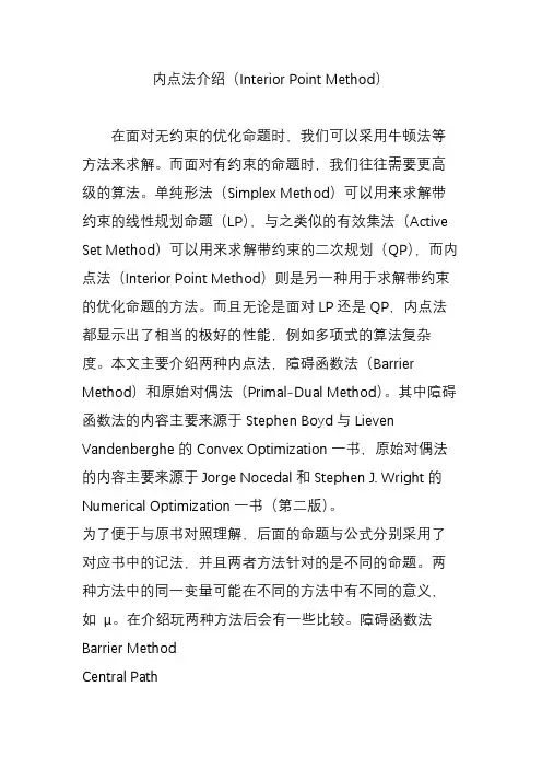
内点法介绍（Interior Point Method）在面对无约束的优化命题时，我们可以采用牛顿法等方法来求解。

而面对有约束的命题时，我们往往需要更高级的算法。

单纯形法（Simplex Method）可以用来求解带约束的线性规划命题（LP），与之类似的有效集法（Active Set Method）可以用来求解带约束的二次规划（QP），而内点法（Interior Point Method）则是另一种用于求解带约束的优化命题的方法。

而且无论是面对LP还是QP，内点法都显示出了相当的极好的性能，例如多项式的算法复杂度。

本文主要介绍两种内点法，障碍函数法（Barrier Method）和原始对偶法（Primal-Dual Method）。

其中障碍函数法的内容主要来源于Stephen Boyd与Lieven Vandenberghe的Convex Optimization一书，原始对偶法的内容主要来源于Jorge Nocedal和Stephen J. Wright的Numerical Optimization一书（第二版）。

为了便于与原书对照理解，后面的命题与公式分别采用了对应书中的记法，并且两者方法针对的是不同的命题。

两种方法中的同一变量可能在不同的方法中有不同的意义，如μ。

在介绍玩两种方法后会有一些比较。

障碍函数法Barrier MethodCentral Path举例原始对偶内点法Primal Dual Interior Point Method Central Path举例几个问题障碍函数法（Barrier Method）对于障碍函数法，我们考虑一个一般性的优化命题：minsubject tof0(x)fi(x)≤0,i=1,...,mAx=b(1) 这里f0,...,fm:Rn→R 是二阶可导的凸函数。

同时我也要求命题是有解的，即最优解x 存在，且其对应的目标函数为p。

此外，我们还假设原命题是可行的（feasible）。

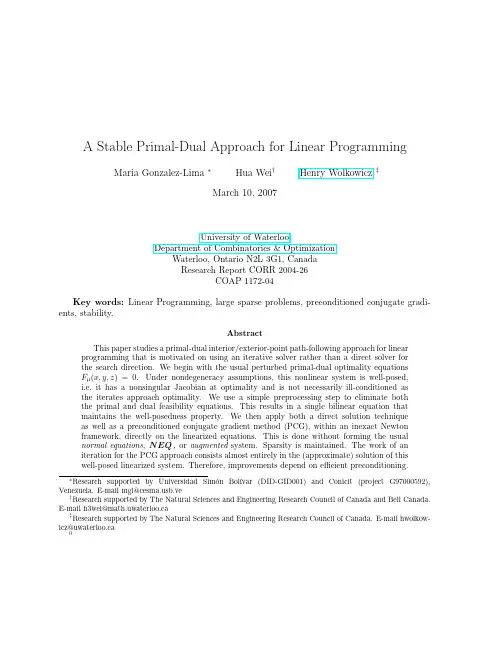
A Stable Primal-Dual Approach for Linear ProgrammingMaria Gonzalez-Lima∗Hua Wei†Henry Wolkowicz‡March10,2007University of WaterlooDepartment of Combinatorics&OptimizationWaterloo,Ontario N2L3G1,CanadaResearch Report CORR2004-26COAP1172-04Key words:Linear Programming,large sparse problems,preconditioned conjugate gradi-ents,stability.AbstractThis paper studies a primal-dual interior/exterior-point path-following approach for linear programming that is motivated on using an iterative solver rather than a direct solver forthe search direction.We begin with the usual perturbed primal-dual optimality equationsFµ(x,y,z)=0.Under nondegeneracy assumptions,this nonlinear system is well-posed,i.e.it has a nonsingular Jacobian at optimality and is not necessarily ill-conditioned asthe iterates approach optimality.We use a simple preprocessing step to eliminate boththe primal and dual feasibility equations.This results in a single bilinear equation thatmaintains the well-posedness property.We then apply both a direct solution techniqueas well as a preconditioned conjugate gradient method(PCG),within an inexact Newtonframework,directly on the linearized equations.This is done without forming the usualnormal equations,NEQ,or augmented system.Sparsity is maintained.The work of aniteration for the PCG approach consists almost entirely in the(approximate)solution of thiswell-posed linearized system.Therefore,improvements depend on efficient preconditioning.。

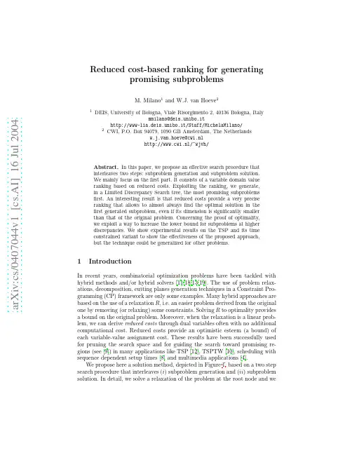
a rXi v :c s /04744v1[cs.A I]16J ul24Reduced cost-based ranking for generating promising subproblems ano 1and W.J.van Hoeve 21DEIS,University of Bologna,Viale Risorgimento 2,40136Bologna,Italy mmilano@deis.unibo.it http://www-lia.deis.unibo.it/Staff/MichelaMilano/2CWI,P.O.Box 94079,1090GB Amsterdam,The Netherlands w.j.van.hoeve@cwi.nl http://www.cwi.nl/~wjvh/Abstract.In this paper,we propose an effective search procedure that interleaves two steps:subproblem generation and subproblem solution.We mainly focus on the first part.It consists of a variable domain value ranking based on reduced costs.Exploiting the ranking,we generate,in a Limited Discrepancy Search tree,the most promising subproblems first.An interesting result is that reduced costs provide a very precise ranking that allows to almost always find the optimal solution in the first generated subproblem,even if its dimension is significantly smaller than that of the original problem.Concerning the proof of optimality,we exploit a way to increase the lower bound for subproblems at higher discrepancies.We show experimental results on the TSP and its time constrained variant to show the effectiveness of the proposed approach,but the technique could be generalized for other problems.1Introduction In recent years,combinatorial optimization problems have been tackled with hybrid methods and/or hybrid solvers [11,18,13,19].The use of problem relax-ations,decomposition,cutting planes generation techniques in a Constraint Pro-gramming (CP)framework are only some examples.Many hybrid approaches are based on the use of a relaxation R ,i.e.an easier problem derived from the originalone by removing (or relaxing)some constraints.Solving R to optimality provides a bound on the original problem.Moreover,when the relaxation is a linear prob-lem,we can derive reduced costs through dual variables often with no additional computational cost.Reduced costs provide an optimistic esteem (a bound)of each variable-value assignment cost.These results have been successfully used for pruning the search space and for guiding the search toward promising re-gions (see [9])in many applications like TSP [12],TSPTW [10],scheduling with sequence dependent setup times [8]and multimedia applications [4].We propose here a solution method,depicted in Figure 1,based on a two step search procedure that interleaves (i )subproblem generation and (ii )subproblem solution.In detail,we solve a relaxation of the problem at the root node and we2use reduced costs to rank domain values;then we partition the domain of eachvariable X i in two sets,i.e.,the good part D goodi and the bad part D badi.We searchthe tree generated by using a strategy imposing on the left branch the branchingconstraint X i∈D goodi while on the right branch we impose X i∈D badi.At eachleaf of the subproblem generation tree,we have a subproblem which can now be solved(in the subproblem solution tree).Exploring with a Limited Discrepancy Strategy the resulting search space, we obtain that thefirst generated subproblems are supposed to be the most promising and are likely to contain the optimal solution.In fact,if the ranking criterion is effective(as the experimental results will show),thefirst generated subproblem(discrepancy equal to0)P(0),where all variables range on the good domain part,is likely to contain the optimal solution.The following generatedsubproblems(discrepancy equal to1)P(1)i have all variables but the i-th rangingon the good domain and are likely to contain worse solutions with respect to P(0),but still good.Clearly,subproblems at higher discrepancies are supposed to contain the worst solutions.A surprising aspect of this method is that even by using low cardinality good sets,we almost alwaysfind the optimal solution in thefirst gener-ated subproblem.Thus,reduced costs provide extremely useful information indicating for each variable which values are the most promising.Moreover,this property of reduced costs is independent of the tightness of the relaxation.Tight relaxations are essential for the proof of optimality,but not for the quality of reduced costs.Solving only thefirst subproblem,we obtain a very effective in-complete method thatfinds the optimal solution in almost all test instances.To be complete,the method should solve all subproblems for all discrepancies to prove optimality.Clearly,even if each subproblem could be efficiently solved,if all of them should be considered,the proposed approach would not be applicable. The idea is that by generating the optimal solution soon and tightening the lower bound with considerations based on the discrepancies shown in the paper,we do not have to explore all subproblems,but we can prune many of them.In this paper,we have considered as an example the Travelling Salesman Problem and its time constrained variant,but the technique could be applied to a large family of problems.The contribution of this paper is twofold:(i)we show that reduced costs provide an extremely precise indication for generating promising subproblems, and(ii)we show that LDS can be used to effectively order the subproblems. In addition,the use of discrepancies enables to tighten the problem bounds for each subproblem.The paper is organized as follows:in Section2we give preliminaries on Lim-ited Discrepancy Search(LDS),on the TSP and its time constrained variant. In Section3we describe the proposed method in detail.Section4discusses the implementation,focussing mainly on the generation of the subproblems using LDS.The quality of the reduced cost-based ranking is considered in Section5. In this section also the size of subproblems is tuned.Section6presents the computational results.Conclusion and future work follow.3Fig.1.The structure of the search tree.2Preliminaries2.1Limited Discrepancy SearchLimited Discrepancy Search(LDS)wasfirst introduced by Harvey and Ginsberg[15].The idea is that one can oftenfind the optimal solution by exploring onlya small fraction of the space by relying on tuned(often problem dependent) heuristics.However,a perfect heuristic is not always available.LDS addresses the problem of what to do when the heuristic fails.Thus,at each node of the search tree,the heuristic is supposed to provide the good choice(corresponding to the leftmost branch)among possible alternative branches.Any other choice would be bad and is called a discrepancy.In LDS, one tries tofindfirst the solution with as few discrepancies as possible.In fact,a perfect heuristic would provide us the optimal solution immediately.Since this is not often the case,we have to increase the number of discrepancies so as to make it possible tofind the optimal solution after correcting the mistakes made by the heuristic.However,the goal is to use only few discrepancies since in general good solutions are provided soon.LDS builds a search tree in the following way:thefirst solution explored is that suggested by the heuristic.Then solutions that follow the heuristic for every variable but one are explored:these solutions are that of discrepancy equal to one.Then,solutions at discrepancy equal to two are explored and so on.It has been shown that this search strategy achieves a significant cutoffof the total number of nodes with respect to a depthfirst search with chronological backtracking and iterative sampling[20].42.2TSP and TSPTWLet G=(V,A)be a digraph,where V={1,...,n}is the vertex set and A= {(i,j):i,j∈V}the arc set,and let c ij≥0be the cost associated with arc (i,j)∈A(with c ii=+∞for each i∈V).A Hamiltonian Circuit(tour)of G is a partial digraph¯G=(V,¯A)of G such that:|¯A|=n and for each pair of distinct vertices v1,v2∈V,both paths from v1to v2and from v2to v1exist in¯G(i.e. digraph¯G is strongly connected).The Travelling Salesman Problem(TSP)looks for a Hamiltonian circuit G∗= (V,A∗)whose cost (i,j)∈A∗c ij is a minimum.A classic Integer Linear Programming formulation for TSP is as follows:v(T SP)=min i∈V j∈V c ij x ij(1)subject to i∈V x ij=1,j∈V(2)j∈V x ij=1,i∈V(3)i∈Sj∈V\Sx ij≥1,S⊂V,S=∅(4)x ij integer,i,j∈V(5) where x ij=1if and only if arc(i,j)is part of the solution.Constraints(2) and(3)impose in-degree and out-degree of each vertex equal to one,whereas constraints(4)impose strong connectivity.Constraint Programming relies in general on a different model where we have a domain variable Next i(resp.Prev i)that identifies cities visited after(resp. before)node i.Domain variable Cost i identifies the cost to be paid to go from node i to node Next i.Clearly,we need a mapping between the CP model and the ILP model: Next i=j⇔x ij=1.The domain of variable Next i will be denoted as D i. Initially,D i={1,...,n}.The Travelling Salesman Problem with Time Windows(TSPTW)is a time constrained variant of the TSP where the service at a node i should begin within a time window[a i,b i]associated to the node.Early arrivals are allowed,in the sense that the vehicle can arrive before the time window lower bound.However, in this case the vehicle has to wait until the node is ready for the beginning of service.As concerns the CP model for the TSPTW,we add to the TSP model a domain variable Start i which identifies the time at which the service begins at node i.A well known relaxation of the TSP and TSPTW obtained by eliminating from the TSP model constraints(4)and time windows constraints is the Linear Assignment Problem(AP)(see[3]for a survey).AP is the graph theory problem5 offinding a set of disjoint subtours such that all the vertices in V are visited and the overall cost is a minimum.When the digraph is complete,as in our case,AP always has an optimal integer solution,and,if such solution is composed by a single tour,is then optimal for TSP satisfying constraints(4).The information provided by the AP relaxation is a lower bound LB for the original problem and the reduced cost matrix¯c.At each node of the decision tree,each¯c ij estimates the additional cost to pay to put arc(i,j)in the so-lution.More formally,a valid lower bound for the problem where x ij=1isLB|xij =1=LB+¯c ij.It is well-known that when the AP optimal solution isobtained through a primal-dual algorithm,as in our case(we use a C++adap-tation of the AP code described in[2]),the reduced cost values are obtained without extra computational effort during the AP solution.The solution of the AP relaxation at the root node requires in the worst case O(n3),whereas each following AP solution can be efficiently computed in O(n2)time through a single augmenting path step(see[2]for details).However,the AP does not provide a tight bound neither for the TSP nor for the TSPTW.Therefore we will improve the relaxation in Section3.1.3The Proposed MethodIn this section we describe the method proposed in this paper.It is based on two interleaved steps:subproblem generation and subproblem solution.Thefirst step is based on the optimal solution of a(possibly tight)relaxation of the original problem.The relaxation provides a lower bound for the original problem and the reduced cost matrix.Reduced costs are used for ranking(the lower the better)variable domain values.Each domain is now partitioned according to this ranking in two sets called the good set and the bad set.The cardinality of the good set is problem dependent and is experimentally defined.However,it should be significantly lower than the dimension of the original domains.Exploiting this ranking,the search proceeds by choosing at each node the branching constraint that imposes the variable to range on the good domain, while on backtracking we impose the variable to range on the bad domain.By exploring the resulting search tree by using an LDS strategy we generatefirst the most promising problems,i.e.,those where no or few variables range on the bad sets.Each time we generate a subproblem,the second step starts for optimally solving it.Experimental results will show that,surprisingly,even if the sub-problems are small,thefirst generated subproblem almost always contains the optimal solution.The proof of optimality should then proceed by solving the re-maining problems.Therefore,a tight initial lower bound is essential.Moreover, by using some considerations on discrepancies,we can increase the bound and prove optimality fast.The idea of ranking domain values has been previously used in incomplete algorithms,like GRASP[5].The idea is to produce for each variable the so called Restricted Candidate List(RCL),and explore the subproblem generated only by6RCLs for each variable.This method provides in general a good starting point for performing local search.Our ranking method could in principle be applied to GRASP-like algorithms.Another connection can be made with iterative broadening[14],where one can view the breadth cutoffas corresponding to the cardinality of our good sets. Thefirst generated subproblem of both approaches is then the same.However, iterative broadening behaves differently on backtracking(it gradually restarts increasing the breadth cutoff).3.1Linear relaxationIn Section2.2we presented a relaxation,the Linear Assignment Problem(AP), for both the TSP and TSPTW.This relaxation is indeed not very tight and does not provide a good lower bound.We can improve it by adding cutting planes. Many different kinds of cutting planes for these problems have been proposed and the corresponding separation procedure has been defined[22].In this paper, we used the Sub-tour Elimination Cuts(SECs)for the TSP.However,adding linear inequalities to the AP formulation changes the structure of the relaxation which is no longer an AP.On the other hand,we are interested in maintaining this structure since we have a polynomial and incremental algorithm that solves the problem.Therefore,as done in[10],we relax cuts in a Lagrangean way,thus maintaining an AP structure.The resulting relaxation,we call it AP cuts,still has an AP structure,but provides a tighter bound than the initial AP.More precisely,it provides the same objective function value as the linear relaxation where all cuts are added defining the sub-tour polytope.In many cases,in particular for TSPTW instances,the bound is extremely close to the optimal solution.3.2Domain partitioningAs described in Section2.2,the solution of an Assignment Problem provides the reduced cost matrix with no additional computational cost.We recall that the reduced costc ij.Consequently,D badi =D i\D goodi.The ratio defines the size of the good domains,and will be discussed in Section5.Note that the optimal ratio should be experimentally tuned,in order to obtain the optimal solution in thefirst subproblem,and it is strongly problem7 dependent.In particular,it depends on the structure of the problem we are solving.For instance,for the pure TSP instances considered in this paper,a good ratio is0.05or0.075,while for TSPTW the best ratio observed is around 0.15.With this ratio,the optimal solution of the original problem is indeed located in thefirst generated subproblem in almost all test instances.3.3LDS for generating subproblemsIn the previous section,we described how to partition variable domains in a good and a bad set by exploiting information on reduced costs.Now,we show how to explore a search tree on the basis of this domain partitioning.At each node corresponding to the choice of variable X i,whose domain has been parti-tioned in D goodi and D badi,we impose on the left branch the branching constraintX i∈D goodi ,and on the right branch X i∈D badi.Exploring with a Limited Dis-crepancy Search strategy this tree,wefirst explore the subproblem suggested by the heuristic where all variable range on the good set;then subproblems where all variables but one range on the good set,and so on.If the reduced cost-based ranking criterion is accurate,as the experimental results confirm,we are likely tofind the optimal solution in the subproblem P(0) generated by imposing all variables ranging on the good set of values.If this heuristic fails once,we are likely tofind the optimal solution in one of the nsubproblems(P(1)i with i∈{1,...,n})generated by imposing all variables butone(variable i)ranging on the good sets and one ranging on the bad set.Then,we go on generating n(n−1)/2problems P(2)ij all variables but two(namely iand j)ranging on the good set and two ranging on the bad set are considered, and so on.In Section4we will see an implementation of this search strategy that in a sense squeezes the subproblem generation tree shown in Figure1into a con-straint.3.4Proof of optimalityIf we are simply interested in a good solution,without proving optimality,we can stop our method after the solution of thefirst generated subproblem.In this case,the proposed approach is extremely effective since we almost alwaysfind the optimal solution in that subproblem.Otherwise,if we are interested in a provably optimal solution,we have to prove optimality by solving all sub-problems at increasing discrepancies.Clearly, even if all subproblems could be efficiently solved,generating and solving all of them would not be practical.However,if we exploit a tight initial lower bound, as explained in Section3.1,which is successively improved with considerations on the discrepancy,we can stop the generation of subproblems after few trials since we prove optimality fast.An important part of the proof of optimality is the management of lower and upper bounds.The upper bound is decreased as wefind better solutions,and8the lower bound is increased as a consequence of discrepancy increase.The idea is tofind an optimal solution in thefirst subproblem,providing the best possible upper bound.The ideal case is that all subproblems but thefirst can be pruned since they have a lower bound higher than the current upper bound,in which case we only need to consider a single subproblem.The initial lower bound LB0provided by the Assignment Problem AP cuts at the root node can be improved each time we switch to a higher discrepancy k. For i∈{1,...,n},letc∗i=min j∈D badic∗i for all problems at discrepancy greater than or equal to1.We can increase this bound:let L be the nondecreasing ordered list ofc.Now we define a second relaxation of P having cost matrix9 The search for such a set S and the corresponding domain assignments have been‘squeezed’into a constraint,the discrepancy constraint discrgood is the array containing D goodi for all i∈{1,...,n}.The command solvesubproblem is shorthand for solving the subproblem which has been considered in Section3.5.A more traditional implementation of LDS(referred to as‘standard’in Ta-ble1)exploits tree search,where at each node the domain of a variable is split into the good set or the bad set,as described in Section3.3.In Table1,the performance of this traditional approach is compared with the performance of the discrepancy constraint(referred to as discr10standard discr instance time fails0.08440.15570.05140.10690.09420.06300.12710.201520.0660.075csttime failsrbg021.20.1366 rbg021.30.20158 rbg021.40.0940 rbg021.50.16125 rbg021.60.2110 rbg021.70.2270 rbg021.80.1588 rbg021.90.17108 rbg0210.19158 rbg027a0.2153parison of traditional LDS and the discrepancy constraint. goodfirst solution and proving optimality.This is done by tuning the ratio r, which determines the size of thefirst subproblem.We recall from Section3.2that|D goodi |≤rn for i∈{1,...,n}.In Tables2and3we report the quality of the heuristic with respect to the ra-tio.The TSP instances are taken from TSPLIB[23]and the asymmetric TSPTW instances are due to Ascheuer[1].All subproblems are solved to optimality with afixed strategy,as to make a fair comparison.In the tables,‘size’is the actual relative size of thefirst subproblem with respect to the initial problem.The size is calculated by1instance size opt pr fails size opt pr fails0.250120.320170.170110.230160.170120.210120.160110.24013270.14121270.21011k0.131619k0.200165average0.200 1.17680.250175 Table2.Quality of heuristic with respect to ratio for the TSP.The domains in the TSPTW instances are typically much smaller than the number of variables,because of the time window constraints that already remove a number of domain values.Therefore,thefirst subproblem might sometimes be relatively large,since only a few values are left after pruning,and they might be equally promising.The next columns in the tables are‘opt’and‘pr’.Here‘opt’denotes the level of discrepancy at which the optimal solution is found.Typically,we would11 like this to be0.The column‘pr’stands for the level of discrepancy at which optimality is proved.This would preferably be1.The column‘fails’denotes the total number of backtracks during search needed to solve the problem to optimality.Concerning the TSP instances,already for a ratio of0.05all solutions are in thefirst subproblem.For a ratio of0.075,we can also prove optimality at discrepancy1.Taking into account also the number of fails,we can argue that both0.05and0.075are good ratio candidates for the TSP instances.For the TSPTW instances,we notice that a smaller ratio does not necessarily increase the total number of fails,although it is more difficult to prove optimality. Hence,we have a slight preference for the ratio to be0.15,mainly because of its overall(average)performance.An important aspect we are currently investigating is the dynamic tuning of the ratio.6Computational ResultsWe have implemented and tested the proposed method using ILOG Solver and Scheduler[17,16].The algorithm runs on a Pentium1Ghz,256MB RAM,and uses CPLEX6.5as LP solver.The two sets of test instances are taken from the TSPLIB[23]and Ascheuer’s asymmetric TSPTW problem instances[1].Table4shows the results for small TSP instances.Time is measured in seconds,fails again denote the total number of backtracks to prove optimality. The time limit is set to300seconds.Observe that our method(LDS)needs less number of fails than the approach without subproblem generation(No LDS). This comes with a cost,but still our approach is never slower and in some cases considerably faster.The problems were solved both with a ratio of0.05and0.075, the best of which is reported in the table.Observe that in some cases a ratio of 0.05is best,while in other cases0.075is better.For three instances optimality could not be proven directly after solving thefirst subproblem.Nevertheless the optimum was found in this subproblem(indicated by objective‘obj’is‘opt’). Time and the number of backtracks(fails)needed in thefirst subproblem are reported for these instances.In Table5the results for the asymmetric TSPTW instances are shown.Our method(LDS)uses a ratio of0.15to solve all these problems to optimality.It is compared to our code without the subproblem generation(No LDS),and to the results by Focacci,Lodi and Milano(FLM2002)[10].Up to now,FLM2002 has the fastest solution times for this set of instances,to our knowledge.When comparing the time results(measured in seconds),one should take into account that FLM2002uses a Pentium III700MHz.Our method behaves in general quite well.In many cases it is much faster than FLM2002.However,in some cases the subproblem generation does not pay off.This is for instance the case for rbg040a and rbg042a.Although our method finds the optimal solution in thefirst branch(discrepancy0)quite fast,the initial bound LB0is too low to be able to prune the search tree at discrepancy1.In those12ratio=0.05ratio=0.1ratio=0.15ratio=0.2 size opt pr fails size opt pr failsrbg010a0.940150.99017 rbg016a0.8802410.980147 rbg016b0.7203540.910239 rbg017.20.490190.660127 rbg0170.6615700.890249 rbg017a0.7201130.8801122 rbg019a0.98012710130 rbg019b0.7813850.950171 rbg019c0.60131370.760299 rbg019d0.970161016 rbg020a0.840130.94015 rbg021.20.5901480.7401148 rbg021.30.55141850.6803163 rbg021.40.5303330.670287 rbg021.50.55021030.6702206 rbg021.60.48122330.6701124 rbg021.70.4902910.650170 rbg021.80.48125180.630188 rbg021.90.48125740.6301108 rbg0210.60131370.760299 rbg027a0.5902350.7701960.570.673.0517250.740.101.5769instance size opt pr failsrbg010a10181014910149rbg016b0.9901380.7401310.900120rbg0170.9901560.9301143101236rbg019a101300.97017210172rbg019c0.920111210161016rbg020a10150.80011850.9501240rbg021.30.90021420.74021140.940170rbg021.50.88011720.73011320.9501148rbg021.70.8201780.7101890.900195rbg021.90.83011210.82021060.9501119rbg027a0.9001407average0.930 1.0510113 instance time fails ratiogr170.1210.050.0719---gr240.1810.050.1770---bayg290.28280.050.30418opt0.1936dantzig42 1.213660.07512.6115k---gr48∗19.1022k0.075limit limit opt80.3155k∗Optimality not proven directly after solvingfirst subproblem.putational results for the TSP.instance time failsrbg010a0.0660.1210.048 rbg016b0.11270.0170.042 rbg0170.0690.1220.051 rbg019a0.05110.2800.0922 rbg019c0.08170.0320.074 rbg020a0.07110.2440.0815 rbg021.30.11520.31210.0932 rbg021.50.14890.73180.1650instance time failsrbg021.70.19450.62220.1027 rbg021.90.10310.3810.1474 rbg027a0.19452.78410.68119 rbg033a0.627055.213k0.9336 rbg035a.2 5.23 2.6k3.58410.8356 rbg038a0.3742738.1136k1k387k rbg042a29.3611k180.419k 4.21 1.5k rbg055a 4.391634.049325.69128putational results for the asymmetric TSPTW.instance time fails179179014214201481480190202 6.318218201791790opt obj gap(%)rbg021.50.1019 rbg021.60.1549 rbg0210.1044 rbg035a.2 4.75 2.2k rgb040a65.8325k rbg042a33.2611.6kTable putational results for thefirst subproblem of the asymmetric TSPTW14cases we need more time to prove optimality than we would have needed if we did not apply our method(No LDS).In such cases our method can be applied as an effective incomplete method,by only solvingfirst subproblem.Table6shows the results for those instances for which optimality could not be proven directly after solving thefirst subproblem.In almost all cases the optimum is found in thefirst subproblem.7Discussion and ConclusionWe have introduced an effective search procedure that consists of generating promising subproblems and solving them.To generate the subproblems,we split the variable domains in a good part and a bad part on the basis of reduced costs. The domain values corresponding to the lowest reduced costs are more likely to be in the optimal solution,and are put into the good set.The subproblems are generated using a LDS strategy,where the discrepancy is the number of variables ranging on their bad set.Subproblems are considerably smaller than the original problem,and can be solved faster.To prove optimality, we introduced a way of increasing the lower bound using information from the discrepancies.Computational results on TSP and asymmetric TSPTW instances show that the proposed ranking is extremely accurate.In almost all cases the optimal solution is found in thefirst subproblem.When proving optimality is difficult, our method can still be used as an effective incomplete search procedure,by only solving thefirst subproblem.Some interesting points arise from the paper:first,we have seen that reduced costs represent a good ranking criterion for variable domain values.The ranking quality is not affected if reduced costs come from a loose relaxation.Second,the tightness of the lower bound is instead very important for the proof of optimality.Therefore,we have used a tight bound at the root node and increased it thus obtaining a discrepancy-based bound.Third,if we are not interested in a complete algorithm,but we need very good solutions fast,our method turns out to be a very effective choice,since the first generated subproblem almost always contains the optimal solution.Future directions will explore a different way of generating subproblems.Our domain partitioning is statically defined only at the root node and maintained during the search.However,although being static,the method is still very effec-tive.We will explore a dynamic subproblem generation. AcknowledgementsWe would like to thank Filippo Focacci and Andrea Lodi for useful discussion, suggestions and ideas.。

集合覆盖问题的模型与算法王继强【摘要】The set cover problem has favourable applications in areas of network design, but it is NP-hard in computational com-plexity. A 0-1 program model is formulated for the set cover problem. An approximation algorithm deriving from greedy idea is put forward, and is proved from the angle of primal-dual program. A case study of sensor network optimal design based on LINGO software demonstrates correctness of the model and effectiveness of the algorithm.% 集合覆盖问题在网络设计领域中有着良好的应用背景，但它在算法复杂性上却是NP-困难问题。

建立了集合覆盖问题的0-1规划模型，给出了源于贪心思想的近似算法，并从原始-对偶规划的角度进行了证明，基于LINGO软件的传感器网络最优设计案例验证了模型的正确性和算法的有效性。

【期刊名称】《计算机工程与应用》【年(卷),期】2013(000)017【总页数】4页(P15-17,72)【关键词】集合覆盖;近似算法;0-1规划;对偶规划;线性交互式通用优化器(LINGO)【作者】王继强【作者单位】山东财经大学数学与数量经济学院，济南 250014【正文语种】中文【中图分类】Q784;TP301.61 引言集合覆盖问题是组合最优化和理论计算机科学中的一类典型问题，它要求以最小代价将某一集合利用其若干子集加以覆盖。