Akhtar_Bayesian_Sparse_Representation_2015_CVPR_paper

专利名称：用于生成病人特有的、解剖学结构的基于数字图像的模型的系统和方法
专利类型：发明专利
发明人：艾纳夫·纳梅尔·叶林,兰·布龙施泰因,波阿斯·道夫·塔尔
申请号：CN201280015703.0
申请日：20120125
公开号：CN103460214A
公开日：
20131218
专利内容由知识产权出版社提供
摘要：本发明的实施方式针对执行图像引导手术的计算机仿真的方法。

所述方法可以包含接收特定病人的医学图像数据和元数据。

基于所述医学图像数据和所述元数据可以生成病人特有的、解剖学结构的基于数字图像的模型。

利用所述基于数字图像的模型和所述元数据可以执行图像引导手术的计算机仿真。

申请人：西姆博尼克斯有限公司
地址：以色列空港城
国籍：IL
代理机构：北京安信方达知识产权代理有限公司
更多信息请下载全文后查看。

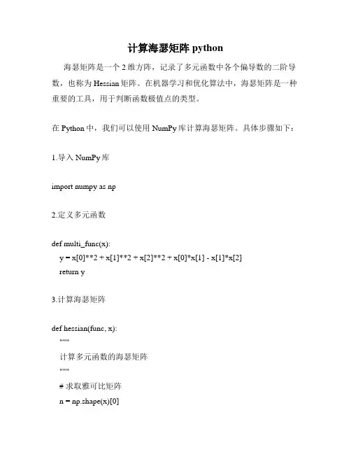
计算海瑟矩阵python海瑟矩阵是一个2维方阵，记录了多元函数中各个偏导数的二阶导数，也称为Hessian矩阵。

在机器学习和优化算法中，海瑟矩阵是一种重要的工具，用于判断函数极值点的类型。

在Python中，我们可以使用NumPy库计算海瑟矩阵。

具体步骤如下：1.导入NumPy库import numpy as np2.定义多元函数def multi_func(x):y = x[0]**2 + x[1]**2 + x[2]**2 + x[0]*x[1] - x[1]*x[2]return y3.计算海瑟矩阵def hessian(func, x):"""计算多元函数的海瑟矩阵"""# 求取雅可比矩阵n = np.shape(x)[0]jac = np.zeros((n, n))eps = np.finfo(float).epsfor i in range(n):x1 = x.copy()x2 = x.copy()x1[i] += epsx2[i] -= epsjac[:, i] = (func(x1) - func(x2)) / (2*eps)# 求取海瑟矩阵hess = np.zeros((n, n))for i in range(n):x1 = x.copy()x1[i] += epshess[i, i] = (func(x1) - 2*func(x) + func(x1)) / eps ** 2 for j in range(i+1, n):x1[i] += epsx1[j] += epshess[i, j] = (func(x1) - func(x) - jac[j, i]*eps) / eps ** 2 hess[j, i] = hess[i, j]return hessx = np.array([1, 2, 3])hess = hessian(multi_func, x)print(hess)4.结果输出输出结果为：[[ 2. 1. 0.][ 1. 2. -1.][ 0. -1. 2.]]说明该多元函数在点(x1,x2,x3) = (1,2,3)处的海瑟矩阵为[[2,1,0],[1,2,-1],[0,-1,2]]。

机器学习专业词汇中英⽂对照activation 激活值activation function 激活函数additive noise 加性噪声autoencoder ⾃编码器Autoencoders ⾃编码算法average firing rate 平均激活率average sum-of-squares error 均⽅差backpropagation 后向传播basis 基basis feature vectors 特征基向量batch gradient ascent 批量梯度上升法Bayesian regularization method 贝叶斯规则化⽅法Bernoulli random variable 伯努利随机变量bias term 偏置项binary classfication ⼆元分类class labels 类型标记concatenation 级联conjugate gradient 共轭梯度contiguous groups 联通区域convex optimization software 凸优化软件convolution 卷积cost function 代价函数covariance matrix 协⽅差矩阵DC component 直流分量decorrelation 去相关degeneracy 退化demensionality reduction 降维derivative 导函数diagonal 对⾓线diffusion of gradients 梯度的弥散eigenvalue 特征值eigenvector 特征向量error term 残差feature matrix 特征矩阵feature standardization 特征标准化feedforward architectures 前馈结构算法feedforward neural network 前馈神经⽹络feedforward pass 前馈传导fine-tuned 微调first-order feature ⼀阶特征forward pass 前向传导forward propagation 前向传播Gaussian prior ⾼斯先验概率generative model ⽣成模型gradient descent 梯度下降Greedy layer-wise training 逐层贪婪训练⽅法grouping matrix 分组矩阵Hadamard product 阿达马乘积Hessian matrix Hessian 矩阵hidden layer 隐含层hidden units 隐藏神经元Hierarchical grouping 层次型分组higher-order features 更⾼阶特征highly non-convex optimization problem ⾼度⾮凸的优化问题histogram 直⽅图hyperbolic tangent 双曲正切函数hypothesis 估值，假设identity activation function 恒等激励函数IID 独⽴同分布illumination 照明inactive 抑制independent component analysis 独⽴成份分析input domains 输⼊域input layer 输⼊层intensity 亮度/灰度intercept term 截距KL divergence 相对熵KL divergence KL分散度k-Means K-均值learning rate 学习速率least squares 最⼩⼆乘法linear correspondence 线性响应linear superposition 线性叠加line-search algorithm 线搜索算法local mean subtraction 局部均值消减local optima 局部最优解logistic regression 逻辑回归loss function 损失函数low-pass filtering 低通滤波magnitude 幅值MAP 极⼤后验估计maximum likelihood estimation 极⼤似然估计mean 平均值MFCC Mel 倒频系数multi-class classification 多元分类neural networks 神经⽹络neuron 神经元Newton’s method ⽜顿法non-convex function ⾮凸函数non-linear feature ⾮线性特征norm 范式norm bounded 有界范数norm constrained 范数约束normalization 归⼀化numerical roundoff errors 数值舍⼊误差numerically checking 数值检验numerically reliable 数值计算上稳定object detection 物体检测objective function ⽬标函数off-by-one error 缺位错误orthogonalization 正交化output layer 输出层overall cost function 总体代价函数over-complete basis 超完备基over-fitting 过拟合parts of objects ⽬标的部件part-whole decompostion 部分-整体分解PCA 主元分析penalty term 惩罚因⼦per-example mean subtraction 逐样本均值消减pooling 池化pretrain 预训练principal components analysis 主成份分析quadratic constraints ⼆次约束RBMs 受限Boltzman机reconstruction based models 基于重构的模型reconstruction cost 重建代价reconstruction term 重构项redundant 冗余reflection matrix 反射矩阵regularization 正则化regularization term 正则化项rescaling 缩放robust 鲁棒性run ⾏程second-order feature ⼆阶特征sigmoid activation function S型激励函数significant digits 有效数字singular value 奇异值singular vector 奇异向量smoothed L1 penalty 平滑的L1范数惩罚Smoothed topographic L1 sparsity penalty 平滑地形L1稀疏惩罚函数smoothing 平滑Softmax Regresson Softmax回归sorted in decreasing order 降序排列source features 源特征sparse autoencoder 消减归⼀化Sparsity 稀疏性sparsity parameter 稀疏性参数sparsity penalty 稀疏惩罚square function 平⽅函数squared-error ⽅差stationary 平稳性（不变性）stationary stochastic process 平稳随机过程step-size 步长值supervised learning 监督学习symmetric positive semi-definite matrix 对称半正定矩阵symmetry breaking 对称失效tanh function 双曲正切函数the average activation 平均活跃度the derivative checking method 梯度验证⽅法the empirical distribution 经验分布函数the energy function 能量函数the Lagrange dual 拉格朗⽇对偶函数the log likelihood 对数似然函数the pixel intensity value 像素灰度值the rate of convergence 收敛速度topographic cost term 拓扑代价项topographic ordered 拓扑秩序transformation 变换translation invariant 平移不变性trivial answer 平凡解under-complete basis 不完备基unrolling 组合扩展unsupervised learning ⽆监督学习variance ⽅差vecotrized implementation 向量化实现vectorization ⽮量化visual cortex 视觉⽪层weight decay 权重衰减weighted average 加权平均值whitening ⽩化zero-mean 均值为零Letter AAccumulated error backpropagation 累积误差逆传播Activation Function 激活函数Adaptive Resonance Theory/ART ⾃适应谐振理论Addictive model 加性学习Adversarial Networks 对抗⽹络Affine Layer 仿射层Affinity matrix 亲和矩阵Agent 代理 / 智能体Algorithm 算法Alpha-beta pruning α-β剪枝Anomaly detection 异常检测Approximation 近似Area Under ROC Curve／AUC Roc 曲线下⾯积Artificial General Intelligence/AGI 通⽤⼈⼯智能Artificial Intelligence/AI ⼈⼯智能Association analysis 关联分析Attention mechanism 注意⼒机制Attribute conditional independence assumption 属性条件独⽴性假设Attribute space 属性空间Attribute value 属性值Autoencoder ⾃编码器Automatic speech recognition ⾃动语⾳识别Automatic summarization ⾃动摘要Average gradient 平均梯度Average-Pooling 平均池化Letter BBackpropagation Through Time 通过时间的反向传播Backpropagation/BP 反向传播Base learner 基学习器Base learning algorithm 基学习算法Batch Normalization/BN 批量归⼀化Bayes decision rule 贝叶斯判定准则Bayes Model Averaging／BMA 贝叶斯模型平均Bayes optimal classifier 贝叶斯最优分类器Bayesian decision theory 贝叶斯决策论Bayesian network 贝叶斯⽹络Between-class scatter matrix 类间散度矩阵Bias 偏置 / 偏差Bias-variance decomposition 偏差-⽅差分解Bias-Variance Dilemma 偏差 – ⽅差困境Bi-directional Long-Short Term Memory/Bi-LSTM 双向长短期记忆Binary classification ⼆分类Binomial test ⼆项检验Bi-partition ⼆分法Boltzmann machine 玻尔兹曼机Bootstrap sampling ⾃助采样法／可重复采样／有放回采样Bootstrapping ⾃助法Break-Event Point／BEP 平衡点Letter CCalibration 校准Cascade-Correlation 级联相关Categorical attribute 离散属性Class-conditional probability 类条件概率Classification and regression tree/CART 分类与回归树Classifier 分类器Class-imbalance 类别不平衡Closed -form 闭式Cluster 簇/类/集群Cluster analysis 聚类分析Clustering 聚类Clustering ensemble 聚类集成Co-adapting 共适应Coding matrix 编码矩阵COLT 国际学习理论会议Committee-based learning 基于委员会的学习Competitive learning 竞争型学习Component learner 组件学习器Comprehensibility 可解释性Computation Cost 计算成本Computational Linguistics 计算语⾔学Computer vision 计算机视觉Concept drift 概念漂移Concept Learning System /CLS 概念学习系统Conditional entropy 条件熵Conditional mutual information 条件互信息Conditional Probability Table／CPT 条件概率表Conditional random field/CRF 条件随机场Conditional risk 条件风险Confidence 置信度Confusion matrix 混淆矩阵Connection weight 连接权Connectionism 连结主义Consistency ⼀致性／相合性Contingency table 列联表Continuous attribute 连续属性Convergence 收敛Conversational agent 会话智能体Convex quadratic programming 凸⼆次规划Convexity 凸性Convolutional neural network/CNN 卷积神经⽹络Co-occurrence 同现Correlation coefficient 相关系数Cosine similarity 余弦相似度Cost curve 成本曲线Cost Function 成本函数Cost matrix 成本矩阵Cost-sensitive 成本敏感Cross entropy 交叉熵Cross validation 交叉验证Crowdsourcing 众包Curse of dimensionality 维数灾难Cut point 截断点Cutting plane algorithm 割平⾯法Letter DData mining 数据挖掘Data set 数据集Decision Boundary 决策边界Decision stump 决策树桩Decision tree 决策树／判定树Deduction 演绎Deep Belief Network 深度信念⽹络Deep Convolutional Generative Adversarial Network/DCGAN 深度卷积⽣成对抗⽹络Deep learning 深度学习Deep neural network/DNN 深度神经⽹络Deep Q-Learning 深度 Q 学习Deep Q-Network 深度 Q ⽹络Density estimation 密度估计Density-based clustering 密度聚类Differentiable neural computer 可微分神经计算机Dimensionality reduction algorithm 降维算法Directed edge 有向边Disagreement measure 不合度量Discriminative model 判别模型Discriminator 判别器Distance measure 距离度量Distance metric learning 距离度量学习Distribution 分布Divergence 散度Diversity measure 多样性度量／差异性度量Domain adaption 领域⾃适应Downsampling 下采样D-separation （Directed separation）有向分离Dual problem 对偶问题Dummy node 哑结点Dynamic Fusion 动态融合Dynamic programming 动态规划Letter EEigenvalue decomposition 特征值分解Embedding 嵌⼊Emotional analysis 情绪分析Empirical conditional entropy 经验条件熵Empirical entropy 经验熵Empirical error 经验误差Empirical risk 经验风险End-to-End 端到端Energy-based model 基于能量的模型Ensemble learning 集成学习Ensemble pruning 集成修剪Error Correcting Output Codes／ECOC 纠错输出码Error rate 错误率Error-ambiguity decomposition 误差-分歧分解Euclidean distance 欧⽒距离Evolutionary computation 演化计算Expectation-Maximization 期望最⼤化Expected loss 期望损失Exploding Gradient Problem 梯度爆炸问题Exponential loss function 指数损失函数Extreme Learning Machine/ELM 超限学习机Letter FFactorization 因⼦分解False negative 假负类False positive 假正类False Positive Rate/FPR 假正例率Feature engineering 特征⼯程Feature selection 特征选择Feature vector 特征向量Featured Learning 特征学习Feedforward Neural Networks/FNN 前馈神经⽹络Fine-tuning 微调Flipping output 翻转法Fluctuation 震荡Forward stagewise algorithm 前向分步算法Frequentist 频率主义学派Full-rank matrix 满秩矩阵Functional neuron 功能神经元Letter GGain ratio 增益率Game theory 博弈论Gaussian kernel function ⾼斯核函数Gaussian Mixture Model ⾼斯混合模型General Problem Solving 通⽤问题求解Generalization 泛化Generalization error 泛化误差Generalization error bound 泛化误差上界Generalized Lagrange function ⼴义拉格朗⽇函数Generalized linear model ⼴义线性模型Generalized Rayleigh quotient ⼴义瑞利商Generative Adversarial Networks/GAN ⽣成对抗⽹络Generative Model ⽣成模型Generator ⽣成器Genetic Algorithm/GA 遗传算法Gibbs sampling 吉布斯采样Gini index 基尼指数Global minimum 全局最⼩Global Optimization 全局优化Gradient boosting 梯度提升Gradient Descent 梯度下降Graph theory 图论Ground-truth 真相／真实Letter HHard margin 硬间隔Hard voting 硬投票Harmonic mean 调和平均Hesse matrix 海塞矩阵Hidden dynamic model 隐动态模型Hidden layer 隐藏层Hidden Markov Model/HMM 隐马尔可夫模型Hierarchical clustering 层次聚类Hilbert space 希尔伯特空间Hinge loss function 合页损失函数Hold-out 留出法Homogeneous 同质Hybrid computing 混合计算Hyperparameter 超参数Hypothesis 假设Hypothesis test 假设验证Letter IICML 国际机器学习会议Improved iterative scaling/IIS 改进的迭代尺度法Incremental learning 增量学习Independent and identically distributed/i.i.d. 独⽴同分布Independent Component Analysis/ICA 独⽴成分分析Indicator function 指⽰函数Individual learner 个体学习器Induction 归纳Inductive bias 归纳偏好Inductive learning 归纳学习Inductive Logic Programming／ILP 归纳逻辑程序设计Information entropy 信息熵Information gain 信息增益Input layer 输⼊层Insensitive loss 不敏感损失Inter-cluster similarity 簇间相似度International Conference for Machine Learning/ICML 国际机器学习⼤会Intra-cluster similarity 簇内相似度Intrinsic value 固有值Isometric Mapping/Isomap 等度量映射Isotonic regression 等分回归Iterative Dichotomiser 迭代⼆分器Letter KKernel method 核⽅法Kernel trick 核技巧Kernelized Linear Discriminant Analysis／KLDA 核线性判别分析K-fold cross validation k 折交叉验证／k 倍交叉验证K-Means Clustering K – 均值聚类K-Nearest Neighbours Algorithm/KNN K近邻算法Knowledge base 知识库Knowledge Representation 知识表征Letter LLabel space 标记空间Lagrange duality 拉格朗⽇对偶性Lagrange multiplier 拉格朗⽇乘⼦Laplace smoothing 拉普拉斯平滑Laplacian correction 拉普拉斯修正Latent Dirichlet Allocation 隐狄利克雷分布Latent semantic analysis 潜在语义分析Latent variable 隐变量Lazy learning 懒惰学习Learner 学习器Learning by analogy 类⽐学习Learning rate 学习率Learning Vector Quantization/LVQ 学习向量量化Least squares regression tree 最⼩⼆乘回归树Leave-One-Out/LOO 留⼀法linear chain conditional random field 线性链条件随机场Linear Discriminant Analysis／LDA 线性判别分析Linear model 线性模型Linear Regression 线性回归Link function 联系函数Local Markov property 局部马尔可夫性Local minimum 局部最⼩Log likelihood 对数似然Log odds／logit 对数⼏率Logistic Regression Logistic 回归Log-likelihood 对数似然Log-linear regression 对数线性回归Long-Short Term Memory/LSTM 长短期记忆Loss function 损失函数Letter MMachine translation/MT 机器翻译Macron-P 宏查准率Macron-R 宏查全率Majority voting 绝对多数投票法Manifold assumption 流形假设Manifold learning 流形学习Margin theory 间隔理论Marginal distribution 边际分布Marginal independence 边际独⽴性Marginalization 边际化Markov Chain Monte Carlo/MCMC 马尔可夫链蒙特卡罗⽅法Markov Random Field 马尔可夫随机场Maximal clique 最⼤团Maximum Likelihood Estimation/MLE 极⼤似然估计／极⼤似然法Maximum margin 最⼤间隔Maximum weighted spanning tree 最⼤带权⽣成树Max-Pooling 最⼤池化Mean squared error 均⽅误差Meta-learner 元学习器Metric learning 度量学习Micro-P 微查准率Micro-R 微查全率Minimal Description Length/MDL 最⼩描述长度Minimax game 极⼩极⼤博弈Misclassification cost 误分类成本Mixture of experts 混合专家Momentum 动量Moral graph 道德图／端正图Multi-class classification 多分类Multi-document summarization 多⽂档摘要Multi-layer feedforward neural networks 多层前馈神经⽹络Multilayer Perceptron/MLP 多层感知器Multimodal learning 多模态学习Multiple Dimensional Scaling 多维缩放Multiple linear regression 多元线性回归Multi-response Linear Regression ／MLR 多响应线性回归Mutual information 互信息Letter NNaive bayes 朴素贝叶斯Naive Bayes Classifier 朴素贝叶斯分类器Named entity recognition 命名实体识别Nash equilibrium 纳什均衡Natural language generation/NLG ⾃然语⾔⽣成Natural language processing ⾃然语⾔处理Negative class 负类Negative correlation 负相关法Negative Log Likelihood 负对数似然Neighbourhood Component Analysis/NCA 近邻成分分析Neural Machine Translation 神经机器翻译Neural Turing Machine 神经图灵机Newton method ⽜顿法NIPS 国际神经信息处理系统会议No Free Lunch Theorem／NFL 没有免费的午餐定理Noise-contrastive estimation 噪⾳对⽐估计Nominal attribute 列名属性Non-convex optimization ⾮凸优化Nonlinear model ⾮线性模型Non-metric distance ⾮度量距离Non-negative matrix factorization ⾮负矩阵分解Non-ordinal attribute ⽆序属性Non-Saturating Game ⾮饱和博弈Norm 范数Normalization 归⼀化Nuclear norm 核范数Numerical attribute 数值属性Letter OObjective function ⽬标函数Oblique decision tree 斜决策树Occam’s razor 奥卡姆剃⼑Odds ⼏率Off-Policy 离策略One shot learning ⼀次性学习One-Dependent Estimator／ODE 独依赖估计On-Policy 在策略Ordinal attribute 有序属性Out-of-bag estimate 包外估计Output layer 输出层Output smearing 输出调制法Overfitting 过拟合／过配Oversampling 过采样Letter PPaired t-test 成对 t 检验Pairwise 成对型Pairwise Markov property 成对马尔可夫性Parameter 参数Parameter estimation 参数估计Parameter tuning 调参Parse tree 解析树Particle Swarm Optimization/PSO 粒⼦群优化算法Part-of-speech tagging 词性标注Perceptron 感知机Performance measure 性能度量Plug and Play Generative Network 即插即⽤⽣成⽹络Plurality voting 相对多数投票法Polarity detection 极性检测Polynomial kernel function 多项式核函数Pooling 池化Positive class 正类Positive definite matrix 正定矩阵Post-hoc test 后续检验Post-pruning 后剪枝potential function 势函数Precision 查准率／准确率Prepruning 预剪枝Principal component analysis/PCA 主成分分析Principle of multiple explanations 多释原则Prior 先验Probability Graphical Model 概率图模型Proximal Gradient Descent/PGD 近端梯度下降Pruning 剪枝Pseudo-label 伪标记Letter QQuantized Neural Network 量⼦化神经⽹络Quantum computer 量⼦计算机Quantum Computing 量⼦计算Quasi Newton method 拟⽜顿法Letter RRadial Basis Function／RBF 径向基函数Random Forest Algorithm 随机森林算法Random walk 随机漫步Recall 查全率／召回率Receiver Operating Characteristic/ROC 受试者⼯作特征Rectified Linear Unit/ReLU 线性修正单元Recurrent Neural Network 循环神经⽹络Recursive neural network 递归神经⽹络Reference model 参考模型Regression 回归Regularization 正则化Reinforcement learning/RL 强化学习Representation learning 表征学习Representer theorem 表⽰定理reproducing kernel Hilbert space/RKHS 再⽣核希尔伯特空间Re-sampling 重采样法Rescaling 再缩放Residual Mapping 残差映射Residual Network 残差⽹络Restricted Boltzmann Machine/RBM 受限玻尔兹曼机Restricted Isometry Property/RIP 限定等距性Re-weighting 重赋权法Robustness 稳健性/鲁棒性Root node 根结点Rule Engine 规则引擎Rule learning 规则学习Letter SSaddle point 鞍点Sample space 样本空间Sampling 采样Score function 评分函数Self-Driving ⾃动驾驶Self-Organizing Map／SOM ⾃组织映射Semi-naive Bayes classifiers 半朴素贝叶斯分类器Semi-Supervised Learning 半监督学习semi-Supervised Support Vector Machine 半监督⽀持向量机Sentiment analysis 情感分析Separating hyperplane 分离超平⾯Sigmoid function Sigmoid 函数Similarity measure 相似度度量Simulated annealing 模拟退⽕Simultaneous localization and mapping 同步定位与地图构建Singular Value Decomposition 奇异值分解Slack variables 松弛变量Smoothing 平滑Soft margin 软间隔Soft margin maximization 软间隔最⼤化Soft voting 软投票Sparse representation 稀疏表征Sparsity 稀疏性Specialization 特化Spectral Clustering 谱聚类Speech Recognition 语⾳识别Splitting variable 切分变量Squashing function 挤压函数Stability-plasticity dilemma 可塑性-稳定性困境Statistical learning 统计学习Status feature function 状态特征函Stochastic gradient descent 随机梯度下降Stratified sampling 分层采样Structural risk 结构风险Structural risk minimization/SRM 结构风险最⼩化Subspace ⼦空间Supervised learning 监督学习／有导师学习support vector expansion ⽀持向量展式Support Vector Machine/SVM ⽀持向量机Surrogat loss 替代损失Surrogate function 替代函数Symbolic learning 符号学习Symbolism 符号主义Synset 同义词集Letter TT-Distribution Stochastic Neighbour Embedding/t-SNE T – 分布随机近邻嵌⼊Tensor 张量Tensor Processing Units/TPU 张量处理单元The least square method 最⼩⼆乘法Threshold 阈值Threshold logic unit 阈值逻辑单元Threshold-moving 阈值移动Time Step 时间步骤Tokenization 标记化Training error 训练误差Training instance 训练⽰例／训练例Transductive learning 直推学习Transfer learning 迁移学习Treebank 树库Tria-by-error 试错法True negative 真负类True positive 真正类True Positive Rate/TPR 真正例率Turing Machine 图灵机Twice-learning ⼆次学习Letter UUnderfitting ⽋拟合／⽋配Undersampling ⽋采样Understandability 可理解性Unequal cost ⾮均等代价Unit-step function 单位阶跃函数Univariate decision tree 单变量决策树Unsupervised learning ⽆监督学习／⽆导师学习Unsupervised layer-wise training ⽆监督逐层训练Upsampling 上采样Letter VVanishing Gradient Problem 梯度消失问题Variational inference 变分推断VC Theory VC维理论Version space 版本空间Viterbi algorithm 维特⽐算法Von Neumann architecture 冯 · 诺伊曼架构Letter WWasserstein GAN/WGAN Wasserstein⽣成对抗⽹络Weak learner 弱学习器Weight 权重Weight sharing 权共享Weighted voting 加权投票法Within-class scatter matrix 类内散度矩阵Word embedding 词嵌⼊Word sense disambiguation 词义消歧Letter ZZero-data learning 零数据学习Zero-shot learning 零次学习Aapproximations近似值arbitrary随意的affine仿射的arbitrary任意的amino acid氨基酸amenable经得起检验的axiom公理，原则abstract提取architecture架构，体系结构；建造业absolute绝对的arsenal军⽕库assignment分配algebra线性代数asymptotically⽆症状的appropriate恰当的Bbias偏差brevity简短，简洁；短暂broader⼴泛briefly简短的batch批量Cconvergence 收敛，集中到⼀点convex凸的contours轮廓constraint约束constant常理commercial商务的complementarity补充coordinate ascent同等级上升clipping剪下物；剪报；修剪component分量；部件continuous连续的covariance协⽅差canonical正规的，正则的concave⾮凸的corresponds相符合；相当；通信corollary推论concrete具体的事物，实在的东西cross validation交叉验证correlation相互关系convention约定cluster⼀簇centroids 质⼼，形⼼converge收敛computationally计算(机)的calculus计算Dderive获得，取得dual⼆元的duality⼆元性；⼆象性；对偶性derivation求导；得到；起源denote预⽰，表⽰，是…的标志；意味着，[逻]指称divergence 散度；发散性dimension尺度，规格；维数dot⼩圆点distortion变形density概率密度函数discrete离散的discriminative有识别能⼒的diagonal对⾓dispersion分散，散开determinant决定因素disjoint不相交的Eencounter遇到ellipses椭圆equality等式extra额外的empirical经验；观察ennmerate例举，计数exceed超过，越出expectation期望efficient⽣效的endow赋予explicitly清楚的exponential family指数家族equivalently等价的Ffeasible可⾏的forary初次尝试finite有限的，限定的forgo摒弃，放弃fliter过滤frequentist最常发⽣的forward search前向式搜索formalize使定形Ggeneralized归纳的generalization概括，归纳；普遍化；判断（根据不⾜）guarantee保证；抵押品generate形成，产⽣geometric margins⼏何边界gap裂⼝generative⽣产的；有⽣产⼒的Hheuristic启发式的；启发法；启发程序hone怀恋；磨hyperplane超平⾯Linitial最初的implement执⾏intuitive凭直觉获知的incremental增加的intercept截距intuitious直觉instantiation例⼦indicator指⽰物，指⽰器interative重复的，迭代的integral积分identical相等的；完全相同的indicate表⽰，指出invariance不变性，恒定性impose把…强加于intermediate中间的interpretation解释，翻译Jjoint distribution联合概率Llieu替代logarithmic对数的，⽤对数表⽰的latent潜在的Leave-one-out cross validation留⼀法交叉验证Mmagnitude巨⼤mapping绘图，制图；映射matrix矩阵mutual相互的，共同的monotonically单调的minor较⼩的，次要的multinomial多项的multi-class classification⼆分类问题Nnasty讨厌的notation标志，注释naïve朴素的Oobtain得到oscillate摆动optimization problem最优化问题objective function⽬标函数optimal最理想的orthogonal(⽮量，矩阵等)正交的orientation⽅向ordinary普通的occasionally偶然的Ppartial derivative偏导数property性质proportional成⽐例的primal原始的，最初的permit允许pseudocode伪代码permissible可允许的polynomial多项式preliminary预备precision精度perturbation 不安，扰乱poist假定，设想positive semi-definite半正定的parentheses圆括号posterior probability后验概率plementarity补充pictorially图像的parameterize确定…的参数poisson distribution柏松分布pertinent相关的Qquadratic⼆次的quantity量，数量；分量query疑问的Rregularization使系统化；调整reoptimize重新优化restrict限制；限定；约束reminiscent回忆往事的；提醒的；使⼈联想…的（of）remark注意random variable随机变量respect考虑respectively各⾃的；分别的redundant过多的；冗余的Ssusceptible敏感的stochastic可能的；随机的symmetric对称的sophisticated复杂的spurious假的；伪造的subtract减去；减法器simultaneously同时发⽣地；同步地suffice满⾜scarce稀有的，难得的split分解，分离subset⼦集statistic统计量successive iteratious连续的迭代scale标度sort of有⼏分的squares平⽅Ttrajectory轨迹temporarily暂时的terminology专⽤名词tolerance容忍；公差thumb翻阅threshold阈，临界theorem定理tangent正弦Uunit-length vector单位向量Vvalid有效的，正确的variance⽅差variable变量；变元vocabulary词汇valued经估价的；宝贵的Wwrapper包装分类:。

专利名称：应用计算机技术管理、合成、可视化和探索大型多参数数据集的参数
专利类型：发明专利
发明人：詹姆斯·阿尔玛罗德,约瑟夫·斯皮德伦,迈克尔·大卫·斯塔德尼斯凯
申请号：CN201780069990.6
申请日：20171213
公开号：CN109937358A
公开日：
20190625
专利内容由知识产权出版社提供
摘要：公开了计算机技术，其将创新的数据处理和可视化技术应用于诸如细胞基因表达数据的大型多参数数据集，以发现诸如细胞和基因之间的关系的新关系，并在代表这些关系的数据集内创建新的关联数据结构。

例如，基因表达数据的散点图可以在细胞视图和基因视图之间迭代地旋转，以找到用户关注的细胞群和基因集合。

申请人：佛罗乔有限责任公司
地址：美国俄勒冈州
国籍：US
代理机构：北京安信方达知识产权代理有限公司
更多信息请下载全文后查看。

Bayesian astic Processes under Learning: de Finetti Revisited

Matthew O. Jackson Ehud Kalai Revised: May 6, 1998
Abstract
Rann Smorodinsky

1
weakened to an asymptotic mixing condition, and with his conclusion of a decomposition into iid component distributions weakened to components that are learnable and su cient for prediction.
R R R
0 0
1 For example, Nyarko 1996 argues that it is important for learning results in incomplete information games to be robust to equivalent reformulations of type spaces. He discusses examples which are not robust to such reformulations. In the language of this paper the reformulations are di erent representations of the process associated with the same game and strategies.
A probability distribution governing the evolution of a stochastic process has in nitely many Bayesian representations of the form R = d . Among these, a natural representation is one whose components 's are `learnable' one can approximate by conditioning on observation of the process and `su cient for prediction' 's predictions are not aided by conditioning on observation of the process. We show the existence and uniqueness of such a representation under a suitable asymptotic mixing condition on the process. This representation can be obtained by conditioning on the tail- eld of the process, and any learnable representation that is su cient for prediction is asymptotically like the tail- eld representation. This result is related to the celebrated de Finetti theorem, but with exchangeability

专利名称：用于对阿尔茨海默病的鉴别诊断的组合测试专利类型：发明专利
发明人：K.格沃特,A.纳伯斯,J.沙尔特纳
申请号：CN201780082303.4
申请日：20171121
公开号：CN110168374A
公开日：
20190823
专利内容由知识产权出版社提供
摘要：本发明提供了一种组合的免疫红外测定法，用于将阿尔茨海默病鉴别诊断和亚分类分为不同的疾病阶段。

该方法可用于确保疾病诊断和患者分层。

该测试考虑了体液中淀粉样‑β肽和Tau蛋白二级结构分布的变化的无标记检测。

这种从天然到β‑片层富集的亚型的二级结构变化在临床疾病表现之前很多年就出现。

现在，组合方法利用这种位移进行基于液体活组织检查的诊断。

申请人：波鸿鲁尔大学
地址：德国波鸿
国籍：DE
代理机构：北京市柳沈律师事务所
更多信息请下载全文后查看。

clustering of the final segments identifies them with a proper speaker label. 2.1 Break-point hypothesis generator Once we have the speech features for each frame, instead of hypothesizing a break point in every frame of the input signal, we select a reduced set of frames for which the system estimates that the likelihood of an acoustic change is high enough. This set will contain the most silent regions in the recording. This allows us to save an important number of calculations in the ACD procedure. The hypotheses of the ACD are the initial and final time points of the hypothesized segments. To decide whether a frame belongs to a silence region or not we only take into account the frame energy. It is essential to know the characteristics of the silence and the speech with respect to their energy and automatically obtain them from the new recordings to be processed. As a first step, we obtain the energy histogram and set a threshold to split it into two regions. An example is shown in Fig. 2, where we represent the energy in dB in abscissas plotted against the number of frames.

(0,2) 插值||(0,2) interpolation0#||zero-sharp; 读作零井或零开。

0+||zero-dagger; 读作零正。

1-因子||1-factor3-流形||3-manifold; 又称“三维流形”。

AIC准则||AIC criterion, Akaike information criterionAp 权||Ap-weightA稳定性||A-stability, absolute stabilityA最优设计||A-optimal designBCH 码||BCH code, Bose-Chaudhuri-Hocquenghem codeBIC准则||BIC criterion, Bayesian modification of the AICBMOA函数||analytic function of bounded mean oscillation; 全称“有界平均振动解析函数”。

BMO鞅||BMO martingaleBSD猜想||Birch and Swinnerton-Dyer conjecture; 全称“伯奇与斯温纳顿－戴尔猜想”。

B样条||B-splineC*代数||C*-algebra; 读作“C星代数”。

C0 类函数||function of class C0; 又称“连续函数类”。

CA T准则||CAT criterion, criterion for autoregressiveCM域||CM fieldCN 群||CN-groupCW 复形的同调||homology of CW complexCW复形||CW complexCW复形的同伦群||homotopy group of CW complexesCW剖分||CW decompositionCn 类函数||function of class Cn; 又称“n次连续可微函数类”。

Cp统计量||Cp-statisticC。

python 费舍尔判别法**一、费舍尔判别法简介**费舍尔判别法（Fisher Discriminant Analysis，简称FDA）是一种监督学习方法，主要用于对样本进行分类。

该方法由英国统计学家罗纳德·费舍尔（Ronald A.Fisher）于1936年提出。

费舍尔判别法基于样本的协方差矩阵和类间距离，通过寻找最优的超平面来实现对不同类别样本的划分。

**二、费舍尔判别法的原理**费舍尔判别法的核心思想是在特征空间中寻找一个超平面，使得两个类别之间的距离（类间距离）最大，同时使得每个类别内的样本点到超平面的距离（类内距离）最小。

为了实现这一目标，费舍尔判别法通过以下步骤进行：1.计算每个特征的均值向量；2.计算每个特征的类内协方差矩阵；3.计算类间的协方差矩阵；4.求解最优超平面对应的参数。

**三、Python实现费舍尔判别法的示例代码**在Python中，我们可以使用scikit-learn库实现费舍尔判别法。

以下是一个简单的示例：```pythonfrom sklearn.discriminant_analysis import FisherClassifierfrom sklearn.datasets import load_irisfrom sklearn.model_selection import train_test_split# 加载鸢尾花数据集iris = load_iris()X = iris.datay = iris.target# 划分训练集和测试集X_train, X_test, y_train, y_test = train_test_split(X, y, test_size=0.3, random_state=42)# 创建费舍尔分类器实例fisher_clf = FisherClassifier(random_state=42)# 训练模型fisher_clf.fit(X_train, y_train)# 预测y_pred = fisher_clf.predict(X_test)# 计算准确率accuracy = fisher_clf.score(X_test, y_test)print("准确率：", accuracy)```**四、费舍尔判别法的应用场景**费舍尔判别法适用于多分类问题，尤其在样本分布具有明显差异的情况下表现良好。

黑塞矩阵和模型协方差矩阵1. 黑塞矩阵的概念黑塞矩阵，又称为海森矩阵（Hessian Matrix），是二阶偏导数构成的方阵。

它在优化问题和数值计算中起到了重要的作用。

黑塞矩阵是一个对称矩阵，其中每个元素是二阶偏导数的导数矩阵。

2. 黑塞矩阵的应用黑塞矩阵在许多领域中都有广泛的应用，特别是在优化算法和机器学习中。

它可以提供有关函数局部性质的信息，例如极小值、鞍点和局部二次型特性。

黑塞矩阵的应用可以帮助优化算法更快地收敛，从而在求解问题时提高效率和准确性。

2.1 优化算法中的黑塞矩阵在优化算法中，黑塞矩阵被用来描述目标函数的曲率。

通过分析黑塞矩阵的特征值，可以判断目标函数的最小值、最大值或鞍点的存在。

根据这些信息，可以选择合适的优化算法来优化目标函数。

2.2 机器学习中的黑塞矩阵在机器学习中，黑塞矩阵有助于解决参数估计问题。

通过对参数估计模型的损失函数计算黑塞矩阵，可以得到模型参数的方差估计和相关性。

这对于模型的可靠性评估和参数的置信区间估计非常重要。

3. 模型协方差矩阵的概念模型协方差矩阵是描述模型参数之间相关性的矩阵。

它是一个对称矩阵，其中每个元素表示对应参数之间的协方差。

模型协方差矩阵可以通过训练数据和模型参数的估计得到。

3.1 协方差矩阵的定义协方差矩阵是描述两个随机变量之间关系的矩阵。

在机器学习中，模型参数可以视为随机变量，其协方差矩阵用于表示参数之间的关系。

协方差矩阵的对角线元素表示各个参数的方差，非对角线元素表示参数之间的协方差。

3.2 模型协方差矩阵的应用模型协方差矩阵在机器学习中被广泛应用于参数估计、模型选择和模型优化等方面。

它可以提供关于参数的置信区间、参数选择的准则和模型优化的方向等重要信息。

4. 黑塞矩阵和模型协方差矩阵之间的关系黑塞矩阵和模型协方差矩阵之间存在一定的联系。

在某些情况下，黑塞矩阵的逆和模型参数的方差估计矩阵相等。

4.1 黑塞矩阵和模型协方差矩阵的关系对于具有凸损失函数的模型，黑塞矩阵的逆等于模型参数的方差估计矩阵。

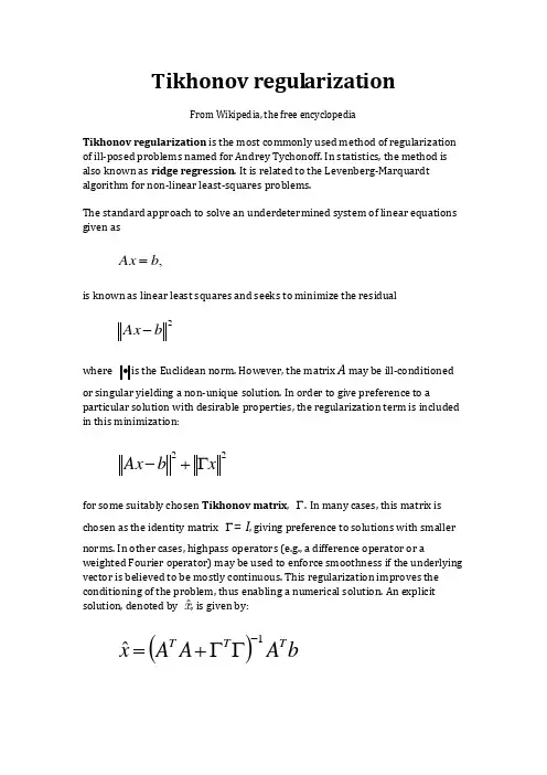
Tikhonov regularizationFrom Wikipedia, the free encyclopediaTikhonov regularization is the most commonly used method of regularization of ill-posed problems named for Andrey Tychonoff. In statistics, the method is also known as ridge regression . It is related to the Levenberg-Marquardt algorithm for non-linear least-squares problems.The standard approach to solve an underdetermined system of linear equations given as,b Ax = is known as linear least squares and seeks to minimize the residual2b Ax -where ∙is the Euclidean norm. However, the matrix A may be ill-conditioned or singular yielding a non-unique solution. In order to give preference to a particular solution with desirable properties, the regularization term is included in this minimization:22x b Ax Γ+-for some suitably chosen Tikhonov matrix , Γ. In many cases, this matrix is chosen as the identity matrix Γ= I , giving preference to solutions with smaller norms. In other cases, highpass operators (e.g., a difference operator or aweighted Fourier operator) may be used to enforce smoothness if the underlying vector is believed to be mostly continuous. This regularization improves the conditioning of the problem, thus enabling a numerical solution. An explicit solution, denoted by , is given by:()b A A A x T T T 1ˆ-ΓΓ+=The effect of regularization may be varied via the scale of matrix Γ. For Γ= αI, when α = 0 this reduces to the unregularized least squares solution provided that (A T A)−1 exists.Contents∙ 1 Bayesian interpretation∙ 2 Generalized Tikhonov regularization∙ 3 Regularization in Hilbert space∙ 4 Relation to singular value decomposition and Wiener filter∙ 5 Determination of the Tikhonov factor∙ 6 Relation to probabilistic formulation∙7 History∙8 ReferencesBayesian interpretationAlthough at first the choice of the solution to this regularized problem may look artificial, and indeed the matrix Γseems rather arbitrary, the process can be justified from a Bayesian point of view. Note that for an ill-posed problem one must necessarily introduce some additional assumptions in order to get a stable solution. Statistically we might assume that a priori we know that x is a random variable with a multivariate normal distribution. For simplicity we take the mean to be zero and assume that each component is independent with standard deviation σx. Our data is also subject to errors, and we take the errors in b to bealso independent with zero mean and standard deviation σb. Under these assumptions the Tikhonov-regularized solution is the most probable solutiongiven the data and the a priori distribution of x, according to Bayes' theorem. The Tikhonov matrix is then Γ= αI for Tikhonov factor α = σb/ σx.If the assumption of normality is replaced by assumptions of homoskedasticity and uncorrelatedness of errors, and still assume zero mean, then theGauss-Markov theorem entails that the solution is minimal unbiased estimate.Generalized Tikhonov regularizationFor general multivariate normal distributions for x and the data error, one can apply a transformation of the variables to reduce to the case above. Equivalently, one can seek an x to minimize22Q P x x b Ax -+- where we have used 2P x to stand for the weighted norm x T Px (cf. theMahalanobis distance). In the Bayesian interpretation P is the inverse covariance matrix of b , x 0 is the expected value of x , and Q is the inverse covariance matrix of x . The Tikhonov matrix is then given as a factorization of the matrix Q = ΓT Γ(e.g. the cholesky factorization), and is considered a whitening filter. This generalized problem can be solved explicitly using the formula()()010Ax b P A Q PA A x T T -++-[edit] Regularization in Hilbert spaceTypically discrete linear ill-conditioned problems result as discretization of integral equations, and one can formulate Tikhonov regularization in the original infinite dimensional context. In the above we can interpret A as a compact operator on Hilbert spaces, and x and b as elements in the domain and range of A . The operator ΓΓ+T A A *is then a self-adjoint bounded invertible operator.Relation to singular value decomposition and Wiener filterWith Γ = αI , this least squares solution can be analyzed in a special way via the singular value decomposition. Given the singular value decomposition of AT V U A ∑=with singular values σi , the Tikhonov regularized solution can be expressed asb VDU x T =ˆwhere D has diagonal values22ασσ+=i iii Dand is zero elsewhere. This demonstrates the effect of the Tikhonov parameter on the condition number of the regularized problem. For the generalized case a similar representation can be derived using a generalized singular value decomposition. Finally, it is related to the Wiener filter:∑==q i i i T i i v b u f x1ˆσ where the Wiener weights are 222ασσ+=i i i f and q is the rank of A . Determination of the Tikhonov factorThe optimal regularization parameter α is usually unknown and often in practical problems is determined by an ad hoc method. A possible approach relies on the Bayesian interpretation described above. Other approaches include the discrepancy principle, cross-validation, L-curve method, restricted maximum likelihood and unbiased predictive risk estimator. Grace Wahba proved that the optimal parameter, in the sense of leave-one-out cross-validation minimizes: ()()[]21222ˆT T X I X X X I Tr y X RSSG -+--==αβτwhereis the residual sum of squares andτ is the effective number degreeof freedom. Using the previous SVD decomposition, we can simplify the above expression: ()()21'22221'∑∑==++-=q i i i i qi i iu b u u b u y RSS ασα ()21'2220∑=++=qi i i i u b u RSS RSS ασαand ∑∑==++-=+-=q i i qi i i q m m 12221222ασαασστ Relation to probabilistic formulationThe probabilistic formulation of an inverse problem introduces (when all uncertainties are Gaussian) a covariance matrix C M representing the a priori uncertainties on the model parameters, and a covariance matrix C D representing the uncertainties on the observed parameters (see, for instance, Tarantola, 2004[1]). In the special case when these two matrices are diagonal and isotropic,and , and, in this case, the equations of inverse theory reduce to the equations above, with α = σD/ σM.HistoryTikhonov regularization has been invented independently in many different contexts. It became widely known from its application to integral equations from the work of A. N. Tikhonov and D. L. Phillips. Some authors use the term Tikhonov-Phillips regularization. The finite dimensional case was expounded by A. E. Hoerl, who took a statistical approach, and by M. Foster, who interpreted this method as a Wiener-Kolmogorov filter. Following Hoerl, it is known in the statistical literature as ridge regression.[edit] References∙Tychonoff, Andrey Nikolayevich (1943). "Об устойчивости обратных задач [On the stability of inverse problems]". Doklady Akademii NaukSSSR39 (5): 195–198.∙Tychonoff, A. N. (1963). "О решении некорректно поставленных задач и методе регуляризации [Solution of incorrectly formulated problemsand the regularization method]". Doklady Akademii Nauk SSSR151:501–504.. Translated in Soviet Mathematics4: 1035–1038.∙Tychonoff, A. N.; V. Y. Arsenin (1977). Solution of Ill-posed Problems.Washington: Winston & Sons. ISBN 0-470-99124-0.∙Hansen, P.C., 1998, Rank-deficient and Discrete ill-posed problems, SIAM ∙Hoerl AE, 1962, Application of ridge analysis to regression problems, Chemical Engineering Progress, 58, 54-59.∙Foster M, 1961, An application of the Wiener-Kolmogorov smoothing theory to matrix inversion, J. SIAM, 9, 387-392∙Phillips DL, 1962, A technique for the numerical solution of certain integral equations of the first kind, J Assoc Comput Mach, 9, 84-97∙Tarantola A, 2004, Inverse Problem Theory (free PDF version), Society for Industrial and Applied Mathematics, ISBN 0-89871-572-5 ∙Wahba, G, 1990, Spline Models for Observational Data, Society for Industrial and Applied Mathematics。

奈斯派索特点奈斯派索特（Naïve Bayes）是一种基于贝叶斯定理的机器学习算法，常用于文本分类、垃圾邮件过滤、情感分析等任务。

它的核心思想是假设特征之间相互独立，通过计算后验概率来进行分类。

在本文中，我将详细介绍奈斯派索特的特点，并进一步探讨其应用领域和实现原理。

奈斯派索特的一个显著特点是其简单性和高效性。

相对于其他复杂的机器学习算法，奈斯派索特只需要估计先验概率和条件概率，计算简单且速度快。

这使得奈斯派索特在大规模数据集上具有较高的可扩展性和实时性。

同时，奈斯派索特对数据的预处理要求较低，可以处理包含大量特征的高维数据。

奈斯派索特假设特征之间相互独立。

这是一个较强的假设，也是奈斯派索特算法的一个局限性。

在实际情况中，很多特征之间可能存在相关性，违背了独立性的假设。

然而，奈斯派索特在很多实际问题中仍能取得良好的效果，这是因为即使在特征相关的情况下，奈斯派索特的整体性能仍然是可以接受的。

奈斯派索特适用于多类别分类任务。

它可以通过计算每个类别的后验概率来判断样本属于哪个类别。

这使得奈斯派索特在文本分类、垃圾邮件过滤等任务中有着广泛的应用。

同时，奈斯派索特还可以用于预测连续值的回归问题，通过将连续值离散化为不同的类别进行处理。

奈斯派索特对于缺失数据和噪声的鲁棒性较强。

在训练过程中，奈斯派索特可以自动忽略缺失的特征或数据，并且由于其简单的计算方式，噪声对结果的影响相对较小。

这使得奈斯派索特在实际应用中更加稳定可靠。

奈斯派索特的实现原理基于贝叶斯定理。

贝叶斯定理描述了在已知先验概率的情况下，如何更新为后验概率。

在奈斯派索特中，先验概率表示在不考虑任何特征的情况下，每个类别出现的概率；而条件概率表示在已知特征的情况下，每个类别出现的概率。

通过计算先验概率和条件概率，奈斯派索特可以计算出样本属于每个类别的后验概率，并选择具有最高后验概率的类别作为预测结果。

为了计算条件概率，奈斯派索特通常采用朴素的假设，即认为特征之间相互独立。

一、字母顺序表 (1)二、常用的数学英语表述 (7)三、代数英语（高端） (13)一、字母顺序表1、数学专业词汇Aabsolute value 绝对值 accept 接受 acceptable region 接受域additivity 可加性 adjusted 调整的 alternative hypothesis 对立假设analysis 分析 analysis of covariance 协方差分析 analysis of variance 方差分析 arithmetic mean 算术平均值 association 相关性 assumption 假设 assumption checking 假设检验availability 有效度average 均值Bbalanced 平衡的 band 带宽 bar chart 条形图beta-distribution 贝塔分布 between groups 组间的 bias 偏倚 binomial distribution 二项分布 binomial test 二项检验Ccalculate 计算 case 个案 category 类别 center of gravity 重心 central tendency 中心趋势 chi-square distribution 卡方分布 chi-square test 卡方检验 classify 分类cluster analysis 聚类分析 coefficient 系数 coefficient of correlation 相关系数collinearity 共线性 column 列 compare 比较 comparison 对照 components 构成，分量compound 复合的 confidence interval 置信区间 consistency 一致性 constant 常数continuous variable 连续变量 control charts 控制图 correlation 相关 covariance 协方差 covariance matrix 协方差矩阵 critical point 临界点critical value 临界值crosstab 列联表cubic 三次的，立方的 cubic term 三次项 cumulative distribution function 累加分布函数 curve estimation 曲线估计Ddata 数据default 默认的definition 定义deleted residual 剔除残差density function 密度函数dependent variable 因变量description 描述design of experiment 试验设计 deviations 差异 df.(degree of freedom) 自由度 diagnostic 诊断dimension 维discrete variable 离散变量discriminant function 判别函数discriminatory analysis 判别分析distance 距离distribution 分布D-optimal design D-优化设计Eeaqual 相等 effects of interaction 交互效应 efficiency 有效性eigenvalue 特征值equal size 等含量equation 方程error 误差estimate 估计estimation of parameters 参数估计estimations 估计量evaluate 衡量exact value 精确值expectation 期望expected value 期望值exponential 指数的exponential distributon 指数分布 extreme value 极值F factor 因素，因子 factor analysis 因子分析 factor score 因子得分 factorial designs 析因设计factorial experiment 析因试验fit 拟合fitted line 拟合线fitted value 拟合值 fixed model 固定模型 fixed variable 固定变量 fractional factorial design 部分析因设计 frequency 频数 F-test F检验 full factorial design 完全析因设计function 函数Ggamma distribution 伽玛分布 geometric mean 几何均值 group 组Hharmomic mean 调和均值 heterogeneity 不齐性histogram 直方图 homogeneity 齐性homogeneity of variance 方差齐性 hypothesis 假设 hypothesis test 假设检验Iindependence 独立 independent variable 自变量independent-samples 独立样本 index 指数 index of correlation 相关指数 interaction 交互作用 interclass correlation 组内相关 interval estimate 区间估计 intraclass correlation 组间相关 inverse 倒数的iterate 迭代Kkernal 核 Kolmogorov-Smirnov test柯尔莫哥洛夫-斯米诺夫检验 kurtosis 峰度Llarge sample problem 大样本问题 layer 层least-significant difference 最小显著差数 least-square estimation 最小二乘估计 least-square method 最小二乘法 level 水平 level of significance 显著性水平 leverage value 中心化杠杆值 life 寿命 life test 寿命试验 likelihood function 似然函数 likelihood ratio test 似然比检验linear 线性的 linear estimator 线性估计linear model 线性模型 linear regression 线性回归linear relation 线性关系linear term 线性项logarithmic 对数的logarithms 对数 logistic 逻辑的 lost function 损失函数Mmain effect 主效应 matrix 矩阵 maximum 最大值 maximum likelihood estimation 极大似然估计 mean squared deviation(MSD) 均方差 mean sum of square 均方和 measure 衡量 media 中位数 M-estimator M估计minimum 最小值 missing values 缺失值 mixed model 混合模型 mode 众数model 模型Monte Carle method 蒙特卡罗法 moving average 移动平均值multicollinearity 多元共线性multiple comparison 多重比较 multiple correlation 多重相关multiple correlation coefficient 复相关系数multiple correlation coefficient 多元相关系数 multiple regression analysis 多元回归分析multiple regression equation 多元回归方程 multiple response 多响应 multivariate analysis 多元分析Nnegative relationship 负相关 nonadditively 不可加性 nonlinear 非线性 nonlinear regression 非线性回归 noparametric tests 非参数检验 normal distribution 正态分布null hypothesis 零假设 number of cases 个案数Oone-sample 单样本 one-tailed test 单侧检验 one-way ANOVA 单向方差分析 one-way classification 单向分类 optimal 优化的optimum allocation 最优配制 order 排序order statistics 次序统计量 origin 原点orthogonal 正交的 outliers 异常值Ppaired observations 成对观测数据paired-sample 成对样本parameter 参数parameter estimation 参数估计 partial correlation 偏相关partial correlation coefficient 偏相关系数 partial regression coefficient 偏回归系数 percent 百分数percentiles 百分位数 pie chart 饼图 point estimate 点估计 poisson distribution 泊松分布polynomial curve 多项式曲线polynomial regression 多项式回归polynomials 多项式positive relationship 正相关 power 幂P-P plot P-P概率图predict 预测predicted value 预测值prediction intervals 预测区间principal component analysis 主成分分析 proability 概率 probability density function 概率密度函数 probit analysis 概率分析 proportion 比例Qqadratic 二次的 Q-Q plot Q-Q概率图 quadratic term 二次项 quality control 质量控制 quantitative 数量的，度量的 quartiles 四分位数Rrandom 随机的 random number 随机数 random number 随机数 random sampling 随机取样random seed 随机数种子 random variable 随机变量 randomization 随机化 range 极差rank 秩 rank correlation 秩相关 rank statistic 秩统计量 regression analysis 回归分析regression coefficient 回归系数regression line 回归线reject 拒绝rejection region 拒绝域 relationship 关系 reliability 可*性 repeated 重复的report 报告，报表 residual 残差 residual sum of squares 剩余平方和 response 响应risk function 风险函数 robustness 稳健性 root mean square 标准差 row 行 run 游程run test 游程检验Sample 样本 sample size 样本容量 sample space 样本空间 sampling 取样 sampling inspection 抽样检验 scatter chart 散点图 S-curve S形曲线 separately 单独地 sets 集合sign test 符号检验significance 显著性significance level 显著性水平significance testing 显著性检验 significant 显著的，有效的 significant digits 有效数字 skewed distribution 偏态分布 skewness 偏度 small sample problem 小样本问题 smooth 平滑 sort 排序 soruces of variation 方差来源 space 空间 spread 扩展square 平方 standard deviation 标准离差 standard error of mean 均值的标准误差standardization 标准化 standardize 标准化 statistic 统计量 statistical quality control 统计质量控制 std. residual 标准残差 stepwise regression analysis 逐步回归 stimulus 刺激 strong assumption 强假设 stud. deleted residual 学生化剔除残差stud. residual 学生化残差 subsamples 次级样本 sufficient statistic 充分统计量sum 和 sum of squares 平方和 summary 概括，综述Ttable 表t-distribution t分布test 检验test criterion 检验判据test for linearity 线性检验 test of goodness of fit 拟合优度检验 test of homogeneity 齐性检验 test of independence 独立性检验 test rules 检验法则 test statistics 检验统计量 testing function 检验函数 time series 时间序列 tolerance limits 容许限total 总共，和 transformation 转换 treatment 处理 trimmed mean 截尾均值 true value 真值 t-test t检验 two-tailed test 双侧检验Uunbalanced 不平衡的 unbiased estimation 无偏估计 unbiasedness 无偏性 uniform distribution 均匀分布Vvalue of estimator 估计值 variable 变量 variance 方差 variance components 方差分量 variance ratio 方差比 various 不同的 vector 向量Wweight 加权，权重 weighted average 加权平均值 within groups 组内的ZZ score Z分数2. 最优化方法词汇英汉对照表Aactive constraint 活动约束 active set method 活动集法 analytic gradient 解析梯度approximate 近似 arbitrary 强制性的 argument 变量 attainment factor 达到因子Bbandwidth 带宽 be equivalent to 等价于 best-fit 最佳拟合 bound 边界Ccoefficient 系数 complex-value 复数值 component 分量 constant 常数 constrained 有约束的constraint 约束constraint function 约束函数continuous 连续的converge 收敛 cubic polynomial interpolation method三次多项式插值法 curve-fitting 曲线拟合Ddata-fitting 数据拟合 default 默认的，默认的 define 定义 diagonal 对角的 direct search method 直接搜索法 direction of search 搜索方向 discontinuous 不连续Eeigenvalue 特征值 empty matrix 空矩阵 equality 等式 exceeded 溢出的Ffeasible 可行的 feasible solution 可行解 finite-difference 有限差分 first-order 一阶GGauss-Newton method 高斯-牛顿法 goal attainment problem 目标达到问题 gradient 梯度 gradient method 梯度法Hhandle 句柄 Hessian matrix 海色矩阵Independent variables 独立变量inequality 不等式infeasibility 不可行性infeasible 不可行的initial feasible solution 初始可行解initialize 初始化inverse 逆 invoke 激活 iteration 迭代 iteration 迭代JJacobian 雅可比矩阵LLagrange multiplier 拉格朗日乘子 large-scale 大型的 least square 最小二乘 least squares sense 最小二乘意义上的 Levenberg-Marquardt method 列文伯格-马夸尔特法line search 一维搜索 linear 线性的 linear equality constraints 线性等式约束linear programming problem 线性规划问题 local solution 局部解M medium-scale 中型的 minimize 最小化 mixed quadratic and cubic polynomialinterpolation and extrapolation method 混合二次、三次多项式内插、外插法multiobjective 多目标的Nnonlinear 非线性的 norm 范数Oobjective function 目标函数 observed data 测量数据 optimization routine 优化过程optimize 优化 optimizer 求解器 over-determined system 超定系统Pparameter 参数 partial derivatives 偏导数 polynomial interpolation method 多项式插值法Qquadratic 二次的 quadratic interpolation method 二次内插法 quadratic programming 二次规划Rreal-value 实数值 residuals 残差 robust 稳健的 robustness 稳健性，鲁棒性S scalar 标量 semi-infinitely problem 半无限问题 Sequential Quadratic Programming method 序列二次规划法 simplex search method 单纯形法 solution 解 sparse matrix 稀疏矩阵 sparsity pattern 稀疏模式 sparsity structure 稀疏结构 starting point 初始点 step length 步长 subspace trust region method 子空间置信域法 sum-of-squares 平方和 symmetric matrix 对称矩阵Ttermination message 终止信息 termination tolerance 终止容限 the exit condition 退出条件 the method of steepest descent 最速下降法 transpose 转置Uunconstrained 无约束的 under-determined system 负定系统Vvariable 变量 vector 矢量Wweighting matrix 加权矩阵3 样条词汇英汉对照表Aapproximation 逼近 array 数组 a spline in b-form/b-spline b样条 a spline of polynomial piece /ppform spline 分段多项式样条Bbivariate spline function 二元样条函数 break/breaks 断点Ccoefficient/coefficients 系数cubic interpolation 三次插值/三次内插cubic polynomial 三次多项式 cubic smoothing spline 三次平滑样条 cubic spline 三次样条cubic spline interpolation 三次样条插值/三次样条内插 curve 曲线Ddegree of freedom 自由度 dimension 维数Eend conditions 约束条件 input argument 输入参数 interpolation 插值/内插 interval取值区间Kknot/knots 节点Lleast-squares approximation 最小二乘拟合Mmultiplicity 重次 multivariate function 多元函数Ooptional argument 可选参数 order 阶次 output argument 输出参数P point/points 数据点Rrational spline 有理样条 rounding error 舍入误差（相对误差）Sscalar 标量 sequence 数列（数组） spline 样条 spline approximation 样条逼近/样条拟合spline function 样条函数 spline curve 样条曲线 spline interpolation 样条插值/样条内插 spline surface 样条曲面 smoothing spline 平滑样条Ttolerance 允许精度Uunivariate function 一元函数Vvector 向量Wweight/weights 权重4 偏微分方程数值解词汇英汉对照表Aabsolute error 绝对误差 absolute tolerance 绝对容限 adaptive mesh 适应性网格Bboundary condition 边界条件Ccontour plot 等值线图 converge 收敛 coordinate 坐标系Ddecomposed 分解的 decomposed geometry matrix 分解几何矩阵 diagonal matrix 对角矩阵 Dirichlet boundary conditions Dirichlet边界条件Eeigenvalue 特征值 elliptic 椭圆形的 error estimate 误差估计 exact solution 精确解Ggeneralized Neumann boundary condition 推广的Neumann边界条件 geometry 几何形状geometry description matrix 几何描述矩阵 geometry matrix 几何矩阵 graphical user interface（GUI）图形用户界面Hhyperbolic 双曲线的Iinitial mesh 初始网格Jjiggle 微调LLagrange multipliers 拉格朗日乘子Laplace equation 拉普拉斯方程linear interpolation 线性插值 loop 循环Mmachine precision 机器精度 mixed boundary condition 混合边界条件NNeuman boundary condition Neuman边界条件 node point 节点 nonlinear solver 非线性求解器 normal vector 法向量PParabolic 抛物线型的 partial differential equation 偏微分方程 plane strain 平面应变 plane stress 平面应力 Poisson's equation 泊松方程 polygon 多边形 positive definite 正定Qquality 质量Rrefined triangular mesh 加密的三角形网格 relative tolerance 相对容限 relative tolerance 相对容限 residual 残差 residual norm 残差范数Ssingular 奇异的二、常用的数学英语表述1.Logic∃there exist∀for allp⇒q p implies q / if p, then qp⇔q p if and only if q /p is equivalent to q / p and q are equivalent2.Setsx∈A x belongs to A / x is an element (or a member) of Ax∉A x does not belong to A / x is not an element (or a member) of AA⊂B A is contained in B / A is a subset of BA⊃B A contains B / B is a subset of AA∩B A cap B / A meet B / A intersection BA∪B A cup B / A join B / A union BA\B A minus B / the diference between A and BA×B A cross B / the cartesian product of A and B3. Real numbersx+1 x plus onex-1 x minus onex±1 x plus or minus onexy xy / x multiplied by y(x - y)(x + y) x minus y, x plus yx y x over y= the equals signx = 5 x equals 5 / x is equal to 5x≠5x (is) not equal to 5x≡y x is equivalent to (or identical with) yx ≡ y x is not equivalent to (or identical with) yx > y x is greater than yx≥y x is greater than or equal to yx < y x is less than yx≤y x is less than or equal to y0 < x < 1 zero is less than x is less than 10≤x≤1zero is less than or equal to x is less than or equal to 1| x | mod x / modulus xx 2 x squared / x (raised) to the power 2x 3 x cubedx 4 x to the fourth / x to the power fourx n x to the nth / x to the power nx −n x to the (power) minus nx (square) root x / the square root of xx 3 cube root (of) xx 4 fourth root (of) xx n nth root (of) x( x+y ) 2 x plus y all squared( x y ) 2 x over y all squaredn! n factorialx ^ x hatx ¯ x barx ˜x tildex i xi / x subscript i / x suffix i / x sub i∑ i=1 n a i the sum from i equals one to n a i / the sum as i runs from 1 to n of the a i4. Linear algebra‖ x ‖the norm (or modulus) of xOA →OA / vector OAOA ¯ OA / the length of the segment OAA T A transpose / the transpose of AA −1 A inverse / the inverse of A5. Functionsf( x ) fx / f of x / the function f of xf:S→T a function f from S to Tx→y x maps to y / x is sent (or mapped) to yf'( x ) f prime x / f dash x / the (first) derivative of f with respect to xf''( x ) f double-prime x / f double-dash x / the second derivative of f with r espect to xf'''( x ) triple-prime x / f triple-dash x / the third derivative of f with respect to xf (4) ( x ) f four x / the fourth derivative of f with respect to x∂f ∂ x 1the partial (derivative) of f with respect to x1∂ 2 f ∂ x 1 2the second partial (derivative) of f with respect to x1∫ 0 ∞the integral from zero to infinitylim⁡x→0 the limit as x approaches zerolim⁡x→0 + the limit as x approaches zero from abovelim⁡x→0 −the limit as x approaches zero from belowlog e y log y to the base e / log to the base e of y / natural log (of) yln⁡y log y to the base e / log to the base e of y / natural log (of) y一般词汇数学mathematics, maths(BrE), math(AmE)公理axiom定理theorem计算calculation运算operation证明prove假设hypothesis, hypotheses(pl.)命题proposition算术arithmetic加plus(prep.), add(v.), addition(n.)被加数augend, summand加数addend和sum减minus(prep.), subtract(v.), subtraction(n.)被减数minuend减数subtrahend差remainder乘times(prep.), multiply(v.), multiplication(n.)被乘数multiplicand, faciend乘数multiplicator积product除divided by(prep.), divide(v.), division(n.)被除数dividend除数divisor商quotient等于equals, is equal to, is equivalent to 大于is greater than小于is lesser than大于等于is equal or greater than小于等于is equal or lesser than运算符operator数字digit数number自然数natural number整数integer小数decimal小数点decimal point分数fraction分子numerator分母denominator比ratio正positive负negative零null, zero, nought, nil十进制decimal system二进制binary system十六进制hexadecimal system权weight, significance进位carry截尾truncation四舍五入round下舍入round down上舍入round up有效数字significant digit无效数字insignificant digit代数algebra公式formula, formulae(pl.)单项式monomial多项式polynomial, multinomial系数coefficient未知数unknown, x-factor, y-factor, z-factor 等式，方程式equation一次方程simple equation二次方程quadratic equation三次方程cubic equation四次方程quartic equation不等式inequation阶乘factorial对数logarithm指数，幂exponent乘方power二次方，平方square三次方，立方cube四次方the power of four, the fourth power n次方the power of n, the nth power开方evolution, extraction二次方根，平方根square root三次方根，立方根cube root四次方根the root of four, the fourth root n次方根the root of n, the nth root集合aggregate元素element空集void子集subset交集intersection并集union补集complement映射mapping函数function定义域domain, field of definition值域range常量constant变量variable单调性monotonicity奇偶性parity周期性periodicity图象image数列，级数series微积分calculus微分differential导数derivative极限limit无穷大infinite(a.) infinity(n.)无穷小infinitesimal积分integral定积分definite integral不定积分indefinite integral有理数rational number无理数irrational number实数real number虚数imaginary number复数complex number矩阵matrix行列式determinant几何geometry点point线line面plane体solid线段segment射线radial平行parallel相交intersect角angle角度degree弧度radian锐角acute angle直角right angle钝角obtuse angle平角straight angle周角perigon底base边side高height三角形triangle锐角三角形acute triangle直角三角形right triangle直角边leg斜边hypotenuse勾股定理Pythagorean theorem钝角三角形obtuse triangle不等边三角形scalene triangle等腰三角形isosceles triangle等边三角形equilateral triangle四边形quadrilateral平行四边形parallelogram矩形rectangle长length宽width附：在一个分数里，分子或分母或两者均含有分数。

R的应用领域包介绍 By R-FoxAnalysis of Pharmacokinetic Data 药物（代谢）动力学数据分析网址：/web/views/Pharmacokinetics.html维护人员：Suzette Blanchard版本：2008-02-15翻译：R-fox, 2008-04-12药物（代谢）动力学数据分析的主要目的是用非线性浓度时间曲线（concentration time curve）或相关的总结（如曲线下面积）确定给药方案（dosing regimen）和身体对药物反应间的关系。

R基本包里的nls()函数用非线性最小二乘估计法估计非线性模型的参数，返回nls类的对象，有 coef()，formula()， resid()，print()， summary()，AIC()，fitted() and vcov()等方法。

在主要目的实现后，兴趣就转移到研究属性（如：年龄、体重、伴随用药、肾功能）不同的人群是否需要改变药物剂量。

在药物（代谢）动力学领域，分析多个个体的组合数据估计人群参数被称作群体药动学（population PK）。

非线性混合模型为分析群体药动学数据提供了自然的工具，包括概率或贝叶斯估计方法。

nlme包用Lindstrom和Bates提出的概率方法拟合非线性混合效应模型(1990, Biometrics 46, 673-87)，允许nested随机效应（nested random effects），组内误差允许相关的或不等的方差。

返回一个nlme类的对象表示拟合结果，结果可用print()，plot()和summary() 方法输出。

nlme对象给出了细节的结果信息和提取方法。

nlmeODE包组合odesolve包和nlme包做混合效应建模，包括多个药动学/药效学(PK/PD)模型。

面版数据(panel data)的贝叶斯估计方法在CRAN的Bayesian Inference任务列表里有所描述（/web/views/Bayesian.html）。

莱文斯坦聚类算法-概述说明以及解释1.引言1.1 概述莱文斯坦聚类算法是一种基于字符串相似度的聚类方法，通过计算字符串之间的莱文斯坦距离来确定它们的相似程度，进而将相似的字符串聚合在一起。

与传统的基于欧氏距离或余弦相似度的聚类方法不同，莱文斯坦距离考虑了字符串之间的编辑操作数量，使得算法在处理拼写错误或简单文本转换时具有更好的鲁棒性。

本文将介绍莱文斯坦聚类算法的原理及其应用场景，探讨其优缺点，并展望未来在文本数据处理和信息检索领域的潜在发展。

通过深入了解和研究莱文斯坦聚类算法，读者将能够更好地理解文本数据处理中的聚类技术，为实际应用提供有益的参考和指导。

1.2 文章结构本文主要分为引言、正文和结论三个部分。

在引言部分中，将介绍莱文斯坦聚类算法的概述、文章结构和目的。

在正文部分将详细介绍什么是莱文斯坦聚类算法、莱文斯坦距离的概念以及莱文斯坦聚类算法的应用。

最后，结论部分将对整篇文章进行总结，评述算法的优缺点，并展望未来在该领域的发展方向。

通过这样的结构，读者可以全面了解莱文斯坦聚类算法的原理、应用以及未来发展前景。

1.3 目的莱文斯坦聚类算法是一种基于编辑距离的聚类方法，旨在利用文本、字符串等数据之间的相似度来实现有效的聚类。

本文旨在介绍莱文斯坦聚类算法的原理、应用和优缺点，帮助读者了解该算法在数据挖掘和文本处理领域的重要性和应用价值。

通过深入探讨莱文斯坦距离的概念和莱文斯坦聚类算法的实际应用案例，读者可以更加全面地了解该算法的工作原理和效果。

同时，本文还将评述莱文斯坦聚类算法的优缺点，并展望未来该算法在数据处理和信息检索领域的发展方向和潜力，为读者提供对该算法的全面认识和深入理解。

2.正文2.1 什么是莱文斯坦聚类算法：莱文斯坦聚类算法是一种基于字符串相似度的聚类算法。

在传统的聚类算法中，通常是通过计算样本之间的距离来进行聚类，而莱文斯坦聚类算法则是通过计算字符串之间的相似度来进行聚类。

莱文斯坦距离是用来衡量两个字符串之间的相似度的一种指标。

浅谈高光谱图像融合方法作者：洪科汤漫来源：《科技风》2019年第16期摘要：高光谱图像有着丰富的光谱信息，能够更好的反映地物的实际情况，但是高光谱图像空间分辨率比较低，所以提高高光谱圖像的空间分辨率有着极大的作用。

高光谱图像融合是改善其图像质量的重要途径。

关键词：高光谱图像;空间分辨率;融合1 基于贝叶斯的方法N.Akhtar等人[1]通过考虑将获取的高分辨率图像空间信息与低分辨率的高光谱图像进行融合，提升高光谱图像的空间分辨率。

基于该思路，通过非参数贝叶斯稀疏表示将高光谱图像与高分辨率图像融合，联合利用图像的空间结构信息以及高光谱图像的光谱域信息，避免重建图像的光谱失真问题。

该方法首先估计场景中材料反射光谱的概率分布以及一组伯努利分布;其次，通过贝叶斯字典学习得到光谱字典，并根据高分辨率图像的频谱量化进行字典变换;然后，利用变换后的字典，通过贝叶斯稀疏编码策略计算高分辨率图像的稀疏编码矩阵;最后，将贝叶斯学习的字典与稀疏编码矩阵联合重建高分辨率的高光谱图像。

实验结果分析表明，本方法在主观视觉方面，图像的细节信息更加清晰，客观指标上RMSE 和 PSNR 的值也优于其他稀疏表示方法。

2 基于矩阵分解的方法R.KAWAKAMI等人[2]提出首先利用光谱分解问题的一个有原则的解，得到了一组表示场景中各种材料反射率的最优基函数。

由于基于高光谱图像中每个像素可能只有少量材料的简单观察，我们将解混问题转化为稀疏矩阵分解问题，并通过“L1-极小化”求解。

在此基础上，结合高分辨率的RGB观测结果，重建了每个位置的光谱。

该方法在高分辨率RGB相机与低分辨率相机之间存在较大的分辨率差距的情况下，能够有效地获得非常精确的光谱估计。

3 基于深度学习的方法Renwei Dian等人[3]提出不同于HSI的先验模型，HSI锐化方法首先直接利用基于CNN残差学习的先验知识，可以较好地模拟HR-HSIs的先验知识。

然后将先验知识通过基于深度神经网络的残差学习引入融合框架。

sklearn的聚类指标聚类是一种常见的无监督学习方法，用于将相似的数据样本分组或分类。

在sklearn中，提供了多种聚类算法和相应的聚类指标来评估聚类结果的质量。

本文将介绍sklearn中常用的聚类指标，包括轮廓系数、Calinski-Harabasz指数和Davies-Bouldin指数。

一、轮廓系数（Silhouette Coefficient）轮廓系数是一种用于评估聚类结果的指标，其值介于[-1, 1]之间。

轮廓系数越接近1，表示样本越与其所在的簇相似；轮廓系数越接近-1，表示样本越与其他簇更相似；轮廓系数接近0，则表示样本在两个簇之间的边界上。

计算轮廓系数的步骤如下：1. 对于每一个样本，计算其与同簇内其他样本的平均距离（a）；2. 对于每一个样本，计算其与其他簇内样本的平均距离（b）；3. 对于每一个样本，计算其轮廓系数（s）：s = (b - a) / max(a, b)二、Calinski-Harabasz指数Calinski-Harabasz指数是一种用于评估聚类结果的指标，其值越大表示聚类效果越好。

该指数计算的是簇内的离散程度与簇间的离散程度之比，离散程度越大，指数值越大。

计算Calinski-Harabasz指数的步骤如下：1. 计算每个簇内样本的平均距离（WSS）；2. 计算所有簇内样本的平均距离（BSS）；3. 计算Calinski-Harabasz指数（CH）：CH = (BSS / (k - 1)) / (WSS / (n - k))其中，k为簇的个数，n为样本的总数。

三、Davies-Bouldin指数Davies-Bouldin指数是一种用于评估聚类结果的指标，其值越小表示聚类效果越好。

该指数计算的是簇内样本的紧密度与簇间样本的分离度之和，紧密度越大，分离度越小，指数值越小。

计算Davies-Bouldin指数的步骤如下：1. 计算每个簇内样本的离心度（Scatter）；2. 计算每个簇与其他簇之间的距离（Separation）；3. 计算Davies-Bouldin指数（DB）：DB = (1 / k) * sum(max((Scatter(i) + Scatter(j)) / Separation(i, j)))其中，k为簇的个数。