Electromagnetic Casimir densities for a wedge with a coaxial cylindrical shell
- 格式:pdf
- 大小:443.99 KB
- 文档页数:21
金属材料专业英语Material Science 材料科学Material Science Definition 材料科学定义Machinability [məʃi:nə'biliti] 加工性能Strength .[streŋθ] 强度Corrosion & resistance durability.[kə'rəʊʒən] &[ri'zistəns] .[ 'djʊrə'bɪlətɪ] 抗腐蚀及耐用Special metallic features 金属特性Allergic, re-cycling & environmental protection 抗敏感及环境保护[ə'lə:dʒik]Chemical element 化学元素'elimənt]Atom of Elements 元素的原子序数Atom and solid material 原子及固体物质Atom Constitutes 原子的组织图['kɔnstitju:t]Periodic Table 周期表[,piəri'ɔdik] adj. 周期的;定期的Atom Bonding 原子键结合Metal and Alloy 金属与合金['ælɔi, ə'lɔi]Ferrous & Non Ferrous Metal 铁及非铁金属['ferəs] adj. [化]亚铁的;铁的,含铁的Features of Metal 金属的特性Crystal Pattern 晶体结构['kristəl] n. 水晶;结晶,晶体;水晶饰品adj. 水晶的;透明的,清澈的Crystal structure, Space lattice & Unit cell 晶体结构,定向格子及单位晶格['lætis] n. 格子;格架;晶格vt. 使成格子状X –ray crystal analytics method X线结晶分析法[,ænə'litik,-kəl]Metal space lattice 金属结晶格子Lattice constant 点阵常数Mill's Index 米勒指数Metal Phase and Phase Rule金相及相律Solid solution 固熔体Substitutional type solid solution 置换固熔体[,sʌbstitju:ʃənəl]Interstitial solid solution 间隙固熔体[,intə'stiʃəl]n. 填隙原子;节间adj. 间质的;空隙的;填隙的Intermetallic compound 金属间化合物[,intəmi'tælik] ['k ɔmpaund, kəm'paund]vt. 混合;合成;和解妥协;搀合vi. 妥协;和解n. 化合物;复合词;混合物adj. 复合的;混合的Transformation 转变Transformation Point 转变点Magnetic Transformation 磁性转变[mæɡ'netik] Allotropic Transformation 同素转变[mæɡ'netik] adj. [化]同素异形的Thermal Equilibrium 热平衡['θə:məl] adj. 热的,热量的n. 上升暖气流adj. 热的,热量的[,i:kwi'libriəm] Degree of freedom 自由度Critical temperature 临界温度Eutectic 共晶[ju:'tektik]n. 共熔合金adj. 共熔的;容易溶解的Peritectic [.peri’tektik] Temperature包晶温度Peritectic Reaction 包晶反应Peritectic Alloy 包晶合金Hypoeutectic Alloy 亚共晶体[,haipəuju'tektik]n. 低级低共熔体adj. 亚共晶的Hypereutectic Alloy 过共晶体Plastic Deformation 金属塑性[,di:fɔ:'meiʃən] n. 变形Slip Plan 滑动面Distortion 畸变[dis'tɔ:ʃən]Work Hardening 硬化Annealing 退火Crystal Recovery 回复柔软Recrystallization 再结晶[ri:,kristəlai'zeiʃən]Properties & testing of metal 金属材料的性能及试验Chemical Properties 化学性能['prɔpəti]Physical Properties 物理性能Magnetism 磁性['mæɡnitizəm]Specific resistivity & specific resistance 比电阻Specific gravity & specific density比重Specific Heat比热热膨胀系数Coefficient of thermal expansion['mæɡnitizəm] n. 协同因素;[数]系数;[物]率adj. 合作的;共同作用的['θə:məl] adj. 热的,热量的n. 上升暖气流导热度Heat conductivity机械性能Mechanical properties [mi'kænikəl] adj. 机械的;呆板的;力学的;无意识的;手工操作的屈服强度(降伏强度) (Yield strength)弹性限度、杨氏弹性系数及屈服点elastic limit, Young’s module of elasticity to yield point [i'læstik] adj. 有弹性的;易伸缩的;灵活的n. 松紧带;橡皮圈['mɔdju:l, -dʒu:l] n. 模数;模块;组件[,elæs'tisəti] n. 弹性;弹力;灵活性伸长度[,i:lɔŋ'ɡeiʃən, i,lɔŋ-]断面缩率Reduction of area [ri'dʌkʃən]破坏性检验destructive inspections渗透探伤法Penetrate inspection磁粉探伤法Magnetic particle inspection放射线探伤法Radiographic inspection [,reidiəu'græfik] adj. 射线照相术的超声波探伤法Ultrasonic inspection [,ʌltrə'sɔnik] adj. 超音速的;超声的n. 超声波显微观察法Microscopic inspection [,maikrə'skɔpik]破坏的检验Destructive Inspection冲击测试Impact Test疲劳测试Fatigue Test [fə'ti:ɡ] n. 疲劳,疲乏;杂役vt. 使疲劳;使心智衰弱vi. 疲劳adj. 疲劳的蠕变试验Creep Test [kri:p] vi. 爬行;慢慢地移动;起鸡皮疙瘩;蔓延n. 爬行;毛骨悚然的感觉;谄媚者潜变强度Creeps Strength第一潜变期Primary Creep第二潜变期Secondary Creep第三潜变期Tertiary Creep主要金属元素之物理性质Physical properties of major Metal Elements工业标准及规格–铁及非铁金属Industrial Standard –Ferrous & Non –ferrous Metal磁力Magnetic简介General软磁Soft Magnetic硬磁Hard Magnetic磁场Magnetic Field磁性感应Magnetic Induction导磁率[系数,性] Magnetic Permeability [,pə:miə'biliti] n. 弥漫;渗透性;[物]透磁率,导磁系数磁化率 Magnetic Susceptibility (Xm) [sə,septə'biləti] 磁力(Magnetic Force)及磁场 (Magnetic Field)是因物料里的电子 (Electron)活动而产生抗磁体、顺磁体、铁磁体、反铁磁体及亚铁磁体Diamagnetism, Paramagnetic, Ferromagnetisms, Antiferromagnetism & Ferrimagnetisms 抗磁体 Diamagnetism磁偶极子 Dipole ['daipəul]负磁力效应 Negative effect顺磁体 Paramagnetic正磁化率Positive magnetic susceptibility [sə,septə'biləti]铁磁体 Ferromagnetism转变元素 Transition element交换能量 Positive energy exchange外价电子 Outer valence electrons ['veiləns] n. [化]价;原子价;化合价;[生]效价化学结合 Chemical bond自发上磁 Spontaneous magnetization [spɔn'teiniəs] 磁畴 Magnetic domain [dəu'mein] n. 领域;产业;地产;[计]域名相反旋转 Opposite span ['ɔpəzit, -sit]比较抗磁体、顺磁体及铁磁体 Comparison of Diamagnetism, Paramagnetic & Ferromagnetism反铁磁体 Antiferromagnetism亚铁磁体 Ferrimagnetism磁矩 magnetic moment净磁矩 Net magnetic moment钢铁的主要成份 The major element of steel钢铁用"碳"之含量来分类Classification of Steel according to Carbon contents铁相 Steel Phases ['feisi:z] n. 阶段,时期(phase 的复数形式)v. 逐步实行(phase的三单形式)钢铁的名称 Name of steel铁素体Ferrite ['ferait]渗碳体 Cementitle奥氏体 Austenite珠光体及共析钢 Pearlite &Eutectoid奥氏体碳钢 Austenite Carbon Steel单相金属 Single Phase Metal共释变态 Eutectoid Transformation珠光体 Pearlite亚铁释体 Hyppo-Eutectoid初释纯铁体 Pro-entectoid ferrite过共释钢 Hype-eutectoid [haip] n. 大肆宣传;皮下注射vt. 大肆宣传;使…兴奋粗珠光体 Coarse pearlite [kɔ:s] adj. 粗糙的;下等的;粗俗的中珠光体 Medium Pearlite幼珠光体 Fine pearlite磁性变态点 Magnetic Transformation钢铁的制造Manufacturing of Steel [,mænju'fæktʃəriŋ]连续铸造法 Continuous casting process电炉 Electric furnace均热炉 Soaking pit ['səukiŋ] n. 浸湿,浸透adj. 湿透的,极湿的adv. 湿透地全静钢 Killed steel半静钢 Semi-killed steel沸腾钢(未净钢) Rimmed steel [rim] n. 边,边缘;轮辋;圆圈vi. 作…的边,装边于vt. 作…的边,装边于钢铁生产流程 Steel Production Flow Chart钢材的熔铸、锻造、挤压及延轧 The Casting, Fogging, Extrusion, Rolling & Steel熔铸 Casting锻造 Fogging挤压 Extrusion延轧Rolling冲剪 Drawing & stamping特殊钢以元素分类Classification of Special Steel according to Element特殊钢以用途来分类 Classification of Special Steel according to End Usage 易车(快削)不锈钢 Free Cutting Stainless Steel含铅易车钢 Leaded Free Cutting Steel含硫易车钢 Sulphuric Free Cutting Steel [sʌl'fjuərik]硬化性能 Hardenability钢的脆性 Brittleness of Steel ['britlnis] n. 脆弱性;脆性,脆度低温脆性 Cold brittleness回火脆性 Temper brittleness日工标准下的特殊钢材 Specail Steel according to JIS Standard铬钢–日工标准 JIS G4104 Chrome steel to JIS G4104 铬钼钢钢材–日工标准G4105 62 Chrome Molybdenum steel to JIS G4105 [krəum]镍铬–日工标准 G4102 63 Chrome Nickel steel to JIS G4102 ['nikəl] n. 镍;镍币;五分镍币vt. 镀镍于镍铬钼钢–日工标准G4103 64 Nickel, Chrome & Molybdenum Steel to JIS G4103高锰钢铸–日工标准High manganese steel to JIS standard ['mæŋɡə,ni:s, ,mæŋɡə'ni:z]片及板材 Chapter Four-Strip, Steel & Plate冷辘低碳钢片(双单光片)(日工标准 JIS G3141) 73 - 95 Cold Rolled (Low carbon) Steel Strip (to JIS G 3141) 简介 General美材试标准的冷辘低碳钢片 Cold Rolled Steel Strip American Standard – American Society for testing and materials (ASTM)日工标准 JIS G3141冷辘低碳钢片 (双单光片)的编号浅释 Decoding of cold rolled(Low carbon)steel strip JIS G3141 [,di:'kəudiŋ] n. 译码;解码v. 破译;译解(decode的ing形式)材料的加工性能 Drawing ability硬度 Hardness表面处理 Surface finish冷辘钢捆片及张片制作流程图表 Production flow chart cold rolled steel coil sheet冷辘钢捆片及张片的电镀和印刷方法 Cold rolled steel coil & sheet electro-plating & painting method [kɔil] vt. n. 延长;伸长;延伸率;伸长率盘绕,把…卷成圈n. 卷;线圈vi. 成圈状冷辘(低碳)钢片的分类用途、工业标准、品质、加热状态及硬度表End usages, industrial standard, quality, condition and hardness of cold rolled steel strip 硬度及拉力 Hardness & Tensile strength test ['tensail, -səl] adj. [物]拉力的;可伸长的;可拉长的拉伸测试(顺纹测试) Elongation test [,i:lɔŋ'ɡeiʃən, i,lɔŋ-]杯突测试(厚度: 0.4公厘至 1.6公厘,准确至 0.1公厘 3个试片平均数 ) Erichsen test (Thickness: 0.4mm to 1.6mm, figure round up to 0.1mm)曲面(假曲率) Camber厚度及阔度公差 Tolerance on Thickness & Width平坦度(阔度大于500公厘,标准回火) Flatness (width>500mm, temper: standard)弯度 Camber冷辘钢片储存与处理提示 General advice on handling & storage of cold rolled steel coil & sheet防止生锈 Rust Protection生锈速度表 Speed of rusting焊接 Welding气焊 Gas Welding埋弧焊 Submerged-arc Welding [səb'mə:dʒd] adj. 水下的,在水中的v. 使陷入;潜入水中(submerge的过去分词)电阻焊 Resistance Welding冷辘钢片(拉力: 30-32公斤/平方米)在没有表面处理状态下的焊接状况 Spot welding conditions for bared (free from paint, oxides etc) Cold rolled mild steel sheets(T/S:30-32 Kgf/ µ m2)时间效应(老化)及拉伸应变 Aging & Stretcher Strains 日工标准(JIS G3141)[strein] n. 张力;拉紧;血缘;负担;扭伤vi. 拉紧;尽力vt. 拉紧;滥用;滤去;竭力冷辘钢片化学成份 Chemical composition – cold rolled steel sheet to JIS G3141冷辘钢片的"理论重量"计算方程式 Cold Rolled Steel Sheet – Theoretical mass 日工标准(JIS G3141)冷辘钢片重量列表 Mass of Cold-Rolled Steel Sheet to JIS G3141 冷辘钢片订货需知 [,θiə'retikəl, ,θi:ə-] adj. 理论的;假设的;理论上的;推理的Ordering of cold rolled steel strip/sheet其它日工标准冷轧钢片(用途及编号) JIS standard & application of other cold Rolled Special Steel电镀锌钢片或电解钢片Electro-galvanized Steel Sheet/Electrolytic Zinc Coated Steel Sheet电解/电镀锌大大增强钢片的防锈能力Galvanic Action improving Weather & Corrosion Resistance of the Base Steel Sheet [kə'rəuʒən] n. 腐蚀;腐蚀产生的物质;衰败上漆能力 Paint Adhesion [əd'hi:ʒən] n. 支持;粘附;固守电镀锌钢片的焊接 Welding of Electro-galvanized steel sheet ['ɡælvənaiz] vt. 通电;镀锌;刺激点焊 Spot welding滚焊 Seam welding [si:m] n. 缝;接缝vt. 缝合;接合;使留下伤痕Vi. 裂开;产生裂缝电镀锌(电解)钢片 Electro-galvanized Steel Sheet生产流程 Production Flow Chart常用的镀锌钢片(电解片)的基层金属、用途、日工标准、美材标准及一般厚度 Base metal, application, JIS & ASTM standard, and Normal thickness of galvanized steel sheet锌镀层质量 Zinc Coating Mass [ziŋk]表面处理 Surface Treatment冷轧钢片 Cold-Rolled Steel Sheet/Strip热轧钢片 Hot-Rolled Sheet/Strip电解冷轧钢片厚度公差Thickness Tolerance of Electrolytic Cold-rolled sheet热轧钢片厚度公差 Thickness Tolerance of Hot-rolled sheet冷轧或热轧钢片阔度公差 Width Tolerance of Cold or Hot-rolled sheet长度公差 Length Tolerance理论质量 Theoretical Mass [,θiə'retikəl, ,θi:ə-] 锌镀层质量(两个相同锌镀层厚度) Mass Calculation of coating (For equal coating)/MM锌镀层质量(两个不同锌镀层厚度) Mass Calculation of coating (For differential coating)/MM镀锡薄铁片(白铁皮/马口铁) (日工标准 JIS G3303)简介 General镀锡薄铁片的构造Construction of Electrolytic Tinplate镀锡薄钢片(白铁皮/马日铁)制造过程 Production Process of Electrolytic Tinplate锡层质量 Mass of Tin Coating (JIS G3303-1987)两面均等锡层 Both Side Equally Coated Mass两面不均等锡层 Both Side Different Thickness Coated Mass级别、电镀方法、镀层质量及常用称号Grade, Plating type, Designation of Coating Mass & Common Coating Mass镀层质量标记 Markings & Designations of Differential Coatings硬度 Hardness单相轧压镀锡薄铁片(白铁皮/马口铁) Single-Reduced Tinplate双相辗压镀锡薄钢片(马口铁/白铁皮) Dual-Reduction Tinplate钢的种类 Type of Steel常用尺寸 Commonly Used Size电器用硅 [硅] 钢片 Electrical Steel Sheet简介 General软磁材料 Soft Magnetic Material滞后回线 Narrow Hysteresis矫顽磁力 Coercive Force [kəu'ə:siv] adj. 强制的;高压的;胁迫的硬磁材料 Hard Magnetic Material最大能量积 Maximum Energy Product硅含量对电器用的低碳钢片的最大好处 The Advantage of Using Silicon low Carbon Steel晶粒取向(Grain-Oriented)及非晶粒取向(Non-Oriented) Grain Oriented & Non-Oriented ['ɔ:rientid, 'əu-] adj. 定向的;导向的;以…为方向的v. 调整;确定…的方位;使朝向(orient的过去分词)电器用硅 [硅] 钢片的最终用途及规格 End Usage and Designations of Electrical Steel Strip电器用的硅 [硅] 钢片之分类 Classification of Silicon Steel Sheet for Electrical Use电器用钢片的绝缘涂层Performance of Surface Insulation of Electrical Steel Sheets [,insju'leiʃən, 'insə-] n. 绝缘;隔离,孤立晶粒取向电器用硅钢片主要工业标准International Standard – Grain-Oriented Electrical Steel Silicon Steel Sheet for Electrical Use晶粒取向电器用硅钢片 Grain-Oriented Electrical Steel 晶粒取向,定取向芯钢片及高硼定取向芯钢片之磁力性能及夹层系数 (日工标准及美材标准) Magnetic Properties and Lamination Factor of SI-ORIENT-CORE& SI-ORIENT-CORE-HI B Electrical Steel Strip (JIS and AISI Standard)退火 Annealing [ə'ni:l]电器用钢片用家需自行应力退火原因 Annealing of the Electrical Steel Sheet退火时注意事项 Annealing Precautionary碳污染 Prevent Carbon Contamination [kən,tæmi'neiʃən] n. 污染,玷污;污染物热力应先从工件边缘透入 Heat from the Laminated Stacks Edges ['læmineitid] adj. 层压的;层积的;薄板状的v. 分成薄片;用薄片覆盖(laminate的过去分词)提防过份氧化 No Excessive Oxidation [ik'sesiv] [,ɔksi'deiʃən]应力退火温度Stress –relieving Annealing Temperature绝缘表面 Surface Insulation非晶粒取向电力用钢片的电力、磁力、机械性能及夹层系数Lamination Factors of Electrical, Magnetic & Mechanical Non-Grain Oriented Electrical电器及家电外壳用镀层冷辘 [低碳] 钢片 Coated (Low Carbon) Steel Sheets for Casing,Electricals & Home Appliances镀铝硅钢片 Aluminized Silicon Alloy Steel Sheet镀铝硅合金钢片的特色 Feature of Aluminized Silicon Alloy Steel Sheet用途 End Usages抗化学品能力 Chemical Resistance镀铝(硅)钢片–日工标准(JIS G3314) Hot-aluminum-coated sheets and coils to JIS G 3314 镀铝(硅)钢片–美材试标准 (ASTM A-463-77)35.7 JIS G3314镀热浸铝片的机械性能 Mechanical Properties of JIS G 3314 Hot-Dip Aluminum-coated Sheets and Coils公差 Size Tolerance镀铝(硅)钢片及其它种类钢片的抗腐蚀性能比较Comparsion of various resistance of aluminized steel & other kinds of steel镀铝(硅)钢片生产流程 Aluminum Steel Sheet, Production Flow Chart焊接能力 Weldability镀铝钢片的焊接状态(比较冷辘钢片) Tips on welding of Aluminized sheet in comparasion with cold rolled steel strip钢板 Steel Plate钢板用途分类及各国钢板的工业标准包括日工标准及美材试标准 Type of steel Plate & Related JIS, ASTM and Other Major Industrial Standards钢板生产流程 Production Flow Chart钢板订货需知 Ordering of Steel Plate不锈钢 Stainless Steel不锈钢的定义 Definition of Stainless Steel不锈钢之分类,耐腐蚀性及耐热性Classification, Corrosion Resistant & Heat Resistance of Stainless Steel [kə'rəuʒən] n. 腐蚀;腐蚀产生的物质;衰败铁铬系不锈钢片Chrome Stainless Steel马氏体不锈钢Martensite Stainless Steel低碳马氏体不锈钢Low Carbon Martensite Stainless Steel含铁体不锈钢Ferrite Stainless Steel镍铬系不锈钢Nickel Chrome Stainless Steel释出硬化不锈钢Precipitation Hardening Stainless Steel [pri,sipi'tei ʃən] n. 坠落;沉淀,沉淀物;鲁莽;冰雹铁锰铝不锈钢Fe / Mn / Al / Stainless Steel不锈钢的磁性Magnetic Property & Stainless Steel不锈钢箔、卷片、片及板之厚度分类Classification of Foil, Strip, Sheet & Plate by Thickness表面保护胶纸Surface protection film不锈钢片材常用代号Designation of SUS Steel Special Use Stainless 表面处理 Surface finish 薄卷片及薄片(0.3至 2.9mm厚之片)机械性能Mechanical Properties of Thin StainlessSteel(Thickness from 0.3mm to 2.9mm) – strip/sheet 不锈钢片机械性能(301, 304, 631, CSP) Mechanical Properties of Spring use Stainless Steel不锈钢–种类,工业标准,化学成份,特点及主要用途Stainless Steel –Type, Industrial Standard, Chemical Composition, Characteristic & end usage of the most commonly used Stainless Steel不锈钢薄片用途例End Usage of Thinner Gauge [ɡeidʒ] n. 计量器;标准尺寸;容量规格vt. 估计;测量;给…定规格不锈钢片、板用途例Examples of End Usages of Strip, Sheet & Plate不锈钢应力退火卷片常用规格名词图解General Specification of Tension Annealed Stainless Steel Strips耐热不锈钢Heat-Resistance Stainless Steel镍铬系耐热不锈钢特性、化学成份、及操作温度Heat-Resistance Stainless Steel铬系耐热钢Chrome Heat Resistance Steel镍铬耐热钢Ni - Cr Heat Resistance Steel超耐热钢Special Heat Resistance Steel抗热超级合金Heat Resistance Super Alloy耐热不锈钢比重表Specific Gravity of Heat –resistance steel plates and sheets stainless steel不锈钢材及耐热钢材标准对照表Stainless and Heat-Resisting Steels发条片 Power Spring Strip发条的分类及材料 Power Spring Strip Classification and Materials上链发条 Wind-up Spring倒后擦发条 Pull Back Power Spring圆面("卜竹")发条 Convex Spring Strip [kɔn'veks] adj. 凸面的;凸圆的n. 凸面体;凸状拉尺发条 Measure Tape魔术手环 Magic Tape魔术手环尺寸图 Drawing of Magic Tap定型发条 Constant Torque Spring定型发条及上炼发条的驱动力 Spring Force of Constant Torque Spring and Wing-up Spring [tɔ:k] n. 转矩,扭矩;项圈,金属领圈定型发条的形状及翻动过程 Shape and Spring Back of Constant Torque Spring定型发条驱动力公式及代号The Formula and Symbol of Constant Torque Spring边缘处理 Edge Finish硬度 Hardness高碳钢化学成份及用途 High Carbon Tool Steel, Chemical Composition and Usage每公斤发条的长度简易公式 The Length of 1 Kg of Spring Steel Strip SK-5 & AISI-301每公斤长的重量 /公斤(阔 100-200公厘) Weight per one meter long (kg) (Width 100-200mm) SK-5 & AISI-301 每公斤之长度 (阔 100-200公厘) Length per one kg (Width 100-200mm) SK-5 & AISI-301每公尺长的重量 /公斤(阔 2.0-10公厘) Weight per one meter long (kg) (Width 2.0-10mm) SK-5 & AISI-301每公斤之长度 (阔 2.0-10公厘) Length per one kg (Width 2.0-10mm)高碳钢片 High Carbon Steel Strip分类 Classification用组织结构分类Classification According to Grain Structure用含碳量分类–即低碳钢、中碳钢及高碳钢Classification According to Carbon Contains弹簧用碳钢片 Carbon Steel Strip For Spring Use冷轧状态 Cold Rolled Strip回火状态 Annealed Strip淬火及回火状态 Hardened & Tempered Strip/ Precision – Quenched Steel Strip贝氏体钢片 Bainite Steel Strip弹簧用碳钢片材之边缘处理 Edge Finished淬火剂 Quenching Media碳钢回火 Tempering回火有低温回火及高温回火Low & High Temperature Tempering高温回火 High Temperature Tempering退火 Annealing完全退火 Full Annealing扩散退火 Diffusion Annealing [di'fju:ʒən] n. 扩散,传播;[物]漫射低温退火 Low Temperature Annealing中途退火 Process Annealing球化退火 Spheroidizing Annealing光辉退火 Bright Annealing淬火 Quenching [kwentʃ] vt. 结束;熄灭,淬火;解渴;冷浸vi. 熄灭;平息时间淬火 Time Quenching奥氏铁孻回火 Austempering马氏铁体淬火 Marquenching高碳钢片用途 End Usage of High Carbon Steel Strip冷轧高碳钢–日本工业标准 Cold-Rolled (Special Steel) Carbon Steel Strip to JIS G3311电镀金属钢片 Plate Metal Strip电镀金属捆片的优点Advantage of Using Plate Metal Strip金属捆片电镀层 Plated Layer of Plated Metal Strip镀镍 Nickel Plated镀铬 Chrome Plated镀黄铜 Brass Plated基层金属 Base Metal of Plated Metal Strip低碳钢或铁基层金属 Iron & Low Carbon as Base Metal 不锈钢基层金属 Stainless Steel as Base Metal铜基层金属 Copper as Base Metal [beis] n. 底部;垒;基础adj. 卑鄙的;低劣的vt. 以…作基础黄铜基层金属 Brass as Base Metal轴承合金 Bearing Alloy轴承合金–日工标准 JIS H 5401 Bearing Alloy to JIS H 5401锡基、铅基及锌基轴承合金比较表 Comparison of Tin base, Lead base and Zinc base alloy for Bearing purpose 易溶合金 Fusible Alloy焊接合金 Soldering and Brazing Alloy软焊 Soldering Alloy软焊合金–日本标准 JIS H 4341 Soldering Alloy to JIS H 4341硬焊 Brazing Alloy其它焊接材料请参阅日工标准目录Other Soldering Material细线材、枝材、棒材 Chapter Five Wire, Rod & Bar线材/枝材材质分类及制成品 Classification and End Products of Wire/Rod铁线(低碳钢线)日工标准 JIS G 3532 Low Carbon Steel Wires ( Iron Wire ) to JIS G 3532光线(低碳钢线),火线 (退火低碳钢线 ),铅水线 (镀锌低碳钢线)及制造钉用低碳钢线之代号、公差及备注 OrdinaryLow Carbon Steel Wire, Annealed Low Carbon Steel Wire, Galvanized low Carbon Steel Wire & Low Carbon Steel Wire for nail manufacturing - classification, Symbol of Grade, Tolerance and Remarks.机械性能 Mechanical Properites锌包层之重量,铜硫酸盐试验之酸洗次数及测试用卷筒直径Weight of Zinc-Coating, Number of Dippings in Cupric Sulphate Test and Diameters of Mandrel Used for Coiling Test冷冲及冷锻用碳钢线枝 Carbon Steel Wire Rods for Cold Heading & Cold Forging (to JIS G3507)级别,代号及化学成份 Classification, Symbol of Grade and Chemical Composition直径公差,偏圆度及脱碳层的平均深度Diameter/ dai'æmitə] Tolerance, Ovality and Average Decarburized Layer Depth冷拉钢枝材 Cold Drawn Carbon Steel Shafting Bar枝材之美工标准,日工标准,用途及化学成份 AISI, JIS End Usage and Chemical Composition of Cold Drawn Carbon Steel Shafting Bar冷拉钢板重量表 Cold Drawn Steel Bar Weight Table高碳钢线枝 High Carbon Steel Wire Rod (to JIS G3506) 冷拉高碳钢线 Hard Drawn High Carbon Steel Wire (to JIS G3521, ISO-84580-1&2)化学成份分析表 Chemical Analysis of Wire Rod线径、公差及机械性能(日本工业标准 G 3521) Mechanical Properties (JIS G 3521)琴线(日本标准 G3522) Piano Wires (to G3522)级别,代号,扭曲特性及可用之线材直径 Classes, symbols, twisting characteristic and applied Wire Diameters 直径,公差及拉力强度 Diameter, Tolerance and Tensile Strength ['twistiŋ] n. 缠绕;旋扭法;扭转;诱骗adj. 缠绕的;曲折的;转动的v. 编成;盘绕;扭曲(twist 的ing形式) ['tensail, -səl] adj. [物]拉力的;可伸长的;可拉长的裂纹之容许深度及脱碳层 Permissible depth of flaw and decarburized layer [pə'misibl] [flɔ:]常用的弹簧不锈钢线-编号,特性,表面处理及化学成份Stainless Spring Wire – National Standard number, Characteristic, Surface finish & Chemical composition 弹簧不锈钢线,线径及拉力列表Stainless Spring Steel, Wire diameter and Tensile strength of Spring Wire处理及表面状况 Finish & Surface各种不锈钢线在不同处理拉力比较表 Tensile Strength of various kinds of Stainless Steel Wire under Different Finish圆径及偏圆度之公差Tolerance of Wire Diameters & Ovality铬镍不锈钢及抗热钢弹簧线材–美国材验学会 ASTM A313 –1987 Chromium –Nickel Stainless and Heat-resisting Steel Spring Wire – ASTM A313 – 1987 化学成份 Chemical Composition机械性能 Mechanical Properties305, 316, 321及347之拉力表Tensile Strength Requirements for Types 305, 316, 321 and 347A1S1-302贰级线材之拉力表Tensile Strength of A1S1-302 Wire日本工业标准–不锈钢的化学成份 (先数字后字母排列) JIS – Chemical Composition of Stainless Steel (in order of number & alphabet)美国工业标准–不锈钢及防热钢材的化学成份 (先数字后字母排列) AISI – Chemical Composition of Stainless Steel & Heat-Resistant Steel(in order of number & alphabet) ['ælfəbit] n. 字母表,字母系统;入门,初步易车碳钢 Free Cutting Carbon Steels (to JIS G4804 ) 化学成份 Chemical composition圆钢枝,方钢枝及六角钢枝之形状及尺寸之公差 Tolerance on Shape and Dimensions for Round Steel Bar, Square Steel Bar, Hexagonal Steel Bar [hek'sæɡənəl] adj. 六边的,六角形的易车(快削)不锈钢 Free Cutting Stainless Steel易车(快削)不锈钢种类 Type of steel易车(快削)不锈钢拉力表Tensile Strength of Free Cutting Wires枝/棒无芯磨公差表(μ) (μ= 1/100 mm) Rod/Bar Centreless Grind Tolerance [ɡraind]vt. 磨碎;磨快vi. 磨碎;折磨n. 磨;苦工作易车不锈钢及易车钢之不同尺寸及硬度比较 Hardness of Different Types & Size of Free Cutting Steel扁线、半圆线及异形线 Flat Wire, Half Round Wire, Shaped Wire and Precision Shaped Fine Wire [pri'siʒən] n. 精确;精度,精密度adj. 精密的,精确的加工方法 Manufacturing Method应用材料 Material Used特点 Characteristic用途End Usages不锈钢扁线及半圆线常用材料 Commonly used materials for Stainless Flat Wire & Half Round Wire扁线公差 Flat Wire Tolerance方线公差 Square Wire Tolerance专业知识材料科学基础常用英语词汇物料科学Material Science物料科学定义Material Science Definition加工性能Machinability强度Strength抗腐蚀及耐用Corrosion & resistance durability金属特性Special metallic features抗敏感及环境保护Allergic, re-cycling & environmental protection化学元素Chemical element元素的原子序数Atom of Elements原子及固体物质Atom and solid material原子的组成、大小、体积和单位图表The size, mass, charge of an atom, and is particles (Pronton,Nentron and Electron)原子的组织图Atom Constitutes周期表Periodic Table原子键结Atom Bonding金属与合金 Metal and Alloy铁及非铁金属Ferrous & Non Ferrous Metal金属的特性Features of Metal晶体结构 Crystal Pattern晶体结构,定向格子及单位晶格Crystal structure, Space lattice & Unit cellX线结晶分析法X – ray crystal analyics method金属结晶格子 Metal space lattice格子常数 Lattice constant米勒指数 Mill's Index金相及相律 Metal Phase and Phase Rule固熔体 Solid solution置换型固熔体 Substitutional type solid solution 插入型固熔体 Interstital solid solution金属间化物 Intermetallic compound金属变态Transformation变态点Transformation Point磁性变态Magnetic Transformation同素变态Allotropic Transformation合金平衡状态Thermal Equilibrium相律Phase Rule自由度Degree of freedom临界温度Critical temperture共晶Eutectic包晶温度 Peritectic Temperature包晶反应 Peritectic Reaction包晶合金 Peritectic Alloy亚共晶体 Hypoeutetic Alloy过共晶体 Hyper-ectectic Alloy金属的相融、相融温度、晶体反应及合金在共晶合金、固熔孻共晶合金及偏晶反应的比较Equilibrium Comparision金属塑性 Plastic Deformation滑动面 Slip Plan畸变 Distortion硬化 Work Hardening退火 Annealing回复柔软 Crystal Recovery再结晶 Recrystallization金属材料的性能及试验Properties & testing of metal化学性能Chemical Properties物理性能Physical Properties颜色Colour磁性Magnetisum比电阻Specific resistivity & specific resistance比重Specific gravity & specific density比热Specific Heat热膨胀系数Coefficient of thermal expansion导热度Heat conductivity机械性能 Mechanical properties屈服强度(降伏强度) (Yield strangth)弹性限度、阳氏弹性系数及屈服点elastic limit, Yeung's module of elasticity to yield point伸长度Elongation断面缩率Reduction of area金属材料的试验方法The Method of Metal inspection 不破坏检验Non – destructive inspections 渗透探伤法Penetrate inspection磁粉探伤法Magnetic particle inspection放射线探伤法Radiographic inspection超声波探伤法Ultrasonic inspection显微观察法Microscopic inspection破坏的检验Destructive Inspection冲击测试Impact Test疲劳测试Fatigue Test潜变测试 Creep Test潜变强度Creeps Strength第壹潜变期Primary Creep第二潜变期Secondary Creep第三潜变期Tertiary Creep主要金属元素之物理性质Physical properties of major Metal Elements工业标准及规格–铁及非铁金属Industrial Standard – Ferrous & Non – ferrous Metal 磁力 Magnetic简介 General软磁 Soft Magnetic硬磁 Hard Magnetic磁场 Magnetic Field磁性感应 Magnetic Induction透磁度 Magnetic Permeability磁化率 Magnetic Susceptibility (Xm)磁力(Magnetic Force)及磁场(Magnetic Field)是因物料里的电子(Electron)活动而产生抗磁体、顺磁体、铁磁体、反铁磁体及亚铁磁体Diamagnetism, Paramagnetic, Ferromagnetism,Antiferromagnetism & Ferrimagnetism 抗磁体 Diamagnetism磁偶极子 Dipole负磁力效应 Negative effect顺磁体 Paramagnetic正磁化率 Positive magnetic susceptibility铁磁体 Ferromagnetism转变元素 Transition element交换能量 Positive energy exchange外价电子 Outer valence electrons化学结合 Chemical bond自发上磁 Spontaneous magnetization磁畴 Magnetic domain相反旋转 Opposite span比较抗磁体、顺磁体及铁磁体Comparison of Diamagnetism, Paramagnetic & Ferromagnetism反铁磁体 Antiferromagnetism亚铁磁体 Ferrimagnetism磁矩 magnetic moment净磁矩 Net magnetic moment钢铁的主要成份The major element of steel钢铁用"碳"之含量来分类Classification of Steel according to Carbon contents 铁相Steel Phases钢铁的名称Name of steel纯铁体Ferrite渗碳体Cementitle奥氏体 Austenite珠光体及共释钢Pearlite &Eutectoid奥氏体碳钢Austenite Carbon Steel单相金属Single Phase Metal共释变态Eutectoid Transformation珠光体 Pearlite亚铁释体Hyppo-Eutectoid初释纯铁体 Pro-entectoid ferrite过共释钢 Hype-eutectoid珠光体Pearlite粗珠光体 Coarse pearlite中珠光体 Medium pearlite幼珠光体 Fine pearlite磁性变态点 Magnetic Transformation 钢铁的制造Manufacturing of Steel连续铸造法 Continuous casting process 电炉 Electric furnace均热炉 Soaking pit全静钢 Killed steel半静钢 Semi-killed steel沸腾钢(未净钢) Rimmed steel钢铁生产流程 Steel Production Flow Chart钢材的熔铸、锻造、挤压及延轧The Casting, Fogging, Extrusion, Rolling & Steel熔铸 Casting锻造 Fogging挤压 Extrusion延轧 Rolling冲剪 Drawing & stamping特殊钢 Special Steel简介General特殊钢以原素分类Classification of Special Steel according to Element 特殊钢以用途来分类Classification of Special Steel according to End Usage 易车(快削)不锈钢Free Cutting Stainless Steel含铅易车钢Leaded Free Cutting Steel含硫易车钢Sulphuric Free Cutting Steel硬化性能Hardenability钢的脆性Brittleness of Steel低温脆性 Cold brittleness回火脆性 Temper brittleness日工标准下的特殊钢材Specail Steel according to JIS Standard铬钢–日工标准 JIS G4104Chrome steel to JIS G4104铬钼钢钢材–日工标准 G4105 62Chrome Molybdenum steel to JIS G4105镍铬–日工标准 G4102 63Chrome Nickel steel to JIS G4102镍铬钼钢–日工标准 G4103 64Nickel, Chrome & Molybdenum Steel to JIS G4103高锰钢铸–日工标准High manganese steel to JIS standard片及板材Chapter Four-Strip, Steel & Plate冷辘低碳钢片(双单光片)(日工标准 JIS G3141) 73 - 95 Cold Rolled (Low carbon) Steel Strip (to JIS G 3141) 简介General美材试标准的冷辘低碳钢片Cold Rolled Steel Strip American Standard – American Society for testing and materials (ASTM)日工标准JIS G3141冷辘低碳钢片(双单光片)的编号浅释Decoding of cold rolled(Low carbon)steel strip JIS G3141材料的加工性能 Drawing abillity硬度 Hardness表面处理 Surface finish冷辘钢捆片及张片制作流程图表Production flow chart cold rolled steel coil sheet 冷辘钢捆片及张片的电镀和印刷方法Cold rolled steel coil & sheet electro-plating & painting method冷辘(低碳)钢片的分类用、途、工业标准、品质、加热状态及硬度表End usages, industrial standard, quality, condition and hardness of cold rolled steel strip硬度及拉力 Hardness & Tensile strength test拉伸测试(顺纹测试)Elongation test杯突测试(厚度: 0.4公厘至1.6公厘,准确至0.1公厘 3个试片平均数)Erichsen test (Thickness: 0.4mm to 1.6mm, figure round up to 0.1mm)曲面(假曲率)Camber厚度及阔度公差 Tolerance on Thickness & Width平坦度(阔度大于500公厘,标准回火)Flatness (width>500mm, temper: standard)弯度 Camber冷辘钢片储存与处理提示General advice on handling & storage of cold rolled steel coil & sheet防止生锈Rust Protection生锈速度表Speed of rusting焊接 Welding气焊 Gas Welding埋弧焊 Submerged-arc Welding电阻焊 Resistance Welding冷辘钢片(拉力: 30-32公斤/平方米)在没有表面处理状态。
English 中文释义A.C magnetic saturation 交流磁饱和Absorbed dose 吸收剂量Absorbed dose rate 吸收剂量率Acceptanc limits 验收范围Acceptance level 验收水平Acceptance standard 验收标准Accumulation test 累积检测Acoustic emission count(emission count)声发射计数(发射计数) Acoustic emission transducer 声发射换能器(声发射传感器)Acoustic emission(AE) 声发射Acoustic holography 声全息术Acoustic impedance 声阻抗Acoustic impedance matching 声阻抗匹配Acoustic impedance method 声阻法Acoustic wave 声波Acoustical lens 声透镜Acoustic—ultrasonic 声-超声(AU)Activation 活化Activity 活度Adequate shielding 安全屏蔽Ampere turns 安匝数Amplitude 幅度Angle beam method 斜射法Angle of incidence 入射角Angle of reflection 反射角Angle of spread 指向角Angle of squint 偏向角Angle probe 斜探头Angstrom unit 埃(A)Area amplitude response curve 面积幅度曲线Area of interest 评定区Arliflcial disconlinuity 人工不连续性Artifact 假缺陷Artificial defect 人工缺陷Artificial discontinuity 标准人工缺陷A-scan A 型扫描A-scope; A-scan A 型显示Attenuation coefficient 衰减系数Attenuator 衰减器Audible leak indicator 音响泄漏指示器Automatic testing 自动检测Autoradiography 自射线照片Avaluation 评定Barium concrete 钡混凝土Barn 靶Base fog 片基灰雾Bath 槽液Bayard- Alpert ionization gage B- A 型电离计Beam 声束Beam ratio 光束比Beam angle 束张角Beam axis 声束轴线Beam index 声束入射点Beam path location 声程定位Beam path; path length 声程Beam spread 声束扩散Betatron 电子感应加速器Bimetallic strip gage 双金属片计Bipolar field 双极磁场Black light filter 黑光滤波器Black light; ultraviolet radiation 黑光Blackbody 黑体Blackbody equivalent temperature 黑体等效温度 Bleakney mass spectrometer 波利克尼质谱仪Bleedout 渗出Bottom echo 底面回波Bottom surface 底面Boundary echo(first) 边界一次回波Bremsstrahlung 轫致辐射Broad-beam condition 宽射束Brush application 刷涂B-scan presenfation B 型扫描显示B-scope; B-scan B 型显示C- scan C 型扫描Calibration,instrument 设备校准Capillary action 毛细管作用Carrier fluid 载液Carry over of penetrate 渗透剂移转Cassette 暗合Cathode 阴极Central conductor method 中心导体法Characteristic curve 特性曲线Characteristic curve of film 胶片特性曲线Characteristic radiation 特征辐射Chemical fog 化学灰雾Cine-radiography 射线(活动)电影摄影术Cintact pads 接触垫Circumferential coils 圆环线圈Circumferential field 周向磁场Circumferential magnetization method 周向磁化法Clean 清理Clean- up 清除Clearing time 定透时间Coercive force 矫顽力Coherence 相干性Coherence length 相干长度(谐波列长度)Coi1,test 测试线圈Coil size 线圈大小Coil spacing 线圈间距Coil technique 线圈技术Coil method 线圈法Coilreference 线圈参考Coincidence discrimination 符合鉴别Cold-cathode ionization gage 冷阴极电离计Collimator 准直器Collimation 准直Collimator 准直器Combined colour comtrast and fluorescent penetrant 着色荧光渗透剂 Compressed air drying 压缩空气干燥Compressional wave 压缩波Compton scatter 康普顿散射Continuous emission 连续发射Continuous linear array 连续线阵Continuous method 连续法Continuous spectrum 连续谱Continuous wave 连续波Contract stretch 对比度宽限Contrast 对比度Contrast agent 对比剂Contrast aid 反差剂Contrast sensitivity 对比灵敏度Control echo 监视回波Control echo 参考回波Couplant 耦合剂Coupling 耦合Coupling losses 耦合损失Cracking 裂解Creeping wave 爬波Critical angle 临界角Cross section 横截面Cross talk 串音Cross-drilled hole 横孔Crystal 晶片C-scope; C-scan C 型显示Curie point 居里点Curie temperature 居里温度Curie(Ci) 居里Current flow method 通电法Current induction method 电流感应法Current magnetization method 电流磁化法Cut-off level 截止电平Dead zone 盲区Decay curve 衰变曲线Decibel(dB) 分贝Defect 缺陷Defect resolution 缺陷分辨力Defect detection sensitivity 缺陷检出灵敏度Defect resolution 缺陷分辨力Definition 清晰度Definition, image definition 清晰度,图像清晰度Demagnetization 退磁Demagnetization factor 退磁因子Demagnetizer 退磁装置Densitometer 黑度计Density 黑度(底片)Density comparison strip 黑度比较片Detecting medium 检验介质Detergent remover 洗净液Developer 显像剂Developer, agueons 水性显象剂Developer, dry 干显象剂Developer, liquid film 液膜显象剂Developer, nonaqueous (sus- pendible)非水(可悬浮)显象剂 Developing time 显像时间Development 显影Diffraction mottle 衍射斑Diffuse indications 松散指示Diffusion 扩散Digital image acquisition system 数字图像识别系统Dilatational wave 膨胀波Dip and drain station 浸渍和流滴工位Direct contact magnetization 直接接触磁化Direct exposure imaging 直接曝光成像Direct contact method 直接接触法Directivity 指向性Discontinuity 不连续性Distance- gain- size-German A VG 距离- 增益- 尺寸(DGS 德文为A VG) Distance marker; time marker 距离刻度Dose equivalent 剂量当量Dose rate meter 剂量率计Dosemeter 剂量计Double crystal probe 双晶片探头Double probe technique 双探头法Double transceiver technique 双发双收法Double traverse technique 二次波法Dragout 带出Drain time 滴落时间Drain time 流滴时间Drift 漂移Dry method 干法Dry powder 干粉Dry technique 干粉技术Dry developer 干显像剂Dry developing cabinet 干显像柜Dry method 干粉法Drying oven 干燥箱Drying station 干燥工位Drying time 干燥时间D-scope; D-scan D 型显示Dual search unit 双探头Dual-focus tube 双焦点管Duplex-wire image quality indicator 双线像质指示器Duration 持续时间Dwell time 停留时间Dye penetrant 着色渗透剂Dynamic leak test 动态泄漏检测Dynamic leakage measurement 动态泄漏测量Dynamic range 动态范围Dynamic radiography 动态射线透照术Echo 回波Echo frequency 回波频率Echo height 回波高度Echo indication 回波指示Echo transmittance of sound pressure 往复透过率Echo width 回波宽度Eddy current 涡流Eddy current flaw detector 涡流探伤仪Eddy current testiog 涡流检测Edge 端面Edge effect 边缘效应Edge echo 棱边回波Edge effect 边缘效应Effective depth penetration (EDP)有效穿透深度Effective focus size 有效焦点尺寸Effective magnetic permeability 有效磁导率Effective permeability 有效磁导率Effective reflection surface of flaw 缺陷有效反射面Effective resistance 有效电阻Elastic medium 弹性介质Electric displacement 电位移Electrical center 电中心Electrode 电极Electromagnet 电磁铁Electro-magnetic acoustic transducer 电磁声换能器Electromagnetic induction 电磁感应Electromagnetic radiation 电磁辐射Electromagnetic testing 电磁检测Electro-mechanical coupling factor 机电耦合系数Electron radiography 电子辐射照相术Electron volt 电子伏恃Electronic noise 电子噪声Electrostatic spraying 静电喷涂Emulsification 乳化Emulsification time 乳化时间Emulsifier 乳化剂Encircling coils 环绕式线圈End effect 端部效应Energizing cycle 激励周期Equalizing filter 均衡滤波器Equivalent 当量Equivalent I.Q. I. Sensitivity 象质指示器当量灵敏度 Equivalent nitrogen pressure 等效氮压Equivalent penetrameter sensifivty 透度计当量灵敏度 Equivalent method 当量法Erasabl optical medium 可探光学介质Etching 浸蚀Evaluation 评定Evaluation threshold 评价阈值Event count 事件计数Event count rate 事件计数率Examination area 检测范围Examination region 检验区域Exhaust pressure/discharge pressure 排气压力Exhaust tubulation 排气管道Expanded time-base sweep 时基线展宽Exposure 曝光Exposure table 曝光表格Exposure chart 曝光曲线Exposure fog 曝光灰雾Exposure,radiographic exposure 曝光,射线照相曝光 Extended source 扩展源Facility scattered neutrons 条件散射中子False indication 假指示Family 族Far field 远场Feed-through coil 穿过式线圈Field, resultant magnetic 复合磁场Fill factor 填充系数Film speed 胶片速度Film badge 胶片襟章剂量计Film base 片基Film contrast 胶片对比度Film gamma 胶片γ值Film processing 胶片冲洗加工Film speed 胶片感光度Film unsharpness 胶片不清晰度Film viewing screen 观察屏Filter 滤波器/滤光板Final test 复探Flat-bottomed hole 平底孔Flat-bottomed hole equivalent 平底孔当量Flaw 伤Flaw characterization 伤特性Flaw echo 缺陷回波Flexural wave 弯曲波Floating threshold 浮动阀值Fluorescence 荧光Fluorescent examination method 荧光检验法Fluorescent magnetic particle inspection 荧光磁粉检验 Fluorescent dry deposit penetrant 干沉积荧光渗透剂Fluorescent light 荧光Fluorescent magnetic powder 荧光磁粉Fluorescent penetrant 荧光渗透剂Fluorescent screen 荧光屏Fluoroscopy 荧光检查法Flux leakage field 磁通泄漏场Flux lines 磁通线Focal spot 焦点Focal distance 焦距Focus length 焦点长度Focus size 焦点尺寸Focus width 焦点宽度Focus(electron) 电子焦点Focused beam 聚焦声束Focusing probe 聚焦探头Focus-to-film distance(f.f.d) 焦点-胶片距离(焦距) Fog 底片灰雾Fog density 灰雾密度Footcandle 英尺烛光Freguency 频率Frequency constant 频率常数Fringe 干涉带Front distance 前沿距离Front distance of flaw 缺陷前沿距离Full- wave direct current(FWDC)全波直流Fundamental frequency 基频Furring 毛状迹痕Gage pressure 表压Gain 增益Gamma radiography γ射线透照术Gamma ray source γ射线源Gamma ray source container γ射线源容器Gamma rays γ射线Gamma-ray radiographic equipment γ射线透照装置 Gap scanning 间隙扫查Gas 气体Gate 闸门Gating technique 选通技术Gauss 高斯Geiger-Muller counter 盖革.弥勒计数器Geometric unsharpness 几何不清晰度Gray(Gy) 戈瑞Grazing incidence 掠入射Grazing angle 掠射角Group velocity 群速度Half life 半衰期Half- wave current (HW)半波电流Half-value layer(HVL) 半值层Half-value method 半波高度法Halogen 卤素Halogen leak detector 卤素检漏仪Hard X-rays 硬X 射线Hard-faced probe 硬膜探头Harmonic analysis 谐波分析Harmonic distortion 谐波畸变Harmonics 谐频Head wave 头波Helium bombing 氦轰击法Helium drift 氦漂移Helium leak detector 氦检漏仪Hermetically tight seal 气密密封High vacuum 高真空High energy X-rays 高能X 射线Holography (optical) 光全息照相Holography, acoustic 声全息Hydrophilic emulsifier 亲水性乳化剂Hydrophilic remover 亲水性洗净剂Hydrostatic text 流体静力检测Hysteresis 磁滞Hysteresis 磁滞IACS IACSID coil ID 线圈Image definition 图像清晰度Image contrast 图像对比度Image enhancement 图像增强Image magnification 图像放大Image quality 图像质量Image quality indicator sensitivity 像质指示器灵敏度Image quality indicator(IQI)/image quality indication 像质指示器 Imaging line scanner 图像线扫描器Immersion probe 液浸探头Immersion rinse 浸没清洗Immersion testing 液浸法Immersion time 浸没时间Impedance 阻抗Impedance plane diagram 阻抗平面图Imperfection 不完整性Impulse eddy current testing 脉冲涡流检测Incremental permeability 增量磁导率Indicated defect area 缺陷指示面积Indicated defect length 缺陷指示长度Indication 指示Indirect exposure 间接曝光Indirect magnetization 间接磁化Indirect magnetization method 间接磁化法Indirect scan 间接扫查Induced field 感应磁场Induced current method 感应电流法Infrared imaging system 红外成象系统Infrared sensing device 红外扫描器Inherent fluorescence 固有荧光Inherent filtration 固有滤波Initial permeability 起始磁导率Initial pulse 始脉冲Initial pulse width 始波宽度Inserted coil 插入式线圈Inside coil 内部线圈Inside- out testing 外泄检测Inspection 检查Inspection medium 检查介质Inspection frequency/ test frequency 检测频率Intensifying factor 增感系数Intensifying screen 增感屏Interal,arrival time (Δtij)/arrival time interval(Δtij)到达时间差(Δtij) Interface boundary 界面Interface echo 界面回波Interface trigger 界面触发Interference 干涉Interpretation 解释Ion pump 离子泵Ion source 离子源Ionization chamber 电离室Ionization potential 电离电位Ionization vacuum gage 电离真空计Ionography 电离射线透照术Irradiance, E 辐射通量密度, EIsolation 隔离检测Isotope 同位素Kaiser effect 凯塞(Kaiser)效应Kilo volt kv 千伏特Kiloelectron volt keV 千电子伏特Krypton 85 氪85L/D ratio L/D 比Lamb wave 兰姆波Latent image 潜象Lateral scan 左右扫查Lateral scan with oblique angle 斜平行扫查Latitude (of an emulsion) 胶片宽容度Lead screen 铅屏Leak 泄漏孔Leak artifact 泄漏器Leak detector 检漏仪Leak testtion 泄漏检测Leakage field 泄漏磁场Leakage rate 泄漏率Leechs 磁吸盘Lift-off effect 提离效应Light intensity 光强度Limiting resolution 极限分辨率Line scanner 线扫描器Line focus 线焦点Line pair pattern 线对检测图Line pairs per millimetre 每毫米线对数Linear (electron) accelerator(LINAC) 电子直线加速器 Linear attenuation coefficient 线衰减系数Linear scan 线扫查Linearity (time or distance)线性(时间或距离) Linearity, anplitude 幅度线性Lines of force 磁力线Lipophilic emulsifier 亲油性乳化剂Lipophilic remover 亲油性洗净剂Liquid penetrant examination 液体渗透检验Liquid film developer 液膜显像剂Local magnetization 局部磁化Local magnetization method 局部磁化法Local scan 局部扫查Localizing cone 定域喇叭筒Location 定位Location accuracy 定位精度Location computed 定位,计算Location marker 定位标记Location upon delta-T 时差定位Location, clusfer 定位,群集Location,continuous AE signal 定位,连续AE 信号 Longitudinal field 纵向磁场Longitudinal magnetization method 纵向磁化法Longitudinal resolution 纵向分辨率Longitudinal wave 纵波Longitudinal wave probe 纵波探头Longitudinal wave technique 纵波法Loss of back reflection 背面反射损失Loss of back reflection 底面反射损失Love wave 乐甫波Low energy gamma radiation 低能γ辐射Low-enerugy photon radiation 低能光子辐射Luminance 亮度Luminosity 流明Lusec 流西克Maga or million electron volts MeV 兆电子伏特Magnetic history 磁化史Magnetic hysteresis 磁性滞后Magnetic particle field indication 磁粉磁场指示器Magnetic particle inspection flaw indications 磁粉检验的伤显示 Magnetic circuit 磁路Magnetic domain 磁畴Magnetic field distribution 磁场分布Magnetic field indicator 磁场指示器Magnetic field meter 磁场计Magnetic field strength 磁场强度(H)Magnetic field/field,magnetic 磁场Magnetic flux 磁通Magnetic flux density 磁通密度Magnetic force 磁化力Magnetic leakage field 漏磁场Magnetic leakage flux 漏磁通Magnetic moment 磁矩Magnetic particle 磁粉Magnetic particle indication 磁痕Magnetic particle testing/magnetic particle examination 磁粉检测 Magnetic permeability 磁导率Magnetic permeability 磁导率Magnetic pole 磁极Magnetic saturataion 磁饱和Magnetic saturation 磁饱和Magnetic writing 磁写Magnetizing 磁化Magnetizing current 磁化电流Magnetizing coil 磁化线圈Magnetostrictive effect 磁致伸缩效应Magnetostrictive transducer 磁致伸缩换能器Main beam 主声束Manual testing 手动检测Markers 时标MA-scope; MA-scan MA 型显示Masking 遮蔽Mass attcnuation coefficient 质量吸收系数Mass number 质量数Mass spectrometer (M.S.)质谱仪Mass spectrometer leak detector 质谱检漏仪Mass spectrum 质谱Master/slave discrimination 主从鉴别MDTD 最小可测温度差Mean free path 平均自由程Medium vacuum 中真空Mega or million volt MV 兆伏特Micro focus X - ray tube 微焦点X 光管Microfocus radiography 微焦点射线透照术Micrometre 微米Micron of mercury 微米汞柱Microtron 电子回旋加速器Milliampere 毫安(mA)Millimetre of mercury 毫米汞柱Minifocus x- ray tube 小焦点调射线管Minimum detectable leakage rate 最小可探泄漏率Minimum resolvable temperature difference (MRTD)最小可分辨温度差(MRDT)Mode 波型Mode conversion 波型转换Mode transformation 波型转换Moderator 慢化器Modulation transfer function (MTF)调制转换功能(MTF)Modulation analysis 调制分析Molecular flow 分子流Molecular leak 分子泄漏Monitor 监控器Monochromatic 单色波Movement unsharpness 移动不清晰度Moving beam radiography 可动射束射线透照术Multiaspect magnetization method 多向磁化法Multidirectional magnetization 多向磁化Multifrequency eddy current testiog 多频涡流检测Multiple back reflections 多次背面反射Multiple reflections 多次反射Multiple back reflections 多次底面反射Multiple echo method 多次反射法Multiple probe technique 多探头法Multiple triangular array 多三角形阵列Narrow beam condition 窄射束NC NCNear field 近场Near field length 近场长度Near surface defect 近表面缺陷Net density 净黑度Net density 净(光学)密度Neutron 中子Neutron radiograhy 中子射线透照Neutron radiography 中子射线透照术Newton (N)牛顿Nier mass spectrometer 尼尔质谱仪Noise 噪声Noise 噪声Noise equivalent temperature difference (NETD)噪声当量温度差(NETD) Nominal angle 标称角度Nominal frequency 标称频率Non-aqueous liquid developer 非水性液体显像剂Noncondensable gas 非冷凝气体Nondcstructivc Examination(NDE)无损试验Nondestructive Evaluation(NDE)无损评价Nondestructive Inspection(NDI)无损检验Nondestructive Testing(NDT)无损检测Nonerasble optical data 可固定光学数据Nonferromugnetic material 非铁磁性材料Nonrelevant indication 非相关指示Non-screen-type film 非增感型胶片Normal incidence 垂直入射(亦见直射声束)Normal permeability 标准磁导率Normal beam method; straight beam method 垂直法Normal probe 直探头Normalized reactance 归一化电抗Normalized resistance 归一化电阻Nuclear activity 核活性Nuclide 核素Object plane resolution 物体平面分辨率Object scattered neutrons 物体散射中子Object beam 物体光束Object beam angle 物体光束角Object-film distance 被检体-胶片距离Object 一film distance 物体- 胶片距离Over development 显影过度Over emulsfication 过乳化Overall magnetization 整体磁化Overload recovery time 过载恢复时间Overwashing 过洗Oxidation fog 氧化灰雾P PPair production 偶生成Pair production 电子对产生Pair production 电子偶的产生Palladium barrier leak detector 钯屏检漏仪Panoramic exposure 全景曝光Parallel scan 平行扫查Paramagnetic material 顺磁性材料Parasitic echo 干扰回波Partial pressure 分压Particle content 磁悬液浓度Particle velocity 质点(振动)速度Pascal (Pa)帕斯卡(帕)Pascal cubic metres per second 帕立方米每秒(Pa?m3/s ) Path length 光程长Path length difference 光程长度差Pattern 探伤图形Peak current 峰值电流Penetrameter 透度计Penetrameter sensitivity 透度计灵敏度Penetrant 渗透剂Penetrant comparator 渗透对比试块Penetrant flaw detection 渗透探伤Penetrant removal 渗透剂去除Penetrant station 渗透工位Penetrant, water- washable 水洗型渗透剂Penetration 穿透深度Penetration time 渗透时间Permanent magnet 永久磁铁Permeability coefficient 透气系数Permeability,a-c 交流磁导率Permeability,d-c 直流磁导率Phantom echo 幻象回波Phase analysis 相位分析Phase angle 相位角Phase controlled circuit breaker 断电相位控制器Phase detection 相位检测Phase hologram 相位全息Phase sensitive detector 相敏检波器Phase shift 相位移Phase velocity 相速度Phase-sensitive system 相敏系统Phillips ionization gage 菲利浦电离计Phosphor 荧光物质Photo fluorography 荧光照相术Photoelectric absorption 光电吸收Photographic emulsion 照相乳剂Photographic fog 照相灰雾Photostimulable luminescence 光敏发光Piezoelectric effect 压电效应Piezoelectric material 压电材料Piezoelectric stiffness constant 压电劲度常数 Piezoelectric stress constant 压电应力常数 Piezoelectric transducer 压电换能器Piezoelectric voltage constant 压电电压常数 Pirani gage 皮拉尼计Pirani gage 皮拉尼计Pitch and catch technique 一发一收法Pixel 象素Pixel size 象素尺寸Pixel, disply size 象素显示尺寸Planar array 平面阵(列)Plane wave 平面波Plate wave 板波Plate wave technique 板波法Point source 点源Post emulsification 后乳化Post emulsifiable penetrant 后乳化渗透剂Post-cleaning 后清除Post-cleaning 后清洗Powder 粉未Powder blower 喷粉器Powder blower 磁粉喷枪Pre-cleaning 预清理Pressure difference 压力差Pressure dye test 压力着色检测Pressure probe 压力探头Pressure testing 压力检测Pressure- evacuation test 压力抽空检测Pressure mark 压痕Pressure,design 设计压力Pre-test 初探Primary coil 一次线圈Primary radiation 初级辐射Probe gas 探头气体Probe test 探头检测Probe backing 探头背衬Probe coil 点式线圈Probe coil 探头式线圈Probe coil clearance 探头线圈间隙Probe index 探头入射点Probe to weld distance 探头-焊缝距离Probe/ search unit 探头Process control radiograph 工艺过程控制的射线照相Processing capacity 处理能力Processing speed 处理速度Prods 触头Projective radiography 投影射线透照术Proportioning probe 比例探头Protective material 防护材料Proton radiography 质子射线透照Pulse 脉冲波Pulse 脉冲Pulse echo method 脉冲回波法Pulse repetition rate 脉冲重复率Pulse amplitude 脉冲幅度Pulse echo method 脉冲反射法Pulse energy 脉冲能量Pulse envelope 脉冲包络Pulse length 脉冲长度Pulse repetition frequency 脉冲重复频率Pulse tuning 脉冲调谐Pump- out tubulation 抽气管道Pump-down time 抽气时间Q factor Q 值Quadruple traverse technique 四次波法Quality (of a beam of radiation) 射线束的质Quality factor 品质因数Quenching 阻塞Quenching of fluorescence 荧光的猝灭Quick break 快速断间Rad(rad) 拉德Radiance, L 面辐射率,LRadiant existence, M 幅射照度MRadiant flux; radiant power,ψe辐射通量、辐射功率、ψe Radiation 辐射Radiation does 辐射剂量Radio frequency (r- f) display 射频显示Radio- frequency mass spectrometer 射频质谱仪Radio frequency(r-f) display 射频显示Radiograph 射线底片Radiographic contrast 射线照片对比度Radiographic equivalence factor 射线照相等效系数Radiographic exposure 射线照相曝光量Radiographic inspection 射线检测Radiographic inspection 射线照相检验Radiographic quality 射线照相质量Radiographic sensitivity 射线照相灵敏度Radiographic contrast 射线底片对比度Radiographic equivalence factor 射线透照等效因子 Radiographic inspection 射线透照检查Radiographic quality 射线透照质量Radiographic sensitivity 射线透照灵敏度Radiography 射线照相术Radiological examination 射线检验Radiology 射线学Radiometer 辐射计Radiometry 辐射测量术Radioscopy 射线检查法Range 量程Rayleigh wave 瑞利波Rayleigh scattering 瑞利散射Real image 实时图像Real-time radioscopy 实时射线检查法Rearm delay time 重新准备延时时间Rearm delay time 重新进入工作状态延迟时间Reciprocity failure 倒易律失效Reciprocity law 倒易律Recording medium 记录介质Recovery time 恢复时间Rectified alternating current 脉动直流电Reference block 参考试块Reference beam 参考光束Reference block 对比试块Reference block method 对比试块法eference coil 参考线圈Reference line method 基准线法Reference standard 参考标准Reflection 反射Reflection coefficient 反射系数Reflection density 反射密度Reflector 反射体Refraction 折射Refractive index 折射率Refrence beam angle 参考光束角Reicnlbation 网纹Reject; suppression 抑制Rejection level 拒收水平Relative permeability 相对磁导率Relevant indication 相关指示Reluctance 磁阻Rem(rem) 雷姆Remote controlled testing 机械化检测Replenisers 补充剂Representative quality indicator 代表性质量指示器Residual magnetic field/field, residual magnetic 剩磁场 Residual technique 剩磁技术Residual magnetic method 剩磁法Residual magnetism 剩磁Resistance (to flow)气阻Resolution 分辨力Resonance method 共振法Response factor 响应系数Response time 响应时间Resultant field 复合磁场Resultant magnetic field 合成磁场Resultant magnetization method 组合磁化法Retentivity 顽磁性Reversal 反转现象Ring-down count 振铃计数Ring-down count rate 振铃计数率Rinse 清洗Rise time 上升时间Rise-time discrimination 上升时间鉴别Rod-anode tube 棒阳极管Roentgen(R) 伦琴Roof angle 屋顶角Rotational magnetic field 旋转磁场Rotational magnetic field method 旋转磁场法Rotational scan 转动扫查Roughing 低真空Roughing line 低真空管道Roughing pump 低真空泵S SSafelight 安全灯Sampling probe 取样探头Saturation 饱和Saturation,magnetic 磁饱和Saturation level 饱和电平Scan on grid lines 格子线扫查Scan pitch 扫查间距Scanning 扫查Scanning index 扫查标记Scanning directly on the weld 焊缝上扫查Scanning path 扫查轨迹Scanning sensitivity 扫查灵敏度Scanning speed 扫查速度Scanning zone 扫查区域Scattared energy 散射能量Scatter unsharpness 散射不清晰度Scattered neutrons 散射中子Scattered radiation 散射辐射Scattering 散射Schlieren system 施利伦系统Scintillation counter 闪烁计数器Scintillator and scintillating crystals 闪烁器和闪烁晶体 Screen 屏Screen unsharpness 荧光增感屏不清晰度Screen-type film 荧光增感型胶片SE probe SE 探头Search-gas 探测气体Second critical angle 第二临界角Secondary radiation 二次射线Secondary coil 二次线圈Secondary radiation 次级辐射Selectivity 选择性Semi-conductor detector 半导体探测器Sensitirity va1ue 灵敏度值Sensitivity 灵敏度Sensitivity of leak test 泄漏检测灵敏度Sensitivity control 灵敏度控制Shear wave 切变波Shear wave probe 横波探头Shear wave technique 横波法Shim 薄垫片Shot 冲击通电Side lobe 副瓣Side wall 侧面Sievert(Sv) 希(沃特)Signal 信号Signal gradient 信号梯度Signal over load point 信号过载点Signal overload level 信号过载电平Signal to noise ratio 信噪比Single crystal probe 单晶片探头Single probe technique 单探头法Single traverse technique 一次波法Sizing technique 定量法Skin depth 集肤深度Skin effect 集肤效应Skip distance 跨距Skip point 跨距点Sky shine(air scatter) 空中散射效应Sniffing probe 嗅吸探头Soft X-rays 软X 射线Soft-faced probe 软膜探头Solarization 负感作用Solenoid 螺线管Soluble developer 可溶显像剂Solvent remover 溶剂去除剂Solvent cleaners 溶剂清除剂Solvent developer 溶剂显像剂Solvent remover 溶剂洗净剂Solvent-removal penetrant 溶剂去除型渗透剂 Sorption 吸着Sound diffraction 声绕射Sound insulating layer 隔声层Sound intensity 声强Sound intensity level 声强级Sound pressure 声压Sound scattering 声散射Sound transparent layer 透声层Sound velocity 声速Source 源Source data label 放射源数据标签Source location 源定位Source size 源尺寸Source-film distance 射线源-胶片距离Spacial frequency 空间频率Spark coil leak detector 电火花线圈检漏仪 Specific activity 放射性比度Specified sensitivity 规定灵敏度Standard 标准Standard 标准试样Standard leak rate 标准泄漏率Standard leak 标准泄漏孔Standard tast block 标准试块Standardization instrument 设备标准化Standing wave; stationary wave 驻波Step wedge 阶梯楔块Step- wadge calibration film 阶梯楔块校准底片 Step- wadge comparison film 阶梯楔块比较底片 Step wedge 阶梯楔块Step-wedge calibration film 阶梯-楔块校准片Step-wedge comparison film 阶梯-楔块比较片 Stereo-radiography 立体射线透照术Subject contrast 被检体对比度Subsurface discontinuity 近表面不连续性Suppression 抑制Surface echo 表面回波Surface field 表面磁场Surface noise 表面噪声Surface wave 表面波Surface wave probe 表面波探头Surface wave technique 表面波法Surge magnetization 脉动磁化Surplus sensitivity 灵敏度余量Suspension 磁悬液Sweep 扫描Sweep range 扫描范围Sweep speed 扫描速度Swept gain 扫描增益Swivel scan 环绕扫查System exanlillatien threshold 系统检验阈值System inclacel artifacts 系统感生物System noise 系统噪声Tackground, target 目标本底Tandem scan 串列扫查Target 耙Target 靶Television fluoroscopy 电视X 射线荧光检查Temperature envelope 温度范围Tenth-value-layer(TVL) 十分之一值层Test coil 检测线圈Test quality level 检测质量水平Test ring 试环Test block 试块Test frequency 试验频率Test piece 试片Test range 探测范围Test surface 探测面Testing,ulrasonic 超声检测Thermal neutrons 热中子Thermocouple gage 热电偶计Thermogram 热谱图Thermography, infrared 红外热成象Thermoluminescent dosemeter(TLD) 热释光剂量计Thickness sensitivity 厚度灵敏度Third critiical angle 第三临界角Thixotropic penetrant 摇溶渗透剂Thormal resolution 热分辨率Threading bar 穿棒Three way sort 三档分选Threshold setting 门限设置Threshold fog 阈值灰雾Threshold level 阀值Threshotd tcnet 门限电平Throttling 节流Through transmission technique 穿透技术Through penetration technique 贯穿渗透法Through transmission technique; transmission technique 穿透法 Through-coil technique 穿过式线圈技术Throughput 通气量Tight 密封Total reflection 全反射Totel image unsharpness 总的图像不清晰度Tracer probe leak location 示踪探头泄漏定位Tracer gas 示踪气体Transducer 换能器/传感器Transition flow 过渡流Translucent base media 半透明载体介质Transmission 透射Transmission densitomefer 发射密度计Transmission coefficient 透射系数Transmission point 透射点Transmission technique 透射技术Transmittance,τ透射率τTransmitted film density 检测底片黑度Transmitted pulse 发射脉冲Transverse resolution 横向分辨率Transverse wave 横波Traveling echo 游动回波Travering scan; depth scan 前后扫查Triangular array 正三角形阵列Trigger/alarm condition 触发/报警状态Trigger/alarm level 触发/报警标准Triple traverse technique 三次波法True continuous technique 准确连续法技术 Trueattenuation 真实衰减Tube current 管电流Tube head 管头Tube shield 管罩Tube shutter 管子光闸Tube window 管窗Tube-shift radiography 管子移位射线透照术 Two-way sort 两档分选Ultra- high vacuum 超高真空Ultrasonic leak detector 超声波检漏仪Ultrasonic noise level 超声噪声电平Ultrasonic cleaning 超声波清洗Ultrasonic field 超声场Ultrasonic flaw detection 超声探伤Ultrasonic flaw detector 超声探伤仪Ultrasonic microscope 超声显微镜Ultrasonic spectroscopy 超声频谱Ultrasonic testing system 超声检测系统Ultrasonic thickness gauge 超声测厚仪Ultraviolet radiation 紫外辐射Under development 显影不足Unsharpness 不清晰Useful density range 有效光学密度范围UV-A A 类紫外辐射UV-A filter A 类紫外辐射滤片Vacuum 真空Vacuum cassette 真空暗盒Vacuum testing 真空检测Vacuum cassette 真空暗合Van de Graaff generator 范德格喇夫起电机 Vapor pressure 蒸汽压Vapour degreasing 蒸汽除油Variable angle probe 可变角探头Vee path V 型行程Vehicle 载体Vertical linearity 垂直线性Vertical location 垂直定位Visible light 可见光Vitua limage 虚假图像V oltage threshold 电压阈值V oltage threshold 阈值电压Wash station 水洗工位Water break test 水膜破坏试验Water column coupling method 水柱耦合法 Water column probe 水柱耦合探头Water path; water distance 水程Water tolerance 水容限Water-washable penetrant 可水洗型渗透剂Wave 波Wave guide acoustic emission 声发射波导杆 Wave train 波列Wave from 波形Wave front 波前Wave length 波长Wave node 波节Wave train 波列Wedge 斜楔Wet slurry technique 湿软磁膏技术Wet technique 湿法技术Wet method 湿粉法Wetting action 润湿作用Wetting action 润湿作用Wetting agents 润湿剂Wheel type probe; wheel search unit 轮式探头 White light 白光White X-rays 连续X 射线Wobble 摆动Wobble effect 抖动效应Working sensitivity 探伤灵敏度Wrap around 残响波干扰Xeroradiography 静电射线透照术X-radiation X 射线X-ray controller X 射线控制器X-ray detection apparatus X 射线探伤装置X-ray film 射线胶片X-ray paper X 射线感光纸X-ray tube X 射线管X-ray tube diaphragm X 射线管光阑Yoke 磁轭Yoke magnetization method 磁轭磁化法Zigzag scan 锯齿扫查Zone calibration location 时差区域校准定位 Zone location 区域定位。
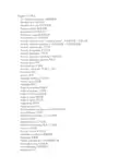
MWS NEMA IEC FEDERAL THERMAL INSULATION TYPE PRODUCT STANDARD STANDARD SPECIFICATION CLASS CODE (MW1000) (60317) (JW 1177)1os0c Plain Enamel PE NONE NONE NONE Formvar* F MW 15 (RD) MW 18 (SQ & RECT) 60317-1(RD) 60317-17(SQ & RECT) JW 1177/ 14 (RD) JW1177/ 16 (SQ & RECT) Formvar Bondable FB MW19 60317-5 JW 1177/613o•c Polyurethane Nylon Bondable -130 PE NONE NONE NONE1ss0c Polyurethane -155* P155 MW79 60317-20 JW1177/41 Polyurethane Nylon -155* PN155 MWB0 60317-21 JW1177/42Polyurethane Bondable -155* PB155 MW131 60317-35 NONEPolyurethane Nylon Bondable -155 PNB155 MW 136 NONE NONEDacron Glass -155 DGLAS 155 MW 45 (RD) MW 46 (SQ & RECT) NONE(RD) 60317-60(SQ & RECT) JW 1177/ 20 (RD) JW1177/ 25 (SQ & RECT) 1so·c Polyurethane -180• P180 MW82 60317-51 NONE Polyurethane Nylon -180* PN180 MW83 60317-55 NONEPolyester-imide• PT MW30 60317-8 JW 1177/ 12Polyester-Nylon* PTN MW76 60317-22 JW 1177/38Solderable Polyester* SPT MW77 60317-23 JW 1177/39Solderable Polyester Nylon• SPTN MW78 NONE JW 1177/ 40Polyurethane Bondable -180 PB180 MW132 NONE NONEPolyurethane Nylon Bondable -180 PNB180 MW137 NONE NONEPolyester-imide Bondable PTB NONE 60317-37 NONEPolyester-amide-imide Bondable* APTB MW 102 60317-38 NONESolderable Polyester Bondable SPTB NONE 60317-36 NONEDacron Glass High Temp DGLAS HT MW 51 (RD) MW 53 (SQ & RECT) NONE(RD) 60317-61(SQ & RECT) JW 1177/ 32 (RD) JW1177/ 34 (SQ & RECT) 200"C Polyester -200• PT200 MW74 60317-42 JW 1177/43 Polyester A/I Topcoat" APT MW 35 (RD) MW 36 (SQ & RECT) 60317-13(RD) 60317-29(SQ & RECT) JW 1177/ 14 (RD) JW1177/ 13 (SQ & RECT) Polyester A/I Polyamideimide• APT G MW73 60317-13 NONEPolyimide -ML* ML** MW 16 (RD) MW 20 (SQ & RECT) 60317-46(RD) 60317-47(SQ & RECT) JW 1177115 (RD) JW1177/ 18 (SQ & RECT)• UL Recognized Insulations•• Registered trademark of 1ST Industrial Summit Technology2 MWS Wire Industries, 31200 Cedar Valley Drive, Westlake Village, CA 91362 • Phone: 818-991-8553 • Fax: 818-706-0911 • Print Revision May 2016THERMAL INSULATIONGENERALCLASS APPLICATIONS1os•cPickup coils for guitars and other instruments CHARACTERISTICSPlain Enamel was one of the earliest film insulations developed for automotive ignition coils. Today it is primarily used in musical instruments for pickup coils. It is manufactured to single build dimensions and stocked in sizes 41 to 44 gaugeFormvar was an early synthetic insulation composed of modified polyvinyl resins designed for continuous operation at 105C. It has excellent Oil filled transformers, motors, solenoids,abrasion resistance and is compatible with m ost varnishes and impregnating compounds.superconducting coils or other cryogenic applications Formvar with a superimposed thermoplastic film for use in heat or solvent a ctivated self-b onding coils.Relays, yoke coils, self-supporting coils13o•c Class 130°C solderable polyurethane with superimposed thermoplastic polyvinyl b utyral film for heat or solvent activated self-bonding coils withVoice coils, yoke coils, self-supporting coilsexcellent bond strength at room temperature.1ss•cSolderable film composed of modified polyurethane resins designed mostly for fine wire applications with excellent resistance to moisture and Relays, high frequency coils and transformers, most solvents.solenoids, small motorsSolderable dual film c omposed of modified polyurethane resins with a polyamide (nylon) overcoat that provides improvement in severe winding Appliance motors, relays, torroidal coils, fractional HPoperations.motors Solderable polyurethane or polyurethane with nylon overcoat and a superimposed thermoplastic butyral film for coils requiring Class F service.Voice coils, helical coils, inductors, self-supporting coilsCoils may be bonded by heat or with denatured alcohol. Generally made as Type 1 i nsulation build equal to heavy overall diameter.Dacron Glass is a combination of glass and polyester fibers applied as a served filament over bare or film coated magnet wire and may be Dry transformers, Class B motorssupplied with an epoxy varnish or as fused unvarnished to prevent fraying of the fibers.1ao•cPolyurethane film designed for applications requiring high thermal resistance and low soldering temperature.Relays, ignition coils, solenoids, small transformers Polyurethane with polyamide (nylon) overcoat for applications requiring high thermal properties and chemical resistance.Relays, pulse transformers, small appliance motorsSoldering temperatures 430°C (14-23A WG) or 390°C (24AWG and finer). Film insulation composed of modified polyester resins with excellent chemical resistance.Solenoids, servo motors, small appliance motorsDual film composed of modified polyester resins with a nylon overcoat. Combines continuous 1 B0'C operating temperature and low coefficientMotor stators, fractional HP motorsof friction for superior winding and insertion properties.Film insulation composed of modified polyesterimide resins designed to solder at 470°C, generally made at 24 AWG and finer sizes. High temperature relays, transformers, automotive coilsDual film composed of modified polyesterimide resins with nylon overcoat for superior pertormance where winding stresses may be severe.Transformers, automotive coils, appliance motorsDesigned to solder at 470°C, this insulation is made mostly in heavier gauge sizes.One part (Polyurethane) or dual (Polyurethane Nylon) insulation system with superimposed thermoplastic film combining high thermal Self-supporting coils, relays, voice coilsresistance, solderability, and self-bonding features.These are wires that combine characteristics of various class 180°C film insulations with self-bonding feature. Bonding method depends on choice of bond coat. May be made as Type 1 (heavy diameter) or Type 2 (triple diameter) construction.Voice coils, inductors, yoke coils, small motorsLike Dacron G lass 155 e xcept t reated with high temperature organic v arnish. May be served over bare or film coated magnet wire. Large generators and alternators, dry type transformersAvailable only in shaped or heavy round wire sizes.200°COne part film system composed of THEIC modified polyester resins capable of continuous 200°C operating temperature designed Coils, relays, small transformers, small appliance motors specifically for finer size wires.A dual film insulation of polyester-amide-imide with polyamideimide (A/I) overcoat for superior windability, heat shock resistance, General purpose motors, fractional and integral motors solvent resistance, and overload protection.(hermetic and open), dry type transformers A triple f ilm s ystem composed of THEIC modified polyester, a corona resistant shield c oat, and polyamideimide (A/I) overcoat designed to Inverter duty motors, high voltage motorswithstand severe voltage stresses. Made as heavy build construction in round sizes 12 t hrough 24 A WG. Film composed of aromatic polyimide resin that features high cut through, exceptional chemical resistance, minimal outgassing and capableHigh temperature continuous duty coils, hermetically of continuous operation at 240°C in extremely harsh environments.sealed relays, fractional and integral HP motorsMWS Wire Industries, 31200 Cedar Valley Drive, Westlake Village, CA 91362 • Phone: 818-991-8553 • Fax: 818-706-0911 • 3Print Revision May 2016。
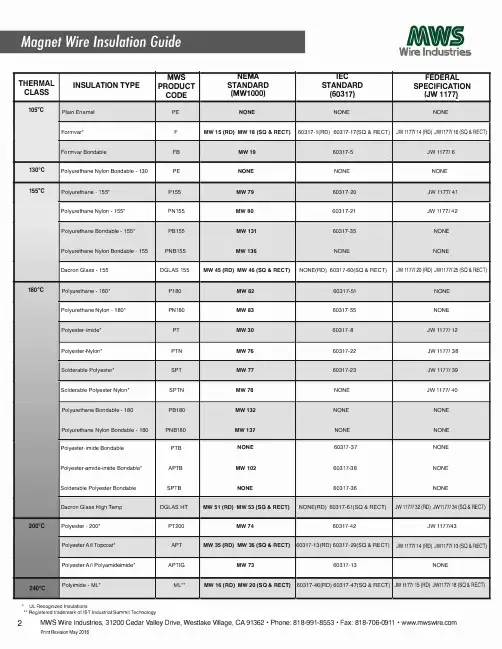
any loose powder particles.9.Procedure9.1Place the steel block on a sheet of preweighed or taredpaper.9.2Place the bushing on the block,on either side of thehole.9.3Fill the bushing slowly and carefully to three-quarters ofits height with powder.(A ring on the ID of the bushingindicates the proper fill height.)9.4With downward pressure on the bushing,slowly slidethe bushing toward the hole while twisting it.This gives asnowplow action to the powder as it falls slowly into the hole.Continue this motion until the bushing passes the hole.Stop,and again with downward pressure on the bushing,slide itstraight back over the hole to its starting position.The slidingaction must be slow enough to allow for complete filling of thesteel block cavity.9.5Remove the steel block from the preweighed paperbeing careful not to tip the block and spill additional powder onto the paper.9.6Transfer the preweighed or tared paper to a balance andweigh.Calculate the density from the following equation:Apparent Density,g/cm 35Mass in grams20cm 3(1)10.Report10.1Report the apparent density to the nearest 0.01g/cm 3.To minimize confusion with other test methods,report as Arnold Density,g/cm 3.11.Precision and Bias 11.1Precision —Precision has been determined from an interlaboratory study performed by Subcommittee B09.02.11.1.1Apparent Density Using the Arnold Meter :Repeatability r 50.08g/cm 3(2)11.1.2In 95%of such tests,on the basis of test error alone,duplicate tests in the same laboratory by the same operator,on one homogeneous lot of powder,will differ by no more than the stated amount.Reproducibility R 50.15g/m 3(3)11.1.3For 95%of comparative trials done in two different laboratories and on the basis of test error alone,a single test on the same homogeneous lot of powder will differ by no more than the stated amount.11.2Bias —No bias statement can be made because there is no accepted standard or reference powder for apparent density.12.Keywords12.1apparent density,Arnold Density,density of non-free-flowing powders,metalpowders FIG.1Arnold Apparent DensityMeterThe American Society for Testing and Materials takes no position respecting the validity of any patent rights asserted in connection with any item mentioned in this ers of this standard are expressly advised that determination of the validity of any such patent rights,and the risk of infringement of such rights,are entirely their own responsibility.This standard is subject to revision at any time by the responsible technical committee and must be reviewed everyfive years and if not revised,either reapproved or withdrawn.Your comments are invited either for revision of this standard or for additional standards and should be addressed to ASTM Headquarters.Your comments will receive careful consideration at a meeting of the responsible technical committee,which you may attend.If you feel that your comments have not received a fair hearing you should make your views known to the ASTM Committee on Standards,at the address shown below.This standard is copyrighted by ASTM,100Barr Harbor Drive,PO Box C700,West Conshohocken,PA19428-2959,United States. Individual reprints(single or multiple copies)of this standard may be obtained by contacting ASTM at the above address or at 610-832-9585(phone),610-832-9555(fax),or service@(e-mail);or through the ASTM website().。
德国科学家发明新型核工程防辐射屏蔽材
料
德国慕尼黑技术大学海因茨·迈尔-莱布尼茨试验中子源(又称慕尼黑实验反应堆2号FRMII)的研究人员发明一种可回收利用的新型防辐射屏蔽材料。
这种材料是一种粉末,含有铁颗粒、石蜡油和硼化合物,看起来像湿的黑色砂子。
与传统的表观密度大于等于每立方分米2.8公斤(2.8kgdm3)的重混凝土相比,重量要轻20%,但屏蔽效果相当。
与传统重混凝土相比,这种材料的最大优点是可重复使用:它填充在钢制容器中,置于实验终端以屏蔽辐射;若此处不再使用,可从容器中取出,异地再用。
这种材料目前已申请专利。
高精度电子比重计技术参数
产品描述:适用于微小塑料颗粒、高密度硬质合金、玻璃等样品的密度测试。
符合ASTM、JIS、GB/T、ISO、MPIF标准。
采用阿基米得原理浮力法,准确、直读量
测数值。
技术参数:
功能:
具有内藏砝码自动校正、开机自动校正、温差自动校正。
比重配件采取大水槽设计,降低吊栏线的浮力所造成的误差。
固体测试的最大尺寸(D100×W70×H25mm)
具有RS-232C计算机接口,可轻易的连接PC和打印机。
不吸水产品直接读出比重值:微小塑料颗粒、高密度硬质合金。
针对吸水产品:微小含油轴承含油率、孔隙率、生胚、烧结后密度的测试仪,提供演算软件,
配置
主机1套;
防腐蚀水槽1套;
比重配件组合1套;
其他机台附件。
售后服务
整机保修1年以上,终生维护,且响应时间在48小时以内;
相关耗材以8折以下折扣供应
1 / 1。
平面型电磁屏蔽材料镀金属层附着性能的测定1 范围本文件描述了平面型电磁屏蔽材料镀金属层附着性能的四种测定方法,包括试验条件、试验仪器和材料、试验样品、试验步骤、试验结果和试验报告。
本文件适用于表面具有镀金属层的平面型电磁屏蔽材料产品附着性能的质量控制。
2 规范性引用文件下列文件中的内容通过文中的规范性引用而构成本文件必不可少的条款。
其中,注日期的引用文件,仅该日期对应的版本适用于本文件;不注日期的引用文件,其最新版本(包括所有的修改单)适用于本文件。
GB/T 26667电磁屏蔽材料术语GB/T 2792—2014 胶粘带剥离强度的试验方法3 术语和定义GB/T 26667界定的以及下列术语和定义适用于本文件。
3.1平面型电磁屏蔽材料planar electromagnetic shielding material具有屏蔽电磁波干扰能力的平面型材料。
3.2被镀基材plated substrate在平面型电磁屏蔽材料(3.1)中承载镀金属层的材料。
3.3镀金属层附着性能 adhesion property of metallic coating镀金属层与被镀基材(3.2)表面之间的结合强度。
4 试验原理利用镀金属层和被镀基材之间的非同质性,在外力的作用下,观察镀金属层从被镀基材表面上脱落或被剥离的程度。
脱落或被剥离的原因是镀层与被镀基材结合力降低,脱落或被剥离程度越高则附着性能越差。
5 试验方法5.1 概述平面型电磁屏蔽材料镀金属层附着性能的测定可选用以下几种测试方法:摩擦剥离测试法、辊轮压力剥离测试法、划格测试法和弯折测试法。
5.2 摩擦剥离测试法5.2.1 试验条件试验环境温度(23±5)℃、相对湿度≤65%。
5.2.2 试验仪器和材料5.2.2.1 耐摩擦试验机耐摩擦试验机具有圆形摩擦表面的摩擦头,摩擦头直径为(16.0±0.1) mm,施加垂直向下的压力为(9.0±0.2) N,直线往复动程为(104±3) mm,往复频率为60 次/min。
a rXiv:074.1898v1[he p-th]15A pr27Electromagnetic Casimir densities for a wedge with a coaxial cylindrical shell A.A.Saharian ∗Department of Physics,Yerevan State University,1Alex Manoogian Street,375025Yerevan,Armenia February 1,2008Abstract Vacuum expectation values of the field square and the energy-momentum tensor for the electromagnetic field are investigated for the geometry of a wedge with a coaxal cylindrical boundary.All boundaries are assumed to be perfectly conducting and both regions inside and outside the shell are considered.By using the generalized Abel-Plana formula,the vacuum expectation values are presented in the form of the sum of two terms.The first one corresponds to the geometry of the wedge without the cylindrical shell and the second term is induced by the presence of the shell.The vacuum energy density induced by the shell is negative for the interior region and is positive for the exterior region.The asymptotic behavior of the vacuum expectation values are investigated in various limiting cases.It is shown that the vacuum forces acting on the wedge sides due to the presence of the cylindrical boundary are always attractive.PACS numbers:03.70.+k 1Introduction The Casimir effect is among the most interesting macroscopic manifestations of vacuum fluctu-ations.It have important implications on all scales,from cosmological to subnuclear,and has become in recent decades an increasingly popular topic in quantum field theory.In addition to its fundamental interest the Casimir effect also plays an important role in the fabrication and operation of nano-and micro-scale mechanical systems.The imposition of boundary conditions on a quantum field leads to the modification of the spectrum for the zero-point fluctuations and results in the shift in the vacuum expectation values for physical quantities such as the energy density and stresses.In particular,the confinement of quantum fluctuations causes forces that act on constraining boundaries.The particular features of the resulting vacuum forces depend on the nature of the quantum field,the type of spacetime manifold,the boundary geometries and the specific boundary conditions imposed on the field.Since the original work by Casimir [1]many theoretical and experimental works have been done on this problem (see,e.g.,[2,3,4,5]and references therein).Many different approaches have been used:mode summation methodwith combination of the zeta function regularization technique,Green function formalism,mul-tiple scattering expansions,heat-kernel series,etc.Advancedfield-theoretical methods have been developed for Casimir calculations during the past years[6,7,8].However,there are still difficulties in both interpretation and renormalization of the Casimir effect.Straightforward computations of geometry dependencies are conceptually complicated,since relevant informa-tion is subtly encoded in thefluctuations spectrum[8].Analytic solutions can usually be found only for highly symmetric geometries including planar,spherically and cylindrically symmetric boundaries.Recently the Casimir energy has been evaluated exactly for several less symmetric configurations of experimental interest.These include a sphere in front of a plane and a cylinder in front of a plane[9].A great deal of attention received the investigations of quantum effects for cylindrical bound-aries.In addition to traditional problems of quantum electrodynamics under the presence of material boundaries,the Casimir effect for cylindrical geometries can also be important to the flux tube models of confinement[10,11]and for determining the structure of the vacuum state in interactingfield theories[12].The calculation of the vacuum energy of electromagneticfield with boundary conditions defined on a cylinder turned out to be technically a more involved problem than the analogous one for a sphere.First the Casimir energy of an infinite perfectly conducting cylindrical shell has been calculated in Ref.[13]by introducing ultraviolet cutoffand later the corresponding result was derived by zeta function technique[14,15,16].The local characteristics of the corresponding electromagnetic vacuum such as energy density and vacuum stresses are considered in[17]for the interior and exterior regions of a conducting cylindrical shell,and in[18]for the region between two coaxial shells(see also[19]).The vacuum forces acting on the boundaries in the geometry of two cylinders are also considered in Refs.[20]. The scalar Casimir densities for a single and two coaxial cylindrical shells with Robin boundary conditions are investigated in Refs.[21,22].Less symmetric configuration of two eccentric per-fectly conducting cylinders is considered in Ref.[23].Vacuum energy for a perfectly conducting cylinder of elliptical section is evaluated in Ref.[24]by the mode summation method,using the ellipticity as a perturbation parameter.The Casimir forces acting on two parallel plates inside a conducting cylindrical shell are investigated in Ref.[25].Aside from their own theoretical and experimental interest,the exactly solvable problems with this type of boundaries are useful for testing the validity of various approximations used to deal with more complicated geometries.From this point of view the wedge with a coaxial cylindrical boundary is an interesting system,since the geometry is nontrivial and it includes two dynamical parameters,radius of the cylindrical shell and opening angle of the wedge.This geometry is also interesting from the point of view of general analysis for surface divergences in the expectation values of local physical observables for boundaries with discontinuities.The nonsmoothness of the boundary generates additional contributions to the heat kernel coefficients (see,for instance,the discussion in[26,27,28]and references therein).The present paper is concerned with local analysis of the vacuum of the electromagneticfield constrained to satisfy perfectly conducting boundary conditions on boundary surfaces of a wedge with a coaxial cylin-drical ly,we will study the vacuum expectation values of thefield squares and the energy-momentum tensor for the electromagneticfield for both regions inside and outside the cylindrical shell.In addition to describing the physical structure of the quantumfield at a given point,the energy-momentum tensor acts as the source of gravity in the Einstein equa-tions.It therefore plays an important role in modelling a self-consistent dynamics involving the gravitationalfield.The vacuum expectation value of the square of the electricfield determines the electromagnetic force on a neutral polarizable particle.Some most relevant investigations to the present paper are contained in Refs.[2,29,30,31,32,33],where the geometry of a wedge without a cylindrical boundary is considered for a conformally coupled scalar and electromag-neticfields in a four dimensional spacetime.The total Casimir energy of a semi-circular infinite cylindrical shell with perfectly conducting walls is considered in[34]by using the zeta function technique.For a scalarfield with an arbitrary curvature coupling parameter the Wightman function,the vacuum expectation values of thefield square and the energy-momentum tensor in the geometry of a wedge with an arbitrary opening angle and with a cylindrical boundary are evaluated in[35,36].Note that,unlike the case of conformally coupledfields,for a general coupling the vacuum energy-momentum tensor is angle-dependent and diverges on the wedge sides.Our method here employs the mode summation and is based on a variant of the gen-eralized Abel-Plana formula[37](see also Refs.[19,38]).This enables us to extract from the vacuum expectation values the parts due to a wedge without the cylindrical shell and to present the parts induced by the shell in terms of strongly convergent integrals.Note that the closely related problem of the vacuum densities induced by a cylindrical boundary in the geometry of a cosmic string is investigated in Refs.[39,40]for both scalar and electromagneticfields.We have organized the paper as follows.In the next section we describe the structure of the modes for a wedge with a cylindrical shell in the region inside the shell.By applying to the corresponding mode sums the generalized Abel-Plana formula,we evaluate the vacuum expectation values of the electric and magneticfield square.Various limiting cases of the general formulae are discussed.Section3is devoted to the investigation of the vacuum expectation values for the energy-momentum tensor of the electromagneticfield in the region inside the shell.The additional vacuum forces acting on the wedge sides due to the presence of the cylindrical boundary are evaluated.In section4we consider the vacuum densities for a wedge with the cylindrical shell in the exterior region with respect to the shell.Formulae for the shell contributions are derived and the corresponding surface divergences are investigated.The vacuum forces acting on the wedge sides are discussed.The main results are summarized and discussed in section5.2Vacuum expectation values of thefield square inside a cylin-drical shellConsider a wedge with the opening angleφ0and with a coaxial cylindrical boundary of radius a(seefigure1)assuming that all boundaries are perfectly conducting.In accordance with the problem symmetry,in the discussion below the cylindrical coordinates(r,φ,z)will be used.We are interested in the vacuum expectation values(VEVs)of thefield square and the energy-momentum tensor for the electromagneticfield.Expanding thefield operator in terms of the creation and annihilation operators and using the commutation relations,the VEV for a quantity F{A i,A k}bilinear in thefield can be presented in the form of the mode-sum0|F{A i,A k}|0 = αF{Aαi,A∗αk},(1)where{Aαi,A∗αk}is a complete set of solutions of the classicalfield equations satisfying the boundary conditions on the bounding surfaces and specified by a set of quantum numbersα.In accordance with formula(1),for the evaluation of the VEVs for the square of the electric and magneticfields and the energy-momentum tensor,the corresponding eigenfunctions are needed.In this section we consider the region inside the cylindrical shell(region I infigure 1).For the geometry under consideration there are two different types of the eigenfunctions corresponding to the transverse magnetic(TM)and transverse electric(TE)waves.In the discussion below we will specify these modes by the indexλ=0andλ=1for the TM and TE waves respectively.In the Coulomb gauge,the vector potentials for the TM and TE modes areδαα′,(4)ωwhere the integration goes over the region inside the shell.From this condition,by using the standard integral involving the square of the Bessel function,onefinds4qT qm(γa)β2α=ascending order.Consequently,the eigenfunctions are specified by the set of quantum numbers α=(k,m,λ,n ).First we consider the VEVs of the squares of the electric and magnetic fields inside the shell.Substituting the eigenfunctions(2)intothecorrespondingmode-sum formula,we find0|F 2|0 =4q2∞0dx f (x )+πJ (λ)qm (z )−1I (λ)qm (x ) e −qmπi f (e πi/2x )+e qmπi f (e −πi/2x ) ,(12)where Y ν(z )is the Neumann function and I ν(z ),K ν(z )are the modified Bessel functions.As it can be seen,for points away from the shell the contribution to the VEVs coming from the second integral term on the right-hand side of (12)is finite in the limit µ→0and,hence,the cutofffunction in this term can be safely removed.As a result the VEVs can be written in the form 0|F 2|0 = 0w |F 2|0w + F 2cyl ,(13)where0w |F 2|0w =qγ2 J ′2qm (γr )+q 2m 2γ2r 2 J 2qm (γr ) ,(14)and F 2 cyl =8q I (λ)qm (xa )G (ηF λ)[k,Φ(λ)qm (φ),I qm (xr )]x 2−k 2.(15)In formula Eq.(15)we have introduced the notationsG (0)[k,Φ(φ),f (x )]=(k 2r 2/x 2) Φ2(φ)f ′2(x )+Φ′2(φ)f 2(x )/x 2 +Φ2(φ)f 2(x ),(16)G (1)[k,Φ(φ),f (x )]=(k 2r 2/x 2−1)Φ2(φ)f ′2(x )+Φ′2(φ)f 2(x )/x 2 .(17)The second term on the right-hand side of Eq.(13)vanishes in the limit a →∞and the first one does not depend on a .Thus,we can conclude that the term 0w|F 2|0w corresponds to the part in the VEVs when the cylindrical shell is absent with the corresponding vacuum state |0w .Hence,the application of the generalized Abel-Plana formula enables us to extract from the VEVs the parts induced by the cylindrical shell without specifying the cutofffunction.In addition,these parts are presented in terms of the exponentially convergent integrals.First,let us concentrate on the part corresponding to the wedge without a cylindrical shell.First of all we note that in Eq.(14)the part which does not depend on the angular coordinate φis the same as in the corresponding problem of the cosmic string geometry with the angle deficit 2π−φ0(see Ref.[40]),which we will denote by 0s |F 2|0s .For this part we have0s |F 2|0s =qγ2 J ′2qm (γr )+q 2m2180πr 4,(18)where 0M|F 2|0Mis the part corresponding to the Minkowskian spacetime without boundaries and in the last expression we have removed the cutoff.To evaluate the part in (14)whichdepends on φ,we firstly consider the case when the parameter q is an integer.In this case the summation over m can be done by using the formula [41,42]∞ ′m =0cos(2qmφ)J 2qm (y )=1y 2 J 2qm (y ) =−1Substituting this in formula(14),the integrals remained are evaluated by introducing polar coordinates in the(k,γ)-plane.In this way onefinds0w|F2|0w = 0s|F2|0s −3(−1)ηF1180πr4−(−1)ηF1q22sin2(qφ)+1−q2 ,(23)withηE1=1andηB1=0.Though we have derived this formula for integer values of theparameter q,by the analytic continuation it is valid for non-integer values of this parameter aswell.The expression on the right of formula(23)is invariant under the replacementφ→φ0−φand,as we could expect,the VEVs are symmetric with respect to the half-planeφ=φ0/2.Formula(23)for F=E was derived in Ref.[32]within the framework of Schwinger’s sourcetheory.For q=1from formula(23)as a special case we obtain the renormalized VEVs of thefield square for a conducting plate.In this case x=r sinφis the distance from the plate andone hasF2 pl,ren=−3(−1)ηF1180x40−(−1)ηF1π32sin2(πx/x0)−1.(25)Now,we turn to the investigation of the parts in the VEVs of thefield square induced by the cylindrical boundary and given by formula(15).By using the formula∞dk k m ∞k dx xf(x)x2−k2=√2 2+1 ∞0dx x m+1f(x),(26) these parts are presented in the formF2 cyl=2qI(λ)qm(xa)G(ηFλ)[Φ(λ)qm(φ),I qm(xr)].(27) Here,for given functions f(x)andΦ(φ),we have introduced the notationsG(0)[Φ(φ),f(x)]=Φ2(φ)f′2(x)+Φ′2(φ)f2(x)/x2+2Φ2(φ)f2(x),(28)G(1)[Φ(φ),f(x)]=−Φ2(φ)f′2(x)−Φ′2(φ)f2(x)/x2.(29) As we see the parts in the VEVs induced by the cylindrical shell are symmetric with respect to the half-planeφ=φ0/2.The expression in the right-hand side of(27)isfinite for0<r<a including the points on the wedge sides,and diverges on the shell.Tofind the leading term in the corresponding asymptotic expansion,we note that near the shell the main contribution comes from large values of m.By using the uniform asymptotic expansions of the modified Bessel functions(see,for instance,[43]) for large values of the order,up to the leading order,for the points a−r≪a|sinφ|,a|sin(φ0−φ)| wefindF2 cyl≈−3(−1)ηF1πa4 r I1(x).(31) In this case the quantity B2 cyl takes afinite limiting value on the edge r=0,whereas E2 cyl vanishes as r2.For q<1+ηF1the main contribution comes form the mode with m=1and the shell-induced parts diverge on the edge r=0.The leading terms are given by the formulaF2 cyl≈−(−1)ηF1q(r/a)2(q−1)Iq(x)−K′q(x)3Vacuum energy-momentum tensor inside the cylindrical shell Now let us consider the VEV of the energy-momentum tensor in the region inside the cylindrical shell.Substituting the eigenfunctions(2)intothecorresponding mode-sum formula,for the non-zero components we obtain (no summation over i )0|T i i |0 =q4π2a∂2π2∞ ′m =0 λ=0,1 ∞0dxx 3K (λ)qm (xa )4π2∂I (λ)qm (xa )I 2qm (xr ),(39)with the notations F (i )[Φ(φ),f (y )]=Φ2(φ)f 2(y ),i =0,3,(40)F (i )[Φ(φ),f (y )]=−(−1)i Φ2(φ)f ′2(y )− Φ2(φ)−(−1)i Φ′2(φ)/y2 f 2(y ),i =1,2.(41)The diagonal components are symmetric with respect to the half-plane φ=φ0/2,whereas the off-diagonal component is an odd function under the replacement φ→φ0−φ.As it can be easily checked,the tensor T k i cyl is traceless and satisfies the covariant continuity equation ∇k T k i cyl =0.For the geometry under consideration the latter leads to the relations∂∂φT 22 cyl =0,(42)∂∂φ T 21 cyl = T 22 cyl .(43)As it is seen from formula(39),the off-diagonal component T12 cyl vanishes at the wedge sides and for these points the VEV of the energy-momentum tensor is diagonal.By using the in-equalities I′ν(x)< 1+ν2/x2Kν(x)for the modified Bessel functions,it can be seen that K′ν(x)/I′ν(x)+Kν(x)/Iν(x)<0.From this relation it follows that the vacuum energy density induced by the cylindrical shell in the interior region is always negative.The renormalized VEV of the energy-momentum tensor for the geometry without the cylin-drical shell is obtained by using the corresponding formulae for thefield square.For the corre-sponding energy density onefindsT00 w,ren=1720π2r4.(44) As we see the parts in the VEVs of thefield square which diverge on the wedge sides cancel out and the corresponding energy density isfinite everywhere except the edge.Formula(44) coincides with the corresponding result for the geometry of the cosmic string(see[44,45])with the angle deficit2π−φ0and in the corresponding formula q=2π/φ0.Other components are found from the tracelessness condition and the continuity equation and one has[29,30](see also [2])T k i w,ren=−(q2−1)(q2+11)240π2r4,(47) is the normal force acting per unit surface of the wedge for the case without a cylindrical boundary and the additional termp2cyl=− T22 cyl|φ=0,φ0=−qI(λ)qm(xa)F(λ)qm[I qm(xr)],(48)with the notationF(λ)ν[f(y)]= ν2f2(y)/y2,λ=0−f′2(y)−f2(y),λ=1,(49)is induced by the cylindrical shell.From formula(47)we see that the corresponding vacuum forces are attractive for q>1and repulsive for q<1.In particular,the equilibrium position corresponding to the geometry of a single plate(q=1)is unstable.As regards to the part induced by the cylindrical shell,from(48)it follows that p2cyl<0and,hence,the corresponding forces are always attractive.Now,let us discuss the behavior of the boundary-induced part in the VEV of the energy-momentum tensor in the asymptotic region of the parameters.Near the cylindrical shell the main contribution comes from large values of m.Thus,using the uniform asymptotic expansionsfor the modified Bessel functions for large values of the order,up to the leading order,for the points a −r ≪a |sin φ|,a |sin(φ0−φ)|we findT 00 cyl ≈−160π2a , T 11 cyl ≈(a −r )−24π2a 4 ∞0dx x 3K ′0(x )a 4,i =0,3.(51)For the components (no summation over i ) T i i cyl ,i =1,2,when q >1the main contributionagain comes form m =0term and one has T i i cyl ≈− T 00 cyl ,i =1,2.For q <1the main contribution into the components T i i cyl ,i =1,2,comes from the term m =1and we have (nosummation over i )T i i cyl ≈(−1)i q cos(2qφ)a 2(q −1) ∞0dx x 2q +1 K q (x )I ′q(x ) ,i =1,2.(52)In this case the radial and azimuthal stresses induced by the cylindrical shell diverge on the edge r =0.In the case q =1the sum of the contributions of the terms with m =0and m =1given by formulae(51)and (52)should be taken.For the off-diagonal component the main contribution comes from the m =1mode with the leading termT 12 cyl ≈q sin(2qφ)a 2q −1 ∞0dx x 2q +1 K q (x )I ′q(x ) ,(53)and this component vanishes on the edge for q >1/2.In the limit q ≫1,the contribution of the modes with m 1is suppressed by the factor exp[−2qm ln(a/r )]and the main contribution comes from the m =0mode.The leading terms are given by the formulae (no summation over i )T i i cyl ≈q I ′0(x )I 20(xr/a ),i =0,3,(54)T i i cyl ≈−qI ′0(x ) I 20(xr/a )+(−1)i I 21(xr/a ),i =1,2.(55)Though in this limit the vacuum densities are large,due to the factor 1/q in the spatial volume,the corresponding global quantities tend to finite value.In particular,as it follows from Eq.(55),in the limit under consideration one has T i i cyl >0.Note that in the same limit the parts corresponding to the wedge without the cylindrical shell behave as q 4and,hence,for points not too close to the shell these parts dominate in the VEVs.In figures 2-5we have plotted the parts in the VEVs of the energy-momentum tensor induced by the cylindrical shell,a 4 T k i cyl ,as functions of x =(r/a )cos φand y =(r/a )sin φ,for a wedge with the opening angle φ0=π/2.In figure 6we have presented the dependence of the effective azimuthal pressure induced by the cylindrical shell on the wedge sides,a 4p 2cyl ,as a function of r/a for different values of the parameter q .--0a 4<T 00>cylFigure 2:The part in the VEV of the energy density,a 4 T 00 cyl,induced by the cylindrical boundary as a function on x =(r/a )cos φand y =(r/a )sin φfor a wedge with φ0=π/2.-0.6a 4<T 11>cyl Figure 3:The part in the VEV of the radial stress,a 4 T 11 cyl,induced by the cylindrical boundary as a function on x =(r/a )cos φand y =(r/a )sin φfor a wedge with φ0=π/2.a4<T22>cylFigure4:The part in the VEV of the azimuthal stress,a4 T22 cyl,induced by the cylindrical boundary as a function on x=(r/a)cosφand y=(r/a)sinφfor a wedge withφ0=π/2.a3<T21>cyl-Figure5:The part in the VEV of the off-diagonal component,a4 T21 cyl,induced by the cylin-drical boundary as a function on x=(r/a)cosφand y=(r/a)sinφfor a wedge withφ0=π/2.0.10.20.30.40.5r a 0.8 0.60.4 0.2a 4p 2 c y l 0.513Figure 6:The effective azimuthal pressure induced by the cylindrical shell on the wedge sides,a 4p 2cyl ,as a function of r/a .The numbers near the curves correspond to the values of the parameter q .There are several special cases of interest for the geometry of boundaries we have consid-ered.The case φ0=πcorresponds to the semi-circular cylinder.The Casimir energy for the corresponding interior region is evaluated in Ref.[34]by using the zeta function technique.The case φ0=2πcorresponds to the geometry of a cylindrical shell with a coaxial half-plane.And finally,the limit φ0→0,r,a →∞,assuming that a −r and aφ0≡b are fixed,corresponds to the geometry of two parallel plates separated by a distance b ,perpendicularly intersected by the third plate.In the latter case it is convenient to introduce rectangular coordinates (x ′1,x ′2,x ′3)=(x,y,z )with the relations x =a −r ,y =rφ.The components of the tensors in these coordinates we will denote by primes.The corresponding vacuum energy-momentum tensor is presented in the form0|T ′i k |0 = T ′i k (0)+ T ′i k (1),(56)where T ′i k (0)is the vacuum expectation value in the region between two parallel plates located at y =0and y =a and T ′i k (1)is induced by the intersecting plate at x =0.The latter is related to the quantities investigated above by formulaeT ′i i (1)=lim T i i cyl , T ′12 (1)=−lim 1for the vector potential are obtained from formulae (2)bythereplacement J qm (γr )→g (λ)qm (γa,γr )=J qm (γr )Y (λ)qm (γa )−Y qm (γr )J (λ)qm (γa ),(58)where,as before,λ=0,1correspond to the waves of the electric and magnetic types,respec-tively.Now,the eigenvalues for γare continuous and in the normalization condition (4)the corresponding part on the right is presented by the delta function.As the normalization inte-gral diverges for γ′=γ,the main contribution into the integral comes from large values of r and we can replace the cylindrical functions with the argument γr by their asymptotic expressions for large values of the argument.By this way it can be seen that the normalization coefficient in the exterior region is determined by the relationβ−2α=8ππ∞ ′m =0 +∞−∞dk ∞0dγ λ=0,1γ3k 2+γ2g (ηF λ)[Φ(λ)qm (φ),g (λ)qm (γa,γr )]J (λ)2qm (γa )+Y (λ)2qm (γa )=g (ηF λ)[Φ(λ)qm (φ),J qm (γr )]−1H (s )(λ)qm (γa )g (ηF λ)[Φ(λ)qm (φ),H (s )qm (γr )],(61)where H (1,2)qm (z )are the Hankel functions.In order to transform the integral over γwith the last term on the right of (61),in the complex plane γwe rotate the integration contour by the angle π/2for the term with s =1and by the angle −π/2for the term with s =2.Due to the well-known properties of the Hankel functions the integrals over the corresponding parts of the circles of large radius in the upper and lower half-planes vanish.After introducing the modified Bessel functions and integrating over k with the help of formula (26),we can write the VEVs of the field square in the form (13),where the part induced by the cylindrical shell is given by the formulaF 2 cyl =2q K (λ)qm (xa )G (ηF λ)[Φ(λ)qm (φ),K qm (xr )].(62)In this formula the functions G (ηF λ)[Φ(φ),f (x )]are defined by formulae (28),(29).Comparing this result with formula (27),we see that the expressions for the shell-induced parts in the interior and exterior regions are related by the interchange I qm ⇄K qm .The VEV (62)diverges on the cylindrical shell with the leading term being the same as that for the interior region.At large distances from the cylindrical shell we introduce a new integration variable y =xr andexpand the integrand over a/r .For q >1the main contribution comes from the lowest mode m =0and up to the leading order we haveE 2 cyl ≈4q r 2, B 2 cyl ≈−28q r2.(63)For q <1the dominant contribution into the VEVs at large distances is due to the mode m =1with the leading termF 2 cyl ≈−4q 2(q +1)r 2q cos(2qφ)2q +1.(64)For the case q =1the contributions of the modes m =0and m =1are of the same order and the corresponding leading terms are obtained by summing these contributions.The latter are given by the right-hand sides of formulae (63)and (64).As we see,at large distances the part induced by the cylindrical shell is suppressed with respect to the part corresponding to the wedge without the shell by the factor (a/r )2βwith β=min(1,q ).Now we turn to the VEVs of the energy-momentum tensor in the exterior region.Substi-tuting the eigenfunctions into the corresponding mode-sum formula,one finds (no summation over i )0|T i i |0 =q J (λ)2qm (γa )+Y (λ)2qm (γa ),(65) 0|T 12|0 =−q∂r ∞ ′m =0m sin(2qmφ)+∞−∞dk ∞0dγ λ=0,1(−1)λγg (λ)2qm (γa,γr )k 2+γ2.(66)Subtracting from these VEVs the corresponding expression for the wedge without the cylindrical boundary,analogously to the case of the field square,it can be seen that the VEVs are presented in the form (37),with the parts induced by the cylindrical shell given by the formulae (no summation over i )T i i cyl =q K (λ)qm (xa )F (i )[Φ(λ)qm (φ),K qm (xr )],(67) T 12 cyl =q 2∂r ∞ ′m =0m sin(2qmφ) λ=0,1(−1)λ ∞0dxx I (λ)qm (xa )π2∞ ′m =0 λ=0,1 ∞0dxx 3I (λ)qm (xa )The leading divergence in the boundary induced part(67)on the cylindrical surface is given by the same formulae as for the interior region.For large distances from the shell and for q >1the main contribution into the VEVs of the diagonal components comes from the m =0,λ=1term and one has (no summation over i )T i i cyl ≈−qc ir 2,c 0=c 3=2,c 1=1,c 2=−5.(70)In the case q <1the main contribution into the VEVs of the diagonal components at large distances from the cylindrical shell comes from the m =1mode.The leading terms in the corresponding asymptotic expansions are given by the formulaeT i i cyl≈−q 2(q +1)c i (q )cos(2qφ)r 2q ,(71)with the notationsc 0(q )=c 3(q )=1(2q +1)(2q +3),c 2(q )=−q +12q +1sin(2qφ)r 2q .(73)For large values of q ,q ≫1,the contribution of the terms with m >0is suppressed by the factor exp[−2qm ln(r/a )]and the main contribution comes form the m =0term with the behavior F 2 cyl ∝q and T k i cyl ∝q .In figure 7we have plotted the dependence of the effective azimuthal pressure induced by the cylindrical shell on the wedge sides,a 4p 2cyl ,as a function of r/a for q =1.1.4 1.5 1.6 1.7 1.8 1.92r a 0.80.60.4 0.2a 4p 2 c y l Figure 7:The effective azimuthal pressure induced by the cylindrical shell on the wedge sides,a 4p 2cyl ,as a function of r/a in the exterior region for q =1.The curves for the values q =0.5,3are close to the plotted one.。