A Texture-Based Hardware-Independent Technique for Time-Varying Volume Flow Visualization

计算机行业常见设备名称英语词汇汇总下面是计算机行业常见设备名称，大家可以参考下。

ATAPI(AT Attachment Packet Interface)BCF(Boot Catalog File，启动目录文件)BIF(Boot Image File，启动映像文件)CDR(CD Recordable，可记录光盘)CD-ROM/XA(CD-ROM eXtended Architecture，唯读光盘增强形架构)CDRW(CD-Rewritable，可重复刻录光盘)CLV(Constant Linear Velocity，恒定线速度)DAE(digital Audio Extraction，数据音频抓取)DDSS(Double Dynamic Suspension System，双悬浮动态减震系统)DDSS II(Double Dynamic Suspension System II，第二代双层动力悬吊系统)PCAV(Part Constant Angular Velocity，部分恒定角速度)VCD(Video CD，视频CD)AAS(Automatic Area Seagment?)dpi(dot per inch，每英寸的打印像素)ECP(Extended Capabilities Port，延长能力端口)EPP(Enhanced Parallel Port，增强形平行接口)IPP(Inter Printing Protocol，因特网打印协议)ppm(paper per minute，页/分)SPP(Standard Parallel Port，标准并行口)TET(Text Enhanced Technology，文本增强技术)USBDCDPD(Universal Serial Bus Device Class Definition for Printing Devices，打印设备的通用串行总线级标准) VD(Variable Dot，变点式列印)TWAIN(Toolkit Without An Interesting Name)协议AAT(Average aess time，平均存取时间)ABS(Auto Balance System，自动平衡系统)ASMO(Advanced Storage Mago-Optical，增强形光学存储器) AST(Average Seek time，平均寻道时间)ATA(AT Attachment，AT扩展型)ATOMM(Advanced super Thin-layer and high-Output Metal Media，增强形超薄高速金属媒体)bps(bit per second，位/秒)CAM(Common Aess Model，公共存取模型)CSS(Common Command Set，通用指令集)DMA(Direct Memory Aess，直接内存存取)DVD(Digital Video Disk，数字视频光盘)EIDE(enhanced Integrated Drive Electronics，增强形电子集成驱动器)FAT(File Allocation Tables，文件分配表)FDBM(Fluid dynamic bearing motors，液态轴承马达)FDC(Floppy Disk Controller，软盘驱动器控制装置)FDD(Floppy Disk Driver，软盘驱动器)GMR(giant magoresistive，巨型磁阻)HDA(head disk assembly，磁头集合)HiFD(high-capacity floppy disk，高容量软盘)IDE(Integrated Drive Electronics，电子集成驱动器)LBA(Logical Block Addressing，逻辑块寻址)MBR(Master Boot Record，主引导记录)MTBF(Mean Time Before Failure，平均故障时间)PIO(Programmed Input Output，可编程输入输出模式)PRML(Partial Response Maximum Likelihood，最大可能部分反响，用于提高磁盘读写传输率)RPM(Rotation Per Minute，转/分)RSD：(Removable Storage Device移动式存储设备)SCSI(Small Computer System Interface，小型计算机系统接口)SCMA：(SCSI Configured Auto Magically，SCSI自动配置)S.M.A.R.T.(Self-Monitoring， Analysis and Reporting Technology，自动监测、分析和报告技术)SPS(Shock Protection System，抗震保护系统)STA(SCSI Trade Association，SCSI同业公会)Ultra DMA(Ultra Direct Memory Aess，超高速直接内存存取) LVD(Low Voltage Differential)Seagate硬盘技术DiscWizard(磁盘控制软件)DST(Drive Self Test，磁盘自检程序)SeaShield(防静电防撞击外壳)3DPA(3D Positional Audio，3D定位音频)AC(Audio Codec，音频多媒体数字信号编解码器)Auxiliary Input(辅助输入接口)CS(Channel Separation，声道别离)DS3D(DirectSound 3D Streams)DSD(Direct Stream Digital，直接数字信号流)DSL(Down Loadable Sample，可下载的取样音色)DLS-2(Downloadable Sounds Level 2，第二代可下载音色)EAX(Environmental Audio Extensions，环境音效扩展技术) Extended Stereo(扩展式立体声)FM(Frequency Modulation，频率调制)FIR(finite impulse response，有限推进响应)FR(Frequence Response，频率响应)FSE(Frequency Shifter Effect，频率转换效果)HRTF(Head Related Transfer Function，头部关联传输功能) IID(Interaural Intensity Difference，两侧声音强度差异) IIR(infinite impulse response，无限推进响应)Interactive Around-Sound(交互式环绕声)Interactive 3D Audio(交互式3D音效)ITD(Interaural Time Difference，两侧声音时间延迟差异) MIDI：( Musical Instrument Digital Interface乐器数字接口)NDA：( non-DWORD-aligned ，非DWORD排列)Raw PCM：( Raw Pulse Code Modulated元脉码调制)RMA：( RealMedia Architecture实媒体架构)RTSP： (Real Time Streaming Protocol实时流协议)SACD(Super Audio CD，超级音乐CD)SNR(Signal to Noise Ratio，信噪比)S/PDIF(Sony/Phillips Digital Interface，索尼/飞利普数字接口)SRS： (Sound Retrieval System声音修复系统)Surround Sound(环绕立体声)Super Intelligent Sound ASIC(超级智能音频集成电路)THD+N(Total Harmonic Distortion plus Noise，总谐波失真加噪音)QEM(Qsound Environmental Modeling，Qsound环境建模扬声器组)WG(Wave Guide，波导合成)WT(Wave Table，波表合成)3D：(Three Dimensional，三维)3DS(3D SubSystem，三维子系统)AE(Atmospheric Effects，雾化效果)AFR(Alternate Frame Rendering，交替渲染技术)Anisotropic Filtering(各向异性过滤)APPE(Advanced Packet Parsing Engine，增强形帧解析引擎) AV(Analog Video，模拟视频)Back Buffer，后置缓冲Backface culling(隐面消除)Battle for Eyeballs(眼球大战，各3D图形芯片公司为了争夺用户而作的竞争)Bilinear Filtering(双线性过滤)CEM(cube environment mapping，立方环境映射)CG(Computer Graphics，计算机生成图像)Clipping(剪贴纹理)Clock Synthesizer，时钟合成器pressed textures(压缩纹理) Concurrent Command Engine，协作命令引擎Center Processing Unit Utilization，中央处理器占用率DAC(Digitalto Analog Converter，数模传换器)Decal(印花法，用于生成一些半透明效果，如：鲜血飞溅的场面)DFP(Digital Flat Panel，数字式平面显示器)DFS：( Dynamic Flat Shading动态平面描影，可用作加速Dithering抖动)Directional Light，方向性光源DME：( Direct Memory Execute直接内存执行)DOF(Depth of Field，多重境深)Double Buffering(双缓冲区)DIR(Direct Rendering Infrastructure，基层直接渲染)DVI(Digital Video Interface，数字视频接口)DxR：( DynamicXTended Resolution动态可扩展分辨率)DXTC(Direct X Texture Compress，DirectX纹理压缩，以S3TC为根底)Dynamic Z-buffering(动态Z轴缓冲区)，显示物体远近，可用作远景E-DDC(Enhanced Display Data Channel，增强形视频数据通道协议，定义了显示输出与主系统之间的通讯通道，能提高显示输出的画面质量)Edge Anti-aliasing，边缘抗锯齿失真E-EDID(Enhanced Extended Identification Data，增强形扩充身份辨识数据，定义了电脑通讯视频主系统的数据格式)Execute Buffers，执行缓冲区environment mapped bump mapping(环境凹凸映射)Extended Burst Transactions，增强式突发处理Front Buffer，前置缓冲Flat(平面描影)Frames rate is King(帧数为王)FSAA(Full Scene Anti-aliasing，全景抗锯齿)Fog(雾化效果)flip double buffered(反转双缓存)fog table quality(雾化表画质)GART(Graphic Address Remappng Table，图形地址重绘表) Gouraud Shading，高洛德描影，也称为内插法均匀涂色GPU(Graphics Processing Unit，图形处理器)GTF(Generalized Timing Formula，一般程序时间，定义了产生画面所需要的时间，包括了诸如画面刷新率等)HAL(Hardware Abstraction Layer，硬件抽像化层)hardware motion pensation(硬件运动补偿)HDTV(high definition television，高清晰度电视)HEL： Hardware Emulation Layer(硬件模拟层)high triangle count(复杂三角形计数)ICD(Installable Client Driver，可安装客户端驱动程序) IDCT(Inverse Discrete Cosine Transform，非连续反余弦变换，GeForce的DVD硬件强化技术)Immediate Mode，直接模式IPPR： (Image Processing and Pattern Recognition图像处理和模式识别)large textures(大型纹理)LF(Linear Filtering，线性过滤，即双线性过滤)lighting(光源)lightmap(光线映射)Local Peripheral Bus(局域边缘总线)mipmapping(MIP映射)Modulate(调制混合)Motion Compensation，动态补偿motion blur(模糊移动)MPPS：(Million Pixels Per Second，百万个像素/秒)Multi-Resolution Mesh，多重分辨率组合Multi Threaded Bus Master，多重主控Multitexture(多重纹理)nerest Mipmap(邻近MIP映射，又叫点采样技术)Overdraw(透支，全景渲染造成的浪费)partial texture downloads(并行纹理传输)Parallel Processing Perspective Engine(平行透视处理器) PC(Perspective Correction，透视纠正)PGC(Parallel Graphics Configuration，并行图像设置)pixel(Picture element，图像元素，又称P像素，屏幕上的像素点)point light(一般点光源)Precise Pixel Interpolation，准确像素插值Procedural textures(可编程纹理)RAMDAC(Random Aess Memory Digital to Analog Converter，随机存储器数/模转换器)Reflection mapping(反射贴图)ender(着色或渲染)S端子(Seperate)S3(Sight、Sound、Speed，视频、音频、速度)S3TC(S3 Texture Compress，S3纹理压缩，仅支持S3显卡)S3TL(S3 Transformation & Lighting，S3多边形转换和光源处理)Screen Buffer(屏幕缓冲)SDTV(Standard Definition Television，标准清晰度电视)SEM(spherical environment mapping，球形环境映射)Shading，描影Single Pass Multi-Texturing，单通道多纹理SLI(Scanline Interleave，扫描线间插，3Dfx的双Voodoo 2配合技术)Smart Filter(智能过滤)soft shadows(柔和阴影)soft reflections(柔和反射)spot light(小型点光源)SRA(Symmetric Rendering Architecture，对称渲染架构)Stencil Buffers(模板缓冲)Stream Processor(流线处理)SuperScaler Rendering，超标量渲染TBFB(Tile Based Frame Buffer，碎片纹理帧缓存)texel(T像素，纹理上的像素点)Texture Fidelity(纹理真实性)texture swapping(纹理交换)T&L(Transform and Lighting，多边形转换与光源处理)T-Buffer(T缓冲，3dfx Voodoo4的特效，包括全景反锯齿Full-scene Anti-Aliasing、动态模糊Motion Blur、焦点模糊Depth of Field Blur、柔和阴影Soft Shadows、柔和反射Soft Reflections)TCA(Twin Cache Architecture，双缓存构造)Transparency(透明状效果)Transformation(三角形转换)Trilinear Filtering(三线性过滤)Texture Modes，材质模式TMIPM： (Trilinear MIP Mapping 三次线性MIP材质贴图)UMA(Unified Memory Architecture，统一内存架构)Visualize Geometry Engine，可视化几何引擎Vertex Lighting(顶点光源)Vertical Interpolation(垂直调变)VIP(Video Interface Port，视频接口)ViRGE： (Video and Rendering Graphics Engine视频描写图形引擎)Voxel(Volume pixels，立体像素，Novalogic的技术)VQTC(Vector-Quantization Texture Compression，向量纹理压缩)VSIS(Video Signal Standard，视频信号标准)v-sync(同步刷新)Z Buffer(Z缓存)ASIC： (Application Specific Integrated Circuit特殊应用积体电路)ASC(Auto-Sizing and Centering，自动调效屏幕尺寸和中心位置)ASC(Anti Static Coatings，防静电涂层)AGAS(Anti Glare Anti Static Coatings，防强光、防静电涂层)BLA： (Bearn Landing Area电子束落区)BMC(Black Matrix Screen，超黑矩阵屏幕)CRC： (Cyclical Redundancy Check循环冗余检查)CRT(Cathode Ray Tube，阴极射线管)DDC：(Display Data Channel，显示数据通道 )DEC(Direct Etching Coatings，外表蚀刻涂层)DFL(Dynamic Focus Lens，动态聚焦)DFS(Digital Flex Scan，数字伸缩扫描)DIC： (Digital Image Control数字图像控制)Digital Multiscan II(数字式智能多频追踪)DLP(digital Light Processing，数字光处理)DOSD：(Digital On Screen Display同屏数字化显示)DPMS(Display Power Management Signalling，显示能源管理信号)Dot Pitch(点距)DQL(Dynamic Quadrapole Lens，动态四极镜)DSP(Digital Signal Processing，数字信号处理)EFEAL(Extended Field Elliptical Aperture Lens，可扩展扫描椭圆孔镜头)FRC：(Frame Rate Control帧比率控制)HVD(High Voltage Differential，高分差动)LCD(liquid crystal display，液晶显示屏)LCOS： (Liquid Crystal On Silicon硅上液晶)LED(light emitting diode，光学二级管)L-SAGIC(Low Power-Small Aperture G1 wiht Impregnated Cathode，低电压光圈阴极管)LVD(Low Voltage Differential，低分差动)LVDS：(Low Voltage Differential Signal低电压差动信号) MALS(Multi Astigmatism Lens System，多重散光聚焦系统) MDA(Monochrome Adapter，单色设备)MS： (Magic Sensors磁场感应器)Porous Tungsten(活性钨)RSDS： (Reduced Swing Differential Signal小幅度摆动差动信号)SC(Screen Coatings，屏幕涂层)Single Ended(单终结)Shadow Mask(阴罩式)TDT(Timeing Detection Table，数据测定表)TICRG： (Tungsten Impregnated Cathode Ray Gun钨传输阴级射线枪)TFT(thin film transistor，薄膜晶体管)UCC(Ultra Clear Coatings，超清晰涂层)VAGP：( Variable Aperature Grille Pitch可变间距光栅) VBI：( Vertical Blanking Interval垂直空白间隙)VDT(Video Display Terminals，视频显示终端)VRR： (Vertical Refresh Rate垂直扫描频率 )ADIMM(advanced Dual In-line Memory Modules，高级双重内嵌式内存模块)AMR(Audio/Modem Riser;音效/调制解调器主机板附加直立插卡) AHA(Aelerated Hub Architecture，加速中心架构)ASK IR(Amplitude Shift Keyed Infra-Red，长波形可移动输入红外线)ATX： AT Extend(扩展型AT)BIOS(Basic Input/Output System，根本输入/输出系统)CSE(Configuration Space Enable，可分配空间)DB：(Device Bay，设备插架 )DMI(Desktop Management Interface，桌面管理接口)EB(Expansion Bus，扩展总线)EISA(Enhanced Industry Standard Architecture，增强形工业标准架构)EMI(Electromagic Interference，电磁干扰)ESCD(Extended System Configuration Data，可扩展系统配置数据)FBC(Frame Buffer Cache，帧缓冲缓存)FireWire(火线，即IEEE1394标准)FSB： (Front Side Bus，前置总线，即外部总线 )FWH( Firmware Hub，固件中心)GMCH(Graphics & Memory Controller Hub，图形和内存控制中心)GPIs(General Purpose Inputs，普通操作输入)ICH(Input/Output Controller Hub，输入/输出控制中心)IR(infrared ray，红外线)IrDA(infrared ray，红外线通信接口可进展局域网存取和文件共享)ISA：(Industry Standard Architecture，工业标准架构 )ISA(instruction set architecture，工业设置架构)MDC(Mobile Daughter Card，移动式子卡)MRH-R(Memory Repeater Hub，内存数据处理中心)MRH-S(SDRAM Repeater Hub，SDRAM数据处理中心)MTH(Memory Transfer Hub，内存转换中心)NGIO(Next Generation Input/Output，新一代输入/输出标准) P64H(64-bit PCI Controller Hub，64位PCI控制中心)PCB(printed circuit board，印刷电路板)PCBA(Printed Circuit Board Assembly，印刷电路板装配)PCI：(Peripheral Component Interconnect，互连外围设备 ) PCI SIG(Peripheral Component Interconnect Special Interest Group，互连外围设备专业组)POST(Power On Self Test，加电自测试)RNG(Random number Generator，随机数字发生器)RTC： (Real Time Clock 实时时钟)KBC(KeyBroad Control，键盘控制器)SAP(Sideband Address Port，边带寻址端口)SBA(Side Band Addressing，边带寻址)SMA： (Share Memory Architecture，共享内存构造 )STD(Suspend To Disk，磁盘唤醒)STR(Suspend To RAM，内存唤醒)SVR： (Switching Voltage Regulator 交换式电压调节)USB(Universal Serial Bus，通用串行总线)USDM(Unified System Diagnostic Manager，统一系统监测管理器)VID(Voltage Identification Definition，电压识别认证)VRM (Voltage Regulator Module，电压调整模块)ZIF： (Zero Insertion Force，零插力 )主板技术Gigabyte ACOPS：(Automatic CPU OverHeat Prevention SystemCPU 过热预防系统)SIV： (System Information Viewer系统信息观察)磐英ESDJ(Easy Setting Dual Jumper，简化CPU双重跳线法) 浩鑫UPT(USB、PANEL、LINK、TV-OUT四重接口)芯片组ACPI(Advanced Configuration and PowerInterface，先进设置和电源管理)AGP(Aelerated Graphics Port，图形加速接口)I/O(Input/Output，输入/输出)MIOC： (Memory and I/O Bridge Controller，内存和I/O桥控制器)NBC： (North Bridge Chip北桥芯片)PIIX： (PCI ISA/IDE Aelerator加速器)PSE36： (Page Size Extension 36-bit，36位页面尺寸扩展模式 )PXB：(PCI Expander Bridge，PCI增强桥 )RCG： (RAS/CAS Generator，RAS/CAS发生器 )SBC： (South Bridge Chip南桥芯片)SMB： (System Management Bus全系统管理总线)SPD(Serial Presence Detect，内存内部序号检测装置)SSB： (Super South Bridge，超级南桥芯片 )TDP：(Triton Data Path数据路径)TSC： (Triton System Controller系统控制器)QPA： (Quad Port Aeleration四接口加速)3DNow!(3D no waiting)ALU(Arithmetic Logic Unit，算术逻辑单元)AGU(Address Generation Units，地址产成单元)BGA(Ball Grid Array，球状矩阵排列)BHT(branch prediction table，分支预测表)BPU(Branch Processing Unit，分支处理单元)Brach Pediction(分支预测)CMOS： (Complementary Metal Oxide Semiconductor，互补金属氧化物半导体 )CISC(Complex Instruction Set Computing，复杂指令集计算机)CLK(Clock Cycle，时钟周期)COB(Cache on board，板上集成缓存)COD(Cache on Die，芯片内集成缓存)CPGA(Ceramic Pin Grid Array，陶瓷针型栅格阵列)CPU(Center Processing Unit，中央处理器)Data Forwarding(数据前送)Decode(指令解码)DIB(Dual Independent Bus，双独立总线)EC(Embedded Controller，嵌入式控制器)Embedded Chips(嵌入式)EPIC(explicitly parallel instruction code，并行指令代码) FADD(Floationg Point Addition，浮点加)FCPGA(Flip Chip Pin Grid Array，反转芯片针脚栅格阵列)FDIV(Floationg Point Divide，浮点除)FEMMS：(Fast Entry/Exit Multimedia State，快速进入/退出多媒体状态)FFT(fast Fourier transform，快速热欧姆转换)FID(FID：Frequency identify，频率鉴别号码)FIFO(First Input First Output，先入先出队列)flip-chip(芯片反转)FLOP(Floating Point Operations Per Second，浮点操作/秒) FMUL(Floationg Point Multiplication，浮点乘)FPU(Float Point Unit，浮点运算单元)FSUB(Floationg Point Subtraction，浮点减)GVPP(Generic Visual Perception Processor，常规视觉处理器)HL-PBGA：外表黏著，高耐热、轻薄型塑胶球状矩阵封装IA(Intel Architecture，英特尔架构)ICU(Instruction Control Unit，指令控制单元)ID：(identify，鉴别号码 )IDF(Intel Developer Forum，英特尔开发者论坛)IEU(Integer Execution Units，整数执行单元)IMM：( Intel Mobile Module，英特尔移动模块 )Instructions Cache，指令缓存Instruction Coloring(指令分类)IPC(Instructions Per Clock Cycle，指令/时钟周期)ISA(instruction set architecture，指令集架构)KNI(Katmai New Instructions，Katmai新指令集，即SSE)Latency(潜伏期)LDT(Lightning Data Transport，闪电数据传输总线)Local Interconnect(局域互连)MESI(Modified， Exclusive， Shared， Invalid：修改、排除、共享、废弃)MMX(MultiMedia Extensions，多媒体扩展指令集)MMU(Multimedia Unit，多媒体单元)MFLOPS(Million Floationg Point/Second，每秒百万个浮点操作)MHz(Million Hertz，兆赫兹)MP(Multi-Processing，多重处理器架构)MPS(MultiProcessor Specification，多重处理器标准)MSRs(Model-Specific Registers，特别模块存放器)NAOC(no-aount OverClock，无效超频)NI：(Non-Intel，非英特尔 )OLGA(Organic Land Grid Array，基板栅格阵列)OoO(Out of Order，乱序执行)PGA： Pin-Grid Array(引脚网格阵列)，耗电大Post-RISC PR(Performance Rate，性能比率)PSN(Processor Serial numbers，处理器序列号)PIB(Processor In a Box，盒装处理器)PPGA(Plastic Pin Grid Array，塑胶针状矩阵封装)FP(Plastic Quad Flat Package，塑料方块平面封装)RAW(Read after Write，写后读)Register Contention(抢占存放器)Register Pressure(存放器缺乏)Register Renaming(存放器重命名)Remark(芯片频率重标识)Resource contention(资源冲突)Retirement(指令引退)RISC(Reduced Instruction Set Computing，精简指令集计算机)SEC：( Single Edge Connector，单边连接器 )Shallow-trench isolation(浅槽隔离)SIMD(Single Instruction Multiple Data，单指令多数据流) SiO2F(Fluorided Silicon Oxide，二氧氟化硅)SMI(System Management Interrupt，系统管理中断)SMM(System Management Mode，系统管理模式)SMP(Symmetric Multi-Processing，对称式多重处理架构)SOI： (Silicon-on-insulator，绝缘体硅片 )SONC(System on a chip，系统集成芯片)SPEC(System Performance Evaluation Corporation，系统性能评估测试)SQRT(Square Root Calculations，平方根计算)SSE(Streaming SIMD Extensions，单一指令多数据流扩展)Superscalar(超标量体系构造)TCP： Tape Carrier Package(薄膜封装)，发热小Throughput(吞吐量)TLB(Translate Look side Buffers，翻译旁视缓冲器)USWC(Uncacheabled Speculative Write Combination，无缓冲随机联合写操作)VALU(Vector Arithmetic Logic Unit，向量算术逻辑单元)VLIW(Very Long Instruction Word，超长指令字)VPU(Vector Permutate Unit，向量排列单元)VPU(vector processing units，向量处理单元，即处理MMX、SSE等SIMD指令的地方)。

Taurus SeriesMultimedia PlayersTB6Specifications Doc u ment V ersion:V1.3.2Doc u ment Number:NS120100361Copyright © 2018 Xi'an NovaStar Tech Co., Ltd. All Rights Reserved.No part of this document may be copied, reproduced, extracted or transmitted in any form or by any means without the prior written consent of Xi’an NovaStar Tech Co., Ltd.Trademarkis a trademark of Xi’an NovaStar Tech Co., Ltd.Statementwww.novastar.techi Table of ContentsTable of ContentsYou are welcome to use the product of Xi’an NovaStar Tech Co., Ltd. (hereinafter referred to asNovaStar). This document is intended to help you understand and use the product. For accuracy and reliability, NovaStar may make improvements and/or changes to this document at any time and without notice. If you experience any problems in use or have any suggestions, please contact us via contact info given in document. We will do our best to solve any issues, as well as evaluate and implement any suggestions.Table of Contents (ii)1 Overview (1)1.1 Introduction (1)1.2 Application (1)2 Features (3)2.1 Synchronization mechanism for multi-screen playing (3)2.2 Powerful Processing Capability (3)2.3 Omnidirectional Control Plan (3)2.4 Synchronous and Asynchronous Dual-Mode (4)2.5 Dual-Wi-Fi Mode .......................................................................................................................................... 42.5.1 Wi-Fi AP Mode (5)2.5.2 Wi-Fi Sta Mode (5)2.5.3 Wi-Fi AP+Sta Mode (5)2.6 Redundant Backup (6)3 Hardware Structure (7)3.1 Appearance (7)3.1.1 Front Panel (7)3.1.2 Rear Panel (8)3.2 Dimensions (9)4 Software Structure (10)4.1 System Software ........................................................................................................................................104.2 Related Configuration Software .................................................................................................................105 Product Specifications ................................................................................................................ 116 Audio and Video Decoder Specifications (13)6.1 Image .........................................................................................................................................................136.1.1 Decoder (13)6.1.2 Encoder (13)6.2 Audio ..........................................................................................................................................................146.2.1 Decoder (14)6.2.2 Encoder (14)www.novastar.tech ii Table of Contents6.3 Video ..........................................................................................................................................................156.3.1 Decoder (15)6.3.2 Encoder ..................................................................................................................................................16iii1 Overview1 Overview 1.1 IntroductionTaurus series products are NovaStar's second generation of multimedia playersdedicated to small and medium-sized full-color LED displays.TB6 of the Taurus series products (hereinafter referred to as “TB6”) feature followingadvantages, better satisfying users’ requirements:●Loading capacity up to 1,300,000 pixels●Synchronization mechanism for multi-screen playing●Powerful processing capability●Omnidirectional control plan●Synchronous and asynchronous dual-mode●Dual-Wi-Fi mode ●Redundant backup Note:If the user has a high demand on synchronization, the time synchronization module isrecommended. For details, please consult our technical staff.In addition to solution publishing and screen control via PC, mobile phones and LAN,the omnidirectional control plan also supports remote centralized publishing andmonitoring.1.2 ApplicationTaurus series products can be widely used in LED commercial display field, such asbar screen, chain store screen, advertising machine, mirror screen, retail store screen,door head screen, on board screen and the screen requiring no PC.Classification of Taurus’ application cases is shown in Table 1-1. Table1 Overview2 Features 2.1 Synchronization mechanism for multi-screen playingThe TB6 support switching on/off function of synchronous display.When synchronous display is enabled, the same content can be played on differentdisplays synchronously if the time of different TB6 units are synchronous with oneanother and the same solution is being played.2.2 Powerful Processing CapabilityThe TB6 features powerful hardware processing capability:● 1.5 GHz eight-core processor●Support for H.265 4K high-definition video hardware decoding playback●Support for 1080P video hardware decoding● 2 GB operating memory●8 GB on-board internal storage space with 4 GB available for users2.3 Omnidirectional Control PlanCO.,LTD.●More efficient: Use the cloud service mode to process services through a uniform platform. For example, VNNOX is used to edit and publish solutions, and NovaiCare is used to centrally monitor display status.● More reliable: Ensure the reliability based on active and standby disaster recovery mechanism and data backup mechanism of the server.● More safe: Ensure the system safety through channel encryption, data fingerprint and permission management.● Easier to use: VNNOX and NovaiCare can be accessed through Web. As long as there is internet, operation can be performed anytime and anywhere. ●More effective: This mode is more suitable for the commercial mode of advertising industry and digital signage industry, and makes information spreading more effective.2.4 Synchronous and Asynchronous Dual-ModeThe TB6 supports synchronous and asynchronous dual-mode, allowing more application cases and being user-friendly.When internal video source is applied, the TB6 is in asynchronous mode; when HDMI-input video source is used, the TB6 is in synchronous mode. Content can be scaled and displayed to fit the screen size automatically in synchronous mode. Users can manually and timely switch between synchronous and asynchronous modes, as well as set HDMI priority.2.5 Dual-Wi-Fi ModeThe TB6 have permanent Wi-Fi AP and support the Wi-Fi Sta mode, carrying advantages as shown below:●Completely cover Wi-Fi connection scene. The TB6 can be connected to throughself-carried Wi-Fi AP or the external router.●Completely cover client terminals. Mobile phone, Pad and PC can be used to login TB6 through wireless network.●Require no wiring. Display management can be managed at any time, havingimprovements in efficiency.TB6’s Wi-Fi AP signal strength is related to the transmit distance and environment.Users can change the Wi-Fi antenna as required.2.5.1 Wi-Fi AP ModeUsers connect the Wi-Fi AP of a TB6 to directly access the TB6. The SSID is “AP +the last 8 digits of the SN”, for example, “AP10000033”, and the default password “12345678”.Configure an external router for a TB6 and users can access the TB6 by connectingthe external router. If an external router is configured for multiple TB6 units, a LAN canbe created. Users can access any of the TB6 via the LAN.is2.5.2 Wi-Fi Sta Mode2.5.3 Wi-Fi AP+Sta ModeIn Wi-Fi AP+ Sta connection mode, users can either directly access the TB6 oraccess internet through bridging connection. Upon the cluster solution, VNNOX andNovaiCare can realize remote solution publishing and remote monitoring respectivelythrough the Internet.TB6 Specifications 2 Features2.6Redundant BackupTB6 support network redundant backup and Ethernet port redundant backup.●Network redundant backup: The TB6 automatically selects internet connectionmode among wired network or Wi-Fi Sta network according to the priority.●Ethernet port redundant backup: The TB6 enhances connection reliabilitythrough active and standby redundant mechanism for the Ethernet port used toconnect with the receiving card.Hardware Structure3 Hardware Structure 3.1 AppearancePanelHardware StructureNote: All product pictures shown in this document are for illustration purpose only. Actual product may vary.Table 3-1 Description of TB6 front panelFigure 3-2 Rear panel of the TB6Note: All product pictures shown in this document are for illustration purpose only. Actual product may vary.Table 3-2 Description of TB6 rear panelHardware StructureUnit: mm4 Software Structure4 Software Structure4.1 System Software●Android operating system software●Android terminal application software●FPGA programNote: The third-party applications are not supported.4.2 Related Configuration SoftwareT5 Product Specifications 5 Product Specifications5 Product SpecificationsAntennaTECH NOVASTARXI'ANTaurus Series Multimedia Players TB6 Specifications6 Audio and Video Decoder Specifications6Specifications6.1 Image6.1.1 DecoderCO.,LTD.6.2 AudioH.264.。

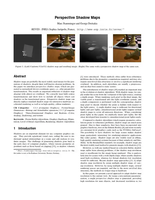
Perspective Shadow MapsMarc Stamminger and George DrettakisREVES -INRIA Sophia-Antipolis,France,http://www-sop.inria.fr/reves/Figure 1:(Left)Uniform 512x512shadow map and resulting image.(Right)The same with a perspective shadow map of the same size.AbstractShadow maps are probably the most widely used means for the gen-eration of shadows,despite their well known aliasing problems.Inthis paper we introduce perspective shadow maps ,which are gen-erated in normalized device coordinate space,i.e.,after perspective transformation.This results in important reduction of shadow map aliasing with almost no overhead.We correctly treat light source transformations and show how to include all objects which cast shadows in the transformed space.Perspective shadow maps can directly replace standard shadow maps for interactive hardware ac-celerated rendering as well as in high-quality,offline renderers.CR Categories:I.3.3[Computer Graphics]:Picture/Image Generation—Bitmap and framebuffer operations;I.3.7[Computer Graphics]:Three-Dimensional Graphics and Realism—Color,shading,shadowing,and textureKeywords:Frame Buffer Algorithms,Graphics Hardware,Illumi-nation,Level of Detail Algorithms,Rendering,Shadow Algorithms1IntroductionShadows are an important element for any computer graphics im-age.They provide significant visual cues,aiding the user to un-derstand spatial relationships in a scene and add realism to syn-thetic images.The challenge of generating shadows goes back to the early days of computer graphics,where various geometric al-gorithms such as those based on clipping [15],or shadow volumesMarc.Stamminger|George.Drettakis @sophia.inria.fr The first author is now at the Bauhaus-Universit¨a t,Weimar,Germany.[1]were introduced.These methods often suffer from robustnessproblems due to the geometric computations required,and may also require non-trivial data structures or involve a significant rendering overhead.In addition,such algorithms are usually a preprocess,and are thus best suited to static scenes.The introduction of shadow maps [16]marked an important step in the evolution of shadow algorithms.With shadow maps,we sim-ply render the scene from the viewpoint of the light source,creating a depth image.When rendering each pixel in the final image,the visible point is transformed into the light coordinate system,and a depth comparison is performed with the corresponding shadow map pixel to decide whether the point is hidden with respect to the light source.A single shadow map is sufficient for directional lights and spot lights;omnidirectional point lights require several shadow maps to cover all emission directions.When considering point lights in this paper,we implicitly mean spot lights,but the ideas developed here transfer to omnidirectional point lights pared to shadow algorithms which require geometric calcu-lations prone to robustness problems,shadow maps are much more general.Due to their simplicity,they have been incorporated into graphics hardware,first on the Infinite Reality [6]and more recently on consumer-level graphics cards such as the NVIDIA GeForce3.The possibility to have shadows for large scenes makes shadow maps particularly interesting for rendering-intensive applications like video games.Shadow maps are also widely used in offline,high-quality rendering systems because of their simplicity and flex-ibility.In the RenderMan standard,for example,shadow maps are the most widely used method to generate images with shadows [13].However,as with any method based on a discrete buffer,shadow maps suffer from aliasing problems,if the shadow map resolution used is insufficient for the image being rendered.This is particu-larly true for scenes with a wide depth range,where nearby shadows need high resolution,whereas for distant shadows low resolution would be sufficient.Recent shadow map approaches [12,2]adapt shadow map resolution by using multiple shadow maps of vary-ing resolution.However,by using multiple shadow maps,several rendering passes are required,and due to the more involved data structures,the methods no longer map to hardware.In this paper,we present a novel approach to adapt shadow map resolution to the current view.By using a non-uniform parameter-ization,a single perspective shadow map is generated,providing high resolution for near objects,and decreased resolution as wemove away from the viewpoint.An example is shown in Fig.1.A standard shadow map(left)has insufficient resolution for nearby objects(center left).In contrast,in our perspective shadow map (center right),resolution varies such that nearby objects have suffi-cient shadow map resolution(right).Our shadow map projection can still be represented by a44 matrix,so that it fully maps to hardware.It can easily be used to improve any interactive and offline rendering method based on shadow maps,with only marginal overhead for the computation of the optimized projection matrix.Perspective shadow maps often re-duce aliasing dramatically.In a few difficult cases,our parameteri-zation converges to standard uniform shadow maps.Our approach is view-dependent,requiring the generation of a new shadow map at each frame or at least after major camera movements.This is necessary for scenes containing moving objects anyhow,such as those used in video games or other interactive applications.In this case,we have no significant speed penalty compared to a standard,fixed-resolution shadow map.1.1Shadow Map AliasingFirst,we briefly formalize the aliasing problems of shadow maps for point light sources.Every pixel in the shadow map represents a sheared pyramid of rays,passing through a shadow map pixel of size d s x d s on the(shadow)image plane(Fig.2).In the follow-ing,we will call the reciprocal of d s the shadow map resolution. To increase shadow map resolution we decrease d s and vice versa. When the ray bundle through a shadow map pixel hits a surface at distance r s under angleα,the size of the intersection is approx-imately d s r s cosα.In thefinal image,this intersection with thesurface has size:d d s r sr icosβcosαwhereβis the angle between the light source direction and the sur-face normal and r i is the distance from the camera to the intersec-tion.Figure2:Shadow map projection quantities.For directional light sources,d is independent of r s,so d onlydepends on d s r i.Analogously,for an orthogonal view d is propor-tional to d s r s.Shadow map undersampling appears when d is larger than theimage pixel size d i.This can happen when d s r s r i becomes large,which typically happens when the user zooms into a shadow bound-ary so that single shadow map pixels become visible.We will callthis perspective aliasing.Due to limited memory,the shadow mapresolution1d s can only be increased up to a certain limit in prac-tice.Perspective aliasing can be avoided by keeping the fractionr s r i close to a constant.As we show in this paper,this is what isachieved when we compute the shadow map after perspective trans-formation.When cosβcosαbecomes large,projection aliasing appears.This typically happens when the light rays are almost parallel to asurface,so that the shadow stretches along the surface.Projectionaliasing is not treated by perspective shadow maps,since this wouldrequire a local increase in shadow map resolution.This is not possi-ble without much more involved data structures,and it would forceus to abandon hardware acceleration.Note that there are also other sources of aliasing when usingshadow maps,e.g.,depth quantization,which we will not treat here.1.2Related WorkThe literature on shadow generation in computer graphics is vast,and far beyond the scope of this paper(see[17]for an old,but nicesurvey).We thus concentrate our review on previous work directlyrelated to shadows maps and our novel approach.Reeves et al.[9]introduced the concept of percentage closerfil-tering.The idea is tofilter the shadows obtained from shadow mapsby interpolating the binary result of the depth comparison insteadof the depth values.The deep shadow maps of Lokovic et al.[5]extend the idea offiltering shadow maps by storing approximateattenuation functions for each shadow map pixel,thus capturingself shadowing within hair,fur or smoke.Both approaches performanti-aliasing in that theyfilter undersampling artifacts,but they donot solve the problem of undersampling as such.Tadamura et al.[12]introduce multiple shadow maps with vary-ing resolution as a solution to the aliasing problem for large outdoorscenes.This solves the problem of perspective aliasing,but it doesnot map to hardware and is thus not appropriate for interactive ap-plications.An interesting improvement to traditional shadow maps is theadaptive shadow map method[2].This approach replaces the“flat”shadow map with an adaptive,hierarchical representation,which isupdated continuously during a walkthrough.For each frame,afirstrendering pass is required to determine which parts of the hierarchi-cal shadow map need refinement.This is achieved using OpenGLtexture mip-mapping capabilities.Perspective and projection alias-ing are detected.The most critical parts of the shadow map are thenrendered at higher resolution,read back,and inserted into the hier-archical shadow map structure.Oversampled parts of the hierarchyare truncated.The method is a software solution,since it requiresthe traversal and refinement of a hierarchical data structure insteadof a shadow map,and thus cannot entirely map to hardware.Rapidview changes make it necessary to update a large number of nodesin the hierarchy,so either the frame rate drops or aliasing appearsuntil the hierarchical structure has been updated.The generation ofa new node essentially requires an entire rendering pass,albeit witha small part of the model,but with the full cost of a frame-bufferreadback to update the data structure.Scenes with moving objectswould require the generation of the entire hierarchical structure ateach frame,which would require many rendering passes.Shadow maps are closely related to textures,so we assume thereader is familiar with the texturing and the projective mapping pro-cess.Most standard graphics textbooks treat these issues[3].Aparticularly nice and thorough description can be found in[4].2OverviewPerspective shadow maps are computed in post-perspective spaceof the current camera,or,using standard graphics terminology,thespace of normalized device coordinates[3].In the traditional ren-dering pipeline,perspective is obtained by transforming the worldto a perspectively distorted space,where objects close to the cameraare enlarged and distant objects are shrunk(see Fig.3).This map-ping is projective[4]and can thus be represented by a44ma-trix with homogeneous coordinates.It projects the current viewingfrustum to the unit cube;thefinal image is generated by a parallelprojection of this cube along z.The idea of perspective shadow maps is tofirst map the sceneto post-perspective space and then generate a standard shadowmap in this space by rendering a view from the transformed light source to the unit cube.We can work in post-perspective space al-most as in world space,with the exception of objects behind the viewer,which will be handled in Sect.4.Because the shadow map “sees”the scene after perspective projection,perspective aliasing (see Sect.1.1)is significantly decreased,if not completely avoided.To explain this principle a special case is depicted in Fig.3.The scene is illuminated by a vertical directional light source.In post-perspective space the shadow map is an orthogonal view from the top onto the unit cube and the final image is an orthogonal view from the front.Consequently,all shadow map pixels projected onto the ground in this scene have the same size in the image.Thus,in the sense of Sect.1.1,perspective aliasing is completely avoided for thiscase.Figure 3:The scene is illuminated by a vertical directional light source (left).By applying the eye-view perspective transformation and then generating the shadow map (right),the shadow map pixels projected on the ground are evenly distributed in the image.3Post-Perspective Light SourcesTo apply our new method,we first transform the scene to post-perspective space,using the camera matrix.We then transform the light source by the same matrix,and generate the shadow map.The different cases which arise are described next.3.1Directional Light SourcesDirectional light sources can be considered as point lights at infin-ity.The perspective mapping can move these sources to a finite position;the set of possible cases is shown in Fig.3and 4.A di-rectional light source parallel to the image plane remains at infinity.All other directional light sources become point lights on the infin-ity plane at z f n f n ,where n and f are the near and far distance of the viewing frustum (see Fig.3).A directional light source shining from the front becomes a point light in post-perspective space (Fig.4,left),whereas a directional light source from behind is mapped to a “inverted”point light source (center).In this context,“inverted”means that all light rays for these light sources do not emanate,but converge to a single point.Such inverted point light sources can easily be handled as point lights with their shadow map depth test reversed,such that hit points furthest from the point source survive.The extreme cases are directional lights parallel (facing or opposite to)the view direction,which are mapped to a point light just in front of the viewer (right).3.2Point Light SourcesThe different settings for point light sources are shown in Fig.5.Point light sources in front of the viewer remain point lights,(left).Figure 4:Directional lights in world space (top row)become point lights in post perspective space (bottom row)on the infinity plane.Lights from behind become inverted,i.e.,the order of hits along a ray isinverted.Figure 5:Mapping of point lights in world space (top row)to post-perspective space (bottom row).A point light in front of the user remains a normal point light (left),a point light behind the viewer becomes inverted (center).Boundary cases are mapped to direc-tional lights (right).Point lights behind the viewer are mapped beyond the infinity plane and become inverted (center).Point lights on the plane through the view point which is perpendicular to the view direction (camera plane),however,become directional (right).3.3DiscussionIn post-perspective space,the final image is an orthogonal view onto the unit cube.Following our observations in Sect.1.1,this means that perspective aliasing due to distance to the eye,r i ,is avoided.However,if the light source is mapped to a point light in post-perspective space,aliasing due to the distance to the shadow map image plane,r s ,can appear.The ideal case occurs when,after the perspective mapping,the light source is directional.Perspective aliasing due to r s is thus also avoided.This happens for:a directional light parallel to the image plane (see Fig.3),a point light in the camera plane.The typical example is the miner’s head-lamp,that is a point light just above the camera.It is known that this setting is also ideal for standard shadow maps [7].With our parameterization,the offset can be arbi-trarily large,as long as the point remains in the camera plane.On the other hand,the less optimal cases appear when we obtain a point light with a large depth range in post-perspective space.Theextreme example is a directional light parallel to the viewing direc-tion.In post-perspective space,this becomes a point light on the in-finity plane on the opposite side of the viewer (see Fig.4right).In this worst case the two perspective projections with opposite view-ing directions cancel out mutually and we obtain a standard uniform shadow map.In general,for directional light sources the benefit is maximal for a light direction perpendicular to the view direction.Since these are also parallel lights in post-perspective space,perspective aliasing is completely avoided in this case.Consider the smaller of the two angles formed between the light direction and the viewing direc-tion.The benefit of our approach decreases as this angle becomes smaller,since we move further away from the ideal,perpendicu-lar case.If the angle is zero our parameterization corresponds to a uniform shadow map.For point lights,the analysis is harder,since the point light source also applies a perspective rmally,the ad-vantage of our parameterization is largest when the point light is far away from the viewing frustum,so that it is similar to a paral-lel light,and if the visible illuminated region exhibits a large depth range.For the case of a miner’s lamp,which is known to be ideal for uniform shadow maps [7],our parameterization again converges to the uniform setting.A common problem in shadow maps is the bias necessary to avoid self-occlusion or surface acne [7].This problem is in-creased for perspective shadow maps,because objects are scaled non-uniformly.We use a constant offset in depth in shadow map space,which may require user adjustment depending on the scene.4Including all Objects Casting ShadowsUp to now,we ignored an important issue:our shadow map is op-timized for the current viewing frustum.But the shadow map must contain all objects within that frustum plus all potential occluders outside the frustum that can cast a shadow onto any visible object.4.1World SpaceMore formally,we define the set of points that must appear in the shadow map as follows:Let S be an envelope of the scene objects,typically its bounding box.V is the viewing frustum and L the light source frustum.The light source is at position l (for directional lights L R 3and l is at infinity).First,we compute the convex hull M of V and l ,so M contains all rays from points in V to l .From M we then remove all points outside the scene’s bounding box and the light frustum:H M S L (shown in yellow in Fig.6(right)).Figure 6:The current view frustum V ,the light frustum with light position l ,and the scene bounding box S (left).M is obtained by extending V towards the light (center).Then M is intersected with S and L to obtain the set of points that need to be visible in the shadow map (right).In our implementation we use the computational geometry li-brary CGAL ( )to perform these geometric com-putations.As a result,the window of the shadow map is chosen sothat all points in H are included.However,the shadow map will not see H ,but its transformation to post-perspective space,so we have to consider how H changes by the perspective mapping.4.2Post-perspective SpaceUnder projective transformations lines remain lines,but the order of points along a line can change.For perspective projections,this happens when a line intersects the camera plane,where the inter-section point is mapped to infinity.As a result,we can quickly transform the convex set H to post-perspective space by transfor-mation of its vertices,as long as H is completely in front of the viewer.An example where this is not the case is shown in Fig.7.Points behind the viewer had to be included,because they can cast shadows into the viewing frustum.However,in post-perspective space,these points are projected to beyond the infinity plane.In this case,possible occluders can be on both sides of the infinityplane.by source behind (top left).After perspective projection,an object behind the viewer is inverted and appears on the other side of the infinity plane (lower left).To treat this we move the center of projection back (upper right),so that we are behind the furthermost point which can cast a shadow into the view frustum.After this,a standard shadow map in post-perspective space is again sufficient (lower right).One solution would be to generate two shadow maps in this case.A first one as described previously,and a second one that looks “beyond”the infinity plane.We avoid this awkward solution by a virtual camera shift.We virtually move the camera view point backwards,such that H lies entirely inside the transformed cam-era frustum;the near plane distance remains unchanged and the far plane distance is increased to contain the entire previous frustum.Note that this camera point displacement is only for the shadow map generation,not for rendering the image.By this,we modify the post-perspective space,resulting in de-creased perspective foreshortening.If we move the camera to infin-ity,we obtain an orthogonal view with a post-perspective space that is equivalent to the original world space;the resulting perspective shadow map then corresponds to a standard uniform shadow map.Consequently,we can say that by moving back the camera,our parameterization degrades towards that of a standard shadow map.By this,perspective aliasing is reintroduced,however,in practice this is only relevant for extreme cases,so we found it preferable to the double shadow map solution.It is interesting to note that for the cases that are ideal for perspective shadow maps,no such shift is necessary,because H will always be completely in front of the camera.The shift distance will be significant only if the light source is far behind the viewer.But in this case,our parameterization con-verges to the uniform shadow map anyway.5Point RenderingPoint rendering(e.g.,[8,10,11,14])has proven to be a very effec-tive means for rendering complex geometry.Points are particularly well suited for natural objects.However,for the generation of uni-form shadow maps point rendering loses most of its benefits.A very large,dense point set needs to be generated in order to render a high-resolution uniform shadow map.Frequent regeneration of the shadow map for dynamic scenes becomes highly inefficient.On the other hand,our projective shadow map parameterization fits nicely with the point rendering approaches presented in[14,11], in the sense that the point sets generated by these methods can also be used for the rendering of the shadow map.The reason is that these approaches generate random point clouds,with point den-sities adapted to the distance to the viewer.In post-perspective space,these point clouds have uniform point density.Since per-spective shadow maps are rendered in this space,the shadow map can assume that point densities are uniform.It is thus easy to select the splat size when rendering the shadow map such that holes are avoided.6Implementation and ResultsWe implemented perspective shadow maps within an inter-active rendering application using OpenGL hardware assisted shadow maps.The following results,and all sequences on the accompanying video,were obtained under Linux on a Compaq AP550with two1GHz Pentium III processors and an NVIDIA GeForce3graphics accelerator.We used the shadow map extensions GL SGIX depth texture and GL SGIX shadow.The shadow maps are rendered into p-buffers (GLX SGIX pbuffer)and are applied using register combiners (GL NV register combiners).In order to obtain optimal results from perspective shadow maps, we require that the near plane of the view be as far as possible. We achieve this by reading back the depth buffer after each frame, searching the minimal depth value,and adapting the near plane ac-cordingly.Due to the fast bus and RAM of our computer,the speed penalty for reading back the depth buffer is moderate,e.g.,10ms for reading back depth with16bits precision at640by480pixel resolution.The increase in quality is well worth this overhead.Fig.1shows a chess board scene,lit by a spot light source.The left image shows a uniform shadow map,the center left image is the resulting rendering with well visible shadow map aliasing.The far right image was obtained with a perspective shadow map of the same size,which is shown on the center right.Fig.8shows Notre Dame in Paris,augmented with a crowd and trees.With point based rendering for the trees and the crowd,the views shown are still obtained at about15frames/sec.In the street scene in Fig.9the cars and two airplanes are mov-ing.Thefigure shows three snapshots from an interactive session; all images were obtained at more than ten frames per second with perspective shadow maps of size10241024.Ourfinal test scene is a complete ecosystem,consisting of hun-dreds of different plants and a few cows.The view shown in Fig.10contains more than20million triangles.We show the image without shadows(left),with shadows from a10241024uniform shadow map(center)and with shadows from a projective shadow map of the same size(right).7ConclusionsWe have introduced perspective shadow maps,a novel parameter-ization for shadow maps.Our approach permits the generation of shadow maps with greatly improved quality,compared to standard uniform shadow maps.By choosing an appropriate projective map-ping,shadow map resolution is concentrated where appropriate.We have also shown how our method can be used for point rendering, thus allowing interactive display of very complex scenes with high-quality shadows.Perspective shadow maps can be used in interac-tive applications and fully exploit shadow map capabilities of recent graphics hardware,but they are also applicable to high-quality soft-ware renderers.8AcknowledgmentsThefirst author has been supported by a Marie-Curie postdoctoral Fellowship while doing this work.L.Kettner implemented the frus-tum intersection code in CGAL().Thanks to F.Durand for his very helpful comments.Most of the models in the result section were downloaded from and .References[1] F.C.Crow.Shadow algorithms for computer puterGraphics(Proc.of SIGGRAPH77),11(2):242–248,1977.[2]R.Fernando,S.Fernandez,K.Bala,and D.P.Greenberg.Adaptiveshadow maps.Proc.of SIGGRAPH2001,pages387–390,2001. [3]J.D.Foley,A.van Dam,S.K.Feiner,and putergraphics,principles and practice,second edition.1990.[4]P.Heckbert.Survey of Texture Mapping.IEEE Computer Graphicsand Applications,6(11):56–67,November1986.[5]T.Lokovic and E.Veach.Deep shadow maps.Proc.of SIGGRAPH2000,pages385–392,2000.[6]J.S.Montrym,D.R.Baum,D.L.Dignam,and C.J.Migdal.Infinite-reality:A real-time graphics system.Proc.of SIGGRAPH97,pages 293–302,1997.[7]nvidia.webpage./view.asp?IO=cedec shadowmap.[8]H.Pfister,M.Zwicker,J.van Baar,and M.Gross.Surfels:Surfaceelements as rendering primitives.Proc.of SIGGRAPH2000,pages 335–342,2000.[9]W.T.Reeves,D.H.Salesin,and R.L.Cook.Rendering antialiasedshadows with depth puter Graphics(Proc.of SIGGRAPH87),21(4):283–291,1987.[10]S.Rusinkiewicz and M.Levoy.Qsplat:A multiresolution point ren-dering system for large meshes.Proc.of SIGGRAPH2000,pages 343–352,2000.[11]M.Stamminger and G.Drettakis.Interactive sampling and ren-dering for complex and procedural geometry.In S.Gortler and K.Myszkowski,editors,Rendering Techniques2001(12th Euro-graphics Workshop on Rendering),pages151–162.Springer Verlag, 2001.[12]K.Tadamura,X.Qin,G.Jiao,and E.Nakamae.Rendering optimal so-lar shadows with plural sunlight depth buffers.The Visual Computer, 17(2):76–90,2001.[13]S.Upstill.The RenderMan Companion.Addison-Wesley,1990.[14]M.Wand,M.Fischer,I.Peter,F.Meyer auf der Heide,and W.Straßer.The randomized z-buffer algorithm:Interactive rendering of highly complex scenes.Proc.of SIGGRAPH2001,pages361–370,2001. [15]K.Weiler and K.Atherton.Hidden surface removal using poly-gon area puter Graphics(Proc.of SIGGRAPH77), 11(2):214–222,1977.[16]L.Williams.Casting curved shadows on curved puterGraphics(Proc.of SIGGRAPH78),12(3):270–274,1978.[17] A.Woo,P.Poulin,and A.Fournier.A survey of shadow algorithms.IEEE Computer Graphics and Applications,10(6):13–32,November 1990.。

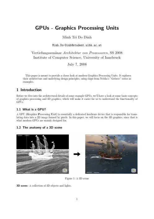
GPUs-Graphics Processing UnitsMinh Tri Do DinhMinh.Do-Dinh@student.uibk.ac.atVertiefungsseminar Architektur von Prozessoren,SS2008Institute of Computer Science,University of InnsbruckJuly7,2008This paper is meant to provide a closer look at modern Graphics Processing Units.It explorestheir architecture and underlying design principles,using chips from Nvidia’s”Geforce”series asexamples.1IntroductionBefore we dive into the architectural details of some example GPUs,we’ll have a look at some basic concepts of graphics processing and3D graphics,which will make it easier for us to understand the functionality of GPUs1.1What is a GPU?A GPU(G raphics P rocessing U nit)is essentially a dedicated hardware device that is responsible for trans-lating data into a2D image formed by pixels.In this paper,we will focus on the3D graphics,since that is what modern GPUs are mainly designed for.1.2The anatomy of a3D sceneFigure1:A3D scene3D scene:A collection of3D objects and lights.Figure2:Object,triangle and vertices3D objects:Arbitrary objects,whose geometry consists of triangular polygons.Polygons are composed of vertices.Vertex:A Point with spatial coordinates and other information such as color and texture coordinates.Figure3:A cube with a checkerboard textureTexture:An image that is mapped onto the surface of a3D object,which creates the illusion of an object consisting of a certain material.The vertices of an object store the so-called texture coordinates (2-dimensional vectors)that specify how a texture is mapped onto any given surface.Figure4:Texture coordinates of a triangle with a brick textureIn order to translate such a3D scene to a2D image,the data has to go through several stages of a”Graphics Pipeline”1.3The Graphics PipelineFigure5:The3D Graphics PipelineFirst,among some other operations,we have to translate the data that is provided by the application from 3D to2D.1.3.1Geometry StageThis stage is also referred to as the”Transform and Lighting”stage.In order to translate the scene from 3D to2D,all the objects of a scene need to be transformed to various spaces-each with its own coordinate system-before the3D image can be projected onto a2D plane.These transformations are applied on a vertex-to-vertex basis.Mathematical PrinciplesA point in3D space usually has3coordinates,specifying its position.If we keep using3-dimensional vectors for the transformation calculations,we run into the problem that different transformations require different operations(e.g.:translating a vertex requires addition with a vector while rotating a vertex requires multiplication with a3x3matrix).We circumvent this problem simply by extending the3-dimensional vector by another coordinate(the w-coordinate),thus getting what is called homogeneous coordinates.This way, every transformation can be applied by multiplying the vector with a specific4x4matrix,making calculations much easier.Figure6:Transformation matrices for translation,rotation and scalingLighting,the other major part of this pipeline stage is calculated using the normal vectors of the surfaces of an object.In combination with the position of the camera and the position of the light source,one can compute the lighting properties of a given vertex.Figure7:Calculating lightingFor transformation,we start out in the model space where each object(model)has its own coordinate system,which facilitates geometric transformations such as translation,rotation and scaling.After that,we move on to the world space,where all objects within the scene have a unified coordinate system.Figure8:World space coordinatesThe next step is the transformation into view space,which locates a camera in the world space and then transforms the scene,such that the camera is at the origin of the view space,looking straight into the positive z-direction.Now we can define a view volume,the so-called view frustrum,which will be used to decide what actually is visible and needs to be rendered.Figure9:The camera/eye,the view frustrum and its clipping planesAfter that,the vertices are transformed into clip space and assembled into primitives(triangles or lines), which sets up the so-called clipping process.While objects that are outside of the frustrum don’t need to be rendered and can be discarded,objects that are partially inside the frustrum need to be clipped(hence the name),and new vertices with proper texture and color coordinates need to be created.A perspective divide is then performed,which transforms the frustrum into a cube with normalized coordinates(x and y between-1and1,z between0and1)while the objects inside the frustrum are scaled accordingly.Having this normalized cube facilitates clipping operations and sets up the projection into2D space(the cube simply needs to be”flattened”).Figure10:Transforming into clip spaceFinally,we can move into screen space where x and y coordinates are transformed for proper2D display (in a given window).(Note that the z-coordinate of a vertex is retained for later depth operations)Figure11:From view space to screen spaceNote,that the texture coordinates need to be transformed as well and additionally besides clipping,sur-faces that aren’t visible(e.g.the backside of a cube)are removed as well(so-called back face culling).The result is a2D image of the3D scene,and we can move on to the next stage.1.3.2Rasterization StageNext in the pipeline is the Rasterization stage.The GPU needs to traverse the2D image and convert the data into a number of”pixel-candidates”,so-called fragments,which may later become pixels of the final image.A fragment is a data structure that contains attributes such as position,color,depth,texture coordinates,etc.and is generated by checking which part of any given primitive intersects with which pixel of the screen.If a fragment intersects with a primitive,but not any of its vertices,the attributes of that fragment have to be additionally calculated by interpolating the attributes between the vertices.Figure12:Rasterizing a triangle and interpolating its color valuesAfter that,further steps can be made to obtain thefinal pixels.Colors are calculated by combining textures with other attributes such as color and lighting or by combining a fragment with either another translucent fragment(so-called alpha blending)or optional fog(another graphical effect).Visibility checks are performed such as:•Scissor test(checking visibility against a rectangular mask)•Stencil test(similar to scissor test,only against arbitrary pixel masks in a buffer)•Depth test(comparing the z-coordinate of fragments,discarding those which are further away)•Alpha test(checking visibility against translucent fragments)Additional procedures like anti-aliasing can be applied before we achieve thefinal result:a number of pixels that can be written into memory for later display.This concludes our short tour through the graphics pipeline,which hopefully gives us a better idea of what kind of functionality will be required of a GPU.2Evolution of the GPUSome historical key points in the development of the GPU:•Efforts for real time graphics have been made as early as1944(MIT’s project”Whirlwind”)•In the1980s,hardware similar to modern GPUs began to show up in the research community(“Pixel-Planes”,a a parallel system for rasterizing and texture-mapping3D geometry•Graphic chips in the early1980s were very limited in their functionality•In the late1980s and early1990s,high-speed,general-purpose microprocessors became popular for implementing high-end GPUs(e.g.Texas Instruments’TMS340)•1985Thefirst mass-market graphics accelerator was included in the Commodore Amiga•1991S3introduced thefirst single chip2D-accelerator,the S386C911•1995Nvidia releases one of thefirst3D accelerators,the NV1•1999Nvidia’s Geforce256is thefirst GPU to implement Transform and Lighting in Hardware •2001Nvidia implements thefirst programmable shader units with the Geforce3•2005ATI develops thefirst GPU with unified shader architecture with the ATI Xenos for the XBox 360•2006Nvidia launches thefirst unified shader GPU for the PC with the Geforce88003From Theory to Practice-the Geforce68003.1OverviewModern GPUs closely follow the layout of the graphics pipeline described in thefirst ing Nvidia’s Geforce6800as an example we will have a closer look at the architecture of modern day GPUs.Since being founded in1993,the company NVIDIA has become one of the biggest manufacturers of GPUs (besides ATI),having released important chips such as the Geforce256,and the Geforce3.Launched in2004,the Geforce6800belongs to the Geforce6series,Nvidia’s sixth generation of graphics chipsets and the fourth generation that featured programmability(more on that later).The following image shows a schematic view of the Geforce6800and its functional units.Figure13:Schematic view of the Geforce6800You can already see how each of the functional units correspond to the stages of the graphics pipeline. We start with six parallel vertex processors that receive data from the host(the CPU)and perform oper-ations such as transformation and lighting.Next,the output goes into the triangle setup stage which takes care of primitive assembly,culling and clipping,and then into the rasterizer which produces the fragments.The Geforce6800has an additional Z-cull unit which allows to perform an early fragment visibility check based on depth,further improving the efficiency.We then move on to the sixteen fragment processors which operate in4parallel units and computes the output colors of each fragment.The fragment crossbar is a linking element that is basically responsible for directing output pixels to any available pixel engine(also called ROP,short for R aster O perator),thus avoiding pipeline stalls.The16pixel engines are thefinal stage of processing,and perform operations such as alpha blending, depth tests,etc.,before delivering thefinal pixel to the frame buffer.3.2In DetailFigure14:A more detailed view of the Geforce6800While most parts of the GPU arefixed function units,the vertex and fragment processors of the Geforce 6800offer programmability which wasfirst introduced to the geforce chipset line with the geforce3(2001). We’ll have a more detailed look at the units in the following sections.3.2.1Vertex ProcessorFigure15:A vertex processorThe vertex processors are the programmable units responsible for all the vertex transformations and at-tribute calculations.They operate with4-dimensional data vectors corresponding with the aforementioned homogeneous coordinates of a vertex,using32bits per coordinate(hence the128bits of a register).Instruc-tions are123bits long and are stored in the Instruction RAM.The data path of a vertex processor consists of:•A multiply-add unit for4-dimensional vectors•A scalar special function unit•A texture unitInstruction set:Some notable instructions for the vertex processor include:dp4dst,src0,src1Computes the four-component dot product of the source registersexp dst,src Provides exponential2xdst dest,src0,src1Calculates a distance vectornrm dst,src Normalize a3D vectorrsq dst,src Computes the reciprocal square root(positive only)of the sourcescalarRegisters in the vertex processor instructions can be modified(with few exceptions):•Negate the register value•Take the absolute value of the register•Swizzling(copy any source register component to any temporary register component)•Mask destination register componentsOther technical details:•Vertex processors are MIMD units(Multiple Instruction Multiple Data)•They use VLIW(Very Long Instruction Words)•They operate with32-bitfloating point precision•Each vertex processor runs up to3threads to hide latency•Each vertex processor can perform a four-wide MAD(Multiply-Add)and a special function in one cycle3.2.2Fragment ProcessorFigure16:A fragment processorThe Geforce6800has16fragment processors.They are grouped to4bigger units which operate simulta-neously on4fragments each(a so-called quad).They can take position,color,depth,fog as well as other arbitrary4-dimensional attributes as input.The data path consists of:•An Interpolation block for attributes•2vector math(shader)units,each with slightly different functionality•A fragment texture unitSuperscalarity:A fragment processor works with4-vectors(vector-oriented instruction set),where sometimes components of the vector need be treated seperately(e.g.color,alpha).Thus,the fragment processor supports co-issueing of the data,which means splitting the vector into2parts and executing different operations on them in the same clock.It supports3-1and2-2splitting(2-2co-issue wasn’t possible earlier).Additionally,it also features dual issue,which means executing different operations on the2vector math units in the same clock.Texture Unit:The texture unit is afloating-point texture processor which fetches andfilters the texture data.It is con-nected to a level1texture cache(which stores parts of the textures that are used).Shader units1and2:Each shader unit is limited in its abilities,offering complete functionality when used together.Figure17:Block diagram of Shader Unit1and2Shader Unit1:Green:A crossbar which distributes the input coming eiter from the rasterizer or from the loopback Red:InterpolatorsYellow:A special function unit(for functions such as Reciprocal,Reciprocal Square Root,etc.)Cyan:MUL channelsOrange:A unit for texture operations(not the fragment texture unit)The shader unit can perform2operations per clock:A MUL on a3-dimensional vector and a special function,a special function and a texture operation,or2 MULs.The output of the special function unit can go into the MUL channels.The texture gets input from the MUL unit and does LOD(Level Of Detail)calculations,before passing the data to the actual fragment texture unit.The fragment texture unit then performs the actual sampling and writes the data into registers for the second shader unit.The shader unit can simply pass data as well.Shader Unit2:Red:A crossbarCyan:4MUL channelsGray:4ADD channelsYellow:1special function unitThe crossbar splits the input onto5channels(4components,1channel stays free).The ADD units are additionally connected,allowing advanced operations such as a dotproduct in one clock. Again,the shader unit can handle2independent operations per cycle or it can simply pass data.If no special function is used,the MAD unit can perform up to2operations from this list:MUL,ADD,MAD,DP,or any other instruction based on these operations.Instruction set:Some notable instructions for the vertex processor include:cmp dst,src0,src1,src2Choose src1if src0>=0.Otherwise,choose src2.The comparisonis done per channeldsx dst,src Compute the rate of change in the render target’s x-directiondsy dst,src Compute the rate of change in the render target’s y-direction sincos dst.{x|y|xy},src0.{x|y|z|w}Computes sine and cosine,in radianstexld dst,src0,src1Sample a texture at a particular sampler,using provided texturecoordinatesRegisters in the fragment processor instructions can be modified(with few exceptions):•Negate the register value•Take the absolute value of the register•Mask destination register componentsOther technical details:•The fragment processors can perform operations within16or32floating point precision(e.g.the fog unit uses only16bit precision for its calculations since that is sufficient)•The quads operate as SIMD units•They use VLIW•They run up to100s of threads to hide texture fetch latency(˜256per quad)•A fragment processor can perform up to8operations per cycle/4math operations if there’s a texture fetch in shader1Figure18:Possible operations per cycle•The fragment processors have a2level texture cache•The fog unit can perform fog blending on thefinal pass without performance penalty.It is implemented withfixed point precision since that’s sufficient for fog and saves performance.The equation:out=FogColor*fogFraction+SrcColor*(1-fogFraction)•There’s support for multiple render targets,the pixel processor can output to up to four seperate buffers(4x4values,color+depth)3.2.3Pixel EngineFigure19:A pixel engineLast in the pipeline are the16pixel engines(raster operators).Each pixel engine connects to a specific memory partition of the GPU.After the lossless color and depth compression,the depth and color units perform depth,color and stencil operations before writing thefinal pixel.When activated the pixel engines also perform multisample antialiasing.3.2.4MemoryFrom“GPU Gems2,Chapter30:The GeForce6Series GPU Architecture”:“The memory system is partitioned into up to four independent memory partitions,eachwith its own dynamic random-access memories(DRAMs).GPUs use standard DRAM modulesrather than custom RAM technologies to take advantage of market economies and thereby reducecost.Having smaller,independent memory partitions allows the memory subsystem to operateefficiently regardless of whether large or small blocks of data are transferred.All rendered surfacesare stored in the DRAMs,while textures and input data can be stored in the DRAMs or insystem memory.The four independent memory partitions give the GPU a wide(256bits),flexible memory subsystem,allowing for streaming of relatively small(32-byte)memory accessesat near the35GB/sec physical limit.”3.3Performance•425MHz internal graphics clock•550MHz memory clock•256-MB memory size•35.2GByte/second memory bandwidth•600million vertices/second•6.4billion texels/second•12.8billion pixels/second,rendering z/stencil-only(useful for shadow volumes and shadow buffers)•6four-wide fp32vector MADs per clock cycle in the vertex shader,plus one scalar multifunction operation(a complex math operation,such as a sine or reciprocal square root)•16four-wide fp32vector MADs per clock cycle in the fragment processor,plus16four-wide fp32 multiplies per clock cycle•64pixels per clock cycle early z-cull(reject rate)•120+Gflops peak(equal to six5-GHz Pentium4processors)•Up to120W energy consumption(the card has two additional power connectors,the power sources are recommended to be no less than480W)4Computational PrinciplesStream Processing:Typical CPUs(the von Neumann architecture)suffer from memory bottlenecks when processing.GPUs are very sensitive to such bottlenecks,and therefore need a different architecture,they are essentially special purpose stream processors.A stream processor is a processor that works with so-called streams and kernels.A stream is a set of data and a kernel is a small program.In stream processors,every kernel takes one or more streams as input and outputs one or more streams,while it executes its operations on every single element of the input streams. In stream processors you can achieve several levels of parallelism:•Instruction level parallelism:kernels perform hundreds of instructions on every stream element,you achieve parallelism by performing independent instructions in parallel•Data level parallelism:kernels perform the same instructions on each stream element,you achieve parallelism by performing one instruction on many stream elements at a time•Task level parallelism:Have multiple stream processors divide the work from one kernelStream processors do not use caching the same way traditional processors do since the input datasets are usually much larger than most caches and the data is barely reused-with GPUs for example the data is usually rendered and then discarded.We know GPUs have to work with large amounts of data,the computations are simpler but they need to be fast and parallel,so it becomes clear that the stream processor architecture is very well suited for GPUs. Continuing these ideas,GPUs employ following strategies to increase output:Pipelining:Pipelining describes the idea of breaking down a job into multiple components that each perform a single task.GPUs are pipelined,which means that instead of performing complete processing of a pixel before moving on to the next,youfill the pipeline like an assembly line where each component performs a task on the data before passing it to the next stage.So while processing a pixel may take multiple clock cycles,you still achieve an output of one pixel per clock since youfill up the whole pipe.Parallelism:Due to the nature of the data-parallelism can be applied on a per-vertex or per-pixel basis -and the type of processing(highly repetitive)GPUs are very suitable for parallelism,you could have an unlimited amount of pipelines next to each other,as long as the CPU is able to keep them busy.Other GPU characteristics:•GPUs can afford large amounts offloating point computational power since they have lower control overhead•They use dedicated functional units for specialized tasks to increase speeds•GPU memory struggles with bandwidth limitations,and therefore aims for maximum bandwidth usage, employing strategies like data compression,multiple threads to cope with latency,scheduling of DRAM cycles to minimize idle data-bus time,etc.•Caches are designed to support effective streaming with local reuse of data,rather than implementinga cache that achieves99%hit rates(which isn’t feasible),GPU cache designs assume a90%hit ratewith many misses inflight•GPUs have many different performance regimes all with different characteristics and need to be de-signed accordingly4.1The Geforce6800as a general processorYou can see the Geforce6800as a general processor with a lot offloating-point horsepower and high memory bandwidth that can be used for other applications as well.Figure20:A general view of the Geforce6800architectureLooking at the GPU that way,we get:•2serially running programmable blocks with fp32capability.•The Rasterizer can be seen as a unit that expands the data into interpolated values(from one data-”point”to multiple”fragments”).•With MRT(Multiple Render Targets),the fragment processor can output up to16scalarfloating-point values at a time.•Several possibilities to control the dataflow by using the visibility checks of the pixel engines or the Z-cull unit5The next step:the Geforce8800After the Geforce7series which was a continuation of the Geforce6800architecture,Nvidia introduced the Geforce8800in2006.Driven by the desire to increase performance,improve image quality and facilitate programming,the Geforce8800presented a significant evolution of past designs:a unified shader architec-ture(Note,that ATI already used this architecture in2005with the XBOX360GPU).Figure21:From dedicated to unified architectureFigure22:A schematic view of the Geforce8800The unified shader architecture of the Geforce8800essentially boils down to the fact that all the different shader stages become one single stage that can handle all the different shaders.As you can see in Figure22,instead of different dedicated units we now have a single streaming processor array.We have familiar units such as the raster operators(blue,at the bottom)and the triangle setup, rasterization and z-cull unit.Besides these units we now have several managing units that prepare and manage the data as itflows in the loop(vertex,geometry and pixel thread issue,input assembler and thread processor).Figure23:The streaming processor arrayThe streaming processor array consists of8texture processor clusters.Each texture processor cluster in turn consists of2streaming multiprocessors and1texture pipe.A streaming multiprocessor has8streaming processors and2special function units.The streaming pro-cessors work with32-bit scalar data,based on the idea that shader programs are becoming more and more scalar,making a vector architecture more inefficient.They are driven by a high-speed clock that is seperate from the core clock and can perform a dual-issued MUL and MAD at each cycle.Each multiprocessor can have768hardware scheduled threads,grouped together to24SIMD”warps”(A warp is a group of threads). The texture pipe consists of4texture addressing and8texturefiltering units.It performs texture prefetching andfiltering without consuming ALU resources,further increasing efficency.It is apparent that we gain a number of advanteges with such a new architecture.For example,the old problem of constantly changing workload and one shader stage becoming a processing bottleneck is solved since the units can adapt dynamically,now that they are unified.Figure24:Workload balancing with both architecturesWith a single instruction set and the support of fp32throughout the whole pipeline,as well as the support of new data types(integer calculations),programming the GPU now becomes easier as well.6General Purpose Programming on the GPU-an exampleWe use the bitonic merge sort algorithm as an example for efficiently implementing algorithms on a GPU. Bitonic merge sort:Bitonic merge sort works by repeatedly building bitonic lists out of a set of elements and sorting them.A bitonic list is a concatenation of two monotonic lists,one ascending and one descending.E.g.:List A=(3,4,7,8)List B=(6,5,2,1)List AB=(3,4,7,8,6,5,2,1)is a bitonic listList BA=(6,5,2,1,3,4,7,8)is also a bitonic listBitonic lists have a special property that is used in bitonic mergesort:Suppose you have a bitonic list of length2n.You can rearrange the list so that you get two halves with n elements where each element(i)of thefirst half is less than or equal to each corresponding element(i+n)in the second half(or greater than or equal,if the list descendsfirst and then ascends)and the new list is again a bitonic list.This happens by com-paring the corresponding elements and switching them if necessary.This procedure is called a bitonic merge. Bitonic merge sort works by recursively creating and merging bitonic lists that increase in their size until we reach the maximum size and the complete list is sorted.Figure25illustrates the process:Figure25:The different stages of the algorithmThe sorting process has a certain number of stages where comparison passes are performed.Each new stage increases the number of passes by one.This results in bitonic mergesort having a complexity of O(n log2(n)+log(n))which is worse than quicksort,but the algorithm has no worst-case scenario(where quicksort reaches O(n2).The algorithm is very well suited for a GPU.Many of the operations can be performed in parallel and the length stays constant,given a certain number of elements.Now when implementing this algorithm on the GPU,we want to make use of as many resources as possible(both in parallel as well as vertically alongthe pipeline),especially considering that the GPU has shortcomings as well,such as the lack of support for binary or integer operations.For example,simply letting the fragment processor stage handle all the calculations might work,but leaving all the other units unused is a waste of precious resources.A possible solution looks like this:In this algorithm,we have groups of elements(fragments)that have the same sorting conditions,while groups next to each other operate in opposite.Now if we draw a vertex quad over two adjacent groups and set appropriateflags at each corner,we can easily determine group membership by using the rasterizer.For example,if we set the left corners to-1and the right corners to+1,we can check where a fragment belongs to by simply looking at its sign(the interpolation process takes care of that).Figure26:Using vertexflags and the interpolator to determine compare operationsNext,we need to determine which compare operation to use and we need to locate the partner item to compare.Both can again be accomplished by using theflag value.Setting the compare operation to less-than and multiplying with theflag value implicitlyflips the operation to greater-equal halfway across the quad. Locating the partner item happens by multiplying the sign of theflag with an absolute value that specifies the distance between the items.In order to sort elements of an array,we store them in a2D texture.Each row is a set of elements and becomes its own bitonic sequence that needs to be sorted.If we extend the quads over the rows of the2D texture and use the interpolation,we can modulate the comparison so the rows get sorted either up or down according to their row number.This way,pairs of rows become bitonic sequences again which can besorted in the same way we sorted the columns of the single rows,simply by transposing the quads.As afinal optimization we reduce texture fetching by packing two neighbouring key pairs into one frag-ment,since the shader operates on4-vectors.Performance comparison:std:sort:16-Bit Data, Pentium43.0GHz Bitonic Merge Sort:16-Bit Float Data, NVIDIA Geforce6800UltraN FullSorts/Sec SortedKeys/SecN Passes FullSorts/SecSortedKey/Sec256282.5 5.4M256212090.07 6.1M 512220.6 5.4M512215318.3 4.8M 10242 4.7 5.0M10242190 3.6 3.8M。

常用计算机英语词汇表(A-Z)3DNow!〔3D no waiting〕3DPA〔3D Positional Audio，3D定位音频〕3DS〔3D SubSystem，三维子系统〕ABS〔Auto Balance System，自动平衡系统〕AC〔Audio Codec，音频多媒体数字信号编解码器〕ACOPS: Automatic CPU OverHeat Prevention System〔CPU过热预防系统〕ACPI〔Advanced Configuration and Power Interface，先进设置和电源办理〕AE〔Atmospheric Effects，雾化效果〕AFR〔Alternate Frame Rendering，交替衬着技术〕AGAS〔Anti Glare Anti Static Coatings，防强光、防静电涂层〕AGP: Accelarated Graphic Port(加速图形端口),一种CPU与图形芯片的总线布局AGU〔Address Generation Units，地址产成单元〕AH: Authentication Header，鉴定文件头AHA〔Accelerated Hub Architecture，加速中心架构〕AL: Artificial Life〔人工生命〕ALU〔Arithmetic Logic Unit，算术逻辑单元〕AMR〔Audio/Modem Riser，音效/数据主机板附加直立插卡〕AMR〔Audio／Modem Riser；音效／调制解调器主机板附加直立插卡〕Anisotropic Filtering〔各向异性过滤〕API〔Application Programming Interfaces，应用程序接口〕APIC: Advanced Programmable Interrupt Controller(高级程序中断控制器)APM〔Advanced Power Management，高级能源办理〕APPE〔Advanced Packet Parsing Engine，增强形帧解析引擎〕ARP〔Address Resolution Protocol，地址解析协议〕ASC〔Anti Static Coatings，防静电涂层〕ASC〔Auto-Sizing and Centering，自动调效屏幕尺寸和中心位置〕ASCII〔American Standard Code for Information Interchange，美国国家尺度信息交换代码〕ASIC: Application Specific Integrated Circuit〔特殊应用积体电路〕ASK IR〔Amplitude Shift Keyed Infra-Red，长波形可移动输入红外线〕ASMO〔Advanced Storage Magneto-Optical，增强形光学存储器〕ASPI〔Advanced SCSI Program Interface，高级SCSI编程接口。

中英文翻译A configurable method for multi-style license platerecognitionAutomatic license plate recognition (LPR) has been a practical technique in the past decades. Numerous applications, such as automatic toll collection, criminal pursuit and traffic law enforcement , have been benefited from it . Although some novel techniques, for example RFID (radio frequency identification), WSN (wireless sensor network), etc., have been proposed for car ID identification, LPR on image data is still an indispensable technique in current intelligent transportation systems for its convenience and low cost. LPR is generally divided into three steps: license plate detection, character segmentation and character recognition. The detection step roughly classifies LP and non-LP regions, the segmentation step separates the symbols/characters from each other in one LP so that only accurate outline of each image block of characters is left for the recognition, and the recognition step finally converts greylevel image block into characters/symbols by predefined recognition models. Although LPR technique has a long research history, it is still driven forward by various arising demands, the most frequent one of which is the variation of LP styles, for example:(1) Appearance variation caused by the change of image capturingconditions.(2)Style variation from one nation to another.(3)Style variation when the government releases new LP format. Wesummed them up into four factors, namely rotation angle,line number, character type and format, after comprehensive analyses of multi-style LP characteristics on real data. Generally speaking, any change of the above four factors can result in the change of LP style or appearance and then affect the detection, segmentation or recognition algorithms. If one LP has a large rotation angle, the segmentation and recognition algorithms for horizontal LP may not work. If there are more than one character lines in one LP, additional line separation algorithm is needed before a segmentation process. With the variation of character types when we apply the method from one nation to another, the ability to re-define the recognition models is needed. What is more, the change of LP styles requires the method to adjust by itself so that the segmented and recognized character candidates can match best with an LP format.Several methods have been proposed for multi-national LPs or multiformat LPs in the past years while few of them comprehensively address the style adaptation problem in terms of the abovementioned factors. Some of them only claim the ability of processing multinational LPs by redefining the detection and segmentation rules or recognition models.In this paper, we propose a configurable LPR method which is adaptable from one style to another, particularly from one nation to another, by defining the four factors as parameters.1Users can constrain the scope of a parameter and at the same time the method will adjust itself so that the recognition can be faster and more accurate. Similar to existing LPR techniques, we also provide details of detection, segmentation and recognition algorithms. The difference is that we emphasize on the configurable framework for LPR and the extensibility of the proposed method for multistyle LPs instead of the performance of each algorithm.In the past decades, many methods have been proposed for LPR that contains detection, segmentation and recognition algorithms. In the following paragraphs, these algorithms and LPR methods based on them are briefly reviewed.LP detection algorithms can be mainly classified into three classes according to the features used, namely edgebased algorithms, colorbased algorithms and texture-based algorithms. The most commonly used method for LP detection is certainly the combinations of edge detection and mathematical morphology .In these methods, gradient (edges) is first extracted from the image and then a spatial analysis by morphology is applied to connect the edges into LP regions. Another way is counting edges on the image rows to find out regions of dense edges or to describe the dense edges in LP regions by a Hough transformation .Edge analysis is the most straightforward method with low computation complexity and good extensibility. Compared with edgebased algorithms, colorbased algorithms depend more on the application conditions. Since LPs in a nation often have several2predefined colors, researchers have defined color models to segment region of interests as the LP regions .This kind of method can be affected a lot by lighting conditions. To win both high recall and low false positive rates, texture classification has been used for LP detection. In Ref.Kim et al. used an SVM to train texture classifiers to detect image block that contains LP pixels.In Ref. the authors used Gabor filters to extract texture features in multiscales and multiorientations to describe the texture properties of LP regions. In Ref. Zhang used X and Y derivative features,grey-value variance and Adaboost classifier to classify LP and non-LP regions in an image.In Refs. wavelet feature analysis is applied to identify LP regions. Despite the good performance of these methods the computation complexity will limit their usability. In addition, texture-based algorithms may be affected by multi-lingual factors.Multi-line LP segmentation algorithms can also be classified into three classes, namely algorithms based on projection，binarization and global optimization. In the projection algorithms, gradient or color projection on vertical orientation will be calculated at first. The “valleys”on the projection result are regarded as the space between characters and used to segment characters from each other.Segmented regions are further processed by vertical projection to obtain precise bounding boxes of the LP characters. Since simple segmentation methods are easily affected by the rotation of LP, segmenting the skewed LP becomes a key issue to be solved. In the binarization algorithms, global or local methods are often used3to obtain foreground from background and then region connection operation is used to obtain character regions. In the most recent work, local threshold determination and slide window technique are developed to improve the segmentation performance. In the global optimization algorithms, the goal is not to obtain good segmentation result for independent characters but to obtain a compromise of character spatial arrangement and single character recognition result. Hidden Markov chain has been used to formulate the dynamic segmentation of characters in LP. The advantage of the algorithm is that the global optimization will improve the robustness to noise. And the disadvantage is that precise format definition is necessary before a segmentation process.Character and symbol recognition algorithms in LPR can be categorized into learning-based ones and template matching ones. For the former one, artificial neural network (ANN) is the mostly used method since it is proved to be able to obtain very good recognition result given a large training set. An important factor in training an ANN recognition model for LP is to build reasonable network structure with good features. SVM-based method is also adopted in LPR to obtain good recognition performance with even few training samples. Recently, cascade classifier method is also used for LP recognition. Template matching is another widely used algorithm. Generally, researchers need to build template images by hand for the LP characters and symbols. They can assign larger weights for the important points, for example, the corner points, in the4template to emphasize the different characteristics of the characters. Invariance of feature points is also considered in the template matching method to improve the robustness. The disadvantage is that it is difficult to define new template by the users who have no professional knowledge on pattern recognition, which will restrict the application of the algorithm.Based on the abovementioned algorithms, lots of LPR methods have been developed. However, these methods aremainly developed for specific nation or special LP formats. In Ref. the authors focus on recognizing Greek LPs by proposing new segmentation and recognition algorithms. The characters on LPs are alphanumerics with several fixed formats. In Ref. Zhang et al. developed a learning-based method for LP detection and character recognition. Their method is mainly for LPs of Korean styles. In Ref. optical character recognition (OCR) technique are integrated into LPR to develop general LPR method, while the performance of OCR may drop when facing LPs of poor image quality since it is difficult to discriminate real character from candidates without format supervision. This method can only select candidates of best recognition results as LP characters without recovery process. Wang et al. developed a method to recognize LPR with various viewing angles. Skew factor is considered in their method. In Ref. the authors proposed an automatic LPR method which can treat the cases of changes of illumination, vehicle speed, routes and backgrounds, which was realized by developing new detection and segmentation algorithms with robustness to the5illumination and image blurring. The performance of the method is encouraging while the authors do not present the recognition result in multination or multistyle conditions. In Ref. the authors propose an LPR method in multinational environment with character segmentation and format independent recognition. Since no recognition information is used in character segmentation, false segmented characters from background noise may be produced. What is more, the recognition method is not a learning-based method, which will limit its extensibility. In Ref. Mecocci et al. propose a generative recognition method. Generative models (GM) are proposed to produce many synthetic characters whose statistical variability is equivalent (for each class) to that showed by real samples. Thus a suitable statistical description of a large set of characters can be obtained by using only a limited set of images. As a result, the extension ability of character recognition is improved. This method mainly concerns the character recognition extensibility instead of whole LPR method.From the review we can see that LPR method in multistyle LPR with multinational application is not fully considered. Lots of existing LPR methods can work very well in a special application condition while the performance will drop sharply when they are extended from one condition to another, or from several styles to others.多类型车牌识别配置的方法自动车牌识别（LPR）在过去的几十年中的实用技术。

UnityShader 权威指南—中文翻译目录： 1. 1.1 1.1.1 1.1.2 1.1.3 1.1.3.1 1.1.3.2 1.1.3.3 1.1.3.4 1.1.3.5 1.1.3.6 1.1.3.7 1.1.3.8 1.1.3.9 1.1.41.1.4.11.1.4.2 1.1.4.3 1.1.4.4 1.1.4.5 Transparent Bumped Specular 透明法线高光着色器 1.1.4.6 Transparent Parallax Diffuse 透明视差漫反射着色器 1.1.4.7 Transparent Parallax Specular 透明视差高光着色器1.1.5 1.1.5.1 1.1.5.2 1.1.5.3 1.1.5.4 1.1.5.5 1.1.6 1.1.6.1 1.1.6.2 1.1.6.3 1.1.6.4 1.1.6.5 1.1.6.6 1.1.6.7 1.1.7 1.1.7.1 1.1.7.2 1.1.7.3 1.1.7.4 1.1.7.5 1.1.7.6 1.1.7.7 1.1.7.8 1.1.7.9 2 2.1 2.1.1 属性 2.1.2 子着色器 2.1.2.1 传递 2.1.2.1.1 颜色，材质，光照 2.1.2.1.2 2.1.2.1.3 2.1.2.1.4 2.1.2.1.5 2.1.2.1.62.1.2.1.7 2.1.2.1.8 2.1.2.1.9 2.1.2.2 2.1.2.3 2.1.2.4 2.1.3 2.1.4 2.2 2.2.1 2.2.2 2.2.3 2.3 2.3.1 2.3.2 2.3.3 2.3.4 2.4 2.4.1 2.4.2 2.4.3 2.4.4 2.4.5 2.4.6 2.4.7 3 2.5 Tutorial 3.1 3.2 3.34ShadersAll rendering in Unity is done with Shaders - small scripts that let you configure the how the graphics hardware is set up for rendering. Unity ships with 60+ built-in shaders (documented in the ). You can extend this by making your own shaders.Shaders in Unity can be written in one of three different ways:Surface Shaders will probably be your best bet. Write your shader as a surface shader if it needs to interact properly with lighting, shadows, projectors, etc. Surface shaders also make it easy to write complex shaders in a compact way - it's a higher level of abstraction. Lighting for most surface shaders can be calculated in a deferred manner (the exception is some very custom lighting models), which allows your shader to efficiently interact with many realtime lights. You write surface shaders in a couple of lines of Cg/HLSL and a lot more code gets auto-generated from that. Vertex and Fragment Shaders will be required, if you need some very exotic effects that the surface shaders can't handle, if your shader doesn't need to interact with lighting or if it's an image effect. Shader programs written this way are the most flexible way to create the effect you need (even surface shaders are automatically converted to a bunch of vertex and fragment shaders), but that comes at a price: you have to write more code and it's harder to make it interact with lighting. These shaders are written in Cg/HLSL as well. Fixed Function Shaders need to be written for old hardware that doesn't support programmable shaders. You will probably want to write fixed function shaders as an n-th fallback to your fancy fragment or surface shaders, to make sure your game still renders something sensible when run on old hardware or simpler mobile platforms. Fixed function shaders are entirely written in a language called ShaderLab, which is similar to Microsoft's .FX files or NVIDIA's CgFX.Regardless of which type you choose, the actual meat of the shader code will always be wrapped in ShaderLab, which is used to organize the shader structure. It looks like this:Shader "MyShader" { Properties { _MyTexture ("My Texture", 2D) = "white" { } // other properties like colors or vectors go here as well } SubShader { // here goes the 'meat' of your // - surface shader or // - vertex and fragment shader or // - fixed function shader } SubShader { // here goes a simpler version of the SubShader above that can run on older graphics cards } }We recommend that you start by reading about some basic concepts of the ShaderLab syntax in the and then move on to the tutorials listed below. The tutorials include plenty of examples for the different types of shaders. For even more examples of surface shaders in particular, you can get the source of Unity's built-in shaders from the . Unity's package contains a lot of interesting vertex and fragment shaders. Read on for an introduction to shaders, and check out the !  着色器所有在 Unity 的渲染都用着色器 - 小脚本完成，着色器让您配置该如何设置图形硬件进行渲染。

IEEE International Conference on Computer Vision,Corfu,Greece,September1999 Texture Synthesis by Non-parametric SamplingAlexei A.Efros and Thomas K.LeungComputer Science DivisionUniversity of California,BerkeleyBerkeley,CA94720-1776,U.S.A.efros,leungt@AbstractA non-parametric method for texture synthesis is pro-posed.The texture synthesis process grows a new image outward from an initial seed,one pixel at a time.A Markov randomfield model is assumed,and the conditional distri-bution of a pixel given all its neighbors synthesized so far is estimated by querying the sample image andfinding all sim-ilar neighborhoods.The degree of randomness is controlled by a single perceptually intuitive parameter.The method aims at preserving as much local structure as possible and produces good results for a wide variety of synthetic and real-world textures.1.IntroductionTexture synthesis has been an active research topic in computer vision both as a way to verify texture analysis methods,as well as in its own right.Potential applications of a successful texture synthesis algorithm are broad,in-cluding occlusionfill-in,lossy image and video compres-sion,foreground removal,etc.The problem of texture synthesis can be formulated as follows:let us define texture as some visual pattern on an infinite2-D plane which,at some scale,has a stationary distribution.Given afinite sample from some texture(an image),the goal is to synthesize other samples from the same texture.Without additional assumptions this problem is clearly ill-posed since a given texture sample could have been drawn from an infinite number of different textures. The usual assumption is that the sample is large enough that it somehow captures the stationarity of the texture and that the(approximate)scale of the texture elements(texels)is known.Textures have been traditionally classified as either reg-ular(consisting of repeated texels)or stochastic(without explicit texels).However,almost all real-world textures lie somewhere in between these two extremes and should be captured with a single model.In this paper we have chosen a statistical non-parametric model based on the assumption of spatial locality.The result is a very simple texture syn-thesis algorithm that works well on a wide range of textures and is especially well-suited for constrained synthesis prob-lems(hole-filling).1.1.Previous workMost recent approaches have posed texture synthesis in a statistical setting as a problem of sampling from a probabil-ity distribution.Zhu et.al.[12]model texture as a Markov Random Field and use Gibbs sampling for synthesis.Un-fortunately,Gibbs sampling is notoriously slow and in fact it is not possible to assess when it has converged.Heeger and Bergen[6]try to coerce a random noise image into a texture sample by matching thefilter response histograms at different spatial scales.While this technique works well on highly stochastic textures,the histograms are not pow-erful enough to represent more structured texture patterns such as bricks.De Bonet[1]also uses a multi-resolutionfilter-based ap-proach in which a texture patch at afiner scale is condi-tioned on its“parents”at the coarser scales.The algorithm works by taking the input texture sample and randomizing it in such a way as to preserve these inter-scale dependen-cies.This method can successfully synthesize a wide range of textures although the randomness parameter seems to ex-hibit perceptually correct behavior only on largely stochas-tic textures.Another drawback of this method is the way texture images larger than the input are generated.The in-put texture sample is simply replicated tofill the desired di-mensions before the synthesis process,implicitly assuming that all textures are tilable which is clearly not correct.The latest work in texture synthesis by Simoncelli and Portilla[9,11]is based onfirst and second order properties of joint wavelet coefficients and provides impressive results. It can capture both stochastic and repeated textures quite well,but still fails to reproduce high frequency information on some highly structured patterns.1.2.Our ApproachIn his 1948article,A Mathematical Theory of Communi-cation [10],Claude Shannon mentioned an interesting way of producing English-sounding written text using -grams.The idea is to model language as a generalized Markov chain:a set of consecutive letters (or words)make up an -gram and completely determine the probability distri-bution of the next letter (or word).Using a large sample of the language (e.g.,a book)one can build probability ta-bles for each -gram.One can then repeatedly sample from this Markov chain to produce English-sounding text.This is the basis for an early computer program called M ARK V.S HANEY ,popularized by an article in Scientific American [4],and famous for such pearls as:“I spent an interesting evening recently with a grain of salt”.This paper relates to an earlier work by Popat and Picard [8]in trying to extend this idea to two dimensions.The three main challenges in this endeavor are:1)how to define a unit of synthesis (a letter)and its context (-gram)for texture,2)how to construct a probability distribution,and 3)how to linearize the synthesis process in 2D.Our algorithm “grows”texture,pixel by pixel,outwards from an initial seed.We chose a single pixel as our unit of synthesis so that our model could capture as much high frequency information as possible.All previously synthe-sized pixels in a square window around (weighted to em-phasize local structure)are used as the context.To proceed with synthesis we need probability tables for the distribu-tion of ,given all possible contexts.However,while for text these tables are (usually)of manageable size,in our tex-ture setting constructing them explicitly is out of the ques-tion.An approximation can be obtained using various clus-tering techniques,but we choose not to construct a model at all.Instead,for each new context,the sample image is queried and the distribution of is constructed as a his-togram of all possible values that occurred in the sample image as shown on Figure 1.The non-parametric sampling technique,although simple,is very powerful at capturing statistical processes for which a good model hasn’t been found.2.The AlgorithmIn this work we model texture as a Markov RandomField (MRF).That is,we assume that the probability distri-bution of brightness values for a pixel given the brightness values of its spatial neighborhood is independent of the rest of the image.The neighborhood of a pixel is modeled as a square window around that pixel.The size of the window is a free parameter that specifies how stochastic the user be-lieves this texture to be.More specifically,if the texture is presumed to be mainly regular at high spatial frequencies and mainly stochastic at low spatial frequencies,the size of the window should be on the scale of the biggest regularfeature.age (left),a new image is being synthesized one pixel at a time (right).To synthesize a pixel,the algorithm first finds all neighborhoods in the sample image (boxes on the left)that are similar to the pixel’s neighborhood (box on the right)and then randomly chooses one neighborhood and takes its center to be the newly synthesized pixel.2.1.Synthesizing one pixelLet be an image that is being synthesized from a tex-ture sample image where is the real in-finite texture.Letbe a pixel and let be a square image patch of width centered at .Letdenote some perceptual distance between two patches.Let us assume for the moment that all pixels in except for are known.To synthesize the value of we first construct an approximation to the conditional probability distributionand then sample from it.Based on our MRF model we assume that is indepen-dent ofgiven .If we define a set containing all occurrences of in ,then the condi-tional pdf of can be estimated with a histogram of all cen-ter pixel values in.1Unfortunately,we are only given ,a finite sample from ,which means there might not be any matches for in .Thus we must use a heuristic which will let us find a plausibleto sample from.In our implementation,a variation of the nearest neighbor technique is used:the closest matchis found,and all im-age patches with are included in ,where for us.The center pixel values of patches in give us a histogram for ,which can then be sampled,either uniformly or weighted by .Now it only remains to find a suitable distance .One choice is a normalized sum of squared differences metric.However,this metric gives the same weight to any mismatched pixel,whether near the center or at the edge of the window.Since we would like to preserve the local structure of the texture as much as possible,the error for(a)(b)(c)Figure2.Results:given a sample image(left),the algorithm synthesized four new images with neighborhood windows of width5,11,15,and23pixels respectively.Notice how perceptually intuitively the window size corresponds to the degree of randomness in the resulting textures.Input images are:(a)synthetic rings,(b)Brodatz texture D11,(c)brick wall.nearby pixels should be greater than for pixels far away.Toachieve this effect we set where is a two-dimensional Gaussian kernel.2.2.Synthesizing textureIn the previous section we have discussed a method ofsynthesizing a pixel when its neighborhood pixels are al-ready known.Unfortunately,this method cannot be usedfor synthesizing the entire texture or even for hole-filling(unless the hole is just one pixel)since for any pixel the val-ues of only some of its neighborhood pixels will be known.The correct solution would be to consider the joint proba-bility of all pixels together but this is intractable for imagesof realistic size.Instead,a Shannon-inspired heuristic is proposed,wherethe texture is grown in layers outward from a3-by-3seedtaken randomly from the sample image(in case of holefill-ing,the synthesis proceeds from the edges of the hole).Nowfor any point to be synthesized only some of the pixel val-ues in are known(i.e.have already been synthesized).Thus the pixel synthesis algorithm must be modified to han-dle unknown neighborhood pixel values.This can be easilydone by only matching on the known values in andnormalizing the error by the total number of known pixelswhen computing the conditional pdf for.This heuristicdoes not guarantee that the pdf for will stay valid as therest of isfilled in.However,it appears to be a goodapproximation in practice.One can also treat this as an ini-tialization step for an iterative approach such as Gibbs sam-pling.However,our trials have shown that Gibbs samplingproduced very little improvement for most textures.Thislack of improvement indicates that the heuristic indeed pro-vides a good approximation to the desired conditional pdf.3.ResultsOur algorithm produces good results for a wide range oftextures.The only parameter set by the user is the widthof the context window.This parameter appears to intuitivelycorrespond to the human perception of randomness for mosttextures.As an example,the image with rings on Figure2ahas been synthesized several times while increasing.Inthefirst synthesized image the context window is not bigenough to capture the structure of the ring so only the notionof curved segments is preserved.In the next image,thecontext captures the whole ring,but knows nothing of inter-ring distances producing a Poisson process pattern.In thethird image we see rings getting away from each other(socalled Poisson process with repulsion),andfinally in thelast image the inter-ring structure is within the reach of thewindow as the pattern becomes almost purely structured.Figure3shows synthesis examples done on real-worldtextures.Examples of constrained synthesis are shown on(a)(b)(c)(d)Figure3.Texture synthesis on real-world textures:(a)and(c)are original images,(b)and(d)are synthesized.(a)images D1,D3,D18,and D20from Brodatz collection[2],(c)granite,bread,wood,and text(a homage to Shannon)images.Figure 4.Examples of constrained texture synthesis.The synthesis process fills in the black regions.Figure 4.The black regions in each image are filled in by sampling from that same image.A comparison with De Bonet [1]at varying randomness settings is shown on Fig-ure 7using texture 161from his web site.4.Limitations and Future WorkAs with most texture synthesis procedures,only frontal-parallel textures are handled.However,it is possible to use Shape-from-Texture techniques [5,7]to pre-warp an image into frontal-parallel position before synthesis and post-warp afterwards.One problem of our algorithm is its tendency for some textures to occasionally “slip”into a wrong part of the search space and start growing garbage (Figure 5a)or get locked onto one place in the sample image and produce ver-batim copies of the original (Figure 5b).These problems occur when the texture sample contains too many different types of texels (or the same texels but differently illumi-nated)making it hard to find close matches for the neigh-borhood context window.These problems can usually be eliminated by providing a bigger sample image.We have also used growing with limited backtracking as asolution.(a)(b)Figure 5.Failure examples.Sometimes the growing algo-rithm “slips”into a wrong part of the search space and starts growing garbage (a),or gets stuck at a particular place in the sample image and starts verbatim copying (b).In the future we plan to study automatic window-size se-lection,including non-square windows for elongated tex-tures.We are also currently investigating the use of texels as opposed to pixels as the basic unit of synthesis (similar to moving from letters to words in Shannon’s setting).This is akin to putting together a jigsaw puzzle where each piece has a different shape and only a few can fit together.Cur-rently,the algorithm is quite slow but we are working on ways to make it more efficient.5.ApplicationsApart from letting us gain a better understanding of tex-ture models,texture synthesis can also be used as a tool for solving several practical problems in computer vision,graphics,and image processing.Our method is particularly versatile because it does not place any constraints on the shape of the synthesis region or the sampling region,mak-ing it ideal for constrained texture synthesis such as hole-filling.Moreover,our method is designed to preserve local image structure,such as continuing straight lines,so there are no visual discontinuities between the original hole out-line and the newly synthesized patch.For example,capturing a 3D scene from several cam-era views will likely result in some regions being occluded from all cameras [3].Instead of letting them appear as black holes in a reconstruction,a localized constrained texture synthesis can be performed to fill in the missing informa-tion from the surrounding region.As another example,con-sider the problem of boundary handling when performing a convolution on an image.Several methods exist,such as zero-fill,tiling and reflection,however all of them may in-troduce discontinuities not present in the original image.In many cases,texture synthesis can be used to extrapolate theFigure6.The texture synthesis algorithm is applied to a real image(left)extrapolating it using itself as a model,to result in a larger image(right)that,for this particular image,looks quite plausible.This technique can be used in convolutions to extendfilter support at imageboundaries.Our method sample image De Bonet’s methodFigure7.Texture synthesized from sample image with our method compared to[1]at decreasing degree of randomness. image by sampling from itself as shown on Figure6.The constrained synthesis process can be further en-hanced by using image segmentation tofind the exact sam-pling region boundaries.A small patch of each region canthen be stored together with region boundaries as a lossycompression technique,with texture synthesis being used torestore each region separately.If afigure/ground segmen-tation is possible and the background is texture-like,thenforeground removal can be done by synthesizing the back-ground into the foreground segment.Our algorithm can also easily be applied to motion syn-thesis such as ocean waves,rolling clouds,or burningfireby a trivial extension to3D.Acknowledgments:We would like to thank Alex Berg,Elizaveta Levina,and Yair Weiss for many helpful discus-sions and comments.This work has been supported byNSF Graduate Fellowship to AE,Berkeley Fellowship toTL,ONR MURI grant FDN00014-96-1-1200,and the Cal-ifornia MICRO grant98-096.References[1]J.S.D.Bonet.Multiresolution sampling procedure for anal-ysis and synthesis of texture images.In SIGGRAPH’97,pages361–368,1997.[2]P.Brodatz.Textures.Dover,New York,1966.[3]P.E.Debevec,C.J.Taylor,and J.Malik.Modeling and ren-dering architecture from photographs:A hybrid geometry-and image-based approach.In SIGGRAPH’96,pages11–20,August1996.[4] A.Dewdney.A potpourri of programmed prose and prosody.Scientific American,122-TK,June1989.[5]J.Garding.Surface orientation and curvature from differen-tial texture distortion.ICCV,pages733–739,1995.[6] D.J.Heeger and J.R.Bergen.Pyramid-based texture anal-ysis/synthesis.In SIGGRAPH’95,pages229–238,1995.[7]J.Malik and puting local surface orien-tation and shape from texture for curved surfaces.Interna-tional Journal of Computer Vision,23(2):149–168,1997.[8]K.Popat and R.W.Picard.Novel cluster-based probabilitymodel for texture synthesis,classification,and compression.In Proc.SPIE Visual Comm.and Image Processing,1993.[9]J.Portilla and E.P.Simoncelli.Texture representation andsynthesis using correlation of complex wavelet coefficientmagnitudes.TR54,CSIC,Madrid,April1999.[10] C.E.Shannon.A mathematical theory of communication.Bell Sys.Tech.Journal,27,1948.[11] E.P.Simoncelli and J.Portilla.Texture characterization viajoint statistics of wavelet coefficient magnitudes.In Proc.5th Int’l Conf.on Image Processing Chicago,IL,1998.[12]S.C.Zhu,Y.Wu,and D.Mumford.Filters,randomfieldsand maximum entropy(frame).International Journal ofComputer Vision,27(2):1–20,March/April1998.。