Semi-Supervised Learning by

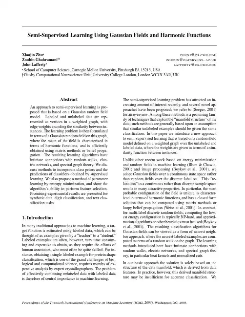
Xiaojin Zhu ZHUXJ@ Zoubin Ghahramani ZOUBIN@ John Lafferty LAFFERTY@ School of Computer Science,Carnegie Mellon University,Pittsburgh PA15213,USAGatsby Computational Neuroscience Unit,University College London,London WC1N3AR,UKAbstractAn approach to semi-supervised learning is pro-posed that is based on a Gaussian randomfieldbeled and unlabeled data are rep-resented as vertices in a weighted graph,withedge weights encoding the similarity between in-stances.The learning problem is then formulatedin terms of a Gaussian randomfield on this graph,where the mean of thefield is characterized interms of harmonic functions,and is efficientlyobtained using matrix methods or belief propa-gation.The resulting learning algorithms haveintimate connections with random walks,elec-tric networks,and spectral graph theory.We dis-cuss methods to incorporate class priors and thepredictions of classifiers obtained by supervisedlearning.We also propose a method of parameterlearning by entropy minimization,and show thealgorithm’s ability to perform feature selection.Promising experimental results are presented forsynthetic data,digit classification,and text clas-sification tasks.1.IntroductionIn many traditional approaches to machine learning,a tar-get function is estimated using labeled data,which can be thought of as examples given by a“teacher”to a“student.”Labeled examples are often,however,very time consum-ing and expensive to obtain,as they require the efforts of human annotators,who must often be quite skilled.For in-stance,obtaining a single labeled example for protein shape classification,which is one of the grand challenges of bio-logical and computational science,requires months of ex-pensive analysis by expert crystallographers.The problem of effectively combining unlabeled data with labeled data is therefore of central importance in machine learning.The semi-supervised learning problem has attracted an in-creasing amount of interest recently,and several novel ap-proaches have been proposed;we refer to(Seeger,2001) for an overview.Among these methods is a promising fam-ily of techniques that exploit the“manifold structure”of the data;such methods are generally based upon an assumption that similar unlabeled examples should be given the same classification.In this paper we introduce a new approach to semi-supervised learning that is based on a randomfield model defined on a weighted graph over the unlabeled and labeled data,where the weights are given in terms of a sim-ilarity function between instances.Unlike other recent work based on energy minimization and randomfields in machine learning(Blum&Chawla, 2001)and image processing(Boykov et al.,2001),we adopt Gaussianfields over a continuous state space rather than randomfields over the discrete label set.This“re-laxation”to a continuous rather than discrete sample space results in many attractive properties.In particular,the most probable configuration of thefield is unique,is character-ized in terms of harmonic functions,and has a closed form solution that can be computed using matrix methods or loopy belief propagation(Weiss et al.,2001).In contrast, for multi-label discrete randomfields,computing the low-est energy configuration is typically NP-hard,and approxi-mation algorithms or other heuristics must be used(Boykov et al.,2001).The resulting classification algorithms for Gaussianfields can be viewed as a form of nearest neigh-bor approach,where the nearest labeled examples are com-puted in terms of a random walk on the graph.The learning methods introduced here have intimate connections with random walks,electric networks,and spectral graph the-ory,in particular heat kernels and normalized cuts.In our basic approach the solution is solely based on the structure of the data manifold,which is derived from data features.In practice,however,this derived manifold struc-ture may be insufficient for accurate classification.WeProceedings of the Twentieth International Conference on Machine Learning(ICML-2003),Washington DC,2003.Figure1.The randomfields used in this work are constructed on labeled and unlabeled examples.We form a graph with weighted edges between instances(in this case scanned digits),with labeled data items appearing as special“boundary”points,and unlabeled points as“interior”points.We consider Gaussian randomfields on this graph.show how the extra evidence of class priors can help classi-fication in Section4.Alternatively,we may combine exter-nal classifiers using vertex weights or“assignment costs,”as described in Section5.Encouraging experimental re-sults for synthetic data,digit classification,and text clas-sification tasks are presented in Section7.One difficulty with the randomfield approach is that the right choice of graph is often not entirely clear,and it may be desirable to learn it from data.In Section6we propose a method for learning these weights by entropy minimization,and show the algorithm’s ability to perform feature selection to better characterize the data manifold.2.Basic FrameworkWe suppose there are labeled points, and unlabeled points;typically. Let be the total number of data points.To be-gin,we assume the labels are binary:.Consider a connected graph with nodes correspond-ing to the data points,with nodes corre-sponding to the labeled points with labels,and nodes corresponding to the unla-beled points.Our task is to assign labels to nodes.We assume an symmetric weight matrix on the edges of the graph is given.For example,when,the weight matrix can be(2)To assign a probability distribution on functions,we form the Gaussianfieldfor(3) which is consistent with our prior notion of smoothness of with respect to the graph.Expressed slightly differently, ,where.Because of the maximum principle of harmonic functions(Doyle&Snell,1984),is unique and is either a constant or it satisfiesfor.To compute the harmonic solution explicitly in terms of matrix operations,we split the weight matrix(and sim-ilarly)into4blocks after the th row and column:(4) Letting where denotes the values on the un-labeled data points,the harmonic solution subject to is given by(5)Figure2.Demonstration of harmonic energy minimization on twosynthetic rge symbols indicate labeled data,otherpoints are unlabeled.In this paper we focus on the above harmonic function as abasis for semi-supervised classification.However,we em-phasize that the Gaussian randomfield model from which this function is derived provides the learning frameworkwith a consistent probabilistic semantics.In the following,we refer to the procedure described aboveas harmonic energy minimization,to underscore the har-monic property(3)as well as the objective function being minimized.Figure2demonstrates the use of harmonic en-ergy minimization on two synthetic datasets.The leftfigure shows that the data has three bands,with,, and;the rightfigure shows two spirals,with,,and.Here we see harmonic energy minimization clearly follows the structure of data, while obviously methods such as kNN would fail to do so.3.Interpretation and ConnectionsAs outlined briefly in this section,the basic framework pre-sented in the previous section can be viewed in several fun-damentally different ways,and these different viewpoints provide a rich and complementary set of techniques for rea-soning about this approach to the semi-supervised learning problem.3.1.Random Walks and Electric NetworksImagine a particle walking along the graph.Starting from an unlabeled node,it moves to a node with proba-bility after one step.The walk continues until the par-ticle hits a labeled node.Then is the probability that the particle,starting from node,hits a labeled node with label1.Here the labeled data is viewed as an“absorbing boundary”for the random walk.This view of the harmonic solution indicates that it is closely related to the random walk approach of Szummer and Jaakkola(2001),however there are two major differ-ences.First,wefix the value of on the labeled points, and second,our solution is an equilibrium state,expressed in terms of a hitting time,while in(Szummer&Jaakkola,2001)the walk crucially depends on the time parameter. We will return to this point when discussing heat kernels. An electrical network interpretation is given in(Doyle& Snell,1984).Imagine the edges of to be resistors with conductance.We connect nodes labeled to a positive voltage source,and points labeled to ground.Thenis the voltage in the resulting electric network on each of the unlabeled nodes.Furthermore minimizes the energy dissipation of the electric network for the given.The harmonic property here follows from Kirchoff’s and Ohm’s laws,and the maximum principle then shows that this is precisely the same solution obtained in(5).3.2.Graph KernelsThe solution can be viewed from the viewpoint of spec-tral graph theory.The heat kernel with time parameter on the graph is defined as.Here is the solution to the heat equation on the graph with initial conditions being a point source at at time.Kondor and Lafferty(2002)propose this as an appropriate kernel for machine learning with categorical data.When used in a kernel method such as a support vector machine,the kernel classifier can be viewed as a solution to the heat equation with initial heat sourceson the labeled data.The time parameter must,however, be chosen using an auxiliary technique,for example cross-validation.Our algorithm uses a different approach which is indepen-dent of,the diffusion time.Let be the lower right submatrix of.Since,it is the Laplacian restricted to the unlabeled nodes in.Consider the heat kernel on this submatrix:.Then describes heat diffusion on the unlabeled subgraph with Dirichlet boundary conditions on the labeled nodes.The Green’s function is the inverse operator of the restricted Laplacian,,which can be expressed in terms of the integral over time of the heat kernel:(6) The harmonic solution(5)can then be written asor(7)Expression(7)shows that this approach can be viewed as a kernel classifier with the kernel and a specific form of kernel machine.(See also(Chung&Yau,2000),where a normalized Laplacian is used instead of the combinatorial Laplacian.)From(6)we also see that the spectrum of is ,where is the spectrum of.This indicates a connection to the work of Chapelle et al.(2002),who ma-nipulate the eigenvalues of the Laplacian to create variouskernels.A related approach is given by Belkin and Niyogi (2002),who propose to regularize functions on by select-ing the top normalized eigenvectors of corresponding to the smallest eigenvalues,thus obtaining the bestfit toin the least squares sense.We remark that ourfits the labeled data exactly,while the order approximation may not.3.3.Spectral Clustering and Graph MincutsThe normalized cut approach of Shi and Malik(2000)has as its objective function the minimization of the Raleigh quotient(8)subject to the constraint.The solution is the second smallest eigenvector of the generalized eigenvalue problem .Yu and Shi(2001)add a grouping bias to the normalized cut to specify which points should be in the same group.Since labeled data can be encoded into such pairwise grouping constraints,this technique can be applied to semi-supervised learning as well.In general, when is close to block diagonal,it can be shown that data points are tightly clustered in the eigenspace spanned by thefirst few eigenvectors of(Ng et al.,2001a;Meila &Shi,2001),leading to various spectral clustering algo-rithms.Perhaps the most interesting and substantial connection to the methods we propose here is the graph mincut approach proposed by Blum and Chawla(2001).The starting point for this work is also a weighted graph,but the semi-supervised learning problem is cast as one offinding a minimum-cut,where negative labeled data is connected (with large weight)to a special source node,and positive labeled data is connected to a special sink node.A mini-mum-cut,which is not necessarily unique,minimizes the objective function,and label0other-wise.We call this rule the harmonic threshold(abbreviated “thresh”below).In terms of the random walk interpreta-tion,ifmakes sense.If there is reason to doubt this assumption,it would be reasonable to attach dongles to labeled nodes as well,and to move the labels to these new nodes.6.Learning the Weight MatrixPreviously we assumed that the weight matrix is given andfixed.In this section,we investigate learning weight functions of the form given by equation(1).We will learn the’s from both labeled and unlabeled data;this will be shown to be useful as a feature selection mechanism which better aligns the graph structure with the data.The usual parameter learning criterion is to maximize the likelihood of labeled data.However,the likelihood crite-rion is not appropriate in this case because the values for labeled data arefixed during training,and moreover likeli-hood doesn’t make sense for the unlabeled data because we do not have a generative model.We propose instead to use average label entropy as a heuristic criterion for parameter learning.The average label entropy of thefield is defined as(13) using the fact that.Both and are sub-matrices of.In the above derivation we use as label probabilities di-rectly;that is,class.If we incorpo-rate class prior information,or combine harmonic energy minimization with other classifiers,it makes sense to min-imize entropy on the combined probabilities.For instance, if we incorporate a class prior using CMN,the probability is given bylabeled set size a c c u r a c yFigure 3.Harmonic energy minimization on digits “1”vs.“2”(left)and on all 10digits (middle)and combining voted-perceptron with harmonic energy minimization on odd vs.even digits (right)Figure 4.Harmonic energy minimization on PC vs.MAC (left),baseball vs.hockey (middle),and MS-Windows vs.MAC (right)10trials.In each trial we randomly sample labeled data from the entire dataset,and use the rest of the images as unlabeled data.If any class is absent from the sampled la-beled set,we redo the sampling.For methods that incorpo-rate class priors ,we estimate from the labeled set with Laplace (“add one”)smoothing.We consider the binary problem of classifying digits “1”vs.“2,”with 1100images in each class.We report aver-age accuracy of the following methods on unlabeled data:thresh,CMN,1NN,and a radial basis function classifier (RBF)which classifies to class 1iff .RBF and 1NN are used simply as baselines.The results are shown in Figure 3.Clearly thresh performs poorly,because the values of are generally close to 1,so the major-ity of examples are classified as digit “1”.This shows the inadequacy of the weight function (1)based on pixel-wise Euclidean distance.However the relative rankings ofare useful,and when coupled with class prior information significantly improved accuracy is obtained.The greatest improvement is achieved by the simple method CMN.We could also have adjusted the decision threshold on thresh’s solution ,so that the class proportion fits the prior .This method is inferior to CMN due to the error in estimating ,and it is not shown in the plot.These same observations are also true for the experiments we performed on several other binary digit classification problems.We also consider the 10-way problem of classifying digits “0”through ’9’.We report the results on a dataset with in-tentionally unbalanced class sizes,with 455,213,129,100,754,970,275,585,166,353examples per class,respec-tively (noting that the results on a balanced dataset are sim-ilar).We report the average accuracy of thresh,CMN,RBF,and 1NN.These methods can handle multi-way classifica-tion directly,or with slight modification in a one-against-all fashion.As the results in Figure 3show,CMN again im-proves performance by incorporating class priors.Next we report the results of document categorization ex-periments using the 20newsgroups dataset.We pick three binary problems:PC (number of documents:982)vs.MAC (961),MS-Windows (958)vs.MAC,and base-ball (994)vs.hockey (999).Each document is minimally processed into a “tf.idf”vector,without applying header re-moval,frequency cutoff,stemming,or a stopword list.Two documents are connected by an edge if is among ’s 10nearest neighbors or if is among ’s 10nearest neigh-bors,as measured by cosine similarity.We use the follow-ing weight function on the edges:(16)We use one-nearest neighbor and the voted perceptron al-gorithm (Freund &Schapire,1999)(10epochs with a lin-ear kernel)as baselines–our results with support vector ma-chines are comparable.The results are shown in Figure 4.As before,each point is the average of10random tri-als.For this data,harmonic energy minimization performsmuch better than the baselines.The improvement from the class prior,however,is less significant.An explanation for why this approach to semi-supervised learning is so effec-tive on the newsgroups data may lie in the common use of quotations within a topic thread:document quotes partof document,quotes part of,and so on.Thus, although documents far apart in the thread may be quite different,they are linked by edges in the graphical repre-sentation of the data,and these links are exploited by the learning algorithm.7.1.Incorporating External ClassifiersWe use the voted-perceptron as our external classifier.For each random trial,we train a voted-perceptron on the la-beled set,and apply it to the unlabeled set.We then use the 0/1hard labels for dongle values,and perform harmonic energy minimization with(10).We use.We evaluate on the artificial but difficult binary problem of classifying odd digits vs.even digits;that is,we group “1,3,5,7,9”and“2,4,6,8,0”into two classes.There are400 images per digit.We use second order polynomial kernel in the voted-perceptron,and train for10epochs.Figure3 shows the results.The accuracy of the voted-perceptron on unlabeled data,averaged over trials,is marked VP in the plot.Independently,we run thresh and CMN.Next we combine thresh with the voted-perceptron,and the result is marked thresh+VP.Finally,we perform class mass nor-malization on the combined result and get CMN+VP.The combination results in higher accuracy than either method alone,suggesting there is complementary information used by each.7.2.Learning the Weight MatrixTo demonstrate the effects of estimating,results on a toy dataset are shown in Figure5.The upper grid is slightly tighter than the lower grid,and they are connected by a few data points.There are two labeled examples,marked with large symbols.We learn the optimal length scales for this dataset by minimizing entropy on unlabeled data.To simplify the problem,wefirst tie the length scales in the two dimensions,so there is only a single parameter to learn.As noted earlier,without smoothing,the entropy approaches the minimum at0as.Under such con-ditions,the results of harmonic energy minimization are usually undesirable,and for this dataset the tighter grid “invades”the sparser one as shown in Figure5(a).With smoothing,the“nuisance minimum”at0gradually disap-pears as the smoothing factor grows,as shown in FigureFigure5.The effect of parameter on harmonic energy mini-mization.(a)If unsmoothed,as,and the algorithm performs poorly.(b)Result at optimal,smoothed with(c)Smoothing helps to remove the entropy minimum. 5(c).When we set,the minimum entropy is0.898 bits at.Harmonic energy minimization under this length scale is shown in Figure5(b),which is able to dis-tinguish the structure of the two grids.If we allow a separate for each dimension,parameter learning is more dramatic.With the same smoothing of ,keeps growing towards infinity(we usefor computation)while stabilizes at0.65, and we reach a minimum entropy of0.619bits.In this case is legitimate;it means that the learning al-gorithm has identified the-direction as irrelevant,based on both the labeled and unlabeled data.Harmonic energy minimization under these parameters gives the same clas-sification as shown in Figure5(b).Next we learn’s for all256dimensions on the“1”vs.“2”digits dataset.For this problem we minimize the entropy with CMN probabilities(15).We randomly pick a split of 92labeled and2108unlabeled examples,and start with all dimensions sharing the same as in previous ex-periments.Then we compute the derivatives of for each dimension separately,and perform gradient descent to min-imize the entropy.The result is shown in Table1.As entropy decreases,the accuracy of CMN and thresh both increase.The learned’s shown in the rightmost plot of Figure6range from181(black)to465(white).A small (black)indicates that the weight is more sensitive to varia-tions in that dimension,while the opposite is true for large (white).We can discern the shapes of a black“1”and a white“2”in thisfigure;that is,the learned parametersCMNstart97.250.73%0.654298.020.39%Table1.Entropy of CMN and accuracies before and after learning ’s on the“1”vs.“2”dataset.Figure6.Learned’s for“1”vs.“2”dataset.From left to right: average“1”,average“2”,initial’s,learned’s.exaggerate variations within class“1”while suppressing variations within class“2”.We have observed that with the default parameters,class“1”has much less variation than class“2”;thus,the learned parameters are,in effect, compensating for the relative tightness of the two classes in feature space.8.ConclusionWe have introduced an approach to semi-supervised learn-ing based on a Gaussian randomfield model defined with respect to a weighted graph representing labeled and unla-beled data.Promising experimental results have been pre-sented for text and digit classification,demonstrating that the framework has the potential to effectively exploit the structure of unlabeled data to improve classification accu-racy.The underlying randomfield gives a coherent proba-bilistic semantics to our approach,but this paper has con-centrated on the use of only the mean of thefield,which is characterized in terms of harmonic functions and spectral graph theory.The fully probabilistic framework is closely related to Gaussian process classification,and this connec-tion suggests principled ways of incorporating class priors and learning hyperparameters;in particular,it is natural to apply evidence maximization or the generalization er-ror bounds that have been studied for Gaussian processes (Seeger,2002).Our work in this direction will be reported in a future publication.ReferencesBelkin,M.,&Niyogi,P.(2002).Using manifold structure for partially labelled classification.Advances in Neural Information Processing Systems,15.Blum,A.,&Chawla,S.(2001).Learning from labeled and unlabeled data using graph mincuts.Proc.18th Interna-tional Conf.on Machine Learning.Boykov,Y.,Veksler,O.,&Zabih,R.(2001).Fast approx-imate energy minimization via graph cuts.IEEE Trans. on Pattern Analysis and Machine Intelligence,23. Chapelle,O.,Weston,J.,&Sch¨o lkopf,B.(2002).Cluster kernels for semi-supervised learning.Advances in Neu-ral Information Processing Systems,15.Chung,F.,&Yau,S.(2000).Discrete Green’s functions. Journal of Combinatorial Theory(A)(pp.191–214). Doyle,P.,&Snell,J.(1984).Random walks and electric networks.Mathematical Assoc.of America. Freund,Y.,&Schapire,R.E.(1999).Large margin classi-fication using the perceptron algorithm.Machine Learn-ing,37(3),277–296.Hull,J.J.(1994).A database for handwritten text recog-nition research.IEEE Transactions on Pattern Analysis and Machine Intelligence,16.Kondor,R.I.,&Lafferty,J.(2002).Diffusion kernels on graphs and other discrete input spaces.Proc.19th Inter-national Conf.on Machine Learning.Le Cun,Y.,Boser, B.,Denker,J.S.,Henderson, D., Howard,R.E.,Howard,W.,&Jackel,L.D.(1990). Handwritten digit recognition with a back-propagation network.Advances in Neural Information Processing Systems,2.Meila,M.,&Shi,J.(2001).A random walks view of spec-tral segmentation.AISTATS.Ng,A.,Jordan,M.,&Weiss,Y.(2001a).On spectral clus-tering:Analysis and an algorithm.Advances in Neural Information Processing Systems,14.Ng,A.Y.,Zheng,A.X.,&Jordan,M.I.(2001b).Link analysis,eigenvectors and stability.International Joint Conference on Artificial Intelligence(IJCAI). Seeger,M.(2001).Learning with labeled and unlabeled data(Technical Report).University of Edinburgh. Seeger,M.(2002).PAC-Bayesian generalization error bounds for Gaussian process classification.Journal of Machine Learning Research,3,233–269.Shi,J.,&Malik,J.(2000).Normalized cuts and image segmentation.IEEE Transactions on Pattern Analysis and Machine Intelligence,22,888–905.Szummer,M.,&Jaakkola,T.(2001).Partially labeled clas-sification with Markov random walks.Advances in Neu-ral Information Processing Systems,14.Weiss,Y.,,&Freeman,W.T.(2001).Correctness of belief propagation in Gaussian graphical models of arbitrary topology.Neural Computation,13,2173–2200.Yu,S.X.,&Shi,J.(2001).Grouping with bias.Advances in Neural Information Processing Systems,14.。

机器学习与人工智能领域中常用的英语词汇1.General Concepts (基础概念)•Artificial Intelligence (AI) - 人工智能1)Artificial Intelligence (AI) - 人工智能2)Machine Learning (ML) - 机器学习3)Deep Learning (DL) - 深度学习4)Neural Network - 神经网络5)Natural Language Processing (NLP) - 自然语言处理6)Computer Vision - 计算机视觉7)Robotics - 机器人技术8)Speech Recognition - 语音识别9)Expert Systems - 专家系统10)Knowledge Representation - 知识表示11)Pattern Recognition - 模式识别12)Cognitive Computing - 认知计算13)Autonomous Systems - 自主系统14)Human-Machine Interaction - 人机交互15)Intelligent Agents - 智能代理16)Machine Translation - 机器翻译17)Swarm Intelligence - 群体智能18)Genetic Algorithms - 遗传算法19)Fuzzy Logic - 模糊逻辑20)Reinforcement Learning - 强化学习•Machine Learning (ML) - 机器学习1)Machine Learning (ML) - 机器学习2)Artificial Neural Network - 人工神经网络3)Deep Learning - 深度学习4)Supervised Learning - 有监督学习5)Unsupervised Learning - 无监督学习6)Reinforcement Learning - 强化学习7)Semi-Supervised Learning - 半监督学习8)Training Data - 训练数据9)Test Data - 测试数据10)Validation Data - 验证数据11)Feature - 特征12)Label - 标签13)Model - 模型14)Algorithm - 算法15)Regression - 回归16)Classification - 分类17)Clustering - 聚类18)Dimensionality Reduction - 降维19)Overfitting - 过拟合20)Underfitting - 欠拟合•Deep Learning (DL) - 深度学习1)Deep Learning - 深度学习2)Neural Network - 神经网络3)Artificial Neural Network (ANN) - 人工神经网络4)Convolutional Neural Network (CNN) - 卷积神经网络5)Recurrent Neural Network (RNN) - 循环神经网络6)Long Short-Term Memory (LSTM) - 长短期记忆网络7)Gated Recurrent Unit (GRU) - 门控循环单元8)Autoencoder - 自编码器9)Generative Adversarial Network (GAN) - 生成对抗网络10)Transfer Learning - 迁移学习11)Pre-trained Model - 预训练模型12)Fine-tuning - 微调13)Feature Extraction - 特征提取14)Activation Function - 激活函数15)Loss Function - 损失函数16)Gradient Descent - 梯度下降17)Backpropagation - 反向传播18)Epoch - 训练周期19)Batch Size - 批量大小20)Dropout - 丢弃法•Neural Network - 神经网络1)Neural Network - 神经网络2)Artificial Neural Network (ANN) - 人工神经网络3)Deep Neural Network (DNN) - 深度神经网络4)Convolutional Neural Network (CNN) - 卷积神经网络5)Recurrent Neural Network (RNN) - 循环神经网络6)Long Short-Term Memory (LSTM) - 长短期记忆网络7)Gated Recurrent Unit (GRU) - 门控循环单元8)Feedforward Neural Network - 前馈神经网络9)Multi-layer Perceptron (MLP) - 多层感知器10)Radial Basis Function Network (RBFN) - 径向基函数网络11)Hopfield Network - 霍普菲尔德网络12)Boltzmann Machine - 玻尔兹曼机13)Autoencoder - 自编码器14)Spiking Neural Network (SNN) - 脉冲神经网络15)Self-organizing Map (SOM) - 自组织映射16)Restricted Boltzmann Machine (RBM) - 受限玻尔兹曼机17)Hebbian Learning - 海比安学习18)Competitive Learning - 竞争学习19)Neuroevolutionary - 神经进化20)Neuron - 神经元•Algorithm - 算法1)Algorithm - 算法2)Supervised Learning Algorithm - 有监督学习算法3)Unsupervised Learning Algorithm - 无监督学习算法4)Reinforcement Learning Algorithm - 强化学习算法5)Classification Algorithm - 分类算法6)Regression Algorithm - 回归算法7)Clustering Algorithm - 聚类算法8)Dimensionality Reduction Algorithm - 降维算法9)Decision Tree Algorithm - 决策树算法10)Random Forest Algorithm - 随机森林算法11)Support Vector Machine (SVM) Algorithm - 支持向量机算法12)K-Nearest Neighbors (KNN) Algorithm - K近邻算法13)Naive Bayes Algorithm - 朴素贝叶斯算法14)Gradient Descent Algorithm - 梯度下降算法15)Genetic Algorithm - 遗传算法16)Neural Network Algorithm - 神经网络算法17)Deep Learning Algorithm - 深度学习算法18)Ensemble Learning Algorithm - 集成学习算法19)Reinforcement Learning Algorithm - 强化学习算法20)Metaheuristic Algorithm - 元启发式算法•Model - 模型1)Model - 模型2)Machine Learning Model - 机器学习模型3)Artificial Intelligence Model - 人工智能模型4)Predictive Model - 预测模型5)Classification Model - 分类模型6)Regression Model - 回归模型7)Generative Model - 生成模型8)Discriminative Model - 判别模型9)Probabilistic Model - 概率模型10)Statistical Model - 统计模型11)Neural Network Model - 神经网络模型12)Deep Learning Model - 深度学习模型13)Ensemble Model - 集成模型14)Reinforcement Learning Model - 强化学习模型15)Support Vector Machine (SVM) Model - 支持向量机模型16)Decision Tree Model - 决策树模型17)Random Forest Model - 随机森林模型18)Naive Bayes Model - 朴素贝叶斯模型19)Autoencoder Model - 自编码器模型20)Convolutional Neural Network (CNN) Model - 卷积神经网络模型•Dataset - 数据集1)Dataset - 数据集2)Training Dataset - 训练数据集3)Test Dataset - 测试数据集4)Validation Dataset - 验证数据集5)Balanced Dataset - 平衡数据集6)Imbalanced Dataset - 不平衡数据集7)Synthetic Dataset - 合成数据集8)Benchmark Dataset - 基准数据集9)Open Dataset - 开放数据集10)Labeled Dataset - 标记数据集11)Unlabeled Dataset - 未标记数据集12)Semi-Supervised Dataset - 半监督数据集13)Multiclass Dataset - 多分类数据集14)Feature Set - 特征集15)Data Augmentation - 数据增强16)Data Preprocessing - 数据预处理17)Missing Data - 缺失数据18)Outlier Detection - 异常值检测19)Data Imputation - 数据插补20)Metadata - 元数据•Training - 训练1)Training - 训练2)Training Data - 训练数据3)Training Phase - 训练阶段4)Training Set - 训练集5)Training Examples - 训练样本6)Training Instance - 训练实例7)Training Algorithm - 训练算法8)Training Model - 训练模型9)Training Process - 训练过程10)Training Loss - 训练损失11)Training Epoch - 训练周期12)Training Batch - 训练批次13)Online Training - 在线训练14)Offline Training - 离线训练15)Continuous Training - 连续训练16)Transfer Learning - 迁移学习17)Fine-Tuning - 微调18)Curriculum Learning - 课程学习19)Self-Supervised Learning - 自监督学习20)Active Learning - 主动学习•Testing - 测试1)Testing - 测试2)Test Data - 测试数据3)Test Set - 测试集4)Test Examples - 测试样本5)Test Instance - 测试实例6)Test Phase - 测试阶段7)Test Accuracy - 测试准确率8)Test Loss - 测试损失9)Test Error - 测试错误10)Test Metrics - 测试指标11)Test Suite - 测试套件12)Test Case - 测试用例13)Test Coverage - 测试覆盖率14)Cross-Validation - 交叉验证15)Holdout Validation - 留出验证16)K-Fold Cross-Validation - K折交叉验证17)Stratified Cross-Validation - 分层交叉验证18)Test Driven Development (TDD) - 测试驱动开发19)A/B Testing - A/B 测试20)Model Evaluation - 模型评估•Validation - 验证1)Validation - 验证2)Validation Data - 验证数据3)Validation Set - 验证集4)Validation Examples - 验证样本5)Validation Instance - 验证实例6)Validation Phase - 验证阶段7)Validation Accuracy - 验证准确率8)Validation Loss - 验证损失9)Validation Error - 验证错误10)Validation Metrics - 验证指标11)Cross-Validation - 交叉验证12)Holdout Validation - 留出验证13)K-Fold Cross-Validation - K折交叉验证14)Stratified Cross-Validation - 分层交叉验证15)Leave-One-Out Cross-Validation - 留一法交叉验证16)Validation Curve - 验证曲线17)Hyperparameter Validation - 超参数验证18)Model Validation - 模型验证19)Early Stopping - 提前停止20)Validation Strategy - 验证策略•Supervised Learning - 有监督学习1)Supervised Learning - 有监督学习2)Label - 标签3)Feature - 特征4)Target - 目标5)Training Labels - 训练标签6)Training Features - 训练特征7)Training Targets - 训练目标8)Training Examples - 训练样本9)Training Instance - 训练实例10)Regression - 回归11)Classification - 分类12)Predictor - 预测器13)Regression Model - 回归模型14)Classifier - 分类器15)Decision Tree - 决策树16)Support Vector Machine (SVM) - 支持向量机17)Neural Network - 神经网络18)Feature Engineering - 特征工程19)Model Evaluation - 模型评估20)Overfitting - 过拟合21)Underfitting - 欠拟合22)Bias-Variance Tradeoff - 偏差-方差权衡•Unsupervised Learning - 无监督学习1)Unsupervised Learning - 无监督学习2)Clustering - 聚类3)Dimensionality Reduction - 降维4)Anomaly Detection - 异常检测5)Association Rule Learning - 关联规则学习6)Feature Extraction - 特征提取7)Feature Selection - 特征选择8)K-Means - K均值9)Hierarchical Clustering - 层次聚类10)Density-Based Clustering - 基于密度的聚类11)Principal Component Analysis (PCA) - 主成分分析12)Independent Component Analysis (ICA) - 独立成分分析13)T-distributed Stochastic Neighbor Embedding (t-SNE) - t分布随机邻居嵌入14)Gaussian Mixture Model (GMM) - 高斯混合模型15)Self-Organizing Maps (SOM) - 自组织映射16)Autoencoder - 自动编码器17)Latent Variable - 潜变量18)Data Preprocessing - 数据预处理19)Outlier Detection - 异常值检测20)Clustering Algorithm - 聚类算法•Reinforcement Learning - 强化学习1)Reinforcement Learning - 强化学习2)Agent - 代理3)Environment - 环境4)State - 状态5)Action - 动作6)Reward - 奖励7)Policy - 策略8)Value Function - 值函数9)Q-Learning - Q学习10)Deep Q-Network (DQN) - 深度Q网络11)Policy Gradient - 策略梯度12)Actor-Critic - 演员-评论家13)Exploration - 探索14)Exploitation - 开发15)Temporal Difference (TD) - 时间差分16)Markov Decision Process (MDP) - 马尔可夫决策过程17)State-Action-Reward-State-Action (SARSA) - 状态-动作-奖励-状态-动作18)Policy Iteration - 策略迭代19)Value Iteration - 值迭代20)Monte Carlo Methods - 蒙特卡洛方法•Semi-Supervised Learning - 半监督学习1)Semi-Supervised Learning - 半监督学习2)Labeled Data - 有标签数据3)Unlabeled Data - 无标签数据4)Label Propagation - 标签传播5)Self-Training - 自训练6)Co-Training - 协同训练7)Transudative Learning - 传导学习8)Inductive Learning - 归纳学习9)Manifold Regularization - 流形正则化10)Graph-based Methods - 基于图的方法11)Cluster Assumption - 聚类假设12)Low-Density Separation - 低密度分离13)Semi-Supervised Support Vector Machines (S3VM) - 半监督支持向量机14)Expectation-Maximization (EM) - 期望最大化15)Co-EM - 协同期望最大化16)Entropy-Regularized EM - 熵正则化EM17)Mean Teacher - 平均教师18)Virtual Adversarial Training - 虚拟对抗训练19)Tri-training - 三重训练20)Mix Match - 混合匹配•Feature - 特征1)Feature - 特征2)Feature Engineering - 特征工程3)Feature Extraction - 特征提取4)Feature Selection - 特征选择5)Input Features - 输入特征6)Output Features - 输出特征7)Feature Vector - 特征向量8)Feature Space - 特征空间9)Feature Representation - 特征表示10)Feature Transformation - 特征转换11)Feature Importance - 特征重要性12)Feature Scaling - 特征缩放13)Feature Normalization - 特征归一化14)Feature Encoding - 特征编码15)Feature Fusion - 特征融合16)Feature Dimensionality Reduction - 特征维度减少17)Continuous Feature - 连续特征18)Categorical Feature - 分类特征19)Nominal Feature - 名义特征20)Ordinal Feature - 有序特征•Label - 标签1)Label - 标签2)Labeling - 标注3)Ground Truth - 地面真值4)Class Label - 类别标签5)Target Variable - 目标变量6)Labeling Scheme - 标注方案7)Multi-class Labeling - 多类别标注8)Binary Labeling - 二分类标注9)Label Noise - 标签噪声10)Labeling Error - 标注错误11)Label Propagation - 标签传播12)Unlabeled Data - 无标签数据13)Labeled Data - 有标签数据14)Semi-supervised Learning - 半监督学习15)Active Learning - 主动学习16)Weakly Supervised Learning - 弱监督学习17)Noisy Label Learning - 噪声标签学习18)Self-training - 自训练19)Crowdsourcing Labeling - 众包标注20)Label Smoothing - 标签平滑化•Prediction - 预测1)Prediction - 预测2)Forecasting - 预测3)Regression - 回归4)Classification - 分类5)Time Series Prediction - 时间序列预测6)Forecast Accuracy - 预测准确性7)Predictive Modeling - 预测建模8)Predictive Analytics - 预测分析9)Forecasting Method - 预测方法10)Predictive Performance - 预测性能11)Predictive Power - 预测能力12)Prediction Error - 预测误差13)Prediction Interval - 预测区间14)Prediction Model - 预测模型15)Predictive Uncertainty - 预测不确定性16)Forecast Horizon - 预测时间跨度17)Predictive Maintenance - 预测性维护18)Predictive Policing - 预测式警务19)Predictive Healthcare - 预测性医疗20)Predictive Maintenance - 预测性维护•Classification - 分类1)Classification - 分类2)Classifier - 分类器3)Class - 类别4)Classify - 对数据进行分类5)Class Label - 类别标签6)Binary Classification - 二元分类7)Multiclass Classification - 多类分类8)Class Probability - 类别概率9)Decision Boundary - 决策边界10)Decision Tree - 决策树11)Support Vector Machine (SVM) - 支持向量机12)K-Nearest Neighbors (KNN) - K最近邻算法13)Naive Bayes - 朴素贝叶斯14)Logistic Regression - 逻辑回归15)Random Forest - 随机森林16)Neural Network - 神经网络17)SoftMax Function - SoftMax函数18)One-vs-All (One-vs-Rest) - 一对多(一对剩余)19)Ensemble Learning - 集成学习20)Confusion Matrix - 混淆矩阵•Regression - 回归1)Regression Analysis - 回归分析2)Linear Regression - 线性回归3)Multiple Regression - 多元回归4)Polynomial Regression - 多项式回归5)Logistic Regression - 逻辑回归6)Ridge Regression - 岭回归7)Lasso Regression - Lasso回归8)Elastic Net Regression - 弹性网络回归9)Regression Coefficients - 回归系数10)Residuals - 残差11)Ordinary Least Squares (OLS) - 普通最小二乘法12)Ridge Regression Coefficient - 岭回归系数13)Lasso Regression Coefficient - Lasso回归系数14)Elastic Net Regression Coefficient - 弹性网络回归系数15)Regression Line - 回归线16)Prediction Error - 预测误差17)Regression Model - 回归模型18)Nonlinear Regression - 非线性回归19)Generalized Linear Models (GLM) - 广义线性模型20)Coefficient of Determination (R-squared) - 决定系数21)F-test - F检验22)Homoscedasticity - 同方差性23)Heteroscedasticity - 异方差性24)Autocorrelation - 自相关25)Multicollinearity - 多重共线性26)Outliers - 异常值27)Cross-validation - 交叉验证28)Feature Selection - 特征选择29)Feature Engineering - 特征工程30)Regularization - 正则化2.Neural Networks and Deep Learning (神经网络与深度学习)•Convolutional Neural Network (CNN) - 卷积神经网络1)Convolutional Neural Network (CNN) - 卷积神经网络2)Convolution Layer - 卷积层3)Feature Map - 特征图4)Convolution Operation - 卷积操作5)Stride - 步幅6)Padding - 填充7)Pooling Layer - 池化层8)Max Pooling - 最大池化9)Average Pooling - 平均池化10)Fully Connected Layer - 全连接层11)Activation Function - 激活函数12)Rectified Linear Unit (ReLU) - 线性修正单元13)Dropout - 随机失活14)Batch Normalization - 批量归一化15)Transfer Learning - 迁移学习16)Fine-Tuning - 微调17)Image Classification - 图像分类18)Object Detection - 物体检测19)Semantic Segmentation - 语义分割20)Instance Segmentation - 实例分割21)Generative Adversarial Network (GAN) - 生成对抗网络22)Image Generation - 图像生成23)Style Transfer - 风格迁移24)Convolutional Autoencoder - 卷积自编码器25)Recurrent Neural Network (RNN) - 循环神经网络•Recurrent Neural Network (RNN) - 循环神经网络1)Recurrent Neural Network (RNN) - 循环神经网络2)Long Short-Term Memory (LSTM) - 长短期记忆网络3)Gated Recurrent Unit (GRU) - 门控循环单元4)Sequence Modeling - 序列建模5)Time Series Prediction - 时间序列预测6)Natural Language Processing (NLP) - 自然语言处理7)Text Generation - 文本生成8)Sentiment Analysis - 情感分析9)Named Entity Recognition (NER) - 命名实体识别10)Part-of-Speech Tagging (POS Tagging) - 词性标注11)Sequence-to-Sequence (Seq2Seq) - 序列到序列12)Attention Mechanism - 注意力机制13)Encoder-Decoder Architecture - 编码器-解码器架构14)Bidirectional RNN - 双向循环神经网络15)Teacher Forcing - 强制教师法16)Backpropagation Through Time (BPTT) - 通过时间的反向传播17)Vanishing Gradient Problem - 梯度消失问题18)Exploding Gradient Problem - 梯度爆炸问题19)Language Modeling - 语言建模20)Speech Recognition - 语音识别•Long Short-Term Memory (LSTM) - 长短期记忆网络1)Long Short-Term Memory (LSTM) - 长短期记忆网络2)Cell State - 细胞状态3)Hidden State - 隐藏状态4)Forget Gate - 遗忘门5)Input Gate - 输入门6)Output Gate - 输出门7)Peephole Connections - 窥视孔连接8)Gated Recurrent Unit (GRU) - 门控循环单元9)Vanishing Gradient Problem - 梯度消失问题10)Exploding Gradient Problem - 梯度爆炸问题11)Sequence Modeling - 序列建模12)Time Series Prediction - 时间序列预测13)Natural Language Processing (NLP) - 自然语言处理14)Text Generation - 文本生成15)Sentiment Analysis - 情感分析16)Named Entity Recognition (NER) - 命名实体识别17)Part-of-Speech Tagging (POS Tagging) - 词性标注18)Attention Mechanism - 注意力机制19)Encoder-Decoder Architecture - 编码器-解码器架构20)Bidirectional LSTM - 双向长短期记忆网络•Attention Mechanism - 注意力机制1)Attention Mechanism - 注意力机制2)Self-Attention - 自注意力3)Multi-Head Attention - 多头注意力4)Transformer - 变换器5)Query - 查询6)Key - 键7)Value - 值8)Query-Value Attention - 查询-值注意力9)Dot-Product Attention - 点积注意力10)Scaled Dot-Product Attention - 缩放点积注意力11)Additive Attention - 加性注意力12)Context Vector - 上下文向量13)Attention Score - 注意力分数14)SoftMax Function - SoftMax函数15)Attention Weight - 注意力权重16)Global Attention - 全局注意力17)Local Attention - 局部注意力18)Positional Encoding - 位置编码19)Encoder-Decoder Attention - 编码器-解码器注意力20)Cross-Modal Attention - 跨模态注意力•Generative Adversarial Network (GAN) - 生成对抗网络1)Generative Adversarial Network (GAN) - 生成对抗网络2)Generator - 生成器3)Discriminator - 判别器4)Adversarial Training - 对抗训练5)Minimax Game - 极小极大博弈6)Nash Equilibrium - 纳什均衡7)Mode Collapse - 模式崩溃8)Training Stability - 训练稳定性9)Loss Function - 损失函数10)Discriminative Loss - 判别损失11)Generative Loss - 生成损失12)Wasserstein GAN (WGAN) - Wasserstein GAN（WGAN）13)Deep Convolutional GAN (DCGAN) - 深度卷积生成对抗网络（DCGAN）14)Conditional GAN (c GAN) - 条件生成对抗网络（c GAN）15)Style GAN - 风格生成对抗网络16)Cycle GAN - 循环生成对抗网络17)Progressive Growing GAN (PGGAN) - 渐进式增长生成对抗网络（PGGAN）18)Self-Attention GAN (SAGAN) - 自注意力生成对抗网络（SAGAN）19)Big GAN - 大规模生成对抗网络20)Adversarial Examples - 对抗样本•Encoder-Decoder - 编码器-解码器1)Encoder-Decoder Architecture - 编码器-解码器架构2)Encoder - 编码器3)Decoder - 解码器4)Sequence-to-Sequence Model (Seq2Seq) - 序列到序列模型5)State Vector - 状态向量6)Context Vector - 上下文向量7)Hidden State - 隐藏状态8)Attention Mechanism - 注意力机制9)Teacher Forcing - 强制教师法10)Beam Search - 束搜索11)Recurrent Neural Network (RNN) - 循环神经网络12)Long Short-Term Memory (LSTM) - 长短期记忆网络13)Gated Recurrent Unit (GRU) - 门控循环单元14)Bidirectional Encoder - 双向编码器15)Greedy Decoding - 贪婪解码16)Masking - 遮盖17)Dropout - 随机失活18)Embedding Layer - 嵌入层19)Cross-Entropy Loss - 交叉熵损失20)Tokenization - 令牌化•Transfer Learning - 迁移学习1)Transfer Learning - 迁移学习2)Source Domain - 源领域3)Target Domain - 目标领域4)Fine-Tuning - 微调5)Domain Adaptation - 领域自适应6)Pre-Trained Model - 预训练模型7)Feature Extraction - 特征提取8)Knowledge Transfer - 知识迁移9)Unsupervised Domain Adaptation - 无监督领域自适应10)Semi-Supervised Domain Adaptation - 半监督领域自适应11)Multi-Task Learning - 多任务学习12)Data Augmentation - 数据增强13)Task Transfer - 任务迁移14)Model Agnostic Meta-Learning (MAML) - 与模型无关的元学习（MAML）15)One-Shot Learning - 单样本学习16)Zero-Shot Learning - 零样本学习17)Few-Shot Learning - 少样本学习18)Knowledge Distillation - 知识蒸馏19)Representation Learning - 表征学习20)Adversarial Transfer Learning - 对抗迁移学习•Pre-trained Models - 预训练模型1)Pre-trained Model - 预训练模型2)Transfer Learning - 迁移学习3)Fine-Tuning - 微调4)Knowledge Transfer - 知识迁移5)Domain Adaptation - 领域自适应6)Feature Extraction - 特征提取7)Representation Learning - 表征学习8)Language Model - 语言模型9)Bidirectional Encoder Representations from Transformers (BERT) - 双向编码器结构转换器10)Generative Pre-trained Transformer (GPT) - 生成式预训练转换器11)Transformer-based Models - 基于转换器的模型12)Masked Language Model (MLM) - 掩蔽语言模型13)Cloze Task - 填空任务14)Tokenization - 令牌化15)Word Embeddings - 词嵌入16)Sentence Embeddings - 句子嵌入17)Contextual Embeddings - 上下文嵌入18)Self-Supervised Learning - 自监督学习19)Large-Scale Pre-trained Models - 大规模预训练模型•Loss Function - 损失函数1)Loss Function - 损失函数2)Mean Squared Error (MSE) - 均方误差3)Mean Absolute Error (MAE) - 平均绝对误差4)Cross-Entropy Loss - 交叉熵损失5)Binary Cross-Entropy Loss - 二元交叉熵损失6)Categorical Cross-Entropy Loss - 分类交叉熵损失7)Hinge Loss - 合页损失8)Huber Loss - Huber损失9)Wasserstein Distance - Wasserstein距离10)Triplet Loss - 三元组损失11)Contrastive Loss - 对比损失12)Dice Loss - Dice损失13)Focal Loss - 焦点损失14)GAN Loss - GAN损失15)Adversarial Loss - 对抗损失16)L1 Loss - L1损失17)L2 Loss - L2损失18)Huber Loss - Huber损失19)Quantile Loss - 分位数损失•Activation Function - 激活函数1)Activation Function - 激活函数2)Sigmoid Function - Sigmoid函数3)Hyperbolic Tangent Function (Tanh) - 双曲正切函数4)Rectified Linear Unit (Re LU) - 矩形线性单元5)Parametric Re LU (P Re LU) - 参数化Re LU6)Exponential Linear Unit (ELU) - 指数线性单元7)Swish Function - Swish函数8)Softplus Function - Soft plus函数9)Softmax Function - SoftMax函数10)Hard Tanh Function - 硬双曲正切函数11)Softsign Function - Softsign函数12)GELU (Gaussian Error Linear Unit) - GELU（高斯误差线性单元）13)Mish Function - Mish函数14)CELU (Continuous Exponential Linear Unit) - CELU（连续指数线性单元）15)Bent Identity Function - 弯曲恒等函数16)Gaussian Error Linear Units (GELUs) - 高斯误差线性单元17)Adaptive Piecewise Linear (APL) - 自适应分段线性函数18)Radial Basis Function (RBF) - 径向基函数•Backpropagation - 反向传播1)Backpropagation - 反向传播2)Gradient Descent - 梯度下降3)Partial Derivative - 偏导数4)Chain Rule - 链式法则5)Forward Pass - 前向传播6)Backward Pass - 反向传播7)Computational Graph - 计算图8)Neural Network - 神经网络9)Loss Function - 损失函数10)Gradient Calculation - 梯度计算11)Weight Update - 权重更新12)Activation Function - 激活函数13)Optimizer - 优化器14)Learning Rate - 学习率15)Mini-Batch Gradient Descent - 小批量梯度下降16)Stochastic Gradient Descent (SGD) - 随机梯度下降17)Batch Gradient Descent - 批量梯度下降18)Momentum - 动量19)Adam Optimizer - Adam优化器20)Learning Rate Decay - 学习率衰减•Gradient Descent - 梯度下降1)Gradient Descent - 梯度下降2)Stochastic Gradient Descent (SGD) - 随机梯度下降3)Mini-Batch Gradient Descent - 小批量梯度下降4)Batch Gradient Descent - 批量梯度下降5)Learning Rate - 学习率6)Momentum - 动量7)Adaptive Moment Estimation (Adam) - 自适应矩估计8)RMSprop - 均方根传播9)Learning Rate Schedule - 学习率调度10)Convergence - 收敛11)Divergence - 发散12)Adagrad - 自适应学习速率方法13)Adadelta - 自适应增量学习率方法14)Adamax - 自适应矩估计的扩展版本15)Nadam - Nesterov Accelerated Adaptive Moment Estimation16)Learning Rate Decay - 学习率衰减17)Step Size - 步长18)Conjugate Gradient Descent - 共轭梯度下降19)Line Search - 线搜索20)Newton's Method - 牛顿法•Learning Rate - 学习率1)Learning Rate - 学习率2)Adaptive Learning Rate - 自适应学习率3)Learning Rate Decay - 学习率衰减4)Initial Learning Rate - 初始学习率5)Step Size - 步长6)Momentum - 动量7)Exponential Decay - 指数衰减8)Annealing - 退火9)Cyclical Learning Rate - 循环学习率10)Learning Rate Schedule - 学习率调度11)Warm-up - 预热12)Learning Rate Policy - 学习率策略13)Learning Rate Annealing - 学习率退火14)Cosine Annealing - 余弦退火15)Gradient Clipping - 梯度裁剪16)Adapting Learning Rate - 适应学习率17)Learning Rate Multiplier - 学习率倍增器18)Learning Rate Reduction - 学习率降低19)Learning Rate Update - 学习率更新20)Scheduled Learning Rate - 定期学习率•Batch Size - 批量大小1)Batch Size - 批量大小2)Mini-Batch - 小批量3)Batch Gradient Descent - 批量梯度下降4)Stochastic Gradient Descent (SGD) - 随机梯度下降5)Mini-Batch Gradient Descent - 小批量梯度下降6)Online Learning - 在线学习7)Full-Batch - 全批量8)Data Batch - 数据批次9)Training Batch - 训练批次10)Batch Normalization - 批量归一化11)Batch-wise Optimization - 批量优化12)Batch Processing - 批量处理13)Batch Sampling - 批量采样14)Adaptive Batch Size - 自适应批量大小15)Batch Splitting - 批量分割16)Dynamic Batch Size - 动态批量大小17)Fixed Batch Size - 固定批量大小18)Batch-wise Inference - 批量推理19)Batch-wise Training - 批量训练20)Batch Shuffling - 批量洗牌•Epoch - 训练周期1)Training Epoch - 训练周期2)Epoch Size - 周期大小3)Early Stopping - 提前停止4)Validation Set - 验证集5)Training Set - 训练集6)Test Set - 测试集7)Overfitting - 过拟合8)Underfitting - 欠拟合9)Model Evaluation - 模型评估10)Model Selection - 模型选择11)Hyperparameter Tuning - 超参数调优12)Cross-Validation - 交叉验证13)K-fold Cross-Validation - K折交叉验证14)Stratified Cross-Validation - 分层交叉验证15)Leave-One-Out Cross-Validation (LOOCV) - 留一法交叉验证16)Grid Search - 网格搜索17)Random Search - 随机搜索18)Model Complexity - 模型复杂度19)Learning Curve - 学习曲线20)Convergence - 收敛3.Machine Learning Techniques and Algorithms (机器学习技术与算法)•Decision Tree - 决策树1)Decision Tree - 决策树2)Node - 节点3)Root Node - 根节点4)Leaf Node - 叶节点5)Internal Node - 内部节点6)Splitting Criterion - 分裂准则7)Gini Impurity - 基尼不纯度8)Entropy - 熵9)Information Gain - 信息增益10)Gain Ratio - 增益率11)Pruning - 剪枝12)Recursive Partitioning - 递归分割13)CART (Classification and Regression Trees) - 分类回归树14)ID3 (Iterative Dichotomiser 3) - 迭代二叉树315)C4.5 (successor of ID3) - C4.5（ID3的后继者）16)C5.0 (successor of C4.5) - C5.0（C4.5的后继者）17)Split Point - 分裂点18)Decision Boundary - 决策边界19)Pruned Tree - 剪枝后的树20)Decision Tree Ensemble - 决策树集成•Random Forest - 随机森林1)Random Forest - 随机森林2)Ensemble Learning - 集成学习3)Bootstrap Sampling - 自助采样4)Bagging (Bootstrap Aggregating) - 装袋法5)Out-of-Bag (OOB) Error - 袋外误差6)Feature Subset - 特征子集7)Decision Tree - 决策树8)Base Estimator - 基础估计器9)Tree Depth - 树深度10)Randomization - 随机化11)Majority Voting - 多数投票12)Feature Importance - 特征重要性13)OOB Score - 袋外得分14)Forest Size - 森林大小15)Max Features - 最大特征数16)Min Samples Split - 最小分裂样本数17)Min Samples Leaf - 最小叶节点样本数18)Gini Impurity - 基尼不纯度19)Entropy - 熵20)Variable Importance - 变量重要性•Support Vector Machine (SVM) - 支持向量机1)Support Vector Machine (SVM) - 支持向量机2)Hyperplane - 超平面3)Kernel Trick - 核技巧4)Kernel Function - 核函数5)Margin - 间隔6)Support Vectors - 支持向量7)Decision Boundary - 决策边界8)Maximum Margin Classifier - 最大间隔分类器9)Soft Margin Classifier - 软间隔分类器10) C Parameter - C参数11)Radial Basis Function (RBF) Kernel - 径向基函数核12)Polynomial Kernel - 多项式核13)Linear Kernel - 线性核14)Quadratic Kernel - 二次核15)Gaussian Kernel - 高斯核16)Regularization - 正则化17)Dual Problem - 对偶问题18)Primal Problem - 原始问题19)Kernelized SVM - 核化支持向量机20)Multiclass SVM - 多类支持向量机•K-Nearest Neighbors (KNN) - K-最近邻1)K-Nearest Neighbors (KNN) - K-最近邻2)Nearest Neighbor - 最近邻3)Distance Metric - 距离度量4)Euclidean Distance - 欧氏距离5)Manhattan Distance - 曼哈顿距离6)Minkowski Distance - 闵可夫斯基距离7)Cosine Similarity - 余弦相似度8)K Value - K值9)Majority Voting - 多数投票10)Weighted KNN - 加权KNN11)Radius Neighbors - 半径邻居12)Ball Tree - 球树13)KD Tree - KD树14)Locality-Sensitive Hashing (LSH) - 局部敏感哈希15)Curse of Dimensionality - 维度灾难16)Class Label - 类标签17)Training Set - 训练集18)Test Set - 测试集19)Validation Set - 验证集20)Cross-Validation - 交叉验证•Naive Bayes - 朴素贝叶斯1)Naive Bayes - 朴素贝叶斯2)Bayes' Theorem - 贝叶斯定理3)Prior Probability - 先验概率4)Posterior Probability - 后验概率5)Likelihood - 似然6)Class Conditional Probability - 类条件概率7)Feature Independence Assumption - 特征独立假设8)Multinomial Naive Bayes - 多项式朴素贝叶斯9)Gaussian Naive Bayes - 高斯朴素贝叶斯10)Bernoulli Naive Bayes - 伯努利朴素贝叶斯11)Laplace Smoothing - 拉普拉斯平滑12)Add-One Smoothing - 加一平滑13)Maximum A Posteriori (MAP) - 最大后验概率14)Maximum Likelihood Estimation (MLE) - 最大似然估计15)Classification - 分类16)Feature Vectors - 特征向量17)Training Set - 训练集18)Test Set - 测试集19)Class Label - 类标签20)Confusion Matrix - 混淆矩阵•Clustering - 聚类1)Clustering - 聚类2)Centroid - 质心3)Cluster Analysis - 聚类分析4)Partitioning Clustering - 划分式聚类5)Hierarchical Clustering - 层次聚类6)Density-Based Clustering - 基于密度的聚类7)K-Means Clustering - K均值聚类8)K-Medoids Clustering - K中心点聚类9)DBSCAN (Density-Based Spatial Clustering of Applications with Noise) - 基于密度的空间聚类算法10)Agglomerative Clustering - 聚合式聚类11)Dendrogram - 系统树图12)Silhouette Score - 轮廓系数13)Elbow Method - 肘部法则14)Clustering Validation - 聚类验证15)Intra-cluster Distance - 类内距离16)Inter-cluster Distance - 类间距离17)Cluster Cohesion - 类内连贯性18)Cluster Separation - 类间分离度19)Cluster Assignment - 聚类分配20)Cluster Label - 聚类标签•K-Means - K-均值1)K-Means - K-均值2)Centroid - 质心3)Cluster - 聚类4)Cluster Center - 聚类中心5)Cluster Assignment - 聚类分配6)Cluster Analysis - 聚类分析7)K Value - K值8)Elbow Method - 肘部法则9)Inertia - 惯性10)Silhouette Score - 轮廓系数11)Convergence - 收敛12)Initialization - 初始化13)Euclidean Distance - 欧氏距离14)Manhattan Distance - 曼哈顿距离15)Distance Metric - 距离度量16)Cluster Radius - 聚类半径17)Within-Cluster Variation - 类内变异18)Cluster Quality - 聚类质量19)Clustering Algorithm - 聚类算法20)Clustering Validation - 聚类验证•Dimensionality Reduction - 降维1)Dimensionality Reduction - 降维2)Feature Extraction - 特征提取3)Feature Selection - 特征选择4)Principal Component Analysis (PCA) - 主成分分析5)Singular Value Decomposition (SVD) - 奇异值分解6)Linear Discriminant Analysis (LDA) - 线性判别分析7)t-Distributed Stochastic Neighbor Embedding (t-SNE) - t-分布随机邻域嵌入8)Autoencoder - 自编码器9)Manifold Learning - 流形学习10)Locally Linear Embedding (LLE) - 局部线性嵌入11)Isomap - 等度量映射12)Uniform Manifold Approximation and Projection (UMAP) - 均匀流形逼近与投影13)Kernel PCA - 核主成分分析14)Non-negative Matrix Factorization (NMF) - 非负矩阵分解15)Independent Component Analysis (ICA) - 独立成分分析16)Variational Autoencoder (VAE) - 变分自编码器17)Sparse Coding - 稀疏编码18)Random Projection - 随机投影19)Neighborhood Preserving Embedding (NPE) - 保持邻域结构的嵌入20)Curvilinear Component Analysis (CCA) - 曲线成分分析•Principal Component Analysis (PCA) - 主成分分析1)Principal Component Analysis (PCA) - 主成分分析2)Eigenvector - 特征向量3)Eigenvalue - 特征值4)Covariance Matrix - 协方差矩阵。

一种基于半监督学习的地理加权回归方法赵阳阳;刘纪平;徐胜华;张福浩;杨毅【摘要】Geographically weighted regression (GWR) approach will be affected by the quantity of label data.However,it is difficult to get labeled data but easy to get the unlabeled data in applications.Therefore it is indispensable to find an useful way that can use the unlabeled data to improve the regression results.As we know semi-supervised learning is a class of supervised learning tasks and techniques that also make use of unlabeled data for training typically a small amount of labeled data with a large amount of unlabeled data.So this article develops a semi-supervised-learning geographically weighted regression (SSLGWR).Firstly it builds the GWR model by labeled data.Then the unlabeled data can be calculated the value by the GWR model and they will be signed as new labeleddata.Thirdly,use both labeled data and new labeled data to rebuild the GWR model to improve the model's precision.The experiments use both simulated data and real data to compare GWR COGWR and SSLGWR.Mean square error is closed as the framework to estimate themodels.Experiments using simulated data have shown that the proposed model improves the performance by 39.66％,11.92％ and 0.94％ relative to 10％,30％ and 50％ label data.And experiments using real data have shown that the proposed model improves the performance by 8.94％,3.36％ and 5.87％.The results demonstrate that there are substantial benefits of SSLGWR in the improvement of GWR.%地理加权回归方法在小样本数据下回归分析精度往往不高.半监督学习是一种利用未标记样本参与训练的机器学习方法,可以有效地提升少量有标记样本的学习性能.基于此本文提出了一种基于半监督学习的地理加权回归方法,其核心思想是利用有标记样本建立回归模型来训练未标记样本,再选择置信度高的结果扩充有标记样本,不断训练,以提高回归性能.本文采用模拟数据和真实数据进行试验,以均方误差提升百分比作为性能评价指标,将SSLGWR 与GWR、COREG对比分析.模拟数据试验中,SSLGWR在3种不同配置下性能分别提升了39.66％、11.92％和0.94％.真实数据试验中,SSLGWR在3种不同配置下性能分别提升了8.94％、3.36％和5.87％.SSLGWR结果均显著优于GWR和COGWR.试验证明,半监督学习方法能利用未标记数据提升地理加权回归模型的性能,特别是在有标记样本数量较少时作用显著.【期刊名称】《测绘学报》【年(卷),期】2017(046)001【总页数】7页(P123-129)【关键词】地理加权回归;半监督学习;SSLGWR;人口分布【作者】赵阳阳;刘纪平;徐胜华;张福浩;杨毅【作者单位】辽宁工程技术大学测绘与地理科学学院,辽宁阜新123000;中国测绘科学研究院政府地理信息系统研究中心,北京100830;辽宁工程技术大学测绘与地理科学学院,辽宁阜新123000;中国测绘科学研究院政府地理信息系统研究中心,北京100830;中国测绘科学研究院政府地理信息系统研究中心,北京100830;中国测绘科学研究院政府地理信息系统研究中心,北京100830;中国测绘科学研究院政府地理信息系统研究中心,北京100830【正文语种】中文【中图分类】P208空间分析能很好地反映地理要素的局部空间特征，准确地探索自然地理要素和社会人文要素空间特征的变化情况[1-3]。

李宏毅深度学习笔记-半监督学习半监督学习什么是半监督学习？⼤家知道在监督学习⾥，有⼀⼤堆的训练数据（由input和output对组成）。

例如上图所⽰x r是⼀张图⽚，y r是类别的label。

半监督学习是说，在label数据上⾯，有另外⼀组unlabeled的数据，写成x u (只有input没有output)，有U笔ublabeled的数据。

通常做半监督学习的时候，我们常见的情景是ublabeled的数量远⼤于labeled的数量（U>>R)。

半监督学习可以分成两种：⼀种叫做转换学习，ublabeled 数据就是testing set，使⽤的是testing set的特征。

另⼀种是归纳学习，不考虑testing set，学习model的时候不使⽤testing set。

unlabeled数据作为testing set，不是相当于⽤到了未来数据吗？⽤了label 才算是⽤了未来数据，⽤了testing set的特征就不算是使⽤了未来数据。

例如图⽚，testing set的图⽚特征是可以⽤的，但是不能⽤label。

什么时候使⽤转换学习或者归纳学习？看testing set是不是给你了，在⼀些⽐赛⾥，testing set给你了，那么就可以使⽤转换学习。

但在真正的应⽤中，⼀般是没有testing set的，这时候就只能做归纳学习。

为什么使⽤半监督学习？缺有lable的数据，⽐如图⽚，收集图⽚很容易，但是标注label很困难。

半监督学习利⽤未标注数据做⼀些事。

对⼈类来说，可能也是⼀直在做半监督学习，⽐如⼩孩⼦会从⽗母那边做⼀些监督学习，看到⼀条狗，问⽗亲是什么，⽗亲说是狗。

之后⼩孩⼦会看到其他东西，有狗有猫，没有⼈会告诉他这些动物是什么，需要⾃⼰学出来。

为什么半监督学习有⽤？假设现在做分类任务，建⼀个猫和狗的分类器。

有⼀⼤堆猫和狗的图⽚，这些图⽚没有label。

Processing math: 100%假设只考虑有label的猫和狗图⽚，要画⼀个边界，把猫和狗训练数据集分开，可能会画⼀条如上图所⽰的红⾊竖线。

利用半监督学习进行数据标注和分类半监督学习（Semi-supervised learning）是一种机器学习方法，它的目标是利用同时标记和未标记的数据来进行训练，以提高分类的准确性。

在很多实际情况下，标记数据的获取成本非常高昂，而未标记数据的获取成本则相对较低。

因此，半监督学习可以通过有效利用未标记数据来提高分类器的性能，在实际应用中具有广泛的应用前景。

本文将分为五个部分来探讨半监督学习在数据标注和分类中的应用。

首先，我们将介绍半监督学习的基本概念和原理，然后探讨不同的半监督学习方法。

接着，我们将讨论半监督学习在数据标注和分类中的具体应用场景，并探讨其优势和局限性。

最后，我们将总结半监督学习的研究现状，并展望未来的发展方向。

一、半监督学习的基本概念和原理半监督学习是一种利用标记和未标记数据的学习方法，它可以有效地利用未标记数据来提高分类器的性能。

在监督学习中，我们通常假设标记数据包含了足够的信息来训练分类器，然而在现实应用中，标记数据的获取成本很高，因此只有很少的数据是标记的。

相对的，未标记数据的获取成本相对较低，因此利用未标记数据来提高分类器的性能是非常具有吸引力的。

半监督学习的基本原理是利用未标记数据的分布信息来帮助分类器，因为未标记数据可以提供更广泛的信息，帮助分类器更好地拟合数据分布。

一般来说，半监督学习可以分为两种方法：产生式方法和判别式方法。

产生式方法利用未标记数据的分布信息来学习数据的生成过程，例如通过混合模型或者潜在变量模型来建模数据的分布。

而判别式方法则是直接利用未标记数据的分布信息来提高分类器的性能，例如通过在数据空间中引入一些约束来拟合未标记数据。

二、半监督学习的方法半监督学习有很多不同的方法，其中比较典型的包括自训练（Self-training）、标签传播（Label propagation）、半监督支持向量机（Semi-supervised Support Vector Machine，SSVM）、半监督聚类（Semi-supervised Clustering）等。

深度学习中的半监督学习方法在深度学习领域，半监督学习（Semi-Supervised Learning）是一种处理具有标记和未标记样本的学习方法。

相比于完全监督学习，半监督学习利用未标记样本的信息能够提供更多的数据，从而改善模型的性能。

在本文中，我们将深入探讨深度学习中的半监督学习方法，包括其优势、主要技术以及应用领域。

半监督学习背景传统的监督学习方法通常需要大量标记样本来训练模型，但在许多实际应用中，标记样本往往难以获取或者标记成本过高。

与此同时，未标记样本相对容易获取，但其无法直接用于模型的训练。

半监督学习的目标就是充分利用未标记样本的信息，提高模型的性能。

半监督学习方法可以看作是无监督学习和监督学习的结合，通过利用无标记样本进行模型训练，同时使用有标记样本进行模型优化。

半监督学习方法1. 自训练（Self-training）自训练是最基本的半监督学习方法之一。

该方法通过将有标记样本的预测结果作为伪标签，然后使用伪标签和未标记样本一起训练模型。

自训练方法通常采用迭代的方式，每轮迭代后，使用更新的模型对未标记样本进行预测并生成新的伪标签。

2. 半监督生成模型（Semi-supervised Generative Models）半监督生成模型利用生成模型来学习数据的分布，并且通过生成模型与有标记样本的条件概率进行建模。

典型的半监督生成模型包括生成对抗网络（GAN）、变分自编码器（Variational Autoencoder）等。

通过生成模型，半监督生成模型可以生成未标记样本，从而扩大样本空间，提高模型的性能。

3. 半监督降噪（Semi-Supervised Denoising）半监督降噪方法通过在训练过程中引入噪声，利用噪声和未标记样本之间的关系来改进模型。

该方法的核心思想是将未标记样本与具有噪声的样本进行混合，并在训练过程中对模型进行约束，以提高模型的泛化能力。

半监督学习的优势半监督学习方法相比于完全监督学习方法具有以下几个优势：1. 数据利用率高：通过利用未标记样本，半监督学习能够充分利用数据资源，提高模型的性能。

神经网络模型的弱监督学习与半监督学习方法研究弱监督学习和半监督学习是神经网络领域重要的研究方向，旨在利用少量标注数据或部分标注数据进行模型训练，以解决数据标注成本高、数据稀缺等问题。

本文将介绍神经网络模型的弱监督学习和半监督学习方法的研究现状和关键技术，以及相关应用领域的探索。

1. 弱监督学习方法研究弱监督学习是指在标注数据不完整或不准确的情况下进行模型训练的方法。

目前主要涉及以下几种方法：1.1 多示例学习（MIL）多示例学习是一种典型的弱监督学习方法，适用于数据标注不准确的情况。

它将一组相关样本（称为示例袋）视为一个整体进行训练，仅关注示例袋是否属于某个类别，而不关注示例袋中每个样本的具体标注。

常用的MIL方法有EM-DD和MILES等。

1.2 生成对抗网络（GAN）生成对抗网络是一种通过生成器和判别器相互对抗的方式进行训练的方法。

在弱监督学习中，生成器可以通过学习从未标注的样本中生成标注样本的方法来提高训练效果。

GAN的典型应用有生成图像和文本等。

1.3 弱监督目标定位（WSOL）弱监督目标定位是指在只有图像级别标注的情况下，通过神经网络定位图像中目标的位置。

常用的方法包括CAM、Grad-CAM和OICR等，通过利用网络的激活图或类别感知图进行目标定位。

2. 半监督学习方法研究半监督学习是利用大量未标注数据和有限标注数据进行训练的方法。

以下是半监督学习的一些常用方法：2.1 自训练（Self-training）自训练是一种基于生成模型的半监督学习方法，首先使用有限的标注数据进行初始模型训练，然后使用该模型对未标注数据进行预测，将预测结果作为新的标注数据加入到训练集中，反复迭代训练。

自训练方法简单有效，适用于标注数据稀缺的情况。

2.2 伪标签（Pseudo-labeling）伪标签是将未标注数据的预测结果作为标签进行训练的方法。

首先利用有限的标注数据进行初步训练，然后对未标注数据进行预测，将预测结果作为伪标签进行训练，通过迭代的方式逐渐优化模型性能。

_知识表示1. 简介1.1 定义在领域中，知识表示是指将现实世界的事物、概念和关系转化为计算机可以理解和处理的形式。

1.2 目的知识表示旨在构建一个可用于推理、学习和问题求解等任务的表达方式，以便让计算机具备类似于人类思维过程一样进行分析与决策。

2. 常见方法及技术2.1 符号逻辑（Predicate Logic）- 概述：使用谓词来描述对象之间的关系，并通过规则对这些谓词进行操作。

常用语言包括Prolog。

- 应用场景：符号逻辑主要应用于专家系统、自然语言处理等领域。

2.2 图结构（Graph-based Representation）- 概述：利用图论模型来存储并展示各种实体之间复杂而动态变化着得联系。

节点代表实体或者事件,边代表它们之间存在某种类型/属性上的连接.- 应用场景: 图结构广泛应该网络搜索引擎(如Google Knowledge Graph) 和社交网络分析.3.本体论 (Ontology)- 概述：本体是一种对于某个领域中概念和关系的形式化描述，以便计算机能够理解并进行推理。

常用语言包括OWL、RDF等。

- 应用场景: 本体论主要应用于知识图谱构建与维护,智能搜索引擎.4. 知识表示学习4.1 带标签数据（Supervised Learning）- 概述：通过给定输入和输出样例来训练模型，并利用该模型预测新的未见过的实例。

- 应用场景：带标签数据适合处理分类问题，如垃圾邮件检测、情感分析等。

4.2 半监督学习 (Semi-Supervised Learning)- 概述: 利益已有少量(相较总数) 样品被打上了正确类别后, 使用这些信息去估计剩下大部分没有label 的样品.- 应当使用范围 : 当我们很难获得足够多可靠严格准确label时候 , 可采取半监督方式5.附件：[在此处添加相关附件]6.法律名词及注释:a）(): 是指由程序控制而不需要直接干涉的计算机系统，这些程序可以通过学习和适应来执行任务。

专利名称：UNSUPERVISED, SEMI-SUPERVISED, ANDSUPERVISED LEARNING USING DEEPLEARNING BASED PROBABILISTICGENERATIVE MODELS发明人：Leonid Karlinsky,Joseph Shtok申请号：US16789482申请日：20200213公开号：US20210256391A1公开日：20210819专利内容由知识产权出版社提供专利附图：摘要：Embodiments of the present systems and methods may provide techniques todiscover features such as object categories that provide improved accuracy and performance. For example, in an embodiment, a method may comprise extracting, at the computer system, features from a dataset comprising a plurality of data samples using a backbone neural network to form a features vector for each data sample, training, at the computer system, using the features vectors for at least some of the plurality of data samples, an unsupervised generative probabilistic model to perform clustering of extracted features of the at least some of the plurality of data samples by minimizing a negative Log-Likelihood function, wherein clusters of extracted features form categories, and categorizing, at the computer system, at least some different data samples of the plurality of data samples, into the formed categories.申请人：International Business Machines Corporation地址：Armonk NY US国籍：US更多信息请下载全文后查看。