Sigmetrics15

2
（2）rank1.5 不在 rank1 中的会议，如果符合下面的条件，其 RANK 为 1.5 *IF >= 1.2,且领域不是非常窄 *IF >=0.9,且领域不是非常窄，且在作为参考的 3 所大学（MIT, UCLA, NTU） 的列表中不只被列做 RANK2 *IF >= 0.6，且在至少一个参考列表中列为 RANK1
列表的生成采用量化标准＋定性分析的方法 量化指标包括：Citeseer 给出的排序结果、清华大学计算机系计算的排 序结果（按照 SCI 引用因子的计算方式计算的 IF 排序，计算方法见附 录）、三所大学（MIT、UCLA、NUS）的排序结果。各个列表中的数据统 计见下表。 定性分析由计算机系组织各所代表进行讨论，主要进行了三次讨论，参加 讨论的人员包括：孙茂松、陈文光、冯建华、唐杰、王建勇、徐明伟、 任丰原、刘永进、张敏、崔勇和白晓颖。 部分会议的引用因子满足进入 rank2 的条件，但参与前期讨论的老师都不 熟悉该会议，暂时列为待确认 rank2 会议。 最后 rank1, rank1.5, rank2 将最多只保留 300 个会议。 Rank1 MIT UCLA NUS Citeseer 覆盖的会 议 THU（清华大学） 覆盖的会议 具体评估指标： （1）rank1 *IF 3.5 以上，且其领域不是非常窄 *IF >= 1.5, 且该领域没有其它明显强于此会议的其他会议 *0.8<=IF<1.5,且在作为参考的 3 所大学（MIT, UCLA, NTU）的列表中都列为 RANK1 的会议 38 91 59 965 1202 Rank2 0 93 96
5
3. 一流会议列表(Rank1.5)
会议缩写 会议全称 每年篇数 影响因子 5.79

IFIP International Conferences on Networking
International Conference on Network Protocols International Conference on Pervasive Computing and Communications Internet Measurement Conference International Symposium on Mobile Ad Hoc Networking and Computing International Workshop on Quality of Service
3 4 5 6
Eurocrypt
ESORICS CSFW RAID
7 8 9 10 11
NDSS DSN
ISOC Network and Distributed System Security Symposium The International Conference on Dependable Systems and Networks Theory of Cryptography Conference USENIX Security Symposium Workshop on Information Hiding
Annual Computer Security Applications Conference
CRYPTO 会议简称
ACSAC
B类
序号 1
2
ASIACRYPT
Annual International Conference on the Theory and Application of Cryptology and Information Security Annual International Conference on the Theory and Applications of Cryptographic Techniques European Symposium on Research in Computer Security IEEE Computer Security Foundations Workshop International Symposium on Recent Advances in Intrusion Detection

(三) 人本计算 24. IEEE Transactions on Computational Biology and Bioinformatics 25. IEEE Transactions on Biomedical Engineering 26. IEEE Trans. on Information Technology in Biomedicine
(五) 智能系统与知识处理 36. Artificial Intelligence 37. IEEE Trans on Pattern Analysis and Machine Intl 38. Intl Jnl of Computer Vision 39. IEEE Trans Neural Networks 40. IEEE Trans Image Processing 41. Computational Linguistics 42. Machine Learning 43. Journal of Machine Learning Research
(七) 程序语言与软件工程 48. ACM Trans on Programming Languages & Systems 49. IEEE Trans on Software Engineering (TSE) 50. ACM Trans on S/W Eng and Methodology 51. ACM Transactions on Embedded Computing Systems (TECS) 52. ACM Transactions on Architecture and Code Optimization (TACO)
上海交通大学计算机科学与工程系日期： 2010 年 10 Nhomakorabea 25 日

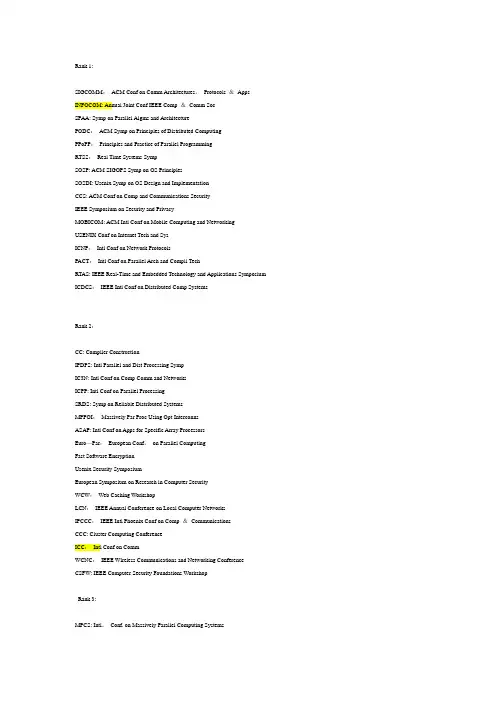
Rank 1:SIGCOMM：ACM Conf on Comm Architectures，Protocols ＆Apps INFOCOM: Annual Joint Conf IEEE Comp ＆Comm SocSPAA: Symp on Parallel Algms and ArchitecturePODC：ACM Symp on Principles of Distributed ComputingPPoPP：Principles and Practice of Parallel ProgrammingRTSS：Real Time Systems SympSOSP: ACM SIGOPS Symp on OS PrinciplesSOSDI: Usenix Symp on OS Design and ImplementationCCS: ACM Conf on Comp and Communications SecurityIEEE Symposium on Security and PrivacyMOBICOM: ACM Intl Conf on Mobile Computing and NetworkingUSENIX Conf on Internet Tech and SysICNP：Intl Conf on Network ProtocolsPACT：Intl Conf on Parallel Arch and Compil TechRTAS: IEEE Real-Time and Embedded Technology and Applications Symposium ICDCS：IEEE Intl Conf on Distributed Comp SystemsRank 2：CC: Compiler ConstructionIPDPS: Intl Parallel and Dist Processing SympIC3N: Intl Conf on Comp Comm and NetworksICPP: Intl Conf on Parallel ProcessingSRDS: Symp on Reliable Distributed SystemsMPPOI：Massively Par Proc Using Opt InterconnsASAP: Intl Conf on Apps for Specific Array ProcessorsEuro—Par：European Conf。

Manuals+— User Manuals Simplified.Mytrix GMS-15 RGB Gaming Mousepad Large Cherry Pink User GuideHome » mytrix » Mytrix GMS-15 RGB Gaming Mousepad Large Cherry Pink User GuideContents1 Mytrix GMS-15 RGB Gaming Mousepad Large CherryPink2 INTERFACE INSTRUCTIONS3 RGB SETTINGS4 TECHNICAL SPECIFICATION5 Documents / Resources6 Related PostsMytrix GMS-15 RGB Gaming Mousepad Large Cherry PinkThank you for buying Mytrix RGB mouse pad GMS-15. It supports a plug-andplay USB interface conveniently and there are a total of 14 light modes to meet your preference.INTERFACE INSTRUCTIONS1. RGB Light Mode Selecting Button2. Breathable Waterproof Micro-Texture Cloth Surface3. Non-slip Rubber Base4. RGB Light EdgeCONNECTIONPlug the detachable Type-C to USB-A cable into the mouse pad and turn on the SWITCH button.RGB SETTINGSFunctions:Select the Light Mode:1. RGB Light Mode Selecting Button2. Breathable Waterproof Micro-Texture Cloth Surface3. Non-slip Rubber Base4. RGB Light EdgePlug the detachable Type-C to USB-A cable into the mouse pad and turn on the SWITCH button. Press the SWITCH button to switch from 14 light modes in sequenceAdjust the Brightness:Double press the fingerprint icon to switch between the high and low brightness of the current light modeACCESSORY LISTThe product comes with a 1-year limited warranty. Our goal is to achieve total customer satisfaction, we will do our best to understand our customer’s requirements and always meet the requirements. If you have any questions, please do not hesitate to contact us via *****************. We will be more than happy to assist you.Company: Mytrix Technology LLCCustomer Service: +1-978-496-8821Email: *****************Web: Address: 13 Garabedian Dr. Unit C,Salem NH 03079Documents / ResourcesMytrix GMS-15 RGB Gaming Mousepad Large Cherry Pink [pdf] User GuideGMS-15 RGB Gaming Mousepad Large Cherry Pink, GMS-15, RGB Gaming Mousepad LargeCherry Pink, Gaming Mousepad Large Cherry Pink, Mousepad Large Cherry Pink, Large Cherry Pink, Cherry Pink, PinkManuals+,。

A Large-Scale Study of Flash Memory Failures in the FieldJustin Meza Carnegie Mellon University meza@Qiang WuFacebook,Inc.qwu@Sanjeev KumarFacebook,Inc.skumar@Onur MutluCarnegie Mellon Universityonur@ABSTRACTServers useflash memory based solid state drives(SSDs)as a high-performance alternative to hard disk drives to store per-sistent data.Unfortunately,recent increases inflash density have also brought about decreases in chip-level reliability.In a data center environment,flash-based SSD failures can lead to downtime and,in the worst case,data loss.As a result, it is important to understandflash memory reliability char-acteristics overflash lifetime in a realistic production data center environment running modern applications and system software.This paper presents thefirst large-scale study offlash-based SSD reliability in thefield.We analyze data collected across a majority offlash-based solid state drives at Facebook data centers over nearly four years and many millions of operational hours in order to understand failure properties and trends of flash-based SSDs.Our study considers a variety of SSD char-acteristics,including:the amount of data written to and read fromflash chips;how data is mapped within the SSD address space;the amount of data copied,erased,and discarded by the flash controller;andflash board temperature and bus power. Based on ourfield analysis of howflash memory errors man-ifest when running modern workloads on modern SSDs,this paper is thefirst to make several major observations:(1) SSD failure rates do not increase monotonically withflash chip wear;instead they go through several distinct periods corresponding to how failures emerge and are subsequently detected,(2)the effects of read disturbance errors are not prevalent in thefield,(3)sparse logical data layout across an SSD’s physical address space(e.g.,non-contiguous data),as measured by the amount of metadata required to track logical address translations stored in an SSD-internal DRAM buffer, can greatly affect SSD failure rate,(4)higher temperatures lead to higher failure rates,but techniques that throttle SSD operation appear to greatly reduce the negative reliability im-pact of higher temperatures,and(5)data written by the op-erating system toflash-based SSDs does not always accurately indicate the amount of wear induced onflash cells due to op-timizations in the SSD controller and buffering employed in the system software.We hope that thefindings of thisfirst large-scaleflash memory reliability study can inspire others to develop other publicly-available analyses and novelflash reliability solutions.Permission to make digital or hard copies of part or all of this work for personal or classroom use is granted without fee provided that copies are not made or distributed for profit or commercial advantage,and that copies bear this notice and the full ci-tation on thefirst page.Copyrights for third-party components of this work must be honored.For all other uses,contact the owner/author(s).Copyright is held by the author/owner(s).SIGMETRICS’15,June15–19,2015,Portland,OR,USA.ACM978-1-4503-3486-0/15/06./10.1145/2745844.2745848.Categories and Subject DescriptorsB.3.4.[Hardware]:Memory Structures—Reliability,Test-ing,and Fault-ToleranceKeywordsflash memory;reliability;warehouse-scale data centers1.INTRODUCTIONServers useflash memory for persistent storage due to the low access latency offlash chips compared to hard disk drives. Historically,flash capacity has lagged behind hard disk drive capacity,limiting the use offlash memory.In the past decade, however,advances in NANDflash memory technology have increasedflash capacity by more than1000×.This rapid in-crease inflash capacity has brought both an increase inflash memory use and a decrease inflash memory reliability.For example,the number of times that a cell can be reliably pro-grammed and erased before wearing out and failing dropped from10,000times for50nm cells to only2,000times for20nm cells[28].This trend is expected to continue for newer gen-erations offlash memory.Therefore,if we want to improve the operational lifetime and reliability offlash memory-based devices,we mustfirst fully understand their failure character-istics.In the past,a large body of prior work examined the failure characteristics offlash cells in controlled environments using small numbers e.g.,tens)of rawflash chips(e.g.,[36,23,21, 27,22,25,16,33,14,5,18,4,24,40,41,26,31,30,37,6,11, 10,7,13,9,8,12,20]).This work quantified a variety offlash cell failure modes and formed the basis of the community’s un-derstanding offlash cell reliability.Yet prior work was limited in its analysis because these studies:(1)were conducted on small numbers of rawflash chips accessed in adversarial man-ners over short amounts of time,(2)did not examine failures when using real applications running on modern servers and instead used synthetic access patterns,and(3)did not account for the storage software stack that real applications need to go through to accessflash memories.Such conditions assumed in these prior studies are substantially different from those expe-rienced byflash-based SSDs in large-scale installations in the field.In such large-scale systems:(1)real applications access flash-based SSDs in different ways over a time span of years, (2)applications access SSDs via the storage software stack, which employs various amounts of buffering and hence affects the access pattern seen by theflash chips,(3)flash-based SSDs employ aggressive techniques to reduce device wear and to cor-rect errors,(4)factors in platform design,including how many SSDs are present in a node,can affect the access patterns to SSDs,(5)there can be significant variation in reliability due to the existence of a very large number of SSDs andflash chips.All of these real-world conditions present in large-scalePlatform SSDs PCIePer SSDCapacity Age(years)Data written Data read UBERA1v1,×4720GB 2.4±1.027.2TB23.8TB5.2×10−10B248.5TB45.1TB2.6×10−9C1v2,×41.2TB 1.6±0.937.8TB43.4TB1.5×10−10D218.9TB30.6TB5.7×10−11E13.2TB0.5±0.523.9TB51.1TB5.1×10−11F214.8TB18.2TB1.8×10−10Table1:The platforms examined in our study.PCIe technology is denoted by vX,×Y where X=version and Y=number of lanes.Data was collected over the entire age of the SSDs.Data written and data read are to/from the physical storage over an SSD’s lifetime.UBER=uncorrectable bit error rate(Section3.2).rection and forwards the result to the host’s OS.Errors that are not correctable by the driver result in data loss.1Our SSDs allow us to collect information only on large er-rors that are uncorrectable by the SSD but correctable by the host.For this reason,our results are in terms of such SSD-uncorrectable but host-correctable errors,and when we refer to uncorrectable errors we mean these type of errors.We refer to the occurrence of such uncorrectable errors in an SSD as an SSD failure.2.3The SystemsWe examined the majority offlash-based SSDs in Face-book’s serverfleet,which have operational lifetimes extend-ing over nearly four years and comprising many millions of SSD-days of usage.Data was collected over the lifetime of the SSDs.We found it useful to separate the SSDs based on the type of platform an SSD was used in.We define a platform as a combination of the device capacity used in the system,the PCIe technology used,and the number of SSDs in the system. Table1characterizes the platforms we examine in our study. We examined a range of high-capacity multi-level cell(MLC)flash-based SSDs with capacities of720GB,1.2TB,and3.2TB. The technologies we examined spanned two generations of PCIe,versions1and2.Some of the systems in thefleet em-ployed one SSD while others employed two.Platforms A and B contain SSDs with around two or more years of operation and represent16.6%of the SSDs examined;Platforms C and D contain SSDs with around one to two years of operation and represent50.6%of the SSDs examined;and Platforms E and F contain SSDs with around half a year of operation and represent around22.8%of the SSDs examined.2.4Measurement MethodologyTheflash devices in ourfleet contain registers that keep track of statistics related to SSD operation(e.g.,number of bytes read,number of bytes written,number of uncorrectable errors).These registers are similar to,but distinct from,the standardized SMART data stored by some SSDs to monitor their reliability characteristics[3].The values in these regis-ters can be queried by the host machine.We use a collector script to retrieve the raw values from the SSD and parse them into a form that can be curated in a Hive[38]table.This process is done in real time every hour.The scale of the systems we analyzed and the amount of data being collected posed challenges for analysis.To process the many millions of SSD-days of information,we used a cluster of machines to perform a parallelized aggregation of the data stored in Hive using MapReduce jobs in order to get a set of 1We do not examine the rate of data loss in this work.lifetime statistics for each of the SSDs we analyzed.We then processed this summary data in R[2]to collect our results.2.5Analytical MethodologyOur infrastructure allows us to examine a snapshot of SSD data at a point in time(i.e.,our infrastructure does not store timeseries information for the many SSDs in thefleet).This limits our analysis to the behavior of thefleet of SSDs at a point in time(for our study,we focus on a snapshot of SSD data taken during November2014).Fortunately,the number of SSDs we examine and the diversity of their characteristics allow us to examine how reliability trends change with vari-ous characteristics.When we analyze an SSD characteristic (e.g.,the amount of data written to an SSD),we group SSDs into buckets based on their value for that characteristic in the snapshot and plot the failure rate for SSDs in each bucket. For example,if an SSD s is placed in a bucket for N TB of data written,it is not also placed in the bucket for(N−k)TB of data written(even though at some point in its life it did have only(N−k)TB of data written).When performing bucketing,we round the value of an SSD’s characteristic to the nearest bucket and we eliminate buckets that contain less than0.1%of the SSDs analyzed to have a statistically sig-nificant sample of SSDs for our measurements.In order to express the confidence of our observations across buckets that contain different numbers of servers,we show the95th per-centile confidence interval for all of our data(using a binomial distribution when considering failure rates).We measure SSD failure rate for each bucket in terms of the fraction of SSDs that have had an uncorrectable error compared to the total number of SSDs in that bucket.3.BASELINE STATISTICSWe willfirst focus on the overall error rate and error distri-bution among the SSDs in the platforms we analyze and then examine correlations between different failure events.3.1Bit Error RateThe bit error rate(BER)of an SSD is the rate at which er-rors occur relative to the amount of information that is trans-mitted from/to the SSD.BER can be used to gauge the relia-bility of data transmission across a medium.We measure the uncorrectable bit error rate(UBER)from the SSD as:UBER=Uncorrectable errorsBits accessedForflash-based SSDs,UBER is an important reliability met-ric that is related to the SSD lifetime.SSDs with high UBERs are expected to have more failed cells and encounter more(se-vere)errors that may potentially go undetected and corruptdata than SSDs with low UBERs.Recent work by Grupp et al.examined the BER of raw MLCflash chips(without per-forming error correction in theflash controller)in a controlled environment[20].They found the raw BER to vary from 1×10−1for the least reliableflash chips down to1×10−8 for the most reliable,with most chips having a BER in the 1×10−6to1×10−8range.Their study did not analyze the effects of the use of chips in SSDs under real workloads andsystem software.Table1shows the UBER of the platforms that we examine. Wefind that forflash-based SSDs used in servers,the UBER ranges from2.6×10−9to5.1×10−11.While we expect that the UBER of the SSDs that we measure(which correct small errors,perform wear leveling,and are not at the end of their rated life but still being used in a production environment) should be less than the raw chip BER in Grupp et al.’s study (which did not correct any errors in theflash controller,exer-cisedflash chips until the end of their rated life,and accessed flash chips in an adversarial manner),wefind that in some cases the BERs were within around one order of magnitude of each other.For example,the UBER of Platform B in our study,2.6×10−9,comes close to the lower end of the raw chip BER range reported in prior work,1×10−8.Thus,we observe that inflash-based SSDs that employ error correction for small errors and wear leveling,the UBER ranges from around1/10to1/1000×the raw BER of similarflash chips examined in prior work[20].This is likely due to the fact that ourflash-based SSDs correct small errors,perform wear leveling,and are not at the end of their rated life.As a result,the error rate we see is smaller than the error rate the previous study observed.As shown by the SSD UBER,the effects of uncorrectable errors are noticeable across the SSDs that we examine.We next turn to understanding how errors are distributed amonga population of SSDs and how failures occur within SSDs.3.2SSD Failure Rate and Error CountFigure2(top)shows the SSD incidence failure rate within each platform–the fraction of SSDs in each platform that have reported at least one uncorrectable error.Wefind that SSD failures are relatively common events with between4.2% and34.1%of the SSDs in the platforms we examine reporting uncorrectable errors.Interestingly,the failure rate is much lower for Platforms C and E despite their comparable amounts of data written and read(cf.Table1).This suggests that there are differences in the failure process among platforms.We analyze which factors play a role in determining the occurrence of uncorrectable errors in Sections4and5.Figure2(bottom)shows the average yearly uncorrectable error rate among SSDs within the different platforms–the sum of errors that occurred on all servers within a platform over12months ending in November2014divided by the num-ber of servers in the platform.The yearly rates of uncor-rectable errors on the SSDs we examined range from15,128 for Platform D to978,806for Platform B.The older Platforms A and B have a higher error rate than the younger Platforms C through F,suggesting that the incidence of uncorrectable errors increases as SSDs are utilized more.We will examine this relationship further in Section4.Platform B has a much higher average yearly rate of un-correctable errors(978,806)compared to the other platforms (the second highest amount,for Platform A,is106,678).We find that this is due to a small number of SSDs having amuchA B C D E FSSDfailurerate..2.4.6.81.A B C D E FYearlyuncorrectableerrorsperSSDe+4e+58e+5Figure2:The failure rate(top)and average yearly uncorrectable errors per SSD(bottom),among SSDs within each platform.higher number of errors in that platform:Figure3quantifies the distribution of errors among SSDs in each platform.The x axis is the normalized SSD number within the platform,with SSDs sorted based on the number of errors they have had over their lifetime.The y axis plots the number of errors for a given SSD in log scale.For every platform,we observe that the top 10%of SSDs with the most errors have over80%of all un-correctable errors seen for that platform.For Platforms B,C, E,and F,the distribution is even more skewed,with10%of SSDs with errors making up over95%of all observed uncor-rectable errors.We alsofind that the distribution of number of errors among SSDs in a platform is similar to that of a Weibull distribution with a shape parameter of0.3and scale parameter of5×103.The solid black line on Figure3plots this distribution.An explanation for the relatively large differences in errors per machine could be that error events are correlated.Exam-ining the data shows that this is indeed the case:during a recent two weeks,99.8%of the SSDs that had an error during thefirst week also had an error during the second week.We therefore conclude that an SSD that has had an error in the past is highly likely to continue to have errors in the future. With this in mind,we next turn to understanding the correla-tion between errors occurring on both devices in the two-SSD systems we examine.3.3Correlations Between Different SSDsGiven that some of the platforms we examine have twoflash-based SSDs,we are interested in understanding if the likeli-directly to flash cells),cells are read,programmed,and erased,and unreliable cells are identified by the SSD controller,re-sulting in an initially high failure rate among devices.Figure 4pictorially illustrates the lifecycle failure pattern we observe,which is quantified by Figure 5.Figure 5plots how the failure rate of SSDs varies with theamount of data written to the flash cells.We have groupedthe platforms based on the individual capacity of their SSDs.Notice that across most platforms,the failure rate is low whenlittle data is written to flash cells.It then increases at first(corresponding to the early detection period,region 1in thefigures),and decreases next (corresponding to the early failureperiod,region 2in the figures).Finally,the error rate gener-ally increases for the remainder of the SSD’s lifetime (corre-sponding to the useful life and wearout periods,region 3inthe figures).An obvious outlier for this trend is Platform C –in Section 5,we observe that some external characteristics ofthis platform lead to its atypical lifecycle failure pattern.Note that different platforms are in different stages in theirlifecycle depending on the amount of data written to flashcells.For example,SSDs in Platforms D and F,which havethe least amount of data written to flash cells on average,aremainly in the early detection or early failure periods.On theother hand,SSDs in older Platforms A and B,which havemore data written to flash cells,span all stages of the lifecyclefailure pattern (depicted in Figure 4).For SSDs in PlatformA,we observe up to an 81.7%difference between the failurerates of SSDs in the early detection period and SSDs in thewearout period of the lifecycle.As explained before and as depicted in Figure 4,the lifecy-cle failure rates we observe with the amount of data writtento flash cells does not follow the conventional bathtub curve.In particular,the new early detection period we observe acrossthe large number of devices leads us to investigate why this“early detection period”behavior exists.Recall that the earlydetection period refers to failure rate increasing early in life-time (i.e.,when a small amount of data is written to the SSD).After the early detection period,failure rate starts decreasing.We hypothesize that this non-monotonic error rate behav-ior during and after the early detection period can be ac-counted for by a two-pool model of flash blocks:one poolof blocks,called the weaker pool ,consists of cells whose errorrate increases much faster than the other pool of blocks,called the stronger pool .The weaker pool quickly generates uncor-rectable errors (leading to increasing failure rates observed in the early detection period as these blocks keep failing).The cells comprising this pool ultimately fail and are taken out of use early by the SSD controller.As the blocks in the weaker pool are exhausted,the overall error rate starts decreasing (as we observe after the end of what we call the early detection period )and it continues to decrease until the more durable blocks in the stronger pool start to wear out due to typical use.We notice a general increase in the duration of the lifecycle periods (in terms of data written)for SSDs with larger capac-ities.For example,while the early detection period ends after around 3TB of data written for 720GB and 1.2TB SSDs (in Platforms A,B,C,and D),it ends after around 10TB of data written for 3.2TB SSDs (in Platforms E and F).Similarly,the early failure period ends after around 15TB of data written for 720GB SSDs (in Platforms A and B),28TB for 1.2TB SSDs (in Platforms C and D),and 75TB for 3.2TB SSDs (in Platforms E and F).This is likely due to the more flexibility a higher-capacity SSD has in reducing wear across a larger number of flash cells.4.2Data Read from Flash Cells Similar to data written ,our framework allows us to measure the amount of data directly read from flash cells over each SSD’s lifetime.Prior works in controlled environments have shown that errors can be induced due to read-based access patterns [5,32,6,8].We are interested in understanding how prevalent this effect is across the SSDs we examine.Figure 6plots how failure rate of SSDs varies with the amount of data read from flash cells.For most platforms (i.e.,A,B,C,and F),the failure rate trends we see in Figure 6are similar to those we observed in Figure 5.We find this similar-ity when the average amount of data written to flash cells by SSDs in a platform is more than the average amount of data read from the flash cells.Platforms A,B,C,and F show this behavior.22Though Platform B has a set of SSDs with a large amount of data read,the average amount of data read across all SSDs in this platform is less than the average amount of data written.0e+004e+138e+13Data written (B)0.000.501.00S S D f a i l u r e r a t e ●Platform B0.0e+00 1.0e+14Data written (B)0.000.501.00S S D f a i l u r e r a te ●Platform D0.0e+00 1.5e+14 3.0e+14Data written (B)0.000.501.00S S D f a i l u r e r a t e ●Platform E Platform F Figure 5:SSD failure rate vs.the amount of data written to flash cells.SSDs go through several distinct phases throughout their life:increasing failure rates during early detection of less reliable cells (1),decreasing failure rates during early cell failure and subsequent removal (2),and eventually increasing error rates during cell wearout (3).0.0e+00 1.0e+14 2.0e+14Data read (B)0.000.501.00S S D f a i l u r e r a t e ●Platform B0.0e+00 1.0e+142.0e+14Data read (B)0.000.501.00S S D f a i l u r e r a te ●Platform C Platform D 0.0e+00 1.5e+14Data read (B)0.000.501.00S S D f a i l u r e r a t e ●Platform E Platform F Figure 6:SSD failure rate vs.the amount of data read from flash cells.SSDs in Platform E,where over twice as much data is read from flash cells as written to flash cells,do not show failures dependent on the amount of data read from flash cells.In Platform D,where more data is read from flash cells thanwritten to flash cells (30.6TB versus 18.9TB,on average),wenotice error trends associated with the early detection andearly failure periods.Unfortunately,even though devices inPlatform D may be prime candidates for observing the occur-rence of read disturbance errors (because more data is readfrom flash cells than written to flash cells),the effects of earlydetection and early failure appear to dominate the types oferrors observed on this platform.In Platform E,however,over twice as much data is readfrom flash cells as written to flash cells (51.1TB versus 23.9TBon average).In addition,unlike Platform D,devices in Plat-form E display a diverse amount of utilization.Under theseconditions,we do not observe a statistically significant differ-ence in the failure rate between SSDs that have read the mostamount of data versus those that have read the least amountof data.This suggests that the effect of read-induced errors inthe SSDs we examine is not predominant compared to othereffects such as write-induced errors.This corroborates priorflash cell analysis that showed that most errors occur due toretention effects and not read disturbance [32,11,12].4.3Block ErasesBefore new data can be written to a page in flash mem-ory,the entire block needs to be first erased.3Each erasewears out the block as shown in previous works [32,11,12].Our infrastructure tracks the average number of blocks erasedwhen an SSD controller performs garbage collection .Garbagecollection occurs in the background and erases blocks to en-sure that there is enough available space to write new data.The basic steps involved in garbage collection are:(1)select-ing blocks to erase (e.g.,blocks with many unused pages),(2)copying pages from the selected block to a free area,and (3)erasing the selected block [29].While we do not have statisticson how frequently garbage collection is performed,we exam-ine the number of erases per garbage collection period metricas an indicator of the average amount of erasing that occurswithin each SSD.We examined the relationship between the number of erasesperformed versus the failure rate (not plotted).Across the3Flash pages (around 8KB in size)compose each flash block.A flash block is around 128×8KB flash pages.SSDs we examine,we find that the failure trends in terms of erases are correlated with the trends in terms of data written (shown in Figure 5).This behavior reflects the typical opera-tion of garbage collection in SSD controllers:As more data is written,wear must be leveled across the flash cells within an SSD,requiring more blocks to be erased and more pages to be copied to different locations (an effect we analyze next).4.4Page Copies As data is written to flash-based SSDs,pages are copied to free areas during garbage collection in order to free up blocks with unused data to be erased and to more evenly level wear across the flash chips.Our infrastructure measures the num-ber of pages copied across an SSD’s lifetime.We examined the relationship between the number of pages copied versus SSD failure rate (not plotted).Since the page copying process is used to free up space to write data and also to balance the wear due to writes,its operation is largely dic-tated by the amount of data written to an SSD.Accordingly,we observe similar SSD failure rate trends with the number ofcopied pages (not plotted)as we observed with the amount ofdata written to flash cells (shown in Figure 5).4.5Discarded Blocks Blocks are discarded by the SSD controller when they are deemed unreliable for further use.Discarding blocks affects the usable lifetime of a flash-based SSD by reducing the amount of over-provisioned capacity of the SSD.At the same time,dis-carding blocks has the potential to reduce the amount of errors generated by an SSD,by preventing unreliable cells from being accessed.Understanding the reliability effects of discarding blocks is important,as this process is the main defense that SSD controllers have against failed cells and is also a major impediment for SSD lifetime.Figure 7plots the SSD failure rate versus number of dis-carded blocks over the SSD’s lifetime.For SSDs in most plat-forms,we observe an initially decreasing trend in SSD failure rate with respect to the number of blocks discarded followed by an increasing and then finally decreasing failure rate trend.We attribute the initially high SSD failure rate when few blocks have been discarded to the two-pool model of flash cell failure discussed in Section 4.1.In this case,the weaker pool of flash blocks (corresponding to weak blocks that fail。

文案大全
实用标准文档
序号 1 2 3 4 5 6 7 8 9 10 11 12 13 14 15 16 17
刊物名称(以期刊名称的拼音为序) 总被引频次
电子学报（英文版、中文版）
中文版 1676
高技术通讯（英文版、中文版） 计算机辅助设计与图形学学报 计算机工程 计算机集成制造系统 J COMPUT SCI & TECH 计算机学报 计算机研究与发展 计算数学（英） 科学通报（英文版、中文版） 模式识别与人工智能 软件学报 系统仿真学报 系统工程理论与实践
数学类第 4 名 综合类第 1 名
计算机类第 10 名 计算机类第 2 名 电子类第 7 名 信息类第 7 名 信息类第 3 名 计算机类第 16 名
综合类第 10 名
计算机类第 7 名 计算机类第 6 名
综合类第 11 名
计算机类第 9 名 计算机类第 18 名 计算机类第 20 名 计算机类第 21 名
28 IEEE/ACM Design Automation Conference
国际计算语言学会年会，是本领域最权威的国际学术会 议之一，每年举办一次 计算语言学会议，也是本领域最权威的国际学术会议之 一，两年一次 是语音和声学信号处理领域最权威的国际学术会议之 一，也是图像、视频信号处理领域的权威会议之一，每 年举办一次 自然语言处理亚洲联盟主办的国际会议，是自然语言处 理领域亚洲区域最有影响的学术会议，基本是每年举办 一次
网络测量领域顶级的专业会议
网络测量
下一代互联网研究 rank1
中心
12 ICCV: IEEE International Conference on
Computer Vision
领域顶级国际会议，录取率 20%左右，2 年一次，中国 计算机视觉，模式

最新无线网络领域顶级国际期刊、会议档次划分和介绍无线网络算是计算机(CS)和电子工程(EE)的一个交叉学科。

相关的会议和期刊通常没有物理生物等领域那些量化的影响因子排名。

但是有一点是公认的：会议影响力远大于期刊。

而会议之间也没有任何量化比较，只有人们默认的一些不成文的档次划分。

我读硕士和博士期间，组里对于会议和期刊档次的划分大致如下(其中加入了一些个人分析和评价)。

第一档：SIGCOMM, MobiComSIGCOMM是ACM老牌会议，其首席地位无可置疑。

SIGCOMM论文录用率在10%左右，收录的论文偏重系统和协议设计，极少有理论论文。

另外，每年收录的二三十篇论文中仅有1/5左右是无线网络，但这些论文的平均质量和影响力都很高。

MobiCom 专注于无线网络，每年收录30篇左右，录用率在10%~15%。

在2005年以前，MobiCom论文以理论加仿真占主导，所以一人一电脑就可搞定。

但之后随着WiFi硬件接口的公开和软件无线电平台的星期，做实验变得越来越容易，所以对于实验验证的要求越来越高，收录的论文也越来越偏系统设计测量之类。

2010年MobiCom的一位组委会成员感叹：MobiCom is becoming highly imbalanced. The systems guys clearly dominate the entire conference. Most of them don’t have the patience to read theory papers… If you don’t have any running code, it’s very hard to get in.第二档：MobiHoc, MobiSys, SIGMETRICSMobiHoc, MobiSys两个会议可以说是MobiCom下比肩而立的两兄弟。

MobiHoc偏理论，MobiSys偏系统和应用(特别是手机等移动计算系统)。

ACM的旗舰会议之一，也是网络领域顶级学术会议，内容侧重于有线网络，每年举办一次，录用率约为10%左右。
网络通信领域
下一代互联网研究中心
rank1
2
IEEE INFOCOM: The Conference on Computer Communications
IEEE计算机和通信分会联合年会，由IEEE计算机通信技术委员会和IEEE通信协会联合举办，是信息通信领域规模最大的顶尖国际学术会议，录用率约为16%左右。这个每年一度的会议的主要议题是计算机通信，重点是流量管理和协议。
16
软件学报
1598
0．919
计算机类第2名
17
通信学报
581
0．343
电子类第7名
18
系统仿真学报
867
0．415
信息类第7名
19
系统工程理论与实践
1372
0．533
信息类第3名
20
小型微型计算机系统
746
0．275
计算机类第16名
21
中国科学
E辑 403
E辑 0.444
综合类第10名
22
中国图象图形学报
ECCV: European Conference on Computer Vision
领域顶级国际会议，录取率25%左右，2年一次，中国大陆每年论文数不超过20篇
模式识别，计算机视觉，多媒体计算
数字媒体中心
rank1
15
DCC: Data Compression Conference
领域顶级国际会议，录取率很低，每年一次，目前完全国内论文极少
附4：计算所的限定供博士生选择的相关刊物
序号

中国计算机学会推荐国际学术会议和期刊目录（2015年）中国计算机学会中国计算机学会推荐国际学术期刊（计算机体系结构/并行与分布计算/存储系统）一、A类二、B类三、C类中国计算机学会推荐国际学术会议计算机体系结构/并行与分布计算/存储系统一、A类二、B类三、C类中国计算机学会推荐国际学术期刊（计算机网络）一、A类二、B类三、C类中国计算机学会推荐国际学术会议（计算机网络）一、A类二、B类三、C类中国计算机学会推荐国际学术期刊（网络与信息安全）一、A类二、B类三、C类中国计算机学会推荐国际学术会议（网络与信息安全）一、A类二、B类三、C类中国计算机学会推荐国际学术期刊（软件工程/系统软件/程序设计语言）一、A类二、B类三、C类中国计算机学会推荐国际学术会议（软件工程/系统软件/程序设计语言）一、A类二、B类三、C类中国计算机学会推荐国际学术期刊(数据库/数据挖掘/内容检索)一、A类二、B类三、C类中国计算机学会推荐国际学术会议(数据库／数据挖掘／内容检索)一、A类二、B类三、C类中国计算机学会推荐国际学术期刊（计算机科学理论）一、A类二、B类三、C类中国计算机学会推荐国际学术会议（计算机科学理论）一、A类二、B类三、C类中国计算机学会推荐国际学术期刊（计算机图形学与多媒体）一、A类二、B类三、C类中国计算机学会推荐国际学术会议（计算机图形学与多媒体）一、A类二、B类三、C类中国计算机学会推荐国际学术期刊（人工智能）一、A类。

ACM的具体介绍ACM(Association for Computing Machinery)国际计算机协会ACM 是一个国际科学教育计算机组织,它致力于发展在高级艺术、最新科学、工程技术和应用领域中的信息技术。

它强调在专业领域或在社会感兴趣的领域中培养、发展开放式的信息交换，推动高级的专业技术和通用标准的发展。

1947年，即世界第一台电子数字计算机(ENIAC)问世的第二年，ACM即成为第一个，也一直是世界上最大的科学教育计算机组织。

它的创立者和成员都是数学家和电子工程师，其中之一是约翰.迈克利(John.Mauchly)，他是ENIAC的发明家之一。

他们成立这个组织的初衷是为了计算机领域和新兴工业的科学家和技术人员能有一个共同交换信息、经验知识和创新思想的场合。

几十年的发展，ACM的成员们为今天我们所称之为“信息时代”作出了贡献。

他们所取得的成就大部分出版在ACM印刷刊物上并获得了ACM颁发的在各种领域中的杰出贡献奖。

例如：A.M.Turing奖和GranceMurr—ay Hopper奖。

ACM组织成员今天已达到九万人之多，他们大部分是专业人员、发明家、研究员、教育家、工程师和管理人员；三分之二以上的ACM成员，又是属于一个或多个SIGs(Special Interest Group)专业组织成员。

他们都对创造和应用信息技术有着极大的兴趣。

有些最大的最领先的计算机企业和信息工业也都是ACM 的成员。

ACM就像一个伞状的组织，为其所有的成员提供信息，包括最新的尖端科学的发展，从理论思想到应用的转换，提供交换信息的机会。

正象ACM建立时的初衷，它仍一直保持着它的发展“信息技术”的目标，ACM成为一个永久的更新最新信息领域的源泉。

编辑本段竞赛规则1比赛试题由6－10道试题组成，题目由英文或中文描述（中文题一半以上）。

2采用Windows环境，可使用的编程语言与编程工具为C/C++（VC++6.0）和pascal语言。

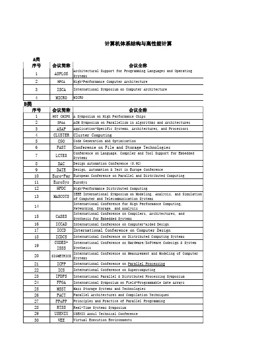
CCF推荐国际刊物会议列表2015中国计算机学会(CCF)推荐国际刊物会议列表20151.免费下载CSDN附件：2.存储在七⽜，不需CSDN：计算机体系结构/并⾏与分布计算/存储系统中国计算机学会推荐国际学术刊物　(计算机体系结构/并⾏与分布计算/存储系统）⼀、A类序号刊物简称刊物全称出版社⽹址1TOCS ACM Transactions on ComputerSystemsACM2TOC IEEE Transactions on Computers IEEE3TPDS IEEE Transactions on Parallel andDistributed SystemsIEEE4TCAD IEEE Transactions On Computer-AidedDesign Of Integrated Circuits AndSystemIEEE5TOS ACM Transactions on Storage ACM⼆、B类序号刊物简称刊物全称出版社⽹址1TACO ACM Transactions on Architecture andCode OptimizationACM2TAAS ACM Transactions on Autonomous and Adaptive SystemsACM3TODAES ACM Transactions on DesignAutomation of Electronic SystemsACM4TECS ACM Transactions on EmbeddedComputing SystemsACM5TRETS ACM Transactions on Reconfigurable Technology and SystemsACM6TVLSI IEEE Transactions on VLSI Systems IEEE7JPDC Journal of Parallel and DistributedComputingElsevier8PARCO Parallel Computing Elsevier9Performance Evaluation: An InternationalJournalElsevier10JSA Journal of Systems Architecture Elsevier三、C类序号刊物简称刊物全称出版社⽹址1Concurrency and Computation: Practiceand ExperienceWiley2DC Distributed Computing Springer 3FGCS Future Generation Computer Systems Elsevier 4Integration Integration, the VLSI Journal Elsevier5Microprocessors and Microsystems:Embedded Hardware DesignElsevier6JGC The Journal of Grid computing Springer 7TJSC The Journal of Supercomputing Springer8JETC The ACM Journal on EmergingTechnologies in Computing SystemsACM9JET Journal of Electronic Testing-Theory and ApplicationsSpringer10RTS Real-Time Systems Springer中国计算机学会推荐国际学术会议中国计算机学会推荐国际学术会议　(计算机体系结构/并⾏与分布计算/存储系统）⼀、A类序号会议简称会议全称出版社⽹址1ASPLOS Architectural Support for ProgrammingLanguages and Operating SystemsACM2FAST Conference on File and StorageTechnologiesUSENIX3HPCA High-Performance Computer Architecture IEEE4ISCA International Symposium on ComputerArchitectureACM /IEEE5MICRO MICRO IEEE/ACM6SC International Conference for HighPerformance Computing, Networking,Storage, and AnalysisIEEE7USENIXATCUSENIX Annul Technical Conference USENIX8PPoPP Principles and Practice of ParallelProgrammingACM⼆、B类序号会议简称会议全称出版社⽹址1HOT CHIPS ACM Symposium on HighPerformance ChipsIEEE2SPAA ACM Symposium on Parallelism in Algorithms and ArchitecturesACM3PODC ACM Symposium on Principles ofDistributed ComputingACM4CGO Code Generation and Optimization IEEE/ACM 5DAC Design Automation Conference ACM6DATE Design, Automation & Test in Europe ConferenceIEEE/ACM7EuroSys EuroSys ACM8HPDC High-Performance DistributedComputingIEEE9ICCD International Conference on ComputerDesignIEEE10ICCAD International Conference on Computer-Aided DesignIEEE/ACM11ICDCS International Conference on Distributed Computing SystemsIEEE12HiPEAC International Conference on High Performance and EmbeddedArchitectures and CompilersACM13SIGMETRICS International Conference onMeasurement and Modeling ofComputer SystemsACM14ICPP International Conference on Parallel ProcessingIEEE15ICS International Conference on SupercomputingACM16IPDPS International Parallel & Distributed Processing SymposiumIEEE17FPGA ACM/SIGDA International Symposiumon Field-Programmable Gate ArraysACM18 Performance International Symposium on Computer Performance, Modeling, Measurementsand EvaluationACM19LISA Large Installation systemAdministration ConferenceUSENIX20MSST Mass Storage Systems andTechnologiesIEEE21PACT Parallel Architectures and Compilation TechniquesIEEE/ACM23RTAS Real-Time and Embedded Technologyand Applications SymposiumIEEE24VEE Virtual Execution Environments ACM25CODES+ISSS ACM/IEEE Conf. Hardware/SoftwareCo-design and System SynthesisACM/ IEEE26ITC International Test Conference IEEE26ITC International Test Conference IEEE27SOCC ACM Symposium on Cloud Computing ACM三、C类序号会议简称会议全称出版社⽹址1CF ACM International Conference onComputing FrontiersACM2NOCS ACM/IEEE International Symposium onNetworks-on-ChipACM/IEEE3ASP-DAC Asia and South Pacific DesignAutomation ConferenceACM/IEEE4ASAP Application-Specific Systems, Architectures, and ProcessorsIEEE5CLUSTER Cluster Computing IEEE 6CCGRID Cluster Computing and the Grid IEEE7Euro-Par European Conference on Parallel and Distributed ComputingSpringer8ETS European Test Symposium IEEE9FPL Field Programmable Logic andApplicationsIEEE10FCCM Field-Programmable Custom Computing MachinesIEEE11GLSVLSI Great Lakes Symposium on VLSISystemsACM/IEEE12HPCC IEEE International Conference on High Performance Computing and CommunicationsIEEE13MASCOTS IEEE International Symposium onModeling, Analysis, and Simulation of Computer and TelecommunicationSystemsIEEE14NPC IFIP International Conference onNetwork and Parallel ComputingSpringer15ICA3PP International Conference on Algorithmsand Architectures for ParallelProcessingIEEE16CASES International Conference on Compilers, Architectures, and Synthesis forEmbedded SystemsACM17FPT International Conference on Field-Programmable TechnologyIEEE18HPC International Conference on HighPerformance ComputingIEEE/ ACM19ICPADS International Conference on Parallel and Distributed SystemsIEEE20ISCAS International Symposium on Circuits and SystemsIEEE21ISLPED International Symposium on Low Power Electronics and DesignACM/IEEE22ISPD International Symposium on PhysicalDesignACM23HotInterconnects Symposium on High-Performance InterconnectsIEEE24VTS VLSI Test Symposium IEEE25ISPA Sym. on Parallel and Distributed Processing with Applications26SYSTOR ACM SIGOPS International Systemsand Storage ConferenceACM27ATS IEEE Asian Test Symposium IEEE中国计算机学会推荐国际学术刊物　(计算机⽹络）⼀、A类序号刊物简称刊物全称出版社⽹址1TON IEEE/ACM Transactions on Networking IEEE, ACM2JSAC IEEE Journal of Selected Areas in CommunicationsIEEE3TMC IEEE Transactions on Mobile Computing IEEE⼆、B类序号刊物简称刊物全称出版社⽹址序号刊物简称刊物全称出版社⽹址1TOIT ACM Transactions on InternetTechnologyACM2TOMCCAP ACM Transactions on MultimediaComputing, Communications andApplicationsACM3TOSN ACM Transactions on Sensor Networks ACM 4CN Computer Networks Elsevier 5TOC IEEE Transactions on Communications IEEE6TWC IEEE Transactions on Wireless CommunicationsIEEE三、C类序号刊物简称刊物全称出版社⽹址1Ad hoc Networks Elsevier2CC Computer Communications Elsevier3TNSM IEEE Transactions on Network andService ManagementIEEE4IET Communications IET5JNCA Journal of Network and ComputerApplicationsElsevier6MONET Mobile Networks & Applications Springer 7Networks Wiley8PPNA Peer-to-Peer Networking andApplicationsSpringer9WCMC Wireless Communications & MobileComputingWiley.10Wireless Networks Springer中国计算机学会推荐国际学术会议　(计算机⽹络）⼀、A类序号会议简称会议全称出版社⽹址1MOBICOM ACM International Conference on Mobile Computing and NetworkingACM2SIGCOMM ACM International Conference on the applications, technologies, architectures,and protocols for computercommunicationACM3INFOCOM IEEE International Conference onComputer CommunicationsIEEE⼆、B类序号会议简称会议全称出版社⽹址1SenSys ACM Conference on EmbeddedNetworked Sensor SystemsACM2CoNEXT ACM International Conference onemerging Networking EXperiments and TechnologiesACM3SECON IEEE Communications SocietyConference on Sensor and Ad Hoc Communications and NetworksIEEE4IPSN International Conference on Information Processing in Sensor NetworksIEEE/ACM5ICNP International Conference on NetworkProtocolsIEEE6MobiHoc International Symposium on Mobile AdHoc Networking and ComputingACM/IEEE7MobiSys International Conference on MobileSystems, Applications, and ServicesACM8IWQoS International Workshop on Quality ofServiceIEEE9IMC Internet Measurement Conference ACM/USENIX10NOSSDAV Network and Operating System Supportfor Digital Audio and VideoACM11NSDI Symposium on Network System Designand ImplementationUSENIX三、C类序号会议简称会议全称出版社⽹址1ANCS Architectures for Networking and Communications SystemsACM/IEEE Formal Techniques for Networked and2FORTE Formal Techniques for Networked and Distributed SystemsSpringer3LCN IEEE Conference on Local ComputerNetworksIEEE4Globecom IEEE Global CommunicationsConference, incorporating the GlobalInternet SymposiumIEEE5ICC IEEE International Conference on CommunicationsIEEE6ICCCN IEEE International Conference onComputer Communications andNetworksIEEE7MASS IEEE International Conference on MobileAd hoc and Sensor SystemsIEEE8P2P IEEE International Conference on P2P ComputingIEEE9IPCCC IEEE International PerformanceComputing and CommunicationsConferenceIEEE10WoWMoM IEEE International Symposium on aWorld of Wireless Mobile and Multimedia NetworksIEEE11ISCC IEEE Symposium on Computers and CommunicationsIEEE12WCNC IEEE Wireless Communications &Networking ConferenceIEEE13Networking IFIP International Conferences onNetworkingIFIP14IM IFIP/IEEE International Symposium onIntegrated Network ManagementIFIP/IEEE15MSWiM International Conference on Modeling,Analysis and Simulation of Wireless andMobile SystemsACM16NOMS Asia-Pacific Network Operations and Management SymposiumIFIP/IEEE17HotNets The Workshop on Hot Topics inNetworksACM18WASA International Conference on Wireless Algorithms, Systems, and ApplicationsSpringer⽹络与信息安全中国计算机学会推荐国际学术刊物　(⽹络与信息安全）⼀、A类序号刊物简称刊物全称出版社⽹址1TDSC IEEE Transactions on Dependable andSecure ComputingIEEE2TIFS IEEE Transactions on InformationForensics and SecurityIEEE3Journal of Cryptology Springer⼆、B类序号刊物简称刊物全称出版社⽹址1TISSEC ACM Transactions on Information andSystem SecurityACM2Computers & Security Elsevier3Designs, Codes and Cryptography Springer4JCS Journal of Computer Security IOS Press三、C类序号刊物简称刊物全称出版社⽹址1CLSR Computer Law and Security Reports Elsevier2EURASIP Journal on InformationSecuritySpringer3IET Information Security IET4IMCS Information Management & ComputerSecurityEmerald4IMCSSecurityEmerald 5ISTR Information Security Technical Report Elsevier6IJISP International Journal of InformationSecurity and PrivacyIdea Group Inc7IJICS International Journal of Information andComputer SecurityInderscience8SCN Security and Communication Networks Wiley中国计算机学会推荐国际学术会议　(⽹络与信息安全）⼀、A类序号会议简称会议全称出版社⽹址1CCS ACM Conference on Computer and Communications SecurityACM2CRYPTO International Cryptology Conference Springer 3EUROCRYPTEuropean Cryptology Conference Springer4S&P IEEE Symposium on Security andPrivacyIEEE5USENIXSecurityUsenix Security SymposiumUSENIXAssociation⼆、B类序号会议简称会议全称出版社⽹址1ACSAC Annual Computer Security Applications ConferenceIEEE2ASIACRYPT Annual International Conference on theTheory and Application of Cryptologyand Information SecuritySpringer3ESORICS European Symposium on Research inComputer SecuritySpringer4FSE Fast Software Encryption Springer5NDSS ISOC Network and Distributed SystemSecurity SymposiumISOC6CSFW IEEE Computer Security Foundations WorkshopIEEE7RAID International Symposium on RecentAdvances in Intrusion DetectionSpringer8PKC International Workshop on Practice andTheory in Public Key CryptographySpringer9DSN The International Conference onDependable Systems and NetworksIEEE/IFIP10TCC Theory of Cryptography Conference Springer11SRDS IEEE International Symposium onReliableDistributed SystemsIEEE12CHES Workshop on Cryptographic HardwareandEmbedded SystemsSpringer三、C类序号会议简称会议全称出版社⽹址1WiSec ACM Conference on Security andPrivacy inWireless and Mobile NetworksACM2ACMMM&SECACM Multimedia and SecurityWorkshopACM3SACMAT ACM Symposium on Access ControlModels and TechnologiesACM4ASIACCS ACM Symposium on Information,Computer andCommunications SecurityACM5DRM ACM Workshop on Digital Rights ManagementACM6ACNS Applied Cryptography and NetworkSecuritySpringer7ACISP Australasia Conference on InformationSecurity and PrivacySpringer8DFRWS Digital Forensic Research Workshop Elsevier9FC Financial Cryptography and DataSecuritySpringer10DIMVA Detection of Intrusions and Malware & Vulnerability AssessmentSIDAR、GI、SpringerVulnerability Assessment Springer 11SECIFIP International InformationSecurity ConferenceSpringer 12IFIP WG 11.9IFIP WG 11.9 InternationalConferenceon Digital ForensicsSpringer 13ISC Information Security ConferenceSpringer 14ICICS International Conference onInformationand Communications SecuritySpringer15SecureComm International Conference on SecurityandPrivacy in Communication NetworksACM 16NSPW New Security Paradigms WorkshopACM 17CT-RSARSA Conference, Cryptographers'TrackSpringer 18SOUPSSymposium On Usable Privacy andSecurityACM 19HotSecUSENIX Workshop on Hot Topics inSecurityUSENIX 20SAC Selected Areas in CryptographySpringer 21TrustComIEEE International Conference on Trust,Security and Privacy in Computing and CommunicationsIEEE22PAMPassive and Active MeasurementConferenceSpringer 23PETSPrivacy Enhancing TechnologiesSymposiumSpringer 24International Conference on DigitalForensics & Cyber CrimeSpringer软件⼯程/系统软件/程序设计语⾔中国计算机学会推荐国际学术期刊 （软件⼯程/系统软件/程序设计语⾔）⼀、A 类序号刊物简称刊物全称出版社⽹址1TOPLASACM Transactions on ProgrammingLanguages & SystemsACM 2TOSEM ACM Transactions on Software Engineering Methodology ACM3TSE IEEE Transactions on Software EngineeringIEEE⼆、B 类序号刊物简称刊物全称出版社⽹址1ASE Automated Software Engineering Springer 2ESE Empirical Software Engineering Springer 3TSC IEEE Transactions on Service Computing IEEE 4IETS IET Software IET 5IST Information and Software Technology Elsevier6JFP Journal of Functional Programming Cambridge University Press7 Journal of Software: Evolution and Process Wiley 8JSS Journal of Systems and Software Elsevier 9RE Requirements Engineering Springer 10SCP Science of Computer Programming Elsevier 11SoSyM Software and System Modeling Springer 12SPE Software: Practice and Experience Wiley 13STVR Software Testing, Verification and ReliabilityWiley三、C 类序号刊物简称刊物全称出版社⽹址1CL Computer Languages, Systems and StructuresElsevier 2IJSEKE International Journal on Software Engineering and Knowledge Engineering World Scientific 3STTT International Journal on Software Tools for Technology TransferSpringer3STTT International Journal on Software Tools for Technology Transfer Springer 4JLAP Journal of Logic and Algebraic Programming Elsevier 5JWE Journal of Web Engineering Rinton Press 6SOCA Service Oriented Computing and Applications Springer 7SQJ Software Quality Journal Springer8TPLP Theory and Practice of Logic Programming Cambridge University Press中国计算机学会推荐国际学术会议（软件⼯程/系统软件/程序设计语⾔）⼀、A类序号会议简称会议全称出版社⽹址1FSE/ESEC ACM SIGSOFT Symposium on the Foundationof Software Engineering/ European SoftwareEngineering ConferenceACM2OOPSLA Conference on Object-OrientedProgramming Systems, Languages,and ApplicationsACM3ICSE International Conference onSoftware EngineeringACM/IEEE4OSDI USENIX Symposium onOperating Systems Designand ImplementationsUSENIX5PLDI ACM SIGPLAN Symposium on ProgrammingLanguage Design & ImplementationACM6POPL ACM SIGPLAN-SIGACTSymposium on Principlesof Programming LanguagesACM7SOSP ACM Symposium onOperating Systems PrinciplesACM8ASE International Conference onAutomated Software EngineeringIEEE/ACM⼆、B类序号会议简称会议全称出版社⽹址1ECOOP European Conference on Object-Oriented Programming2ETAPS European Joint Conferences on Theoryand Practice of SoftwareSpringer3FM World Congress on Formal Methods FME4ICPC IEEE International Conference onProgram ComprehensionIEEE5RE IEEE International RequirementEngineering ConferenceIEEE6CAiSE International Conference on AdvancedInformation Systems EngineeringSpringer7ICFP International Conference onFunction ProgrammingACM8LCTES International Conference on Languages,Compilers, Tools and Theory forEmbedded SystemsACM9MoDELS International Conference on Model DrivenEngineering Languages and SystemsACM, IEEE10CP International Conference on Principlesand Practice of Constraint ProgrammingSpringer11ICSOC International Conference on ServiceOriented ComputingSpringer12ICSME International Conference on SoftwareMaintenance and EvolutionIEEE13VMCAI International Conference on Verification,Model Checking, and Abstract InterpretationSpringer14ICWS International Conference on Web Services（Research Track）IEEE15SAS International Static Analysis Symposium Springer16ISSRE International Symposium on SoftwareReliability EngineeringIEEE17ISSTA International Symposium onSoftware Testing and AnalysisACM18Middleware Conference on middlewareACM/IFIP/18Middleware Conference on middleware ACM/IFIP/ USENIX19SANER International Conference on SoftwareAnalysis, Evolution, and ReengineeringIEEE20HotOS USENIX Workshop on Hot Topics inOperating SystemsUSENIX21ESEM International Symposium on EmpiricalSoftware Engineering and MeasurementACM/IEEE三、C类序号会议简称会议全称出版社⽹址1PASTE ACMSIGPLAN-SIGSOFT Workshopon Program Analysis for SoftwareTools and EngineeringACM2APLAS Asian Symposium on ProgrammingLanguages and SystemsSpringer3APSEC Asia-Pacific Software Engineering ConferenceIEEE4COMPSAC International Computer Software andApplications ConferenceIEEE5ICECCS IEEE International Conference onEngineering of Complex Computer SystemsIEEE6SCAM IEEE International Working Conferenceon Source Code Analysis and ManipulationIEEE7ICFEM International Conference on FormalEngineering MethodsSpringer8TOOLS International Conference on Objects,Models, Components, PatternsSpringer9PEPM ACM SIGPLAN Symposium on PartialEvaluation and Semantics BasedProgramming ManipulationACM10QRS The IEEE International Conference on Software Quality, Reliability and Security IEEE11SEKE International Conference on SoftwareEngineering and Knowledge EngineeringKSI12ICSR International Conference on Software Reuse Springer 13ICWE International Conference on Web Engineering Springer14SPIN International SPIN Workshop on ModelChecking of SoftwareSpringer15LOPSTR International Symposium on Logic-based Program Synthesis and Transformation Springer16TASE International Symposium on TheoreticalAspects of Software EngineeringIEEE17ICST The IEEE International Conference onSoftware Testing, Verification and ValidationIEEE18ATVA International Symposium on Automated Technology for Verification and Analysis Springer19ISPASS IEEE International Symposium onPerformance Analysis of Systems andSoftwareIEEE20SCC International Conference on ServiceComputingIEEE21ICSSP International Conference on Softwareand System ProcessISPA22MSR Working Conference on Mining Software Repositories IEEE/ACM 23REFSQ Requirements Engineering: Foundation for Software Quality Springer24WICSA Working IEEE/IFIP Conference onSoftware ArchitectureIEEE25EASE Evaluation and Assessment in SoftwareEngineeringACM数据库/数据挖掘/内容检索中国计算机学会推荐国际学术期刊（数据库/数据挖掘/内容检索）⼀、A类序号刊物简称刊物全称出版社⽹址1TODS ACM Transactions on Database Systems ACM2TOIS ACM Transactions on InformationSystemsACM2TOISSystemsACM3TKDE IEEE Transactions on Knowledge andData EngineeringIEEE4VLDBJ VLDB Journal Springer⼆、B类序号刊物简称刊物全称出版社⽹址1TKDD ACM Transactions onKnowledge Discovery from DataACM2AEI Advanced Engineering Informatics Elsevier 3DKE Data and Knowledge Engineering Elsevier4DMKD Data Mining andKnowledge DiscoverySpringer5EJIS European Journal of Information Systems6GeoInformatica Springer 7IPM Information Processing and Management Elsevier 8Information Sciences Elsevier 9IS Information Systems Elsevier10JASIST Journal of the American Society forInformation Science and TechnologyAmericanSociety forInformationScience andTechnology11JWS Journal of Web Semantics Elsevier12KIS Knowledge and Information Systems Springer13TWEB ACM Transactions on the Web ACM三、C类序号刊物简称刊物全称出版社⽹址1DPD Distributed and Parallel Databases Springer2I&M Information and Management Elsevier3IPL Information Processing Letters Elsevier4IR Information Retrieval Springer5IJCIS International Journal of CooperativeInformation SystemsWorldScientific6IJGIS International Journal of Geographical Information Science7IJIS International Journal of Intelligent Systems Wiley8IJKM International Journal of KnowledgeManagementIGI9IJSWIS International Journal on Semantic Web and Information SystemsIGI10JCIS Journal of Computer Information Systems IACIS 11JDM Journal of Database Management IGI-Global12JGITM Journal of Global Information Technology Management13JIIS Journal of Intelligent Information Systems Springer14JSIS Journal of Strategic Information Systems Elsevier中国计算机学会推荐国际学术会议（数据库/数据挖掘/内容检索）⼀、A类序号会议简称会议全称出版社⽹址1SIGMOD ACM Conference on Management ofDataACM2SIGKDD ACM Knowledge Discovery and DataMiningACM3SIGIR International Conference on ResearchonDevelopment in Information RetrievalACM4VLDB International Conference onVery Large Data BasesMorganKaufmann/ACM5ICDE IEEE International Conference onData EngineeringIEEE⼆、B类序号会议简称会议全称出版社⽹址1CIKM ACM International Conferenceon Information and KnowledgeManagementACM2PODS ACM SIGMOD Conference onPrinciples ACM2PODS Principlesof DB SystemsACM3DASFAA Database Systems for AdvancedApplicationsSpringer4ECML-PKDDEuropean Conference on MachineLearning and Principles andPractice of Knowledge Discoveryin DatabasesSpringer5ISWC IEEE International Semantic WebConferenceIEEE6ICDM International Conference on Data Mining IEEE7ICDT International Conference on DatabaseTheorySpringer8EDBT International Conference onExtending DB TechnologySpringer9CIDR International Conference onInnovation Database ResearchOnlineProceeding10SDM SIAM International Conference on DataMiningSIAM11WSDM ACM International Conference onWeb Search and Data MiningACM三、C类序号会议简称会议全称出版社⽹址1DEXA Database and Expert System Applications Springer2ECIR European Conference on IR Research Springer3WebDB International ACM Workshop onWeb and DatabasesACM4ER International Conference on ConceptualModelingSpringer5MDM International Conference on Mobile Data ManagementIEEE6SSDBM International Conference on Scientificand Statistical DB ManagementIEEE7WAIM International Conference on Web AgeInformation ManagementSpringer8SSTD International Symposium on Spatialand Temporal DatabasesSpringer9PAKDD Pacific-Asia Conference on KnowledgeDiscovery and Data MiningSpringer10APWeb The Asia Pacific Web Conference Springer11WISE Web Information Systems Engineering Springer12ESWC Extended Semantic Web Conference Elsevier计算机科学理论中国计算机学会推荐国际学术期刊（计算机科学理论）⼀、A类序号刊物简称刊物全称出版社⽹址1IANDC Information and Computation Elsevier2SICOMP SIAM Journal on Computing SIAM3TIT IEEE Transactions on Information Theory IEEE⼆、B类序号刊物简称刊物全称出版社⽹址1TALG ACM Transactions on Algorithms ACM2TOCL ACM Transactions on ComputationalLogicACM3TOMS ACM Transactions on MathematicalSoftwareACM4AlgorithmicaAlgorithmica Springer 5CC Computational complexity Springer 6FAC Formal Aspects of Computing Springer 7FMSD Formal Methods in System Design Springer 8INFORMS INFORMS Journal on Computing INFORMS9JCSS Journal of Computer and SystemElsevier9JCSS Journal of Computer and SystemSciencesElsevier10JGO Journal of Global Optimization Springer 11JSC Journal of Symbolic Computation Elsevier12MSCS Mathematical Structures in ComputerScienceCambridgeUniversityPress13TCS Theoretical Computer Science Elsevier三、C类序号刊物简称刊物全称出版社⽹址1APAL Annals of Pure and Applied Logic Elsevier2ACTA Acta Informatica Springer3DAM Discrete Applied Mathematics Elsevier4FUIN Fundamenta Informaticae IOS Press5LISP Higher-Order and SymbolicComputationSpringer6IPL Information Processing Letters Elsevier 7JCOMPLEXITYJournal of Complexity Elsevier8LOGCOM Journal of Logic and ComputationOxford University Press9Journal of Symbolic Logic Association for SymbolicLogic10LMCS Logical Methods in Computer Science LMCS11SIDMA SIAM Journal on Discrete Mathematics SIAM12Theory of Computing Systems Springer中国计算机学会推荐国际学术会议（计算机科学理论）⼀、A类序号会议简称会议全称出版社⽹址1STOC ACM Symposium on Theory ofComputingACM2FOCS IEEE Symposium on Foundations ofComputer ScienceIEEE3LICS IEEE Symposium on Logic inComputer ScienceIEEE4CAV Computer Aided Verification Springer⼆、B类序号会议简称会议全称出版社⽹址1SoCG ACM Symposium on ComputationalGeometryACM2SODA ACM-SIAM Symposium on DiscreteAlgorithmsSIAM3CADE/IJCAR Conference on AutomatedDeduction/The International JointConference on Automated ReasoningSpringer4CCC IEEE Conference on Computational ComplexityIEEE5ICALP International Colloquium onAutomata, Languages andProgrammingSpringer6CONCUR International Conference onConcurrency TheorySpringer7HSCC International Conference onHybrid Systems: Computation andControlSpringerand ACM8ESA European Symposium on Algorithms Springer三、C类序号会议简称会议全称出版社⽹址1CSL Computer Science Logic Springer2FSTTCS Foundations of Software Technologyand Theoretical ComputerScienceIndian AssociationforResearch inComputingScience3IPCO International Conference onInteger Programming andCombinatorial OptimizationSpringerCombinatorial Optimization4RTA International Conference onRewriting Techniques andApplicationsSpringer5ISAAC International Symposium onAlgorithmsand ComputationSpringer6MFCS Mathematical Foundations ofComputer ScienceSpringer7STACS Symposium on Theoretical Aspectsof Computer ScienceSpringer8FMCAD Formal Method in Computer-AidedDesignACM9SAT Theory and Applications ofSatisfiability TestingSpringer10ICTAC International Colloquium onTheoreticalAspects of ComputingSpringer计算机图形学与多媒体中国计算机学会推荐国际学术刊物（计算机图形学与多媒体）⼀、A类序号刊物简称刊物全称出版社⽹址1TOG ACM Transactions on Graphics ACM2TIP IEEE Transactions on Image Processing IEEE3TVCG IEEE Transactions on Visualization and Computer GraphicsIEEE⼆、B类序号刊物简称刊物全称出版社⽹址1TOMCCAP ACM Transactions on MultimediaComputing,Communications andApplicationACM2CAD Computer-Aided Design Elsevier 3CAGD Computer Aided Geometric Design Elsevier 4CGF Computer Graphics Forum Wiley 5GM Graphical Models Elsevier6TCSVT IEEE Transactions on Circuits andSystems forVideo TechnologyIEEE7TMM IEEE Transactions on Multimedia IEEE8JASA Journal of The Acoustical Society ofAmericaAIP9SIIMS SIAM Journal on Imaging Sciences SIAM10SpeechComSpeech Communication Elsevier三、C类序号刊物简称刊物全称出版社⽹址1CAVW Computer Animation and Virtual Worlds Wiley2C&G Computers & Graphics-UK Elsevier3CGTA Computational Geometry: Theory and ApplicationsElsevier4DCG Discrete & Computational Geometry Springer 5IET-IPR IET Image Processing IET 6IEEE Signal Processing Letter IEEE7JVCIR Journal of Visual Communication andImage RepresentationElsevier8MS Multimedia Systems Springer 9MTA Multimedia Tools and Applications Springer10SignalProcessingElsevier11SPIC Signal processing : imagecommunicationElsevier12TVC The Visual Computer Springer中国计算机学会推荐国际学术会议（计算机图形学与多媒体）。

学术会议排名一、A类序号会议名称论文集的出版社1. Special Interest Group on Data Communication(SIGCOMM) ACM录取率：9~13%2. Special Interest Group on Mobility of Sys-tems, Users, Data and Computing (MOBICOM) ACM录取率：~10%3. International Symposium on Mobile Ad Hoc Networking and Computing (MOBIHOC) ACM/IEEE录取率：<13%4. Special Interest Group on Measurement and Evaluation (SIGMETRICS) ACM录取率：<13%二、B类序号会议名称论文集的出版社1. International Conference on Network Protocols (ICNP) IEEE录取率：14~18%2. Conference on Computer Communications (INFOCOM) IEEE录取率：18~20%3. International World Wide Web (WWW)录取率：~15%4. International Conference on Embedded Networked SensorSystems (SenSys) ACM录取率：~15%5. USENIX Annual Technical Conference USENIX '09 January 9, 2009 full papers: <14 pages, short papers: <6 pages 录取率：12~16%6. Network and Distributed System Security Symposium (NDSS ) USENIX录取率：12~20%7. International Conference on Distributed Computing Systems (ICDCS) IEEE录取率：13~17%8. International Conference on Pervasive Computing and Communications (PerCom) IEEE '10 Paper submission: September 28, 2009录取率：9~17%三、C类序号会议名称论文集的出版社1. International Workshop on Quality of Service (IWQoS) IEEE录取率：~20%2. IEEE/ACM International Workshop on Grid Computing(Grid) IEEE/ACM录取率：~20%3. Symposium on Network System Design and Implementation (NDSI) USENIX录取率：~22%4. International Conferences on Networking (Networking) IFIP录取率：19~24%5. Conference on High Performance Computing, Networking and Storage (Supercomputing) IEEE/ACM录取率：22~29%6. International Conference on Information Processing in Sensor Networks (IPSN) ACM/IEEE录取率：15~18%四、其他会议序号会议名称论文集的出版社1. IFIP/IEEE International Symposium on Integrated Network Management(IM) IFIP/IEEE录取率：23~50%2. International Parallel & Distributed Processing Symposium (IPDPS) IEEE录取率：23~38%3. International Symposium on Modeling, Analysis and Simulation of Wireless and Mobile Systems (MSWiM) ACM 录取率：23~38%4. IEEE Communications Society Conference on Sensor and Ad Hoc Communications and Networks(SECON) IEEE 录取率：18~27%5. Network Operations and Management Symposium(MONS) IFIP/IEEE录取率：~26%6. Conference on Local Computer Networks (LCN) IEEE录取率：26~40%7. Formal Techniques for Networked and Distributed Systems FORTE录取率：30~70%8. IEEE Global Communications Conference, incorporating the Global Internet Symposium (Globecom) IEEE录取率：~35%9. International Conference on Communications (ICC) IEEE录取率：~35%10. SYMPOSIUM ON COMPUTERS AND COMMUNICATIONS (ISCC) IEEE录取率：~40%11. IEEE Semiannual Vehicular Technology Conference (VTC) IEEE。

计算机学科国际会议分级说明：本列表合并了UCLA、NUS、NTU、CCF、清华大学计算机系、上海交大计算机系认可的国际会议，分级时采用了“就高”的原则。

Rank #1(1) AAAI: AAAI Conference on Artificial IntelligenceRefs: UCLA(1) CCF(1) NTU(1) SJTU(1) TSINGHUA(1) NUS(1)(2) CCS: ACM Conf on Comp and Communications SecurityRefs: UCLA(1) CCF(1) NTU(1) SJTU(1) TSINGHUA(1) NUS(1)(3) CRYPTO: International Cryptology ConferenceRefs: UCLA(1) CCF(1) NTU(1) SJTU(1) TSINGHUA(1) NUS(1)(4) CVPR: IEEE Conf on Comp Vision and Pattern RecognitionRefs: UCLA(1) CCF(1) NTU(1) SJTU(1) TSINGHUA(1) NUS(1)(5) FOCS: IEEE Symp on Foundations of Computer ScienceRefs: UCLA(1) CCF(1) NTU(1) SJTU(1) TSINGHUA(1) NUS(1)(6) HPCA: IEEE Symp on High-Perf Comp ArchitectureRefs: UCLA(1) CCF(1) NTU(1) SJTU(1) TSINGHUA(1) NUS(1)(7) ICCV: International Conf on Computer VisionRefs: UCLA(1) CCF(1) NTU(1) SJTU(1) TSINGHUA(1) NUS(1)(8) ICDE: Intl Conf on Data EngineeringRefs: UCLA(1) CCF(1) NTU(1) SJTU(1) TSINGHUA(1) NUS(1)(9) ICML: Intl Conf on Machine LearningRefs: UCLA(1) CCF(1) NTU(1) SJTU(1) TSINGHUA(1) NUS(1)(10) ICSE: Intl Conf on Software EngineeringRefs: UCLA(1) CCF(1) NTU(1) SJTU(1) TSINGHUA(1) NUS(1)(11) IJCAI: International Joint Conference on Artificial IntelligenceRefs: UCLA(1) CCF(1) NTU(1) SJTU(1) TSINGHUA(1) NUS(1)(12) INFOCOM: Annual Joint Conf IEEE Comp & Comm SocRefs: UCLA(1) CCF(1) NTU(1) SJTU(1) TSINGHUA(1) NUS(1)(13) ISCA: ACM/IEEE Symp on Computer ArchitectureRefs: UCLA(1) CCF(1) NTU(1) SJTU(1) TSINGHUA(1) NUS(1)(14) MICRO: Intl Symp on MicroarchitectureRefs: UCLA(1) CCF(1) NTU(1) SJTU(1) TSINGHUA(1) NUS(1)(15) MOBICOM: ACM Intl Conf on Mobile Computing and NetworkingRefs: UCLA(1) CCF(1) NTU(1) SJTU(1) TSINGHUA(1) NUS(1)(16) OOPSLA: OO Programming Systems, Languages and ApplicationsRefs: UCLA(1) CCF(1) NTU(1) SJTU(1) TSINGHUA(1) NUS(1)(17) POPL: ACM-SIGACT Symp on Principles of Prog LangsRefs: UCLA(1) CCF(1) NTU(1) SJTU(1) TSINGHUA(1) NUS(1)(18) SIGCOMM: ACM Conf on Comm Architectures, Protocols & AppsRefs: UCLA(1) CCF(1) NTU(1) SJTU(1) TSINGHUA(1) NUS(1)(19) SIGGRAPH: ACM SIGGRAPH ConferenceRefs: UCLA(1) CCF(1) NTU(1) SJTU(1) TSINGHUA(1) NUS(1)(20) SIGMOD: ACM SIGMOD Conf on Management of DataRefs: UCLA(1) CCF(1) NTU(1) SJTU(1) TSINGHUA(1) NUS(1)(21) STOC: ACM Symp on Theory of ComputingRefs: UCLA(1) CCF(1) NTU(1) SJTU(1) TSINGHUA(1) NUS(1)(22) VLDB: Very Large Data BasesRefs: UCLA(1) CCF(1) NTU(1) SJTU(1) TSINGHUA(1) NUS(1)(23) ACL: Annual Meeting of the Association for Computational LinguisticsRefs: UCLA(1) CCF(2) NTU(1) SJTU(1) TSINGHUA(1) NUS(1)(24) ACM-MM: ACM Multimedia ConferenceRefs: UCLA(1) CCF(1) NTU(1) SJTU(1) TSINGHUA(2) NUS(1)(25) NIPS: Annual Conference on Neural Information Processing SystemsRefs: UCLA(1) CCF(2) NTU(1) SJTU(1) TSINGHUA(1) NUS(1)(26) PLDI: ACM SIGPLAN Symposium on Programming Language Design & Implementation Refs: UCLA(1) CCF(2) NTU(1) SJTU(1) TSINGHUA(1) NUS(1)(27) S&P: IEEE Symposium on Security and PrivacyRefs: UCLA(1) CCF(1) NTU(1) SJTU(1) TSINGHUA(2) NUS(1)(28) SIGMETRICS: ACM Conf on Meas. & Modelling of Comp SysRefs: UCLA(1) CCF(2) NTU(1) SJTU(1) TSINGHUA(1) NUS(1)(29) WWW: International World Wide Web ConferenceRefs: UCLA(1) CCF(2) NTU(1) SJTU(1) TSINGHUA(1) NUS(1)(30) FSE: ACM Conf on the Foundations of Software EngineeringRefs: UCLA(1) CCF(1) NTU(1) TSINGHUA(1) NUS(1)(31) ICDCS: International Conference on Distributed Computing SystemsRefs: UCLA(2) CCF(2) NTU(1) SJTU(1) TSINGHUA(2) NUS(1)(32) LICS: IEEE Symp on Logic in Computer ScienceRefs: UCLA(1) CCF(2) NTU(1) SJTU(1) TSINGHUA(2) NUS(1)(33) ASPLOS: Architectural Support for Programming Languages and Operating Systems Refs: UCLA(1) CCF(2) NTU(1) TSINGHUA(1) NUS(1)(34) COLT: Annual Conference on Computational Learning TheoryRefs: UCLA(1) CCF(2) NTU(1) TSINGHUA(1) NUS(1)(35) PODS: ACM SIGMOD Conf on Principles of DB SystemsRefs: UCLA(1) CCF(2) NTU(1) TSINGHUA(1) NUS(1)(36) PPoPP: Principles and Practice of Parallel ProgrammingRefs: UCLA(1) CCF(2) NTU(1) TSINGHUA(1) NUS(1)(37) SIGIR: ACM SIGIR Conf on Information RetrievalRefs: UCLA(1) CCF(2) NTU(1) SJTU(1) TSINGHUA(1)(38) SODA: ACM/SIAM Symp on Discrete AlgorithmsRefs: UCLA(1) CCF(2) NTU(1) TSINGHUA(1) NUS(1)(39) UAI: Conference on Uncertainty in AIRefs: UCLA(1) CCF(2) NTU(1) TSINGHUA(1) NUS(1)(40) DAC: Design Automation ConfRefs: UCLA(1) NTU(1) TSINGHUA(1) NUS(1)(41) KDD: Knowledge Discovery and Data MiningRefs: UCLA(1) NTU(1) TSINGHUA(1) NUS(1)(42) SOSP: ACM SIGOPS Symp on OS PrinciplesRefs: UCLA(1) NTU(1) TSINGHUA(1) NUS(1)(43) ICALP: International Colloquium on Automata, Languages and ProgrammingRefs: UCLA(2) CCF(2) NTU(2) SJTU(1) TSINGHUA(2) NUS(2)(44) IPDPS: Intl Parallel and Dist Processing SympRefs: UCLA(2) CCF(2) NTU(2) SJTU(1) TSINGHUA(3) NUS(2)(45) AAMAS: Intl Conf on Autonomous Agents and Multi-Agent SystemsRefs: UCLA(1) CCF(2) NTU(1) TSINGHUA(3) NUS(1)(46) CAV: Computer Aided VerificationRefs: UCLA(1) CCF(3) NTU(1) TSINGHUA(2) NUS(1)(47) FM/FME: Formal Methods, World Congress/EuropeRefs: UCLA(1) CCF(2) NTU(1) TSINGHUA(3) NUS(1)(48) I3DG: ACM-SIGRAPH Interactive 3D GraphicsRefs: UCLA(1) CCF(3) NTU(1) TSINGHUA(2) NUS(1)(49) ICDT: Intl Conf on Database TheoryRefs: UCLA(1) CCF(2) NTU(1) TSINGHUA(2) NUS(1)(50) ICFP: Intl Conf on Function ProgrammingRefs: UCLA(1) CCF(2) NTU(1) TSINGHUA(2) NUS(1)(51) ICNP: Intl Conf on Network ProtocolsRefs: UCLA(1) CCF(2) NTU(1) TSINGHUA(2) NUS(1)(52) JICSLP/ICLP/ILPS: Joint Intl Conf/Symp on Logic ProgRefs: UCLA(1) CCF(2) NTU(1) TSINGHUA(2) NUS(1)(53) KR: International Conference on Principles of Knowledge Representation and Reasoning Refs: UCLA(1) CCF(2) NTU(1) TSINGHUA(2) NUS(1)(54) PACT: International Conference on Parallel Architectures and Compilation Techniques Refs: UCLA(1) CCF(2) NTU(1) TSINGHUA(2) NUS(1)(55) RTSS: IEEE Real-Time Systems SymposiumRefs: UCLA(1) CCF(2) NTU(1) TSINGHUA(2) NUS(1)(56) SPAA: ACM Symp on Parallel Algorithms and ArchitecturesRefs: UCLA(1) CCF(2) NTU(1) TSINGHUA(2) NUS(1)(57) DCC: Data Compression ConfRefs: UCLA(1) NTU(1) TSINGHUA(3) NUS(1)(58) ICCAD: Intl Conf on Computer-Aided DesignRefs: UCLA(1) NTU(1) TSINGHUA(2) NUS(1)(59) ISSAC: Intl Symp on Symbolic and Algebraic ComputationRefs: UCLA(1) NTU(1) TSINGHUA(3) NUS(1)(60) PODC: ACM Symp on Principles of Distributed ComputingRefs: UCLA(1) NTU(1) TSINGHUA(2) NUS(1)(61) SCG: ACM Symp on Computational GeometryRefs: UCLA(1) CCF(2) NTU(1) NUS(1)(62) PECCS: IFIP Intl Conf on Perf Eval of Comp & Comm SysRefs: UCLA(1) NTU(1) NUS(1)(63) SOSDI: Usenix Symp on OS Design and ImplementationRefs: UCLA(1) NTU(1) NUS(1)(64) CIKM: Intl Conf on Information and Knowledge ManagementRefs: UCLA(2) CCF(2) NTU(1) TSINGHUA(2) NUS(2)(65) RECOMB: Annual Intl Conf on Comp Molecular BiologyRefs: UCLA(2) NTU(1) TSINGHUA(2) NUS(1)(66) RTAS: IEEE Real-Time and Embedded Technology and Applications SymposiumRefs: CCF(3) NTU(1) TSINGHUA(2) NUS(1)(67) ISMB: International Conference on Intelligent Systems for Molecular BiologyRefs: NTU(1) TSINGHUA(2) NUS(1)(68) OSDI: Symposium on Operation systems design and implementationRefs: SJTU(1) TSINGHUA(1)(69) SIGKDD: ACM Conf on Knowledge Discovery and Data MiningRefs: CCF(1) SJTU(1)(70) EUROCRYPT: European Conf on CryptographyRefs: UCLA(1) CCF(2) NTU(2) TSINGHUA(2) NUS(2)(71) MOBIHOC: ACM International Symposium on Mobile Ad Hoc Networking and Computing Refs: UCLA(1) CCF(2) TSINGHUA(2)(72) FAST: Conference on File and Storage TechnologiesRefs: CCF(2) TSINGHUA(1)(73) NSDI: Symposium on Network System Design and Implementation Refs: CCF(2) TSINGHUA(1)(74) SC: IEEE/ACM Conference on SupercomputingRefs: SJTU(1) TSINGHUA(2)(75) USENIX Symp on Internet Tech and SysRefs: UCLA(2) NTU(1)(76) MassPar: Symp on Frontiers of Massively Parallel ProcRefs: UCLA(1)(77) OPENARCH: IEEE Conf on Open Arch and Network ProgRefs: UCLA(1)(78) SIGCHI: ACM SIG CHIRefs: CCF(1)(79) Ubicomp: International Conference on Ubiquitous Computing Refs: TSINGHUA(1)Rank #2(80) COLING: International Conference on Computational LinguisticsRefs: UCLA(2) CCF(2) NTU(2) TSINGHUA(2) NUS(2)(81) CONCUR: International Conference on Concurrency TheoryRefs: UCLA(2) CCF(2) NTU(2) TSINGHUA(2) NUS(2)(82) ECCV: European Conference on Computer VisionRefs: UCLA(2) CCF(2) NTU(2) TSINGHUA(2) NUS(2)(83) USENIX Security: USENIX Security SymposiumRefs: UCLA(2) CCF(2) NTU(2) TSINGHUA(2) NUS(2)(84) ALT: International Conference on Algorithmic Learning TheoryRefs: UCLA(2) CCF(2) NTU(2) TSINGHUA(4) NUS(2)(85) ASE: International Conference on Automated Software EngineeringRefs: UCLA(2) CCF(2) NTU(2) TSINGHUA(3) NUS(2)(86) ASIACRYPT: Annual International Conference on the Theory and Application of Cryptology and Information SecurityRefs: UCLA(2) CCF(2) NTU(2) TSINGHUA(3) NUS(2)(87) CC: International Conference on Compiler ConstructionRefs: UCLA(2) CCF(2) NTU(2) TSINGHUA(3) NUS(2)(88) DATE: IEEE/ACM Design, Automation & Test in Europe ConferenceRefs: UCLA(2) CCF(2) NTU(2) TSINGHUA(3) NUS(2)(89) ECAI: European Conference on Artificial IntelligenceRefs: UCLA(2) CCF(2) NTU(2) TSINGHUA(4) NUS(2)(90) ECML: European Conference on Machine LearningRefs: UCLA(2) CCF(2) NTU(2) TSINGHUA(3) NUS(2)(91) EDBT: International Conference on Extending DB TechnologyRefs: UCLA(2) CCF(2) NTU(2) TSINGHUA(3) NUS(2)(92) EMNLP: Conference on Empirical Methods in Natural Language ProcessingRefs: UCLA(2) CCF(2) NTU(2) TSINGHUA(3) NUS(2)(93) ER: Intl Conf on Conceptual ModelingRefs: UCLA(2) CCF(2) NTU(2) TSINGHUA(3) NUS(2)(94) ESOP: European Symposium on ProgrammingRefs: UCLA(2) CCF(3) NTU(2) TSINGHUA(2) NUS(2)(95) Euro-Par: European Conference on Parallel ProcessingRefs: UCLA(2) CCF(2) NTU(2) TSINGHUA(3) NUS(2)(96) FSTTCS: Conference on Foundations of Software Technology and Theoretical Computer ScienceRefs: UCLA(2) CCF(2) NTU(2) TSINGHUA(3) NUS(2)(97) ICPP: Intl Conf on Parallel ProcessingRefs: UCLA(2) CCF(2) NTU(2) TSINGHUA(3) NUS(2)(98) ICSR: IEEE Intl Conf on Software ReuseRefs: UCLA(2) CCF(2) NTU(2) TSINGHUA(4) NUS(2)(99) MFCS: Mathematical Foundations of Computer ScienceRefs: UCLA(2) CCF(2) NTU(2) TSINGHUA(3) NUS(2)(100) PEPM: ACM SIGPLAN Symposium on Partial Evaluation and Semantics Based Programming ManipulationRefs: UCLA(2) CCF(2) NTU(2) TSINGHUA(4) NUS(2)(101) RTA: International Conference on Rewriting Techniques and ApplicationsRefs: UCLA(2) CCF(2) NTU(2) TSINGHUA(3) NUS(2)(102) SAS: International Static Analysis SymposiumRefs: UCLA(2) CCF(2) NTU(2) TSINGHUA(3) NUS(2)(103) STACS: Symp on Theoretical Aspects of Computer ScienceRefs: UCLA(2) CCF(2) NTU(2) TSINGHUA(3) NUS(2)(104) TACAS: International Conference on Tools and Algorithms for the Construction and Analysis of SystemsRefs: UCLA(2) CCF(2) NTU(2) TSINGHUA(3) NUS(2)(105) CP: Intl Conf on Principles & Practice of Constraint ProgRefs: UCLA(2) CCF(2) NTU(2) NUS(2)(106) CSFW: IEEE Computer Security Foundations WorkshopRefs: CCF(2) NTU(2) TSINGHUA(2) NUS(2)(107) CSSAC: Cognitive Science Society Annual ConferenceRefs: UCLA(2) CCF(2) NTU(2) NUS(2)(108) ECOOP: European Conference on Object-Oriented ProgrammingRefs: CCF(2) NTU(2) TSINGHUA(2) NUS(2)(109) IEEEIT: IEEE Symposium on Information TheoryRefs: UCLA(2) CCF(2) NTU(2) NUS(2)(110) ISRE: Requirements EngineeringRefs: UCLA(2) CCF(2) NTU(2) NUS(2)(111) PG: Pacific GraphicsRefs: UCLA(2) CCF(2) NTU(2) NUS(2)(112) CGI: Computer Graphics InternationalRefs: UCLA(2) CCF(3) NTU(2) TSINGHUA(3) NUS(2)(113) FCCM: IEEE Symposium on Field Programmable Custom Computing MachinesRefs: UCLA(2) CCF(3) NTU(2) TSINGHUA(3) NUS(2)(114) FoSSaCS: International Conference on Foundations of Software Science and Computation StructuresRefs: UCLA(2) CCF(3) NTU(2) TSINGHUA(3) NUS(2)(115) ICC: IEEE International Conference on CommunicationsRefs: UCLA(2) CCF(3) NTU(2) TSINGHUA(4) NUS(2)(116) ICDM: IEEE International Conference on Data MiningRefs: UCLA(3) CCF(2) NTU(2) TSINGHUA(2) NUS(3)(117) ICME: IEEE International Conference on Multimedia & ExpoRefs: UCLA(3) CCF(2) NTU(2) TSINGHUA(4) NUS(2)(118) ICPR: Intl Conf on Pattern RecognitionRefs: UCLA(2) CCF(3) NTU(2) TSINGHUA(4) NUS(2)(119) ICS: Intl Conf on SupercomputingRefs: UCLA(2) CCF(3) NTU(2) TSINGHUA(3) NUS(2)(120) LCN: IEEE Annual Conference on Local Computer NetworksRefs: UCLA(2) CCF(3) NTU(2) TSINGHUA(4) NUS(2)(121) NDSS: Network and Distributed System Security SymposiumRefs: UCLA(2) CCF(2) NTU(4) TSINGHUA(2) NUS(4)(122) NOSSDAV: Network and Operating System Support for Digital Audio and Video Refs: UCLA(2) CCF(3) NTU(2) TSINGHUA(3) NUS(2)(123) CADE: Conference on Automated DeductionRefs: UCLA(2) NTU(2) TSINGHUA(3) NUS(2)(124) CAiSE: Intl Conf on Advanced Info System EngineeringRefs: UCLA(2) CCF(3) NTU(2) NUS(2)(125) CoNLL: Conference on Natural Language LearningRefs: UCLA(2) CCF(3) NTU(2) NUS(2)(126) CoopIS: Conference on Cooperative Information SystemsRefs: UCLA(2) NTU(2) TSINGHUA(3) NUS(2)(127) DAS: International Workshop on Document Analysis SystemsRefs: UCLA(2) NTU(2) TSINGHUA(4) NUS(2)(128) DASFAA: Database Systems for Advanced ApplicationsRefs: UCLA(2) CCF(3) NTU(2) NUS(2)(129) DEXA: Database and Expert System ApplicationsRefs: UCLA(2) CCF(3) NTU(2) NUS(2)(130) EACL: Annual Meeting of European Association Computational Linguistics Refs: UCLA(2) NTU(2) TSINGHUA(3) NUS(2)(131) ESA: European Symp on AlgorithmsRefs: UCLA(2) NTU(2) TSINGHUA(3) NUS(2)(132) ICCL: IEEE Intl Conf on Computer LanguagesRefs: UCLA(2) NTU(2) TSINGHUA(4) NUS(2)(133) ICDAR: International Conference on Document Analysis and Recognition Refs: UCLA(2) CCF(3) NTU(2) NUS(2)(134) ICECCS: IEEE Intl Conf on Eng. of Complex Computer SystemsRefs: UCLA(2) CCF(3) NTU(2) NUS(2)(135) ICIP: Intl Conf on Image ProcessingRefs: UCLA(2) NTU(2) TSINGHUA(3) NUS(2)(136) ICSM: Intl Conf on Software MaintenanceRefs: CCF(2) NTU(2) TSINGHUA(4) NUS(2)(137) ICTAI: IEEE International Conference on Tools with Artificial IntelligenceRefs: UCLA(2) CCF(3) NTU(2) NUS(2)(138) IJCNN: Intl Joint Conference on Neural NetworksRefs: UCLA(2) CCF(3) NTU(2) NUS(2)(139) IPCO: MPS Conf on integer programming & comb optimizationRefs: UCLA(2) NTU(2) TSINGHUA(3) NUS(2)(140) ISAAC: Intl Symp on Algorithms and ComputationRefs: UCLA(2) NTU(2) TSINGHUA(4) NUS(2)(141) JCDL: ACM/IEEE Joint Conference on Digital LibrariesRefs: UCLA(2) NTU(2) TSINGHUA(3) NUS(2)(142) MASCOTS: Modeling, Analysis, and Simulation On Computer and Telecommunication SystemsRefs: UCLA(2) NTU(2) TSINGHUA(3) NUS(2)(143) NAACL: The Annual Conference of the North American Chapter of the Association for Computational LinguisticsRefs: UCLA(2) CCF(3) NTU(2) NUS(2)(144) PADL: Practical Aspects of Declarative LanguagesRefs: UCLA(2) NTU(2) TSINGHUA(3) NUS(2)(145) SEKE: International Conference on Software Engineering and Knowledge Engineering Refs: UCLA(2) CCF(3) NTU(2) NUS(2)(146) SRDS: Symp on Reliable Distributed SystemsRefs: UCLA(2) NTU(2) TSINGHUA(3) NUS(2)(147) SSDBM: Intl Conf on Scientific and Statistical DB MgmtRefs: UCLA(2) CCF(3) NTU(2) NUS(2)(148) VLSI: IEEE Symp VLSI CircuitsRefs: UCLA(2) NTU(2) TSINGHUA(4) NUS(2)(149) WACV: IEEE Workshop on Apps of Computer VisionRefs: UCLA(2) NTU(2) TSINGHUA(4) NUS(2)(150) WCNC: IEEE Wireless Communications & Networking ConferenceRefs: UCLA(2) CCF(3) NTU(2) NUS(2)(151) AI-ED: World Conference on AI in EducationRefs: UCLA(2) NTU(2) NUS(2)(152) AID: Intl Conf on AI in DesignRefs: UCLA(2) NTU(2) NUS(2)(153) AMAI: Artificial Intelligence and MathsRefs: UCLA(2) NTU(2) NUS(2)(154) AMIA: American Medical Informatics Annual Fall Symposium Refs: UCLA(2) NTU(2) NUS(2)(155) ASAP: Intl Conf on Apps for Specific Array Processors Refs: UCLA(2) NTU(2) NUS(2)(156) ASS: IEEE Annual Simulation SymposiumRefs: UCLA(2) NTU(2) NUS(2)(157) CAIP: Inttl Conf on Comp. Analysis of Images and Patterns Refs: UCLA(2) NTU(2) NUS(2)(158) CANIM: Computer AnimationRefs: UCLA(2) NTU(2) NUS(2)(159) CC: IEEE Symp on Computational ComplexityRefs: UCLA(2) NTU(2) NUS(2)(160) CCC: Cluster Computing ConferenceRefs: UCLA(2) NTU(2) NUS(2)(161) DNA: Meeting on DNA Based ComputersRefs: UCLA(2) NTU(2) NUS(2)(162) DOOD: Deductive and Object-Oriented DatabasesRefs: UCLA(2) NTU(2) NUS(2)(163) EUROCOLT: European Conf on Learning TheoryRefs: UCLA(2) NTU(2) NUS(2)(164) EUROGRAPH: European Graphics ConferenceRefs: UCLA(2) NTU(2) NUS(2)(165) FODO: Intl Conf on Foundation on Data OrganizationRefs: UCLA(2) NTU(2) NUS(2)(166) HCS: Hot Chips SympRefs: UCLA(2) NTU(2) NUS(2)(167) IAAI: Innovative Applications in AIRefs: UCLA(2) NTU(2) NUS(2)(168) IEEE Intl Conf on Formal Engineering MethodsRefs: UCLA(2) NTU(2) NUS(2)(169) IPCCC: IEEE Intl Phoenix Conf on Comp & Communications Refs: UCLA(2) NTU(2) NUS(2)(170) IPTPS: Annual International Workshop on Peer-To-Peer Systems Refs: UCLA(2) CCF(2) TSINGHUA(2)(171) ISTCS: Israel Symp on Theory of Computing and Systems Refs: UCLA(2) NTU(2) NUS(2)(172) Intl Conf on Integrated Formal MethodsRefs: UCLA(2) NTU(2) NUS(2)(173) LATIN: Intl Symp on Latin American Theoretical Informatics Refs: UCLA(2) NTU(2) NUS(2)(174) LFCS: Logical Foundations of Computer ScienceRefs: UCLA(2) NTU(2) NUS(2)(175) MMCN: ACM/SPIE Multimedia Computing and Networking Refs: UCLA(2) NTU(2) NUS(2)(176) NetStore: Network Storage SymposiumRefs: UCLA(2) NTU(2) NUS(2)(177) PADS: ACM/IEEE/SCS Workshop on Parallel & Dist Simulation Refs: UCLA(2) NTU(2) NUS(2)(178) PT: Perf Tools - Intl Conf on Model Tech & Tools for CPE Refs: UCLA(2) NTU(2) NUS(2)(179) SSD: Intl Symp on Large Spatial DatabasesRefs: UCLA(2) NTU(2) NUS(2)(180) SUPER: ACM/IEEE Supercomputing ConferenceRefs: UCLA(2) NTU(2) NUS(2)(181) SWAT: Scandinavian Workshop on Algorithm TheoryRefs: UCLA(2) NTU(2) NUS(2)(182) SenSys: ACM Conference on Embedded Networked Sensor SystemsRefs: UCLA(2) CCF(2) TSINGHUA(2)(183) WADS: Workshop on Algorithms and Data StructuresRefs: UCLA(2) NTU(2) NUS(2)(184) WCW: Web Caching WorkshopRefs: UCLA(2) NTU(2) NUS(2)(185) WSC: Winter Simulation ConferenceRefs: UCLA(2) NTU(2) NUS(2)(186) DSN: The International Conference on Dependable Systems and NetworksRefs: UCLA(2) CCF(2) NTU(4) TSINGHUA(3) NUS(4)(187) CASES: International Conference on Compilers, Architecture, and Synthesis for Embedded SystemsRefs: CCF(3) NTU(2) TSINGHUA(3) NUS(2)(188) CODES+ISSS: Intl Conf on Hardware/Software Codesign & System SynthesisRefs: CCF(3) NTU(2) TSINGHUA(3) NUS(2)(189) ISSTA: International Symposium on Software Testing and AnalysisRefs: CCF(2) NTU(4) TSINGHUA(2) NUS(4)(190) WCRE: SIGSOFT Working Conf on Reverse EngineeringRefs: UCLA(3) NTU(3) TSINGHUA(4) NUS(2)(191) ACSAC: Annual Computer Security Applications ConferenceRefs: UCLA(2) CCF(2) TSINGHUA(3)(192) APLAS: Asian Symposium on Programming Languages and SystemsRefs: CCF(3) NTU(2) NUS(2)(193) CSCW: Conference on Computer Supported Cooperative WorkRefs: NTU(2) TSINGHUA(3) NUS(2)(194) ESEC: European Software Engineering ConfRefs: UCLA(2) CCF(2) TSINGHUA(3)(195) ESORICS: European Symposium on Research in Computer Security Refs: UCLA(2) CCF(2) TSINGHUA(3)(196) FPL: Field-Programmable Logic and ApplicationsRefs: CCF(3) NTU(2) NUS(2)(197) Fast Software EncryptionRefs: UCLA(3) NTU(2) NUS(2)(198) GECCO: Genetic and Evolutionary Computation ConferenceRefs: CCF(3) NTU(2) NUS(2)(199) HASKELL: Haskell WorkshopRefs: UCLA(4) NTU(2) NUS(2)(200) IC3N: Intl Conf on Comp Comm and NetworksRefs: UCLA(3) NTU(2) NUS(2)(201) IEEE VisualizationRefs: NTU(2) TSINGHUA(3) NUS(2)(202) IMC: Internet Measurement Conference/WorkshopRefs: UCLA(3) CCF(2) TSINGHUA(2)(203) IWSSD: International Workshop on Software Specifications & Design Refs: UCLA(2) CCF(3) NTU(2)(204) PPDP: Principles and Practice of Declarative ProgrammingRefs: NTU(4) TSINGHUA(4) NUS(2)(205) RAID: International Symposium on Recent Advances in Intrusion Detection Refs: UCLA(2) CCF(2) TSINGHUA(4)(206) WABI: Workshop on Algorithms in BioinformaticsRefs: NTU(2) TSINGHUA(3) NUS(2)(207) DSIC: Intl Symp om Distributed ComputingRefs: NTU(2) NUS(2)(208) DocEng: ACM Symposium on Document EngineeringRefs: NTU(2) NUS(2)(209) EUROSYS: EUROSYSRefs: CCF(2) TSINGHUA(2)(210) European Symposium on Research in Computer SecurityRefs: NTU(2) NUS(2)(211) HPDC: IEEE International Symposium on High Performance Distributed Computing Refs: CCF(2) TSINGHUA(2)(212) IEEE/WIC: International Joint Conf on Web Intelligence and Intelligent Agent Technology Refs: NTU(2) NUS(2)(213) ISSCC: IEEE Intl Solid-State Circuits ConfRefs: UCLA(2) NTU(2)(214) MOBISYS: International Conference on Mobile Systems, Applications, and Services Refs: UCLA(2) TSINGHUA(2)(215) MPC: Mathematics of Program ConstructionRefs: NTU(2) NUS(2)(216) MPPOI: Massively Par Proc Using Opt InterconnsRefs: UCLA(2) NTU(2)(217) SCA: ACM/Eurographics Symposium on Computer AnimationRefs: CCF(2) TSINGHUA(2)(218) SSR: ACM SIGSOFT Working Conf on Software ReusabilityRefs: UCLA(2) NTU(2)(219) UIST: ACM Symposium on User Interface Software and TechnologyRefs: CCF(2) TSINGHUA(2)(220) CSL: Annual Conf on Computer Science LogicRefs: UCLA(3) CCF(2) NTU(3) TSINGHUA(4) NUS(3)(221) IH: Workshop on Information HidingRefs: UCLA(3) CCF(2) NTU(3) TSINGHUA(3) NUS(3)(222) COMPSAC: International Computer Software and Applications ConferenceRefs: UCLA(3) CCF(2) NTU(3) NUS(3)(223) FCT: International Symposium Fundamentals of Computation TheoryRefs: UCLA(3) CCF(2) NTU(3) NUS(3)(224) ICCB: International Conference on Case-Based ReasoningRefs: UCLA(3) CCF(2) NTU(3) NUS(3)(225) ICRA: IEEE Intl Conf on Robotics and AutomationRefs: UCLA(4) CCF(2) NTU(3) NUS(4)(226) ILP: International Workshop on Inductive Logic ProgrammingRefs: CCF(2) NTU(4) TSINGHUA(4) NUS(4)(227) PKDD: European Conference on Principles and Practice of Knowledge Discovery in DatabasesRefs: CCF(2) NTU(3) TSINGHUA(3) NUS(4)(228) EC: ACM Conference on Electronic CommerceRefs: NTU(4) TSINGHUA(2) NUS(4)(229) IJCAR: International Joint Conference on Automated ReasoningRefs: CCF(2) NTU(4) NUS(4)(230) IPSN: International Conference on Information Processing in Sensor NetworksRefs: UCLA(2) CCF(3) TSINGHUA(3)(231) ITC: IEEE Intl Test ConfRefs: UCLA(2) NTU(4) NUS(4)(232) MiddlewareRefs: NTU(4) TSINGHUA(2) NUS(4)(233) PPSN: Parallel Problem Solving from NatureRefs: NTU(4) CORE(2) NUS(4)(234) TLCA: Typed Lambda Calculus and ApplicationsRefs: CCF(2) NTU(4) NUS(4)(235) CCC: IEEE Conference on Computational ComplexityRefs: CCF(2) TSINGHUA(4)(236) CEC: IEEE Congress on Evolutionary ComputationRefs: CCF(3) CORE(2)(237) CLUSTER: Cluster ComputingRefs: CCF(2) TSINGHUA(3)(238) CoNEXT: ACM International Conference on emerging Networking EXperiments and TechnologiesRefs: CCF(2) TSINGHUA(4)(239) ECDL: European Conference on Digital LibrariesRefs: NTU(4) NUS(2)(240) EGSR: Eurographics Symposium on RenderingRefs: CCF(2) TSINGHUA(4)(241) EuroGraphics: EuroGraphics Symposium on geometry processingRefs: CCF(2) TSINGHUA(3)(242) FPGA: International Symposium on Field-Programmable Gate ArraysRefs: CCF(2) TSINGHUA(3)(243) GCSE: International Conference on Generative and Component-Based Software Engineering Refs: NTU(4) NUS(2)(244) ICAPS: International Conference on Automated Planning and SchedulingRefs: CCF(2) TSINGHUA(3)(245) ISSS: International Symposium on System SynthesisRefs: UCLA(2) TSINGHUA(3)(246) IWQoS: International Workshop on Quality of ServiceRefs: CCF(2) TSINGHUA(3)(247) Networking: International Conferences on NetworkingRefs: CCF(2) TSINGHUA(4)(248) PKC: International Workshop on Practice and Theory in Public Key CryptographyRefs: CCF(2) TSINGHUA(4)(249) Percom: International Conference on Pervasive Computing and CommunicationsRefs: CCF(2) TSINGHUA(3)(250) SDM: SIAM International Conference on Data MiningRefs: CCF(2) TSINGHUA(3)(251) SPM: ACM Solid and Physical Modeling SymposiumRefs: CCF(2) TSINGHUA(4)(252) TCC: Theory of Cryptography ConferenceRefs: CCF(2) TSINGHUA(3)(253) ACM SIGARCHRefs: CCF(2)(254) AOSD: Aspect-Oriented Software DevelopmentRefs: TSINGHUA(2)(255) CHI: Computer Human InteractionRefs: TSINGHUA(2)(256) ECRTS: Euromicro Conference on Real-Time SystemsRefs: CORE(2)(257) EuroVis: Eurographics/IEEE-VGTC Symposium on VisualizationRefs: CCF(2)(258) GP: Genetic Programming ConferenceRefs: UCLA(2)(259) HOT CHIPS: A Symposium on High Performance ChipsRefs: CCF(2)(260) ICCD: International Conference on Computer DesignRefs: CCF(2)(261) ICMI: International Conference on Multimodal InterfaceRefs: CCF(2)(262) ICWE: International Conference on Web EngineeringRefs: NUS(2)(263) ISWC: International Semantic Web ConferenceRefs: TSINGHUA(2)(264) IWCASE: Intl Workshop on Computer-Aided Software EngRefs: UCLA(2)(265) LCTES: Conference on Language, Compiler and Tool Support for Embedded Systems Refs: CCF(2)(266) MFPS: Mathematical Foundations of Programming SemanticsRefs: CCF(2)(267) MSST: Mass Storage Systems and TechnologiesRefs: CCF(2)(268) MoDELS: International Conference on Model Driven Engineering Languages and Systems Refs: CCF(2)(269) SGP: Eurographics Symposium on Geometry ProcessingRefs: CCF(2)(270) TCS: IFIP International Conference on Theoretical Computer ScienceRefs: CCF(2)(271) WDAG: Workshop on Distributed AlgorithmsRefs: UCLA(2)Rank #3(272) ECIR: European Conference on Information RetrievalRefs: UCLA(3) CCF(3) NTU(3) TSINGHUA(3) NUS(3)(273) MDM: Intl Conf on Mobile Data Access/ManagementRefs: UCLA(3) CCF(3) NTU(3) TSINGHUA(3) NUS(3)(274) ACCV: Asian Conference on Computer VisionRefs: UCLA(3) CCF(3) NTU(3) NUS(3)(275) APSEC: Asia-Pacific Software Engineering ConferenceRefs: UCLA(3) CCF(3) NTU(3) NUS(3)(276) Globecom: IEEE Global Communications Conference, incorporating the Global Internet SymposiumRefs: UCLA(3) CCF(3) NTU(3) NUS(3)(277) ICANN: International Conf on Artificial Neural NetworksRefs: UCLA(3) CCF(3) NTU(3) NUS(3)(278) ICONIP: Intl Conf on Neural Information ProcessingRefs: UCLA(3) CCF(3) NTU(3) NUS(3)(279) ICPADS: Intl Conf on Parallel and Distributed SystemsRefs: UCLA(3) CCF(3) NTU(3) NUS(3)(280) LOPSTR: International Symposium on Logic-based Program Synthesis and Transformation Refs: UCLA(3) CCF(3) NTU(3) NUS(3)(281) NOMS: IEEE Network Operations and Management SympRefs: UCLA(3) CCF(3) NTU(3) NUS(3)(282) PAKDD: Pacific-Asia Conf on Know. Discovery & Data MiningRefs: UCLA(3) CCF(3) NTU(3) NUS(3)(283) PRICAI: Pacific Rim Intl Conf on AIRefs: UCLA(3) CCF(3) NTU(3) NUS(3)(284) SAC: ACM/SIGAPP Symposium on Applied ComputingRefs: UCLA(3) CCF(3) NTU(3) NUS(3)(285) FASE: Fundamental Approaches to Software EngineeringRefs: UCLA(3) NTU(3) TSINGHUA(4) NUS(3)。

IEEE会议排名（转载）不知道谁整理的，我就下了个word。

所以就标注不了，引⽤的哪的了。

Rank 1:SIGCOMM: ACM Conf on Comm Architectures, Protocols & AppsINFOCOM: Annual Joint Conf IEEE Comp & Comm SocSPAA: Symp on Parallel Algms and ArchitecturePODC: ACM Symp on Principles of Distributed ComputingPPoPP: Principles and Practice of Parallel ProgrammingRTSS: Real Time Systems SympSOSP: ACM SIGOPS Symp on OS PrinciplesSOSDI: Usenix Symp on OS Design and ImplementationCCS: ACM Conf on Comp and Communications SecurityIEEE Symposium on Security and PrivacyMOBICOM: ACM Intl Conf on Mobile Computing and NetworkingUSENIX Conf on Internet Tech and SysICNP: Intl Conf on Network ProtocolsPACT: Intl Conf on Parallel Arch and Compil TechRTAS: IEEE Real-Time and Embedded Technology and Applications Symposium ICDCS: IEEE Intl Conf on Distributed Comp SystemsRank 2:CC: Compiler ConstructionIPDPS: Intl Parallel and Dist Processing SympIC3N: Intl Conf on Comp Comm and NetworksICPP: Intl Conf on Parallel ProcessingSRDS: Symp on Reliable Distributed SystemsMPPOI: Massively Par Proc Using Opt InterconnsASAP: Intl Conf on Apps for Specific Array ProcessorsEuro-Par: European Conf. on Parallel ComputingFast Software EncryptionUsenix Security SymposiumEuropean Symposium on Research in Computer SecurityWCW: Web Caching WorkshopLCN: IEEE Annual Conference on Local Computer NetworksIPCCC: IEEE Intl Phoenix Conf on Comp & CommunicationsCCC: Cluster Computing ConferenceICC: Intl Conf on CommWCNC: IEEE Wireless Communications and Networking ConferenceCSFW: IEEE Computer Security Foundations WorkshopRank 3:MPCS: Intl. Conf. on Massively Parallel Computing SystemsGLOBECOM: Global CommICCC: Intl Conf on Comp CommunicationNOMS: IEEE Network Operations and Management SympCONPAR: Intl Conf on Vector and Parallel ProcessingVAPP: Vector and Parallel ProcessingICPADS: Intl Conf. on Parallel and Distributed SystemsPublic Key CryptosystemsAnnual Workshop on Selected Areas in CryptographyAustralasia Conference on Information Security and PrivacyInt. Conf on Inofrm and Comm. SecurityFinancial CryptographyWorkshop on Information HidingSmart Card Research and Advanced Application ConferenceICON: Intl Conf on NetworksNCC: Nat Conf CommIN: IEEE Intell Network WorkshopSoftcomm: Conf on Software in Tcomms and Comp NetworksUn-ranked:PARCO: Parallel ComputingSE: Intl Conf on Systems Engineering (**)PDSECA: workshop on Parallel and Distributed Scientific and Engineering Computing with Applications CACS: Computer Audit, Control and Security ConferenceSREIS: Symposium on Requirements Engineering for Information SecuritySAFECOMP: International Conference on Computer Safety, Reliability and SecurityIREJVM: Workshop on Intermediate Representation Engineering for the Java Virtual MachineEC: ACM Conference on Electronic CommerceEWSPT: European Workshop on Software Process TechnologyHotOS: Workshop on Hot Topics in Operating SystemsHPTS: High Performance Transaction SystemsHybrid SystemsICEIS: International Conference on Enterprise Information SystemsIOPADS: I/O in Parallel and Distributed SystemsIRREGULAR: Workshop on Parallel Algorithms for Irregularly Structured ProblemsKiVS: Kommunikation in Verteilten SystemenLCR: Languages, Compilers, and Run-Time Systems for Scalable ComputersMCS: Multiple Classifier SystemsMSS: Symposium on Mass Storage SystemsNGITS: Next Generation Information Technologies and SystemsOOIS: Object Oriented Information SystemsSCM: System Configuration ManagementSecurity Protocols WorkshopSIGOPS European WorkshopSPDP: Symposium on Parallel and Distributed ProcessingTreDS: Trends in Distributed SystemsUSENIX Technical ConferenceVISUAL: Visual Information and Information SystemsFoDS: Foundations of Distributed Systems: Design and Verification of Protocols conferenceRV: Post-CAV Workshop on Runtime VerificationICAIS: International ICSC-NAISO Congress on Autonomous Intelligent SystemsITiCSE: Conference on Integrating Technology into Computer Science EducationCSCS: CyberSystems and Computer Science ConferenceAUIC: Australasian User Interface ConferenceITI: Meeting of Researchers in Computer Science, Information Systems Research & StatisticsEuropean Conference on Parallel ProcessingRODLICS: Wses International Conference on Robotics, Distance Learning & Intelligent Communication Systems International Conference On Multimedia, Internet & Video TechnologiesPaCT: Parallel Computing Technologies workshopPPAM: International Conference on Parallel Processing and Applied MathematicsInternational Conference On Information Networks, Systems And TechnologiesAmiRE: Conference on Autonomous Minirobots for Research and EdutainmentDSN: The International Conference on Dependable Systems and NetworksIHW: Information Hiding WorkshopGTVMT: International Workshop on Graph Transformation and Visual Modeling TechniquesIEEE通信领域的主要会议介绍：GLOBECOM (IEEE Global Communications Conference )ICASSP (IEEE International Conference on Acoustics, Speech, and Signal Processing)ICC (IEEE International Conference on Communications )INFOCOM (IEEE Conference on Computer Communications)MILCOM (IEEE Military Communications Conference )OFC (IEEE Optical Fiber Communication Conference and Exposition)PIMRC (IEEE International Symposium on Personal, Indoor and Mobile Radio Communications)SPAWC (IEEE Workshop on Signal Processing Advances in Wireless Communications)VTC (IEEE Vehicular Technology Conference)WCNC (IEEE Wireless Communications & Networking Conference)CSNDSP (IEEE Communication Systems, Networks & Digital Signal Processing)CTW (IEEE Communications Theory Workshop)ICACT (IEEE International Conference Advanced Communication Technology)ICCCAS (IEEE International Conference of Communications, Circuits and Systems)ISWCS (IEEE International Symposium on Wireless Communication Systems)ISIT (IEEE International Symposium on Information Theory)CCNC (IEEE Consumer Communications & Networking Conference)1ACM SIGCOMM: ACM Conf on Communication Architectures, Protocols & AppsACM的旗舰会议之⼀，也是⽹络领域顶级学术会议，内容侧重于有线⽹络，每年举办⼀次，录⽤率约为10%左右。

International Conference on Hybrid Systems: ACM, Springer / Computation and Control International Conference on Implementation and Springer Application of Automata International SPIN Workshop on Model Checking Springer Software International Conference on Verification, Model Springer Checking, and Abstract Interpretation International Symposium on Formal Methods for Springer Components and Objects International Conference on Formal Methods for Springer Open Object-based Distributed Systems ACM/IEEE International Conference on Formal IEEE Methods and Models for Co-Design / /spin08/ /vmcai08/ http://www-sop.inria.fr/oasis/FMCO/ fmco08.html http://discotec08.ifi.uio.no/FMOODS08/ /memocontest08/
69
动态
第 6 卷 第 10 期 2010 年 10 月
计算机体系结构
一、A类
序号 会议简称 1. 2. 3. ISCA MICRO HPCA 会议全称 主办 网址 International Symposium on Computer ACM SIGARCH, IEEE h t t p://w w w.a c m.o r g/p u b s/c o n t e n t s/ Architecture TCCA proceedings/series/isca/ MICRO High-Performance Computer Architecture IEEE, ACM SIGMICRO / IEEE /~hpca/

Estimated impact of publication venues in Computer Science (higher is better) - May 2003 (CiteSeer)Generated from documents in the CiteSeer database. This analysis does not include citations where one or more authors of the citing and cited articles match. This list is automatically generated and may contain errors. Only venues with at least 25 articles are shown.Impact is estimated using the average citation rate, where citations are normalized using the average citation rate for all articles in a given year, and transformed using ln (n+1) where n is the number of citations.Publication details obtained from DBLP by Michael Ley. Only venues contained in DBLP are included.1. OSDI: 3.31 (top 0.08%)2. USENIX Symposium on Internet Technologies and Systems:3.23 (top 0.16%)3. PLDI: 2.89 (top 0.24%)4. SIGCOMM: 2.79 (top 0.32%)5. MOBICOM: 2.76 (top 0.40%)6. ASPLOS: 2.70 (top 0.49%)7. USENIX Annual Technical Conference: 2.64 (top 0.57%)8. TOCS: 2.56 (top 0.65%)9. SIGGRAPH: 2.53 (top 0.73%)10. JAIR: 2.45 (top 0.81%)11. SOSP: 2.41 (top 0.90%)12. MICRO: 2.31 (top 0.98%)13. POPL: 2.26 (top 1.06%)14. PPOPP: 2.22 (top 1.14%)15. Machine Learning: 2.20 (top 1.22%)16. 25 Years ISCA: Retrospectives and Reprints: 2.19 (top 1.31%)17. WWW8 / Computer Networks: 2.17 (top 1.39%)18. Computational Linguistics: 2.16 (top 1.47%)19. JSSPP: 2.15 (top 1.55%)20. VVS: 2.14 (top 1.63%)21. FPCA: 2.12 (top 1.71%)22. LISP and Functional Programming: 2.12 (top 1.80%)23. ICML: 2.12 (top 1.88%)24. Data Mining and Knowledge Discovery: 2.08 (top 1.96%)25. SI3D: 2.06 (top 2.04%)26. ICSE - Future of SE Track: 2.05 (top 2.12%)27. IEEE/ACM Transactions on Networking: 2.05 (top 2.21%)28. OOPSLA/ECOOP: 2.05 (top 2.29%)29. WWW9 / Computer Networks: 2.02 (top 2.37%)30. Workshop on Workstation Operating Systems: 2.01 (top 2.45%)31. Journal of Computer Security: 2.00 (top 2.53%)32. TOSEM: 1.99 (top 2.62%)33. Workshop on Parallel and Distributed Debugging: 1.99 (top 2.70%)34. Workshop on Hot Topics in Operating Systems: 1.99 (top 2.78%)35. WebDB (Informal Proceedings): 1.99 (top 2.86%)36. WWW5 / Computer Networks: 1.97 (top 2.94%)37. Journal of Cryptology: 1.97 (top 3.03%)38. CSFW: 1.96 (top 3.11%)39. ECOOP: 1.95 (top 3.19%)40. Evolutionary Computation: 1.94 (top 3.27%)41. TOPLAS: 1.92 (top 3.35%)42. SIGSOFT FSE: 1.88 (top 3.43%)43. CA V: 1.88 (top 3.52%)44. AAAI/IAAI, Vol. 1: 1.87 (top 3.60%)45. PODS: 1.86 (top 3.68%)46. Artificial Intelligence: 1.85 (top 3.76%)47. NOSSDA V: 1.85 (top 3.84%)48. OOPSLA: 1.84 (top 3.93%)49. ACM Conference on Computer and Communications Security: 1.82 (top 4.01%)50. IJCAI (1): 1.82 (top 4.09%)51. VLDB Journal: 1.81 (top 4.17%)52. TODS: 1.81 (top 4.25%)53. USENIX Winter: 1.80 (top 4.34%)54. HPCA: 1.79 (top 4.42%)55. LICS: 1.79 (top 4.50%)56. JLP: 1.78 (top 4.58%)57. WWW6 / Computer Networks: 1.78 (top 4.66%)58. ICCV: 1.78 (top 4.75%)59. IEEE Real-Time Systems Symposium: 1.78 (top 4.83%)60. AES Candidate Conference: 1.77 (top 4.91%)61. KR: 1.76 (top 4.99%)62. TISSEC: 1.76 (top 5.07%)63. ACM Conference on Electronic Commerce: 1.75 (top 5.15%)64. TOIS: 1.75 (top 5.24%)65. PEPM: 1.74 (top 5.32%)66. SIGMOD Conference: 1.74 (top 5.40%)67. Formal Methods in System Design: 1.74 (top 5.48%)68. Mobile Agents: 1.73 (top 5.56%)69. REX Workshop: 1.73 (top 5.65%)70. NMR: 1.73 (top 5.73%)71. Computing Systems: 1.72 (top 5.81%)72. LOPLAS: 1.72 (top 5.89%)73. STOC: 1.69 (top 5.97%)74. Distributed Computing: 1.69 (top 6.06%)75. KDD: 1.68 (top 6.14%)76. Symposium on Testing, Analysis, and Verification: 1.65 (top 6.22%)77. Software Development Environments (SDE): 1.64 (top 6.30%)78. SIAM J. Comput.: 1.64 (top 6.38%)79. CRYPTO: 1.63 (top 6.47%)80. Multimedia Systems: 1.62 (top 6.55%)81. ICFP: 1.62 (top 6.63%)82. Lisp and Symbolic Computation: 1.61 (top 6.71%)83. ECP: 1.61 (top 6.79%)84. CHI: 1.61 (top 6.87%)85. ISLP: 1.60 (top 6.96%)86. ACM Symposium on User Interface Software and Technology: 1.59 (top 7.04%)87. ESOP: 1.58 (top 7.12%)88. ECCV: 1.58 (top 7.20%)89. ACM Transactions on Graphics: 1.57 (top 7.28%)90. CSCW: 1.57 (top 7.37%)91. AOSE: 1.57 (top 7.45%)92. ICCL: 1.57 (top 7.53%)93. Journal of Functional Programming: 1.57 (top 7.61%)94. RTSS: 1.57 (top 7.69%)95. ECSCW: 1.56 (top 7.78%)96. TOCHI: 1.56 (top 7.86%)97. ISCA: 1.56 (top 7.94%)98. SIGMETRICS/Performance: 1.56 (top 8.02%)99. IWMM: 1.55 (top 8.10%)100. JICSLP: 1.54 (top 8.19%)101. Automatic Verification Methods for Finite State Systems: 1.54 (top 8.27%) 102. WWW: 1.54 (top 8.35%)103. IEEE Transactions on Pattern Analysis and Machine Intelligence: 1.54 (top 8.43%) 104. AIPS: 1.53 (top 8.51%)105. IEEE Transactions on Visualization and Computer Graphics: 1.53 (top 8.59%) 106. VLDB: 1.52 (top 8.68%)107. Symposium on Computational Geometry: 1.51 (top 8.76%)108. FOCS: 1.51 (top 8.84%)109. A TAL: 1.51 (top 8.92%)110. SODA: 1.51 (top 9.00%)111. PPCP: 1.50 (top 9.09%)112. AAAI: 1.49 (top 9.17%)113. COLT: 1.49 (top 9.25%)114. USENIX Summer: 1.49 (top 9.33%)115. Information and Computation: 1.48 (top 9.41%)116. Java Grande: 1.47 (top 9.50%)117. ISMM: 1.47 (top 9.58%)118. ICLP/SLP: 1.47 (top 9.66%)119. SLP: 1.45 (top 9.74%)120. Structure in Complexity Theory Conference: 1.45 (top 9.82%)121. IEEE Transactions on Multimedia: 1.45 (top 9.90%)122. Rules in Database Systems: 1.44 (top 9.99%)123. ACL: 1.44 (top 10.07%)124. CONCUR: 1.44 (top 10.15%)125. SPAA: 1.44 (top 10.23%)126. J. Algorithms: 1.42 (top 10.31%)127. DOOD: 1.42 (top 10.40%)128. ESEC / SIGSOFT FSE: 1.41 (top 10.48%)129. ICDT: 1.41 (top 10.56%)130. Advances in Petri Nets: 1.41 (top 10.64%)131. ICNP: 1.40 (top 10.72%)132. SSD: 1.39 (top 10.81%)133. INFOCOM: 1.39 (top 10.89%)134. IEEE Symposium on Security and Privacy: 1.39 (top 10.97%)135. Cognitive Science: 1.38 (top 11.05%)136. TSE: 1.38 (top 11.13%)137. Storage and Retrieval for Image and Video Databases (SPIE): 1.38 (top 11.22%) 138. NACLP: 1.38 (top 11.30%)139. SIGMETRICS: 1.38 (top 11.38%)140. JACM: 1.37 (top 11.46%)141. PODC: 1.37 (top 11.54%)142. International Conference on Supercomputing: 1.36 (top 11.62%)143. Fast Software Encryption: 1.35 (top 11.71%)144. IEEE Visualization: 1.35 (top 11.79%)145. SAS: 1.35 (top 11.87%)146. TACS: 1.35 (top 11.95%)147. International Journal of Computer Vision: 1.33 (top 12.03%)148. JCSS: 1.32 (top 12.12%)149. Algorithmica: 1.31 (top 12.20%)150. TOCL: 1.30 (top 12.28%)151. Information Hiding: 1.30 (top 12.36%)152. Journal of Automated Reasoning: 1.30 (top 12.44%)153. ECCV (1): 1.29 (top 12.53%)154. PCRCW: 1.29 (top 12.61%)155. Journal of Logic and Computation: 1.29 (top 12.69%)156. KDD Workshop: 1.28 (top 12.77%)157. ML: 1.28 (top 12.85%)158. ISSTA: 1.28 (top 12.94%)159. EUROCRYPT: 1.27 (top 13.02%)160. PDIS: 1.27 (top 13.10%)161. Hypertext: 1.27 (top 13.18%)162. IWDOM: 1.27 (top 13.26%)163. PARLE (2): 1.26 (top 13.34%)164. Hybrid Systems: 1.26 (top 13.43%)165. American Journal of Computational Linguistics: 1.26 (top 13.51%)166. SPIN: 1.25 (top 13.59%)167. ICDE: 1.25 (top 13.67%)168. FMCAD: 1.25 (top 13.75%)169. SC: 1.25 (top 13.84%)170. EDBT: 1.25 (top 13.92%)171. Computational Complexity: 1.25 (top 14.00%)172. International Journal of Computatinal Geometry and Applications: 1.25 (top 14.08%) 173. ESORICS: 1.25 (top 14.16%)174. IJCAI (2): 1.24 (top 14.25%)175. TACAS: 1.24 (top 14.33%)176. Ubicomp: 1.24 (top 14.41%)177. MPC: 1.24 (top 14.49%)178. AWOC: 1.24 (top 14.57%)179. TLCA: 1.23 (top 14.66%)180. Emergent Neural Computational Architectures Based on Neuroscience: 1.23 (top 14.74%) 181. CADE: 1.22 (top 14.82%)182. PROCOMET: 1.22 (top 14.90%)183. ACM Multimedia: 1.22 (top 14.98%)184. IEEE Journal on Selected Areas in Communications: 1.22 (top 15.06%)185. Science of Computer Programming: 1.22 (top 15.15%)186. LCPC: 1.22 (top 15.23%)187. CT-RSA: 1.22 (top 15.31%)188. ICLP: 1.21 (top 15.39%)189. Financial Cryptography: 1.21 (top 15.47%)190. DBPL: 1.21 (top 15.56%)191. AAAI/IAAI: 1.20 (top 15.64%)192. Artificial Life: 1.20 (top 15.72%)193. Higher-Order and Symbolic Computation: 1.19 (top 15.80%)194. TKDE: 1.19 (top 15.88%)195. ACM Computing Surveys: 1.19 (top 15.97%)196. Computational Geometry: 1.18 (top 16.05%)197. Autonomous Agents and Multi-Agent Systems: 1.18 (top 16.13%)198. EWSL: 1.18 (top 16.21%)199. Learning for Natural Language Processing: 1.18 (top 16.29%)200. TAPOS: 1.17 (top 16.38%)201. TAPSOFT, Vol.1: 1.17 (top 16.46%)202. International Journal of Computational Geometry and Applications: 1.17 (top 16.54%)203. TAPSOFT: 1.17 (top 16.62%)204. IEEE Transactions on Parallel and Distributed Systems: 1.17 (top 16.70%) 205. Heterogeneous Computing Workshop: 1.16 (top 16.78%)206. Distributed and Parallel Databases: 1.16 (top 16.87%)207. DAC: 1.16 (top 16.95%)208. ICTL: 1.16 (top 17.03%)209. Performance/SIGMETRICS Tutorials: 1.16 (top 17.11%)210. IEEE Computer: 1.15 (top 17.19%)211. IEEE Real Time Technology and Applications Symposium: 1.15 (top 17.28%) 212. TAPSOFT, Vol.2: 1.15 (top 17.36%)213. ACM Workshop on Role-Based Access Control: 1.15 (top 17.44%)214. WCRE: 1.14 (top 17.52%)215. Applications and Theory of Petri Nets: 1.14 (top 17.60%)216. ACM SIGOPS European Workshop: 1.14 (top 17.69%)217. ICDCS: 1.14 (top 17.77%)218. Mathematical Structures in Computer Science: 1.14 (top 17.85%)219. Workshop on the Management of Replicated Data: 1.13 (top 17.93%)220. ECCV (2): 1.13 (top 18.01%)221. PPSN: 1.13 (top 18.09%)222. Middleware: 1.13 (top 18.18%)223. OODBS: 1.12 (top 18.26%)224. Electronic Colloquium on Computational Complexity (ECCC): 1.12 (top 18.34%) 225. UML: 1.12 (top 18.42%)226. Real-Time Systems: 1.12 (top 18.50%)227. FME: 1.12 (top 18.59%)228. Evolutionary Computing, AISB Workshop: 1.11 (top 18.67%)229. IEEE Conference on Computational Complexity: 1.11 (top 18.75%)230. IOPADS: 1.11 (top 18.83%)231. IJCAI: 1.10 (top 18.91%)232. ISWC: 1.10 (top 19.00%)233. SIGIR: 1.10 (top 19.08%)234. Symposium on LISP and Functional Programming: 1.10 (top 19.16%)235. PASTE: 1.10 (top 19.24%)236. HPDC: 1.10 (top 19.32%)237. Application and Theory of Petri Nets: 1.09 (top 19.41%)238. ICCAD: 1.09 (top 19.49%)239. Category Theory and Computer Science: 1.08 (top 19.57%)240. Recent Advances in Intrusion Detection: 1.08 (top 19.65%)241. JIIS: 1.08 (top 19.73%)242. TODAES: 1.08 (top 19.81%)243. Neural Computation: 1.08 (top 19.90%)244. CCL: 1.08 (top 19.98%)245. SIGPLAN Workshop: 1.08 (top 20.06%)246. DPDS: 1.07 (top 20.14%)247. ACM Multimedia (1): 1.07 (top 20.22%)248. MAAMAW: 1.07 (top 20.31%)249. Computer Graphics Forum: 1.07 (top 20.39%)250. HUG: 1.06 (top 20.47%)251. Hybrid Neural Systems: 1.06 (top 20.55%)252. SRDS: 1.06 (top 20.63%)253. TPCD: 1.06 (top 20.72%)254. ILP: 1.06 (top 20.80%)255. ARTDB: 1.06 (top 20.88%)256. NIPS: 1.06 (top 20.96%)257. Formal Aspects of Computing: 1.06 (top 21.04%)258. ECHT: 1.06 (top 21.13%)259. ICMCS: 1.06 (top 21.21%)260. Wireless Networks: 1.05 (top 21.29%)261. Advances in Data Base Theory: 1.05 (top 21.37%)262. WDAG: 1.05 (top 21.45%)263. ALP: 1.05 (top 21.53%)264. TARK: 1.05 (top 21.62%)265. PATAT: 1.05 (top 21.70%)266. ISTCS: 1.04 (top 21.78%)267. Concurrency - Practice and Experience: 1.04 (top 21.86%)268. CP: 1.04 (top 21.94%)269. Computer Vision, Graphics, and Image Processing: 1.04 (top 22.03%) 270. FTCS: 1.04 (top 22.11%)271. RTA: 1.04 (top 22.19%)272. COORDINATION: 1.03 (top 22.27%)273. CHDL: 1.03 (top 22.35%)274. Theory of Computing Systems: 1.02 (top 22.44%)275. CTRS: 1.02 (top 22.52%)276. COMPASS/ADT: 1.02 (top 22.60%)277. TOMACS: 1.02 (top 22.68%)278. IEEE Micro: 1.02 (top 22.76%)279. IEEE PACT: 1.02 (top 22.85%)280. ASIACRYPT: 1.01 (top 22.93%)281. MONET: 1.01 (top 23.01%)282. WWW7 / Computer Networks: 1.01 (top 23.09%)283. HUC: 1.01 (top 23.17%)284. Expert Database Conf.: 1.00 (top 23.25%)285. Agents: 1.00 (top 23.34%)286. CPM: 1.00 (top 23.42%)287. SIGPLAN Symposium on Compiler Construction: 1.00 (top 23.50%) 288. International Conference on Evolutionary Computation: 1.00 (top 23.58%) 289. TAGT: 1.00 (top 23.66%)290. Workshop on Parallel and Distributed Simulation: 1.00 (top 23.75%)292. TPHOLs: 1.00 (top 23.91%)293. Intelligent User Interfaces: 0.99 (top 23.99%)294. Journal of Functional and Logic Programming: 0.99 (top 24.07%)295. Cluster Computing: 0.99 (top 24.16%)296. ESA: 0.99 (top 24.24%)297. PLILP: 0.99 (top 24.32%)298. COLING-ACL: 0.98 (top 24.40%)299. META: 0.97 (top 24.48%)300. IEEE MultiMedia: 0.97 (top 24.57%)301. ICALP: 0.97 (top 24.65%)302. IATA: 0.97 (top 24.73%)303. FPGA: 0.97 (top 24.81%)304. EuroCOLT: 0.97 (top 24.89%)305. New Generation Computing: 0.97 (top 24.97%)306. Automated Software Engineering: 0.97 (top 25.06%)307. GRID: 0.97 (top 25.14%)308. ISOTAS: 0.96 (top 25.22%)309. LPNMR: 0.96 (top 25.30%)310. PLILP/ALP: 0.96 (top 25.38%)311. UIST: 0.96 (top 25.47%)312. IPCO: 0.95 (top 25.55%)313. ICPP, Vol. 1: 0.95 (top 25.63%)314. PNPM: 0.95 (top 25.71%)315. HSCC: 0.95 (top 25.79%)316. ILPS: 0.95 (top 25.88%)317. RIDE-IMS: 0.95 (top 25.96%)318. Int. J. on Digital Libraries: 0.95 (top 26.04%)319. STTT: 0.94 (top 26.12%)320. MFPS: 0.94 (top 26.20%)321. Graph-Grammars and Their Application to Computer Science: 0.93 (top 26.28%) 322. Graph Drawing: 0.93 (top 26.37%)323. VRML: 0.93 (top 26.45%)324. VDM Europe: 0.93 (top 26.53%)325. AAAI/IAAI, V ol. 2: 0.93 (top 26.61%)326. Z User Workshop: 0.93 (top 26.69%)327. Constraints: 0.93 (top 26.78%)328. SCM: 0.93 (top 26.86%)329. IEEE Software: 0.92 (top 26.94%)330. World Wide Web: 0.92 (top 27.02%)331. HOA: 0.92 (top 27.10%)332. Symposium on Reliable Distributed Systems: 0.92 (top 27.19%)333. SIAM Journal on Discrete Mathematics: 0.92 (top 27.27%)334. SMILE: 0.91 (top 27.35%)336. ICPP, Vol. 3: 0.91 (top 27.51%)337. FASE: 0.91 (top 27.60%)338. TCS: 0.91 (top 27.68%)339. IEEE Transactions on Information Theory: 0.91 (top 27.76%) 340. C++ Conference: 0.91 (top 27.84%)341. ICSE: 0.90 (top 27.92%)342. ARTS: 0.90 (top 28.00%)343. Journal of Computational Biology: 0.90 (top 28.09%)344. SIGART Bulletin: 0.90 (top 28.17%)345. TREC: 0.89 (top 28.25%)346. Implementation of Functional Languages: 0.89 (top 28.33%) 347. Acta Informatica: 0.88 (top 28.41%)348. SAIG: 0.88 (top 28.50%)349. CANPC: 0.88 (top 28.58%)350. CACM: 0.87 (top 28.66%)351. PADL: 0.87 (top 28.74%)352. Networked Group Communication: 0.87 (top 28.82%)353. RECOMB: 0.87 (top 28.91%)354. ACM DL: 0.87 (top 28.99%)355. Computer Performance Evaluation: 0.87 (top 29.07%)356. Journal of Parallel and Distributed Computing: 0.86 (top 29.15%) 357. PARLE (1): 0.86 (top 29.23%)358. DISC: 0.85 (top 29.32%)359. FGCS: 0.85 (top 29.40%)360. ELP: 0.85 (top 29.48%)361. IEEE Transactions on Computers: 0.85 (top 29.56%)362. JSC: 0.85 (top 29.64%)363. LOPSTR: 0.85 (top 29.72%)364. FoSSaCS: 0.85 (top 29.81%)365. World Congress on Formal Methods: 0.85 (top 29.89%)366. CHARME: 0.84 (top 29.97%)367. RIDE: 0.84 (top 30.05%)368. APPROX: 0.84 (top 30.13%)369. EWCBR: 0.84 (top 30.22%)370. CC: 0.83 (top 30.30%)371. Public Key Cryptography: 0.83 (top 30.38%)372. CA: 0.83 (top 30.46%)373. CHES: 0.83 (top 30.54%)374. ECML: 0.83 (top 30.63%)375. LCTES/OM: 0.83 (top 30.71%)376. Information Systems: 0.83 (top 30.79%)377. IJCIS: 0.83 (top 30.87%)378. Journal of Visual Languages and Computing: 0.82 (top 30.95%)380. Random Structures and Algorithms: 0.81 (top 31.12%)381. ICS: 0.81 (top 31.20%)382. Data Engineering Bulletin: 0.81 (top 31.28%)383. VDM Europe (1): 0.81 (top 31.36%)384. SW AT: 0.80 (top 31.44%)385. Nordic Journal of Computing: 0.80 (top 31.53%)386. Mathematical Foundations of Programming Semantics: 0.80 (top 31.61%)387. Architectures and Compilation Techniques for Fine and Medium Grain Parallelism: 0.80 (top 31.69%)388. KBSE: 0.80 (top 31.77%)389. STACS: 0.80 (top 31.85%)390. EMSOFT: 0.80 (top 31.94%)391. IEEE Data Engineering Bulletin: 0.80 (top 32.02%)392. Annals of Mathematics and Artificial Intelligence: 0.79 (top 32.10%)393. WOSP: 0.79 (top 32.18%)394. VBC: 0.79 (top 32.26%)395. RTDB: 0.79 (top 32.35%)396. CoopIS: 0.79 (top 32.43%)397. Combinatorica: 0.79 (top 32.51%)398. International Journal of Geographical Information Systems: 0.78 (top 32.59%)399. Autonomous Robots: 0.78 (top 32.67%)400. IW-MMDBMS: 0.78 (top 32.76%)401. ESEC: 0.78 (top 32.84%)402. W ADT: 0.78 (top 32.92%)403. CAAP: 0.78 (top 33.00%)404. LCTES: 0.78 (top 33.08%)405. ZUM: 0.77 (top 33.16%)406. TYPES: 0.77 (top 33.25%)407. Symposium on Reliability in Distributed Software and Database Systems: 0.77 (top 33.33%) 408. TABLEAUX: 0.77 (top 33.41%)409. International Journal of Parallel Programming: 0.77 (top 33.49%)410. COST 237 Workshop: 0.77 (top 33.57%)411. Data Types and Persistence (Appin), Informal Proceedings: 0.77 (top 33.66%)412. Evolutionary Programming: 0.77 (top 33.74%)413. Reflection: 0.76 (top 33.82%)414. SIGMOD Record: 0.76 (top 33.90%)415. Security Protocols Workshop: 0.76 (top 33.98%)416. XP1 Workshop on Database Theory: 0.76 (top 34.07%)417. EDMCC: 0.76 (top 34.15%)418. DL: 0.76 (top 34.23%)419. EDAC-ETC-EUROASIC: 0.76 (top 34.31%)420. Protocols for High-Speed Networks: 0.76 (top 34.39%)421. PPDP: 0.75 (top 34.47%)422. IFIP PACT: 0.75 (top 34.56%)423. LNCS: 0.75 (top 34.64%)424. IWQoS: 0.75 (top 34.72%)425. UK Hypertext: 0.75 (top 34.80%)426. Selected Areas in Cryptography: 0.75 (top 34.88%)427. ICA TPN: 0.74 (top 34.97%)428. Workshop on Computational Geometry: 0.74 (top 35.05%)429. Integrated Network Management: 0.74 (top 35.13%)430. ICGI: 0.74 (top 35.21%)431. ICPP (2): 0.74 (top 35.29%)432. SSR: 0.74 (top 35.38%)433. ADB: 0.74 (top 35.46%)434. Object Representation in Computer Vision: 0.74 (top 35.54%)435. PSTV: 0.74 (top 35.62%)436. CAiSE: 0.74 (top 35.70%)437. On Knowledge Base Management Systems (Islamorada): 0.74 (top 35.79%) 438. CIKM: 0.73 (top 35.87%)439. WSA: 0.73 (top 35.95%)440. RANDOM: 0.73 (top 36.03%)441. KRDB: 0.73 (top 36.11%)442. ISSS: 0.73 (top 36.19%)443. SIGAL International Symposium on Algorithms: 0.73 (top 36.28%)444. INFORMS Journal on Computing: 0.73 (top 36.36%)445. Computer Supported Cooperative Work: 0.73 (top 36.44%)446. CSL: 0.72 (top 36.52%)447. Computational Intelligence: 0.72 (top 36.60%)448. ICCBR: 0.72 (top 36.69%)449. ICES: 0.72 (top 36.77%)450. AI Magazine: 0.72 (top 36.85%)451. JELIA: 0.72 (top 36.93%)452. VR: 0.71 (top 37.01%)453. ICPP (1): 0.71 (top 37.10%)454. RIDE-TQP: 0.71 (top 37.18%)455. ISA: 0.71 (top 37.26%)456. Data Compression Conference: 0.71 (top 37.34%)457. CIA: 0.71 (top 37.42%)458. COSIT: 0.71 (top 37.51%)459. IJCSLP: 0.71 (top 37.59%)460. DISCO: 0.71 (top 37.67%)461. DKE: 0.71 (top 37.75%)462. IWAN: 0.71 (top 37.83%)463. Operating Systems Review: 0.70 (top 37.91%)464. IEEE Internet Computing: 0.70 (top 38.00%)465. LISP Conference: 0.70 (top 38.08%)466. C++ Workshop: 0.70 (top 38.16%)467. SPDP: 0.70 (top 38.24%)468. Fuji International Symposium on Functional and Logic Programming: 0.69 (top 38.32%) 469. LPAR: 0.69 (top 38.41%)470. ECAI: 0.69 (top 38.49%)471. Hypermedia: 0.69 (top 38.57%)472. Artificial Intelligence in Medicine: 0.69 (top 38.65%)473. AADEBUG: 0.69 (top 38.73%)474. VL: 0.69 (top 38.82%)475. FSTTCS: 0.69 (top 38.90%)476. AMAST: 0.68 (top 38.98%)477. Artificial Intelligence Review: 0.68 (top 39.06%)478. HPN: 0.68 (top 39.14%)479. POS: 0.68 (top 39.23%)480. Research Directions in High-Level Parallel Programming Languages: 0.68 (top 39.31%) 481. Performance Evaluation: 0.68 (top 39.39%)482. ASE: 0.68 (top 39.47%)483. LFCS: 0.67 (top 39.55%)484. ISCOPE: 0.67 (top 39.63%)485. Workshop on Software and Performance: 0.67 (top 39.72%)486. European Workshop on Applications and Theory in Petri Nets: 0.67 (top 39.80%) 487. ICPP: 0.67 (top 39.88%)488. INFOVIS: 0.67 (top 39.96%)489. Description Logics: 0.67 (top 40.04%)490. JCDKB: 0.67 (top 40.13%)491. Euro-Par, Vol. I: 0.67 (top 40.21%)492. RoboCup: 0.67 (top 40.29%)493. Symposium on Solid Modeling and Applications: 0.66 (top 40.37%)494. TPLP: 0.66 (top 40.45%)495. CVRMed: 0.66 (top 40.54%)496. POS/PJW: 0.66 (top 40.62%)497. FORTE: 0.66 (top 40.70%)498. IPMI: 0.66 (top 40.78%)499. ADL: 0.66 (top 40.86%)500. ICCS: 0.66 (top 40.95%)501. ISSAC: 0.66 (top 41.03%)502. Advanced Programming Environments: 0.66 (top 41.11%)503. COMPCON: 0.66 (top 41.19%)504. LCR: 0.65 (top 41.27%)505. Digital Libraries: 0.65 (top 41.35%)506. ALENEX: 0.65 (top 41.44%)507. AH: 0.65 (top 41.52%)508. CoBuild: 0.65 (top 41.60%)509. DS-6: 0.65 (top 41.68%)511. Computer Networks and ISDN Systems: 0.64 (top 41.85%)512. IWACA: 0.64 (top 41.93%)513. MobiDE: 0.64 (top 42.01%)514. WOWMOM: 0.64 (top 42.09%)515. IEEE Expert: 0.64 (top 42.17%)516. IRREGULAR: 0.64 (top 42.26%)517. TOMS: 0.63 (top 42.34%)518. Multiple Classifier Systems: 0.63 (top 42.42%)519. Parallel Computing: 0.63 (top 42.50%)520. ANTS: 0.63 (top 42.58%)521. ACSAC: 0.63 (top 42.66%)522. RCLP: 0.63 (top 42.75%)523. Multimedia Tools and Applications: 0.63 (top 42.83%)524. ALT: 0.63 (top 42.91%)525. ICCD: 0.63 (top 42.99%)526. ICVS: 0.62 (top 43.07%)527. Workshop on Web Information and Data Management: 0.62 (top 43.16%)528. Software - Concepts and Tools: 0.62 (top 43.24%)529. ICSM: 0.62 (top 43.32%)530. The Visual Computer: 0.62 (top 43.40%)531. SARA: 0.62 (top 43.48%)532. IS: 0.61 (top 43.57%)533. Information Retrieval: 0.61 (top 43.65%)534. CARDIS: 0.61 (top 43.73%)535. DOA: 0.61 (top 43.81%)536. Cryptography: Policy and Algorithms: 0.60 (top 43.89%)537. Electronic Publishing: 0.60 (top 43.98%)538. SSTD: 0.60 (top 44.06%)539. Algebraic Methods: 0.60 (top 44.14%)540. AGTIVE: 0.59 (top 44.22%)541. Computational Logic: 0.59 (top 44.30%)542. Computer Communications: 0.59 (top 44.38%)543. QofIS: 0.59 (top 44.47%)544. Journal of Logic, Language and Information: 0.59 (top 44.55%)545. Expert Database Workshop: 0.59 (top 44.63%)546. IFL: 0.58 (top 44.71%)547. Nonmonotonic and Inductive Logic: 0.58 (top 44.79%)548. Algorithmic Number Theory: 0.58 (top 44.88%)549. Graph-Grammars and Their Application to Computer Science and Biology: 0.58 (top 44.96%) 550. Structured Programming: 0.58 (top 45.04%)551. Information Processing Letters: 0.58 (top 45.12%)552. SIGKDD Explorations: 0.58 (top 45.20%)553. Parallel Symbolic Computing: 0.58 (top 45.29%)555. MIT-JSME Workshop: 0.57 (top 45.45%)556. Knowledge and Information Systems: 0.57 (top 45.53%)557. International Journal of Man-Machine Studies: 0.57 (top 45.61%)558. Software - Practice and Experience: 0.57 (top 45.70%)559. Scale-Space: 0.57 (top 45.78%)560. AI Communications: 0.57 (top 45.86%)561. Kurt Gödel Colloquium: 0.56 (top 45.94%)562. DBSec: 0.56 (top 46.02%)563. ER: 0.56 (top 46.10%)564. IBM Journal of Research and Development: 0.56 (top 46.19%)565. QCQC: 0.56 (top 46.27%)566. Gesture Workshop: 0.56 (top 46.35%)567. CIAC: 0.56 (top 46.43%)568. Artificial Evolution: 0.55 (top 46.51%)569. RANDOM-APPROX: 0.55 (top 46.60%)570. Information Processing and Management: 0.55 (top 46.68%)571. EKAW: 0.55 (top 46.76%)572. Operating Systems of the 90s and Beyond: 0.55 (top 46.84%)573. International Zurich Seminar on Digital Communications: 0.55 (top 46.92%) 574. Annals of Software Engineering: 0.55 (top 47.01%)575. AII: 0.55 (top 47.09%)576. DOLAP: 0.55 (top 47.17%)577. Fundamenta Informaticae: 0.55 (top 47.25%)578. PARLE: 0.55 (top 47.33%)579. Advanced Course: Distributed Systems: 0.54 (top 47.42%)580. BCEC: 0.54 (top 47.50%)581. Digital Technical Journal: 0.54 (top 47.58%)582. IJCAR: 0.54 (top 47.66%)583. Formal Methods in Programming and Their Applications: 0.54 (top 47.74%) 584. IPPS: 0.54 (top 47.82%)585. Knowledge Based Systems: 0.53 (top 47.91%)586. PDK: 0.53 (top 47.99%)587. East/West Database Workshop: 0.53 (top 48.07%)588. International ACM Conference on Assistive Technologies: 0.53 (top 48.15%) 589. Mathematical Systems Theory: 0.53 (top 48.23%)590. ICFEM: 0.53 (top 48.32%)591. DMDW: 0.53 (top 48.40%)592. International Journal of Foundations of Computer Science: 0.52 (top 48.48%) 593. LACL: 0.52 (top 48.56%)594. Advances in Computers: 0.52 (top 48.64%)595. Workshop on Conceptual Graphs: 0.52 (top 48.73%)596. FM-Trends: 0.52 (top 48.81%)597. GREC: 0.52 (top 48.89%)598. Advanced Visual Interfaces: 0.52 (top 48.97%)599. Agents Workshop on Infrastructure for Multi-Agent Systems: 0.52 (top 49.05%) 600. Euro-Par, Vol. II: 0.52 (top 49.14%)601. ICPP (3): 0.52 (top 49.22%)602. Telecommunication Systems: 0.52 (top 49.30%)603. AISMC: 0.52 (top 49.38%)604. ISAAC: 0.51 (top 49.46%)605. ICIP (2): 0.51 (top 49.54%)606. IEEE Symposium on Mass Storage Systems: 0.51 (top 49.63%)607. FAPR: 0.51 (top 49.71%)608. EHCI: 0.51 (top 49.79%)609. CHI Conference Companion: 0.51 (top 49.87%)610. Open Distributed Processing: 0.51 (top 49.95%)611. AUSCRYPT: 0.51 (top 50.04%)612. WWCA: 0.50 (top 50.12%)613. ICIP: 0.50 (top 50.20%)614. ICIP (1): 0.50 (top 50.28%)615. Annals of Pure and Applied Logic: 0.50 (top 50.36%)616. CISMOD: 0.50 (top 50.45%)617. Algorithm Engineering: 0.50 (top 50.53%)618. CASES: 0.50 (top 50.61%)619. EWSPT: 0.50 (top 50.69%)620. ICMCS, Vol. 1: 0.50 (top 50.77%)621. BIT: 0.50 (top 50.85%)622. Computer Performance Evaluation (Tools): 0.50 (top 50.94%)623. Information and Control: 0.50 (top 51.02%)624. Machine Vision and Applications: 0.50 (top 51.10%)625. Discrete Applied Mathematics: 0.50 (top 51.18%)626. PKDD: 0.50 (top 51.26%)627. ESCQARU: 0.49 (top 51.35%)628. IDS: 0.49 (top 51.43%)629. ACISP: 0.49 (top 51.51%)630. Computer Languages: 0.49 (top 51.59%)631. MFDBS: 0.49 (top 51.67%)632. QL: 0.49 (top 51.76%)633. Requirements Engineering: 0.49 (top 51.84%)634. International Journal of Human Computer Studies: 0.48 (top 51.92%)635. IBM Systems Journal: 0.48 (top 52.00%)636. Aegean Workshop on Computing: 0.48 (top 52.08%)637. Spatial Cognition: 0.48 (top 52.17%)638. MFCS: 0.48 (top 52.25%)639. Discrete & Computational Geometry: 0.48 (top 52.33%)640. ITC: 0.47 (top 52.41%)641. A TL: 0.47 (top 52.49%)。