Concise Robust Adaptive Path-Following Control of Underactuated Ships Using DSC and MLP
Guoqing Zhang and Xianku Zhang
Abstract—In this paper,the authors study the problem of robust adaptive path-following control for underactuated ships with model uncertainties and nonzero-mean time-varying disturbance.
A concise adaptive neural network(NN)-based control scheme is proposed using backstepping,feedforward approximations, dynamic surface control,and minimal learning parameter tech-niques.In addition,to tackle the strong couplings among state variables(including the underactuated state variable)and un-deractuated characteristics,much effort is put into guaranteeing semiglobal uniform ultimate boundedness of the ship motion control system.The outstanding advantage of this scheme is that the control law has a concise form and is easy to implement in practice due to a smaller computational burden,with only two online parameters being tuned to tackle the uncertainties.The simulation results demonstrate the effectiveness of the proposed algorithm,especially including the experiment in the simulated marine environment.
Index Terms—Adaptive control,dynamic surface control,min-imal learning parameter,path following,underactuated.
I.I NTRODUCTION
U NDERACTUATED mechanical systems are those me-chanical systems with fewer controls than degrees of freedom.They often arise from nonholonomic systems with nonintegrable constraints[1].An ocean surface ship is a bench-mark example of an underactuated mechanical system with nonintegrable dynamics and which is not transformable into a driftless system[2].Most ocean vessels are underactuated, meaning that they are equipped with propellers and rudders for surge and yaw motions only,while being without any actuators for direct control of sway motion.Even though state-of-the-art actuation systems,such as tunnel thrusters and azipods,are provided,they are ineffective in providing control action in the sway direction at high speeds.
Manuscript received October16,2012;revised April12,2013and July30, 2013;accepted August29,2013.Date of publication November05,2013;date of current version October09,2014.This work was supported by the National Natural Science Foundation of China under Grant50979009,by the Major State Basic Research Development Program of China(973Program)under Grant 2009CB320805,and by the Fundamental Research Funds for the Central Uni-versity under Grant2011QN093.
Associate Editor:F.Hover.
The authors are with the Navigation College,Dalian Maritime University (DMU),Dalian,Liaoning116026China(e-mail:zgqDMU@https://www.doczj.com/doc/4419156441.html,; zhangxk@https://www.doczj.com/doc/4419156441.html,).
Color versions of one or more of the?gures in this paper are available online at https://www.doczj.com/doc/4419156441.html,.
Digital Object Identi?er10.1109/JOE.2013.2280822
Path following and trajectory tracking of underactuated ships have attracted attention from the control community as a long-standing control problem,over the last few years.Many pos-itive results have shown that underactuated ships do not meet Brockett’s necessary condition[3],and control problems(in-cluding path following,trajectory tracking,and stabilization; see[4])cannot be solved by any smooth static state feedback control law[5].Nevertheless,several authors have studied the problem of path following or tracking control.In[6],adaptive backstepping was used to derive a continuous time-invariant control law for underactuated ships.A global exponential po-sition tracking result was archived.However,the orientation of the underactuated ship was not controlled,to avoid unde-sired whirling around.The recursive technique was applied in [7]to provide a high-gain-based local exponential stabilization result.Under the assumption of persistent excitation,Jiang[8] provided two time-varying control laws by application of Lya-punov’s direct method,which are earlier research results.Since the above results depend on the assumption that the yaw ve-locity is nonzero,meaning the reference trajectory is not al-lowed to be a straight line,Do et al.[9]removed this assump-tion using Lyapunov’s direct method and the backstepping tech-nique and the inherent properties of ship dynamics.However, it should be noted that the control designs in[7]–[9]all re-quire precise knowledge of the system parameters.In[10],a nonlinear parameter adaptive control strategy was developed to force an underactuated ship to follow a prede?ned path at a desired speed,using Lyapunov’s direct method,backstepping, and parameter projection techniques.Do and Pan[11]extended this result to a more practical case,where the ship dynamics included linear/nonlinear off-diagonal damping terms,and the nonlinear damping coef?cients were assumed unknown.In par-allel,Ghommam et al.[12],[13]studied a discontinuous feed-back control for underactuated ships.The core of their work is to transform the whole dynamical system into a cascade non-linear system using two steps,then the controllers for
and were designed to ensure a global uniform asymp-totic stabilization of the ship mode.Li et al.[14]considered a point-to-point navigation problem,which was a similar concept to path following.It was an important conclusion in[14]that the ship’s sway motion usually satis?es the passive-bounded-ness condition.Do provided his recent research achievements in [15].The achieved control objective was global practical stabi-lization of arbitrary reference trajectories,including?xed points and nonadmissible trajectories for underactuated ships. Relevant independent works for fully actuated ocean ships include[16]–[18].In the tracking control design,feedforward
0364-9059?2013IEEE.Personal use is permitted,but republication/redistribution requires IEEE permission.
See https://www.doczj.com/doc/4419156441.html,/publications_standards/publications/rights/index.html for more information.
approximations and the backstepping technique were used to tackle system uncertainties.Semiglobal uniform boundedness of the closed-loop signals was guaranteed for both full-state and output feedback cases.
In all the aforementioned papers on controlling underactu-ated ships,these schemes suffered from three major problems: the?rst one is about“adaptive tracking”[4],i.e.,a common assumption of the existing adaptive schemes is that the uncer-tainties are in linearly parameterized forms.That is,the ship model’s nonlinearities are assumed to be known while the pa-rameters are unknown and linear with respect to some known nonlinear functions.The second one is the explosion of com-plexity,which is inherent in the backstepping technique[19]. It is caused by the repeated differentiations of virtual controls, which is impossible to implement in practice and poses a heavy computational burden.Upon consideration of these two prob-lems,the universal approximations[16],[20]that have been de-veloped for controlling fully actuated ships are to be introduced in this paper.However,that will cause the third problem:the curse of dimensionality,i.e.,the number of weights to be tuned online in the neural network(NN)approximator-based schemes should be very large to guarantee a better approximation result. The learning time tends to become unacceptably long when im-plemented in practice[21],[22].Fortunately,by fusing of the minimal learning parameter(MLP)approach,a novel adaptive NN control scheme was developed for classes of uncertain mul-tiple-input–multiple-output(MIMO)nonlinear time-delay sys-tems by virtue of neural computing in[23].However,for un-deractuated ships,it is very dif?cult to introduce the MLP tech-nique due to the strong couplings among the state variables and the underactuatedness.
In this paper,motivated by the aforementioned observa-tions,a novel kind of adaptive NN path-following control scheme,which is performed by using the NNs approximation, dynamic surface(DSC),and the MLP technique,is devel-oped for marine underactuated ships with both parametric uncertainties and unknown nonlinear functions.Even though the radial basis function(RBF)NNs are introduced in the algorithm to reject the in?uence of uncertainties,the number of the adaptive adjusting parameters is reduced to two for the virtue of the idea of the“MLP.”The main contributions of this paper can be summarized as follows.1)A new adaptive neural path-following scheme is proposed.For underactuated ships,problems of“about adaptive tracking,”“explosion of complexity,”and“curse of dimensionality”are solved effec-tively.Only two learning parameters are updated online in the algorithm.That leads to an easy to implement controller with less computational burden.2)The marine practical condition for path-following control,i.e.,the reference path generated by waypoints,is?rst considered in this design.That is critical and important for applying these path-following algorithms in the control engineering,and fewer results have been presented in the literature.3)With the special property and structure of our algorithm,the potential controller singularity problem existing in many adaptive control algorithms is avoided.
The remainder of this paper is organized as follows.In Section II,the mathematical model and the problem formula-tion are given.Section III is devoted to a systematic procedure for the proposed controller,and an analysis of the system stability and performance of the controller are formulated using the exact Lyapunov theory.In Section IV,numerical simula-tions are given to illustrate the effectiveness of the proposed controller.Section V gives some concluding remarks.
II.P ROBLEM F ORMULATION AND P RELIMINARIES Throughout the paper,,,and
.denotes the Euclidean norm.
denotes the element of in row and column.is the estimate of,and the estimation error. A.Problem Formulation
By the use of Newtonian or Lagrangian mechanics[24],fol-lowing[11],the mathematical model of an underactuated ship moving in a horizontal plane is described by
(1) with
Here,are the surge,sway displacement,and yaw angle in the earth-?xed coordinate system,and denotes the surge,sway,and yaw velocities.are the control inputs:the surge force and the yaw moment.
are used to describe immeasurable environmental distur-bance forces and moments due to waves,wind,and ocean current.
are all considered as unknown parameters,and describe the ship’s inertia,hydrodynamic damping,and nonlinear damping terms.The nonlinear functions denote the high-order hydrodynamic effect.
Assumption1:The reference path is generated by a virtual ship
(2) where all variables have similar meanings to(1),and such that ,,and exist and are bounded.
ZHANG AND ZHANG:CONCISE ROBUST ADAPTIVE PATH-FOLLOWING CONTROL OF UNDERACTUATED SHIPS USING DSC AND MLP
687
Fig.1.Route generating concept for path-following control.
Remark1:In practice,the ship’s reference path or trajectory is usually related to the current position of the ship.Therefore, Assumption1is reasonable in practical applications.
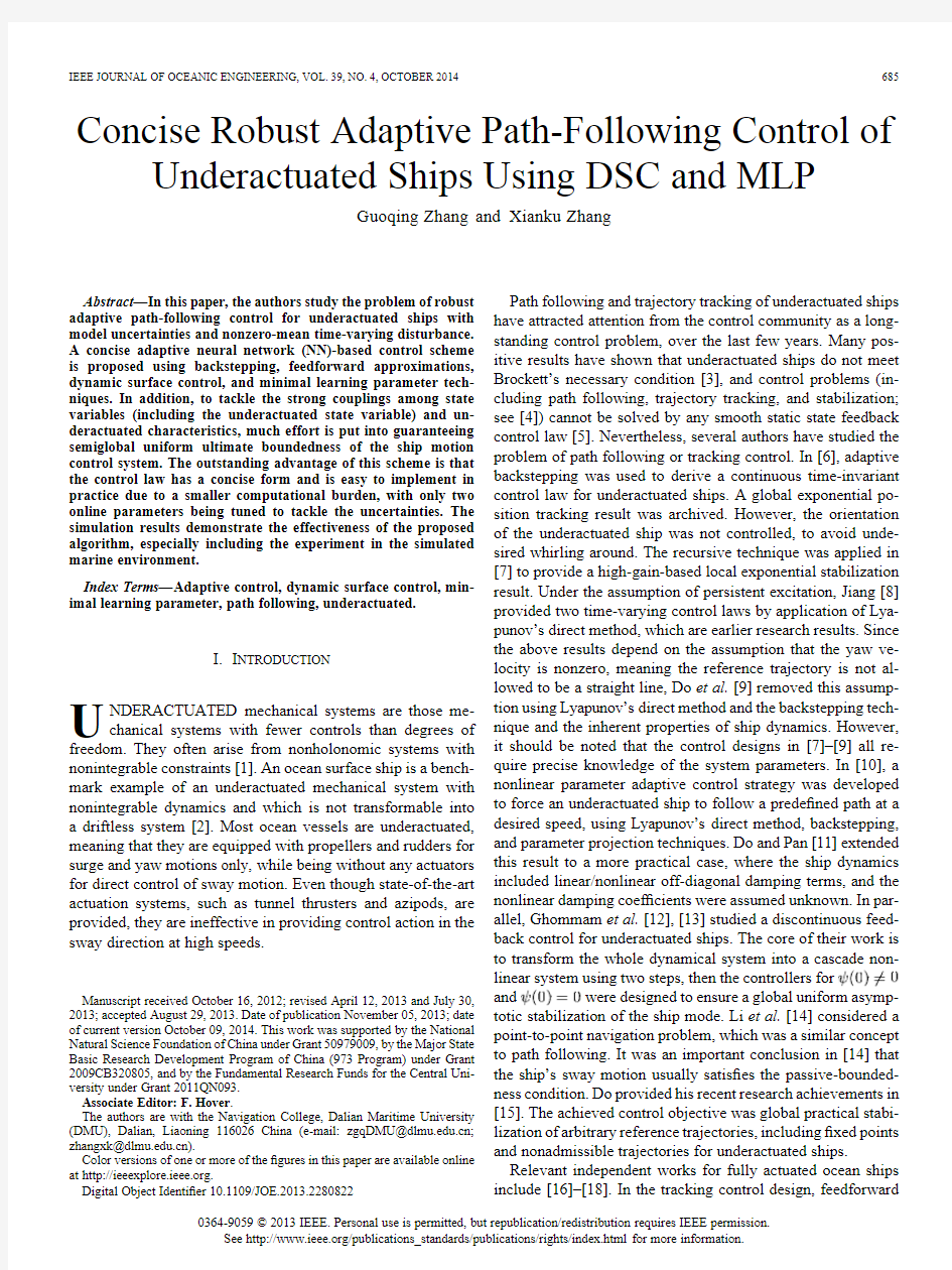
In marine navigation practice,the reference path is usually generated by waypoints with, which guide the vessel moving in the open sea[4].In this case, a novel route generating concept(Fig.1)is?rst introduced for underactuated ships by splitting the reference path into regular straight lines and smooth arcs,which can be generated by a vir-tual ship with order inputs and.To the best of the authors’knowledge,guidance systems for marine vessels have been de-tailed in[25].For the path following in the case of straight line paths,a line-of-sight(LOS)steering law is used to derive the de-sired heading angle,and then the control object can be guaranteed by a heading autopilot.However,few guidance laws are suited to the waypoint-based path generation for under-actuated ships in the current literature,and it is critical and im-portant for applying these theoretical path-following algorithms in the marine control engineering.
In Fig.1,the desired path of the virtual ship is
Two important input orders and are required to be derived for the task of path following.Normally,is a positive constant determined by the user,while is a order changing over time.In the straight lines and, .In the smooth arcs,is a nonzero constant that can be calculated for the virtual ship being without any inertia and uncertainties.
First,the angle of can be obtained from
(3) and the angle is de?
ned by.The turning radius,resting with in,is determined by interpolation in.If,.Fig.2.General framework of the ship’s path following.
Then,in arc can be easily obtained by .A similar procedure is employed repeatedly for each waypoint,and,?nally,the route generating is completed. Assumption2:Assume that the unstructured uncertainty terms satisfy, where,,and are unknown positive con-stants.
Assumption3:Assume that the sway velocity is passive bounded,following[14].
Remark2:The passive boundedness of the sway dynamic has been systematically analyzed considering different cases in [14].This assumption is easily satis?ed in the marine navigation practice.
Control objective:The control objective is to develop a concise robust adaptive path-following controller(design the surge force and the yaw moment)such that:1)all states of the underactuated ship are semiglobal uniformly ultimately bounded(SGUUB);and2)the underactuated surface ship(1) follows closely a virtual ship moving along a speci?ed path with a desired speed;see Fig.2.
B.NN-Based Function Approximation
RBF NNs are usually used as a tool for modeling nonlinear functions for their good capabilities in function approximation [26],[27].In this section,we introduce RBF NNs in the pro-posed control scheme to deal with arbitrary uncertainty.To use the MLP technique,Lemma1will be employed as follows. Lemma1[23],[28]:For any given real continuous function with,when the continuous function separation technique and the RBF NN approximation technique are used, can be written as follows:
(4) where is a vector of RBFs with the form of Gaussian functions
(5)
688IEEE JOURNAL OF OCEANIC ENGINEERING,VOL.39,NO.4,OCTOBER2014 is the approximation error with unknown upper bound,is
the node number of NNs,is the dimension number of,and
.. ...
.
..
.
..
.
is an optimal weight matrix.
III.D ESIGN OF THE C ONCISE A DAPTIVE NN
P ATH-F OLLOWING C ONTROL
Motivated by the ideas of the DSC and MLP techniques[19], [23],we develop a concise adaptive NN controller for an under-actuated ship(1)under Assumptions1–3.The control design procedure consists of two steps:for kinematic control and for kinetic control.First,we assume and are given immediate control signals.Then,the surge force and the yaw moment will be derived.The stability of the closed-loop system will then be discussed in Section III-B.
A.Control Design
Step1:Referring to Fig.2,we de?ne the following error vari-ables:
(6)
is the target position generated by a virtual ship.Note that is the ship’s azimuth angle relative to the virtual ship,and not yaw angle of the virtual ship,which is calculated by
(7) From Fig.2,it is easy to get
(8) Combining(1),(6),and(8),and differentiating with respect to and,we get
(9) Choose and as the virtual controls of and,i.e.,
(10) where and are design parameters.
To avoid redifferentiating the virtual controls in the next step, which leads to the so-called“explosion of complexity,”the DSC technique[20],[29],[30]is employed here.We introduce two ?rst-order?lters and,and let the virtual controls pass through them with time constants and,respectively
(11) Let and and,then
(12)
(13) From(10)and(11)
(14) where are continuous functions.
Remark3:For(10),note that the virtual control is not de?ned at,thus,we?rst assume in the control design that,and use
(15) to guarantee the assumption is satis?ed.
In(10),is a small positive value.introduced in is able to ensure that the real ship usually follows behind the virtual ship,which will facilitate satisfying condition and that the error variable satis?es. In Section IV,we select.
Step2:At this step,taking the time derivative of along (1)and(13),we obtain
(16)
ZHANG AND ZHANG:CONCISE ROBUST ADAPTIVE PATH-FOLLOWING CONTROL OF UNDERACTUATED SHIPS USING DSC AND MLP689
As are unknown smooth functions,they can be approximated by NNs as(4)
(17) where
Based on(17),the dynamic of the errors system(16)is given by
(18) with
(19) where is an unknown positive constant
Then
and
Similar to the previous discussion,we can get
(20) where
and
is an unknown positive constant. The corresponding control law and the parameters’update laws are taken to be
(21)
(22)where
and and are positive constants.
is the estimate of,and is the initial value of. Remark4:It can be observed that the form of the control law (21)is concise and easy to implement in ship engineering.i) The idea of adaptive neural control based on NN approximation guarantees that the controller is able to tackle arbitrary uncer-tainty of underactuated ships.ii)Even though there exist many nodes included in the RBF NNs and the systems include two in-puts,only two learning parameters need to be tuned on-line in the closed-loop system for the MLP technique(22).Com-bining with the DSC technique developed in[30],both problems of“explosion of complexity”and“curse of dimensionality”are circumvented simultaneously.That is the key to applying the theoretical result in practice.
In addition,the NNs are only used to tackle the unknown system functions[see(18)].The unknown control gain coef?-cients are not required to be estimated.Thus,the potential control singularity problem is avoided,which usually exists in many feedback linearization adaptive controls[31].
B.Main Result
Based on the above controller design,we have the main result stated as follows.
Theorem1:Consider the closed-loop system consisting of the underactuated ship(1)satisfying Assumptions1–3,the con-cise adaptive controller(21),and the MLP-based adaptive law (22).For all initial conditions satisfying
with any,one can tune the controller parameters, ,,,,,,,,,,and,such that all the signals in the closed-loop system are SGUUB.
Proof:Construct the Lyapunov function candidate
(23) For any and,the sets
are compact in,respectively,and
690IEEE JOURNAL OF OCEANIC ENGINEERING,VOL.39,NO.4,OCTOBER2014 is also compact in.Therefore,there exist positive constants
and such that.
The time derivative along(9),(10),(14),(18),(21),and
(22)is derived
(24) where is a small positive constant.From Young’s inequality, we have
(25)
(26) Noting the de?nition of,we have
..
.
(27)
Using the control law(21)and the adaptive law(22),(24) yields
(28) where
Note that,,,and are all control design parame-ters.Now we can choose
(29) with being positive constants.Finally,(28)be-comes
(30) where.By integration of(30),one has
(31) Based on the closed-loop gain shaping algorithm[32],is bounded by.Since are all con-stants,it is concluded that the signals are all bounded.In addition,Assumption3is satis?ed;see[10]and [14]for more details.Therefore,all the signals in the closed-loop system are SGUUB.
IV.S IMULATION R ESULTS
In this section,simulation results will be presented to verify the performance of the proposed control scheme.For this pur-pose,we consider the underactuated ship(length of38m,mass of11810kg),which has been considered in[14]and[33]. The results of two simulations are given here.In Section IV-A,it is interesting to compare the concise robust adaptive controller
ZHANG AND ZHANG:CONCISE ROBUST ADAPTIVE PATH-FOLLOWING CONTROL OF UNDERACTUATED SHIPS USING DSC AND MLP
691
Fig.3.Signal ?ow chart for
simulation.
Fig.4.Path-following trajectory in the 2-D plane:the proposed control scheme (dashed–dotten line)and the scheme in [14](dashed line).
with the result in [14],where the disturbances are constructed
by superposing the sine signals with different frequency.In Section IV-B,it is demonstrated how the proposed algorithm can perform in the marine practical https://www.doczj.com/doc/4419156441.html,parative Experiment
In the simulation,the proposed concise robust adaptive con-troller is compared with the result in [14].12010kg,
177.910kg,and 63610kg.The time-varying disturbances in the plant are
The reader is referred to [14]for the corresponding control pa-rameters.
The initial conditions are chosen as in (32).The reference path is generated by a virtual ship (2). 6.0m/s,and
0s 30s 30s
70s 70s
180
s
The concise adaptive controller in (10),(21),and (22)is implemented for the path-following control.Fig.3shows the
Fig.5.Position and orientation errors:the proposed control scheme (solid line)and the scheme in [14](dashed line).
signal ?ow chart for the simulation.The marked numbers denote formulas involved in the relative block.
For the concise robust adaptive controller,the control param-eters are taken as in (33).The RBF NNs for and include 25nodes,,with centers spaced in [10m/s,10m/s]for and [ 2.5rad/s,2.5rad/s]for and widths
(32)
(33)
The comparative results are shown in Figs.4–7.Fig.4
demonstrates the path-following trajectory,where the refer-ence path consists of a straight line and a circle,and it shows that despite the existence of the nonzero-mean time-varying disturbances and unknown model parameters,both the path-fol-lowing control with the proposed algorithm and the result in [14]are well established.Fig.6shows that the control efforts with the surge force are bounded within 0 5.210N,and the yaw moment is bounded within 8.510N m [4].In Fig.7,we can see that the adaptive parameters and are regulated rapidly to a reasonable range at 18s.In addition,note that the coordinates in Fig.7are a local zoom of the curves between 20and 180s.
In fact,the hardware of autopilot onboard is an industrial per-sonal computer (IPC,i.e.,controller).It is actually a computer suited to run in marine engineering.Based on the consideration,Table I gives the held computer memory and the elapsed time when the above digital simulation experiments are conducted
692IEEE JOURNAL OF OCEANIC ENGINEERING,VOL.39,NO.4,OCTOBER
2014
Fig.6.Control efforts:the proposed control scheme (solid line)and the scheme in [14](dashed
line).
Fig.7.Adaptive adjusting parameters
and
for the proposed scheme.
using the proposed control scheme and the one in [14].It is ob-vious that the burdensome computation of the algorithm can be alleviated effectively.
The results of the comparative performance experiment show that the concise robust adaptive path-following controller has much better performance in comparison with the existing algo-rithm.Note that,although the error in Fig.5is larger during the stage of the curve following,it is better from the overall viewpoint and the marine practice.
Remark 5:Fig.6shows that there exists an evident oscil-lating orientation error (see Fig.5)during the initial period of using the proposed controller due to the large tracking error and
TABLE I
C ALCULATIONS OF C OMPUTING B URDEN FOR THE P ROPOSED
C ONTROL S CHEME AN
D TH
E O NE IN
[14]
Fig.8.Graph of wind-generated waves with the sixth-level sea state.
the lack of knowledge about the plant nonlinearities.Note that this phenomenon is very common in universal adaptive path-following control schemes,i.e.,[11],[13],[14],[17],[34],and [35].However,in normal ship steering,it often moves ?rst close to the reference path by manual operation,and then switches the autopilot to the automatic mode.In addition,the lack of knowl-edge about the plant nonlinearities can be lessened by of ?ine training of the NNs to the unknown nonlinearities in advance.
B.Path-Following Control in Marine Environment
In this section,the marine navigation practice is con-sidered.The reference path is generated by ?ve way-points:
.The environmental disturbances include wind,
irregular wind-generated wave,and ocean currents.Refer to [24]and [25]for details.
In the simulation,the wind speed (beaufort 6)12.25m/s,and the wind direction (going from)165.The corresponding wind-generated wave is shown in Fig.8.The current speed 1.0m/s,and the current direction (going to)60.The other parameters (e.g.,the initial conditions and the control parameters)are set along with Section IV-A.Figs.9–11illustrate simulation results of the path-following control in the marine environment.From Fig.9,
ZHANG AND ZHANG:CONCISE ROBUST ADAPTIVE PATH-FOLLOWING CONTROL OF UNDERACTUATED SHIPS USING DSC AND MLP
693
Fig.9.Path-following trajectory (2-D)in the marine
environment.
Fig.10.Control efforts with the sixth-level sea state.
the ship successfully tracks the waypoint-generated reference path and the autoturn in each waypoint.Fig.10presents the control efforts in the marine environment,which are within a reasonable range.It is noted that the drawn chatter may not be realistic for the vessel.In fact,the mathematical model (1)is simpli ?ed without modules to describe the marine main engine and the rudder servo machine.Those are the main factors to cause chattering,since the rudder servo system has the ?ltering effectiveness from the rudder angle to the yaw moment.Thus,the phenomenon would not appear in the marine control engi-neering.Based on the above analysis,the simulation has shown the good performance of the proposed concise control
scheme.
Fig.11.Adaptive adjusting parameters and in the marine environment.
V .C ONCLUSION
This paper presented the development of a concise adaptive NN path-following controller for underactuated ships with unknown parameters and nonzero-mean time-varying https://www.doczj.com/doc/4419156441.html,pared with the existing results,the proposed scheme obtains some advantages:a concise form and an ease of implementation,due to its smaller computational burden.The problems of the “explosion of complexity”and the “curse of dimensionality”are circumvented by a fusion of the DSC technique.The stability of the closed-loop system has been proven using the Lyapunov theory.Simulation results have been presented to demonstrate the effectiveness of the novel controller.
However,this work naturally cannot attend to every detail of the control design.We are working on an extension of our proposed scheme to the following problems.Results on these topics will be reported elsewhere.
?Control input hysteresis nonlinearity:control hysteresis is one of the most important nonsmooth nonlinearities which need to be considered in practical applications.
?Adaptive output feedback:in this case,the model parame-ters of the underactuated ships are unknown and only the surge,sway,and yaw displacements are available for feed-back.
A CKNOWLEDGMENT
The authors would like to thank the anonymous reviewers for their valuable comments and suggestions that improved the quality of this paper.
R EFERENCES
[1]Z.-P.Jiang,“Controlling underactuated mechanical systems:A review
and open problems,”in Advances in the Theory of Control,Signals and Systems with Physical Modeling ,ser.Lecture Notes in Control and Information Sciences.Berlin,Germany:Springer-Verlag,2011,vol.407,pp.77–88.
694IEEE JOURNAL OF OCEANIC ENGINEERING,VOL.39,NO.4,OCTOBER2014
[2]K.Y.Wichlund,O.J.Sordalen,and O.Egeland,“Control properties of
underactuated vehicles,”in Proc.IEEE Int.Conf.Robot.Autom.,1995, pp.2009–2014.
[3]R.Brockett,https://www.doczj.com/doc/4419156441.html,lman,and H.Sussman,Differential Geometric Con-
trol Theory.Boston,MA,USA:Birkhauser,1983,ch.3.
[4]K.D.Do and J.Pan,Control of Ships and Underwater Vehicles.New
York,NY,USA:Springer-Verlag,2009,pp.39–54.
[5]W.Dong and Y.Guo,“Global time-varying stabilization of underac-
tuated surface vessel,”IEEE Trans.Autom.Control,vol.50,no.6,pp.
859–864,Jun.2005.
[6]J.-M.Godhavn,T.I.Fossen,and S.P.Berge,“Nonlinear and adaptive
backstepping designs for tracking control of ships,”Int.J.Adaptive Control Signal Process.,vol.12,pp.649–668,1998.
[7]K.Y.Pettersen and H.Nijmeijer,“Underactuated ship tracking con-
trol:Theory and experiments,”Int.J.Control,vol.74,no.14,pp.
1435–1446,2001.
[8]Z.-P.Jiang,“Global tracking control of underactuated ships by Lya-
punov’s direct method,”Automatica,vol.38,pp.301–309,2002. [9]K.D.Do,Z.P.Jiang,and J.Pan,“Underactuated ship global tracking
under relaxed conditions,”IEEE Trans.Autom.Control,vol.47,no.9, pp.1529–1535,Sep.2002.
[10]K.D.Do,Z.P.Jiang,and J.Pan,“Robust adaptive path following of
underactuated ships,”Automatica,vol.40,pp.929–944,2004. [11]K.D.Do and J.Pan,“Global robust adaptive path following of under-
actuated ships,”Automatica,vol.42,pp.1713–1722,2006.
[12]J.Ghommam,F.Mnif,A.Benali,and N.Derbel,“Asymptotic back-
stepping stabilization of an underactuated surface vessel,”IEEE Trans.
Control Syst.Technol.,vol.14,no.6,pp.1150–1157,Nov.2006. [13]J.Ghommam,F.Mnif,and N.Derbel,“Global stabilisation and
tracking control of underactuated surface vessels,”IET Control Theory Appl.,vol.4,no.1,pp.71–88,2010.
[14]J.-H.Li,P.-M.Lee,B.-H.Jun,and Y.-K.Lim,“Point-to-point navi-
gation of underactuated ships,”Automatica,vol.44,pp.3201–3205, 2008.
[15]K.D.Do,“Practical control of underactuated ships,”Ocean Eng.,vol.
37,pp.1111–1119,2010.
[16]K.P.Tee and S.S.Ge,“Control of fully actuated ocean surface vessels
using a class of feedforward approximators,”IEEE Trans.Control Syst.
Technol.,vol.14,no.4,pp.750–756,Jul.2006.
[17]M.Chen,S.S.Ge,and Y.S.Choo,“Neural network tracking control of
ocean surface vessels with input saturation,”in Proc.IEEE Int.Conf.
Autom.Logistics,Shenyang,China,Aug.2009,pp.85–89.
[18]M.Chen,S.S.Ge,and R.Cui,“Adaptive NN tracking control of over-
actuated ocean surface vessels,”in Proc.8th World Congr.Intell.Con-trol Autom.,Jinan,China,Jul.2010,pp.548–552.
[19]M.Krstic,I.Kanellakopoulos,and P.Kokotovic,Nonlinear and Adap-
tive Control Design.New York,NY,USA:Wiley,1995,ch.2–4. [20]S.S.Ge and C.Wang,“Direct adaptive NN control of a class of non-
linear systems,”IEEE Trans.Neural Netw.,vol.13,no.1,pp.214–221, Jan.2002.
[21]T.-S.Li,D.Wang,G.Feng,and S.-C.Tong,“A DSC approach to robust
adaptive NN tracking control for strict-feedback nonlinear systems,”
IEEE Trans.Syst.Man Cybern.B,Cybern.,vol.40,no.3,pp.915–927, Jun.2010.
[22]Y.Yang and X.Wang,“Adaptive NN tracking control for a class of un-
certain nonlinear systems using radial-basis-function neural networks,”
Neurocomputing,vol.70,pp.932–941,2007.
[23]T.-S.Li,R.-H.Li,and D.Wang,“Adaptive neural control of nonlinear
MIMO systems with unknown time delays,”Neurocomputing,vol.78, pp.83–88,2012.
[24]T.I.Fossen,Guidance and Control of Ocean Vehicles.New York,
NY,USA:Wiley,1998,pp.48–54.
[25]T.I.Fossen,Handbook of Marine Craft Hydrodynamics and Motion
Control.New York,NY,USA:Wiley,2011,pp.241–278.
[26]M.M.Polycarpou,“Stable adaptive neural control scheme for non-
linear systems,”IEEE Trans.Autom.Control,vol.41,no.3,pp.
447–450,May1996.
[27]M.M.Polycarpou and M.J.Mears,“Stable adaptive tracking of uncer-
tain systems using nonlinearly parameterized on-line approximators,”
Int.J.Control,vol.70,no.3,pp.363–384,1998.
[28]Y.Yang and C.Zhou,“Robust adaptive fuzzy tracking control for a
class of perturbed strict-feedback nonlinear systems via small-gain ap-
proach,”Inf.Sci.,vol.170,pp.211–234,2005.
[29]P.P.Yip and J.K.Hedrick,“Adaptive dynamic surface control:A sim-
pli?ed algorithm for adaptive backstepping control of nonlinear sys-
tems,”Int.J.Control,vol.71,no.5,pp.959–979,1998.
[30]D.Wang and J.Huang,“Neural network-based adaptive dynamic sur-
face control for a class of uncertain nonlinear systems in strict-feed-
back form,”IEEE Trans.Neural Netw.,vol.16,no.1,pp.195–202,
Jan.2005.
[31]S.S.Ge,C.C.Hang,T.H.Lee,and T.Zhang,Stable Adaptive Neural
Network Control.Norwell,MA,USA:Kluwer,2001,pp.2–8.
[32]X.Zhang,Ship Motion Concise Robust Control.Beijing,China:Sci-
ence Press,2012,pp.35–40.
[33]K.D.Do and J.Pan,“Underactuated ships follow smooth paths with in-
tegral actions and without velocity measurements for feedback:Theory
and experiments,”IEEE Trans.Control Syst.Technol.,vol.14,no.2,
pp.308–322,Mar.2006.
[34]W.Meng,C.Guo,and Y.Liu,“Robust adaptive path following for
underactuated surface vessels with uncertain dynamics,”J.Mar.Sci.
Appl.,vol.11,pp.244–250,2012.
[35]Z.Peng,D.Wang,and X.Hu,“Robust adaptive formation control of
underactuated autonomous surface vehicles with uncertain dynamics,”
IET Control Theory Appl.,vol.5,no.12,pp.1378–1387,
2010.
Guoqing Zhang received the B.Sc.and M.Sc.de-
grees from the Navigation College,Dalian Maritime
University(DMU),Dalian,China,in2010and2012,
where he is currently working toward the Ph.D.de-
gree in the area of modeling and control of marine
vehicles.
His current research interests include adaptive
control,nonlinear control,and their application on
the marine control
system.
Xianku Zhang received the Ph.D.degree from
Dalian Maritime University(DMU),Dalian,China,
in1998.
Currently,he is a Professor/Doctor Supervisor at
DMU.He is a scholarship leader of a national key
discipline named traf?c information engineering and
control,and Vice Institute Director of Marine Sim-
ulation and Control.He authored or coauthored105
papers,among which?ve papers are referred by the
Science Citation Index and46papers are referred by
the Engineering Index,and11books in the?elds of ship motion control,robust control,intelligent control,and computer program-ming.His current research areas are robust control,intelligent control,and their application on the marine control system.
Prof.Zhang received one second-class scienti?c award in China and two second-class scienti?c awards from Liaoning Province,China.
鲁棒控制理论中的H∞控制理论 (浙江大学宁波理工学院信息科学与工程分院自动化) 【摘要】首先简要的介绍了鲁棒控制中的H∞控制理论,并把其发展分为两个阶段,而后就上当已存在的H∞控制的主要成果进行了讨论和归纳,还指出了H∞控制理论尚未解决的问题。 【关键词】H∞控制理论;非线性系统;时滞;范数 1.概述 鲁棒控制(Robust Control)方面的研究始于20世纪50年代。在过去的20年中,鲁棒控制一直是国际自控界的研究热点。所谓鲁棒性,是指标称系统所具有的某一种性能品质对于具有不确定性的系统集的所有成员均成立,如果所关心的是系统的稳定性,那么就称该系统具有鲁棒稳定性;如果所关心的是用干扰抑制性能或用其他性能准则来描述的品质,那么就称该系统具有鲁棒性能。主要的鲁棒控制理论有:Kharitonov区间理论;H∞控制理论;结构奇异值理论u理论; 鲁棒控制理论是分析和处理具有不确定性系统的控制理论,包括两大类问题:鲁棒性分析及鲁棒性综合问题。鲁棒性分析是根据给定的标称系统和不确定性集合,找出保证系统鲁棒性所需的条件;而鲁棒性综合(鲁棒控制器设计问题)就是根据给定的标称模型和不确定性集合,基于鲁棒性分析得到的结果来设计一个控制器,使得闭环系统满足期望的性能要求。 2.H∞控制理论出现的背景及意义 1981年,加拿大著名学者Zames在其论文中引入了H∞范数作为目标函数进行优化设计,标志着H∞控制理论的诞生。Zames考虑了这样一个单入单出( SISO)系统的设计问题: 假设干扰信号属于某一有限能量的已知信号集,要求设计一个反馈控制器,使闭环系统稳定,且干扰对系统的影响最小。要解决这样的问题就必须在能够使闭环系统稳定的所有控制器中选出一个控制器使之相应的灵敏度函数的H∞范数最小。 虽然Zames 首先提出了H∞最优化问题,但是他没能给出行之有效的解法。
非线性系统的鲁棒自适应控制 Robust Adaptive Control of Uncertain Nonlinear Systems 郝仁剑3120120359 摘要:本文以非线性系统的控制问题为背景,介绍了多种经典的非线性系统的控制方法以及研究进展,分析了各种控制方法存在的优点和不足。着重介绍了鲁棒自适应控制在非线性系统中的应用,结合该领域的近期研究进展和实际应用背景,给出对鲁棒自适应控制的进一步研究目标。 关键词:非线性系统鲁棒控制自适应控制 1.前言 任何实际系统都具有非线性特性,非线性现象无处不在。严格地说,线性特性只是其中的特例,但是非线性系统与线性系统又具有本质的区别。由于非线性系统不满足叠加原理,因此非线性特性千差万别,这也给非线性系统的研究带来了很大的困难。同时,对于非线性系统很难求得完整的解,一般只能对非线性系统的运动情况做出估计。众所周知,控制理论经历了经典控制理论和现代控制理论两个发展阶段。在第二次世界大战前后发展起来的经典控制理论应用拉普拉斯变换等工程数学工具来分析系统的品质。它广泛地应用于单输入单输出、线性、定常、集中参数系统的研究中。随着控制对象的日益复杂以及人们对控制系统精度的不断提高,经典控制理论的局限性就暴露出来了。在20世纪50年代,Bellman根据最优原理创立了动态规划。同时庞特里亚金等学者创立了最大值原理。后来,Kalman提出了一系列重要的概念,如可观性,可控性,最优线性二次状态反馈,Kalman滤波等。这些理论和概念的提出大大促进了现代控制理论的发展。控制系统的设计都需要以被控对象的数学模型为依据,然而对于任何被控对象不可能得到其精确的数学模型,如在建立机器人的数学模型时,需要做一些合理的假设,而忽略一些不确定因数。不确定性的必然存在也正促使了现代控制理论中另一重要的研究领域——鲁棒控制理论的发展。Zmaes关于小增益定理的研究以及Kalman关于单输入单输出系统LQ调节器稳定裕量的分析为鲁棒控制理论的发展产生了重要的影响。特别是Zmaes1981年发表的论文[1]标志H∞控制理论的起步。1984年Francis和Zmaes基于古典插值理论提出H∞问题的初步解法。Glover运用Hankel算子理论给出了H∞问题的解析解。Doyle在状态空间上对Glover解法进行整理和归纳。至此H∞控制理论体系初步形成。同时,Doyle首次提出结构化奇异值的概念,后来形成了μ解析理论。另外一种重要的控制器设计方法是基于Lyapunov函数的方法。在进行鲁棒控制器的设计时,一般都假设系统的不确定性属于一个可描述集,比如增益有界,且上界己知等。一般来说,鲁棒控制是比较保守的控制策略。对所考虑集合内的个别元素,该系统并不是最佳控制。对于具有参数不确定性的一类系统,自适应控制技术被提了出来,如模型参考自适应控制和自校正控制等。在实际应用中,由于被控对象具有未建模动态,过程噪声或扰动的统计特性远比设计时所设想的情况更复杂,以及持续激励条件和严正实条件等“理想条件”被打破,这都会导致自适应控制算法的失稳。于是自适应控制的鲁棒性课题,即鲁棒自适应控制受到了广泛的关注。大量的工程实践表明,对于复杂的工业对象和过程,引入自适应策略能够提高控制精度,提高生产效率,降低成本。近年来,非线性自适应控制技术取得突破性的发展,控制器的结构化设计技术也正日益得到广泛的研究与应用。
Lyapunov Lyapunov稳定性理论概述稳定性理论概述稳定性理论概述 稳定性理论是19 世纪80 年代由俄国数学家Lyapunov创建的,它在自动控制、航空技术、生态生物、生化反应等自然科学和工程技术等方面有着广泛的应用,其概念和理念也发展得十分迅速。通过本学期“力学中的数学方法”课程的学习,我对此理论的概况有了一些认识和体会,总结于本文中。 一, 稳定性的概念稳定性的概念 初始值的微分变化对不同系统的影响不同,例如初始值问题 ax dt dx = , x(0)=x 0 , t≥0,x 0≥0 (1) 的解为e x at t x 0 )(= ,而x=0 是(1)式的一个解。当a f 0时,无论|x 0|多小,只要 |x 0| ≠ 0 ,在t→+∞时,总有x(t)→ ∞,即初始值的微小变化会导致解的误差任意大,而当a ?0时,e x at t x 0 )(= 。与零解的误差不会超过初始误差x 0,且随 着t 值的增加很快就会消失,所以,当|x 0|很小时,x(t)与零解的误差也很小。 这个例子表明a f 0时的零解是“稳定”的。下面,我们就给出微分方程零解稳定的严格定义。 设微分方程 ),(x t f dt dx =, x(t 0)=x 0 , x ∈R n (2) 满足解存在唯一定理的条件,其解x(t)=x(t,t 0,x 0)的存在区间是),(+∞?∞,f(t,x)还满足条件: f (t ,0)=0 (3) (3)式保证了x(t) = 0 是(2)式的解,我们称它为零解。 这里给出定义1:若对任意给定的ε > 0,都能找到δ=δ(ε,t 0),使得当||x 0||<δ时的解满足x ( t,x 0 , x 0 ) || x ( t, t 0 , x 0 ) || <ε, t ≥ t 0 , 则称(2)式的零解是稳定的,否则称(2)式的零解是不稳定的。
鲁棒控制设计报告 学院 专业 报告人
目录 1 绪论 (2) 1.1控制系统设计背景 (2) 1.2本文主要工作分配 (3) 2 一级倒立摆模型建立 (4) 2.1一级倒立摆的工作原理 (4) 2.2一级倒立摆的数学模型 (4) 3 H∞鲁棒控制器设计 (6) 3.1基于Riccati方程的H∞控制 (7) 3.2基于LMI的H∞控制 (7) 4 一级倒立摆系统的仿真 (9) 4.1一级倒立摆控制系统设计 (9) 4.2闭环控制系统仿真及分析 (10) 5 结论 (13)
1 绪论 1.1控制系统设计背景 一级倒立摆系统是一个典型非线性多变量不稳定系统,在研究火箭箭身的姿态稳定控制、机器人多自由度运动稳定设计、直升机飞行控制等多种领域中得到了广泛的应用,因此以倒立摆作为被控对象进行控制方法的研究具有重要的现实意义。为解决一级倒立摆系统的非线性、强耦合、多变量、自然不稳定问题,本文利用H∞鲁棒控制实现对一级倒立摆的控制。 Mg 图1.1 一级倒立摆系统结构图 本文采用的直线一级倒立摆的基本系统如图1.1所示,它是由沿直线导轨运动的小车以及一端固定于小车上的材质均匀的摆杆组成,它是一个不稳定的系统,当倒立摆出出现偏角θ后,如果不给小车施加控制力,倒立摆会倾倒。所以本文采用H∞鲁棒控制方法的目的是通过调节水平力F的大小控制小车的运动,使倒立摆处于竖立的垂直位置。控制指标为:倒立摆系统的从初始状态调节到小车停留在零点、并使摆杆的摆角为0的稳定状态。
1.2本文主要工作分配 第一章:对一级倒立摆系统的特点、结构以及控制要求进行阐述。 第二章:根据一级倒立摆的结构,利用机理建模法建立被控对象的精确数学模型,并在系统平衡点处进行线性化,得到系统简化的状态方程。 第三章:首先H∞鲁棒控制的基本原理,然后分别利用Riccati方程和LMI 方法设计H∞状态反馈控制器。 第四章:首先使用MATLAB计算基于Riccati方程的H∞状态反馈控制器和基于LMI的H∞状态反馈控制器,然后进行闭环控制系统的仿真并控制系统的性能分析。 第五章:对本次设计进行总结。
自适应PID控制 摘要:自适应PID控制是一门发展得十分活跃控制理论与技术,是自适应控制理论的一个重要组成部分,本文简要回顾PID控制器的发展历程,对自适应PID控制的主要分支进行归类,介绍和评述了一些有代表性的算法。 关键词:PID控制,自适应,模糊控制,遗传算法。 Abstract: The adaptive PID control is a very active developed control theory and technology and is an important part of adaptive control theory.This paper briefly reviews the development process PID controller.For adaptive PID control of the main branches, the paper classifies,introduces and reviews some representative algorithms. Keywords: PID control, adaptive, fuzzy control, genetic algorithm 1 引言 从问世至今已历经半个世纪的PID控制器广泛地应用于冶金、机械、化工、热工、轻工、电化等工业过程控制之中,PID控制也是迄今为止最通用的控制方法, PID控制是最早发展起来的控制策略之一,因为他所涉及的设计算法和控制结构都很简单,并且十分适用于工程应用背景,所以工业界实际应用中PID 控制器是应用最广泛的一种控制策略(至今在全世界过程控制中用的80% 以上仍是纯PID调节器,若改进型包含在内则超过90%)。由于实际工业生产过程往往具有非线性和时变不确定性,应用常规PID控制器不能达到理想控制效果,长期以来人们一直寻求PID控制器参数的自动整定技术,以适应复杂的工况和高指标的控制要求。随着微机处理技术和现代控制理论诸如自适应控制、最优控制、预测控制、鲁棒控制、智能控制等控制策略引入到PID控制中,出现了许多新型PID控制器。人们把专家系统、模糊控制、神经网络等理论整合到PID控制器中,这样既保持了PID控制器的结构简单、适用性强和整定方便等优点,又通过先进控制技术在线调整PID控制器的参数,以适应被控对象特性的变化。 2 自适应PID控制概念及发展 2.1 PID控制器 常规PID控制系统原理框图如下图所示,系统由模拟PID控制器和被控对象组成。
【总结】 Lyapunov指数的计算方法非线性理论 近期为了把计算LE的一些问题弄清楚,看了有7~9本书!下面以吕金虎《混沌时间序列分析及其应用》、马军海《复杂非线性系统的重构技术》为主线,把目前已有的LE计算方法做一个汇总! 1. 关于连续系统Lyapunov指数的计算方法连续系统LE的计算方法主要有定义方法、Jacobian方法、QR分解方法、奇异值分解方法,或者通过求解系统的微分方程,得到微分方程解的时间序列,然后利用时间序列(即离散系统)的LE求解方法来计算得到。关于连续系统LE的计算,主要以定义方法、Jacobian方法做主要介绍容。 (1)定义法
定义法求解Lyapunov指数.JPG 关于定义法求解的程序,和matlab板块的“连续系统LE求解程序”差不多。以Rossler系统为例 Rossler系统微分方程定义程序 function dX = Rossler_ly(t,X) %Rossler吸引子,用来计算Lyapunov指数 %a=0.15,b=0.20,c=10.0 %dx/dt = -y-z, %dy/dt = x+ay, %dz/dt = b+z(x-c), a = 0.15; b = 0.20; c = 10.0; x=X(1); y=X(2); z=X(3); % Y的三个列向量为相互正交的单位向量 Y = [X(4), X(7), X(10); X(5), X(8), X(11);
X(6), X(9), X(12)]; % 输出向量的初始化,必不可少 dX = zeros(12,1); % Rossler吸引子 dX(1) = -y-z; dX(2) = x+a*y; dX(3) = b+z*(x-c); % Rossler吸引子的Jacobi矩阵 Jaco = [0 -1 -1; 1 a 0; z 0x-c]; dX(4:12) = Jaco*Y; 求解LE代码: % 计算Rossler吸引子的Lyapunov指数clear; yinit = [1,1,1]; orthmatrix = [1 0 0; 0 1 0; 0 0 1]; a = 0.15; b = 0.20; c = 10.0; y = zeros(12,1); % 初始化输入 y(1:3) = yinit; y(4:12) = orthmatrix; tstart = 0; % 时间初始值 tstep = 1e-3; % 时间步长 wholetimes = 1e5; % 总的循环次数 steps = 10; % 每次演化的步数 iteratetimes = wholetimes/steps; % 演化的次数mod = zeros(3,1); lp = zeros(3,1); % 初始化三个Lyapunov指数 Lyapunov1 = zeros(iteratetimes,1); Lyapunov2 = zeros(iteratetimes,1); Lyapunov3 = zeros(iteratetimes,1); for i=1:iteratetimes
鲁棒控制理论综述 作者学号: 摘要:本文首先介绍鲁棒控制理论涉及的两个基本概念(不确定性和鲁棒)和发展过程,然 H控制理论,最后指出鲁棒控制研后叙述鲁棒控制理论中两种主要研究方法:μ理论、∞ 究的问题和扩展方向。 H控制理论 关键词:鲁棒控制理论,μ理论,∞ 一、引言 自从系统控制(Systems and Control)作为一门独立的学科出现,对于系统鲁棒性的研究也就出现了。这是由这门学科的特色和研究对象决定的。对于世界上的任何系统。由于系统本身复杂性或是人们对其认识的不全面,在系统建立模型时,很难用数学语言完全描述刻画。在这样的背景下,鲁棒性的研究也就自然而然地出现了。 二、不确定性与鲁棒 1、不确定性 谈到系统的鲁棒性,必然会涉及系统的不确定性。由于控制系统的控制性能在很大程度上取决于所建立的系统模型的精确性,然而,由于种种原因实际被控对象与所建立的模型之间总存在着一定的差异,这种差异就是控制系统设计所面临的不确定性。这种不确定性通常分为两类:系统内部的不确定性和系统外部的不确定性。这样,就需要一种能克服不确定性影响的控制系统设计理论。这就是鲁棒控制所要研究的课题。 2、鲁棒 “鲁棒”一词来自英文单词“robust”的音译,其含义是“强壮”或“强健”。所谓鲁棒性(robustness),是指一个反馈控制系统在某一特定的不确定性条件下具有使稳定性、渐近调节和动态特性这三方面保持不变的特性,即这一反馈控制系统具有承受这一类不确定性的能力。具有鲁棒性的控制系统称为鲁棒控制系统。在工程实际控制问题中,系统的不确定性一般是有界的,在鲁棒控制系统的设计中,先假定不确定性是在一个可能的范围内变化,然后在这个可能的变化范围内进行控制器设计。鲁棒控制系统设计的思想是:在掌握不确定性变化范围的前提下,在这个界限范围内进行最坏情况下的控制系统设计。因此,如果设计的控制系统在最坏的情况下具有鲁棒性,那么在其他情况下也具有鲁棒性。 三、发展历程 鲁棒控制系统设计思想最早可以追溯到1927年Black针对具有摄动的精确系统的大增益反馈设计。由于当时不知道反馈增益和控制系统稳定性之间的确切关系,所以设计出来的控制系统往往是动态不稳定的。早期的鲁棒研究主要集中在Bode图,1932年Nyquist提出了基于Nyquist曲线的频域稳定性判据,使得反馈增益和控制系统稳定性之间的关系明朗化。1945年Bode讨论了单输入单输出(SISO)反馈系统的鲁棒性,提出了利用幅值和相位稳定裕度来得到系统能容许的不确定范围。这些方法主要用于单输入单输出系统而且这些关于鲁棒控制的早期研究主要局限于系统的不确定性是微小的参数摄动情形,尚属灵敏度分析的范畴,从数学上说是无穷小分析思想,并且只是停留在理论上。20世纪六七十年代,鲁棒控制只是将SISO系统的灵敏度分析结果向MIMIO进行了初步的推广[1],与此同时,状态空间理论引入控制论后,系统控制取得了很大的发展,鲁棒问题也显得更加重要,其中就要提到两篇对现代鲁棒控制理论的建立有重要影响的文章:一篇是Zames在1963年关于小增益定理的论文[2],另一篇是1964年Kalman关于单入单输出系统LQ调节器稳定裕量分析的研究报告[3]。鲁棒控制这一术语第一次在论文中出现是在1971年Davion的论文[4],而首先将鲁棒控制写进论文标题的是Pearson等人于1974年发表的论文[5]。当然,鲁棒控制能够
【总结】Lyapunov指数的计算方法非线性理论 近期为了把计算LE的一些问题弄清楚,看了有7~9本书!下面以吕金虎《混沌时间序列分析及其应用》、马军海《复杂非线性系统的重构技术》为主线,把目前已有的LE计算方法做一个汇总! 1. 关于连续系统Lyapunov指数的计算方法连续系统LE的计算方法主要有定义方法、Jacobian方法、QR分解方法、奇异值分解方法,或者通过求解系统的微分方程,得到微分方程解的时间序列,然后利用时间序列(即离散系统)的LE求解方法来计算得到。关于连续系统LE的计算,主要以定义方法、Jacobian方法做主要介绍内容。 (1)定义法
定义法求解Lyapunov指数.JPG 关于定义法求解的程序,和matlab板块的“连续系统LE求解程序”差不多。以Rossler系统为例 Rossler系统微分方程定义程序 function dX = Rossler_ly(t,X) %Rossler吸引子,用来计算Lyapunov指数 %a=0.15,b=0.20,c=10.0 %dx/dt = -y-z, %dy/dt = x+ay, %dz/dt = b+z(x-c), a = 0.15; b = 0.20; c = 10.0; x=X(1); y=X(2); z=X(3); % Y的三个列向量为相互正交的单位向量 Y = [X(4), X(7), X(10); X(5), X(8), X(11); X(6), X(9), X(12)]; % 输出向量的初始化,必不可少 dX = zeros(12,1); % Rossler吸引子
dX(1) = -y-z; dX(2) = x+a*y; dX(3) = b+z*(x-c); % Rossler吸引子的Jacobi矩阵 Jaco = [0 -1 -1; 1 a 0; z 0x-c]; dX(4:12) = Jaco*Y; 求解LE代码: % 计算Rossler吸引子的Lyapunov指数 clear; yinit = [1,1,1]; orthmatrix = [1 0 0; 0 1 0; 0 0 1]; a = 0.15; b = 0.20; c = 10.0; y = zeros(12,1); % 初始化输入 y(1:3) = yinit; y(4:12) = orthmatrix; tstart = 0; % 时间初始值 tstep = 1e-3; % 时间步长 wholetimes = 1e5; % 总的循环次数 steps = 10; % 每次演化的步数 iteratetimes = wholetimes/steps; % 演化的次数mod = zeros(3,1); lp = zeros(3,1); % 初始化三个Lyapunov指数 Lyapunov1 = zeros(iteratetimes,1); Lyapunov2 = zeros(iteratetimes,1); Lyapunov3 = zeros(iteratetimes,1); for i=1:iteratetimes tspan = tstart:tstep:(tstart + tstep*steps); [T,Y] = ode45('Rossler_ly', tspan, y); % 取积分得到的最后一个时刻的值 y = Y(size(Y,1),:); % 重新定义起始时刻 tstart = tstart + tstep*steps;
对鲁棒控制的认识 姓名:赵呈涛 学号: 092030071 专业:双控
鲁棒控制(RobustControl)方面的研究始于20世纪50年代。在过去的20年中,鲁棒控制一直是国际自控界的研究热点。所谓“鲁棒性”,是指控制系统在一定(结构、大小)的参数摄动下,维持某些性能的特性。根据对性能的不同定义,可分为稳定鲁棒性和性能鲁棒性。如果所关心的是系统的稳定性,那么就称该系统具有鲁棒稳定性;如果所关心的是用干扰抑制性能或用其他性能准则来描述的品质,那么就称该系统具有鲁棒性能。以闭环系统的鲁棒性作为目标设计得到的固定控制器称为鲁棒控制器。 鲁棒控制的早期研究,主要针对单变量系统(SISO)的在微小摄动下的不确定性,具有代表性的是Zames提出的微分灵敏度分析。然而,实际工业过程中故障导致系统中参数的变化,这种变化是有界摄动而不是无穷小摄动,因此产生了以讨论参数在有界摄动下系统性能保持和控制为内容的现代鲁棒控制。现代鲁棒控制是一个着重控制算法可靠性研究的控制器设计方法,其设计目标是找到在实际环境中为保证安全要求控制系统最小必须满足的要求。一旦设计好这个控制器,它的参数不能改变而且控制性能能够保证。 鲁棒控制方法,是对时间域或频率域来说,一般要假设过程动态特性的信息和它的变化范围,一些算法不需要精确的过程模型,但需要一些离线辨识。鲁棒控制理论是分析和处理具有不确定性系统的控制理论,包括两大类问题:鲁棒性分析及鲁棒性综合问题。鲁棒性分析是根据给定的标称系统和不确定性集合,找出保证系统鲁棒性所需的条件;而鲁棒性综合(鲁棒控制器设计问题)就是根据给定的标称模型和不确定性集合,基于鲁棒性分析得到的结果来设计一个控制器,使得闭环系统满足期望的性能要求。主要的鲁棒控制理论有: (1)Kharitonov区间理论; 控制理论; (2)H ∞ (3)结构奇异值理论μ理论。 下面就这三种理论做简单的介绍。 1 Kharitonov区间理论 1.1参数不确定性系统的研究概况 对参数不确定性系统的研究源于20世纪20年代。Black采用大回路增益的反馈控制技术来抑制真空管放大器中存在的严重不确定性,由于采用大回路增益,所以设计的系
鲁棒控制综述 课程目标 1.了解鲁棒控制研究的基本问题 2.掌握鲁棒控制的基础知识和基本概念 3.明确鲁棒控制问题及其形式化描述 4.掌握几种鲁棒稳定性分析与设计方法 5.掌握状态空间H∞控制理论 6.了解鲁棒控制系统的μ分析与μ综合方法 7.初步了解非线性系统鲁棒控制方法 8.掌握时滞系统的鲁棒控制稳定性分析 控制系统就是使控制对象按照预期目标运行的系统。 大部分的控制系统是基于反馈原理来进行设计的 反馈控制已经广泛地应用于工业控制、航空航天和经济管理等各个领域。 不确定性 在实际控制问题中,不确定性是普遍存在的 所描述的控制对象的模型化误差 可能来自外界扰动 因此,控制系统设计必须考虑不确定性带来的影响。 控制系统设计的任务 对于给定的控制对象和传感器,寻找一个控制器,使反馈控制系统能够在实际工作环境中按预期目标运行 ●实际控制对象就是具体的装置、设备或生产过程 ●通过各种建模方法,可以建立实际控制对象的模型 ●针对控制对象的模型,应用控制理论提供的设计方法设计出控制器,对实际控制对 象实施控制 ●控制系统的控制效果在很大程度上取决于实际控制对象模型的准确性 ●在控制系统设计中采用的模型与实际控制对象存在着一定的差异,即存在着模型不 确定性 ●控制系统的运行也受到周围环境和有关条件的制约 ●例如,在图1-1中,传感器噪声n和外部扰动d分别来自控制系统本身和控制系统 所处的环境,它们往往是一类未知的扰动信号 ●这种扰动不确定性对控制系统的运动将产生的影响 控制系统设计中需要考虑的不确定性 (1)来自控制对象的模型化误差; (2)来自控制系统本身和外部的扰动信号 ●需要一种能克服不确定性影响的控制系统设计理论 ●这就是鲁棒控制所要研究的课题 1.1.2 控制系统设计的基本要求 在控制系统设计中,往往把图1-1所示的反馈控制系统更一般化,考虑如图1-3所示的单位反馈控制系统,其中P是控制对象,C是控制器。
广西大学实验报告纸 学院:电气工程学院 专业:自动化 成绩: 组员:陈平忠(1302120238) 黄智榜(1302120237) 班级: 实验地点:808实验室 2015年12月 18日 实验内容:Lyapunov 方程求解 【实验目的】 1、掌握求解Lyapunov 方程的一种方法,了解并使用MATLAB 中相应函数。 【实验设备与软件】 1、硬件:PC 机一台;软件:MATLAB/Simulink 。 【实验原理】 1、线性定常系统渐进稳定的Lyapunov 方程判据 线性定常连续系统为渐进稳定的充要条件是:对给定的任一个正定对称阵Q ,都存在唯一的对称正定阵P ,满足如下矩阵Lyapunov 方程: Q PA P A T -=+ 该条件在传递函数最小实现下等价于:全部特征根都是负实数或实部为负的复数,亦即全部根都位于左半复平面。 线性定常离散系统为渐进稳定的充要条件:对给定的任一个正定对称阵Q ,都存在唯一的对称正定阵P ,满足如下矩阵Lyapunov 方程: Q P PG G T -=- 该条件在传递函数最小实现下等价于:全部特征根的摸均小于1,即都在单位圆内。 2、在MATLAB 控制工具箱中,函数lyap 和dlyap 用来求解lyapunov 方程。 P =lyap (T A ,Q )可解连续时间系统的lyapunov 方程,其中,Q 和A 为具有相同维数的方阵(A 是系统矩阵)。如果Q 是对称的,则解P 也是对称的。 P =dlyap (T G ,Q )可解离散时间系统的lyapunov 方程,其中,Q 和G 为具有相同维数的方阵(G 是系统矩阵)。如果Q 是对称的,则解P 也是对称的。 3、连续情况下的最小相位系统:系统的零点均在左半复平面,但系统首先是稳定的,其他情况为非最小相位系统。 【实验内容、方法、过程与分析】 题目1实验内容: 输入连续状态空间模型()∑=D C,B,A,:
鲁棒控制原理及应用举例 摘要:本文简述了鲁棒控制的由来及其发展历史,强调了鲁棒控制在现代控制系统中的重要性,解释了鲁棒控制、鲁棒性、鲁棒控制系统、鲁棒控制器的意义,介绍了鲁棒控制系统的分类以及其常用的设计方法,并对鲁棒控制的应用领域作了简单介绍,并举出实例。 关键词:鲁棒控制鲁棒性不确定性设计方法现代控制系统 经典的控制系统设计方法要求有一个确定的数学模型。在建立数学模型的过程中,往往要忽略许多不确定因素:如对同步轨道卫星的姿态进行控制时不考虑轨道运动的影响,对一个振动系统的控制过程中不考虑高阶模态的影响等。但经过以上处理后得到的数学模型已经不能完全描述原来的物理系统,而仅仅是原系统的一种近似。对许多要求不高的系统,这样的数学模型已经能够满足工程要求。然而,对于一些精度和可靠性要求较高的系统,如导弹控制系统设计,若采用这种设计方法,就会浪费了大量的人力物力在反复计算数弹道、调整控制器参数以及反复试射上。因此,为了解决不确定控制系统的设计问题,科学家们提出了鲁棒控制理论。由于鲁棒控制器是针对系统工作的最坏情况而设计的,因此能适应所有其它工况,所以它是解决这类不确定系统控制问题的有力工具。 鲁棒控制(Robust Control)方面的研究始于20世纪50年代。上世纪60年代,状态空间结构理论的形成,与最优控制、卡尔曼滤波以及分离性理论一起,使现代控制理论成了一个严密完整的体系。随着现代控制理论的发展,从上世纪80年代以来,对控制系统的鲁棒性研究引起了众多学者的高度重视。在过去的20年中,鲁棒控制一直是国际自控界的研究热点。 通常说一个反馈控制系统是鲁棒的,或者说一个反馈控制系统具有鲁棒性,就是指这个反馈控制系统在某一类特定的不确定性条件下具有使稳定性、渐进调节和动态特性保持不变的特性,即这一反馈控制系统具有承受这一类不确定性影响的能力。设被控系统的数学模型属于集合D,如果系统的某些特性对于集合U中的每一对象都保持不变,则称系统具有鲁棒性。鲁棒性又可以分为鲁棒稳定性、鲁棒渐进调节和鲁棒动态特性。鲁棒稳定性是指在一组不确定性的作用下仍然能够保证反馈控制系统的稳定性;鲁棒渐进调节是指在一组不确定性的影响下仍然可以实现反馈控制系统的渐进调节功能;鲁棒动态特性通常称为灵敏度特性,即要求动态特性不受不确定性的影响。 所谓鲁棒控制,使受到不确定因素作用的系统保持其原有能力的控制技术。鲁棒控制的主要思想是针对系统中存在的不确定性因素,设计一个确定的控制律,使得对于系统中所有的不确定性,闭环系统能保持稳定并具有所期望的性能。
自适应控制系统综述 摘要: 本文首先介绍了自动控制的基本理论及其发展阶段,然后提出自适应控制系统,详细介绍了自适应控制系统的特点。最后描述的是自适应控在神经网络的应用和存在的问题。 关键字:自适应控制神经网络 一、引言 1.1控制系统的定义 自动控制原理是指在没有人直接参与的情况下,利用外加的设备或装置,使机器,设备或生产过程的某个工作状态或参数自动地按照预定的规律运行。 在不同的控制系统中,可能具有各种不同的系统结构、被控对象,并且其复杂程度和环境条件也会各不相同,但他们都具有同样的控制目地:都是为了使系统的状态或者运动轨迹符合某一个预定的功能性能要求。其中,被控对象的运动状态或者运动轨迹称为被控过程。被控过程不仅与被控系统本身有关,还与对象所处的环境有关。控制理论中将控制系统定义为由被控系统及其控制器组成的整体成为控制系统。 1.2控制理论的发展阶段 控制理论发展主要分为三个阶段: 一:20世纪40年代末-50年代的经典控制理论时期,着重解决单输入单输出系统的控制问题,主要数学工具是微分方程、拉氏变换、传递函数;主要方法是时域法、频域法、根轨迹法;主要问题是系统的稳、准、快。 二:20世纪60年代的现代控制理论时期,着重解决多输入多输出系统的控制问题,主要数学工具是以此为峰方程组、矩阵论、状态空间法主要方法是变分法、极大值原理、动态规划理论;重点是最优控制、随即控制、自适应控制;核心控制装置是电子计算机。 三:20世纪70年代之后的先进控制理时期,先进控制理论是现代控
制理论的发展和延伸。先进控制理论内容丰富、涵盖面最广,包括自适应控制、鲁棒控制、模糊控制、人工神经网络控制等。 二、自适应控制系统 2.1自适应控制的简介 在反馈控制和最优控制中,都假定被控对象或过程的数学模型是已知的,并且具有线性定常的特性。实际上在许多工程中,被控对象或过程的数学模型事先是难以确定的,即使在某一条件下被确定了的数学模型,在工况和条件改变了以后,其动态参数乃至于模型的结构仍然经常发生变化。 在发生这些问题时,常规控制器不可能得到很好的控制品质。为此,需要设计一种特殊的控制系统,它能够自动地补偿在模型阶次、参数和输入信号方面非预知的变化,这就是自适应控制。 自适应控制的研究对象是具有一定程度不确定性的系统,这里所谓的“不确定性”是指描述被控对象及其环境的数学模型不是完全确定的,其中包含一些未知因素和随机因素。 任何一个实际系统都具有不同程度的不确定性,这些不确定性有时表现在系统内部,有时表现在系统的外部。从系统内部来讲,描述被控对象的数学模型的结构和参数,设计者事先并不一定能准确知道。作为外部环境对系统的影响,可以等效地用许多扰动来表示。这些扰动通常是不可预测的。此外,还有一些测量时产生的不确定因素进入系统。面对这些客观存在的各式各样的不确定性,如何设计适当的控制作用,使得某一指定的性能指标达到并保持最优或者近似最优,这就是自适应控制所要研究解决的问题。 自适应控制和常规的反馈控制和最优控制一样,也是一种基于数学模型的控制方法,所不同的只是自适应控制所依据的关于模型和扰动的先验知识比较少,需要在系统的运行过程中去不断提取有关模型的信息,使模型逐步完善。具体地说,可以依据对象的输入输出数据,不断地辨识模型参数,这个过程称为系统的在线辩识。随着生产过程的不断进行,通过在线辩识,模型会变得越来越准确,越来越接近于实际。既然模型在不断的改进,显然,基于这种模型综合出来的控制作用也将随之不断的改进。在这个意义下,控制系统具有一定的适应能力。比如说,当系统在设计阶段,由于对象特性的初始信息比较缺乏,系统在刚开始投入运行时可能性能不理想,但是只要经过一段时间的运行,通过在线辩识和控制以后,控制系
对鲁棒控制的认识 赵呈涛 专业: 学号: 092030071 姓名:
鲁棒控制( RobustControl )方面的研究始于 20 世纪 50 年代。在过去的 20 年 中,鲁棒控制一直是国际自控界的研究热点。所谓“鲁棒性”,是指控制系统 在一定(结构、大小)的参数摄动下,维持某些性能的特性。根据对性能的不同 定义,可分为稳定鲁棒性和性能鲁棒性。如果所关心的是系统的稳定性,那么就称 该系统具有鲁棒稳定性;如果所关心的是用干扰抑制性能或用其他性能准则来描述的 品质,那么就称该系统具有鲁棒性能。以闭环系统的鲁棒性作为目标设计得到的固 定控制器称为鲁棒控制器。 定性,具有代表性的是 Zames 提出的微分灵敏度分析。然而,实际工业过程中故 障导致系统中参数的变化,这种变化是有界摄动而不是无穷小摄动,因此产生了 以讨论参数在有界摄动下系统性能保持和控制为内容的现代鲁棒控制。 控制是一个着重控制算法可靠性研究的控制器设计方法, 际环境中为保证安全要求控制系统最小必须满足的要求。一旦设计好这个控制 器,它的参数不能改变而且控制性能能够保证。 鲁棒控制方法,是对时间域或频率域来说,一般要假设过程动态特性的信息 和它的变 化范围 , 一些算法不需要精确的过程模型,但需要一些离线辨识。鲁棒 控制理论是分析和处理具有不确定性系统的控制理论,包括两大类问题:鲁棒性分析 及鲁棒性综合问题。鲁棒性分析是根据给定的标称系统和不确定性集合,找出保证系 统鲁棒性所需的条件;而鲁棒性综合(鲁棒控制器设计问题)就是根据给定的标称模 型和不确定性集合,基于鲁棒性分析得到的结果来设计一个控制器,使得闭环系统满 足期望的性能要求。主要的鲁棒控制理论有: 1) Kharitonov 区间理论; 2) H 控制理论; 3)结构奇异值理论 理论。 面就这三种理论做简单的介绍。 1 Kharitonov 区间理论 1.1 参数不确定性系统的研究概况 对参数不确定性系统的研究源于20世纪20年代。Black 采用大回路增益的反馈控制 技术来抑制真空管放大器中存在的严重不确定性, 由于采用大回路增益 , 所以设计的系 统常常不稳定;1932年,Nyquist 给出了判断系统稳定性的频域判据,在控制系统设计时, 用来在系统稳定性和回路增益之间进行折衷;1945年,Bode 首次提出灵敏度函数的概念, 对系统的参数不确定性进行定量的描述。 在此基础上 ,Horowitz 在1962年提出一种参数 不灵敏系统的频域设计方法, 此后, 基于灵敏度分析的方法成为控制理论中对付系统参 数不确定性的主要工具。不过 , 这种方法是基于无穷小分析的 , 在实际系统的设计中并 不总是能收到良好效果。因为系统的参数不确定性通并不能看作无穷小扰动;另外 灵敏度分析法一般要求知道对象的标称值 , 这在实际中往往也难以做到。于是 , 人们开 始研究用有界扰动来刻画参数的不确定性 , 出现了鲁棒辨识方法。 此法给出的辨识结果 不是一个确定值 , 而是参数空间中的一个域 (如超矩形、凸多面体、椭球等 )。相应地 , 鲁棒控制的早期研究,主要针对单变量系统( SISO )的在微小摄动下的不确 现代鲁棒 其设计目标是找到在实
第一章概述 §1.1 不确定系统和鲁棒控制(Uncertain System and Robust Control) 1.1.1 名义系统和实际系统(nominal system) 控制系统设计过程中,常常要先获得被控制对象的数学模型。在建立数学模型的过程中,往往要忽略许多因素:比如对同步轨道卫星的姿态进行控制时不考虑轨道运动的影响,对一个振动系统的控制过程中,不考虑高阶模态的影响,等等。这样处理后得到的数学模型仍嫌太复杂,于是要经过降阶处理,有时还要把非线性环节进行线性化处理,时变参数进行定常化处理,最后得到一个适合控制系统设计使用的数学模型。经过以上处理后得到的数学模型已经不能完全描述原来的物理系统,而仅仅是原系统的一种近似,因此称这样的数学模型为“名义系统”,而称真实的物理系统为“实际系统”,而名义系统与实际系统的差别称为模型误差。 1.1.2不确定性和摄动(Uncertainty and Perturbation) 如立足于名义系统,可认为名义系统经摄动后,变成实际系统,这时模型误差可视为对名义系统的摄动。如果立足于实际系统,那么可视实际系统由两部分组成:即已知的模型和未知的模型(模型误差),如果模型的未知部分并非完全不知道,而是不确切地知道,比如只知道某种形式的界限(如:范数或模界限等),则称这部分模型为实际模型的不确定部分,也说实际系统中存在着不确定性,称含有不确定部分的系统为不确定系统。模型不确定性包括:参数、结构及干扰不确定性等。 1.1.3 不确定系统的控制 经典的控制系统设计方法要求有一个确定的数学模型(可能是常规的,也可能是统计的)。以往,由于对一般的控制系统要求不太高,所以系统中普遍存在的不确定性问题往往被忽略。事实上,对许多要求不高的系统,在名义系统的基础上进行分析与设计已经能够满足工程要求,而对一些精度和可靠性要求较高的系统,也只是在名义系统基础上进行分析和设计,然后考虑模型的误差,用仿真的方法来检验实际系统的性能(如稳定性、暂态性能等)。例如早期导弹控制系统设计时就是这样:首先按名义模型设计一个控制系统,然后反复调整设计参数,这样的结果是浪费了大量的人力物力;一种导弹从设计到定型要反复计算数百条弹道,对大小回路控制器参数要进行数十次调整,还要经过反复试射,这类参数的调整往往没有一个理论可以遵循,而依据设计者的经验。
第二章鲁棒控制理论概述 2.1鲁棒控制理论概述 2.1.1 系统不确定性和鲁棒性 控制科学所要解决的主要问题之一是针对被控对象,设计合适的控制器,使闭环系统稳定或达到一定的性能指标要求。它经历了经典控制理论和现代控制理论两个发展阶段。无论是经典控制理论还是现代控制理论,它们的一个明显的特点是建立在精确的数学模型基础之上。但是,在实际应用中存在着许多不确定性,具体体现在: (1)参数的测量误差。由于测量技术的限制,许多参数的测量值可能有相当大的误差。尤其是某些涉及热力学、流体力学和空气动力学,以及化学反应过程的参数,往往很不容易测准,或者需要付出昂贵的代价才能测准; (2)环境和运行条件的变化。这往往是不确定性产生的最重要的原因。例如,内部元器件的老化;电气设备的电阻因温升而改变;炼钢炉因炉壁渐渐被钢水腐蚀变薄而导致导热系统的变化;飞机和导弹在高空或低空以高速或低速飞行时其空气动力学参数的变化非常剧烈,甚至由于燃料消耗造成导弹质量的变化和质心的位移,这些都会造成其参数较大的变化;(3)人为的简化。为了便于研究和设计,人们往往有意略去系统中一些次要因素,用低阶的线性定常集中参数模型来代替实际的高阶、非线性甚至是时变和分布参数的系统,这样势必要引入系统模型的不确定性。因此,在控制系统的设计过程中不可避免的问题是:如何设计控制器,使得当一定范围的参数不确定性及一定限度的未建模动态存在时,闭环系统仍能保持稳定并保证一定的动态性能,这样的系统被称为具有鲁棒性。 2.1.2鲁棒控制理论的发展概况 鲁棒控制理论正是研究系统存在不确定性时如何设计控制器使闭环系统稳定且满足一定的动态性能。自从1972年鲁棒控制(Robust Contr01)这一术语首次在期刊论文中出现以来,已有大量的书籍详细的阐述了鲁棒控制理论的产生、发展及研究现状。鲁棒控制的早期研究常只限于微摄动的不确定性,都是一种无穷小分析的思想。1972年鲁棒控制(Robust Control)这一术语首次在期刊论文中出现。经过三十多年的研究,鲁棒控制理论已比较成熟,在时域和频域都取得了令人瞩目的成就,其代表性的研究方法有多项式代数方法以Kharitonov定理为代表的多项式代数方法,为参数不确定系统的鲁棒控制研究提供了强有力的理论方法,但由于本身理论的局限性,此方法基本上只能局限于多项式空间和对系统鲁棒稳定性的分析,对参数不确定系统的鲁棒镇定问题,一直没有什么满意的结果。如何将现有方法应用到 控制理论的提出具有很强的工程应用背景。μ控制工程实践,仍有许多问题需要解决。H ∞ 控制理论的基干扰信号属于某一有限能量信号集情况下,用其相应的灵敏度函数标,从而将干扰问题化为求解使闭环系统稳定,并使相应的如范数馈控制问题。比设计方法虽然将鲁棒性直接反映在系统的设计指标映在相应的加权函数上,但它“最坏情况”下的控制却导致了
【总结】 Lyapunov指数的计算方法 非线性理论 近期为了把计算LE的一些问题弄清楚,看了有7~9本书!下面以吕金虎《混沌时间序列分析及其应用》、马军海《复杂非线性系统的重构技术》为主线,把目前已有的LE计算方法做一个汇总! 1. 关于连续系统Lyapunov指数的计算方法连续系统LE的计算方法主要有定义方法、Jacobian方法、QR分解方法、奇异值分解方法,或者通过求解系统的微分方程,得到微分方程解的时间序列,然后利用时间序列(即离散系统)的LE求解方法来计算得到。关于连续系统LE的计算,主要以定义方法、Jacobian方法做主要介绍内容。 (1)定义法
定义法求解Lyapunov指数.JPG 关于定义法求解的程序,和matlab板块的“连续系统LE求解程序”差不多。以Rossler系统为例 Rossler系统微分方程定义程序 function dX = Rossler_ly(t,X) % Rossler吸引子,用来计算Lyapunov指数 % a=0.15,b=0.20,c=10.0 % dx/dt = -y-z, % dy/dt = x+ay, % dz/dt = b+z(x-c), a = 0.15; b = 0.20; c = 10.0; x=X(1); y=X(2); z=X(3); % Y的三个列向量为相互正交的单位向量 Y = [X(4), X(7), X(10); X(5), X(8), X(11); X(6), X(9), X(12)]; % 输出向量的初始化,必不可少 dX = zeros(12,1); % Rossler吸引子 dX(1) = -y-z; dX(2) = x+a*y; dX(3) = b+z*(x-c); % Rossler吸引子的Jacobi矩阵 Jaco = [0 -1 -1; 1 a 0; z 0 x-c];