A new method for online flow regime monitoring in bubble column reactors

A Method for Converting Thesauri toRDF/OWLMark van Assem1,Maarten R.Menken1,Guus Schreiber1,Jan Wielemaker2,and Bob Wielinga21Vrije Universiteit Amsterdam,Department of Computer Science{mark,mrmenken,schreiber}@cs.vu.nl2University of Amsterdam,Social Science Informatics(SWI){wielemaker,wielinga}@swi.psy.uva.nlAbstract.This paper describes a method for converting existing the-sauri and related resources from their native format to RDF(S)andOWL.The method identifies four steps in the conversion process.Ineach step,decisions have to be taken with respect to the syntax or se-mantics of the resulting representation.Each step is supported througha number of guidelines.The method is illustrated through conversions oftwo large thesauri:MeSH and WordNet.1IntroductionThesauri are controlled vocabularies of terms in a particular domain with hi-erarchical,associative and equivalence relations between terms.Thesauri such as NLM’s Medical Subject Headings(MeSH)are mainly used for indexing and retrieval of articles in large databases(in the case of MeSH the MED-LINE/PubMed database containing over14million citations3).Other resources, such as the lexical database WordNet,have been used as background knowl-edge in several analysis and semantic integration tasks[2].However,their native format,often a proprietary XML,ASCII or relational schema,is not compati-ble with the Semantic Web’s standard format,RDF(S).This paper describes a method for converting thesauri to RDF/OWL and illustrates it with conversions of MeSH and WordNet.The main objective of converting existing resources to the RDF data model is that these can then be used in Semantic Web applications for annotations. Thesauri provide a hierarchically structured set of terms about which a commu-nity has reached consensus.This is precisely the type of background knowledge required in Semantic Web applications.One insight from the submissions to the Semantic Web challenge at ISWC’034was that these applications typically used simple thesauri instead of complex ontologies.Although conversions of thesauri have been performed,currently no accepted methodology exists to support these efforts.This paper presents a method that 3/entrez/4http://www-agki.tzi.de/swc/swc2003submissions.html2Van Assem,Menken,Schreiber,Wielemaker and Wielingacan serve as the starting point for such a methodology.The method and guide-lines are based on the authors’experience in converting various thesauri.This paper is organized as follows.Section2provides introductory information on thesauri and their structure.In Sect.3we describe our method and the ratio-nale behind its steps and guidelines.Sections4and5each discuss a case study in which the conversion method is applied to MeSH and WordNet,respectively. Additional guidelines that were developed during the case studies,or are more conveniently explained with a specific example,are introduced in these sections. Related research can be found in Sect.6.Finally,Sect.7offers a discussion.2Structure of ThesauriMany thesauri are historically based on the ISO2788and ANSI/NISO Z39.19 standards[3,1].The main structuring concepts are terms and three relations between terms:Broader Term(BT),Narrower Term(NT)and Related Term (RT).Preferred terms should be used for indexing,while non-preferred terms are included for use in searching.Preferred terms(also known as descriptors) are related to non-preferred terms with Use For(UF);USE is the inverse of this relation.Only preferred terms are allowed to have BT,NT and RT relations.The Scope Note(SN)relation is used to provide a definition of a term(see Fig.1).Fig.1.The basic thesaurus relations.Scope note is not shown.Two other constructs are qualifiers and node labels.Homonymous terms should be supplemented with a qualifier to distinguish them,for example“BEAMS (radiation)”and“BEAMS(structures)”.A node label is a term that is not meant for indexing,but for structuring the hierarchy,for example“KNIVES By Form”.Node labels are also used for organizing the hierarchy in eitherfields or facets.The former divides terms into areas of interest such as“injuries”and “diseases”,the latter into more abstract categories such as“living”and“non-living”[3].The standards advocate a term-based approach,in which terms are related directly to one another.In the concept-based approach[7],concepts are inter-related,while a term is only related to the concept for which it stands;i.e.a lexicalization of a concept[12].The concept-based approach may have advan-tages such as improved clarity and easier maintenance[6].A Method for Converting Thesauri to RDF/OWL3 3Method DescriptionThe method is divided into four steps:(0)a preparatory step,(1)a syntactic conversion step,(2)a semantic conversion step,and(3)a standardization step. The division of the method into four steps is an extension of previous work[15].3.1Step0:PreparationTo perform this step(and therefore also the subsequent steps)correctly,it is essential to contact the original thesaurus authors when the documentation is unclear or ambiguous.An analysis of the thesaurus contains the following:–Conceptual model(the model behind the thesaurus is used as background knowledge in creating a sanctioned conversion);–Relation between conceptual and digital model;–Relation to standards(aids in understanding the conceptual and digital model);–Identification of multilinguality issues.Although we recognize that multilinguality is an important and complicating factor in thesaurus conversion(see also[8]),it is not treated in this paper.3.2Step1:syntactic conversionIn this step the emphasis lies on the syntactic aspects of the conversion pro-cess from the source representation to RDF(S).Typical source representations are(1)a proprietary text format,(2)a relational database and(3)an XML representation.This step can be further divided into two substeps.Step1a:structure-preserving translation.In Step1a,a structure-preserving translation between the source format and RDF format is performed, meaning that the translation should reflect the source structure as closely as pos-sible.The translation should be complete,meaning that all semantically relevant elements in the source are translated into RDF.Guideline1:Use a basic set of RDF(S)constructs for the structure-preserving translation.Only use constructs for defining classes,sub-classes,properties(with domains and ranges),human-readable rdfs:label s for class and property names,and XML datatypes.These are the basic build-ing blocks for defining an RDF representation of the conceptual model.The remaining RDF(S)and OWL constructs are used in Step2for a semantically oriented conversion.However,one might argue that the application of some constructs(e.g.domains and ranges)also belongs to semantic conversion.4Van Assem,Menken,Schreiber,Wielemaker and WielingaGuideline2:Use XML support for datatyping.Simple built-in XML Schema datatypes such as xsd:date and xsd:integer are useful to supply schemas with information on property ing user-defined XML Schema datatypes is still problematic5;hopefully this problem will be solved in the near future.Guideline3:Preserve original naming as much as possible.Preserving the original naming of entities results in more clear and traceable conversions.Prefix duplicate property names with the name of the source entity to make them unique.The meaning of a class or property can be explicated by adding an rdfs:comment,preferably containing a definition from the orig-inal documentation.If documentation is available online,rdfs:seeAlso or rdfs:isDefinedBy statements can be used to link to the original documen-tation and/or definition.Guideline4:Translate relations of arity three or more into structures with blank nodes.Relations of arity three or more cannot be translated directly into RDF properties.If the relation’s arguments are independent of each other,a structure can be used consisting of a property(with the same name as the original relation)linking the source entity to a blank node (representing the relation),and the relation’s arguments linked to the blank node with an additional property per argument(see examples in Sect.4).Guideline5:Do not translate semantically irrelevant ordering infor-mation.Source representations often contain sequential information,e.g.ordering of a list of terms.These may be irrelevant from a semantic point of view,in which case they can be left out of the conversion.Guideline6:Avoid redundant information.Redundant information creates representations which are less clear and harder to maintain.An example on how to avoid this:if the Unique Identifier(UI)of a resource is recorded in the rdf:ID,then do not include a property that also records the UI. Guideline7:Avoid interpretation.Interpretations of the meaning of infor-mation in the original source(i.e.,meaning that cannot be traced back to the original source or documentation)should be approached with caution,as wrong interpretations result in inconsistent and/or inaccurate conversions.The approach of this method is to postpone interpretation(see Step2b).Instead of developing a new schema(i.e.,thesaurus metamodel),one can also use an existing thesaurus schema,such as the SKOS(see Sect.3.4),which already defines“Concept”,“broader”,etc.This may be a simpler approach than to first develop a new schema and later map this onto the SKOS.However,this is only a valid approach if the metamodel of the source and of SKOS match. 5/2001/sw/WebOnt/webont-issues.html#I4.3-Structured-DatatypesA Method for Converting Thesauri to RDF/OWL5 A drawback is that the naming of the original metamodel is lost(e.g.“BT”instead of“broader”).For thesauri with a(slightly)different metamodel,it is recommended to develop a schema from scratch,so as not to lose the original semantics,and map this schema onto SKOS in Step3.Step1b:explication of syntax.Step1b concerns the explication of informa-tion that is implicit in the source format,but intended by the conceptual model. The same set of RDF(S)constructs is used as in Step1a.For example,the AAT thesaurus[11]uses node labels(called“Guide Terms”in AAT),but in the AAT source data these are only distinguished from normal terms by enclosing the term name in angle brackets(e.g.<KNIVES by Form>).This information can be made explicit by creating a class GuideTerm,which is an rdfs:subClassOf the class AATTerm,and assigning this class to all terms with angle brackets. Other examples are described in Sects.4and5.3.3Step2:Semantic ConversionIn this step the class and property definitions are augmented with additional RDFS and OWL constraints.Its two substeps are aimed at explication(Step 2a)and interpretation(Step2b).After completion of Step2a the thesaurus is ready for publication on the Web as an“as-is”RDF/OWL representation. Step2a:explication of semantics.This step is similar to Step1b,but now more expressive RDFS and OWL constructs may be used.For example,a broaderTerm property can be defined as an owl:TransitiveProperty and a relatedTerm property as an owl:SymmetricProperty.A technique that is used in this step is to define certain properties as special-izations of predefined RDFS properties,e.g.rdfs:label and rdfs:comment.For example,if a property nameOf is clearly intended to denote a human-readable label for a resource,it makes sense to define this property as a subproperty of rdfs:label.RDFS-aware tools will now be able to interpret nameOf in the intended way.Step2b:interpretations.In Step2b specific interpretations are introduced that are strictly speaking not sanctioned by the original model or documen-tation.A common motivation is some application-specific requirement,e.g.an application wants to treat a broaderTerm hierarchy as a class hierarchy.This can be stated as follows:broaderTerm rdfs:subPropertyOf rdfs:subClassOf. Semantic Web applications using thesauri will often want to do this,even if not all hierarchical links satisfy the subclass criteria.This introduces the notion of metamodeling.It is not surprising that the schema of a thesaurus is typically a metamodel:its instances are categories for describing some domain of interest. Guideline8:Consider treating the thesaurus schema as a metamodel.The instances of a thesaurus schema are often general terms or concepts,that oc-cur as classes in other places.RDFS allows one to treat instances as a classes:6Van Assem,Menken,Schreiber,Wielemaker and Wielingasimply add the statement that the class of those instances is a subclass of rdfs:Class.For example,an instance i is of class C;class C is declared to be an rdfs:subClassOf rdfs:Class.Because instance i is now also an instance of rdfs:Class,it can be treated as a class.The above example of treating broader term as a subclass relation is similar in nature.A schema which uses these constructions is outside the scope of OWL DL.Application developers will have to make their own expressivity vs.tractabil-ity trade-offhere.The output of this step should be used in applications as a specific interpretation of the thesaurus,not as a standard conversion.3.4Step3:StandardizationSeveral proposals exist for a standard schema for thesauri.6Such a schema may enable the development of infrastructure that can interpret and interchange thesaurus data.Therefore,it may be useful to map a thesaurus onto a stan-dard schema.This optional step can be made both after Step2a(the result may be published on the web)and Step2b(the result may only be used in an application-specific context).Unfortunately,a standard schema has not yet been agreed upon.As illustration,the schema of the W3C Semantic Web Advanced Development for Europe(SWAD-E)project is mapped to MeSH in Sect.4.7 The so-called“SKOS”schema of SWAD-E is concept-based,with class Concept and relations narrower,broader and related between Concepts.A Concept can have a prefLabel(preferred term)and altLabel s(non-preferred terms).Also provided is a TopConcept class,which can be used to arrange a hierarchy under special concepts(such asfields and facets,see Sect.2).TopCon-cept is a subclass of Concept.Note that because SKOS is concept-based,it may be problematic to map term-based thesauri.4Case one:MeSHThis section describes how the method has been applied to MeSH(version2004 8).The main source consists of two XMLfiles:one containing so-called descrip-tors(228MB),and one containing qualifiers(449Kb).Each has an associated DTD.Afile describing additional information on descriptors was not converted. The conversion program(written in XSLT)plus links to the original source and outputfiles of each step can be found at http://thesauri.cs.vu.nl/.The conversion took two persons approximately three weeks to complete.6/SWAD/thes links.html7/2001/sw/Europe/reports/thes/1.0/guide/8/mesh/filelist.htmlA Method for Converting Thesauri to RDF/OWL74.1Analysis of MeSHThe conceptual model of MeSH is centered around Descriptors,which contain Concepts[9].In turn,Concepts consist of a set of Terms.Exactly one Concept is the preferred Concept of a Descriptor,and exactly one Term is the preferred Term of a Concept.Each Descriptor can have Qualifiers,which are used to indicate aspects of a particular Descriptor,e.g.“ABDOMEN”has the Qualifiers “pathology”and“abnormalities”.Descriptors are related in a polyhierarchy, and are meant to represent broader/narrower document retrieval sets(i.e.,not a subclass relation).Each Descriptor belongs to one(or more)offifteen Categories, such as“Anatomy”and“Diseases”[10].The Concepts contained within one Descriptor are also hierarchically related to each other.This model is inconsistent with the ISO and ANSI standards,for several reasons.Firstly,the model is concept-based.Secondly,Descriptors contain a set of Concepts,while in the standards a Descriptor is simply a preferred term. Thirdly,Qualifiers are not used to disambiguate homonyms.4.2Converting MeSHStep1a:structure-preserving translation.In the XML version of MeSH, Descriptors,Concepts,Terms and Qualifiers each have a Unique Identifier(UI). Each Descriptor also has a TreeNumber(see[1]).This is used to indicate a position in a polyhierarchical structure(a Descriptor can have more than one TreeNumber),but this is implicit only.Relations between XML elements are made by referring to the UI of the relation’s target(e.g.<SeeRelatedDescriptor> contains the UI of another Descriptor).In Step1a,this is converted into in-stances of the property hasRelatedDescriptor.The explication of TreeNum-bers is postponed until Step1b.Most decisions in Step1a concern which XML elements should be translated into classes,and which into properties.The choice to create classes for Descrip-tor,Concept and Term are clear-cut:these are complex,interrelated structures.A so-called<EntryCombination>relates a Descriptor-Qualifier pair to another Descriptor-Qualifier pair.Following Guideline4,two blank nodes are created (each representing one pair)and related to an instance of the class EntryCombi-nation.As already mentioned,relations between elements in XML MeSH are made by referring to the UI of the target.However,each such relation also in-cludes the name of the target.As this is redundant information,the name can be safely disregarded.Guideline9:Give preference to the relation-as-arc approach over the relation-as-node approach.In the relation-as-arc approach,relations are modeled as arcs between entities(RDF uses“properties”to model arcs).In the relation-as-node approach,a node represents the relation,with one arc relating the source entity to the relation node,and one arc relating the relation node to the destination entity[7].The relation-as-arc approach is more natural to the RDF model,and also allows for definition of property semantics(symmetry,inverseness,etc.)in OWL.8Van Assem,Menken,Schreiber,Wielemaker and WielingaIt is not always possible to follow Guideline9, e.g.in the case of MeSH <ConceptRelation>.Although the straightforward choice is to create a prop-erty that relates two Concepts,this is not possible as each ConceptRelation has an additional attribute(see Guideline4).Again,a blank node is used(the relation-as-node approach).Guideline10:Create proxy classes for references to external resources if they are not available in RDF.Each Concept has an associated Seman-ticType,which originates in the UMLS Semantic Network9.This external resource is not available in RDF,but might be converted in the near fu-ture.In MeSH,only the UI and name of the SemanticType is recorded.One could either use a datatype property to relate the UI to a Concept(again, the redundant name is ignored),or create SemanticType instances(empty proxies for the actual types).We have opted for the latter,as this simplifies future integration with UMLS.In this scenario,either new properties can be added to the proxies,or the existing proxies can be declared owl:sameAs to SemanticType instances of a converted UMLS.Guideline11:Only create rdf:ID s based on identifiers in the original source.A practical problem in the syntactical translation is what value to assign the rdf:ID attribute.If the original source does not provide a unique identifier for an entity,one should translate it into blank nodes,as opposed to generating new identifiers.A related point is that if the UI is recorded using rdf:ID,additional properties to record an entity’s UI would introduce redundancy,and therefore shouldn’t be used.Guideline12:Use the simplest solution that preserves the intended se-mantics.In XML MeSH,only one Term linked to a Concept is the preferred term.Some terms are permutations of the term name(indicated with the attribute isPermutedTermYN),but unfortunately have the same UI as the Term from which they are generated.A separate instance cannot be created for this permuted term,as this would introduce a duplicate rdf:ID.Two obvious solutions remain:create a blank node or relate the permuted term with a datatype property permutedTerm to Term.In thefirst solution,one would also need to relate the node to its non-permuted parent,and copy all information present in the parent term to the permuted term node(thus introducing redundancy).The second solution is simpler and preserves the intended semantics.Step1b:explication of syntax.In Step1b,three explications are made. Firstly,the TreeNumbers are used to create a hierarchy of Descriptors with a[Descriptor]subTreeOf[Descriptor]property.Secondly,the TreeNum-ber starts with a capital letter which stands for one offifteen Categories.The class Category and property[Descriptor]inCategory[Category]are intro-duced to relate Descriptors to their Catogories.Thirdly,the ConceptRelations 9/pubs/factsheets/umlssemn.htmlA Method for Converting Thesauri to RDF/OWL9 are translated into three properties,brd,nrw and rel,thus converting from a relation-as-node to a relation-as-arc approach(see Guidelines12and9).This requires two observations:(a)the values NRW,BRD and REL of the attribute relationName correspond to narrower,broader and related Concepts;and(b) the relationAttribute is not used in the actual XML,and can be removed. Without the removal of the relationAttribute,the arity of the relation would have prevented us from using object properties.Some elements are not explicated,although they are clear candidates.These are XML elements which contain text,but also implicit information that can be used to link instances.For example,a Descriptor’s<RelatedRegistryNumber> contains the ID of another Descriptor,but also other textual information.Split-ting this information into two or more properties changes the original semantics, so we have chosen to create a datatype property for this element and copy the text as a literal value.Step2a:explication of semantics.In Step2a,the following statements are added(a selection):–The properties brd and nrw are each other’s inverse,and are both transitive, while rel is symmetric;–A Concept’s scopeNote is an rdfs:subPropertyOf the property rdfs:comment;–All properties describing a resource’s name(e.g.descriptorName)are de-clared an rdfs:subPropertyOf the property rdfs:label;–Each of these name properties is also an owl:InverseFunctionalProperty, as the names are unique in the XMLfile.Note that this may not hold for future versions of MeSH;–All properties recording a date are an owl:FunctionalProperty;–The XML DTD defines that some elements occur either zero or once in the data.The corresponding RDF properties can also be declared functional;–As a Term belongs to exactly one Concept,and a Concept to exactly one De-scriptor,[Concept]hasTerm[Term]as well as[Descriptor]hasConcept [Concept]is an owl:InverseFunctionalProperty;Unfortunately,the relation represented by class EntryCombination cannot be supplied with additional semantics,e.g.that it is an owl:SymmetricProperty (see Guideline9).Step2b:interpretations.In Step2b,the following interpretations are made, following Guideline8.Note that these are examples,as we have no specific application in mind.–brd is an rdfs:subPropertyOf rdfs:subClassOf;–Descriptor and Concept are declared rdfs:subClassOf rdfs:Class.10Van Assem,Menken,Schreiber,Wielemaker and WielingaStep3:standardization.In Step3,a mapping is created between the MeSH schema and the SKOS schema.The following constructs can be mapped(using rdfs:subPropertyOf and rdfs:subClassOf):–mesh:subTreeOf onto skos:broader;–mesh:Descriptor onto skos:Concept;–mesh:hasRelatedDescriptor onto skos:related;–mesh:descriptorName onto skos:prefLabel.There is considerable mismatch between the schemas.Descriptors are the cen-tral concepts between which hierarchical relations exist,but it is unclear how MeSH Concepts and Terms can be dealt with.SKOS defines datatype proper-ties with which terms can be recorded as labels of Concepts,but this cannot be mapped meaningfully onto MeSH’Concept and Term classes.For example, mesh:conceptName cannot be mapped onto skos:prefLabel,as the former’s do-main is mesh:Concept,while the latter’s domain is skos:Concept(skos:Concept is already mapped onto mesh:Descriptor).Furthermore,the mesh:Category can-not be mapped onto skos:TopCategory,because TopCategory is a subclass of skos:Concept,while mesh:Category is not a subclass of mesh:Descriptor.5Case two:WordNetThis section describes how the method has been applied to WordNet release 2.0.The original source consists of18Prologfiles(23MB in total).The con-version programs(written in Prolog)plus links to the original source as well as the outputfiles of each step can be found at http://thesauri.cs.vu.nl/.The conversion took two persons approximately three weeks to complete.Note that Step3for WordNet is not discussed here for reasons of space,but is available at the forementioned website.5.1Analysis of WordNetWordNet[2]is a concept-based thesaurus for the English language.The concepts are called“synsets”which have their own identifier.Each synset is associated with a set of lexical representations,i.e.its set of synonyms.The synset concept is divided into four categories,i.e.nouns,verbs,adverbs and adjectives.Most WordNet relations are defined between synsets.Example relations are hyponymy and meronymy.There have been a number of translations of WordNet to RDF and OWL formats.Dan Brickley10translated the noun/hyponym hierarchy directly into RDFS classes and subclasses.This is different from the method we propose, because it does not preserve the original source structure.Decker and Melnik11 have created a partial RDF representation,which does preserve the original 10/Archives/Public/www-rdf-interest/1999Dec/0002.html11/library/A Method for Converting Thesauri to RDF/OWL11 structure.The conversion of the KID Group at the University of Neuchatel12 constitutes an extension of representation both in scope and in description of semantics(by adding OWL axioms).We follow mainly this latter conversion and relate it to the steps in our conversion method.In the process we changed and extended the WordNet schema slightly(and thus also the resulting conversion).5.2Converting WordNetStep1a:structure-preserving translation.In this step the baseline classes and properties are created to map the source representation as precisely as pos-sible to an RDF representation:–Classes:SynSet,Noun,Verb,Adverb,Adjective(subclasses of SynSet), AdjectiveSatellite(subclass of Adjective);–Properties:wordForm,glossaryEntry,hyponymOf,entails,similarTo, memberMeronymOf,substanceMeronymOf,partMeronymOf,derivation, causedBy,verbGroup,attribute,antonymOf,seeAlso,participleOf, pertainsTo.Note that the original WordNet naming is not very informative(e.g.“s”repre-sents synset).For readability,here we use the rdfs:label s that have been added in the RDF version.All properties except for the last four have a synset as their domain.The range of these properties is also a synset,except for wordForm and glossaryEntry.Some properties have a subclass of SynSet as their domain and/or range,e.g.entails holds between Verbs.The main decision that needs to be taken in this step concerns the following two interrelated representational issues:1.Each synset is associated with a set of synonym“words”.For example,the synset100002560has two associated synonyms,namely nonentity and nothing.Decker and Melnik represent these labels by defining the(multi-valued)property wordForm with a literal value as its range(i.e.as an OWL datatype property).The Neuchatel approach is to define a word as a class in its own right(WordObject).The main disadvantage of this is that one needs to introduce an identifier for each WordObject as it does not exist in the source representation,and words are not unique(homonymy).2.The last four properties in the list above(antonymOf,etc.)do not representrelations between synsets but instead between particular words in a synset.This also provides the rationale for the introduction of the class WordObject in the Neuchatel representation:antonymOf can now simply defined as a property between WordObjects.We prefer to represents words as literal values,thus avoiding the identifier prob-lem(see Guideline11).For handling properties like antonymOf we defined a helper class SynSetWord with properties linking it to a synset and a word.For each subclass of SynSet,an equivalent subclass of SynSetWord is introduced(e.g. SynSetVerb).A sample representation of an antonym looks like this:12http://taurus.unine.ch/GroupHome/knowler/wordnet.html。

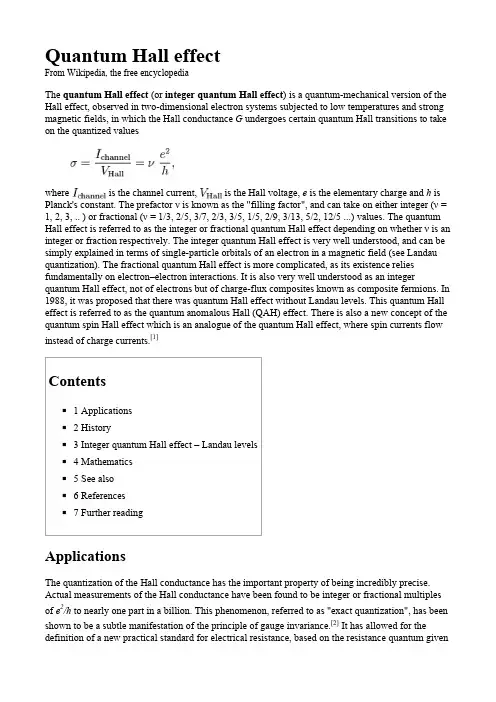
Quantum Hall effectFrom Wikipedia, the free encyclopediaThe quantum Hall effect (or integer quantum Hall effect) is a quantum-mechanical version of the Hall effect, observed in two-dimensional electron systems subjected to low temperatures and strong magnetic fields, in which the Hall conductance G undergoes certain quantum Hall transitions to take on the quantized valueswhere is the channel current, is the Hall voltage, e is the elementary charge and h is Planck's constant. The prefactor ν is known as the "filling factor", and can take on either integer (ν = 1, 2, 3, .. ) or fractional (ν = 1/3, 2/5, 3/7, 2/3, 3/5, 1/5, 2/9, 3/13, 5/2, 12/5 ...) values. The quantum Hall effect is referred to as the integer or fractional quantum Hall effect depending on whether ν is an integer or fraction respectively. The integer quantum Hall effect is very well understood, and can be simply explained in terms of single-particle orbitals of an electron in a magnetic field (see Landau quantization). The fractional quantum Hall effect is more complicated, as its existence relies fundamentally on electron–electron interactions. It is also very well understood as an integer quantum Hall effect, not of electrons but of charge-flux composites known as composite fermions. In 1988, it was proposed that there was quantum Hall effect without Landau levels. This quantum Hall effect is referred to as the quantum anomalous Hall (QAH) effect. There is also a new concept of the quantum spin Hall effect which is an analogue of the quantum Hall effect, where spin currents flow instead of charge currents.[1]Contents◾1 Applications◾2 History◾3 Integer quantum Hall effect – Landau levels◾4 Mathematics◾5 See also◾6 References◾7 Further readingApplicationsThe quantization of the Hall conductance has the important property of being incredibly precise. Actual measurements of the Hall conductance have been found to be integer or fractional multiples of e2/h to nearly one part in a billion. This phenomenon, referred to as "exact quantization", has been shown to be a subtle manifestation of the principle of gauge invariance.[2] It has allowed for the definition of a new practical standard for electrical resistance, based on the resistance quantum givenby the von Klitzing constant R K = h/e2 = 25812.807557(18) Ω.[3] This is named after Klaus von Klitzing, the discoverer of exact quantization. Since 1990, a fixed conventional value R K-90 is used in resistance calibrations worldwide.[4] The quantum Hall effect also provides an extremely precise independent determination of the fine structure constant, a quantity of fundamental importance in quantum electrodynamics.HistoryThe integer quantization of the Hall conductance was originally predicted by Ando, Matsumoto, and Uemura in 1975, on the basis of an approximate calculation which they themselves did not believe to be true. Several workers subsequently observed the effect in experiments carried out on the inversion layer of MOSFETs. It was only in 1980 that Klaus von Klitzing, working at the high magnetic field laboratory in Grenoble with silicon-based samples developed by Michael Pepper and Gerhard Dorda, made the unexpected discovery that the Hall conductivity was exactly quantized. For this finding, von Klitzing was awarded the 1985 Nobel Prize in Physics. The link between exact quantization and gauge invariance was subsequently found by Robert Laughlin. Most integer quantum Hall experiments are now performed on gallium arsenide heterostructures, although many other semiconductor materials can be used. In 2007, the integer quantum Hall effect was reported in graphene at temperatures as high as room temperature,[5] and in the oxide ZnO-Mg x Zn1-x O.[6] Integer quantum Hall effect – Landau levelsIn two dimensions, when classical electrons are subjected to a magnetic field they follow circular cyclotron orbits. When the system is treated quantum mechanically, these orbits are quantized. The energy levels of these quantized orbitals take on discrete values: , where ωc = eB/m is the cyclotron frequency. These orbitals are known as Landau levels, and at weak magnetic fields, their existence gives rise to many interesting "quantum oscillations" such as the Shubnikov–de Haas oscillations and the de Haas–van Alphen effect (which is often used to map the Fermi surface of metals). For strong magnetic fields, each Landau level is highly degenerate (i.e. there are many single particle states which have the same energy E n). Specifically, for a sample of area A, inmagnetic field B, the degeneracy of each Landau level is (where g s represents a factor of 2 for spin degeneracy, and is the magnetic flux quantum). ForHofstadter's butterfly sufficiently strong B-fields, each Landau level may have so many states that all of the free electrons in the system sit in only a few Landau levels; it is in this regime where one observes the quantum Hall effect.MathematicsThe integers that appear in the Hall effect are examples oftopological quantum numbers. They are known inmathematics as the first Chern numbers and are closelyrelated to Berry's phase. A striking model of much interest inthis context is the Azbel-Harper-Hofstadter model whosequantum phase diagram is the Hofstadter butterfly shown inthe figure. The vertical axis is the strength of the magneticfield and the horizontal axis is the chemical potential, whichfixes the electron density. The colors represent the integer Hall conductances. Warm colors represent positive integersand cold colors negative integers. The phase diagram isfractal and has structure on all scales. In the figure there is an obvious self-similarity.Concerning physical mechanisms, impurities and/or particular states (e.g., edge currents) are important for both the 'integer' and 'fractional' effects. In addition, Coulomb interaction is also essential in the fractional quantum Hall effect. The observed strong similarity between integer and fractional quantum Hall effects is explained by the tendency of electrons to form bound states with an even number of magnetic flux quanta, called composite fermions .See also◾quantum Hall transitions◾Fractional quantum Hall effect◾Composite fermions◾Hall effect◾Hall probe◾Graphene◾Quantum spin Hall effect◾Coulomb potential between two current loops embedded in a magnetic fieldReferences1.^ Ezawa, Zyun F. (2013). Quantum Hall Effects: Recent Theoretical and Experimental Developments (3rd ed.). World Scientific. ISBN 978-981-4360-75-3.2.^ Laughlin, R. (1981). "Quantized Hall conductivity in twodimensions" (/abstract/PRB/v23/i10/p5632_1). Physical Review B 23 (10): 5632–5633. Bibcode:1981PhRvB..23.5632L (/abs/1981PhRvB..23.5632L).doi:10.1103/PhysRevB.23.5632 (/10.1103%2FPhysRevB.23.5632). Retrieved 8 May 2012.3.^ Tzalenchuk, Alexander; Lara-Avila, Samuel; Kalaboukhov, Alexei; Paolillo, Sara; Syväjärvi, Mikael;Yakimova, Rositza; Kazakova, Olga; Janssen, T. J. B. M.; Fal'ko, Vladimir; Kubatkin, Sergey (2010)."Towards a quantum resistance standard based on epitaxialgraphene" (/nnano/journal/v5/n3/abs/nnano.2009.474.html). NatureNanotechnology5 (3): 186–189. arXiv:0909.1220 (https:///abs/0909.1220).Bibcode:2010NatNa...5..186T (/abs/2010NatNa...5..186T).doi:10.1038/nnano.2009.474 (/10.1038%2Fnnano.2009.474). PMID 20081845(https:///pubmed/20081845).4.^ "conventional value of von Klitzing constant" (/cgi-bin/cuu/Value?rk90). NIST.5.^ Novoselov, K. S.; Jiang, Z.; Zhang, Y.; Morozov, S. V.; Stormer, H. L.; Zeitler, U.; Maan, J. C.;Boebinger, G. S.; Kim, P.; Geim, A. K. (2007). "Room-Temperature Quantum Hall Effect in Graphene".Science315 (5817): 1379. arXiv:cond-mat/0702408 (https:///abs/cond-mat/0702408).Bibcode:2007Sci...315.1379N (/abs/2007Sci...315.1379N).doi:10.1126/science.1137201 (/10.1126%2Fscience.1137201). PMID 17303717(https:///pubmed/17303717).6.^ Tsukazaki, A.; Ohtomo, A.; Kita, T.; Ohno, Y.; Ohno, H.; Kawasaki, M. (2007). "Quantum Hall Effectin Polar Oxide Heterostructures". Science315 (5817): 1388–91. Bibcode:2007Sci...315.1388T(/abs/2007Sci...315.1388T). doi:10.1126/science.1137430(/10.1126%2Fscience.1137430). PMID 17255474(https:///pubmed/17255474).Further reading◾Ando, Tsuneya; Matsumoto, Yukio; Uemura, Yasutada (1975). "Theory of Hall Effect in a Two-Dimensional Electron System". J. Phys. Soc. Jpn.39 (2): 279–288.Bibcode:1975JPSJ...39..279A (/abs/1975JPSJ...39..279A).doi:10.1143/JPSJ.39.279 (/10.1143%2FJPSJ.39.279).◾Klitzing, K.; Dorda, G.; Pepper, M. (1980). "New Method for High-Accuracy Determination of the Fine-Structure Constant Based on Quantized Hall Resistance". Phys. Rev. Lett.45 (6): 494–497. Bibcode:1980PhRvL..45..494K(/abs/1980PhRvL..45..494K). doi:10.1103/PhysRevLett.45.494(/10.1103%2FPhysRevLett.45.494).◾Laughlin, R. B. (1981). "Quantized Hall conductivity in two dimensions". Phys. Rev. B.23(10): 5632–5633. Bibcode:1981PhRvB..23.5632L(/abs/1981PhRvB..23.5632L). doi:10.1103/PhysRevB.23.5632(/10.1103%2FPhysRevB.23.5632).◾Yennie, D. R. (1987). "Integral quantum Hall effect for nonspecialists". Rev. Mod. Phys.59(3): 781–824. Bibcode:1987RvMP...59..781Y(/abs/1987RvMP...59..781Y). doi:10.1103/RevModPhys.59.781(/10.1103%2FRevModPhys.59.781).◾Hsieh, D.; Qian, D.; Wray, L.; Xia, Y.; Hor, Y. S.; Cava, R. J.; Hasan, M. Z. (2008). "A topological Dirac insulator in a quantum spin Hall phase". Nature452 (7190): 970–974.arXiv:0902.1356 (https:///abs/0902.1356). Bibcode:2008Natur.452..970H(/abs/2008Natur.452..970H). doi:10.1038/nature06843(/10.1038%2Fnature06843). PMID 18432240(https:///pubmed/18432240).◾25 years of Quantum Hall Effect, K. von Klitzing, Poincaré Seminar (Paris-2004). Postscript (http://parthe.lpthe.jussieu.fr/poincare/textes/novembre2004.html). Pdf(/PhysicsHorizon/25yearsQHE-lecture.pdf).◾Magnet Lab Press Release Quantum Hall Effect Observed at Room Temperature (/mediacenter/news/pressreleases/2007february15.html)◾Avron, Joseph E.; Osadchy, Daniel, Seiler, Ruedi (2003). "A Topological Look at the Quantum Hall Effect" (/resource/1/phtoad/v56/i8/p38_s1).Physics Today56 (8): 38. Bibcode:2003PhT....56h..38A(/abs/2003PhT....56h..38A). doi:10.1063/1.1611351(/10.1063%2F1.1611351). Retrieved 8 May 2012.◾Zyun F. Ezawa: Quantum Hall Effects - Field Theoretical Approach and Related Topics.World Scientific, Singapore 2008, ISBN 978-981-270-032-2◾Sankar D. Sarma, Aron Pinczuk: Perspectives in Quantum Hall Effects. Wiley-VCH, Weinheim 2004, ISBN 978-0-471-11216-7◾Baumgartner, A.; Ihn, T.; Ensslin, K.; Maranowski, K.; Gossard, A. (2007). "Quantum Hall effect transition in scanning gate experiments". Physical Review B76 (8).Bibcode:2007PhRvB..76h5316B (/abs/2007PhRvB..76h5316B).doi:10.1103/PhysRevB.76.085316 (/10.1103%2FPhysRevB.76.085316).◾E. I. Rashba and V. B. Timofeev, Quantum Hall Effect, Sov. Phys. - Semiconductors v. 20, pp.617-647 (1986).Retrieved from "/w/index.php?title=Quantum_Hall_effect&oldid=605304404"Categories: Hall effect Condensed matter physics Quantum electronics SpintronicsQuantum phases Mesoscopic physics◾This page was last modified on 22 April 2014 at 14:51.◾Text is available under the Creative Commons Attribution-ShareAlike License; additional terms may apply. By using this site, you agree to the Terms of Use and Privacy Policy.Wikipedia® is a registered trademark of the Wikimedia Foundation, Inc., a non-profitorganization.。

Scientia Iranica B(2011)18(4),923–929Sharif University of TechnologyScientia IranicaTransactions B:Mechanical EngineeringExperimental investigation of air–water,two-phase flow regimes in vertical mini pipeP.Hanafizadeh,M.H.Saidi∗,A.Nouri Gheimasi,S.GhanbarzadehSchool of Mechanical Engineering,Sharif University of Technology,Tehran,P.O.Box11155-9567,IranReceived8November2010;revised28April2011;accepted12June2011KEYWORDSMini pipes;Two-phase flow; Flow pattern; Visualization; Flow pattern map.Abstract In this study,the flow patterns of air–water,two-phase flows have been investigated experimentally in a vertical mini pipe.The flow regimes were observed by a high speed video recorder in pipes with diameters of2,3and4mm and length27,31and25cm,respectively.The comprehensive visualization of air–water,two-phase flow in a vertical mini pipe has been performed to realize the physics of such a two-phase flow.Different flow patterns of air–water flow were observed simultaneously in the mini pipe at different values of air and water flow rates.Consequently,the flow pattern map was proposed for flow in the mini-pipe,in terms of superficial velocities of liquid and gas phases.The flow pattern maps are compared with those of other researchers in the existing literature,showing reasonable agreement.©2011Sharif University of Technology.Production and hosting by Elsevier B.V.All rights reserved.1.IntroductionGas–liquid,two-phase flow in micro structures has played an important role in several industrial and medical applications, such as micro heat exchangers,lab-on-chips,bio-MEMS and micro cooling electronics.Physical perception of micro flows is critical in order to optimize and develop the design of such devices.Two-phase flows at mini and micro scale have recently attracted the attention of scientists as a result of its wide usage in advanced science and technology,namely Micro-Electro-Mechanical Systems(MEMS),chemical engineering, bioengineering,medical devises,micro cooling systems,micro structures in computers,etc.The literature survey on this issue has been categorized into adiabatic and phase change work, which has been summarized in this paper.∗Corresponding author.E-mail address:saman@(M.H.Saidi).1.1.Adiabatic worksThe works of Suo and Griffith[1]were among the first studies concentrating on flow patterns in microchannels.They detected three different flow patterns,namely,bubbly/slug, slug and annular flow,in their studies,using channels with widths in the range of0.514–0.795mm.Sadatomi et al.[2] proposed flow regime maps in vertical rectangular channels and indicated that channel geometries have little influence in noncircular channels with large hydraulic diameters greater than10mm.Xu et al.[3]investigated concurrent vertical two-phase flow in a vertical rectangular channel with a narrow gap, experimentally.They reported that with a decrease in channel gap,the transition from one flow regime to another occurs at smaller gas flow rates.They developed a new criterion to predict transition from annular flow,as well.Hestroni et al.[4] performed experiments for air–water and steam–water flow in parallel triangular micro-channels,developed a practical modeling approach for two-phase micro-channel heat sinks and considered the discrepancy between flow patterns of air–water and steam–water flow in parallel micro-channels. Fukagata et al.[5]simulated an air–water two-phase flow in a20µm ID tube,numerically,with focus upon flow and heat transfer characteristics in the bubble train flows.He and Kasagi[6]simulated numerically adiabatic air water slug flow in a micro tube.They focused on pressure drop characteristics and their modeling.They found that the total pressure drop of a slug flow can be decomposed into a frictional pressure drop and a pressure drop over the bubble itself.Carlson et al.[7]1026-3098©2011Sharif University of Technology.Production and hosting by Elsevier B.V.All rights reserved.Peer review under responsibility of Sharif University of Technology.doi:10.1016/j.scient.2011.07.003924P.Hanafizadeh et al./Scientia Iranica,Transactions B:Mechanical Engineering18(2011)923–929investigated characteristics of multiphase dynamics,especially two-phase gas–liquid flow,by means of advanced numerical simulations.They compared two Computational Multi-Fluid Dynamic(CMFD)codes,Fluent and TransAT,and reported a prediction of recirculating flow in the bubbly flow case using TransAT,while significant recirculation was not observed in the solution using Fluent.Saison and Wongwises[8]performed a series of experiments in a horizontal circular micro channel with an inner diameter of0.15mm.They presented a flow pattern map in terms of the phase superficial velocities, and proposed a new pressure drop correlation for practical application.1.2.Phase change worksThe pool boiling heat transfer,in a vertical narrow annular with closed bottoms,was observed through a transparent quartz shroud by Yao and Chang[9],and stages of evolving boiling phenomena with an increase in heat flux were reported. Several researchers observed three basic flow patterns,namely, bubbly,slug and annular flow,in the mini pipe and channel. Damianides and Westwater[10]performed experiments with a1mm tube,and Mertz et al.[11]and Kasza et al.[12] studied the flow visualization of water nucleation in a single rectangular channel of2.5mm by6mm.Lin et al.[13]used a single round tube with2.1mm inside diameter for their experiments,and compared the flow transitions with those predicted by Bernea et al.[14].Sheng and Palm[15]performed their experiments with1–4mm diameter tubes.Cornwell and Kew[16]found three different flow patterns for R-113, namely,isolated bubbles confined bubbles and slug/annular flow,in rectangular channels with cross sectional areas of 1.2–0.9mm and3.5–1.1mm.Ory et al.[17]considered the effects of capillary,inertia,friction and gravity forces on the velocity distribution and temperature field along a single capillary two-phase flow in a heated micro-channel.Research dealing with gas–liquid,two-phase flow in micro-channels,in situations where fluid inertia was significant in comparison with surface tension,was reviewed by Ghiaasiaan and Abdel-Khalik[18].Jiang et al.[19]studied the boiling of water in triangular micro-channels,having widths of50and100µm. They observed individual bubbles at low heat fluxes,and an abrupt change in flow pattern to an unstable slug flow with increasing heat flux.Chedester and Ghiaasiaan[20]addressed the hydro-dynamically controlled Onset of a Significant Void (OSV)in heated micro tubes.They derived a simple semi-empirical correlation for the radius of departing bubbles at the OSV point to show the accuracy of their hypothesis.Some experimental studies have been reported on gas liquid two-phase flow in mini and micro conduits by Kandlikar[21],Lee and Mudawar[22]and Serizawa et al.[23].The three zone boiling heat transfer model was developed by Thome et al.[24]. Revellin and Thome[25]used an optical measurement method for two-phase characteristics of R-134a and R-245fa,in0.5mm and0.8mm diameter channels,to determine the frequency of bubbles existing in the microevaporator.They detected four flow patterns,namely,bubbly,slug,semi-annular and annular flow,whose transitions were not well compatible with neither the macroscale map of refrigerants nor the microscale map of air–water flow.Sobierska et al.[26] experimentally investigated the water boiling phenomena in a vertical rectangular microchannel,with a hydraulic diameter of0.48mm.They observed three main flow patterns,namely, bubbly,slug and annularflow.Figure1:Schematic of test apparatus.Due to the effects of surface tension,two-phase flows at mini and micro scale have different behavior in comparison with the macro scale.The aim of the present work is to visualize flow regimes in air–water two-phase flows and propose a flow regime map for such flows in vertical mini pipes.The neural network technique is implemented to recognize and predict a gas–liquid,two-phase flow pattern in mini tubes,having diameters of2,3and4mm.2.Experimental setupThis study is carried out by experimental apparatus schematically shown in Figure1.Air and water are used as gas and liquid phases in the experiments.The water flow rates are regulated by the needle valves and are measured by the cali-brated rotameter.Air and water are mixed together in a mixer made of acrylic glass and placed at the bottom of the riser pipe. The compressed air is fed by the compressor via an air injec-tor,which is schematically depicted in Figure2.The water flows from the center hole of a mixer,with a diameter of2mm,while air is injected into the holes around the center hole,each having 1mm diameter.The air flow rates are set by the regulator valve and are continuously measured by the calibrated gas rotameter. The overall height and inside diameter of the riser pipe are sum-marized in Table1.In order to have the opportunity to visually observe the two-phase flow patterns,the riser pipe was made of transparent glass.The air water mixture was directed upward through the riser,separated in the separation tank at the top of the riser and the air was discharged into the atmosphere.Differ-ent flow regime images were captured by a digital high speed camera,with a frame rate of1200fps,from the test section of the upriser.The test section is placed after the entrance section to diminish the effect of the entrance region.The length of the entrance section is about500mm.The superficial air and water velocities are0.5–10m/s and0.05–1m/s,respectively.P.Hanafizadeh et al./Scientia Iranica,Transactions B:Mechanical Engineering 18(2011)923–929925Figure 2:Schematic of air and watermixer.Figure 3:(a)RGB picture;(b)gray picture;and (c)subtracting and median process of flow in the pipe (3mm diameter).3.Experimental results 3.1.Image processingImage processing techniques must be performed in order to extract features from the images of the two-phase flow.Each picture has 8bit RGB (red,green and blue)color format,being converted from RGB to a grey scale mode.The output image has 256grey levels from 0(black)to 255(white).It is difficult to extract the bubbles directly from an original digital image and therefore preprocessing procedures must be undertaken to reduce noise and improve the quality of the images.An image-subtracted algorithm was used to reduce background noise by subtracting the background image from each dynamic image.In order to smooth the image border,a median filter was also used.A sliding window (3×3)was used in this process,and the median gray level of the pixels in the window was ter,the gray level of the pixels located at the center of the window was replaced by the median.The result of these processes is shown in Figure 3.3.1.1.Inverting binary imageThe images were converted from grayscale to binary mode by threshold segmentation,and an iterative procedure was used to calculate the optimizing threshold as follows [27]:Figure 4:Binary image of two-phase flow in the mini pipe.(a)The minimum and maximum of the gray level,namely Z land Z k ,are found in the image,and the initial value of the threshold is derived from their arithmetic average as:T 0=(Z k +Z l )/2.(1)(b)According to the initial value of threshold T K ,the imageis divided into two parts,namely,object and background,and the average value of the gray level in each part is calculated as:Z O =−Z (i ,j )<T kZ (i ,j )N O,(2)Z B =−Z (i ,j )>T kZ (i ,j )N B,(3)where Z (i ,j )is the gray level of the pixel (i ,j )in the image,N O is the number of the pixels in which Z (i ,j )is less than T K ,and N B is the number of pixels in which Z (i ,j )is more than T K .(c)The new threshold is calculated based on the arithmeticaverage of the object and background segments of the image as:T k +1=(Z O +Z B )/2.(4)If T K =T K +1,then the algorithm is finished,else K ≪=K +1,and turn to step (b).The binary image of the bubbles in the vertical pipe,which is the result of the above procedure,is shown in Figure 4.3.1.2.Image morphology processingSome morphological functions,such as dilation,erosion,opening and closing operations,were applied to modify the shapes of bubbles.Dilation adds pixels to the boundaries of the objects in an image,while erosion removes pixels on the object boundaries.The definition of a morphological opening of an image is erosion followed by dilation,using the same structuring element for both operations.The related operation,morphological closing of an image,is the reverse.It consists of dilation followed by erosion,with the same structuring element.Both of them do not significantly alter the area or shape of objects.The opening operation removes small objects and smoothes boundaries.Borders removed by erosion are restored by dilation,but small objects that were absorbed during erosion do not reappear after dilation.The closing operation was used to fill tiny holes and smooth boundaries.Objects were expanded by dilation and then reduced by erosion,so borders were smoothed and holes were filled [28,29].After926P.Hanafizadeh et al./Scientia Iranica,Transactions B:Mechanical Engineering 18(2011)923–929Figure 5:Final image of two-phase flow in the mini pipe.these operations,the result of image processing is shown in Figure 5.Bubble images of two-phase flow were clear using the above image processing,and it prepared bubbles for quantitative analysis,such as measuring area,perimeter and diameter.3.2.Flow pattern mapIn the experimental procedure while varying gas or liquid mass flow rate,a 10s film was recorded from the flow regime at a speed of 1200fps.The recorded film was replayed in slow motion for recognition of flow regimes.Each film converted to separate frames in a picture format using Adobe Premiere software.The achieved pictures were used as inputs of image processing techniques.The final binary pictures were used for the mentioned post processing procedure,such as flow regimedetection,void fraction and bubble velocity calculation,etc.Figure 6shows those typical flow regimes observed in the vertical,co-current,air–water,two-phase flows,in the 3mm mini pipe.Four basic flow patterns,namely,bubbly,slug,churn and annular,accompanied by their transitions,are illustrated in these figures.The visualization shows that air–water two-phase flows in mini pipes do not have three dimensional behaviors,especially in bubbly and slug flows.The final processed images of different flow regimes in air–water,two-phase flow in mini pipes have been presented in Figure 7.Figures 8–10show the flow pattern map for a vertical round tube with inner diameters of 2,3and 4mm,respectively.The proposed maps are in terms of superficial velocities of phases,and the four main flow patterns are depicted in these maps.In Figure 11,the achieved flow pattern for the pipe with 2mm ID was compared to the work of Ide et al.[30],shown by a solid line.They divided the flow pattern map into the four main regions,namely,dispersed bubbly flow,intermittent flow,churn flow and annular flow.The comparison shows that the bubbly and annular flows in the present work are not well in accordance with those of Ide et al.In the present work,the dispersed bubbles were not seen,because the air bubble injector did not have very thin holes.As a result,the created bubbles mostly have diameters in the range of the pipe diameter.Even the existence of air injectors with thin holes cannot guarantee the creation of bubbly flow.In the case of small bubbles occurring,as a result of thin holes in the air injector and the developed two-phase flow,they would collapse,resulting in large bubbles know as intermittent flow.Bubbly flows are mainly promoted by bubble breaking mechanisms,due to turbulence effects.It seems that in small diameter pipes,the formation of a specific flowpatterns(a)Bubbly.(b)Bubbly-slug.(c)Slug.(d)Messy-slug.(e)Churn.(f)Wispy-annular.(g)Ring.(h)Wavy-annular.(i)Annular.Figure 6:Different flow patterns in a vertical pipe with 2mm diameter.P.Hanafizadeh et al./Scientia Iranica,Transactions B:Mechanical Engineering18(2011)923–929927(a)Bubbly.(b)Slug.(c)Messy-slug.(d)Churn.(e)Ring.(f)Wavy-annular.Figure7:Final processed image of different two-phase flow regimes in the minipipe.Figure8:Flow patterns for2mm innerdiameter.Figure9:Flow patterns for3mm inner diameter.mainly depends on mixer configuration.The radial air supplierused in this study makes intermittent flow patterns,such asslug and churn flows,while the air supply in the tube centerfavors annular flow.This can be the reason for an absence ofannular flow in the proposed flow patterns.The comparison offlow patterns also reveals that the slug,messy slug andsemi-Figure10:Flow patterns for4mm inner diameter.annular flows in the proposed map are in accordance with theintermittent flow of Ide et al.[30].In the present study,a noticeable difference between flowpattern maps for vertical pipes with various diameters of2,3and4mm is not seen.This can be justified in regard tothe fact that the dominant forces acting on the air–watermixture in the small diameter pipes,namely,gravitation,inertia,surface tension and buoyancy forces,are in the sameorder of magnitude.This concept clearly indicates that thesethree flow patterns can be combined to form a new flow patternfor the gas–liquid,two-phase flow in small diameter pipes.A combination of these three flow patterns results in a newflow pattern map,which is illustrated in Figure12.A FuzzyC-Means clustering technique(FCM)was used to classify theflow patterns.The solid lines in the figure show the transitionregion of the flow patterns.This figure shows the achieved flowmap for mini pipes with diameters in the range of2–4mm.4.ConclusionIn this paper,air–water,two-phase flow patterns wereinvestigated experimentally for mini pipes with diameters of2,3and4mm.An image processing technique was used fordetection of flow patterns from pictures derived from filmsrecorded with a high speed camcorder.The obtained flowpatterns reveal that there is no noticeable difference between928P.Hanafizadeh et al./Scientia Iranica,Transactions B:Mechanical Engineering 18(2011)923–929Figure 11:Comparison between the achieved flow patterns with the work of Ide et al.[30]for a pipe with diameter of 2mm.Figure 12:Proposed two-phase vertical upward flow pattern map.two-phase,upward flow patterns in this range of diameters.A new flow pattern map was achieved for vertical mini pipes,due to a comparison of the flow patterns of these three diameters of pipe.The proposed map was compared with existing research.A comparison of the present work and previous research shows that the flow patterns of slug,messy slug and semi-annular in the present work are compatible with the intermittent flow pattern of Ide et al.[30].However,in the present study,the annular flow is seen at a lower superficial air velocity than that in the work of Ide et al.[30].AcknowledgmentsThis research was funded by Iran Supplying Petrochemical Industries,Parts,Equipment and Chemical Design Corporation (SPEC),as a joint research project with Sharif University of Technology (project No.KPR-8628077).References[1]Suo,M.and Griffith,P.‘‘Two-phase flow in capillary tubes’’,Int.J.Basic Eng.,86,pp.576–582(1964).[2]Sadatomi,Y.,Sato,Y.and Saruwatari,S.‘‘Two-phase flow in verticalnoncircular channels’’,Int.J.Multiphase Flow ,8,pp.641–655(1982).[3]Xu,J.L.,Cheng,P.and Zhao,T.S.‘‘Gas–liquid two-phase flow regimes inrectangular channels with mini/micro gaps’’,Int.J.Multiphase Flow ,25,pp.411–432(1999).[4]Hetsroni,G.,Mosyak, A.,Segal,Z.and Pogrebnyak, E.‘‘Two-phaseflow patterns in parallel micro-channels’’,Int.J.Multiphase Flow ,29,pp.341–360(2003).[5]Fugakata,K.,Kasagi,N.,Ua-arayaporn,P.and Himeno,T.‘‘Numericalsimulation of gas liquid two-phase flow and convective heat transfer in a micro tube’’,Int.J.Heat and Fluid Flow ,28,pp.72–82(2007).[6]He,Q.and Kasagi,N.‘‘Numerical investigation on flow pattern andpressure drop characteristics of slug flow in a micro tube’’,6th Int.ASME Conf.on Nanochannels,Microchannels and Minichannels ,Darmstadt,Germany,pp.24–35(2008).[7]Carlson,A.,Kudinov,P.and Narayanan,C.‘‘Prediction of two-phase flowin small tubes:a systematic comparison of state-of-the-art CMFD codes’’,5th Europe Thermal-Sci.Conf.,The Netherlands,pp.138–150(2008).[8]Saisorn,S.and Wongwises,S.‘‘An experimental investigation of two-phaseair–water flow through a horizontal circular micro-channel’’,Exp.Thermal Fluid Sci.,33,pp.306–315(2009).[9]Yao,S.C.and Chang,Y.‘‘Pool boiling heat transfer in a confined space’’,Int.J.Heat Mass Transf.,26,pp.841–848(1983).[10]Damianides,D.A.and Westwater,J.W.‘‘Two-phase flow patterns in acompact heat exchanger and in small tubes’’,2nd UK National Conf.on Heat Transf.,11,United Kingdom,London,pp.1257–1268(1988).[11]Mertz,R.,Wein,A.and Groll,C.‘‘Experimental investigation of flow boilingheat transfer in narrow channels’’,Calore e Technologia ,14(2),pp.47–54(1996).[12]Kasza,K.E.,Didascalou,T.and Wambsganss,M.W.‘‘Microscale flow visu-alization of nucleate boiling in small channels:mechanisms influencing heat transfer’’,Int.Conf.on Compact Heat Exchanges for the Process Indus-tries ,New York,USA,pp.343–352(1997).[13]Lin,S.,Kew,P.A.and Cornwell,K.‘‘Two-phase flow regimes and heattransfer in small tubes and channels’’,11th Int.Heat Transf.Conf.,Kyongju,Korea,2,pp.45–50(1998).[14]Barnea,D.,Luninsky,Y.and Taitel,Y.‘‘Flow pattern in horizontal andvertical two-phase flow in small diameter pipes’’,Canadian J.Chem.Eng.,61,pp.617–620(1983).[15]Sheng, C.H.and Palm, B.‘‘The visualization of boiling in small-diameter tubes’’,Int.Conf.on Heat Transport and Transport Phenomena in Microsystems ,Banff,Canada,pp.44–53(2001).[16]Cornwell,K.and Kew,P.A.‘‘Boiling in small parallel channels’’,CEC Conf.on Energy Eff.in Process Tech.,Athens,Greece,pp.624–638(1992).[17]Ory, E.,Yuan,H.,Prosperetti, A.,Popinet,S.and Zaleski,S.‘‘Growthand collapse of a vapor bubble in a narrow tube’’,Phys.Fluids ,12,pp.1268–1277(2000).[18]Ghiaasiaan,S.M.and Abdel-Khalik,S.I.‘‘Two-phase flow in micro-channels’’,Adv.Heat Transf.,34,pp.145–253(2001).[19]Jiang,L.,Wong,M.and Zohar,Y.‘‘Forced convection boiling in a micro-channel heat sink’’,Int.J.Micro-Electro-Mech.Sys.,10,pp.80–87(2000).[20]Chedester,R.C.and Ghiaasiaan,S.M.‘‘A proposed mechanism for hydrodynamically-controlled onset of significant void in microtubes’’,Int.J.Heat Fluid Flow ,23,pp.769–775(2002).[21]Kandlikar,S.G.‘‘Fundamental issues related to flow boiling in minichan-nels and microchannels’’,Exp.Therm.Fluid Sci.,26,pp.389–407(2002).[22]Lee,J.and Mudawar,I.‘‘Two phase flow in high heat flux micro channelheat sink for refrigeration cooling applications’’,Int.J.Heat Mass Transf.,48,pp.928–955(2005).[23]Serizawa,A.‘‘Gas liquid two-phase flow in microchannels’’,In MultiphaseFlow Handbook ,C.T.Crowe,Ed.,2nd ed.,pp.830–887,CRC Press (2006).[24]Thome,J.R.,Dupont,V.and Jacobi, A.M.‘‘Heat transfer model forevaporation in micro channels’’,Int.J.Heat Mass Transf.,47,pp.3375–3385(2004).P.Hanafizadeh et al./Scientia Iranica,Transactions B:Mechanical Engineering18(2011)923–929929[25]Revellin,R.and Thome,J.R.‘‘Experimental investigation of R-134a andR-245fa two-phase flow in microchannels for different flow conditions’’, Int.J.Heat Fluid Flow,28,pp.63–71(2007).[26]Sobierska, E.,Kulenovic,R.and Mertz,R.‘‘Heat transfer mechanismand flow pattern during flow boiling of water in a vertical narrow channel experimental results’’,Int.J.Thermal Sci.,46,pp.1172–1181 (2007).[27]Shi,L.‘‘Fuzzy recognition for gas–liquid two-phase flow pattern based onimage processing’’,Proc.of13rd IEEE Int.Conf.on Control and Automation, pp.1424–1427(2007).[28]Heijmans,H.J.A.M.,Morphological Image Operators,Academic Press,NewYork(1994).[29]/help/toolbox/images/index.html.[30]Ide,H.,Kariyasaki,A.and Fukano,T.‘‘Fundamental data on the gas–liquidtwo-phase flow in minichannels’’,Int.J.Thermal Sci.,46,pp.519–530 (2007).Pedram Hanafizadeh received his M.S.and Ph.D.Degrees in Mechanical Engineering from the Centre of Excellence in Energy Conversion at Sharif University of Technology,Tehran,Iran,in2005and2010,respectively.His work is mainly concentrated on the field of Multiphase Flow,Experimentally, Numerically and Analytically.His research interests include Characteristics of Multiphase Flow,Heat Transfer,Boiling and Condensation,Instrumentation in Fluid Flow,Image Processing for Flow Field Analysis,and Industrial and Applicable Usage of Multiphase Flow.Mohammad Hassan Saidi is Professor and Chairman of the School of Mechanical Engineering at Sharif University of Technology,Tehran,Iran. His current research interests include Multiphase Flows,Heat Transfer Enhancement in Boiling and Condensation,Modelling of Pulse Refrigeration, Vortex Tube Refrigerator,Indoor Air Quality and Clean Room Technology, Energy Efficiency in Home Appliances and Desiccant Cooling Systems.Arash Nouri Gheimasi obtained his B.S.Degree in Mechanical Engineering in2010,and is currently an M.S.student at the Centre of Excellence in Energy Conversion at the School of Mechanical Engineering,Sharif University of Technology,Tehran,Iran,under the supervision of Professor Saidi.His B.S. thesis involved work on the Characteristics of Gas-Liquid Two-Phase Flow in Mini Pipes and he is now working on Application of Visual Techniques in Two-Phase Flow.His research interests include the area of Two Phase Flow and Its Industrial Applications.Soheil Ghanbarzade received his B.S.and M.S.Degrees in Mechanical Engineering from the Centre of Excellence in Energy Conversion at Sharif University of Technology in2008and2010,respectively.Since then he has worked under the supervision of Professor M.H.Saidi as research staff in the Multiphase Group.His research interests include:Analytical,Numerical and Experimental Methods to Study Characteristics of Large Scale and Mini Scale Air-Water,Two-Phase Flows.He holds a Gold medal from the13th National Olympiad of Mechanical Engineering in Iran,and is currently a Ph.D.student of Petroleum Engineering at the University of Texas,Austin,USA.。

A note on quadratic convergence of smoothing Newton algorithm for the LCP BiFeO3/TiO2 Nanotube Arrays Composite Electrode: Construction,
朱阿姝 Characterization, and Enhanced Photoelectrochemical Properti 刘凤山 发现迄今最遥远的cD型星系 Holographic femions on a charged Lifshitz background from 吴健聘 Einstein-Dilaton-Maxwell model 吴亚波 物质与曲率耦合的广义f(R)引力的热力学性质 Role of intensity fluctuations in third-order correlation 陈希浩 double-slit interference of thermal light(热光源的强度涨落在三 阶双缝干涉中的作用) 李荣德 喷射成形7075合金回归再时效处理的组织和抗应力腐蚀性能 Research on rotary surface topography by orthogonal turn朱立达 milling正交车铣加工表面形貌的研究 Study of Crown Three-Dimension Model Rebuilding Based on RE 张德强 Technology and Its Laser RP Technology 杨秀英 Al颗粒尺寸对γ '/复合涂层结构及性能影响 耿佃桥 行波磁场对RH精炼过程流场、混合、脱碳及夹杂物去除的影响 袁野 不确定图数据的高效关键字查询 Vehicle Type Classification by Acoustic Waves with Dimension 齐晓轩 Reduction Technique 刘颖 一种基于改进广义趋势扩散法的数据填补技术

岩土工程专业词汇——A辑•absorbed water 吸着水•aging 老化abutment 桥台•allowable bearing capacity 容许承载力•acoustic emission of rock 岩石声发射•allowable settlement 容许沉降•acoustic prospecting 声学探测•alluvial fan 冲积扇•active earth pressure 主动土压力•alluvial soil 冲积土•alternating load 交变荷载•active fault 活断层•anchoring，bolting 锚固bolting（螺栓连接, 拧紧）•activity index 活动性指数•anchor slab wall 锚定板墙•additional stress,superimposed stress 附加应力•anticline 背斜•aquifer 含水层•adverse geologic phenomena 不良地质现象•artesian(自流井的) pressure head 承压水头•aeolian deposit 风积土•artificial fill 人工填土•aeration(通风) zone water 包气带水•attitude 产状•average thickness method 平均厚度法•aggregate for concrete 混凝土骨料岩土工程专业词汇——B辑•back analysis 反演分析•bearing capacity factor 承载力因数•base course 道路基层•bearing stratum 持力层•bed rock 基岩•berm 反压平台( 反压马道) •boulder(stone block) 漂石( 块石) •Biot consolidation theory 比奥固结理论•Boussinesq theory 布辛涅斯克理论•Bishop's somplified method of slices 毕肖普简化条分法•bridge pier 桥墩brittle failure 脆性破坏•bulk modulus 体积模量blasting 爆破•buoyancy 浮托力block theory 块体理论•buttress retaining wall 支墩式挡墙•body force 体积力borrow area 取土场•by-pass seepage 绕渗岩土工程专业词汇——C辑•Cahtornia Bearing Ratio(CBR) 加州承载比•cobble 卵石( 碎石) •coefficient of collapsibility 湿陷系数•cantilever retaining wall 悬臂式挡墙•coefficient of compressibility 压缩系数•capillary water 毛细管水•categortzatlon of geotechnical projects 岩土工程分级•coefficient of consolidation 固结系数•cemment stabilization 水泥加固•coefficient of curvature 曲率系数•central load 中心荷载( 轴心荷载) •coefficient of deformation due to leaching 溶滤变形系数•Cerruti‘ssolution 色卢铁解答•coefficient of permeability 渗透系数•check dam 谷坊chemical grouting 化学灌浆•coeffieient of secondary consolidation 次固结系数•coarse aggregate 粗骨料•coefficient of self-weight collapsibility 自重湿陷系数•coarse-grained soil 粗粒土•coefficient of uniformity 均匀系数•compression index 压缩指数•coefficient of viscosity 粘滞系数•compressive strength 抗压强度•coefficient of volume compressibility 体积压缩系数•concentrated load 集中荷载( 点荷载) •coefficient of weathering 风化系数•concrete faced rockfill dam 混凝土面板堆石坝•cohesion 粘聚力•cone penetration test(CPT) 静力触探试验•cohesionless soil 无粘性土•cohesive soil 粘性土•confined warer 承压水•collapsibility 湿陷性•consistency limit 稠度界限•collapsibility test of loess 黄土湿陷试验•consolidated-drained triaxial test 固结排水三轴试验•collapsible soil 湿陷性土•consolidated quick shear test 固结快剪试验•combined bolting and shotcrete 喷锚支护•consolidated - undrainbd triaxial test 固结不排水三轴试验•compaetibility 压实性•compaction by rolling 碾压法•compaction grouting method 挤密喷浆法•consolidation 固结•consolidation cure 固结曲线岩土工程专业词汇——C辑•compacting mechinery 碾压机械•consolidation grouting 固结灌浆•compaction test 击实试验•composite ground 复合地基•consolidation settlement 固结沉降•composite slip surface 复合滑动面•consolidation test 固结试验•comprehensive engineering geological map 综合工程地质图岩土工程专业词汇——C辑•constitutive relation of soil土的本构关系( 本构模型) •comoressibility 压缩性•constrained grain size 限制粒径•Coulomb's earth pressure theory库仑土压力理论•counterfort retaining wall 扶壁式挡墙•constrained modulus 压缩模量•crack growth 裂纹扩展creep 蠕变•contact pressure 基底压力( 接触压力) •critical edge pressure 临塑荷载•contour map of groundwater 地下水等水位线图•critical height of slope( 土坡) 临界高度•control of underground water 地下水控制•critical hydraulic gradient 临界水力梯度•core of rock 岩芯•core recovery 岩芯采取率•critical void ratio 临界孔隙比•core wall 心墙•corner-points method 角点法•cross - hole method 跨孔法•curtain grouting 帷幕灌浆•Coulomb - Navier strength theory 库仑—纳维强度理论•cushion 垫层cutting 路堑•cutoff wall 截水墙cyclic load 周期荷载岩土工程专业词汇——D辑•Darcy's law 达西定律•Degree of consolidation 固结度•debris flow 泥石流•degree of saturation 饱和度•deep mixing method 深层搅拌法•delayed elasticity 弹性后效•deep soil stabilization 深层土加固•densification by explosion 爆炸加密法•deep well method 深井法•degree of compaction 压实度•densification by sand pile 挤密砂桩•density 密度•depletion coefficient 疏干系数•dispersion coefficient 弥散系数•developing chart of exploratory drift坑洞展示图•dispersive clay 分散性粘土•disturbed soil sample 扰动土样•dewatering method 降水法•differential settlement 沉降差•diversion tunnel 导流洞•down-hole method 下孔法•dike ，levee 堤drainage method 排水法•dilatancy 剪胀性dynamic consolidation 强夯法•dilatancy of rock 岩石扩容•dynamic load 动荷载diluvial fan 洪积扇•dynamic penetration test 动力触探试验•diluvial soil 洪积土[ dai’lju:vjel ]•direct shear test 直剪试验•dynamic simple shear test 动单剪试验•disaster geology 灾害地质学•dynamic triaxial test 动三错轴试验•dislocation 位错岩土工程专业词汇——E辑•earth dam 土坝•effective grain size 有效粒径•earth material 土料•earth pressure at rest 静止土压力•effective porosity 有效孔隙率•effective stress 有效应力•earthquake engineering 地震工程学•effective stress analysis 有效应力分析•earthquake subsidence 震陷•elastic strain 弹性应变•electrical prospecting 电法勘探•earth — rock dam 土石坝•earthwork 土石方工程electro-osmosis 电渗法•eccentric load 偏心荷载embankment 路堤•engineering geologic columnar profile •工程地质柱状图•environmental geotechnics 环境岩士工程•engineering geologic exploration 工程地质勘探•equipotential line 等势线•engineering geologic drilling 工程地质钻探•equivalent opening size(EOS) 等效孔径•engmeering geologic evaluation 工程地质评价•excavating machinery 挖掘机械•engineering geologic map 工程地质图•excavation 挖方•excess pore water pressure 超静水压力•engineering geologic mapping 工程地质测绘•expanded polystyrene(EPS) [ ’poli ’staieri:n ]•聚苯乙烯发泡材料•engineering geologic profile 工程地质剖面图•expansive soil 膨胀土岩土工程专业词汇——F辑•fabric sheet reinforced earth 铺网法•fine-grained soil 细粒土fissuerd clay 裂隙粘土•factor of safety 安全系数fissure water 裂隙水•failure strength 破坏强度•flat jack technique 扁千斤顶法•fall of ground 冒顶fatigue strength 疲劳强度•flow line 流线fault 断层•flow net 流网•field identification of soil 土的现场鉴别•fold 褶皱fraction 粒组•field observation 现场观测•fracture mechanics 断裂力学•fill 填方fracture zone 断裂破碎带•filter 反滤层free face 临空面•final settlement 最终沉降•free swelling ratio 自由膨胀率•fine aggregate 细骨料free water 自由水•frost heave 冻胀freezing method 冻结法•frost — heave capacity 冻胀量•french drain 盲沟fresh rock 新鲜岩石•frost heaving pressure 冻胀力•friction — resistance ratio 摩阻比•frozen soil 冻土岩土工程专业词汇——G辑•gap — graded soil 不连续级配土•geosynthetics 土工合成材料•geotechnical centrifugal model土工离心模型试验•general shear failure 整体剪切破坏•geotechnical engineering 岩土工程•geocomposite 土工复合材料•geotechnical engineering investigation 岩土工程勘察•Geodrain/prefabricated（预制）strip drain 塑性排水带法•Geofabriform 土工模袋geogrid 土工格栅•geotextiles 土工织物•geologic environment 地质环境•gradation 级配grain size 粒径•grain size distribution curve 粒径分布曲线•geologic structure 地质构造•gravelly soil 砾类土gravitational water重力水•geomechanical model test 地质力学模型试验•gravity retaining wall 重力式挡墙•geomembrane 土工膜geomorphology 地貌•Griffith 's strength criterion 格里菲斯强度准则•geophysical exploration 地球物理勘探•ground fracturing 地裂ground water 地下水•ground treatment 地基处理•geostatic stress 自重应力岩土工程专业词汇——G辑•groundwater dynamics 地下水动力学•groundwater regime 地下水动态•groundwater storage 地下水贮藏量•groundwater hardness 地下水硬度•groundwater monitoring 地下水监测•groin，spur dike丁坝grouting 灌浆•groundwater pollution 地下水污染•grouting test 灌浆试验guide adit 导洞•groundwater recharge 地下水补给量岩土工程专业词汇——H辑•hardness degree of rock 岩石坚硬程度•hydrogeological drilling 水文地质钻探•hydrogeological investigation 水文地质勘查•hydraulic fracturing technique 水力劈裂法•hydrogeology 水文地质学•hydrostatic pressure 静水压力•hydraulic fill 水力冲填•hydraulic gradient 水力梯度•heaving of the bottom 基坑底隆胀•hydraulic tunnel 水工隧道岩土工程专业词汇——I辑•influence chart 感应图•influence chart 感应图•infra - red detection 红外探测•internal friction angle 内摩擦角•investigation stage 勘察阶段•isochrone 等时孔压线•isoline method 等值线法•interstrated water 层间水岩土工程专业词汇——J、K辑•jet grouting method 高压喷射注浆法•joint 节理•Kaiser effect 凯塞效应•karst land feature 喀斯特地貌•karst 喀斯特( 岩溶)•karst collapse 喀斯特塌陷•Ko — consolidation Ko 固结岩土工程专业词汇——L辑•Lamilar flow 层流line load线荷载•landform unit 地貌单元•liquefaction of sand 砂土液化•landslide 滑坡landslide mass 滑坡体•liquefaction potential 液化势•land subsidence 地面下沉laterite 红土•liquidity index 液性指数liquid limit液限•layerwise summation method 分层总和法•local shear failure 局部剪切破坏•loess 黄土/’louis/ lime pile method 石灰桩法•loess - like soil 黄土状土lime soil pile 灰土桩lime treated soil 灰土longitudinal dike 顺坝•limit equilibrium method 极限平衡法•long-term modulus 长期模量•linear shrinkage ratio 线缩率•long-term stability 长期稳定性•Lugeon unit 吕荣单位岩土工程专业词汇——M辑•magmatic rock(igneous rock) 岩浆岩( 火成岩)•modulus of elasticity 弹性模量( 杨氏模量)•marine soil 海积土•masonry retaining wall 砌体挡墙•modulus of pressuremeter 旁压仪模量•maximum dry density 最大干密度•Mohr-Coulomb law 摩尔库仑定律•mechanical properties of rock 岩石力学性质岩土工程专业词汇——M辑•monitoring of landslide 滑坡监测•mechanics of granular media 散体力学•monitoring of pore-water pressure孔隙水压力监测•metamorphic rock 变质岩•monitoring of settlement and deformation 沉降变形监测•method of slice 条分法micro-crack 微裂纹岩土工程专业词汇——M辑•Mindlin’s solution 明德林解答muck 淤泥•monitoring of surrounding rock deformation of tunnel 洞室围岩变形监测•modified Griffith 's criterion•修正的格里菲斯准则•mini pile 微型桩mud pumping 翻浆冒泥•modulus of deformation 变形模量岩土工程专业词汇——N辑•natural angle of repose 天然休止角•New Austrian Tunnelling Method(NA TM) 新奥法•natural building materials 天然建筑材料•non-uniform settlement 不均匀沉降•needle — punched geotextile 针刺土工织物•nonwoven geotextile 无纺土工织物•normalization 归一化•normally consolidation soil 正常固结土岩土工程专业词汇——O辑•optinum moisture content 最优含水率•overburden pressure 覆盖压力•organic soil 有机质土•overconsolidation soil 超固结土•osmosic pressure method 渗透压法•over consolidation ratio(OCR) 超固结比•out and cover method 明挖法•over coarse-grained soil 巨粒土•overbreak 超挖overburden layer 覆盖层岩土工程专业词汇——P辑•packed drain ，fabric-enclosed drain 袋装砂井•permeability 渗透性•parallel section method 平行断面法•phreatic line 浸润线phreatic water 潜水•parapet wall 防浪墙•peremeability test 渗透试验•particle size analysis 颗粒分析试验•physical properties of rock 岩石的物理性质•passive earth pressure 被动土压力•piezocone test(CPTU) 孔压静力触探试验•peak strength 峰值强度•piezometric head 测压管水头•peat 泥炭penetration resistace 贯入阻力•pipe jacking method 顶管法•perched water 上层滞水piping 管涌•plane strain test 平面应变试验•plastic failure 塑性破坏•plastic flow 塑流•porosity 孔隙率•plastic limit 塑限•preconsolidation pressure 先期固结压力•plastic strain 塑性应变•plastic zone 塑性区•preloading method 预压法•plasticity chart 塑性图•pressure bulb 压力泡•plasticity index 塑性指数•pressuremeter test(PMT) 旁压试验•plate loading test 平板荷载试验•primary stress 初始应力( 地应力) •point loading test 点荷载试验•primary consolidation 主固结•Poisson's ratio 泊松比•poorly-graded soil 不良级配土•principle of effective stress 有效应力原理•pore air pressure 孔隙气压力•progressive failure 渐近破坏•pore pressure 孔隙压力•prototype monitoring 原型监测•pore pressure parameter 孔隙水压力系数•punching shear failure 冲剪破坏•pore pressure ratio 孔隙压力比•pump — in test 压水试验•pore water 孔隙水•pumping test 抽水试验•pore water pressure 孔隙水压力岩土工程专业词汇——Q辑•quick sand 流砂•quick shear test 快剪试验岩土工程专业词汇——R辑•radial flat jack technique 径向扁千斤顶法•radius of influence 影响半径•radial wells 辐射井•Rankine's earth pressure theory•兰金土压力理论•rate of settlement 沉降速率•retaining wall 挡土墙( 挡墙) •retardation 滞后•rate of stripping 剥离比•rheology 流变学•rebound modulus 回弹模量•road pavement 道路路面•rebound of foundation 地基回弹•rockburst 岩爆•recharge area 补给区rechargerate 补给率•rock classification 岩石分类•rock engineering 岩石工程•recharge method 回灌法rock fall 岩崩•reclamation 围垦工程rockfill dam 堆石坝•reinforced earth 加筋土rock mass 岩体•reinforced soil wall 加筋土挡墙•rock mass basic quality 岩体基本质量•relative density 相对密度•rock mechanics 岩石力学( 岩体力学) •relaxation time 松弛时间relief well 减压井•rock quality designation(RQD) 岩石质量指标•remolded strength 重塑强度•rolled fill earth dam 碾压土坝•remote sensmg prospecting 遥感勘测•rolling compaction test 碾压试验•reserve of building material 建材储量•root pile 树根桩residual soil 残积土•rose diagram of joints 节理玫瑰图•residual strength 残余强度runoff area 径流区•resonant column test 共振桩试验•rupture，fracture 断裂岩土工程专业词汇——S辑•saline soil 盐渍土sandy soil 砂井土•sand drain 排水砂井saturation curve 饱和曲线•scale effect 尺度效应•shield driving method 盾构法•seasonally frozen soil 季节冻土•shortcrete 喷射混凝土•secondary consolidation 次固结•shrinkage index 缩性指数•shrinkage limit 缩限side ditch 侧沟•secondary consolidation settle ment 次固结沉降•simple shear test 单剪试验•sedimentary rock 沉积岩•seepage 渗流slaking 湿化•air slaking潮解, 风化dry slaking干式消化[熟化]•lime slaking石灰熟化; 石灰消化•seepage deformation 渗透变•slide — resistant pile 抗滑桩•slip surface 滑动面•seepage failure 渗透破坏slip zone 滑动带•seepage force 渗流力sloping wall 斜墙•seepage path 渗径•slow shear test 慢剪试验•soft clay 软粘土•self —boring pressuremeter 自钻式旁压仪•soil dynamics 土动力学•oil fabric 土的组构•semi 一infinite elastic body 半无限弹性体•soil flow 流土soil mass 土体•sensitivity 灵敏度soil mechanics 土力学•settlement 沉降soil nailing 土钉•settlement calculation depth 沉降计算深度•soil sampler 取土器soil skeleton 土骨架•settlement curve 沉降曲线special soil 特殊土•shear modulus 剪切模量soldier pile 排桩•shear strain 剪应变soil structure 土的结构•shear strength 抗剪强度sheet pile wall板桩墙•specific gravity of soil particle 土粒比重•specific grout absorption•单位吸浆量(比吸浆量)•stress concentration 应力集中•specific penetration resistance 比贯入阻力•stress controlled test 应力控制试验•specific surface 比表面积•stress distribution 应力分布•specific water absorption 单位吸水量•stress history 应力历史•specific yield 给水度stress level 应力水平•split test 劈裂试验( 巴西试验) •stress path 应力路径•stress recovery method 应力恢复法•stability analysis 稳定分析•stability number 稳定数•stress relaxation 应力松弛•stable crack growth 稳定裂纹扩展•stress relief method 压力解除法•standard penetration test 标准贯入试验•stress space 应力空间•stip load 条形荷载•state of plastic equilibrium 塑性平衡状态•structural block 结构体•steady seepage 稳定渗流•structural plane 结构面stone material 石料•structural types of rock mass 岩体结构类型•stereographlc projection 赤平投影•subsurface runoff 地下径流•storage coefficient 储水系数•sureharge 超载surface force 表面力•strain controlled test 应变控制试验•surface soil stabilization 浅层土加固•strain hardening 应变硬化•surface water 地表水strain space 应变空间•surface wave vecosity method 表面波法•strain softening 应变软化•strength envelope 强度包线•surrounding rock 围岩•surrounding rock stress 围岩应力( 二次应力)•swelling force 膨胀力•swelling index 回弹指数•Swedish circle method 瑞典圆弧法•swelling ratio 膨胀率•syncline 向斜岩土工程专业词汇——T辑•tailings dam 尾矿坝•total stress analysis 总应力分析•tensile strength 抗拉强度•Terzaghi's consolidation theory太沙基固结理论•transducer 传感器transient load 瞬时荷载•texsol ，fibre soil 纤维土•transmissivity 导水系数•thaw collapsibility 融陷性trench 探槽•thick wall sampler 厚壁取土器•trench out method 挖沟法•triangular method 三角形法•thin wall sampler 薄壁取土器•triaxial compression test 三轴压缩试验( 三轴剪切试验)•thixotropy 触变性three phase diagram 三相图•tieback wall ，anchored wall 锚杆挡墙•triaxial extension test 三轴伸长试验•time factor 时间因数•torsional shear test 扭剪试验•total mineralization of groundwater •lining 隧道衬砌turbulent flow 紊流•total stress 总应力•true triaxial test 真三轴试验•triaxial test 三轴试验岩土工程专业词汇——U辑•ultimate bearing capacity 极限承载力•unconfined compressive streng th test •无侧限抗压强度试验•underlying stratum 下卧层•unconsolidated undrained 不固结不排水•underpinning 托换技术•under-consolidated soil 欠固结土岩土工程专业词汇——U辑•undisturbed soil sample不扰动土样( 原状土样) •uniformly distributed load 均布荷载•underground diaphragm wall 地下连续墙•unit weight 容量•up — hole method 上孔法•underground opening 地下洞室•uplift pressure 扬压力岩土工程专业词汇——V辑•vacuum preloading 真空预压法•vertical shaft 竖井vibroflotation 振冲法•valley terrace 河谷阶地•void ratio 孔隙比•vane shear test 十字板剪切试验•volumetric strain 体应变•volume shrinkage ratio 体缩率•varved clay 带状粘土岩土工程专业词汇——W辑•water bearing capacity 容水量•weathered crust 风化壳•water content 含水率•weathered rock 风化岩石•water injeeting test 注水试验•weathered zone 风化带•weathering 风化作用•water retaining capacity 持水度•weathering degree of rock 岩石风化程度•weak intercalated layer 软弱夹层•well point 井点排水•well — graded soil 良好级配土•weak structural plane 软弱结构面。

166 Introduction generalized operation of a non-integer order, whereas the “usual” order of the operation has to be integer. The examples include differencing or differentiation “non-integral number of times.” Certain features often associated with long memory can sometimes be obtained by doing so. Models obtained in this way are discussed in Section 6. It is, once again, largely due to the early history that the notion of long range dependence has become closely associated with self-similar processes. Self-similar processes are stochastic models wig in time is equivalent to an appropriate scaling in space. The connection between the two types of scaling is determined by a constant often called the Hurst exponent, and it has been argued that the value of this exponent determines whether or not the increments of a self-similar process with stationary increments possess long range dependence. We discuss self-similar processes in Section 7. The final part of this survey, Section 8, introduces a different approach to understanding long memory, a one that is related to the notion of phase transitions. We argue that this approach makes the notion of long range dependence both intuitive and practical. One should hope for major future research effort in this direction.

高三英语计算机语言单选题40题1. When you are programming, you often need to use a(n) ______ to store data.A. algorithmB. variableC. functionD. loop答案：B。

本题考查计算机语言中的常见词汇。

选项A“algorithm”意为“算法”；选项B“variable”指“变量”，在编程中用于存储数据，符合题意；选项C“function”是“函数”；选项D“loop”是“循环”。

2. In computer programming, a(n) ______ is a set of instructions that tells the computer what to do.A. codeB. scriptC. commandD. syntax答案：A。

选项A“code”指“代码”，是一组指令；选项B“script”通常指“脚本”；选项C“command”意为“命令”；选项D“syntax”表示“语法”。

本题强调的是一组指令，所以选A。

3. Which of the following is NOT a type of programming language?A. PythonB. ExcelC. JavaD. C++答案：B。

选项A“Python”、选项C“Java”和选项D“C++”都是常见的编程语言；选项B“Excel”是电子表格软件，不是编程语言。

4. The process of finding and fixing errors in a program is called ______.A. debuggingB. compilingC. optimizingD. documenting答案：A。

“debugging”意为“调试”，即查找和修复程序中的错误；“compiling”是“编译”；“optimizing”指“优化”；“documenting”表示“文档化”。

文章编号：1000 − 7393(2023)06 − 0704 − 08 DOI: 10.13639/j.odpt.202310001钻井压耗工程公式估算漏层位置罗黎敏1 谭睿2 耿立军1 李小波3 徐正贤2 闫伟21. 中海石油(中国)有限公司天津分公司；2. 中国石油大学(北京)非常规油气科学技术研究院；3. 中海油安全技术服务有限公司引用格式：罗黎敏，谭睿，耿立军，李小波，徐正贤，闫伟. 钻井压耗工程公式估算漏层位置［J ］. 石油钻采工艺，2023，45（6）：704-711.摘要：钻井作业过程中井漏现象会损害油气储层，引发井塌、井喷、卡钻以及部分井段报废等恶性事件，是制约油气田安全高效开发的技术难题，准确判定漏层位置是现场解决钻井井漏问题的关键。

常规漏层位置确定方法计算复杂、误差大、经济性差，因此基于钻井压耗公式和立压、套压数据提出了一种快速估算漏层位置和喷漏转换时间的方法。

根据入口注入流量、排量、循环压耗和流态数据计算流态摩阻，结合漏失前后立压、套压数据迭代计算漏失层位、确定漏点位置，并根据转喷立压、套压确定漏喷转换时间。

对渤海区域2口漏失井的漏层位置计算发现，估算的漏层位置与现场探明的漏层位置重叠性较高，计算误差低于5.06%，估算漏层范围100%覆盖现场漏失层位；并且立压越大，漏喷转换时间越长。

该方法计算过程方便简洁，降低过多输入参数精度不足带来的误差，可作为漏层位置确定的前置计算方法为现场堵漏作业提供技术支撑。

关键词：钻井；压耗；井漏；漏层位置；立管压力；套管压力； 工程技术中图分类号：TE28 文献标识码： AEstimating the location of leakage layer by drilling pressure loss engineering formulaLUO Limin 1, TAN Rui 2, GENG Lijun 1, LI Xiaobo 3, XU Zhengxian 2, YAN Wei 21. CNOOC (China ) Tianjin Branch Company , Tianjin 300452, China ;2. Unconventional Oil and Gas Science and Technology Research Institute , China University of Petroleum (Beijing ), Beijing 102249, China ;3. CNOOC Safety Technology Service Co., Ltd., Tianjin 300452, ChinaCitation: LUO Limin, TAN Rui, GENG Lijun, LI Xiaobo, XU Zhengxian, YAN Wei. Estimating the location of leakage layer by drilling pressure loss engineering formula ［J ］. Oil Drilling & Production Technology, 2023, 45(6): 704-711.Abstract: The phenomenon of well leakage during drilling operations can damage oil and gas reservoirs, leading to malignant events such as well collapse, blowout, stuck drilling, and scrapping of some sections of the well, which poses a technical challenge in the safe and efficient development of oil and gas fields. Accurately determining the location of formation leakage is crucial for on-site resolution of drilling leakage issues. Conventional methods for determining leakage locations are complex, prone to errors, and economically inefficient. Therefore, a rapid method for estimating the leakage location and the time of leakage transition based on drilling pressure loss formula, standpipe pressure, and casing pressure was proposed. The method involves calculating flow regime friction based on the injected flow rate, displacement, circulating pressure loss, and flow regime, calculating leakage formation and determining leakage location based on the iteration of data from standpipe pressure and casing pressure before and after leakage, and determining the time for leakage transition according to standpipe pressure and casing pressure. The calculated leakage location for two leaking wells in the Bohai Sea region show a high overlap with the confirmed leakage location on site, with a calculation error below 5.06%, and the estimated leakage range 100% covers the on-site leakage locations. Furthermore, as the standpipe pressure第一作者: 罗黎敏(1979-)，2003年毕业于江汉石油学院石油工程专业，现主要从事海上油气田钻完井作业管理和技术研究工作，高级工程师。

九年级英语科研技术单选题50题1. In the field of artificial intelligence research, the term "algorithm" refers to _.A. a set of computational steps and rules for performing a specific taskB. a physical device used for data storageC. a type of software for graphic designD. a chemical substance for experiments答案：A。

解析：“algorithm”（ 算法）的定义就是执行特定任务的一组计算步骤和规则。

选项B，用于数据存储的物理设备是硬盘、U 盘等，不是算法的含义。

选项C，用于图形设计的软件有Photoshop 等，和算法概念不同。

选项D，算法与化学实验物质毫无关系。

2. When scientists conduct genetic research, they often study "DNA replication". "Replication" here means _.A. the process of making an exact copy of DNAB. the destruction of DNA structureC. the separation of different DNA segmentsD. the combination of DNA with other substances答案：A。

解析：“replication”在“DNA replication”DNA复制）中的意思就是制造DNA精确副本的过程。

选项B，破坏DNA结构不是“replication”的含义。

Flexible Flow Aggregation for Adaptive Network MonitoringFalko DresslerAutonomic Networking GroupDept.of Computer Science7 University of Erlangen,Germany dressler@informatik.uni-erlangen.deGerhard M¨u nzComputer Networks and Internet Wilhelm Schickard Institute for Computer Science University of T¨u bingen,Germanymuenz@informatik.uni-tuebingen.deAbstractNetwork monitoring is a major building block for many domains in communication networks.Besides typical ac-counting mechanisms and the emerging area of charging in next generation networks,especially network security solu-tions rely on efficient and optimized work monitoring in high-speed networks is usually based onflow accounting and aggregation techniques represent a neces-sary enhancement in order to cope with increasing amounts of monitoring data that accrue with the ever-growing net-work capacities.In this paper,we propose aflexibleflow aggregation mechanism that can be directly employed on a monitoring probe to reduce the memory and processing demands.Alternatively,it can work as a concentrator that collectsflow data from multiple monitoring probes,com-bines and aggregates them and forwards the results to an analyzer.We verified and evaluated the aggregation mech-anism by integrating it into our monitoring probe Vermont. Our approach opens new prospects for high-speed network monitoring and allows coping with special situations that cannot be treated satisfyingly by traditionalflow account-ing,such as distributed denial-of-service attacks causing very high numbers offlows.Aggregatedflow data are an easy-to-handle form of packet information especially for anomaly detection and accounting issues.1.IntroductionNetwork monitoring has become an important research area since the development of thefirst computer networks. At the beginning,monitoring data were used for network maintenance.In this context,network operators employed network monitoring techniques[1]in order to verify the de-ployed routing strategies or to locate potential bottlenecks for sufficient re-dimensioning of the networks[6].Soon, additional application domains appeared such as account-ing and the detection of suspicious activities such as at-tacks,propagating worms etc[10].While the aforemen-tioned applications are still relevant,other domains also re-quire appropriate network monitoring such as intrusion de-tection and traceback mechanisms[13]or charging applica-tions for next generation networks[7].Manufacturers have responded by developing specific monitoring devices or by adding monitoring functionality into existing products like routers orfirewalls.A common monitoring technique isflow accounting. The key idea offlow accounting is to store information about packetflows and the corresponding statistics instead of individual packet information.In this context,aflow is defined as a unidirectional stream of IP packets identified by a common IP-five-tuple(protocol type,source IP address, destination IP address,source port,destination port).To this end,a single measurement record can contain informa-tion on up to several thousand packets.For transmission of monitoring data to a remote analyzer,a series of protocols named Netflow were developed by Cisco.The latest version Netflow.v9has been documented as informational RFC[2]. Its successor is the IPFIX protocol[3]and the correspond-ing information model[15],both developed by the IPFIX working group at the IETF.First open-source implementa-tions that support Netflow.v9as well as IPFIX are available, e.g.nprobe[4],NetMate[19],and Vermont[11].Althoughflow accounting works well under normal con-ditions(typical connections consist of about7.7packets per flow[12]),there is a major problem during DDoS(Dis-tributed Denial of Service)attacks[14].Many attacks ran-domly forge the source addresses of the attack packets, which results in an enormous number of different IP-five-tuples,each constituting an individualflow.As a conse-quence,manyflows get lost because of limited resources at the monitoring probe,and the processedflows cause a huge amount of mostly useless data that is sent to the analyzer. Moreover,the analyzer will face a serious performance de-ficiency in processing all the received monitoring data.To cope with this problem,flow sampling orflow aggre-gation schemes need to be employed.Flow sampling uti-N e t f lo w .v 9I P F I XI P F I XMonitoring ProbesMonitoring DataI P F I XN et f l o w .v 9ConcentratorConfiguration Figure 1.Adaptive network monitoringlizes similar sampling and filtering algorithms as proposed in PSAMP but applies them to flows instead of packets [8].Adaptive flow aggregation has been addressed by Hu et al.[9],proposing to adapt the aggregation level dynami-cally according to the available resources of the monitoring probe.Although this approach avoids flow loss in DDoS attack situations as described above,it does not take into account that arbitrarily defined flow aggregates usually do not meet the requirements of the analyzer.If,on the other hand,the analyzer was satisfied with aggregated flow data,the corresponding aggregation could be constantly applied.In this paper,we introduce an aggregation mechanism that performs flow aggregation in a configurable manner.This aggregation mechanism allows adapting the amount of exported monitoring data to the current needs and available resources of the analyzer.Flexibility is obtained by rule-based control of the aggregation process,thus providing the basic functionality to build a control-loop between monitor-ing probe and analyzer as sketched in figure 1.With exam-ple configurations,we demonstrate the applicability and the advantages of our approach.Furthermore,we evaluated the capability to reduce the amount of flow data by monitoring two typical network links:the network connection of our group server and the Internet connection of the University of Erlangen.The remainder of the paper is organized as follows.The proposed aggregation mechanism is discussed in section 2.The implementation and evaluation of the method is pre-sented in section 3.A discussion in section 4concludes the paper.2.Flow Aggregation2.1.Reasons for Introducing Flow Aggre-gation TechniquesUsually,a flow is defined as a set of packets that share the same IP-five-tuple information and that are observed within a given time interval at a specific observation point in the network.Distinguishing flows on the basis of the IP-five-tuple information results in a large amount of monitoring data that has to be exported by the monitoring probe,and later received and processed by the analyzer.In order to limit the amount of exported monitoring data,commercial monitoring probes often export only flow records with high traffic volume.Another approach is to apply sampling al-gorithms on the generated flow records that –similar to packet sampling techniques –select a subset of all gener-ated flow records for export [8].On the other hand,the fine IP-five-tuple granularity is not required by many appli-cations processing the monitoring data.Such a typical ap-plication is accounting,where the total traffic volume sent and received by a customer’s host has to be determined for billing purposes.Reducing the amount of monitoring data is also required if the data is to be stored.Note that already in midsize enterprise networks,one or more Gigabytes of flow records are easily generated in a single day 1.Flow aggregation techniques reduce the amount of mon-itoring data by discarding unneeded flow information and merging multiple flow records with similar properties.As a result,the aggregated flow information describes the same traffic observation at a coarser level of granularity and with fewer details.The following list gives some examples:•A common way to reduce the amount of monitoring data is to reduce the time resolution by merging sub-sequent records of the same flow into one record cov-ering a larger time interval.This technique is often deployed if the monitoring data has to be archived.•In case of client-server applications,information about the requested service is mostly contained in the port number at the server side.The client port number is usually dynamically assigned by the operating system of the client host.Hence,client port numbers can be discarded from the flow information without loss of valuable information.•As mentioned above,accounting applications usually require information about the traffic volume sent and received by a connected client or exchanged at a gate-way between two peering rmation about every single flow is not required.Especially,source1Inthe backbone network of the University of T¨u bingen,about 10GB per day of Netflow data are generated.and/or destination addresses and port numbers are not considered and can be discarded.Currently,flow aggregation techniques are largely de-ployed at the analyzer.Depending on the needs of the ap-plication,the monitoring data is compressed and unneeded information is discarded.However,flow aggregation per-formed at the analyzer does not reduce the amount of moni-toring data generated by the monitoring probe and transmit-ted to the analyzer.To circumvent this problem,we propose a configurable aggregation scheme that is deployed at the monitoring probe before the monitoring data is exported.2.2.IPFIX Aggregation at the MonitoringProbeIn an RFC summarizing the IPFIX requirements[16], the IPFIX working group at the IETF has identified the ne-cessity of implementingflow aggregation functionality in the monitoring probes.This idea is picked up in the IPFIX architecture draft[17]where an example shows howflows can be aggregated after masking the source and/or destina-tion IP addresses.In[5],we presented how the required functionality can be realized and implemented.We further proposed an extension to the IPFIX protocol that allows ex-porting aggregatedflow information in an efficient way.In the following subsections,our approach will be explained in more detail.2.3.Aggregation ProcessIn accordance with[16],the proposed aggregation func-tionality can be realized either as an additional process that is installed between the metering process(es)and the ex-porting process of a monitoring probe,or within a separate device that we call a concentrator(seefigure1).Such a concentrator receivesflow records from other monitoring probes,performs theflow aggregation,and exports the ag-gregatedflow information to an analyzer.Both options are depicted infigure2.In order to differentiate between regularflow records and records containing aggregated information,we intro-duce the termflow aggregate.In general,aflow aggregate comprises a set of individual IP-five-tupleflows that share some common properties,the so calledflow keys.The cor-respondingflow record contains information that identifies and describes theflow aggregate as a whole.Which and how individualflows are aggregated intoflow aggregates is specified by aggregation rules.An aggre-gation rule specifies whichfields(flow keys and non-flow keys)are kept and whichfields are discarded in order not to appear in the resultingflow record any more.For IP ad-dresses,a mask operation can be applied in order limit theexported monitoring data(IPFIX Protocol)EP: Exporting ProcessAP: Aggregation ProcessMP: Metering ProcessCP: Collecting Processexported monitoring data(IPFIX Protocol)exported monitoring data(IPFIX Protocol) Figure2.Architecture of IPFIX aggregation.Aggregation can be employed within a mon-itoring probe(left)or in form of a separateconcentrator(right)distinction between differentflow aggregates to network ad-dresses.Sometimes,the application of an aggregation rule is restricted toflows that match a given criteria.For ex-ample,to aggregateflows originating from a specific host or network,a selection pattern for the correspondingfield must be specified.Fields carrying measurement information are aggregated in a special way in order to get the corresponding values for theflow aggregate.As an example,packet and byte coun-ters of the individualflows are summed up,while start and end time of theflow measurement are set to the minimum and maximum of all aggregatedflows respectively.An aggregation rule defines the treatment of the consid-eredfields in separate lines according to the following struc-ture:1.Afield modifier(discard,keep,mask/n,or aggregate)specifies how thisfield is treated and implicitly defines if thefield appears in the resultingflow record or not;2.the consideredfield identified by the corresponding in-formation element ID[15];3.an optional pattern that restricts the aggregation toflows or packets that match this pattern.An aggregation rule is only applicable to an incomingflow or packet if all specifiedfields are present and if all indicated patterns match.Multiple aggregation rules can be specified to generate flow aggregates with different properties.Incomingflow records are usually checked against each rule and may thus contribute to variousflow aggregates at a time.In some cases,however,it is preferred that an incomingflow record that contributes to oneflow aggregate is excluded fromotherflow aggregates.This can be achieved by organiz-ing aggregation rules in chains or trees that define in which order the rules are to be checked.According to the rule se-mantic defined in[5],only thefirst matching rule in a chain or tree is applied.2.4.Aggregation ExampleWe demonstrate the principles and advantages of our flow aggregation mechanisms with the following aggrega-tion rule example:1Aggregation rule2discard protocolIdentifier in TCP3discard sourceTransportPort4mask/24sourceIpv4Address5discard destinationTransportPort in80,4436keep destinationIpv4Address in10.10.0.0/167aggregate packetDeltaCount8aggregate octetDeltaCount9aggregate flowStartMilliSeconds10aggregate flowEndMilliSecondsThefirst line indicates the beginning of the aggregation rule.Then(lines2and3),twofields(transport protocol and source port)are specified that have to be present in each flow record to be aggregated.However,the resultingflow record will not include thesefields because of the modi-fier discard.The pattern in TCP restricts the rule to TCPflows.The next line(4)requests the source address to be present in received records.This addressfield will be masked to24bit before aggregating(mask/24).The discard modifier is used again in line(5)but an addi-tional pattern is specified which must be matched by re-ceivedflows.Similarly,in(6)a pattern is provided but the keep modifier defines that thisfield appears in theflow record.Finally(6-10),the aggregate modifier is used to collect statistics of theflow such as the number of packet-s/octets and theflow start and end time.Figure3shows some non-aggregatedflow data.If the presented aggregation rule is applied,theflow aggregates shown infigure4will be created.Both,the number of flows as well as the number offields in eachflow is reduced. This reduction obviously depends on the kind of monitoring data(address/port distribution etc.)and the configuration of the aggregation rules.The proposed aggregation scheme provides aflexible mechanism to adapt the granularity and quantity of the aggregation depending on the particular sce-nario.Some sample measures are provided in section3. 2.5.Export of Flow Aggregate InformationSince IPFIX is a unidirectional protocol that does not allow querying specific information from the monitor-ingprobe,the exported monitoring data should be self-explanatory,i.e.the analyzer should be able to understandFigure3.Non-aggregatedflow data consist-ing of protocol information,source and desti-nation address,source and destination port,and statistical dataFigure 4.Resultingflow aggregates corre-sponding to the given rule setand interpret the received information without any addi-tional knowledge.In case offlow aggregates,the analyzer has to be informed about the corresponding aggregation rules.Otherwise,the circumstances under which theflow records were generated would not be clear.Especially,if aggregation rules contain patterns that restrict their applica-tion to a selection of incomingflow records,the analyzer has to be informed that the receivedflow information is biased.Moreover,if rules are organized in chains or tree as explained in the previous subsection,the order in which rules are checked also has to be disclosed.We solved this problem by specifying a new template type called data template.A data template describes the structure offlow records and includes additional informa-tion about the patterns used in the aggregation rules.In practice,a separate data template is used for each aggre-gation rule.A specialfield in the data template serves as a backward pointer to a preceding rule if the aggregation rules are organized in a chain or tree.Detailed information about the data template can be found in[5].3.Implementation and Evaluation3.1.Implementation in VermontWe used our modular IPFIX/PSAMP probe Vermont2to implement the presented aggregation mechanism.The re-sulting architecture of Vermont is shown infiing this architecture,it is possible to use the aggregation mecha-2Versatile Monitoring Toolkit,/CaptureP S A M PI P F I XI P F I XR a w P k t sN e t f l o w .v 9Figure 5.Architecture of Vermont including the aggregation modulenism in both ways as mentioned before:directly on a mon-itoring probe before exporting the flow data or in form of a concentrator that receives flow records (either Netflow.v9or IPFIX)and exports flow aggregate information.The first path is to capture packets using the pcap library,optionally filtering the collected data,and then sending the packets to the aggregation module using the ‘hook’as shown in the figure.Alternatively,a collector module can decode Net-flow and IPFIX data and put the received flow information directly into the aggregation module.The export of IPFIX conform flow data is provided by a separate exporter library.We verified the interoperability of Vermont with other IP-FIX/Netflow exporters and collectors at an IPFIX interop-erability event in 2005[18].3.2.Experimental AnalysisEven though the compression degree of the aggregation mechanism strongly depends on the properties of the mon-itored traffic as well as on the aggregation rules in use,we did some measurements in order to estimate the capabilities of our aggregation mechanism.The experiments were done using a standard PC (2.8GHz)running FreeBSD.Vermont was used for monitoring network data received at a dedi-cated mirror port of a Gigabit switch.The first experiment was done in front of our workgroup server where usually only small traffic volumes are observed (e-mail transfers and remote logins).The second experiment was done at the Internet gateway of the University of Erlangen (actually 622MBit/s).Both experiments lasted for 30minutes in or-der to keep the amount of monitoring data at a manageable size.We evaluated the aggregation efficiency using fivedif-+portsFigure 6.Aggregation ratio in comparison to flow accounting without aggregation.R1:workgroup server,R2:Internet connectionferent aggregation schemes:•Standard IPFIX export (IP-five-tuple flows)without aggregation (labeled IPFIX)•Aggregation of flows from the same source network (src/24)•Aggregation of flows from the same source net-work destined to the same destination network (src/24+dst/24)•Aggregation of flows without considering port infor-mation (ports)•Combination of the last two aggregation schemes (src/24+dst/24+ports)During the experiments,Vermont exported each record in an individual IPFIX packet,which is not very efficient with respect to encapsulation overhead but allowed us to determine the aggregation ratio directly from packet counts.The aggregation ratio of all mentioned aggregation schemes and for both experimental setups is shown in figure 6.Ob-viously,the aggregation of network addresses seems to be inefficient with respect to data compression (the aggrega-tion ratio is about 0.97).This effect occurs due to different values in the source and destination ports.If these values are ignored,the aggregation ratio increases (ports,approxi-mately 0.6),especially if combined with aggregation of ad-dress information (src/24+dst/24+ports).In the last case,we achieve an aggregation ratio of 0.48on our Internet con-nection and down to 0.09in the workgroup server scenario.Figure7.Rate offlow data as sent from themonitor to an analyzer:workgroup server(the average observed input rate is32pack-ets/s)The two plots shown infigures7and8depict the packet rate of the monitoring data sent to the analyzer.Bothfig-ures demonstrate the reduced amount of monitoring data sent from the monitoring probe to the analyzer.Not shown is the reduction of the load of the monitor itself.Because manyflows are mapped to a singleflow aggregate,the cor-responding hash table sizes are reduced.As a consequence, the memory requirements of the monitoring probe can be decreased and the search for existingflow records requires fewer steps,such fewer CPU cycles.3.3.Application ScenariosIn this subsection,we show how the aggregation mech-anism can be practically deployed in three different scenar-ios:accounting,anomaly detection,and TCP SYNflood detection.Typical accounting solutions intend to associate con-sumed bandwidth or time to individual end systems.Ex-act descriptions about all monitoredflows are not required. Therefore,the following rule set is appropriate to aggre-gate transmitted octets from/to each host in the monitored network(10.10.0.0/16)resulting in twoflow aggregates for each host(incoming/outgoing):1Aggregation rule2keep sourceIpv4Address in10.10.0.0/163aggregate octetDeltaCount4aggregate flowStartMilliSeconds5aggregate flowEndMilliSeconds6Aggregation rule7keep destinationIpv4Address in10.10.0.0/168aggregate octetDeltaCount9aggregate flowStartMilliSeconds10aggregate flowEndMilliSecondsFigure8.Rate offlow data as sent from themonitor to an analyzer:Internet connection(the average observed input rate is58’500packets/s)Using this rule set,the aggregation process provides an efficient preprocessing of the monitored data.Therefore,flow aggregation also reduces the computational resources at the analyzer,i.e.the accounting process in this scenario.Attack and anomaly detection have different objectives. Usually,the general behavior of all observedflows is con-sidered and not individualflows.For example,the total number of observed packets might be of interest(rule1), the number of monitored ICMP packets(rule2),the dis-tribution of traffic to different subnets(rule3,4),and the number of packets sent to request a specific service,e.g. web services(rule5).1Aggregation rule12aggregate packetDeltaCount3aggregate flowStartMilliSeconds4aggregate flowEndMilliSeconds5Aggregation rule26discard protocolIdentifier in ICMP7aggregate packetDeltaCount8aggregate flowStartMilliSeconds9aggregate flowEndMilliSeconds10Aggregation rule311mask/24sourceIpv4Address in10.10.0.0/1612aggregate packetDeltaCount13aggregate flowStartMilliSeconds14aggregate flowEndMilliSeconds15Aggregation rule416mask/24destinationIpv4Address in10.10.0.0/16 17aggregate packetDeltaCount18aggregate flowStartMilliSeconds19aggregate flowEndMilliSeconds20Aggregation rule521discard destinationTransportPort in80,44322aggregate packetDeltaCount23aggregate flowStartMilliSeconds24aggregate flowEndMilliSecondsSimilarly to the accounting scenario,preprocessing is provided by the aggregation process.The resultingflowdata can be directly feed into the corresponding anomaly detection engines of the attack or intrusion detection sys-tem.In the European project Diadem Firewall3,we employ the following rule set on a monitoring probe for count-ing TCP SYN packets per destination and TCP SYN/ACK packets per source:1Aggregation rule2discard protocolIdentifier in TCP3keep destinationTransportPort4keep destinationIpv4Address5discard tcpControlBits in SYN6aggregate packetDeltaCount7aggregate flowStartSeconds8aggregate flowEndSeconds9Aggregation rule10discard protocolidentifier in TCP11keep sourceIpv4Address12keep sourceTransportPort13discard tcpControlBits in SYN,ACK14aggregate packetDeltaCount15aggregate flowStartSeconds16aggregate flowEndSecondsNote that although protocol and TCP control bitfields are discarded from theflow records,the values of the pat-terns(TCP,SYN,SYN/ACK)are exported with the data templates.The resulting packet counters serve as input to a detection algorithm for TCP SYNflood attacks[20].Under normal conditions,every SYN packet sent to a certain des-tination should be answered by a SYN/ACK packet,apart from some SYN packets that are directed to closed ports or non-existing hosts.During a TCP SYNflood attack,many SYN packets are directed to a single open port at the vic-tim host.Returned SYN/ACK packets remain unanswered resulting in many half-open TCP connections.A victim host without specific protection mechanism is able to han-dle a limited number of half-open TCP connections only.If this limit is reached,new SYN packets are not answered by SYN/ACK packets any more,which is reflected by a high difference in the exported counter values.The number of flow records resulting from the above rule set depends on the number of attacked(address,port)pairs but not on the number of attack sources.This is important because address spoofing is usually applied in a SYNflood,causing a huge number of different IP-five-tuples.4.Discussion and ConclusionsIn this paper,we proposed an aggregation mechanism for efficient andflexible use inflow accounting scenarios.This mechanism is controlled by aggregation rules that allow adapting to particular application requirements.We spec-ified the necessary functionalities as enhancements of the 3Diadem Firewall is partly funded by the European Commission(FP6 IST-2002-002154).Homepage:http://www.diadem-fi IPFIX architecture and protocol.The aggregation mecha-nism can be deployed in two ways:either at the monitoring probe to reduce the number offlow directly at the observa-tion point,or in a separated device called concentrator.The second option allows merging and aggregatingflow infor-mation produced at different observation points in the net-work into a single stream that is sent to the analyzer.The aggregation mechanism supports multiple active aggrega-tion rules at a time as well as patterns that provide afiltering functionality.We exemplarily evaluated the aggregation mechanism by using an implementation of the aggregation module for the monitoring toolkit Vermont.The experiments shows the data compression capabilities of different aggregation rules. Furthermore,we discussed three application scenarios and presented appropriate aggregation rule sets.References[1]K.G.Anagnostakis,S.Ioannidis,tchev,J.Ioannidis,M.Greenwald,and J.M.Smith.Efficient Packet Monitoring for Network Management.In8th IEEE Network Operations and Management Symposium(NOMS),Florence,Italy,Apr.2002.[2] B.Claise.Cisco Systems NetFlow Services Export Version9.RFC3954,Oct.2004.[3] B.Claise.IPFIX Protocol Specification.Internet-Draft,work in progress,draft-ietf-ipfix-protocol-22.txt,June2006.[4]L.Deri.nProbe:an Open Source NetFlow Probe for GigabitNetworks.In TERENA Networking Conference(TNC2003), Zagreb,Croatia,May2003.[5] F.Dressler,C.Sommer,and G.M¨u nz.IPFIX Aggrega-tion.Internet-Draft,work in progress,draft-dressler-ipfix-aggregation-03.txt,June2006.[6] B.Fortz,J.Rexford,and M.Thorup.Traffic Engineeringwith Traditional IP Routing Protocols.IEEE Communica-tions Magazine,40(10):118–124,Oct.2002.[7] F.Ghys and ponent-Based Charging ina Next-generation Multimedia Network.IEEE Communica-tions Magazine,41(1):99–102,Jan.2003.[8]N.Hohn and D.Veitch.Inverting sampled traffic.In3rd ACM SIGCOMM Conference on Internet Measurement, pages222–233,Miami Beach,FL,USA,Oct.2003.[9]Y.Hu,D.-M.Chiu,and J.C.Lui.Adaptive Flow Aggre-gation-A New Solution for Robust Flow Monitoring under Security Attacks.In IEEE/IFIP Network Operations and Management Symposium(IEEE/IFIP NOMS2006),pages 424–435,Vancouver,Canada,Apr.2006.[10]R.Kemmerer and G.Vigna.Intrusion Detection:A BriefHistory and Overview.IEEE Computer-Special Issue on Security and Privacy,pages27–30,Apr.2002.[11]mpert, C.Sommer,G.M¨u nz,and F.Dressler.Vermont-A Versatile Monitoring Toolkit for IPFIX and PSAMP.In IEEE/IST Workshop on Monitoring,Attack Detection and Mitigation(MonAM2006),Tuebingen,Ger-many,Sept.2006.。

clearing house 票据交换所
clearly-established ownership 产权清晰
collective market cap 市场资本总值
commercial bank 商业银行，储蓄信贷银行
commercial credit company(discount company) 商业信贷公司(贴现公司)
a sound banking system 稳健的银行系统
a store of value 保值
a withdrawal form 取款单
abstract good 抽象产品
accelerating trend 加快态势
Account 帐户
account number 帐目编号
account number 帐号
currnt-account 经常项目
damage-contral machinery 安全顾Hale Waihona Puke debenture 债券
debt chain 债务链
debt service 还本付息
debt to equity 债转股
deceleration of growth;moderation of growthmomentum 增势减缓
decline in the availability of household savings 储源萎缩
canceled cheque 已付支票
capital account convertibility 资本账户可兑换
capital adequacy ratio 资本充足率
Capital stock 股本
capitual-market 长期资本市场

水文地质学专业英语单词汇专业术语中英文对照表傍河水源地 riverside source field包气带 aeration zone饱和度 degree of saturation饱和流 saturated flow饱水带 saturated zone边界井 boundary well边界条件 boundary condition边界元法 boundary element method标准曲线法(配线法) type-curve method补给区 recharge area 补给疏干法 compensation-dewatering method部分排泄型泉 local drainage spring采区充水性图 geologic map of potential flooding in mining area测压高度 piezometric head层流 laminar flow常量元素common element in groundwater (macroelement )沉积水(埋藏水) connate water(buried water)成垢作用 boiler scaling成井工艺 well completion technology承压含水层 confined aquifer承压含水层厚度 thickness of confined aquifer承压水 confined water承压水盆地 confined water basin承压水位(头) confining water level持水度 water-holding capacity/ specific retension充水岩层 flooding layer抽水孔 pumping well抽水孔流量discharge of a pump well抽水孔组 jumping well group抽水量历时曲线图flow-duration curve抽水试验 pumping test初见(始)水位 initial water level初始条件Darcy’s law大肠菌群指initial condition次生盐渍土 secondary salinized soil达西定律数 index of coliform organisms大口井 large-diameter wd1大气降水渗入补给量precipitation infiltration rate单井出水量 yield of single well单孔抽水试验 single well pumping test弹性储存量 elastic storage淡水 fresh groundwater导水系数transmissivity等降深线 equiodrawdown line等势线 equipotential line等水头面equipotential surface低频电磁法 very low frequency electromagnetic method地表疏干surface draining地表水 surface water地表水补给 surface water recharge地方病endemic disease地方性氟中毒 endemic fluorosis地面沉降 subsidence地面开裂 land crack地面塌陷 ground surface collapse地下肥水 nutritive groundwater地下集水建筑物 groundwater collecting structure地下径流underground runoff地下径流模数法modulus method of groundwater runoff地下库容 capacity of groundwater reservoir地下卤水 underground brine地下热水 geothermal water地下疏干underground draining地下水 groundwater地下水补给量 groundwater recharge 地下水补给条件 condition of groundwater recharge地下水超采overdevelopment of groundwater地下水成矿作用 ore-forming process in groundwater地下水储存量(地下水储存资源) groundwater storage地下水的 pH 值 pH Value of groundwater地下水的碱度 alkalinity of groundwater地下水的酸度 acidity of groundwater地下水的总硬度 total hardness of groundwater地下水等水头线图 map of isopiestic level of confined water地下水等水位线图 groundwater level contour map地下水动力学 groundwater dynamics地下水动态 groundwater regime地下水动态成因类型 genetic types of groundwater regime地下水动态曲线 curve of groundwater regime地下水动态要素 element of groundwater regime地下水分水岭 grot1udwater divide地下水赋存条件 groundwater occurrence地下水化学成分 chemical constituents of groundwater地下水化学类型 chemical type of groundwater地下水环境质量评价 groundwater environmental quality assessment 地下水径流量(地下水动储量) groundwater runoff地下水径流流出量 groundwater outflow地下水径流流入量 groundwater inflow地下水均衡 groundwater balance地下水均衡场experimental field of groundwater balance地下水均衡方程 equation of groundwater balance地下水开采量 groundwater withdrawal地下水开采资源exploitable groundwater resources地下水可开采量(地下水允许开采量) allowable withdrawal of groundwater2地下水库 groundwater reservoir地下水埋藏深度 buried depth of groundwater table地下水埋藏深度图 map of buried depth of groundwater地下水模型 groundwater model地下水年龄 age of groundwater地下水年龄测定 dating of groundwater地下水排泄groundwater discharge地下水盆地 groundwater basin地下水侵蚀性Corrosiveness of groundwater地下水人工补给 artificial recharge of groundwater地下水人工补给资源 artificial-recharged groundwater resources地下水设计开采量 designed groundwater withdrawal地下水实际流速actual velocity of groundwater flow地下水实际流速测定 groundwater actual velocity measurement地下水数据库 groundwater database地下水数学模型 mathematical model of groundwater地下水水化学图 hydrogeochemical map of groundwater地下水水量模型groundwater flow model地下水水量评价 evaluation of groundwater quantity 地下水水位动态曲线图 hydrograph of groundwater level地下水水质groundwater quality地下水水质类型 type of groundwater quality地下水水质模型 groundwater quality model地下水天然资源 natural resources of groundwater地下水同位素测定 isotope assaying of groundwater地下水位持续下降 continuously drawndown of groundwater level地下水污染 groundwater pollution地下水污染评价 groundwater pollution assessment地下水污染物groundwater pollutants地下水物理模型 physical model of groundwater地下水物理性质 physical properties of groundwater地下水系统 groundwater system地下水预报模型 groundwater prediction model地下水源地 groundwater source field地下水质评价 evaluation of groundwater quality地下水资源groundwater resources.地下水资源保护 groundwater resources protection地下水资源分布图 map of groundwater resources地下水资源管理区 groundwater resources management地下水资源枯竭groundwater resources depletion地下水资源评价方法 methods of groundwater resourceevaluation地下水总矿化度 total mineralization degree of groundwater地下微咸水 weak mineralized groundwater地下咸水 middle mineralized groundwater地下盐水 salt groundwater地中渗透仪 lysimeter电导率specific conductance电法测井 electric logging电法勘探 electrical prospecting顶板裂隙带 fissure zone of top wall顶板冒落带 caving zone of top wall定降深抽水试验 constant-drawdown pumping test定解条件 definite condition定流量边界 boundary of fixed flow /constant flow定流量抽水试验constant-discharge pumping test定水头边界 boundary of fixed water level 动水位dynamic water level断层泉 fault spring断裂带水压导升高度(潜越高度) height of water pressure in fault zone断面流量 cross-sectional flow对流弥散 convective dispersion多孔抽水试验 multipe wells pumping test多孔介质 porous medium二维流 two-dimensional flow放射性测井 radioactivity logging放射性水文地质图 radio hydrogeological map放射性找水法radioactive method for groundwater search放水试验 dewatering test非饱和流 unsaturated flow非均匀介质 inhomogeneous medium非均匀流 non-uniform flow非完整井 partially penetrating well非稳定流 unsteady flow非稳定流抽水试验 unsteady-flow pumping test分层抽水试验 separate interval pumping test分层止水 interval plugging分子扩散 molecular diffusion .分子扩散系数 coefficient of molecular diffusion福希海默定律 Forchheimer law辐射井 radial well腐蚀作用 corroding process负均衡 negative balance负硬度 negative hardness富水系数 water content coefficient of mine富水性 water yield property干扰抽水试验interference-well pumping test干扰井出水量 yield from Interference wells干扰系数(涌水量减少系数) interference coefficient隔水边界confining boundary隔水层 aquifuge隔水底板 lower confining bed隔水顶板upper confining bed各向同性介质 isotropic medium各向异性介质anisotropic medium给水度 specific yield供水水文地质勘查 hydrogeological investigation for water supply供水水文地质学 water supply hydrogeology拐点法 inflected point method观测孔 observation well管井 tube well灌溉回归系数 irrigation return flow rate灌溉机井 pumping-well forirrigation灌溉系数 irrigation coefficient过水断面 water-carrying section海水入侵 sea-water intrusion3含水层 aquifer含水层储能 energy storage of aquifer含水层弹性释放 elasticity release of aquifers含水层等高线图 contour map of aquifer含水层等厚线图 aquifer impact map含水层等埋深图 isobaths map of aquifer含水层调节能力 regulation capacity of aquifer含水层自净能力 self-purification capability of aquifer含水率moisture content化学需氧量(COD) chemical oxygen demand环境水文地质勘查environmental hydrogeological investigation环境水文地质图 environmental hydyogeologic map环境水文地质学 environmental hydrogeology环境自净作用environmental self-purification恢复水位 recovering water level回灌井injection well回灌量 quantity抽水试验 mixed-layer pumping of water recharge回灌水源 recharge water source混合test混合模拟 mixing analog混合作用 mixing hydrochemical action in groundwater激发补给量 induced recharge of groundwater极硬水 hardest water集中供水水源地 well field for concentrated water supply间歇泉geyser简易抽水试验 simple pumping test降落漏斗 cone of depression降落漏斗法 depression cone method降落曲线 depression curve降水补给precipitation recharge降水入渗试验 test of precipitation infiltration降水入渗系数 infiltration coefficient of precipitation接触泉 contact spring结构水(化合水) constitutional water (chemical water)结合水 bound water结晶水 crystallization water解逆问题(反演计算) solving of inverse problem解析法 analytic method解正问题 (正演计算) solving of direct problem井下供水孔 water supply borehole in mines井中电视(超声成相测井) borehole television(BHTV)径流区 runoff area静止水位(天然水位) static water level (Natural water level)均衡期 balance period均衡区 balance area均匀介质 homogeneous medium均匀流 uniformflow开采模数法 evaluation method of employing groundwater extraction modulus开采强度法 mining intensity method开采试验法 exploitation pumping test method开采性抽水试验trail-exploitation pumping test坎儿井 karez空隙 void孔洞 pore space 孔隙 pore孔隙比 pore ratio孔隙度(孔隙率) porosity(pore rate)孔隙含水层porous aquifer孔隙介质 pore medium孔隙水 pore water库尔洛夫式 Kurllov formation矿床充水flooding of ore deposit矿床充水水源 water source of ore deposit boding矿床充水通道 flooding passage in ore deposit矿床疏干 mine draining矿床疏干深度(疏干水平) dewatering level of mines矿床水文地质mine hydrogeology矿床水文地质图 mine hydrogeological map矿床水文地质学mine hydrogeology矿井水文地质调查 survey of mine hydrogeology矿井突水water bursting in mines矿井涌水 water discharge intomine矿坑水 mine water矿坑突泥 mud gushing in mines矿坑突水量bursting water quantity of mines矿坑涌砂 sand gushing in mines矿坑涌水量 water yield of mine矿坑正常涌水量 normal water yield of mines矿坑最大涌水量 maximum water yield of mines矿区水文地质勘查 mine hydrogeological investigation矿泉 mineral spring雷诺数 Reynolds number连通试验 connecting test裂隙 fissure裂隙含水层fissured aquifer裂隙介质 fissure medium裂隙率 fissure ratio裂隙水fissure water临界深度 critical depth流量测井 flowmeter logging流量计flowmeter流网 flow net流线streamline滤料(填料) gravel pack滤水管(过滤器) screen pipe裸井barefoot well毛细带 capillary zone毛细管测压水头 capillary piezometric head毛细上升高度height of capillary rise毛细水 capillary water毛细性 capillarity弥散 dispersion弥散试验 dispersion test钠吸附比(SAR) sodium adsorption ratio拟稳定流 quasi-steady flow凝结水 condensation water凝结水补给condensation recharge排泄区 discharge area平均布井法 method of well uniform4configuration起泡作用 forming process气体成分分phreatic water /unconfined water潜水含水层厚度 thickness of 析 gas analysis潜水water-table aquifer潜水位 water table潜水溢出量 groundwater overflow onto surface潜水蒸发量 evaporation discharge of phreatic water浅层地震勘探shallow seismic prospecting强结合水(吸着水) strongly bound water adsorptive water侵蚀泉 erosional spring侵蚀性二氧化碳 corrosive carbon dioxide裘布依公式 Dupuit formula区域地下水位下降漏斗 regional groundwater depression cone区域水文地质普查 regional hydrogeological survey区域水文地质学 regional hydrogeology全排泄型泉 complete drainage spring泉 spring泉华 sinter泉流量衰减方程法 method of spring flow attenuation泉水不稳定系数 instability ratio of Spring discharge泉水流量过程曲线hydrograph of spring discharge泉域 spring area确定性模型deterministic model扰动土样 disturbed soil sample容积储存量 volumetricstorage容水度(饱和含水率) water capacity溶洞 cave cavern溶解他固体总量total dissolved solids溶解氧 (DO)dissolved oxygen溶滤水 lixiviation water溶滤作用 lixiviation软水soft water弱含水层 aquitard弱结合水(薄膜水) weakly bound water (film water)弱透水边界weakly-permeable boundary三维流 three-dimensional flow上层滞水perched water上升泉 ascending spring设汁水位降深 designed drawdown渗流场 seepage field渗流场剖分(单元划分) dissection of seepage field渗流速度 seepage velocity渗入水infiltration water渗水试验 pit permeability test渗透 seepage渗透率specific permeability渗透水流(渗流) seepage flow渗透系数(水力传导系数) hydraulic conductivity/ permeability生化需氧量(BOD) biochemical oxygen demand声波测井 acoustic logging声频大地电场法 audio-frequency telluric method湿地 wet land实井 real well试验抽水 trail pumping手压井 manual-operated pumping well疏干工程排水量 discharge of dewatering excavation疏干巷道 draining tunnel疏干因数 factor of drainage数学模型法 method of mathematical model数学模型检验 verification of mathematical model数学模型识别 calibration d mathematical model数值法 numerical method水文地质勘查报告 report of hydrogeologicai investigation水动力弥散系数coefficient of dispersion.水分散晕 water dispersion halo水化学hydrochemistry水解作用 hydrolytic dissociation水井布局 wafer well arrangement水均衡法 water balancemethod水均衡方程 equation of water balance水均衡要素 element of water balance水均衡原理 principle of water balance水力坡度 hydraulic gradient水力削减法 hydraulic cut method水流迭加原理 principle of flow superpersitiom水流折射定律 law of seepage flow refraction水圈hydrosphere水头场 water head field水头场的拟合 fitting of water-head field水头降深场 fieId6f water head drawdown水头降深场的拟合 fitting of water head drawdown field水头损失 water head loss水位计 wellhead water-level gauge水位降深值 drawdown水文地球化学 hydrogeochemistry水文地球化学分带hydrogeodenml zonality水文地球化学环境 hydrogeochemical environment 水文地球化学作用 hydrogeochemical process水文地质比拟法 hydrogeologic analogy method水文地质参数 Hydrogeological parameters水文地质测绘 hydrogeological mapping水文地质单元 hydrogeologic unit水文地质地球物理勘探 hydrogeophysical prospecting水文地质分区 hydrogeological division水文地质概念模型 conceptual hydrogeological model水文地质勘查 hydrogeological investigation水文地质勘查成果 result of hydrogeological investigation水文地质勘查阶段hydrogeological investigation stage水文地质勘探孔 hydrogeological exploration borehole水文地质剖面图hydrogeological profile水文地质试验 hydrogeological test水文地质试验孔hydrogeological test borehole水文地质条件 hydrogeological condition水文地质学 hydrogeology水文地质学原理 principles of hydrogeology5水文地质钻探 hydrogeological drilling水文水井钻机 hydrogeologic drilling rig水文物探测井 hydrogeological well logging水循环water cycle水盐均衡 water-salt balance水样 water sample水跃值hydraulic jump value水质标准 water quality standard水质分析 chemical analysis of water速度水头velocity head随机模型 stochastic model泰斯公式 Theis formula探采结合孔exploration-production well同位素水文地质学 isotopic hydrogeology透水边界permeable boundary透水层 permeable bed透水性 permeability突水水源source of water bursting突水系数 water bursting coefficient突水预测图water bursting prediction map土(岩)样 soil (rock)sample土的颗粒分析grading analysis of soil土壤改良 soil reclamation土壤水 soil water土壤盐渍化 soil salinization脱硫酸作用desulphidation脱碳酸作用 decarbonation脱硝(氮)作用 denitration完整井 completely penetrating well微量元素 microelement温泉 thermal spring 紊流 turbulent flow稳定流steady flow稳定流抽水试验 steady-flow pumping test稳定水位 steady water level污染通道 pollution channel污染源 pollution source污水资源化 water resources from sewage renewal无压含水层 unconfined aquifer物理模型法method of physical model细菌总数 bacterial amount下降泉 descending spring咸淡水界面 interface of salt-fresh water相关分析法(回归分析法)correlation analysis method(regression analysis method)硝化作用nitrification斜井 inclined well虚井 real well悬浮物 suspended solids悬挂泉(季节泉) suspended spring压力传导系数 hydraulic diffusivity压力水头pressure head雅可布公式 Jacob formula延迟给水(滞后给水) delayed drainage延迟指数 delayed index岩溶含水层 karst aquifer岩溶含水系统 karst water-bring system岩溶介质 karst medium岩溶水 karst water岩石圈 lithosphere岩石渗透性测定permeability determination of rock盐碱土 saline allkaline soil盐渍土 salinized soil阳离子交替吸附作用 cation exchange and adsorption氧化还原电位 oxidation-reductionpotent.。

methodology 翻译基本解释●methodology：方法论●/ˌmeθəˈdɒlədʒi/●n. 一套方法；方法学变化形式●n. 复数形式：methodologies具体用法●名词:o意思：一套方法；方法学o同义词：approach, technique, procedure, system, strategyo反义词：disorganization, disorder, chaos, confusion, randomness o例句：●The research team developed a new methodology to improvethe accuracy of their results, which involved a series ofcomplex statistical analyses and data collection techniques.●研究团队开发了一种新的方法论，以提高结果的准确性，其中涉及一系列复杂的统计分析和数据收集技术。

●In order to ensure the validity of the experiment, the scientistsadhered strictly to the established methodology, documenting every step meticulously.●为了确保实验的有效性，科学家严格遵循既定的方法论，仔细记录每一个步骤。

●The methodology used in this study was criticized for its lackof rigor and failure to account for potential biases in the data.●这项研究中使用的方法论因其缺乏严谨性和未能考虑数据中的潜在偏差而受到批评。

●By employing a mixed-methods approach, the researcherswere able to combine qualitative and quantitative methodologies to gain a more comprehensive understanding of the issue.●通过采用混合方法，研究人员能够结合定性和定量方法论，以更全面地理解问题。

2004年职称英语考试综合类A级卷第1部分：词汇选项(第1～15题，每题1分，共15分)下面共有15个句子，每个句子中均有1个词或短语画有底横线，请从每个句子后面所给的4个选项中选择1个与画线部分意义最相近的词或短语。

请将答案涂在答题卡相应的位置上。

1 Mary has blended the ingredients．A mixedB madeC cookedD eaten2 They agreed to modify their policy．A clarifyB changeC defineD develop3 The economy continued to exhibit signs of decline in September.A playB sendC showD tell4 A notably short man，he plays basketball with his staff several times a week.A practicallyB considerablyC remarkablyD completely5 The dentist has decided to extract her bad tooth.A take outB repairC push inD dig6 It is absurd to predict that the sun will not rise tomorrow．A ridiculousB funnyC oddD foolish7 A lot of people could fall ill after drinking contaminated water.A muddiedB pollutedC mixedD troubled8 The room is dim and quiet．A tinyB pleasantC darkD agreeable9 The index is the government‟s chief gauge of future economic activityA measureB opinionC evaluationD decision10 It‟s prudent to start any exercise program gradually at first．A workableB sensibleC possibleD feasible11 He is renowned for his skill.A rememberedC praisedB recommendedD well-known12 You have to be patient if you want to sustain your position．A maintainB establishC acquireD support13 She stood there trembling with fear.A jumpingB cryingC swayingD shaking14 Medical facilities are being upgraded．A renewedB repairedC improvedD increased15 Mary looked pale and weary．A gloomyB uglyC sillyD exhausted第2部分：阅渎判断(第16～22题，每题1分，共7分)阅读下面这篇短文，短文后列出了7个句子，请根据短文的内容对每个句子做出判断。

Document binarisation using Kohonen SOME.Badekas and N.PapamarkosAbstract:An integrated system for the binarisation of normal and degraded printed documentsfor the purpose of visualisation and recognition of text characters is proposed.In degraded docu-ments,where considerable background noise or variation in contrast and illumination exists,there are many pixels that cannot be easily classified as foreground or background pixels.Forthis reason,it is necessary to perform document binarisation by combining and taking intoaccount the results of a set of binarisation techniques,especially for document pixels thathave high vagueness.The proposed binarisation technique takes advantages of the benefits ofa set of selected binarisation algorithms by combining their results using a Kohonen self-organising map neural network.In order to improve further the binarisation results,significantimprovements are proposed for two of the most powerful document binarisation techniquesused,that is for the adaptive logical level technique and for the improvement of integratedfunction algorithm.The proposed binarisation technique is extensively tested with a varietyof degraded documents.Several experimental and comparative results,demonstrating theperformance of the proposed technique,are presented.1IntroductionIn general,scanned documents include text,line-drawings and graphics regions and can be considered as mixed type documents.In many practical applications,we need to recognise or improve mainly the text content of the documents.In such cases,it is preferable to convert the documents into a binary form in a way that the text regions to be transformed in a suitable binary form. Doing this,we can recognise,store,retrieve and transmit more efficiently the documents instead of the original grey-scale ones.This procedure became more advan-tageous in the cases of degraded documents.For many years,the binarisation of grey-scale documents was based on the standard bilevel techniques that are also called global thresholding algorithms[1–6].These stat-istical methods,which can be considered as clustering approaches,are suitable for converting any grey-scale image into a binary form but are inappropriate for complex documents,and even more,for degraded docu-ments.In these special cases,it is important to take into account the nature form and the spatial structure of the document images.Based on this assumption,specialised binarisation techniques have been developed for complex document images.In onefirst category,local thresholding techniques have been proposed for document binarisation.These techniques estimate a different threshold for each pixel according to the grey-scale information of the neigh-bouring pixels.The techniques of Bernsen[7],Chow and Kaneko[8],Eikvil[9],Mardia and Hainsworth [10],Niblack[11],Taxt[12],Yanowitz and Bruckstein [13]and Sauvola and Pietikainen[14,15]belong to this category.The hybrid techniques,which combine information of global and local thresholds belong to another category.The most famous techniques in this category are the methods of O’Gorman[16]and Liu and Li[17].For document binarisation,probably,the most powerful techniques are those that take into account not only the image grey-scale values,but also the structural character-istics of the characters.Techniques that are based on stroke analysis,such as the stroke width(SW)and charac-ters geometry properties,belong to the category of docu-ment binarisation.The most powerful techniques in this category are the logical level technique(LLT)[18]and its improved adaptive logical level technique(ALLT) [19],and the integrated function algorithm technique (IFA)[20]and its advanced‘improvement of integrated function algorithm’(IIFA)[21].Recently,Papamarkos [22]proposes a new neuro-fuzzy technique for binarisa-tion and grey-level(or colour)reduction of mixed-type documents.In this technique,a neuro-fuzzy classifier is fed by not only the image pixels’values,but also with additional spatial information extracted in the neighbour-hood of the pixels.Despite the existence of all these binarisation techniques, it is proved,by evaluations that have been made[23–26], that there is not any technique that can be applied effec-tively in all types of digital documents.Each one of them has its own advantages,but also disadvantages.The proposed binarisation system takes advantages of binarisation results obtained by a set of the most powerful binarisation techniques from all categories.These tech-niques are incorporated into one system and are considered as components of it.We have included document binarisa-tion techniques that gave the highest scores in evaluation tests that have been made so far.Trier and Taxt[23] found that Niblack’s and Bernsen’s techniques are the fastest of the best performing binarisation techniques.#The Institution of Engineering and Technology2007doi:10.1049/iet-ipr:20050311Paperfirst received10th October2005and infinal revised form7th July2006 The authors are with the Image Processing and Multimedia Laboratory, Department of Electrical and Computer Engineering,Democritus University of Thrace,Xanthi67100,GreeceE-mail:papamark@ee.duth.grFurthermore,Trier’s evaluation tests[24]identify Niblack’s technique,with a post-processing step,as the best.Kamel and Zhao[18]use six evaluation aspects (subjective evaluation,memory,speed,SW restriction, number of parameters of each technique)to evaluate and analyse seven character/graphics extraction based binarisation techniques.The best technique,in this test, is LLT.Recently,Sezgin and Sankur[26]compare40 binarisation techniques and they conclude that the local based techniques of Sauvola and Pietikainen[14,15]as well as the technique of White and Rohrer(IIFA)[21] are the best performing document binarisation tech-niques.Except the above techniques,we include in the proposed system the powerful global thresholding technique of Otsu[1]and the fuzzy C-mean(FCM) technique[6].The main aim of the proposed document binarisation technique is to build a system that takes advantages of the benefits of a set of selected binarisation techniques by combining their results.This is important,especially for the fuzzy pixels of the documents,that is for the pixels that cannot be easily classified.The techniques that are incorporated in the proposed system are the fol-lowing:Otsu[1],FCM[6],Bernsen[7],Niblack[11], Sauvola and Pietikainen[14,15]and improvement ver-sions of ALLT[19]and IIFA[21].It is noticed that,in most of the cases,the simultaneous application of all binarisation techniques leads to satisfactory results due to their complementarity.However,according to the type of document images and degradation and in order to decrease the computational cost,only a subset of these techniques can be combined.In order to combine the binarisation results of the selected independent binar-isation techniques(IBT),the Kohonen self-organising map(KSOM)neural network[27–30]is used as the final stage.We select to use the KSOM neural network because it is fast,it has guaranteed convergence and also,due to the use of spatial neighbourhood that makes the KSOM so different and beneficial from the other com-petitive neural networks.Specifically,the neural network classifier is fed by the binarisation results obtained from the IBT.After the training stage,the output neurons specify the classes obtained.Then,using a mapping pro-cedure,these classes are categorised as classes of the fore-ground and background pixels.As it is mentioned above,two of the most powerful document binarisation techniques are the ALLT and the IIFA.Especially for these two techniques,we propose sig-nificant improvements that make these techniques even more powerful.Specifically,to overcome the drawbacks of the ALLT that associated mainly with the extraction of the characters SWs by considering the image as a whole,we propose a local SW extraction technique.For this reason,the document image is divided in NÂM non-overlapped sub-images and then the SWs are locally extracted in each sub-image.To do this,a linear histogram approximation(LHA)procedure is applied[31,32]which estimates the modality of the local histograms,that is specifies if the histogram of every sub-image can be con-sidered as bilevel or not.In the sub-images with bilevel histograms,the SWs are accurately determined.Next, applying an interpolation procedure the SWs of the non-bilevel sub-images are suitably estimated.In the stage of run-length histogram construction,the Otsu binarisation technique is locally applied.For the IIFA,the proposed improvements are referred to:(a)the automatic calculation of the proper value for threshold T A;(b)the application of a threshold value that controls thefilling of closed regions.These improvements give better binarisation results,especially for documents having small size characters and bad illu-minated regions.The proposed binarisation system was extensively tested by using a variety of documents most of which come from the old Greek Parliamentary Proceedings and from the Mediateam Oulu Document Database[33].Characteristic examples and comparative results are presented to confirm the effectiveness of the proposed technique.The entire system has been implemented in a visual environment using Delphi7.2System descriptionThe proposed binarisation system performs document binarisation by combining,using the KSOM neural network,the results of a set of binarisation algorithms, most of which are developed for document binarisation. This procedure is important especially for the fuzzy pixels of the documents,that is,for the pixels that cannot be easily classified.The following seven IBTs are considered as components of the proposed system:†Otsu[1]†FCM[6]†Bernsen[7]†Niblack[11]†Sauvola and Pietikainen[14,15]†an improvement version of ALLT[19]†an improvement version of IIFA[21]The selection of the above seven IBTs has been made due to their complementarity.That is,in most of the cases,the sim-ultaneous application of all IBT and their combination with the KSOM leads to satisfactory results.However,according to the type of documents and degradation and in order to reduce the computation cost,it is not necessary to select and apply all seven IBT but only a subset of them.For example, in documents with uniform noise,the global binarisation tech-niques of Otsu[1]and FCM[6]give satisfactory binarisation results and therefore must be selected.For document images, with non-uniform background having shadows and different types of illuminations,the local binarisation techniques of Bernsen[7],Niblack[11]and Sauvola and Pietikainen[14, 15]lead to better binarisation results.Especially in more complex document images and in order to exploit structural characteristics of the characters,the ALLT[19]and IIFA [21]must be included to the system.It should be noticed that in the case of a large document database,where the document images have similar noise, the selection of the proper IBT can be made once for all document images.This selection can be made automati-cally,according to the importance of each one of the IBT obtained by the application of the procedure described in Experiment5to a small and representative subset of the document images.2.1Description of the KSOMThe results obtained from the application of the above IBT are combined,in thefinal stage of the binarisation technique by using a KSOM.As depicted in Fig.1,the KSOM has one input and one output layer.The number of neurons in the input layer is taken equal to the number of independent binarisation results that feed the KSOM.The number of neurons in the output layer must be at least two in orderto distinguish the foreground and background pixels.On the other hand,the shape of the classes obtained by the KSOM neural network is spherical because of the use of the Euclidean distance.However,in a document binar-isation procedure,the foreground and background classes are not always have spherical shapes.For this reason,as it is used in other classifiers like the LVQ,it is preferable for an output class(foreground,background)to be associ-ated with more than one neuron.In contrast,the use of a large number of output neurons increases the compu-tational cost.The application of our technique in a large number of document images,using different number of output neurons,shows that the proper number of the output neurons is ually,two of these neurons are associated with the foreground class and the other two with the background.However,there are some cases where three neurons are associated with one class and the other one with the other.The decision about the associations of the neurons to the output classes is per-formed by an adaptive procedure described in the following.The KSOM neural network is fed by the binarisation results obtained from the IBT and the output neurons, after the training stage,specify the classes obtained. Then,using a mapping procedure,these classes are cate-gorised as classes of the foreground and background pixels.The learning algorithm of the KSOM is as follows: Stage1:Initialise with small random values the weighting values w ij of the connections between the neurons in the input and the output layer.Also define the initial value of the learning rate a¼a0(usually a0¼0.05).A rectangular neighbourhood with initial size d¼d0is used.Typically, d0is taken equal to the number of the output neurons. Stage2:Obtain the winner neuron of the output layer in the presence of an input vector x¼(x1,x2,...,x n)T.The winner neuron is obtained by calculating the degree of mismatch of the input vector with the weighting values of each output neuron,according to the relationshipc i¼Xðw ijÀx jÞ2ð1ÞThe neuron with the lowest matching value represents the winner neuron.Stage3:Update the weighting values w ij according to the winner and its neighbouring neurons.The weighting values are updated according to the relationshipw ijðkþ1Þ¼w ijðkÞþD w ijð2Þwhere k indicates the number of the iterations andD w ij¼aðx iÀw ijÞif j cÀj j,d0otherwiseð3Þwhere x i is the input vector,c the winner neuron and i and j are the numbers of input and output neurons.Stage4:Stages2and3are repeated for all input vectors (samples).Stage5:At the end of the epoch decrease the learning rate a the size of d.This can be done using the following relationsd¼d01ÀkTð4Þa¼a01ÀkTð5Þwhere k is the current epoch and T the total number of epochs to be done.Stage6:The training of the KSOM stops when one of the following holds:(a)the number of epochs exceeds an upper bound,or(b)after an epoch the changes of the weighting values are not significant,that is if D w ij!0. Usually,the KSOM for its convergence needs T¼300 epochs.2.2The proposed document binarisation techniqueThe proposed binarisation technique using the KSOM has the following stages:Stage1:Choose initially the N IBT that will participate in the binarisation system according to the type of degradation of the processing document image.Stage2:Apply the IBT to obtain I n(x,y),n¼1,...,N binary images.Stage3:Obtain the set of pixels S p,the binary values of which will be used to feed the KSOM.If N p is the number of pixels obtained,and N IBT are used in the system,then we will have N T¼N.N p training samples. The S p set of pixels must include mainly the‘fuzzy’pixels,that is the pixels that cannot be easily classified as background or foreground pixels.For this reason,the S p set of pixels are usually obtained by using the FCM classi-fier[6].Thus,these pixels can be defined as the pixels with high vagueness,as they come up from the application of the FCM method.To achieve this,the image is binarisedfirst using the FCM method and then the fuzzy pixels are defined as those pixels having membership function(MF) values close to0.5.That is,the pixels with MF values close to0.5are the vague ones and their degree of vague-ness depend on how close to0.5are these values.According to the above analysis,the proper S p set is obtained by the following procedure:(a)Apply the FCM globally to the original image and for only two classes.After this,each pixel has two MF values:MF1and MF2. Fig.1Structure of the Kohonen SOM neural network(b)Scale the MF values of each pixel(x,y)to the range[0, 255]and produce a new grey-scale image I v,using the relation:I vðx;yÞ¼round255ðmaxðMF1;MF2ÞÀminðMF1;MF2Þ1ÀminðMF1;MF2Þð6Þ(c)Apply the global binarisation technique of Otsu to image I v and obtain a new binary image I p.The set of pixels S p is now defined as the pixels of I p that have value equal to zero.Instead of using the FCM,the S p set of pixels can be alter-natively obtained as:(i)Edge pixels extracted from the original image by the application of an edge extraction mask.This is a good choice because the fuzzy pixels belong or are close to the edge pixels.The automatic extraction of edge pixels is made by applying the Sobel’s technique initially,whereas thefinal threshold value is obtained by the Otsu’s technique. (ii)Random pixels sampled from the entire image.This option is used in order to adjust the number of training pixels as a percentage of the total number of image pixels. Stage4:Define,as the training set S T,the binary values of the N binary images,obtained by the N independent tech-niques that correspond to the positions of pixels S p set. Stage5:Define the number of the output neurons of the KSOM and feed the neural network with the values of the S T set.Let K be the proper number of the output neurons. After training,the centres of the output classes obtained cor-respond to O k,k¼1,...,K vectors having N elements. Stage6:Classify each output class(neuron)as background or foreground by examining the Euclidean distances of their centres from the[0,...,0]T and[1,...,1]T vectors,which represent the background and foreground in the feature space,respectively.That isO k¼background class ifffiffiffiffiffiffiffiffiffiffiffiffiffiffiffiffiffiffiffiffiffiffiP Ni¼1O2kðiÞq,ffiffiffiffiffiffiffiffiffiffiffiffiffiffiffiffiffiffiffiffiffiffiffiffiP Ni¼1½O kðiÞÀ1 2s foreground class otherwise8><>:ð7ÞStage7:This stage is the mapping stage.Each pixel corre-sponds to a vector of N elements with values the binary results obtained by the N IBT.During the mapping process,each pixel is classified by the KSOM to one of the obtained classes,and consequently to background or foreground pixel.Stage8:A post-processing step can be applied to improve and emphasise thefinal binarisation results.This step usually includes sizefiltering or the application of modified directional morphologicalfilters(MDMF)[34].3Adaptive logical level techniqueThe ALLT[19]is one of the most powerful binarisation techniques.It is an extension of the LLT,proposed by Kamel and Zhao[18].The technique is based on the pre-calculation of the characters’SW value(average width of the characters’strokes)of the document image. Using the SW,the LLT processes each pixel(x,y)of the image I(x,y)by simultaneously comparing its grey-level,or its smoothed grey-level values g(x,y),with four local averages in the(2SWþ1)Â(2SWþ1)window centred at the four points P i,P iþ1,P i0,P0iþ1shown in Fig.2.It uses1to represent character/object and0to represent back-ground in the resulting binary image.To binarise an image using LLT,three steps are followed:1.Calculate the local mean value of each pixel in the (2SWþ1)Â(2SWþ1)sub-regionmeanðPÞ¼PÀSW i SWPÀSW j SWIðP xÀi;P yÀjÞð2SWþ1Þ2ð8Þwhere P x,P y are the coordinates of pixel P.2.Calculate L(P)for each pixel,according to the formulaLðPÞ¼true if j meanðPÞÀgðx;yÞj.Tfalse otherwiseð9Þwhere g(x,y)is the grey-value of the centred pixel or its smoothed grey-value and T a pre-determined threshold. 3.Finally,each pixel is binarised as followsI bðx;yÞ¼1ifS3i¼0½LðP iÞ^LðP0iÞ^LðP iþ1Þ^LðP0iþ1Þ is true0otherwise8<:ð10Þwhere I b(x,y)is thefinal binary image,andP0i¼½P iþ4mod8 for i¼0;...;7ð11ÞYang and Yan[19]proposed an improvement version of the LLT,which can be considered as an adaptive technique for automatic calculation of the local threshold T.This tech-nique performs binarisation by using a unique SW for the entire image.Specifically,in order tofind some bilevel local histograms,the image is divided into NÂN(N[ [4,8])sub-images.Afterwards,the global SW is calculated by construction of a run-length histogram using only the bilevel regions.This SW value is then used for the whole image.Thefinal document binarisation is obtained by applying the procedure defined by(9)and the proper threshold values for T are obtained locally according to the following steps:Step1:For each pixel,the local maximum and minimum values are calculated in a window W ofsize Fig.2Arrangement of the logical levels P i in the(2SWþ1)Â(2SWþ1)window,centred in the(x,y)pixel(2SWþ1)Â(2SWþ1)centred in the processing pixelf maxðx;yÞ¼maxðx i;y iÞ[Wfðx i;y iÞð12Þf minðx;yÞ¼minðx i;y iÞ[Wfðx i;y iÞð13ÞStep2:In window W,calculate the absolute difference of the average value from the maximum and minimum grey-level values in the windowd min¼j f minðx;yÞÀaveðPÞjð14Þd max¼j f maxðx;yÞÀaveðPÞjð15ÞStep3:If d max.d min,then window W contains more low grey-levels.ThereforeT¼a2f minðx;yÞþ1aveðPÞð16Þwhere a is afixed value between0.3and0.8.Step4:If d max,d min,then window W contains more high grey-levels.ThereforeT¼a13f minðx;yÞþ23aveðPÞð17ÞStep5:If d max¼d min,then(a)If f max(x,y)¼f min(x,y)expand the windows size to (2SWþ3)Â(2SWþ3).Then repeat from Step1using the new window size.If in the new window still f max (x,y)¼f min(x,y),then the processing pixel I b(x,y)is considered as background pixel.(b)If f max(x,y)=f min(x,y)then the window W tends to contain the same quantity of low and high grey-levels.In this case,expand the size of window W to (2SWþ3)Â(2SWþ3)and repeat all the steps from the beginning(Step1).If still d max¼d min and f max(x,y)=f min(x,y),then T¼a.mean(P).3.1Improving the ALLTThe most important parameter of the LLT and ALLT is the SW of the characters.As it is mentioned above,the SW defines the size of the local processing window.It is obvious that the SW must be adapted to the characters with local geometric characteristics and must not be the same,as in the ALLT,for all pixels.In our approach and in order to estimate better and locally the SW of the charac-ters,the document image is divided in ing the LHA technique(the description of the LHA technique is given in Section3.2),it can be easily determined if a sub-image corresponds to a bilevel histogram,that is if the sub-image contains mainly text and background pixels.Then,the bilevel sub-images are converted into a binary form by using locally the Otsu’s technique.After this,for each sub-image,a run-length histogram is constructed and the proper SW values for the specific sub-images are locally obtained.The proper SW values for the rest sub-images are then estimated by using a linear inter-polation procedure.Instead of the ALLT,the proposed new approach can be used with the most types of digital documents even if those include characters of non-uniform sizes,boldface text parts,and in general,characters that obviously have different SW sizes.In summary,the proposed technique,for background analysis and proper SWs estimation,has the following steps:Step1:Divide the original image into NÂM,sub-images. Usually,(N,M)[[1,20].Step2:Calculate the local histogram for each sub-image. Step3:Apply the LHA technique to define which sub-images have bimodal histograms.If the number of bilevel sub-images is,0.3N.M increase N or M and go to Step1.Step4:Convert the bimodal sub-images to the binary form by using locally the Otsu’s technique.Step5:Calculate the local run-length histogram of each binary image obtained in the previous steps.A run-length histogram is defined as an one-dimensional array R(i), i¼1,...,L,where L is the longest run to be counted. R(i)is the frequency of the run of length i.We count black-runs in horizontal and vertical directions.Step6:Define the SW value for each sub-image as the highest peak of the local run-length histogram.At the end of this step,the proper SW values for sub-images having bimodal histograms have been obtained.Step7:For those sub-images in which the SW value are not obtained in the previous step(without bimodal histogram), define the SW value as the average value of the SWs in their 3Â3sub-images neighbourhood.Step8:If there are still sub-images with SW values equal to 0,the SW values are defined as the average values,of all the SW values calculated in the previous steps.Step9:Apply(9)to all pixels by using the calculated SWs and the adaptive threshold values for T.The main stages of the improved ALLT are depicted in Fig.3.An example that demonstrates the usefulness of the proposed improvements of the ALLT is demonstrated in Figs.4a–f.First,the original ALLT is applied without image subdivision and a global SW value is used (Figs.4b–c).In the second case,the original image is divided into5Â3sub-images and the SW of the characters is calculated as the mean value of the local SWs(Figs.4d and e).In both cases,the large letters are considered as noise and therefore are removed.In the last case,the binar-isation was performed by dividing the image into5Â3sub-images.Each sub-image got its own SW and as it can be observed from Fig.4f,thefinal binarisation is satisfactory. The noise reduction is achieved with a size-filtering tech-nique,during which all the objects that are considered having less pixels than a threshold(90in this example) are removed from the image.Another characteristic example is shown in Figs.5and6. Fig.7depicts the procedure for the calculation of the SW values for the document of Fig.5.It is noted that for this document,the technique of Yang and Yan gives a global SW¼4.The binary images obtained by the application of ALLT and the proposed improved ALLT are shown in Fig.6.3.2The LHA techniqueAs it is mentioned before,the proposed improved version of the ALLT uses the LHA technique.This is a critical stage for the entire binarisation procedure.Perfect esti-mation of the bimodality of the sub-image histograms leads to accurate calculation of the SW values.The LHA used is a technique that approximates the histogram curve with line segments[31,32].If h(n),n¼0, (255)is the image histogram,then the LHA algorithm starts byconsidering as afirst histogram approximation the line segment with end-points(0,h(0))and(255,h(255)). Then,the histogram point h(k)with the biggest distance from that line is obtained and the histogram is now approximated by the line segments(0,h(0))–(k,h(k)) and(k,h(k))–(255,h(255)).This procedure is repeated for each new line segment,independently,until the maximum distance obtained on all line segments is 0.002of the local peak.The LHA procedure can be con-sidered as a histogram-smoothing technique that can be used for the estimation of the number of main histogram peaks.The LHA technique is simple,fast and it has been proved that it gives very good results[31,32].In our case,the LHA technique is used to decide if a sub-image is bimodal or not,by checking if its local histogram has two,well-distinguished hills.Thus,the shape of such bilevel histogram is always well approximated by the LHA technique.An example that demonstrates the application of the LHA technique is given in Fig.8.4Improved integrated function algorithmThe IIFA[20,21]is based on the extraction of a three-level image(þ,2,0).The main stages of the technique are asfollows:Fig.3Main stages of the improvedALLTFig.4Example demonstrating the usefulness of the proposed improvements of the ALLTa Original imageb Application of the LLT with a global SWc Sizefiltering of image bd Application of ALLT using a mean SW value calculated from the5Â3sub-imagese Sizefiltering of image df Final image obtained using the improved ALLT with local SW。

水圈hydrosphere水体water body水科学water science水文学hydrology陆地水文学land hydrology应用水文学applied hydrology工程水文学engineering hydrology水汽water vapour水文要素hydrologic elements积雪snow cover终雪latest snow融雪snowmelt冰雹hail截留interception填洼depression detention地面滞留surface detention陆面蒸发evaporation of land水面蒸发evaporation of water surface 土壤蒸发evaporation from soil散发（植物蒸腾）transpiration蒸发能力evaporation capability下渗（入渗）infiltration稳渗steady infiltration下渗能力infiltration capability河川径流river runoff降雨径流rainfall runoff暴雨径流storm runoff融雪径流snowmelt runoff枯季径流dry season runoff基流base flow阴塞高压blocking high低空急流low－level jet低涡vortex反气旋（高压）anticyclone气旋（低压）cyclone热带气旋tropic cyclone热带低压tropic depression热带风暴tropic storm强热带风暴severe tropic storm气团air mass锋（锋面）front气象meteorology气候区划climatic regionalization气候带climatic zone 小气候microclimate副热带（亚热带）subtropic zone比湿specific humidity蒲福风级Beaufort wind scale霜点frost point霜冻frostbite无霜期frost－free period流域watershed (basin)闭合流域enclosed basin不闭合流域non－enclosed basin闭流区（内流区）bling drainage area分水线（分水岭）divide流域几何特征basin geometric characteristics 河道复流（河道再生）resurgence常年河perennial stream间歇河intermittent stream悬河（地上河）elevated stream夺流河（断头河）captured river盈水河gaining stream亏水河losing stream暴洪河流flashy stream界河boundary river废河道（古河道）dead river凹岸concave bank凸岸convex bank岸壁land wall水边线（岸线）water line堤防levee河长river length河弯river bend弯曲率tortuosity航道navigable channel河段reach潜洲submerged bar水利学hydraulics明渠水力学open channel hydraulics水静力学hydrostatics水动力学hydrodynamics明渠水流open channel flow恒定流steady flow非恒定流unsteady flow均匀流（等速流）uniform flow非均匀流（变速流）non－uniform flow急流supercritical flow缓流subcritical flow异重流density current临界流critical flow临界水深critical depth临界流速critical velocity临界流量critical discharge水头head位置水头（位能）elevation head低强水头（压能）pressure head流速水头（动能）velocity head雷诺数Reymold number韦伯数Weber number水力因素hydraulic factor湿周wetted perimeter水力半径hydraulic radius宽深比width－depth ratio落差fall驻波standing wave移动波translation wave河流动力学river dynamics山洪侵蚀torrential erosion流域产沙量watershed sediment yield溶解性总固体total dissolved solids离子含量ion concentration离子总量total ion concentration离子流量ion discharge矿化度mineral content盐度salinity碱度alkalinity酸度acidity电导率electric conductivity混浊度（浊度）turbidity总需氧量total oxygen demand溶解氧dissolved oxygen需氧量oxygen demand生化需氧量biochemical oxygen demand滑雪需氧量chemical oxygen demand硬度hardness非碳酸盐硬度（永久硬度）non－carbonate hardness浮冰floating ice锚冰anchor ice封冻期freeze－up period封冻（封河）freeze－up 平封flat freeze－up立封upright freeze－up冰盖ice cover连底冻grounded ice cover冰丘ice mound封冻冰缘ice edge of freeze－up清沟lead初生清沟primary lead再生清沟secondary lead冰花路毡sludge road felt冰上覆雪snow cover over ice冰脊ice ridge冰缝crack悬冰suspended ice cover冰堆ice pack冰塞ice jam冰上结冰aufeis解冻期break－up period冰变色color change of ice cover冰上有水accumulation of melt water 月中天lunar transit引潮力tidal generation force天文潮astronomic tide气象潮metorologic tide潮汐周期tidal cycle半日潮semidiurnal tide全日潮diurnal tide混合潮mixed tide大潮spring tide小潮neap tide中潮moderate tide太阴月lunar day潮期duration of tide涨潮历时duration of tidal rise落潮历时duration of tidal fall潮流tidal current涨潮流flood tidal current落潮流ebb tidal current憩流slack tide潮流速tidal velocity往复流reversing current旋转流rotary current潮流期duration of tidal current涨潮流历时duration of flood current地下水流速velocity of groundwater flow地下水坡度（地下水水面坡度）hydraulic gradient of groundwater地下水等水位线图water－table contour map 含水层aquifer含水岩系water－content rock series含水岩组water－content rock formation含水岩性water－content rock property含水介质water－hearing medium均匀介质homogeneous medium非均匀介质inhomogeneous medium含水层边界aquifer boundary透水边界permeable boundary隔水边界confining boundary弱透水边界acquitted boundary透水层permeable bed隔水层confining bed弱透水层acquitter水文地质参数hydrogeological parameters渗透系数permeability coefficient导水系数(释水系数）coefficient of transmissivity贮水系数storativity水位传导系数（水力扩散系数）coefficient of water table conductivity压力传导系数coefficient of pressure conductivity持水度water－holding capacity土壤水分常数soil moisture constants土壤吸湿系数absorption coefficient of soil moisture凋萎系数wilting coefficient田间持水量field capacity毛管断裂含水量moisture content at capillary rupture最大水分吸水量maximum molecular moisture content零通量面法zero flux plane method潜水phreatic water降水入渗补给precipitation recharge降水入渗补给系数coefficient of precipitation recharge地表水补给surface water recharge凝结水补给condensation recharge 侧向补给lateral recharge越流补给leakage recharge灌溉补给系数irrigation recharge coefficient of groundwater潜水蒸发phreatic water evaporation潜水蒸发临界深度critical depth of phreatic water evaporation潜水溢出量phreatic water overflow to surface 潜水位phreatic water level潜水埋深buried depth of phreatic water level 潜水含水层厚度thickness of phreatic water aquifer内流湖endorheic lake淡水湖fresh lake咸水湖salt lake盐湖saline lake季节性湖泊seasonal lake富营养湖泊eutrophic lake贫营养湖泊poornutrient lake湖流lake current梯度流gradient current漂流current of friction湖泊波漾（假湖）lake seiche湖泊增减水lake wind denivellation湖泊率lake ratio湖泊补给系数recharge coefficient of lake湖泊换水周期lake residence period湖盆lake basin湖面高程elevation of water level in lake岛屿率insulosity湖泊分层lake layering正温层direct thermal stratification逆温层inverse thermal stratification湖泊形态参数morphometric parameter of lake 高位沼泽（贫营养沼泽）main level mire中位沼泽（中营养沼泽）medium level mire 沼泽水量平衡water balance of mire沼泽水mire water沼泽蒸发mire evaporation沼泽径流mire runoff沼泽表面流surface flow of mire沼泽表层流surface layer flow of mire沼泽含水性moisture property of mire沼泽持水性water retention of mire沼泽透水性perviousness of mire沼泽率mire ratio冰川glacier山地冰川（山岳冰川）mountain glacier 谷冰川valley glacier宽尾冰川broad－tail glacier冰斗冰川cirque glacier悬冰川hanging glacier贯通冰川（山麓冰川）penetrating glacier 冰原ice field冰川平衡线equilibrium line of glacier委托观测entrust gauging水文仪器hydrologic instrument直读仪器direct－reading instrument自记仪器automatic－recording instrument 遥测仪器remote telemetry unit固态存贮器solid storage计数器counter记录器recorder显示器display unit平均无故障工作时间mean time between failures相应水位equivalent stage水文测站hydrometric station基本站basic station辅助站auxiliary station专用站special station水文试验站hydraulic experimental station 基准水文站bench mark hydrologic station 水文气象站hydrometeorology station巡测站tour gauging station水文站gauging station雨量站网rain gauging network水面蒸发站网water surface evaporation network水位站网stage gauging network泥沙站网sediment gauging network水质站网water quality network地下水观测井网groundwater voservation well network站网规划hydrologic network planning水文分区hydrologic regionalization站网布设network layout容许最稀站网minimum network 设站年限station required age基面datum临时水准点temporary benchmark测验断面measuring cross－section基本水尺断面basic gauge cross－section流速仪测流断面current－meter measuring cross－section浮标测流断面float measuring cross－section 比降水尺断面slope measuring cross－section 辅助水尺断面secondary gauging cross－section临时测流断面temporary measuring cross－section水文缆道hydrometric cableway悬索缆道suspended cableway悬杆缆道suspended rod cableway机动缆道motorized cableway手动缆道hand－operating cableway循环索loop cable起重索suspension cable水文缆车hydrometric cable car吊船过河索cableway for anchoring boat缆道测验仪cableway measuring device水文测船hydrometric boat水文测桥hydrometric bridge桥测车gauging vehicle on bridge水文巡测车tour gauging vehicle for hygrometry雨量器raingauge承水器raingauge receiver量杯measuring glass渠积雨量器accumulative raingauge雨量计rainfall recorder虹吸式雨量计siphon rainfall recorder翻斗式雨量计tipping－bucket rainfall recorder长期雨量计long－term rainfall recorder遥测雨量计telemetering rainfall recorder测雨雷达precipitation－monitoring radar雪量线snow gauge雨雪量计rain and snow recorder蒸发量evaporation蒸发量观测evaporation observation蒸发量折算系数reduction coefficient of evaporation遮挡率screen ratio蒸发器evaporation pan小型蒸发器（蒸发皿）small evaporation pan E－601型蒸发器evaporation pan of type E－601漂浮蒸发器floating evaporation pan蒸发计evaporimeter遇测蒸发计telemetering evaporimeter钩形水尺hook gauge最高水位水尺crest stage gauge校核水尺check gauge基本水尺断面basic gauge辅助水尺断面auxiliary gauge比降水尺断面slope gauge临时水尺temporary gauge水位计stage gauge自记水位计stage recorder浮子式水位计float－type stage recorder压力式水位计pressure－type stage recorder 超声波水位计ultrasonic stage recorder遥测水位计telemetering stage recorder接触试水位计contact－type stage recorder远传水位计telecontrol stage recorder自记水位计台stage recorder installation静水井stilling well测得水深measured depth有效水深effective depth相对水深relative depth断面平均水深mean depth at a cross－section 干绳改正air line correction湿绳改正wet line correction测点流速velocity measurement测速垂线surface velocity水面流速velocity at a point测点流速maximum point velocity最大测点流速velocity－measuring vertical垂线平均流速mean velocity at a vertical部分平均流速mean velocity at a segment断面平均流速cross－section velocity distribution浮标流速point velocity coefficient中泓流速surface velocity coefficient流速分布velocity distribution 流速梯度velocity gradient垂线流速分布vertical velocity distribution断面流速分布cross－section velocity distribution水面流速分布surface velocity coefficient顺流downstream flow逆流upstream flow流速脉动velocity pulsation中泓流速midstream流向测量flow－direction measurement体积法cubature流速仪current－meter转子式流速仪rotating－element current－meter旋杯式流速仪cup－type current－meter旋桨式流速仪propeller－type current－meter 电波流速仪electric wave current－meter超声波剖面流速仪ultrasonic profile current－meter多普勒流速仪Doppler current－meter参证流速仪reference current－meter流量计flow meter文杜里水流计Venturi flow meter毕托管Pitot tube流速仪检定current－meter calibration检定槽calibration tank检定车calibration carriage水面浮标surface float小浮标small float双浮标double float浮杆float－rod堰顶高程elevation of weir crest堰顶水头weir head水工建筑物测流flow measurement by hydraulic structure闸门开启高度gate opening行近河槽approach channel行近流速approach velocity堰流weir flow流态flow regime自由流free flow淹没流submerged flow半淹没流half－submerged flow孔流sluice flow射流jet flow淹没比submergence ratio淹没系数submergence coefficient流速系数velocity coefficient流量系数discharge coefficient稀释法测流dilution method for discharge measurement示踪剂tracer标准溶液standard solution背景浓度background concentration solution 稀释比dilution ratio推移质输沙率测验bed load discharge measurement器策法sampling method坑测法pit method沙波法dune tracking method床沙测验bed material measurement照相法photographic method打印法stamp pad method床沙采样器bed material sampler悬移质采样器suspended sediment sampler瞬时式采样器instantaneous sampler积时式采样器time－integrating sampler瓶式采样器bottled sampler皮囊式采样器collapsible sample泵式采样器pumping sampler调压式采样器pressure adjustable sampler同位素测沙仪radioisotope sediment concentration meter光电测沙仪photoelectric sediment concentration meter振动式测沙仪vibrational sediment concentration meter推移质采样器bed load sampler网式采样器basket－type sampler吸管pipet光电颗分仪photoelectric particle size meter 比重计（密度计）hydrometer泥沙沉降sediment settling沉降速度settling velocity平均沉速mean settling velocity絮凝flocculation反凝剂defloeculant粒径particle diameter 中数粒径median particle diameter平均粒径mean particle diameter等容粒径nominal diameter投影粒径projected diameter三轴平均粒径triaxial mean particle diameter 几何平均粒径geometric mean particle diameter筛析粒径sieve diameter沉降粒径settling diameter粒径组fraction of particle size颗粒级配grain－size distribution颗粒级配曲线grain－size distribution curve 单样颗粒级配index sample grain－size distribution垂线平均颗粒级配mean grain－size distribution in a vertical对照断面check cross－section控制断面control cross－section消减断面attenuation cross－section水样保存water－sample preservation检出率detected ratio超标率over－limit ratio痕迹量trace未检出nonreadout回收率recovery ratio溶解气体采样器dissolved gases sampler冰情观测ice－regime observation固定点冰厚测址fixed－point ice thickness measurement冰情目测visual observation of ice regime冰情符号ice code冰情图ice－regime charta初冰日期first－ice date封冰日期freeze－up date解冻日期break－up date终冰日期end ice date封冻历时freeze－up duration水浸冰厚thickness of immersed ice敲露水面宽open－water width冰流量ice discharge等深点流速改正法revised isobath－velocity method流速过程线改正法revised velocity－hydrograph method有效潮差significant tidal range负波高negative wave height水库水文测验hygrometry of reservoir入库水量reservoir inflow出库水量reservoir outflow水库供水reservoir water supply水库弃水surplus water released frome reservoir水库渗漏量reservoir seepage volume水库蓄水变量variation of reservoir storage水库蓄水变率rate of reservoir storage change 坝上水位stage behind dam库区水位stage in reservoir region水库淤积测量reservoir sedimentation survey 水库淤积量reservoir sedimentation volume地形法method of topographic survey断面法method of cross－section survey淤积形态morphology of reservoir deposition 淤积三角洲sedimentation delta淤积物密度dry density of reservoir deposition 岩溶地区水文调查hydrologic investigation in karst areas实际地表集水面积actual surface colleting area水文实验研究experimental research in hydrology代表流域representative basin实验流域experimental basin相似流域similar basin径流实验研究experimental research in runoff 径流场runoff plot人工降雨装置artificial rainfall device蒸发实验研究experimental research in evaporation蒸发池evaporation tank土壤蒸发器soil evaporator蒸散器evapotranspirometer农田蒸发器evaporator for agricultural land蒸渗仪lysimeter地下水均衡场groundwater balance plot合理性检查rational examination电算整编processing by computer水文年鉴water year－book测站考证station examination 站年station year极值extreme value加权平均法weighted mean method断流水位stage of zero flow河干river of zero flow水文过程线hydrograph水文综合过程线synthetic hydrograph等值线isopleth分布曲线distribution curve水文特征值hydrologic characteristic value径流总量total runoff径流模数runoff modulus径流系数runoff coefficient洪峰flood peak洪水流量peak discharge洪水总量flood volume输沙模数modulus of sediment runoff水位流量关系stage－discharge relation连时序法chronological method绳套曲线loop curve流量过程线法discharge hydrograph method 潮汐要素法tidal factor relation method定潮汐要素法constant tidal factor relation method合轴相关法coaxial correlation method一潮推流法method of discharge computation for a single tide水位流量关系single－valued processing of stage－discharge relation关系曲线延长extension of relation curve流率表rating table单断沙关系index and cross－section average sediment concentration relation单断沙关系曲线法index and cross－section aerage sediment concentration relation curve method水位单断沙比关系曲线法stage versus ratio of index and cross－section average sediment concentration relation curve method单断沙比过程线法hydrograph method of index and cross－section average sediment concentration ratio单样过程线法hydrograph method of index sediment concentration真值true value测量值（实测值）measured value最或然值most probable value绝对误差absolute error相对误差relative error插机误差（偶然误差）random error允许误差permissible error伪误差（粗差）spurious方差variance标准差standard deviation相对标准差relative standard deviation离差（偏差）deviation闭合差closure error平差adjustment精密度precision准确度correctness垂线抽样误差（M型误差）measuring vertical sampling error分布式数据库distributed type data base集中式数据库concentrated type data base网络式数据库network type data base层次数据库laminarization data base层次数据模型laminarization data model网状数据模型network data model数据量data bulk结点node水文数据库hydrologic data base水文基本数据库hydrologic basic data base湖泊水文预报hydrologic firecasting of lake 施工水文预报hydrologic forecasting for construction period 潮汐预报tidal prediction旱情预报soil moisture forecasting地下水动态预报groundwater regime forecasting预见期forecast lead time超长期水文预报extended long－term hydrologic forecasting作业预报operational forecasting预报方案forecast scheme评定标准accuracy standard方案合格率qualified ratio of scheme确定性系数deterministic coefficient汛seasonal flood 伏汛summer flood汛期flood season防汛flood defence报汛站flood－reporting station报汛站网flook－reporting network常年水情站perennial hydrologic reporting station汛期水情站hydrologic reporting station inflood season辅助水清站网auxiliary hydrologic reporting network洪水警报flood warning点雨量point rainfall面雨量areal rainfall泰森多边形Thiessen polygon等雨量线法isohyetal method产流runoff yield蓄满产流runoff yield at natural storage超渗产流runoff yield in excess of infiltration 产流面积area of runoff yield地表径流（直接径流）direct runoff地面流（坡面流）surface flow of mire壤中流prompt subsurface flow前期影响雨量antecedent rainfall土壤缺水量soil moisture deficit下渗能力曲线（下渗曲线）infiltration capability curve初损initial losses后损（后渗）continuing losses坡面汇流overland flow concentration河网汇流（河槽汇流）river network flow concentration地下汇流groundwater flow concentration汇流曲线flow concentration curve流域汇流曲线basin flow concentration curve 坡面汇流曲线overland flow concentration curve河网汇流曲线river network flow concentration curve地下汇流曲线groundwater flow concentration curve流域汇流时间basin flow concentration time 洪峰滞时peak time lag流域滞时basin time lag等流滞时isochrone单位线unit hydrograph经验单位线empiricat unit hydrograph综合单位线synthetic unit hydrograph瞬时单位线instantaneous unit hydrograph地貌瞬时单位线geomorphologic instantaneous unit hydrograph 坡地单位线slope unit hydrograph河网单位线river network unit hydrographS－曲线S－curve无因次单位线dimensionless unit hydrograph 退水曲线recession curve水文模型hydrologic model水文物理模型（水文实体模型）hydrophysical model比尺模型scale model比拟模型analogue model水文数学模型hydrologic mathematic model 水文概念模型physically－based hydrologic mathematic model水文数学物理模型deterministic hydrologic model确定性水文模型stochastic hydrologic model 分散式模型distributed model集总式模型lumped model线性水温模型linear hydrologic model非线性水文模型nonlinear hydrologic model 时不变水文模型time－invariant hydrologic model时变水文模型time－variant hydrologic model 流域水文数学模型hydrologic mathematic model of watershed模型结构model structure模型参数model parameter模型误差model error模型率定model calibration模型检验model verification水文模拟hydrologic simulation遥测终端机telemetry terminal meter中继机relay meter前置通信控制机preset communication controller自报式系统self－reporting system查询－应答式系统polling－answerback system混合式系统mix system时分制遥测系统time－division telemetry system频分制遥测系统frequency－division telemetry system误码率probability of word error接受率receiving probability设计站design station设计流域design watershed代表站representative station参证站bench－mark station典型年（代表年）typicyear水文系列hydrologic series同步系列synchronous series系列代表性series representativeness柱状图histogram诺谟图monogram输沙量计算（固体径流计算）computation of sediment runoff水库回水计算computation of reservoir backwater水库淤积计算computation of reservoir sedimentation水库下游河道冲刷计算computation of degradation below reservoir溃坝洪水计算evaluation of dam break flood 感潮河段水力计算hydraulic calculation for tidal reach样本容量sample size随机变量random variable随机系列random series累计频率（频率）cumulative frequency经验频率empirical frequency水文频率分布曲线（水文频率曲线）hydrologic frequency distribution curve皮尔逊分布Pearson distribution对数正态分布log normal distribution频率分析frequency analysis随机模拟stochastic simulation时间序列time series随机水文分析hydrologic stochastic analysis 趋势项trend term周期项cycle term随机项stochastic term调和分析（谐波分析）harmonic analysis潜分析spectrum analysis回归分析（相关分析）regression analysis 相关系数correlation coefficient自回归分析autoregression analysis逐步回归分析stepwise regression analysis设计供水design flood溢洪道设计洪水spillway design flood分期设计洪水stage design flood施工设计洪水design flood for construction period校核洪水check flood实测洪水observed flood调查洪水investigated flood古洪水paleoflood坝址洪水dam－site flood入库洪水reservoir inflow flood分项调查法item－by－item investigation method降雨径流模型法rainfall－runoff model method蒸发差值法evaporation difference method径流年内分配annual distribution of runoff径流多年变化multiyear variation of runoff丰水期high－water period平水期normal－water period枯水期（枯季）low－flow period丰水年wet year平水年（中水年）normal year枯水年dry year特枯水年extraordinary dry year连续丰水年continuous wet years连续枯水年continuous dry years水文年鉴water year设计雨型design storm pattern暴雨路径storm track暴雨时程分配time distribution of storm暴雨地区分布special distribution of storm暴雨参数等值线storm parametric isoline map 点面换算系数point－area conversion coefficient定点定面关系fixed point－fixed area relationship 可能最大露点probable maximum dew point 暴雨移置改正storm transposition correction 流域形状改正watershed shape correction水汽改正moisture correction入流障碍改正inflow obstacle correction综合改正synthetic correction暴雨幅合分量convergence component of storm地形增强因子topographic increasing factor等百分数法isopercental method可能最大洪水probable maximum flood涝surface water logging渍subsurface waterlogging排涝surface waterlogging control排渍subsurface waterlogging control排涝规划waterlogging control planning排涝标准standard for waterlogging control排涝计算computation of waterlogging control 设计排涝流量design discharge for surface drainage设计排渍流量design drainage discharge of subsurface waterlogging control设计排涝水位design water level for surface drainage水荒water famine水资源评价water resources assessment水资源基础评价water resources basic assessment水量评价water quantity assessment水质评价water quality assessment地表水资源评价surface water resources assessment水资源评价指标indexes of water resources assessment水资源总量total amount of water resources地表水资源量surface water resources amount 地下水资源量groundwater resources amount 可利用量utilizable water地下水可开采量groundwater available yield 可供水量available water supply径流调节runoff regulation综合利用水库调节（多目标水库调节）reservoir regulation for comprehensive utilization水库调洪reservoir flood routing水库供水调节reservoir regulation for water supply水电站径流调节runoff regulation of hydropower regulation水库反调节reregulating reservoir水库群调节multi－reservoir regulation径流调节计算computation of runoff regulation时历法（长系列操作法）chronological series method概率法（数理统计法）probability method随机模拟法stochastic simulation method调节周期regulating period目标函数objective function约束方程constraint equation状态变量state variable决策变量decision variable数学规划mathematic programming线性规划linear programming非线性规划nonlinear programming水库防洪调度flood control scheduling of reservoir水库实时调度real－time reservoir scheduling 水库群调度multi－reservoir scheduling水库预报调度reservoir scheduling based on forecast抽水蓄能pumped storage水沙调度scheduling of water and sediment水环境water environment水环境要素（水环境基质）water environment elements水环境背景值（水环境本底值）water environmental background value水生态系统aquatic ecosystem化学径流chemical runoff环境用水environmental water环境水文学environmental hydrology环境水力学environmental hydraulics环境水化学environmental hydrochemistry地下水超量开采groundwater overdraft人工补给（人工回灌）artificial recharge地下水降落漏斗groundwater depression cone 化学水污染chemical water pollution 无机物水污染water pollution by inorganic substances有机物水污染water pollution by organic substances有毒物质水污染water pollution by toxic substances放射性水污染radioactive water pollution热污染thermal pollution生物水污染water pollution by organism富营养化eutrophication次生水污染secondary water pollution地下水污染groundwater pollution水污染常规分析指标index of routine analysis for water pollution水污染遥感监测remote－sensing monitoring of water pollution 污染物pollutant污染物迁移transport of pollutant机械迁移physical transport物理－化学迁移physicochemical transport人为污染源artificial pollution source天然污染源natural pollution source污染源调查investigation of pollution sources 污染源控制pollution source control水质参数water quality parameters水质模型water quality model水温模型water temperature model水质生物评价biologic assessment of water quality水环境效益water environmental effect水污染环境效应environmental effect of water pollution水环境保护water environmental protection水质规划water quality planning河流水质规划river water quality planning水库水质规划reservoir water quality planning 水污染综合防治规划planning of comprehensive water pollution control水源保护区protection zone of water source蒸发evaporation水位stage流速velocity流量discharge含沙量sediment concentration输沙率sediment discharge水温模型water temperature冰凌ice run水质water quality下垫面underlying surface水文情势hydrologic regime水文效应hydrologic effect水文循环（水循环）hydrologic cycle水量平衡water balance热量平衡heat balance盐量平衡salt balance大气水汽含量atmospheric water vapour content大气水汽输送atmospheric water vapour transport水汽输送通量atmospheric water vapour flux 降雨面积rainfall area降雨分布rainfall distribution暴雨洪水storm flood冰凌洪水（凌讯）ice flood冰雪洪水ice－snow melt flood雨雪混合洪水rain and snowmelt flood山洪flash flood溃坝洪水dam－break flood大气环流atmospheric circulation行星尺度天气系统planetary scale weather system天气尺度天气系统synoptic scale weather system中小尺度天气系统meso and micro－scale weather风暴潮storm surge风暴中心storm center西风槽westerly trough东风波easterly wave低压槽trough高压脊ridge副热带高压subtropic high温带extratropic zone寒带frigid zone季风monsoon梅雨（霉雨）plum rains阵雨showery rain地形雨aerographic rain 热带气旋雨rainfall in tropic cyclone卫星云图satellite cloud picture气压（大气压强）atmospheric pressure海平面气压sea－level pressure湿球温度wet－bulb temperature水汽压vapour pressure饱和水汽压saturation vapour pressure绝对湿度absolute humidity相对湿度relative humidity饱和差saturation deficit流域长度basin length流域平均高程basin elevation mean流域平均宽度basin width mean流域平均坡度basin slope mean流域不对称系数coefficient of basin nonsymmetric流域面积增长率growth ratio of drainage area 流域自然地理特征physiographic characteristics of basin水系（河系）hydrographic net人工河网artificial drainage network河网密度drainage density明渠open channel河源headwaters冲沟gully溪流brook分支fork串沟bifurcation channel外流河exoreic river内陆河endothecia river减河relief channel控制河段control reach顺流河段straight reach弯曲河段bent reach扩散河段expanding reach收缩河段converging reach游荡河段wandering reach感潮河段tidal reach裁弯河段channel cutoff稳定河槽stable channel不稳定河槽（冲淤河槽）unstable channel 主槽main channel单式河槽single channel复式河槽compound channel河道横断面river cross－section河道纵断面river longitudinal profile断面特性cross－section characteristics河床形态channel morphology浅滩thoal急潭cataract河漫滩flood plain江心湖channel island有效水头effective head水头损失head loss沿程水头损失frictional head loss局部水头损失local head loss能面比降energy slope水面比降surface slope摩阻比降friction slope附加比降（加速比降）add slope河道比降（河床比降）channel slope水面横比降transverse slope of water surface 倒比降inverse slope总水头线total head line水面线water surface profile糙率roughness谢才系数Chezy coefficient谢才公式Chezy formula曼宁公式Manning formula输水因数（输水率）conveyance factor水跃hydraulic jump水舌nappe回水曲线（壅水曲线）hackwater curve弗汝德数Froude number悬移质suspended load推移质bed load床沙bed material床沙质bed material load冲泻质wash load河流泥沙运动sediment transport in river泥沙起动incipient motion of sediment起动流速competent velocity造床流址dominant discharge泥沙密度density of sediment高含沙水流flow with hypereoncentration of sediment泥石流debris flow水流挟沙能力sediment transport capacity of flow河床演变fluvial process冲刷scar淤积sedimentation沙量平衡sediment balance泥沙输移sediment transport泥沙输移比sediment delivery ratio浆河现象clogging of river sediment flow揭河底现象tearing of river bed天然水质natural water quality水化学hydrochemistry冰清ice regime结冰河流ice－frozen stream封冻河流freeze－up stream稳定封冻河流stable freeze－up stream非稳定封冻河流unstable freeze－up stream 结冰期ice－frozen period初生冰initial ice冰针ice specula冰凇rime ice圆扁冰pan－cake ice冰花frazil slush岸冰border ice初生岸冰initial border ice固定岸冰fixed border ice冲击岸冰agglomerated border ice再生岸冰regenerative border ice残余岸冰residual border ice雪冰slush ice水内冰underwater ice冰屑shuga冰底边ice base boundary冰礁ice reef冰桥ice bridge流冰花slush ice run冰上流水water flow over ice层冰层水ice cover with intercalated water layers融冰thawing冰层塌陷ice sheet depression冰层浮起floating ice cover冰滑动dislodging of ice cover解冻（开河）break－up文开河tranquil break－up。

专利名称：A METHOD FOR IMPLEMENTING ONLINE MAINTENANCE IN THE COMMUNICATIONNETWORK发明人：LIU, Liyuan,YANG, Bo申请号：CN2006000803申请日：20060426公开号：WO06/128347P1公开日：20061207专利内容由知识产权出版社提供摘要：A method for implementing online maintenance in the communication network includes: after any communication equipment in the communication network detects the maintenance request, it records the communication data which is through the communication equipment; the online maintenance server set in the communication network collects the communication data online which is recorded by all the communication equipments and analyses the failure reason of the communication network according to the communication data. The method of the present invention triggers the communication equipment to record the communication data impersonally by using maintenance request, and sets the maintenance online server to analyse the communication data to find the failure reason, so that the communication process and the maintenance process are not interfered with each other and it’s easy for communication service provider to solute the problem.申请人：LIU, Liyuan,YANG, Bo地址：CN,CN,CN国籍：CN,CN,CN代理机构：DEQI INTELLECTUAL PROPERTY LAW CORPORATION 更多信息请下载全文后查看。