Uncertainty Aversion with Second-Order Probabilities and Utilities
- 格式:pdf
- 大小:236.76 KB
- 文档页数:37

英语表达态度词汇有哪些Words to Express Attitudes.Positive Attitudes.Admiration: awe, esteem, respect, reverence.Affection: fondness, love, tenderness, warmth.Approval: acceptance, agreement, consent, endorsement. Confidence: assurance, belief, certainty, faith.Contentment: ease, happiness, peace, satisfaction.Enthusiasm: eagerness, excitement, passion, zeal.Gratitude: appreciation, thankfulness, recognition.Hope: anticipation, belief, expectation, optimism.Joy: bliss, delight, elation, happiness.Optimism: cheerfulness, confidence, hopefulness, positivity.Passion: ardour, desire, enthusiasm, fervency.Negative Attitudes.Anger: fury, indignation, irritation, rage.Anxiety: apprehension, concern, fear, nervousness.Apathy: indifference, lack of interest, unconcern.Contempt: disdain, disrespect, scorn.Disappointment: dissatisfaction, frustration, letdown.Disapproval: censure, criticism, disapproval.Disgust: aversion, loathing, nausea.Envy: covetousness, jealousy, resentment.Fear: alarm, apprehension, dread, terror.Frustration: annoyance, exasperation, impatience.Guilt: remorse, shame, self-reproach.Hatred: animosity, hostility, malice.Indifference: apathy, lack of interest, unconcern.Jealousy: envy, possessiveness, resentment.Ambivalent Attitudes.Ambivalence: indecision, uncertainty, mixed feelings. Bittersweet: bittersweet, mixed feelings.Hopeful: doubtful, optimistic.Intrigued: curious, uncertain.Nostalgic: bittersweet, sentimental.Optimistic: doubtful, hopeful.Pessimistic: doubtful, negative.Skeptical: doubtful, uncertain.Tantalizing: alluring, tempting.Words to Express Degrees of Attitude.Extremely: absolutely, completely, profoundly. Very: considerably, greatly, highly.Quite: fairly, moderately, somewhat.Slightly: a bit, marginally, somewhat.Not very: hardly, scarcely, barely.Nouns to Express Attitudes.Admiration: awe, respect, reverence.Affection: fondness, love, tenderness.Approval: acceptance, agreement, consent.Confidence: assurance, belief, certainty.Contentment: ease, happiness, peace, satisfaction. Enthusiasm: eagerness, excitement, passion, zeal. Gratitude: appreciation, thankfulness, recognition. Hope: anticipation, belief, expectation, optimism.Joy: bliss, delight, elation, happiness.Optimism: cheerfulness, confidence, hopefulness, positivity.Passion: ardor, desire, enthusiasm, fervency.Anger: fury, indignation, irritation, rage.Anxiety: apprehension, concern, fear, nervousness.Apathy: indifference, lack of interest, unconcern.Contempt: disdain, disrespect, scorn.Disappointment: dissatisfaction, frustration, letdown.Disapproval: censure, criticism, disapproval.Disgust: aversion, loathing, nausea.Envy: covetousness, jealousy, resentment.Fear: alarm, apprehension, dread, terror.Frustration: annoyance, exasperation, impatience.Guilt: remorse, shame, self-reproach.Hatred: animosity, hostility, malice.Indifference: apathy, lack of interest, unconcern.Jealousy: envy, possessiveness, resentment.Ambivalence: indecision, uncertainty, mixed feelings. Bittersweet: bittersweet, mixed feelings.Hopeful: doubtful, optimistic.Intrigued: curious, uncertain.Nostalgic: bittersweet, sentimental.Optimistic: doubtful, hopeful.Pessimistic: doubtful, negative.Skeptical: doubtful, uncertain.Tantalizing: alluring, tempting.Adverbs to Express Attitudes.Admirably: with admiration or respect.Affectionately: with fondness or love.Approvingly: with approval or agreement.Confidently: with confidence or assurance.Contentedly: with contentment or satisfaction. Enthusiastically: with enthusiasm or excitement.Gratefully: with gratitude or thankfulness.Hopefully: with hope or optimism.Joyfully: with joy or happiness.Optimistically: with optimism or cheerfulness.Passionately: with passion or ardor.Angrily: with anger or fury.Anxiously: with anxiety or concern.Apathetically: with indifference or lack of interest. Contemptuously: with contempt or disdain.Disappointingly: with disappointment or dissatisfaction.Disapprovingly: with disapproval or criticism.Disgustedly: with disgust or loathing.Enviously: with envy or jealousy.Fearfully: with fear or alarm.Frustratingly: with frustration or annoyance.Guilt: with guilt or shame.Hatefully: with hatred or hostility.Indifferently: with indifference or lack of interest. Jealous: with envy or possessiveness.Ambivalently: with indecision or uncertainty.Bittersweetly: with mixed feelings.Hopefully: with doubt or optimism.Intriguing: with curiosity or interest.Nostalgically: with sentimentality or longing. Optimistically: with hope or cheerfulness.Pessimistically: with doubt or negativity.Skeptically: with doubt or uncertainty.Tantalizingly: with allure or temptation.。
U N E S C O – E O L S S S A M P L E C H A P T E R S DECISION MAKING UNDER UNCERTAINTYDavid Easley and Mukul MajumdarDepartment of Economics, Cornell University, USAKeywords: uncertainty, decision, utility, risk, insurance, games, learningContents1. Introduction2. Expected Utility2.1 Objective Expected Utility2.2. Risk Aversion2.3 Subjective Expected Utility3. Sequential Decision Making3.1 Discounted Dynamic Programming3.2 Characterization of Optimal Policies3.3 Learning4. Games as Multi-Person Decision Theory4.1 Nash Equilibrium4.2 Bayes Nash Equilibrium5. Uses and ExtensionsGlossaryBibliographyBiographical SketchSummaryOften decision makers are uncertain about the consequences of their choices. Expected utility theory provides a model of decision making under such uncertainty. This theory deals with both objective and subjective uncertainty. It provides insights into actual decisions and it may be used as a guide for decision making. The theory has been extended to incorporate decisions made over time and the learning that results from these decisions. It also provides the basis for the analysis of interacting decision makers in a game.1. Introduction“The basic need for a special theory to explain behavior under conditions of uncertainty”, noted Kenneth Arrow, “arises from two considerations: (1) subjective feelings of imperfect knowledge when certain types of choices, typically involving commitments over time, are made; (2) the existence of certain observed phenomena, of which insurance is the most conspicuous example, which cannot be explained on the assumption that individuals act with subjective certainty”. The literature is too vast for a survey, and, in several directions lead to subtle issues of philosophy, economics and probability theory. At one extreme are models that focus on a single decision-maker (an investor, a central planner). At the other extreme are models - in the tradition of Walras - with a large number of agents. In between are models - in the tradition of Cournot -U NE S C O – E O L S S S A M P L E C H A P T E R S with a small number of interacting agents. The earliest treatments of decision making under uncertainty dealt with uncertain cash flows and assumed that only the expected value mattered. The St. Petersburg paradox (a random cash flow with infinite expected value that is clearly not worth more than a finite amount) showed that this approach was unsatisfactory. In 1738, Daniel Bernoulli proposed valuing uncertain cash flows according to the expected value of the utility of money using a logarithmic utility function. Hence, both expected value and risk matters. This approach was arbitrary, but it seemed more reasonable than assuming that decision makers care only about expected values. (It does not, however, solve the St. Petersburg paradox. Consider repeated tossing of a fair coin that pays exp(2n ) if a head appears for the first time on the n th toss.) In 1944, von Neumann and Morgenstern, in their analysis of games, provided a set of axioms for decision makers preferences over uncertain objects that lead to Bernoulli’s formulation with general utility functions over the objects. This approach had the advantage that the reasonableness of the axioms would be more easily judged than could the direct assumption of expected utility maximization. von Neumann and Morgenstern’s formulation dealt only with objective uncertainty. This is a limitation as often uncertainty is not objective, and can only be subjectively accessed. In 1954, Leonard Savage extended the theory to deal with this complication. His approach is elegant, but difficult. In this article we follow a simple treatment. 2. Expected Utility For models with a single agent, a basic agenda of research has been to cast the problem of optimal choice under uncertainty in terms of maximization of “expected” utility. We begin with the case in which the uncertainty the decision-maker faces is objectively known. The basic ingredients of the single agent model of choice under uncertainty are: 1. A set X = {x 1,...,x n } a finite set of prizes or consequences. 2. A set P = {(p 1,...,p n ) ∈ R p n i t n +=∑:1 = 1} of probabilities, or lotteries, on X . 3. Preferences ≥ defined on P . Formally, preferences ≥ are a binary relation on P . That is, pairs of alternatives, in P are ranked. If the decision-maker regards probability p to be “at least as good as” probability q , then we write p ≥ q . These preferences reflect the decision-maker’s valuation of prizes as well as his attitude toward risk.2.1 Objective Expected UtilityThe challenge has been to isolate axioms that enable one to impute to the decision-maker a utility function u on X , representing the decision-maker’s preferences. One shows that, under some assumptions on preferences, the decision maker prefers one probability p to another probability q if and only if the first probability yields a higher expected utility, i.e. E p (u (x )) > E q (u (x )) where the expectation operation is taken with respect to the probability distribution p or q on X .U NE S C O – E O L S S S A M P L E C H A P T E R S The requirements for such a representation to exist are: 1. Completeness: for all p,q ∈ P either p ≥ q , q ≥ p or both. 2. Transitivity: for all p,q,r ∈ P if p ≥ q and q ≥ r, then p ≥ r . 3. Continuity: for all p,q,r ∈ P the sets {α ∈[0,1]: αp + (1-α)q ≥ r } and {α ∈[0,1]:r ≥ αp + (1-α)q } are closed. 4. Independence: for all p,q,r ∈ P and α ∈(0,1), p ≥ q if and only if αp + (1-α)r ≥ αq + (1-α)r . To interpret independence it is useful to break the probability αp + (1-α)r into two lotteries. Consider the (compound) lottery with probability α on “prize” p and probability 1-α on “prize” r . The two lotteries αp + (1-α)r and αq + (1-α)r place probability 1-α on the same prize r. With the remaining probability, α, the first gamble gives p and the second gives q where p ≥ q . So it seems intuitive that p ≥ q if and only if α p + (1-α) r ≥ αp + (1-α) r as long as the decision-maker cares only about the consequences of gambling and not the process of gambling itself. Theorem 1. A preference relation ≥ on P satisfies completeness, transitivity, continuity and independence if and only if there exists a function u : X → R 1 such that for any two probabilities p and q on X , we have p / q if and only if E p (u (x )) ≥ E q (u (x )). Clearly, the representation u(⋅) given in Theorem 1 is not unique. If u (⋅) is an expected utility function for some preferences /, then so is V (x ) = a + b u (x ) for any numbers a and b > 0. Expected utility theory, which is developed here for the case of finite prize sets, extends straightforwardly to continuous prizes. We focus on prizes x ∈ ;R 1+ think of amounts of money. The distribution on outcomes can be described by a cumulative distribution functionF : R +1 → [0,1]. To tie this notation back to our earlier notation for discrete prizes note that in the discrete case F (x ) = p x i x x i ()<∑ where p (x i ) = p i . For continuous prizes, P is the space of cumulative distribution functions on R +1. If a decision-maker has preferences on P that satisfy the axioms above then there is utility function u:R R +→11 such that for any F , G ∈ P we have F ≥ G if and only if()()()().x dG x u x dF x u ∫∫≥2.2. Risk AversionA decision-maker who dislikes uncertainty prefers the expected value of any distribution to the distribution itself. Such an individual is said to be risk averse .Definition: A decision-maker is risk averse if for any cumulative distribution function F ,U N E S C O – E O L S S S A M P L E C H A P T E R S()()()().x dF x u x xdF u ∫∫≥This definition is equivalent to concavity of the utility function u . The curvature of the individual’s utility function provides a measure of his degree of risk aversion. This curvature cannot be measured by u”(Α) as the second derivative is not uniquely by ≥. However; u”(x )/u’(x ) is invariant to the representation chosen and it can be used as a measure of risk aversion.Definition: The Arrow-Pratt coefficient of (absolute) risk aversion for an expected utility function u (x ) isλ(x ,u ) = -u”(x )/u’(x ).This measure is positive for all x , for any risk averse decision maker. The measure is increasing in the curvature of u (⋅) and thus it is a reasonable measure of risk aversion. Formally, if u (x ) = f (v (x )), for all x , for an increasing concave function f (⋅) then λ(x ,u ) ≥ λ(x ,v ) for all x.A typical application of this theory is to the choice of insurance. Suppose that an individual begins with wealth w > 0. With probability p 1 he will lose L 1, with probability p 2 he will lose L 2 and with probability 1 - p 1 - p 2 he will retain his initial wealth. He is offered a menu of insurance policies that pay πi in the event of loss L i with cost or premium C = α(p 1π1+p 2π2). The individual can choose any level πi ≤ L i , and he pays a premium determined by C . If α = 1 then this actuarially fair insurance. Suppose that the individual is risk averse with utility function on money given by u (⋅). Then an optimal insurance contract maximizes expected utility p 1u (w -C-L 1+π1) + p 2u (w-C-L 2+π2) + (1-p 1-p 2)u (w-C ) over feasible payoffs.For actuarially fair insurance it is immediate from the first order conditions for this maximization problem that πi = L i for all i . That is, the individual fully insures and his wealth will be w - C . For α > 1, the solution involves a deductible D. The optimal policy is characterized by L i -πi =D > 0 for all i , where the optimal deductible depends on how risk averse the individual is and on how unfair the insurance is.---TO ACCESS ALL THE 12 PAGES OF THIS CHAPTER,Visit: /Eolss-sampleAllChapter.aspxBibliographyAllais M. (1953). Le comportement de l’homme rationnel devant le risque, critique des postulats et axiomes de l’école Américaine. Econometrica 21, 503-546. [A paradox that challenges expected utilityU NE S C O – E O L S S S A M P L E C H A P T E R S theory]Anscombe F. and Aumann R. (1963). A definition of subjective probability. Annals of Mathematical Statistics 34, 199-205. [A modern treatment of subjective expected utility theory]Arrow K. (1971). Essays in the Theory of Risk Bearing . Chicago: Markham. [A collection of essays on choice under uncertainty, some of which are landmarks in the progress of economic theory]Bernoulli D. (1738). Specimen theoriae novae de mensura sortis, in Commentarii Academe Scientiarum Imperialis Petrogolitanae , 5, 175-192. [An early article arguing that expected utility of prizes rather than the expected value of prizes is relevant for decision making]Berry, D.A. and Friestedt, B. (1985). Bandit Problems , Chapmen and Hall: London [A monograph dealing with bandit problems has an extended list of references]Blackwell, D. (1965). Discounted dynamic programming. Annals of Mathematical Statistics 36 226-235 Fudenberg D. and Tirole J. (1991). Game Theory . Cambridge: MIT Press. [A standard game theory textbook]Harsanyi J. (1967-68). Games with incomplete information played by Bayesian players. Managment Science 14, 159-182, 320-334, 486-502. [A series of articles on decision making and games with incomplete information] Majumdar M. (1998). Organizations with Incomplete Information . (ed. Mukul Majumdar) Cambridge: Cambridge University Press [A collection of essays and review articles dealing with decision making with incomplete information] Mas-Colell, A.,Whinston, M.D. and Green, J.R. (1995). Microeconomic Theory , Oxford University Press: New York [Chapter 6 provides a useful exposition of choice under uncertainty] Myerson R. (1991). Game Theory: Analysis of Conflict . Cambridge: Harvard University Press. [A standard game theory textbook] Savage L. (1954). The Foundations of Statistics . New York: Wiley [The pioneering work in subjective probability] Simon, H.A. (1972). Theories of bounded rationality. In Decision and Organizations (eds. McGuire, C.B. and Radner, R.), North Holland: Amsterdam 161-176 Von Neumann J. and Morgenstern O. (1944). Theory of Games and Economic Behavior . Princeton: Princeton University Press. [The original axiomatic development of expected utility theory] Biographical Sketches David Easley is H. Scarborough Professor of Economics at Cornell University. A Fellow of the Econometric Society, he is a leading contributor to the literature on decision making under uncertainty. Mukul Majumdar is H.T. and R.I. Warshow Professor of Economics at Cornell University and has made wide-ranging contributions to economic theory.Below is given annual work summary, do not need friends can download after editor deleted Welcome to visit againXXXX annual work summaryDear every leader, colleagues:Look back end of XXXX, XXXX years of work, have the joy of success in your work, have a collaboration with colleagues, working hard, also have disappointed when encountered difficulties and setbacks. Imperceptible in tense and orderly to be over a year, a year, under the loving care and guidance of the leadership of the company, under the support and help of colleagues, through their own efforts, various aspects have made certain progress, better to complete the job. For better work, sum up experience and lessons, will now work a brief summary.To continuously strengthen learning, improve their comprehensive quality. With good comprehensive quality is the precondition of completes the labor of duty and conditions. A year always put learning in the important position, trying to improve their comprehensive quality. Continuous learning professional skills, learn from surrounding colleagues with rich work experience, equip themselves with knowledge, the expanded aspect of knowledge, efforts to improve their comprehensive quality.The second Do best, strictly perform their responsibilities. Set up the company, to maximize the customer to the satisfaction of the company's products, do a good job in technical services and product promotion to the company. And collected on the properties of the products of the company, in order to make improvement in time, make the products better meet the using demand of the scene.Three to learn to be good at communication, coordinating assistance. On‐site technical service personnel should not only have strong professional technology, should also have good communication ability, a lot of a product due to improper operation to appear problem, but often not customers reflect the quality of no, so this time we need to find out the crux, and customer communication, standardized operation, to avoid customer's mistrust of the products and even the damage of the company's image. Some experiences in the past work, mentality is very important in the work, work to have passion, keep the smile of sunshine, can close the distance between people, easy to communicate with the customer. Do better in the daily work to communicate with customers and achieve customer satisfaction, excellent technical service every time, on behalf of the customer on our products much a understanding and trust.Fourth, we need to continue to learn professional knowledge, do practical grasp skilled operation. Over the past year, through continuous learning and fumble, studied the gas generation, collection and methods, gradually familiar with and master the company introduced the working principle, operation method of gas machine. With the help of the department leaders and colleagues, familiar with and master the launch of the division principle, debugging method of the control system, and to wuhan Chen Guchong garbage power plant of gas machine control system transformation, learn to debug, accumulated some experience. All in all, over the past year, did some work, have also made some achievements, but the results can only represent the past, there are some problems to work, can't meet the higher requirements. In the future work, I must develop the oneself advantage, lack of correct, foster strengths and circumvent weaknesses, for greater achievements. Looking forward to XXXX years of work, I'll be more efforts, constant progress in their jobs, make greater achievements. Every year I have progress, the growth of believe will get greater returns, I will my biggest contribution to the development of the company, believe inyourself do better next year!I wish you all work study progress in the year to come.。
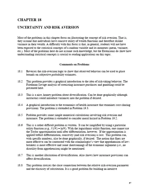
CHAPTER 18UNCERTAINTY AND RISK AVERSIONMost of the problems in this chapter focus on illustrating the concept of risk aversion. That is, they assume that individuals have concave utility of wealth functions and therefore dislike variance in their wealth. A difficulty with this focus is that, in general, students will not have been exposed to the statistical concepts of a random variable and its moments (mean, variance, etc.). Most of the problems here do not assume such knowledge, but the Extensions do show how understanding statistical concepts is crucial to reading applications on this topic.Comments on Problems18.1 Reverses the risk-aversion logic to show that observed behavior can be used to placebounds on subjective probability estimates.18.2 This problem provides a graphical introduction to the idea of risk-taking behavior. TheFriedman-Savage analysis of coexisting insurance purchases and gambling could bepresented here.18.3 This is a nice, homey problem about diversification. Can be done graphically althoughinstructors could introduce variances into the problem if desired.18.4 A graphical introduction to the economics of health insurance that examines cost-sharingprovisions. The problem is extended in Problem 19.3.18.5 Problem provides some simple numerical calculations involving risk aversion andinsurance. The problem is extended to consider moral hazard in Problem 19.2.18.6 This is a rather difficult problem as written. It can be simplified by using a particularutility function (e.g., U(W) = ln W). With the logarithmic utility function, one cannot use the Taylor approximation until after differentiation, however. If the approximation isapplied before differentiation, concavity (and risk aversion) is lost. This problem can,with specific numbers, also be done graphically, if desired. The notion that fines aremore effective can be contrasted with the criminologist’s view that apprehension of law-breakers is more effective and some shortcomings of the economic argument (i.e., nodisutility from apprehension) might be mentioned.18.7 This is another illustration of diversification. Also shows how insurance provisions canaffect diversification.18.8 This problem stresses the close connection between the relative risk-aversion parameterand the elasticity of substitution. It is a good problem for building an intuitive9798 Solutions Manualunderstanding of risk-aversion in the state preference model. Part d uses the CRRAutility function to examine the “equity-premium puzzle.”18.9 Provides an illustration of investment theory in the state preference framework.18.10 A continuation of Problem 18.9 that analyzes the effect of taxation on risk-takingbehavior.Solutions18.1 p must be large enough so that expected utility with bet is greater than or equal to thatwithout bet: p ln(1,100,000) + (1 –p)ln(900,000) > ln(1,000,000)13.9108p +13.7102(1 –p) > 13.8155, .2006p > .1053 p > .52518.2This would be limited by the individual’s resources: he or she could run out of wealth since unfair bets are continually being accepted.18.3 a.Strategy One Outcome Probability12 Eggs .50 Eggs .5Expected Value = .5∙12 + .5∙0 = 6Strategy Two Outcome Probability12 Eggs .256 Eggs .50 Eggs .25Expected Value = .25 ∙12 + .5 ∙ 6 + .25∙ 0= 3 + 3 = 6Chapter 18/Uncertainty and Risk Aversion 99b.18.4 a. E(L) = .50(10,000) = $5,000, soWealth = $15,000 with insurance, $10,000 or $20,000 without.b. Cost of policy is .5(5000) = 2500. Hence, wealth is 17,500 with no illness, 12,500with the illness.18.5 a. E(U) = .75ln(10,000) + .25ln(9,000) = 9.1840b. E(U) = ln(9,750) = 9.1850 Insurance is preferable.c. ln(10,000 – p ) = 9.184010,000 – p = e 9.1840 = 9,740p = 26018.6 Expected utility = pU(W – f) + (1 – p)U(W). ,[()()]/U p U pU W f U W p U e p U∂=⋅=--⋅∂,()/U f U fp U W f f U e f U∂'=⋅=-⋅-⋅∂100 Solutions Manual,,()()1()U p U fU W f U W e f U W f e --=<'-- by Taylor expansion,So, fine is more effective.If U (W ) = ln W then Expected Utility = p ln (W – f ) + (1 – p ) ln W .,/[ln ()ln ]U pp p f WW f W e U U -=--⋅≈ ,/()/()U ff p f W f p U W f e U U--=--⋅= ,,1U p U fW fe W e -=<18.7 a. U (wheat) = .5 ln(28,000) + .5 ln(10,000) = 9.7251 U (corn) = .5 ln(19,000) + .5 ln(15,000) = 9.7340 Plant corn. b. With half in eachY NR = 23,500Y R = 12,500U = .5 ln(23,500) + .5 ln(12,500) = 9.7491Should plant a mixed crop. Diversification yields an increased variance relative to corn only, but takes advantage of wheat’s high yield.c. Let α = percent in wheat. U = .5 ln[ (28,000) + (1 – α )(19,000)] + .5 ln[α (10,000) + (1 – α )(15,000)] = .5 ln(19,000 + 9,000α) + .5 ln(15,000 – 5,000α)45002500019,0009,00015,0005,000dU d ααα=-=+- 45(150 – 50α) = 25(190 + 90α) α = .444 U = .5 ln(22,996) + .5 ln(12,780) = 9.7494. This is a slight improvement over the 50-50 mix. d. If the farmer plants only wheat,Y NR = 24,000Y R = 14,000U = .5 ln(24,000) + .5 ln(14,000) = 9.8163so availability of this insurance will cause the farmer to forego diversification.Chapter 18/Uncertainty and Risk Aversion 10118.8 a. A high value for 1 – R implies a low elasticity of substitution between states of theworld. A very risk-averse individual is not willing to make trades away from the certainty line except at very favorable terms.b. R = 1 implies the individual is risk-neutral. The elasticity of substitution between wealth in various states of the world is infinite. Indifference curves are linear with slopes of –1. If R =-∞, then the individual has an infinite relative risk-aversion parameter. His or her indifference curves are L-shaped implying an unwillingness to trade away from the certainty line at any price.c. A rise in b p rotates the budget constraint counterclockwise about the W g intercept. Both substitution and income effects cause W b to fall. There is a substitution effect favoring an increase in W g but an income effect favoring a decline. The substitution effect will be larger the larger is the elasticity of substitution between states (the smaller is the degree of risk-aversion).d. i. Need to find R that solves the equation:R R R W W W )955.0(5.0)055.1(5.0)(000+=This yields an approximate value for R of –3, a number consistent with some empirical studies.ii. A 2 percent premium roughly compensates for a ±10 percent gamble. That is:303030)12.1()92(.)(---+≈W W W .The “puzzle” is that the premium rate of return provided by equities seems to be much higher than this.18.9 a. See graph.Risk free option is R , risk option is R '. b. Locus RR' represents mixed portfolios.c. Risk-aversion as represented by curvature of indifference curves will determine equilibrium in RR' (say E ).102 Solutions Manuald. With constant relative risk-aversion, indifference curve map is homothetic so locus ofoptimal points for changing values of W will be along OE.18.10 a. Because of homothetic indifference map, a wealth tax will cause movement along OE(see Problem 18.9).b. A tax on risk-free assets shifts R inward to Rt (see figure below). A flatter RR t'provides incentives to increase proportion of wealth held in risk assets, especially for individuals with lower relative risk-aversion parameters. Still, as the “note” implies, it is important to differentiate between the after tax optimum and the before taxchoices that yield that optimum. In the figure below, the no-tax choice is E on RR'.* EW represents the locus of points along which the fraction of wealth held in risky assets is constant. With the constraint RR t' choices are even more likely to be to the right of EW* implying greater investment in risky assets.c. With a tax on both assets, budget constraint shifts in a parallel way to RR tt'. Even in this case (with constant relative risk aversion) the proportion of wealth devoted to risky assets will increase since the new optimum will lie along OE whereas a constant proportion of risky asset holding lies along EW O.103。
资产定价经典文献总结一、理论部分(一)开山之作Bachelier, L.,1900,1964, “Theory of Speculation, in P. Cootner (ed.)”, The Random Character of Stock Market Prices, Cambridge, MA:MIT Press, pp.17~78.(二)一般均衡理论1、Arrow, Kenneth, and Gerard Debreu, 1954, “Existence of an Equilibri um fora Competitive Economy,” Econometrica 22, 265–290.(三)证券组合选择理论1、Markowitz, M., 1952,“Portfolio Selection”, Journal of Finance, 7(1), pp.77~91.(提出最优投资组合模型,以资产回报率的均值和方差作为选择的对象,不考虑个体的效用函数)2、Jaganmatham, B. and T. Ma , 2002,“Risk Reduction in Large Portfolios: A Role for Portfolio Weight Constraints”,Working Paper, Northwestern University.(研究投资组合权重受限制时的最优投资组合问题)(四)资本资产定价理论1、Sharpe, W., 1964,“Capital Asset Prices: A Theory of Capital Market Equilibrium under Conditions of risk”, Journal of Finance, 19, pp.425~442.2、Lintner, L., 1965,“The Valuation of Risk Assets and the Selection of Risky Investments in Stock Portfolios and Capital Budgets”, Review of economics and Statistics, 47, pp.13~37.3、Mossin, J., 1965, “Equilibrium in a Capital Asset Market”, Econometrica, 35, pp.768~783.(以上三篇文献独立地得出资本资产定价理论)4、Fama, E. and K. French, 2004, “The Capital Asset Pricing Model: Theory and Evidence”, Working paper.(对CAPM的理论和实证研究作了综述性描述)(五)期权定价理论1、Sharpe, W., 1978, Investments, Englewood Cliffs, NJ:Prentice- Hall.(衍生证券定价理论之一:二叉树模型)2、Cox, J., S. Ross and M. Rubinstein, 1979, “Option Pricing: A Simplified Approach”, Journal of Financial Economics,7 , pp.229~63.(对二叉树模型的扩展;二叉树的数值算法)3、Black, F. and M. Scholes, 1973, “The Pricing of Options and Corporate Liabilities”, Journal of Political Economy, 81 (3), pp.637~654.4、Merton, R., 1973a,“Theory of Rational Option Pricing”,Bell Journal of Economics and Management Sciences, 4(1),pp.141~183.(衍生证券定价之二:连续时间模型,利用随机分析第一次对期权定价问题提出了严格的解决方法——偏微分方程法)5、Smith, C, 1976,“Option Pricing: A Review”, Journal of Financial Economics, 3, pp.3~51.6、Malliaris, A., 1983 ,“Ito' s Calculus in financial Decision Making”, Society of Industrial and Applied Mathematics Review, 25, pp.481~496.(给出了偏微分方程的具体解过程)7、Duffie, D. J., 1992, “Dynamic Asset Pricing Theory”,Princeton University Press,Princeton.(给出了BSM定价公式的数学基础以及金融解释,同时还给出了期权定价的金融解释)8、Merton, R., 1997, “Applications of Option –pricing Theory: Twenty- five Years Later”,American Economic Review, 88(3), pp.323~349.9、Scholes, M, 1997,“Derivatives in a Dynamic Environment”,American Economic Review, 88(3), pp.350~370.(两位学者在诺贝尔奖大会上对过去30年相关领域的发展回顾)10、Cox, J. and S. Ross, 1976, “The Valuation of Options for Alternative Stochastic Processes”,Journal of Financial Economics, 3, pp.145~66.(衍生证券定价之三:风险中性定价模型,引入了风险中性定价的概念)11、Harrison, J. and D. Kreps, 1979,“Martingales and Arbitrage in Multi - period Securities Markets”, Journal of Economic Theory, 20, pp.381~408.12、Harrison, J. and S. Pliska, 1981, “Martingale and Stochastic Integrals in the Theory of Continuous Trading”,Stochastic Process, Appl., 11, pp.215~260.(建立了系统的风险中性定价理论框架以及市场无套利在其中的表现形式)13、Geman, H., N. El Karoui and J. Rochet, 1995,“Changes of Numeraire, Changes of Probability Measures and Pricing of Options”, Journal of Applied Probability, 32, pp.443~458.(早期的风险中性定价是以货币市场帐户为计量单位的,该文章认为我们可以选取不同的计量单位,对于每一个计量单位,都有一个概率与其相对应,从而有不同的定价模型)14、Roll, R., 1977,“An Analytical Formula for Unprotected American Call Options on Stocks with Known Dividends”,Journal of Financial Economics, 5, pp.251~258.(美式期权与奇异期权定价之一:近似算法。
国际金融普通高等教育“十一五”国家级规划教材国家级精品课程教材第三章汇率制度和外汇管制学习要求通过本章的学习,要求掌握汇率制度的概念及其分类,关于固定和浮动汇率制度孰优孰劣的传统争论,货币局制度的特点及其风险与收益,联系汇率制的运行机制,货币替代以及美元化的概念,外汇管制的概念、方式以及成本和收益分析,我国现阶段的外汇管理和人民币汇率状况。
引导同学运用汇率制度和外汇管制的相关理论对现实问题进行分析,以正确看待目前世界各国汇率制度选择和外汇管制问题。
学习要点第一节汇率制度第二节货币局制度和美元化第三节外汇管制第四节我国外汇管理体制和人民币汇率制度改革第一节汇率制度一.汇率制度(Exchange Rate Regime/System):又称汇率安排(Exchange Rate Arrangement),是指一国货币当局对本国汇率确定和调整的基本原则和方式所做出的一系列规定或安排。
传统上,根据有没有规定货币平价以及汇率波动幅度的大小,汇率制度可划分为固定汇率制和浮动汇率制两大类。
二.汇率制度的分类(一)固定汇率制固定汇率制(Fixed Exchange Rate System),是指本币对外币规定有货币平价,现实汇率受货币平价制约,只能围绕平价在很小的范围内波动的汇率制度。
自19世纪中末期金本位制在西方各主要资本主义国家确定以来,一直到1973年,世界各国的汇率制度基本上都属于固定汇率制。
第一节汇率制度固定汇率制度包括金本位制下的固定汇率和纸币流通条件下的固定汇率,发展过程经历了两个阶段:一是从1816年到第二次世界大战前的国际金本位制度时的固定汇率制;二是从第二次世界大战后到1973年布雷顿森林体系下的固定汇率制。
这两种汇率制度的共同点是:①各国对本国货币都规定有金平价,中心汇率是按两国货币各自的金平价之比来确定的。
②外汇市场上的汇率水平相对稳定,围绕中心汇率在很小的范围内波动。
第一节汇率制度不同点:①金本位制下的固定汇率制是自发形成的;而在布雷顿森林体系下,固定汇率制是通过国际间的协议人为建立起来的。
第三章 效用论3.1效用论概述 3.1.1效用的概念效用(Utility ):消费者从消费某种物品中所得到的满足程度。
(注:主观感受或主观评价。
)3.1.2 基数效用和序数效用3.1.3 基数效用论和边际效用分析法1.边际效用递减规律(Diminishing Return of MU )(1) 总效用(TU :Total Utility ):消费者消费一定量某种物品所得到的总的满足程度。
(2) 边际效用(MU: Marginal Utility ):消费者增加一单位某种物品消费所增加的总效用。
QQ TU MU ∆∆=)(()dQQ dTU QQ TU MU Q =∆∆=→∆)(lim(3) 边际效用递减规律:在一定时间内,在其他商品的消费数量保持不变的条件下,随着消费者对某种商品消费量的增加,消费者从该商品增加的每一消费单位中所得到效用增量即边际效用是递减的。
2.关于货币的边际效用:符合边际效用递减规律,但递减速度较慢,因此,通常假设为常数。
3.基数效用论下的消费者均衡(1)消费者均衡含义:研究单个消费者如何把有限的货币收入分配在各种商品的购买中以获得最大的效用。
即,研究单个消费者在既定收入下实现效用最大化的均衡条件。
(2)消费者均衡条件目标函数:)....,(21n X X X MaxTU约束条件:n n X P X P X P M ∙++∙+∙= 2211 均衡条件mnnMUP MU P MU P MU ==== 2211 或 miiMUP MU = (i=1,2,…,n )4.基数效用论下需求曲线的推导(1)商品的需求价格是指消费者在一定时期内对一定量的某种商品所愿意支付的最高价格。
基数效用论者认为,商品的需求价格取决于商品的边际效用。
(2)推导需求曲线即是说明价格和需求量间的反比关系,进而解释需求曲线向右下方倾斜的原因。
5.消费者剩余(CS ,Consumer Surplus )(1)含义:消费者在购买一定数量某商品时愿意支付的最高总价格和实际支付的总价格之间的差异。
正确认识确定感与自主感导语:世界唯一不变的是变化,中国企业尤甚。
经济快速发展、竞争日益加剧、组织变革频频、制度朝令夕改、领导经常更替都严重挑战着员工的确定感和自主感。
而心理学和脑科学的研究显示,满足员工确定感和自主性需求,能提升他们的幸福感、健康水平、工作成果。
2001年9月11日,对于美国人来说是一个惨痛的日子,而对于美国航空业来说,更是意味着双重的不幸。
在事件发生之后的数天之内,由于航空管制所带来的经济压力使得原本就已疲乏的航空业雪上加霜。
很快,几乎所有航空公司都做出了共同的应对政策:裁员。
在这一波数以万计的裁员浪潮中,只有一家航空公司不为所动。
不仅如此,第二年的2月,这家公司更逆潮流而上,宣布了一项4000人的增员计划。
这家航空公司就是当前美国国内航空的第一大运营商——西南航空。
他们坚持自己的“不裁员”政策已经数十年,甚至在2011年兼并了穿越航空公司之后,他们马上做出的宣布就是:不会裁员。
与此同时,在美国航空业的一片愁云惨雾中,西南航空却依然“这边风景独好”,一直保持着较为健康的收支平衡。
当面临着严峻的经济形势,对于大多数企业领导者来说,跃进脑海的第一个念头往往就是:裁员。
在他们看来,只有通过裁员才能迅速降低企业的经济负担,以便为经济复苏时的重振做出准备。
然而,科罗拉多大学一项持续18年的研究指出,经常采取裁员政策的企业往往既不能削减支出,也不能增加收益,难以实现迅速的经济成长。
在裁员政策与企业利润之间到底存在什么样的关联?从神经领导力的角度来看,在一家动不动就裁员的企业中,员工不仅会失去对工作的确定感,同时也会觉得自己无法控制生活。
为此,在对地位感与公平感进行探讨之后,我们将继续探讨另外两项影响员工的社会需要:确定感与自主感。
在本文中,我们所探讨的确定感指个体对于自己行为或决定结果的清楚认识,自主感则是个体可以控制其生活,或者影响其环境的感受。
我们希望企业领导者意识到,确定感与自主感并不只是与裁员这样的战略性决策有关,更体现在企业日常管理的方方面面,涵盖于领导者与员工的日常社会交往中。
Uncertainty Aversion with Second-Order Probabilities and UtilitiesRobert F. NauFuqua School of BusinessDuke University/~rnauRUD 2002 versionMay 21, 2002AbstractUncertainty aversion is often conceived as a local, first-order effect that is associated with kinked indifference curves (i.e., non-smooth preferences), as in the Choquet expected utility model. This paper shows that uncertainty uncertainty aversion can arise as a global, second-order effect when the decision maker has smooth preferences within the state-preference framework of choice under uncertainty, as opposed to the Savage or Anscombe-Aumann frameworks. Uncertainty aversion is defined and measured in direct behavioral terms without reference to probabilistic beliefs or consequences with state-independent utility. A simple axiomatic model of “partially separable” non-expected utility preferences is presented, in which the decision maker satisfies the independence axiom selectively within partitions of the state space whose elements have similar degrees of uncertainty. As such, she may behave like an expected-utility maximizer with respect to assets in the same uncertainty class, while exhibiting higher degrees of risk aversion toward assets that are more uncertain. An alternative interpretation of the same model is that the decision maker may be uncertain about her credal state (represented by second-order probabilities for her first-order probabilities and utilities), and she may be averse to that uncertainty (represented by a second-order utility function). The Ellsberg and Allais paradoxes are explained by way of illustration. Keywords: risk aversion, uncertainty aversion, ambiguity, non-additive probabilities, state-preference theory, Choquet expected utility, Ellsberg’s paradox.1. IntroductionThe axiomatization of expected utility by von Neumman-Morgenstern and Savage hinges on the axiom of independence, which requires preferences to be separable across mutually exclusive events and leads to representations by utility functions that are additively separable across states of the world. A strong implication of the independence axiom is that preferences among acts do not depend on qualitative properties of events but rather only on the sum of the values attached to their constituent states, which in turn depend only on the probabilities of the states and the consequences to which they lead. If the set of states of nature can be partitioned in two or more ways, the decision maker is not permitted to display uniformly different risk attitudes toward acts that are measurable with respect to different partitions, because the events in any two partitions are composed of the same states, merely grouped in different ways. There is considerable empirical evidence that individuals violate this requirement in certain kinds of choice situations. One example is provided by Ellsberg’s 2-color paradox, in which subjects consistently prefer to bet on unambiguous events rather than ambiguous events, even when they are otherwise equivalent by virtue of symmetry, a phenomenon known as uncertainty aversion. Other violations of independence are provided by Ellsberg’s 3-color paradox and Allais’ paradox, in which subjects’ preferences between two acts that agree in some events depend on how they agree there, as though there were complementarities among events.A variety of models of non-expected utility have been proposed to accommodate violations of the independence axiom, and most of them do so by positing that the decision maker has non-probabilistic beliefs or that her preferences depend nonlinearly on probabilities. The Choquet expected utility model, in particular, assumes that the decision maker tends to overweight events leading to inferior payoffs by applying non-additive subjective probabilities derived from a Choquet capacity. (Schmeidler 1989) The ranking ofstates according to the payoffs to which they lead thus plays a key role in the representation of uncertainty aversion: the decision maker violates the axioms of expected utility theory only when faced with choices among acts whose payoffs induce different rankings of states. Within sets of acts whose payoffs are comonotonic, the decision maker’s preferences have an ordinary expected-utility representation. Schmeidler derives the Choquet model within the Anscombe-Aumann framework of choice under uncertainty, which includes objective probabilities in the composition of acts, and he defines uncertainty aversion in this framework as convexity with respect to mixtures of probabilities. That is, an uncertainty-averse individual who prefers f to g also prefers αf+ (1−α)g to g for 0<α<1,where the mixture operation applies to the objective probabilities with which acts f and g lead to various consequences. Another way to view the Choquet model is to note that it implies that the decision maker has indifference curves in payoff space that are kinked in particular locations, namely at the boundaries between comonotonic sets of acts. If the decision maker’s status quo wealth happens to fall on such a kink—which is a set of measure zero—her local preferences (i.e., her preferences for “neighboring” acts) will display uncertainty aversion, otherwise they will not.Epstein (1999) takes a different approach, in which uncertainty aversion is defined as a departure from probabilistically sophisticated behavior (Machina and Schmeidler 1992). A probabilistically sophisticated decision maker may have non-expected-utility preferences but nevertheless has an additive subjective probability measure that is uniquely determined by preferences. Epstein (following Machina and Schmeidler) uses the Savage-act modeling framework, in which objects of choice are mappings from states to consequences whose utilities are a priori state-independent. There are no objectively mixed acts; rather, Epstein’s definition of uncertainty aversion assumes the existence of a set of special acts that are a priori unambiguous. A preference order 1! is defined to be more uncertainty averse thanpreference order 2! if, for all acts w and all unambiguous acts y, y1!w(y1!w) whenever y2!w( y 2!w). In other words, order 1 is more uncertainty averse than order 2 if 1 never chooses an ambiguous act over an unambiguous act when 2 would not. A preference order is then defined to be uncertainty averse if it is more uncertainty averse than some probabilistically sophisticated preference order. Epstein and Zhang (2001) extend the same approach to define the set of unambiguous events endogenously: an unambiguous event is one that does not give rise to preference reversals when a common consequence assigned to that event is replaced by another common consequence.Ghirardato and Marinacci (2001, 2002) give a definition of uncertainty aversion that, like Epstein’s, is based on a definition of comparative uncertainty aversion but is more general in the sense that it does not assume the existence of acts that are a priori unambiguous, aside from the constant acts that play a key role in Savage’s framework. However, Ghirardato and Marinacci’s definition imposes the additional restriction that preferences should be biseparable—i.e., that when choices are restricted to binary gambles, preferences should be represented by a utility function of the form V(xAy) =u(x)ρ(A) + u(y)(1−ρ(A)), where u is a cardinal utility function for money and ρ is a “willingness to bet”measure. Uncertainty aversion is exhibited when ρ is nonadditive, i.e., ρ(A)+ρ(A) < 1.The preceding definitions of uncertainty aversion are motivated by the Choquet expected utility model and related models in which uncertainty aversion is associated with kinked indifference curves—thus, uncertainty aversion is conceived as a first-order rather than second-order effect (Segal and Spivak 1990)—and they all require a priori definitions of riskless (constant) acts in the tradition of Savage and Anscombe-Aumann. The aim of the present paper is to consider, instead, situations in which (i) there are no a priori riskless acts or consequences whose utilities are state-independent, (ii) the decision maker has smooth preferences so that both risk aversion and uncertainty aversion are second-order effects, and(iii) the decision maker may be locally uncertainty averse at all wealth positions, not merely at “special” wealth positions. The definition of uncertainty aversion given here is somewhat similar in spirit to that of Ghirardato and Marinacci, insofar a decision maker is considered uncertainty averse if she is “more uncertainty averse” than a decision maker with separable preferences. However, unlike Schmeidler, Epstein, and Ghirardato/Marinacci, we make no attempt to uniquely separate beliefs from state-dependent cardinal utilities, on the grounds that such a separation is impossible to achieve in practice and is not necessary for purposes of economic modeling or decision analysis (Nau 2002). Roughly speaking, a decision maker will be defined here to be uncertainty averse if she is systematically more risk averse toward acts that are “more uncertain” in a manner that cannot be explained by a state-dependent Pratt-Arrow measure of risk aversion. For example, she might be risk neutral—or even locally risk seeking—toward casino gambles, moderately risk averse toward investments in the stock market, and highly risk averse when insuring against health or property risks.The organization of the paper is as follows. Section 2 introduces the basic mathematical framework, and section 3 defines risk aversion and uncertainty aversion for a decision maker with smooth preferences. Section 4 gives a simple example of a utility function defined on a 4-element state space that rationalizes Ellsberg’s 2-color paradox. Section 5 presents a more detailed and general version of the same model and the axioms of “partially separable preferences” on which it rests. Section 6 presents an alternative interpretation of the model in terms of second-order uncertainty about credal states, illustrated by a model of Ellsberg’s 3-color paradox as well as the 2-color paradox. Section 7 presents two different models for the Allais paradox, one that is based on second-order uncertainty about probabilities and another that is based on second-order uncertainty about utilities. Section 8 discusses how the preference model differs from Choquet expected utility, and Section 9 presents some concluding comments.2. PreliminariesThe modeling framework used throughout this paper is that of state-preference theory (Arrow 1953/1964, Debreu 1959, Hirshleifer 1965), which encompasses both expected-utility and non-expected-utility models of choice under uncertainty.1 Suppose that there are n mutually exclusive, collectively exhaustive, states of nature and a single divisible commodity (money) in terms of which payoffs are measured. The wealth distribution of a decision maker is represented by a vector w ∈ ℜn , whose j th element w j denotes the quantity of money received in state j , in addition to (unobserved) status quo wealth.Assumption 1: The decision maker’s preferences among wealth distributions satisfy the usual axioms of consumer theory (reflexivity, completeness, transitivity,continuity, and monotonicity), as well as a smoothness property, so that they are representable by a twice-differentiable ordinal utility function U (w ) that is a non-decreasing function of wealth in every state.By the monotonicity assumption, the gradient of U at wealth w is a non-negative vector that can be normalized to yield a probability distribution π(w ) whose j th element is∑=∂∂∂∂=n i i jj w U w U 1)/()/()(w w w π.Thus, πj (w ) is the rate at which the decision maker would indifferently bet infinitesimal amounts of money on or against the occurrence of state j .2 π(w ) is invariant to monotonic1 For our purposes, the appeal of the state-preference framework is that it uses concrete sums of money as outcomes without necessarily assuming that utility for money is state-independent or that background wealth is observable or that utilities and subjective probabilities are uniquely separable.2 Because preferences are assumed to be both complete and smooth, we rule out first-order aversion to risk or uncertainty, in which, even for infinitesimal stakes, there might be no rate at which the decision maker would indifferently bet on or against a given event.transformations of U and is observable, regardless of whether the decision maker is probabilistically sophisticated. It is commonly known as a risk neutral probability distribution because the decision maker prices very small assets in a seemingly risk-neutral manner with respect to it. A state will be defined here to be non-null if its risk neutral probability is positive at every wealth distribution. A decision maker’s risk neutral probabilities at wealth w are implicitly a function of her beliefs, her attitudes toward risk and uncertainty, and her personal and financial stakes in events, although their effects are often confounded.The risk-neutral distribution π(w ) describes the first-order properties of the decision maker’s local preferences in the vicinity of wealth w . Second-order properties of local preferences are described by the matrix R (w ) whose jk th element isj kj jk w U w w U r ∂∂∂∂∂−=)/()/()(2w w w .R (w ) generalizes the familiar Pratt-Arrow measure to the present setting and will be called the risk aversion matrix . Hence, the decision maker’s local preferences at wealth w are described, up to second-order effects, by a risk neutral probability distribution π(w ) and a risk aversion matrix R (w ).3If no additional restrictions are placed on preferences, the individual is rational by the standard of no-arbitrage, but she may have non-expected utility preferences in the sense that3 The matrix R (w ) is not observable in the general case, just as the ordinal utility function U is not observable.U is determined by preferences only up to monotonic transformations, and correspondingly R (w ) is uniquely determined by preferences only up to the addition of constants to each column. However, R (w ) can benormalized subtracting a constant from each column so that the risk neutral expectation of each column is zero,and the normalized matrix is observable. (Nau 2001) Here the “unnormalized” matrix R (w ) will be used for convenience, but the results could as well be recast in terms of the normalized matrix.her valuation of a risky asset may not be decomposable into a product of probabilities for states and utilities for consequences. For example, she may behave as if amounts of money received in different states are substitutes or complements for each other, which is forbidden under expected utility theory. However, if her preferences are additionally assumed to satisfy the independence axiom (Savage’s P2), then U(w) has an additively separable representation: U(w) = v1(w1) + v2(w2) + … + v n(w n).In this case, R(w) reduces to an observable diagonal matrix. If preferences are further assumed to be conditionally state-independent (Savage’s P3), then U(w) has a state-independent expected-utility representation:U(w) = p1u(w1) + p2u(w2) + … + p n u(w n),where p is a unique probability distribution and u(x) is a state-independent utility function that is unique up to positive affine scaling, as in Savage’s model.4 Although the probabilities in the latter representation are unique, it does not yet follow that they are the decision maker’s “true” subjective probabilities, because there are many other equivalent representations in which different probabilities are combined with state-dependent utilities. In order for the decision maker to be probabilistically sophisticated—i.e., in order for her preferences to determine a unique ordering of events by probability—an additional qualitative probability axiom (Savage’s P4 or Machina and Schmeidler’s P4*, 1992) is needed, together with an a priori definition of consequences whose utility is “constant”4 For a decision maker who is a state-independent expected-utility maximizer, risk neutral probabilities are merely the product of true subjective probabilities and relative marginal utilities for money at the current wealth position, i.e., πj(w) ∝p j u′(w j), where p j is the subjective probability of state j and u(w) is the state-independent utility of wealth w. If an attempt is made to elicit the decision maker’s subjective probabilities by de Finetti’s method—i.e., by asking which gambles she is willing to accept—the probabilities that are observed will be her risk neutral probabilities rather than her true probabilities.across states of nature. However, preference measurements among feasible acts do not reveal whether the consequences are, in fact, constant, and so the unique separation of probability from cardinal utility remains problematic and controversial (Schervish et al. 1990, Karni and Mongin 2000, Karni and Grant 2001, Nau 2002, Karni 2002). For this reason, it is of interest to try to define both risk aversion and uncertainty aversion in a way that does not depend on the a priori identification of a set of constant consequences nor on the assumption of state-independent preferences.53. Definitions of aversion to risk and uncertaintyIn order to characterize aversion to uncertainty, it is necessary to begin with a characterization of aversion to risk. Following Yaari (1969) the decision maker is defined to be risk averse if her preferences are convex with respect to mixtures of payoffs, which means that whenever w is preferred to w*, αw+(1−α)w* is also preferred to w* for 0<α<1, where αw+(1−α)w*denotes the wealth distribution whose monetary value in state i is αw i+(1−α)w i*.6 Payoff-convexity of preferences implies that the ordinal utility function U is quasi-concave. This definition of risk aversion does not require prior definitions of expected value or absence of risk.7 The decision maker’s degree of local risk aversion can be5 Epstein and Zhang (2001) explicitly invoke Savage’s state-independent utility axiom (P3) and observe: “The necessity of this axiom in our approach implies, in particular, that we have nothing to say about the meaning of ambiguity when preferences are state-dependent.” [p. 275, emphasis added]6 Note that there is a suggestive duality between Yaari’s definition of risk aversion as payoff-convexity and Schmeidler’s definition of uncertainty aversion as probability-convexity. However, Schmeidler’s definition is criticized by Epstein (1999) and cannot be applied in the present framework, which lacks objective probabilities.7 See Machina (1995) and Karni (1995) for a discussion of the implications of different definitions of risk aversion under non-expected utility preferences.measured by the difference between her risk-neutral valuation of an asset and the price at which she is actually willing to buy it. Let z denote the payoff vector of a risky asset. The decision maker’s buying price for z at wealth w, denoted B(z;w), is determined by U(w+z–B(z;w)) −U(w) = 0.The (buying) risk premium associated with z at wealth w,here denoted b(z;w), is the difference between the asset’s risk neutral expected value and its buying price: b(z;w) = Eπ(w)[z] – B(z;w).It follows (as a consequence of quasi-concavity) that the decision maker is risk averse if and only if her risk premium is non-negative for every asset z at every wealth distribution w.If z is a neutral asset (Eπ(w)[z] = 0), its risk premium has the following second-order approximation that generalizes the Pratt-Arrow formula (Nau 2001):b(z;w) ≈ ½ z T Π(w)R(w) z,where Π(w)= diag(π(w)). In the special case where U is additively separable (i.e., the decision maker satisfies the independence axiom), R(w)is an observable diagonal matrix and the risk premium formula reduces tob(z;w) ≈ ½ Eπ(w)[r(w)z2],where r(w) is a vector-valued risk aversion measure whose j th element isr j(w) = −U jj(w)/U j(w).Hence, for a decision maker with quasi-concave additively-separable utility, local preferences are completely described (up to second-order effects) by a pair of numbers for each state: a risk neutral probability πj(w) and a risk aversion coefficient r j(w). Such a decision maker is risk averse but uncertainty neutral, inasmuch as her preferences have an expected-utility representation even if her probabilities cannot be uniquely separated from her (possibly state-dependent) utilities.It remains to characterize aversion to uncertainty in a simple behavioral way. For convenience, in the spirit of Epstein (1999), we assume that there is a reference set of events that are a priori “unambiguous.”8Assumption 2: There is a set of unambiguous events, closed under complementation and disjoint union, at least one of which is a union of two or more non-null states and whose complement is also a union of at two or more non-null states.Intuitively, a decision maker is averse to uncertainty if she prefers to bet on unambiguous rather than ambiguous events, other things being equal. To make this notion precise, we introduce the notion of an A:B ∆-spread (“A vs. B delta-spread”). Let A and B denote two logically independent events, let {AB π,B A π,B A π,B A π}denote the local risk neutral probabilities (at wealth w ) of the four possible joint outcomes of A and B , and assume they are all strictly positive. Let ∆ denote a quantity of money (just) large enough in magnitude that second-order utility effects are relevant. Then an A:B ∆-spread and a B:A ∆-spread are defined as the neutral assets whose payoffs are given by the following two contingency tables:B B AA A A Table 1: ∆-spreads defined8 The unambiguous events play no essential role in the analysis except to distinguish whether a particular pattern of behavior is ambiguity-averse or ambiguity-loving. Since unambiguous events can be created if necessary by flipping coins, this entails no great loss of generality. However, we do not assume that unambiguous events necessarily have have objective or otherwise uniquely determined probabilities.Note that an A:B ∆-spread is a non-simple bet on A: the sign of the payoff depends only on whether A occurs or not, but the magnitude may also depend on B. Similarly, a B:A ∆-spread is a non-simple bet on B whose payoff magnitude may depend on A. In both cases, the winning and losing amounts are scaled so that the contribution to the risk neutral expected payoff is ±∆ in every cell of the table. By construction, both bets are neutral and both must have the same risk premium for a decision maker with separable preferences, because for such a person the risk premium is obtained (to a second order approximation) by squaring the payoffs, multiplying them by the statewise risk neutral probabilities and risk aversion coefficients, and summing.Definition 1: The decision maker is locally uncertainty averse at wealth w if, forevery unambiguous event B, every event A that is logically independent of B, and any ∆ sufficiently small in magnitude (positive or negative), a B:A ∆-spread is weaklypreferred to (i.e., has a risk premium less than or equal to that of) an A:B ∆-spread.The decision maker is uncertainty averse if she is locally uncertainty averse at every wealth position.The classic demonstration of uncertainty aversion is provided by Ellsberg’s 2-color paradox, in which a subject prefers to stake a modest prize (say, $400) on the draw of a ball from an urn with equal proportions of red and black balls rather than a draw from an urn with unknown proportions of red and black, regardless of the winning color. To adapt this experiment to the framework of Definition 1, let B denote the unambiguous event that a red ball is drawn from urn 1 (with known 50-50 proportions of red and black) and let A denote the potentially ambiguous event that a red ball is drawn from urn 2 (with unknown proportions of red and black). By symmetry, if there are no prior stakes, it is reasonable to suppose that the decision maker’s risk neutral probabilities for the four possible joint outcomes are identically 1/4. Then, according to Definition 1, an uncertainty averse decisionmaker would prefer to receive +4∆ in the event that red is drawn from urn 1 and −4∆ in the event that black is drawn from urn 1 (a B:A ∆-spread ) rather receive +4∆ in the event that red is drawn from urn 2 and −4∆ in the event that black is drawn from urn 2 (an A:B ∆-spread), regardless of whether ∆ is +$100 or −$100.In Ellsberg’s three-color paradox, there is a single urn containing 30 red balls and 60 balls that are black and yellow in unknown proportions. A typical subject prefers to stake (say) a $300 prize on the draw of a red ball rather than a black ball when $0 is to be received in either case if a yellow ball is drawn, but the direction of preference is reversed when $300 is to be received if yellow is drawn. The 3-color paradox is more transparently a violation of the independence axiom but less transparently an example of aversion to uncertainty. It is usually presented as a set of choices among prospects that involve only gains:a b c d e fRed300000300300Black030003000300Yellow003003003000Table 2: Ellsberg’s 3-color paradox in gains-only formThe typical response pattern is a > b ~ c and d > e ~ f. When the prospects are converted to “fair” gambles by subtraction of appropriate constants, the choices look like this:a′b′c′d′e′f′Red200-100-100-200100100Black-100200-100100-200100Yellow-100-100200100100-200Table 3: Ellsberg’s 3-color paradox in fair-gamble formThe last three gambles are merely the opposite sides of the first three. We would expect an uncertainty-averse subject to give the same pattern of responses, i.e., a′ > b′ ~ c′ and d′ > e′ ~ f′, and indeed the Choquet expected utility model predicts exactly this result. However, a′ >b′ ~ c′ and d′ > e′ ~ f′ does not violate the independence axiom. For example, it is consistent with a model of state-dependent expected-utility preferences of the following form: U(w) = ⅓( −2 exp(−½ αw1)) + ⅓(−exp(−αw2)) + ⅓(−exp(−αw3)),where w1, w2, w3 are the amounts of wealth received under Red, Black, and Yellow, respectively, and α is any positive number. Under this utility function, the risk neutral probabilities of the three events are equal when w1= w2= w3 = 0, but the Pratt-Arrow measure of risk aversion in the event Red is only half as large as it is in the other two events, hence the decision maker prefers fair gambles in which the largest change in wealth occurs under Red, regardless of whether it is positive or negative. For example, with α= 0.001, the risk premium is 6.667 for both a′ and d′ , while it is 9.167 for the other prospects.9 To embed the 3-color paradox in the framework of Definition 1, which requires the state space to consist of at least four elements and to be partioned by at least one unambiguous event, it is necessary to create a fourth state. Therefore, consider the following extension of the 3-color experiment: a fair coin is flipped, and (only) if tails is obtained, a ball is then drawn from the urn. The four possible outcomes are then {Red, Black, Yellow, Heads}, where Red and Heads (and their union) are unambiguous. By symmetry, if there are no prior stakes, it is reasonable to assume that the corresponding risk neutral probabilities are (1/6, 1/6, 1/6, 1/2). Consider the following two ∆-spreads:9 This example illustrates the complications that state-dependent preferences create for some definitions of ambiguity, alluded to by Epstein and Zhang (2001).Red∪Heads:Black∪Heads∆-spread Black∪Heads:Red∪Heads∆-spreadRed+6∆−6∆Black−6∆+6∆Yellow−6∆−6∆Heads+2∆+2∆Table 4: ∆-spreads for the extended 3-color paradoxThus, the decision maker receives +2∆ in any case if Heads occurs. If Heads does not occur, the first column is a bet on or against Red, while the second is a bet on or against Black. (The direction of the bet depends on the sign of ∆.) Because Red∪Heads is unambiguous, an uncertainty-averse decision maker prefers the first bet over the second, regardless of whether ∆ is (say) +$50 or −$50.The preceding examples motivate a definition of comparative ambiguity between events:Definition 2: (a) If A1 and A2 are logically independent and their four jointoutcomes are non-null, then an uncertainty averse decision maker regards A1 as lessambiguous than A2 if for any ∆ sufficiently small in magnitude (positive or negative), an A1:A2 ∆-spread is strictly preferred to an A2:A1 ∆-spread at every wealthdistribution.(b) If A1 and A2 are disjoint, and the state space can be partioned as {A1, A2, A3, B}where all four events are non-null and B is unambiguous, then an uncertainty aversedecision maker regards A1 as less ambiguous than A2 if, for any ∆ sufficiently small in magnitude (positive or negative), an A1∪B:A2∪B∆-spread is strictly preferred to anA2∪B:A1∪B∆-spread at every wealth distribution.。