甲骨文数据库的统计优化 Understanding Optimizer Statistics with Oracle Database
- 格式:pdf
- 大小:1.32 MB
- 文档页数:36
10G中一些SQL优化的亮点1、优化器默认为CBO,OPTIMIZER_MODE默认值为ALL_ROWS。
不再使用古老的RBO模式,但RULE、CHOOSE并没有彻底消失,有些时候仍然可以作为我们调试的工具。
2、CPU Costing的计算方式现在默认为CPU+I/O两者之和.可通过DBMS_XPLAN.DISPLAY_CURSOR观察更为详细的执行计划。
3、增加了几个有用SQL Hints:INDEX_SS[[@block] tabs [inds]],INDEX_SS_ASC,INDEX_SS_DESC;SS为SKIP SCAN的缩写。
skip scan以前讨论的很多。
NO_USE_N[[@block]tabs],NO_USE_HAHS,NO_USE_MERGE,NO_INDEX_FFS,NO_INDEX_SS,NO_STAR_TRANS FORMATION,NO_QUERY_TRANSFORMATION.这几个HINT不用解释,一看就知道目的是什么。
USE_NL_WITH_INDEX([@block] tabs [index]):这个提示和Nested Loops 有关,通过提示我们可以指定Nested Loops循环中的内部表,也就是开始循环连接其他表的表。
CBO是否会执行取决于指定表是否有索引键关联。
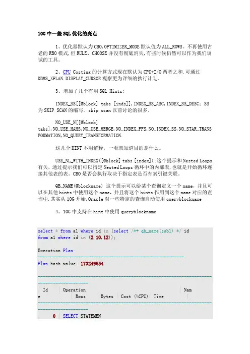
QB_NAME(@blockname) 这个提示可以给某个查询定义一个name,并且可以在其他hints中使用这个name,并且将这个hints作用到这个name对应的查询中.其实从10G开始,Oracle对一些特定的查询自动使用queryblockname4、10G中支持在hint中使用queryblocknameselect*from a1 where id in (select/*+ qb_name(sub1) */ idfrom a1 where id in (2,10,12));Execution Plan----------------------------------------------------------Plan hash value: 173249654-----------------------------------------------------------------------------------------| Id | Operation | Name | Rows | Bytes | Cos t (%CPU)| Time |-----------------------------------------------------------------------------------------|0|SELECT STATEMENT ||2|34|3 (34)|00:00:01||1|TABLE ACCESS BY INDEX ROWID| A1 |1|14|1 (0)|00:00:01||2| NESTED LOOPS ||2|34|3 (34)|00:00:01||3| SORT UNIQUE||2|6|1 (0)|00:00:01||4| INLIST ITERATOR |||||||*5|INDEX RANGE SCAN | IDX_A1_ID |2|6|1 (0)|00:00:01||*6|INDEX RANGE SCAN | IDX_A1_ID |1||0 (0)|00:00:01|--------------------------------------------------------------------------------------------------------select*from a1 where id in (select/*+ qb_name(sub1) full(@sub1 a1) */ idfrom a1 where id in (2,10,12));Plan hash value: 1882950619-----------------------------------------------------------------------------------------| Id | Operation | Name | Rows | Bytes | Cos t (%CPU)| Time |-----------------------------------------------------------------------------------------|0|SELECT STATEMENT ||2|34|17 (6)|00:00:01||1|TABLE ACCESS BY INDEX ROWID| A1 |1|14|1 (0)|00:00:01||2| NESTED LOOPS ||2|34|17 (6)|00:00:01||3| SORT UNIQUE||2|6|15 (0)|00:00:01||*4|TABLE ACCESS FULL| A1 |2|6|15 (0)|00:00:01||*5|INDEX RANGE SCAN | IDX_A1_ID |1||0 (0)|00:00:01|----------------------------------------------------------------------------------------------------修改成错误的queryblocknameselect*from a1 where id in (select/*+ qb_name(sub1) full(@sub2 a1) */ id from a1 where id in (2,10,12));Execution Plan----------------------------------------------------------Plan hash value: 173249654-----------------------------------------------------------------------------------------| Id | Operation | Name | Rows | Bytes | Cos t (%CPU)| Time |-----------------------------------------------------------------------------------------|0|SELECT STATEMENT ||2|34|3 (34)|00:00:01||1|TABLE ACCESS BY INDEX ROWID| A1 |1|14|1 (0)|00:00:01||2| NESTED LOOPS ||2|34|3 (34)|00:00:01||3| SORT UNIQUE||2|6|1 (0)|00:00:01||4| INLIST ITERATOR |||||||*5|INDEX RANGE SCAN | IDX_A1_ID |2|6|1 (0)|00:00:01||*6|INDEX RANGE SCAN | IDX_A1_ID |1||0 (0)|00:00:01|-----------------------------------------------------------------------------------------如果指定的queryblockname未定义,还是保持以前的执行计划,证明queryblockname起作用了.5、新的hints.spread_no_analysis、spread_min_analysis 用于优化analyze查询.具体以后测试下6、10GR2的一些变化.增强了AWR的报告, 提供了专门的ash报告,可以通过新的ashrpt.sql($ORACLE_HOME/rdbms/admin下)脚本产生我们需要的ash报告;提供了类似于statspack获取AWR库中某个sql(通过脚本)的统计信息和执行信息·streams_pool_size现在成为ASSM中的一员·自动调节DB_FILE_MULTIBLOCK_READ_COUNT参数,Oracle会根据数据库的访问自动调节该参数·增加了SQL的优化模式,提供了SQL Tuning Adsivor,SQL Profile等工具.可自动优化sql语句·两个比较重要的视图:v$PROCESS_MEMORY,动态监控每个进程的pga使用,v$sqlstats某种情况下可以替换v$sql视图。

高效利用超级计算技术优化数据分析随着大数据时代的到来,数据分析在各行各业都扮演着至关重要的角色。
而为了更好地实现数据分析,传统的计算机已经远不能满足对数据量和计算复杂度的要求,这时超级计算技术应运而生。
超级计算技术的强大计算能力和高效的并行处理模式,为数据分析提供了更快速、更准确的解决方案。
本文将就高效利用超级计算技术优化数据分析进行探讨。
首先,超级计算技术在数据分析中的优势是不容忽视的。
超级计算机拥有大规模的计算节点,并行处理能力强大,能够同时处理多个任务,大大提升了数据分析的速度和效率。
相对于传统计算机,超级计算机在处理大规模数据时,能够减少计算时间和资源开销,提高数据分析的效果。
其次,利用超级计算技术进行数据分析可以更精确地分析庞大的数据集。
超级计算机的处理能力可使得更复杂的分析任务得以实施。
例如,利用超级计算技术进行模式识别、数据挖掘和深度学习等任务,可以从海量数据中找出隐藏的模式、规律和关联,为企业决策提供有力支持。
通过有效利用超级计算技术,数据分析的结果将更加精准和可靠,为决策者提供基于事实的准确信息,为企业的发展提供有力支撑。
此外,超级计算技术还可以帮助数据分析师更好地应对多样性和复杂性,并在实时场景下快速响应。
大数据分析对数据处理的速度和效率要求较高,而超级计算技术的强大计算能力和高效的并行处理模式,能够快速处理大规模数据集,满足多样化和复杂化数据分析的需求。
在实时场景下,超级计算技术可以提供实时的数据分析结果,及时为决策者提供需要的信息,对企业的运营和发展具有重要意义。
此外,高效利用超级计算技术优化数据分析还需要高质量的算法和模型。
超级计算技术的运用需要配合合适的算法和模型,才能发挥其最大的优势。
数据分析师需要根据具体的问题和数据特点选择合适的算法和模型,在超级计算机上进行优化,并进行实验验证。
通过不断调优和改进,才能实现对大规模数据的高效利用和优化。
最后,高效利用超级计算技术优化数据分析还需要对超级计算技术进行合理的资源调配。


如何让数据库能够实现自我调整,减轻数据库管理员的工作量,是甲骨文公司一直追求的目标。
毕竟其数据库的复杂程度远远超出同类数据库;而且,其数据库的维护成本也比其他数据库要高出不少。
所以,甲骨文公司追求Oracle数据库的自我调整与优化,降低Oracle数据库的维护成本,也是可以理解的。
自我调整SGA与自我调整检查点,虽然是Oracle数据库10G版本中的新增功能,但是,在11G的版本中,才真正发挥到极致,被数据库管理员充分肯定并积极采纳。
下面笔者结合实际的工作经验,带领大家一起看看,这两个新特性,是如何帮助企业降低维护成本,提高数据库的管理效率的。
一、自我调整检查点在以前的文章中,笔者谈到过,Oracle数据库中有存储缓冲区,其包括三部分内容,一种叫做脏缓冲存储区。
这个缓冲存储区中存储的是已经被修改的数据。
一般情况下,这个数据不会马上被写入到数据文件中去。
除非空闲缓冲快用完了,这个数据才会被写入数据文件。
但是,如此的话,也会遇到一个问题,若空闲缓冲区刚用完的时候,其他用户也在频繁的对数据库进行读写操作,在这个繁忙的时刻,再往数据库文件中写入更改后的数据,那么,很明显,会极大的影响数据库的性能。
所以,作为数据库管理员,我们的设想是能否在I/Q操作比较空的时候,就把脏缓冲中的数据写入到数据库中去呢?这若是靠数据库管理员手工管理肯定不现实,我们数据库有这个自动判断的功能。
甲骨文好像听到了我们众多数据库管理员的呼声,在10G版本的数据库中新增了这个功能,并在11G版本中进行了完善,这就是自我调整检查点的自我调整功能。
检查点是将内存中修改的数据与数据库中的数据文件同步的手段。
Oracle数据库定期将检查点之间修改的数据写入数据文件,这种做法的要求之一是需要服务器有足够的可用内存,以提高为即将进行的操作寻找空闲内存的执行性能。
所以,这个检查点的设置,跟很多参数有关,如服务器的内存等等。
虽然在以前的版本中,数据库管理员可以通过设置相关的初始化参数,来指定预期的崩溃恢复时间。

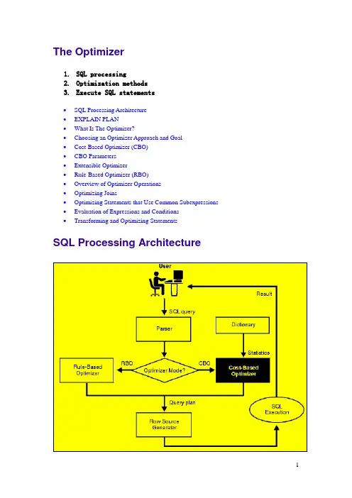
The Optimizer1.SQL processing2.Optimization methods3.Execute SQL statements∙SQL Processing Architecture∙EXPLAIN PLAN∙What Is The Optimizer?∙Choosing an Optimizer Approach and Goal∙Cost-Based Optimizer (CBO)∙CBO Parameters∙Extensible Optimizer∙Rule-Based Optimizer (RBO)∙Overview of Optimizer Operations∙Optimizing Joins∙Optimizing Statements that Use Common Subexpressions ∙Evaluation of Expressions and Conditions∙Transforming and Optimizing StatementsSQL Processing ArchitectureParser∙Syntax analysis: checks SQL statements for correct syntax.∙Semantic analysis: checks if the current database objects and attributes referenced are correct.Optimizer∙rule-based optimizer (RBO)∙cost-based optimizer (CBO)Row Source Generator∙Inputs: optimal plan from the optimizer∙Outputs: execution plan for the SQL statement∙Execution plan: a collection of row sources(a tree)∙Row source: an iterative control structureSQL Execution∙SQL execution: a component that operates on the execution plan ∙Output: the results of the query.What Is The Optimizer?Optimizer: the most efficient way to execute a SQL statementDML statement: SELECT, INSERT, UPDATE, or DELETEInfluence the optimizer: by setting the optimizer approach and goal, by gathering statistics for the CBO, by using hints in SQL statementsExecution PlanAn execution plan includes: an access method for each table and an ordering of the tables (the join order).SELECT ename, job, sal, dnameFROM emp, deptWHERE emp.deptno = dept.deptnoAND NOT EXISTS (SELECT *FROM salgradeWHERE emp.sal BETWEEN losal AND hisal);Steps of Execution Plan∙ A row source : a set of rows returned by a step∙The numbering of the steps: the order for the EXPLAIN PLAN statement ∙Steps indicated by the shaded boxes retrieve data from an object in the database. Such steps are called access paths:o Steps 3 and 6 read all the rows of the emp and salgrade tables, respectively.o Step 5 looks up each deptno value in the pk_deptno index returned by step 3.o Step 4 retrieves the rows whose rowids were returned by step 5 from the dept table.∙Steps indicated by the clear boxes operate on row sources:o Step 2 performs a nested loops operation, accepting row sources from steps 3 and 4, joining each row from step 3 source to its corresponding row in step 4, andreturning the resulting rows to step 1.o Step 1 performs a filter operation. It accepts row sources from steps 2 and 6, eliminates rows from step 2 that have a corresponding row in step 6, and returnsthe remaining rows from step 2 to the user or application issuing the statement. Execution OrderExecution order: form the leaf nodes to root nodes(3,5,4,2,6,1)Choosing an Optimizer Approach and Goal ∙Optimizing for best throughput: result in a full table scan ratherthan an index scan, or a sort-merge join rather than a nested loops join.∙Optimizing for best response time:,results in an index scan or a nested loops join.∙For applications performed in batch, such as Oracle Reports applications, optimize for best throughput.∙For interactive applications, such as Oracle Forms applications or SQL*Plus queries, optimize for best response time.∙For queries hat use ROWNUM to limit the number of rows, optimize for best response time.OPTIMIZER_MODE Initialization ParameterCHOOSE contains statistics for at least one of the accessed tables:a cost-based approach and best throughputcontains no statistics for any of the accessed tables: arule-based approach(default value).ALL_ROWS a cost-based approach and best throughput (minimum resource use to complete the entire statement).FIRST_ROWS a cost-based approach and best response time (minimum resource use to return the first row of the set).RULE a rule-based approachinternal information (such as the number of data blocks allocated to these tables)Statistics in the Data Dictionary●Statistics: columns, tables, clusters, indexes, and partitions(CBO).●collect exact or estimated statistics: DBMS_STATS package, theANALYZE statement, or the COMPUTE STATISTICS clause OPTIMIZER_GOAL Parameter of the ALTER SESSION Statement ●OPTIMIZER_GOAL parameter: can override OPTIMIZER_MODE●Affect: the optimization of SQL statements issued by storedprocedures and functions called during the session●does not affect: the optimization of recursive SQL statements thatOracle issues during the session.CHOOSE contains statistics for at least one of the accessed tables:a cost-based approach and best throughputcontains no statistics for any of the accessed tables: arule-based approachALL_ROWS a cost-based approach and best throughput (minimum resource use to complete the entire statement).FIRST_ROWS a cost-based approach and best response time (minimum resource use to return the first row of the result set).RULE a rule-based approachChanging the Goal with HintsHint( FIRST_ROWS, ALL_ROWS, CHOOSE, or RULE): override OPTIMIZER_MODE and OPTIMIZER_GOAL.ALTER SESSION SET OPTIMIZER_MODE = FIRST_ROWS;Cost-Based Optimizer (CBO)In general, you should always use the cost-based approach. The rule-based approach is available for the benefit of existing applications.1.The optimizer generates a set of potential plans for the SQL statementbased on its available access paths and hints.2.The optimizer estimates the cost of each plan based on statistics in thedata dictionary for the data distribution and storage characteristics of the tables, indexes, and partitions accessed by the statement.3.The optimizer compares the costs of the plans and chooses the one withthe smallest cost.To maintain the effectiveness of the CBO, you must gather statistics and keep them current.Architecture of the CBOQuery Transformer●Input: a parsed query(represented by a set of query blocks)●Main objective: determine if it is advantageous to change the formof the query, so that it enables generation of a better query plan ●Three query transformation techniques: view merging, subqueryunnesting, and query rewrite using materialized views(combination) Estimator●Three different types of measures: selectivity, cardinality(基数),and cost.●The end goal of the estimator: estimate the overall cost of a givenplan.●Selectivity: a fraction of rows from a row set, the selectivity ofa predicate indicates how many rows from a row set will pass thepredicate test.●Cardinality: the number of rows in a row set.●Cost: units of work or resource used. The CBO uses disk I/O as a unitof work.Plan Generator●Main function: try out different possible plans for a given query andpick the one that has the lowest cost.Features that Require the CBO∙Partitioned tables∙Index-organized tables∙Reverse key indexes∙Function-based indexes∙SAMPLE clauses in a SELECT statement∙Parallel execution and parallel DML∙Star transformations∙Star joins∙Extensible optimizer∙Query rewrite (materialized views)∙Progress meter∙Hash joins∙Bitmap indexes∙Partition views (release 7.3)Using the CBOTo use the CBO for a statement, collect statistics and enable the CBO: ∙Make sure that the OPTIMIZER_MODE initialization parameter is set to itsdefault value of CHOOSE.∙To enable the CBO for your session only, issue an ALTER SESSION SET OPTIMIZER_MODE statement with the ALL_ROWS or FIRST_ROWS clause.∙To enable the CBO for an individual SQL statement, use any hint other than RULE.Access Paths for the CBO● A full table scan: retrieves rows from a table. can be performedvery efficiently using multiblock reads.● A sample table scan: retrieves a random sample of data from a tablewhen the statement's FROM clause includes the SAMPLE clause or the SAMPLE BLOCK clause.[SELECT * FROM emp SAMPLE BLOCK (1); (1%)]● A table access by rowed: retrieves rows from a table. Locating arow by its rowid is the fastest way for Oracle to find a single row.● A cluster scan: retrieves rows that have the same cluster key value.In an indexed cluster, all rows with the same cluster key value are stored in the same data blocks.● A hash scan: locate rows in a hash cluster based on a hash value.In a hash cluster, all rows with the same hash value are stored in the same data blocks.●An index scan: retrieves data from an index based on the value ofone or more columns of the index.(types: Unique/Range/Full/Fastfull/Index join/Bitmap)How the CBO Chooses an Access Path∙The available access paths for the statement.∙The estimated cost of executing the statement using each access path or combination of paths.Extensible OptimizerIt allows the authors of user-defined functions and domain indexes to control the three main components that the CBO uses to select an execution plan: statistics, selectivity, and cost evaluation.Overview of Optimizer Operations●the types of SQL statements that can be optimized●the operations performed by the optimizerTypes of SQL StatementsSimple statement An INSERT, UPDATE, DELETE, or SELECT statement thatinvolves only a single table.Simple query Another name for a SELECT statement.Join A query that selects data from more than one table. Equijoin A join condition containing an equality operator. Non-equijoin A join condition containing something other than anequality operator.Outer join A join condition using the outer join operator (+) withone or more columns of one of the tables.Cartesian product A join with no join condition results in a Cartesianproduct, or a cross product.Complex statement An INSERT, UPDATE, DELETE, or SELECT statement thatcontains a subquery.Compound query A query that uses set operators (UNION, UNION ALL,INTERSECT, or MINUS) to combine two or more simple orcomplex statements.Statement accessing views Simple, join, complex, or compound statement that accesses one or more views as well as tables.Distributed statement A statement that accesses data on two or more distinct nodes of a distributed database.Optimizer Operations1 Evaluation of expressions and conditions2 Statement transformation3 View merging4 Choice of optimizer approaches5 Choice of access paths6 Choice of join orders7 Choice of join operationsOptimizing Joins●how the optimizer executes SQL statements that contain joins,anti-joins, and semi-joins●how the optimizer can use bitmap indexes to execute star queries,which join a fact table to multiple dimension tablesOptimizing Join StatementsAccess Paths As for simple statements, the optimizer must choose an access path to retrieve data from each table in the join statement.Join Operations To join each pair of row sources, Oracle must perform one of these operations:∙Nested Loops (NL) Join∙Sort-Merge Join∙Hash Join (not available with the RBO)∙Cluster JoinJoin Order Oracle joins two of the tables, and then joins the resulting row source to the next table.Join OperationsNested Loops (NL) Join1.The optimizer chooses one of the tables as the outer table, or the drivingtable. The other table is called the inner table.2.For each row in the outer table, Oracle finds all rows in the inner tablethat satisfy the join condition.3.Oracle combines the data in each pair of rows that satisfy the joincondition and returns the resulting rows.Sort-Merge Join1.Oracle sorts each row source to be joined if they have not been sortedalready by a previous operation. The rows are sorted on the values of the columns used in the join condition.2.Oracle merges the two sources so that each pair of rows, one from eachsource, that contain matching values for the columns used in the join condition are combined and returned as the resulting row source.Hash Join1.Oracle performs a full table scan on each of the tables and splits each intoas many partitions as possible based on the available memory.2.Oracle builds a hash table from one of the partitions (if possible, Oracleselects a partition that fits into available memory). Oracle then uses the corresponding partition in the other table to probe the hash table. All partition pairs that do not fit into memory are placed onto disk.3.For each pair of partitions (one from each table), Oracle uses the smallerone to build a hash table and the larger one to probe the hash table. Cluster JoinOracle can perform a cluster join only for an equijoin that equates the cluster key columns of two tables in the same cluster.Evaluation of Expressions and ConditionsHow the optimizer evaluates expressions and conditions that contain the following:∙Constants∙LIKE Operator∙IN Operator∙ANY or SOME Operator∙ALL Operator∙BETWEEN Operator∙NOT Operator∙Transitivity(传递性)∙DETERMINISTIC FunctionsConstantsComputation of constants is performed only once, when the statement is optimized, rather than each time the statement is executed.sal > 24000/12sal > 2000sal*12 > 24000The optimizer does not simplify expressions across comparison operators.LIKE OperatorThe optimizer simplifies conditions that use the LIKE comparison operator to compare an expression with no wildcard characters into an equivalent condition that uses an equality operator instead.ename LIKE 'SMITH'ename = 'SMITH'The optimizer can simplify these expressions only when the comparison involves variable-length datatypes.IN OperatorThe optimizer expands a condition that uses the IN comparison operator to an equivalent condition that uses equality comparison operators and OR logical operators.ename IN ('SMITH', 'KING', 'JONES')ename = 'SMITH' OR ename = 'KING' OR ename = 'JONES'ANY or SOME OperatorThe optimizer expands a condition that uses the ANY or SOME comparison operator followed by a parenthesized list of values into an equivalent condition that uses equality comparison operators and OR logical operators.sal > ANY (:first_sal, :second_sal)sal > :first_sal OR sal > :second_salThe optimizer transforms a condition that uses the ANY or SOME operator followed by a subquery into a condition containing the EXISTS operator and a correlated subquery.x > ANY (SELECT sal FROM emp WHERE job = 'ANALYST')EXISTS (SELECT sal FROM emp WHERE job = 'ANALYST' AND x > sal)ALL OperatorThe optimizer expands a condition that uses the ALL comparison operator followed by a parenthesized list of values into an equivalent condition that uses equality comparison operators and AND logical operators.sal > ALL (:first_sal, :second_sal)sal > :first_sal AND sal > :second_salThe optimizer transforms a condition that uses the ALL comparison operator followed by a subquery into an equivalent condition that uses the ANY comparison operator and a complementary comparison operator.x > ALL (SELECT sal FROM emp WHERE deptno = 10)NOT (x <= ANY (SELECT sal FROM emp WHERE deptno = 10) )The optimizer then transforms the second query into the following query using the rule for transforming conditions with the ANY comparison operator followed by a correlated subquery:NOT EXISTS (SELECT sal FROM emp WHERE deptno = 10 AND x <= sal)BETWEEN OperatorThe optimizer always replaces a condition that uses the BETWEEN comparison operator with an equivalent condition that uses the >= and <= comparison operators.sal BETWEEN 2000 AND 3000sal >= 2000 AND sal <= 3000NOT OperatorThe optimizer simplifies a condition to eliminate the NOT logical operator. The simplification involves removing the NOT logical operator and replacing a comparison operator with its opposite comparison operator.NOT deptno = (SELECT deptno FROM emp WHERE ename = 'TAYLOR')deptno <> (SELECT deptno FROM emp WHERE ename = 'TAYLOR')NOT (sal < 1000 OR comm IS NULL)NOT sal < 1000 AND comm IS NOT NULLsal >= 1000 AND comm IS NOT NULLTransitivityIf two conditions in the WHERE clause involve a common column, then the optimizer can sometimes infer a third condition using the transitivity principle.WHERE column1 comp_oper constantAND column1 = column2In this case, the optimizer infers the condition:column2 comp_oper constantSELECT * FROM emp, deptWHERE emp.deptno = 20AND emp.deptno = dept.deptno;Using transitivity, the optimizer infers this condition:dept.deptno = 20If an index exists on the dept.deptno column, then this condition makes available access paths using that index.DETERMINISTIC FunctionsIn some cases, the optimizer can use a previously calculated value, rather than executing a user-written function.Transforming and Optimizing Statements ∙Transforming ORs into Compound Queries∙Transforming Complex Statements into Join Statements∙Optimizing Statements That Access Views∙Optimizing Compound Queries∙Optimizing Distributed StatementsTransforming ORs into Compound Queries∙If each condition individually makes an index access path available, then the optimizer can make the transformation.∙If any condition requires a full table scan because it does not make an index available, then the optimizer does not transform the statement∙For statements that use the CBO, the optimizer may use statistics todetermine whether to make the transformation.∙The CBO does not use the OR transformation for IN-lists or OR s on the same column; instead, it uses the INLIST iterator operator.SELECT * FROM emp WHERE job = 'CLERK' OR deptno = 10;If there are indexes on both the job and deptno columns:SELECT * FROM emp WHERE job = 'CLERK'UNION ALLSELECT * FROM emp WHERE deptno = 10 AND job <> 'CLERK';SELECT * FROM emp WHERE ename = 'SMITH' OR sal > comm;If there is an index on the ename column only:SELECT * FROM emp WHERE ename = 'SMITH'UNION ALLSELECT * FROM emp WHERE sal > comm;Transforming Complex Statements into Join Statements ∙Transform the complex statement into an equivalent join statement, andthen optimize the join statement.∙Optimize the complex statement as it is.SELECT * FROM accountsWHERE custno IN (SELECT custno FROM customers);If the custno column of the customers table is a primary key or has a UNIQUE constraint:SELECT accounts.*FROM accounts, customersWHERE accounts.custno = customers.custno;SELECT * FROM accountsWHERE accounts.balance > (SELECT AVG(balance) FROM accounts);No join statement can perform the function of this statement, so the optimizer does not transform the statement.Optimizing Statements That Access Views(help for yourself) Optimizing Compound Queries●chooses an execution plan for each query of its component queries ●combines the resulting row sources with the union, intersection, orminus operationSELECT part FROM orders1UNION ALLSELECT part FROM orders2;Optimizing Distributed StatementsIn much the same way for statements that access only local data: ∙If all the tables accessed by a SQL statement are collocated on the same remote database, then Oracle sends the SQL statement to that remote database.∙If a SQL statement accesses tables that are located on different databases, then Oracle decomposes the statement into individual fragments, each of which accesses tables on a single database. Oracle then sends each fragment to the database that it accesses.。
Oracle优化器(Optimizer)是Oracle在执行SQL之前分析语句的工具。
Oracle的优化器有两种优化方式:基于规则的优化方式:Rule-Based Optimization(RBO)优化器在分析SQL语句时,所遵循的是Oracle内部预定的一些规则。
比如我们常见的,当一个where子句中的一列有索引时去走索引。
基于成本或者统计信息的优化方式(Cost-Based Optimization:CBO)CBO是在ORACLE7 引入,但到ORACLE8i 中才成熟。
ORACLE 已经声明在ORACLE9i之后的版本中,RBO将不再支持。
它是看语句的代价(Cost),这里的代价主要指Cpu和内存。
CPU Costing的计算方式现在默认为CPU+I/O两者之和.可通过DBMS_XPLAN.DISPLAY_CURSOR观察更为详细的执行计划。
优化器在判断是否用这种方式时,主要参照的是表及索引的统计信息。
统计信息给出表的大小、有少行、每行的长度等信息。
这些统计信息起初在库内是没有的,是做analyze后才出现的,很多的时侯过期统计信息会令优化器做出一个错误的执行计划,因些应及时更新这些信息。
按理,CBO应该自动收集,实际却不然,有时候在CBO情况下,还必须定期对大表进行分析。
Oracle优化器的优化模式:1) CHOOSE仅在9i及之前版本中被支持,10g已经废除。
8i及9i中为默认值。
这个值表示SQL语句既可以使用RBO优化器也可以使用CBO优化器,而决定该SQL到底使用哪个优化器的唯一因素是,所访问的对象是否存在统计信息。
如果所访问的全部对象都存在统计信息,则使用CBO 优化器优化SQL;如果只有部分对象存在统计信息,也仍然使用CBO优化器优化SQL,优化器会为不存在统计信息对象依据一些内在信息(如分配给该对象的数据块)来生成统计信息,只是这样生成的统计信息可能不准确,而导致产生不理想的执行计划;如果全部对象都无统计信息,则使用RBO来优化该SQL 语句。
lstm 模型及优化算法soa python -回复LSTM模型及优化算法SOA(State-of-the-art)PYTHON引言:LSTM(长短期记忆,Long Short-Term Memory)是一种特殊的循环神经网络(RNN)模型,适用于序列数据预测和文本生成等任务。
同时,优化算法SOA帮助我们提高LSTM模型的性能,并取得更好的预测结果。
本文将一步一步介绍LSTM模型以及优化算法SOA在Python中的应用。
第一部分:LSTM模型介绍1. 什么是LSTM模型?LSTM是一种具有“记忆”机制的RNN模型。
与传统RNN相比,LSTM 通过内部的门控单元,可以更好地处理长期依赖关系,避免梯度消失或爆炸的问题。
2. LSTM模型的结构LSTM模型由输入门(input gate)、遗忘门(forget gate)、输出门(output gate)和细胞状态(cell state)组成。
这些门控单元决定了信息的传递和保持,使得模型能够有效地学习和记忆序列信息。
3. LSTM模型的优势LSTM模型相比于传统RNN模型具有以下优势:- 能够处理长期依赖关系- 缓解梯度消失或梯度爆炸问题- 具备较好的记忆和预测能力第二部分:优化算法SOA介绍1. 什么是优化算法SOA?SOA(State-of-the-art)是指某个领域当前最先进和最优秀的算法。
在神经网络训练中,SOA通常是指最新的梯度优化算法,如Adam、RMSProp等。
2. Adam优化算法Adam算法结合了自适应矩估计(adaptive moment estimation)和Root Mean Square Propagation(RMSProp)算法的优点,对梯度进行适应性调整。
它有效地解决了梯度消失或爆炸的问题,并提高了模型的训练速度和收敛性。
3. 如何在Python中使用Adam算法优化LSTM模型?在Python中使用Adam算法优化LSTM模型可以通过以下步骤实现:- 导入相应的库和模块:如numpy、keras等- 构建LSTM模型:使用keras搭建LSTM模型,并设置合适的超参数和模型结构- 编译模型:使用Adam算法作为优化器,并选择适当的损失函数和评估指标- 模型训练:使用训练数据对模型进行训练,并监控训练过程中的损失和性能指标- 模型评估和预测:使用测试数据对模型进行评估,并对新数据进行预测和生成第三部分:示例代码和讨论以下是使用Python实现LSTM模型并使用Adam算法进行优化的示例代码:pythonimport numpy as npfrom keras.models import Sequentialfrom yers import LSTM, Densefrom keras.optimizers import Adam# 生成训练数据X_train = ...Y_train = ...# 构建LSTM模型model = Sequential()model.add(LSTM(units=64, input_shape=(timesteps, features))) model.add(Dense(units=32, activation='relu'))model.add(Dense(units=num_classes, activation='softmax'))# 编译模型modelpile(optimizer=Adam(), loss='categorical_crossentropy', metrics=['accuracy'])# 模型训练model.fit(X_train, Y_train, epochs=10, batch_size=32)# 模型评估和预测X_test = ...Y_test = ...loss, accuracy = model.evaluate(X_test, Y_test)predictions = model.predict(X_test)以上示例代码中,我们使用了keras库来构建LSTM模型,并使用Adam算法作为优化器。

数据实验室:让数据获得真正的价值Babar Jan-Haleem【摘要】根据领先的独立研究机构Forrester的论述,企业数据仓库正通过扩展性、性能和创新不断发展,已超越了传统的数据存储和传递。
面对巨量的数据,许多公司开始采用现代化的开采工具,并从这种新形式的经济资源中获取价值。
事实上,一些有前瞻性的组织在多年前甚至几十年前就开始利用大数据来获取洞察。
这是一个不断演变的、并由越来越大的数据量驱动的大数据之旅。
【期刊名称】《中国建设信息化》【年(卷),期】2016(000)018【总页数】2页(P26-27)【关键词】企业数据仓库 Forrester 甲骨文公司信用卡支付分布式存储主要流程现金支付用户体验核心商业业务线【作者】Babar Jan-Haleem【作者单位】甲骨文亚太区;【正文语种】中文【中图分类】TP392面对巨量的数据,许多公司开始采用现代化的开采工具,并从这种新形式的经济资源中获取价值。
事实上,一些有前瞻性的组织在多年前甚至几十年前就开始利用大数据来获取洞察。
这是一个不断演变的、并由越来越大的数据量驱动的大数据之旅。
而数据的流速和变化速度也在加快。
由业务交易所产生的高度结构化的、精确的、并经过验证的数据通常被存放在更加常见的数据集市和数据仓库中,但企业同时也从企业外部,由传感器、人或流程产生数据或收集数据。
依靠数据和网络提取核心商业价值获得巨大成功的企业案例比比皆是,如Airbnb和优步,他们并不拥有有形资产。
不久前,搭乘出租车意味着你需要在大街上挥手拦下出租车,告诉司机你的目的地,并以现金支付车费,整个过程中没有任何数据的参与。
而今天,你打开你的手机叫车软件,实时跟踪GPS定位的路线,最后用信用卡支付出租车费,再通过社交媒体平台给司机写下评分,同时司机也可对你的这次乘车写下评论。
单是这样的一次乘车就创建了四种类型的数据。
这些原始的、非结构化的数据大量驻留在“数据水库”或“数据湖中”,如何从这些“数据水库”中提取价值,成为了以大数据为主角的故事中很重要的一部分。

oraclesqloptimizeOracle sql 性能优化调整1. 选用适合的ORACLE优化器ORACLE的优化器共有3种:a. RULE (基于规则)b. COST (基于成本)c. CHOOSE (选择性)设置缺省的优化器,可以通过对init.ora文件中OPTIMIZER_MODE参数的各种声明,如RULE,COST,CHOOSE,ALL_ROWS,FIRST_ROWS . 你当然也在SQL句级或是会话(session)级对其进行覆盖.为了使用基于成本的优化器(CBO, Cost-Based Optimizer) , 你必须经常运行analyze 命令,以增加数据库中的对象统计信息(object statistics)的准确性.如果数据库的优化器模式设置为选择性(CHOOSE),那么实际的优化器模式将和是否运行过analyze命令有关. 如果table已经被analyze过, 优化器模式将自动成为CBO , 反之,数据库将采用RULE形式的优化器.在缺省情况下,ORACLE采用CHOOSE优化器, 为了避免那些不必要的全表扫描(full table scan) , 你必须尽量避免使用CHOOSE优化器,而直接采用基于规则或者基于成本的优化器.2.访问Table的方式ORACLE 采用两种访问表中记录的方式:a.全表扫描全表扫描就是顺序地访问表中每条记录. ORACLE采用一次读入多个数据块(database block)的方式优化全表扫描.b.通过ROWID访问表你可以采用基于ROWID的访问方式情况,提高访问表的效率, , ROWID包含了表中记录的物理位置信息..ORACLE采用索引(INDEX)实现了数据和存放数据的物理位置(ROWID)之间的联系. 通常索引提供了快速访问ROWID的方法,因此那些基于索引列的查询就可以得到性能上的提高.3.共享SQL语句为了不重复解析相同的SQL语句,在第一次解析之后, ORACLE将SQL语句存放在内存中.这块位于系统全局区域SGA(system global area)的共享池(shared buffer pool)中的内存可以被所有的数据库用户共享.因此,当你执行一个SQL语句(有时被称为一个游标)时,如果它和之前的执行过的语句完全相同, ORACLE就能很快获得已经被解析的语句以及最好的执行路径. ORACLE的这个功能大大地提高了SQL的执行性能并节省了内存的使用.可惜的是ORACLE只对简单的表提供高速缓冲(cache buffering) ,这个功能并不适用于多表连接查询.数据库管理员必须在init.ora中为这个区域设置合适的参数,当这个内存区域越大,就可以保留更多的语句,当然被共享的可能性也就越大了.当你向ORACLE 提交一个SQL语句,ORACLE会首先在这块内存中查找相同的语句.这里需要注明的是,ORACLE对两者采取的是一种严格匹配,要达成共享,SQL语句必须完全相同(包括空格,换行等).共享的语句必须满足三个条件:A.字符级的比较:当前被执行的语句和共享池中的语句必须完全相同.例如:SELECT * FROM EMP;和下列每一个都不同SELECT * from EMP;Select * From Emp;SELECT * FROM EMP;B.两个语句所指的对象必须完全相同:例如:用户对象名如何访问Jack sal_limit private synonymWork_city public synonymPlant_detail public synonymJill sal_limit private synonymWork_city public synonymPlant_detail table owner考虑一下下列SQL语句能否在这两个用户之间共享.C.两个SQL语句中必须使用相同的名字的绑定变量(bind variables)例如:第一组的两个SQL语句是相同的(可以共享),而第二组中的两个语句是不同的(即使在运行时,赋于不同的绑定变量相同的值)a.select pin , name from people where pin = :blk1.pin;select pin , name from people where pin = :blk1.pin;b.select pin , name from people where pin = :blk1.ot_ind;select pin , name from people where pin = :blk1.ov_ind;4. 选择最有效率的表名顺序(只在基于规则的优化器中有效)ORACLE的解析器按照从右到左的顺序处理FROM子句中的表名,因此FROM子句中写在最后的表(基础表driving table)将被最先处理.在FROM子句中包含多个表的情况下,你必须选择记录条数最少的表作为基础表.当ORACLE处理多个表时, 会运用排序及合并的方式连接它们.首先,扫描第一个表(FROM子句中最后的那个表)并对记录进行派序,然后扫描第二个表(FROM子句中最后第二个表),最后将所有从第二个表中检索出的记录与第一个表中合适记录进行合并.例如: 表TAB1 16,384 条记录表TAB2 1 条记录选择TAB2作为基础表(最好的方法)select count(*) from tab1,tab2 执行时间0.96秒选择TAB2作为基础表(不佳的方法)select count(*) from tab2,tab1 执行时间26.09秒如果有3个以上的表连接查询, 那就需要选择交叉表(intersection table)作为基础表, 交叉表是指那个被其他表所引用的表.例如: EMP表描述了LOCA TION表和CATEGORY表的交集.SELECT *FROM LOCATION L ,CATEGORY C,EMP EWHERE E.EMP_NO BETWEEN 1000 AND 2000AND E.CAT_NO = C.CAT_NOAND E.LOCN = L.LOCN将比下列SQL更有效率SELECT *FROM EMP E ,LOCATION L ,CATEGORY CWHERE E.CAT_NO = C.CA T_NOAND E.LOCN = L.LOCNAND E.EMP_NO BETWEEN 1000 AND 20005.WHERE子句中的连接顺序.ORACLE采用自下而上的顺序解析WHERE子句,根据这个原理,表之间的连接必须写在其他WHERE条件之前, 那些可以过滤掉最大数量记录的条件必须写在WHERE子句的末尾.例如:(低效,执行时间156.3秒)SELECT …FROM EMP EWHERE SAL > 50000AND JOB = ‘MANAGER’AND 25 < (SELECT COUNT(*) FROM EMPWHERE MGR=E.EMPNO);(高效,执行时间10.6秒)SELECT …FROM EMP EWHERE 25 < (SELECT COUNT(*) FROM EMPWHERE MGR=E.EMPNO)AND SAL > 50000AND JOB = ‘MANAGER’;6.SELECT子句中避免使用‘ * ‘当你想在SELECT子句中列出所有的COLUMN时,使用动态SQL列引用‘*’ 是一个方便的方法.不幸的是,这是一个非常低效的方法. 实际上,ORACLE在解析的过程中, 会将’*’ 依次转换成所有的列名, 这个工作是通过查询数据字典完成的, 这意味着将耗费更多的时间.7.减少访问数据库的次数当执行每条SQL语句时, ORACLE在内部执行了许多工作: 解析SQL语句, 估算索引的利用率, 绑定变量, 读数据块等等. 由此可见, 减少访问数据库的次数, 就能实际上减少ORACLE的工作量.例如,以下有三种方法可以检索出雇员号等于0342或0291的职员.方法1 (最低效)SELECT EMP_NAME , SALARY , GRADEFROM EMPWHERE EMP_NO = 342;SELECT EMP_NAME , SALARY , GRADEFROM EMPWHERE EMP_NO = 291;方法2 (次低效)DECLARECURSOR C1 (E_NO NUMBER) ISSELECT EMP_NAME,SALARY,GRADEFROM EMPWHERE EMP_NO = E_NO;BEGINOPEN C1(342);SELECT C1 INTO …,…,…;FETCH C1 INTO …,..,.. ;OPEN C1(291);FETCH C1 INTO …,..,.. ;CLOSE C1;END;方法3 (高效)SELECT A.EMP_NAME , A.SALARY , A.GRADE,B.EMP_NAME , B.SALARY , B.GRADEFROM EMP A,EMP BWHERE A.EMP_NO = 342AND B.EMP_NO = 291;注意:在SQL*Plus , SQL*Forms和Pro*C中重新设置ARRAYSIZE参数, 可以增加每次数据库访问的检索数据量,建议值为200.8.使用DECODE函数来减少处理时间使用DECODE函数可以避免重复扫描相同记录或重复连接相同的表.例如:SELECT COUNT(*),SUM(SAL)FROM EMPWHERE DEPT_NO = 0020AND ENAME LIKE‘SMITH%’;SELECT COUNT(*),SUM(SAL)FROM EMPWHERE DEPT_NO = 0030AND ENAME LIKE‘SMITH%’;你可以用DECODE函数高效地得到相同结果SELECT COUNT(DECODE(DEPT_NO,0020,’X’,NULL)) D0020_COUNT,COUNT(DECODE(DEPT_NO,0030,’X’,NULL)) D0030_COUNT,SUM(DECODE(DEPT_NO,0020,SAL,NULL)) D0020_SAL,SUM(DECODE(DEPT_NO,0030,SAL,NULL)) D0030_SALFROM EMP WHERE ENAME LIKE ‘SMITH%’;类似的,DECODE函数也可以运用于GROUP BY 和ORDER BY子句中.9.整合简单,无关联的数据库访问如果你有几个简单的数据库查询语句,你可以把它们整合到一个查询中(即使它们之间没有关系)例如:SELECT NAMEFROM EMPWHERE EMP_NO = 1234;SELECT NAMEFROM DPTWHERE DPT_NO = 10 ;SELECT NAMEFROM CATWHERE CAT_TYPE = ‘RD’;上面的3个查询可以被合并成一个:SELECT , , FROM CAT C , DPT D , EMP E,DUAL XWHERE NVL(‘X’,X.DUMMY) = NVL(‘X’,E.ROWID(+))AND NVL(‘X’,X.DUMMY) = NVL(‘X’,D.ROWID(+))AND NVL(‘X’,X.DUMMY) = NVL(‘X’,C.ROWID(+))AND E.EMP_NO(+) = 1234AND D.DEPT_NO(+) = 10AND C.CAT_TYPE(+) = ‘RD’;(译者按: 虽然采取这种方法,效率得到提高,但是程序的可读性大大降低,所以读者还是要权衡之间的利弊)10.删除重复记录最高效的删除重复记录方法( 因为使用了ROWID)DELETE FROM EMP EWHERE E.ROWID > (SELECT MIN(X.ROWID)FROM EMP XWHERE X.EMP_NO = E.EMP_NO);11.用TRUNCATE替代DELETE当删除表中的记录时,在通常情况下, 回滚段(rollback segments ) 用来存放可以被恢复的信息. 如果你没有COMMIT事务,ORACLE会将数据恢复到删除之前的状态(准确地说是恢复到执行删除命令之前的状况)而当运用TRUNCATE时, 回滚段不再存放任何可被恢复的信息.当命令运行后,数据不能被恢复.因此很少的资源被调用,执行时间也会很短.(译者按: TRUNCATE只在删除全表适用,TRUNCATE是DDL不是DML)12.尽量多使用COMMIT只要有可能,在程序中尽量多使用COMMIT, 这样程序的性能得到提高,需求也会因为COMMIT所释放的资源而减少:COMMIT所释放的资源:a.回滚段上用于恢复数据的信息.b.被程序语句获得的锁c.redo log buffer 中的空间d.ORACLE为管理上述3种资源中的内部花费(译者按: 在使用COMMIT时必须要注意到事务的完整性,现实中效率和事务完整性往往是鱼和熊掌不可得兼)13.计算记录条数和一般的观点相反, count(*) 比count(1)稍快, 当然如果可以通过索引检索,对索引列的计数仍旧是最快的. 例如COUNT(EMPNO)(译者按: 在CSDN论坛中,曾经对此有过相当热烈的讨论, 作者的观点并不十分准确,通过实际的测试,上述三种方法并没有显著的性能差别)14.用Where子句替换HA VING子句避免使用HA VING子句, HA VING 只会在检索出所有记录之后才对结果集进行过滤. 这个处理需要排序,总计等操作. 如果能通过WHERE子句限制记录的数目,那就能减少这方面的开销.例如:低效:SELECT REGION,A VG(LOG_SIZE)FROM LOCATIONGROUP BY REGIONHA VING REGION REGION != ‘SYDNEY’AND REGION != ‘PERTH’高效SELECT REGION,A VG(LOG_SIZE)FROM LOCATIONW HERE REGION REGION != ‘SYDNEY’AND REGION != ‘PERTH’GROUP BY REGION(译者按: HAVING 中的条件一般用于对一些集合函数的比较,如COUNT() 等等. 除此而外,一般的条件应该写在WHERE子句中)15.减少对表的查询在含有子查询的SQL语句中,要特别注意减少对表的查询.例如:低效SELECT TAB_NAMEFROM TABLESWHERE TAB_NAME = ( SELECT TAB_NAMEFROM TAB_COLUMNS。
Quest®SQL Optimizer for Oracle8.8《用户指南》©2013Quest Software,Inc.保留所有权利。
本指南包含受版权保护的专利信息。
本指南中描述的软件根据软件许可证或保密协议提供。
只能根据适用协议的条款使用或复制此软件。
未经Quest Software,Inc.书面许可,禁止以任何形式或通过任何方式,无论电子或机械方式(包括出于任何目的的影印和记录,购买者个人使用除外)复制或传输本指南任何部分。
本文的信息涉及Quest产品。
本文或Quest产品的销售未以禁止翻供或其他方式对任何知识产权授予明示或暗示的许可证。
除了本产品许可证协议规定的Quest条款和条件,Quest 不会承担任何责任并拒绝承认与其产品相关的任何明示、暗示或法定保证,包括但不限于适销性、适合某一目的或不侵权的暗示保证。
在任何情况下,Quest不会对使用本文档或未能使用本文档而产生的任何直接损害、间接损害、后果损害、惩罚性损害、特殊损害或附带损害(包括但不限于对于利润损失、业务中断或信息损失的损害)负责。
Quest不会对本文的准确性或完整性发表任何声明或保证,并且保留在不发出通知的情况下随时更改规范和产品描述的权利。
Quest不会承诺更新本文的信息。
如果您对本材料的潜在使用有任何疑问,请联系:Quest Software World HeadquartersLEGAL Dept5Polaris WayAliso Viejo,CA92656电子邮件:legal@请访问我们的网站()了解地区办事处和国际办事处的信息。
专利SQL Optimizer for Oracle包含正在申请专利的技术。
商标Quest、Quest Software、Quest Software标识、Simplicity at Work、Benchmark Factory、Foglight、LeccoTech、Quest vWorkspace、SQLab、Toad及T.O.A.D是Quest Software,Inc.的商标和注册商标。
甲骨文:与开源数据库不是竞争而是共存张鹏【期刊名称】《通信世界》【年(卷),期】2015(000)021【总页数】1页(P39)【作者】张鹏【作者单位】【正文语种】中文甲骨文不断探索云中迁移的解决方案,如何更加快速和透明,只需要写一次应用就可以完成迁移,为此甲骨文不断提升自身在内存技术、多租户、集成系统等方面的能力。
甲骨文集团副总裁及亚太区技术产品事业部总经理 .....孔睿士(Chris Chelliah)甲骨文全球副总裁及亚洲研究开发中心总经 ...........理博斯佳(Pascal Sero)甲骨文公司副总裁及中国区技术产品事业部总经理 .....................吴承扬作为全球最大的软件企业之一,甲骨文公司的发展历程见证了IT行业的兴衰与成长。
据数据显示,在全球财富500强的企业中,有98%的客户采用了Oracle数据库,在全球前10大云服务提供商中,有9家采用Oracle数据库。
据悉,在甲骨文最近一期的财年结束后,该公司将成为全球云服务排名第一的公司。
2015年恰是甲骨文公司成立38周年,其中国区成立28周年,在7月23日召开的甲骨文数据大会上,来自国内政府、学校以及各行业领域的客户代表齐聚一堂,在见证甲骨文38年发展历程的同时,也为IT行业未来的发展与演进共商大计。
《通信世界》记者也对三位甲骨文的高层领导进行了专访。
Q:围绕数据管理,在未来甲骨文有何发展规划?孔睿士:数据管理可以说既是甲骨文的背景,也是我们的历史,在过去几十年里,甲骨文始终围绕该领域向客户提供解决方案以应对数据爆炸性的增长。
时下,业界很多新技术不断涌现,从关系型数据库、分布式系统、服务器、互联网计算乃至云计算,甲骨文的目标是让客户和合作伙伴更快地适应并采纳这些新技术,将风险和成本降至最低,为此甲骨文不断为平台的创新而进行投资。
甲骨文不断探索云中迁移的解决方案,如何更加快速和透明,只需要写一次应用就可以完成迁移,为此甲骨文不断提升自身在内存技术、多租户、集成系统等方面的能力,希望更好地帮助客户进行本地部署以及云中部署。
ORACLE数据库系统优化
郭利松;王敏
【期刊名称】《光电技术应用》
【年(卷),期】2003(018)003
【摘要】ORACLE数据库系统的参数中有很多存在着调优问题,尤其对一些主要参数,若配置合理将会大大提高系统的运行效率.分析讨论了就系统安装、表空间及基表的结构设计、自由空间等方面的优化方法.
【总页数】4页(P40-43)
【作者】郭利松;王敏
【作者单位】东北电子技术研究所,辽宁,锦州,121000;东北电子技术研究所,辽宁,锦州,121000
【正文语种】中文
【中图分类】TP311.138OR
【相关文献】
1.ORACLE数据库系统优化设计与调整 [J], 姜海英
2.Oracle数据库系统优化调整 [J], 刘超;张明安
3.Oracle数据库系统优化的研究 [J], 夏彬
4.基于ORACLE数据库的信息系统优化设计 [J], 何泽恒;吕建波;李建军
5.Oracle数据库医疗信息系统优化设计研究 [J], 董向文
因版权原因,仅展示原文概要,查看原文内容请购买。
An Oracle White PaperJanuary 2012Understanding Optimizer StatisticsIntroduction (1)What are Optimizer Statistics? (2)Table and Column Statistics (2)Additional column statistics (3)Index Statistics (10)Gathering Statistics (11)GATHER_TABLE_STATS (11)Changing the default value for the parameters inDBMS_STATS.GATHER_*_STATS (13)Automatic Statistics Gathering Job (15)Improving the efficiency of Gathering Statistics (18)Concurrent Statistic gathering (18)Gathering Statistics on Partitioned tables (20)Managing statistics (22)Restoring Statistics (22)Pending Statistics (23)Exporting / Importing Statistics (23)Copying Partition Statistics (25)Comparing Statistics (26)Locking Statistics (27)Manually setting Statistics (29)Other Types of Statistics (29)Dynamic Sampling (29)System statistics (31)Statistics on Dictionary Tables (32)Statistics on Fixed Objects (32)Conclusion (33)IntroductionWhen the Oracle database was first introduced the decision of how to execute a SQL statement was determined by a Rule Based Optimizer (RBO). The Rule Based Optimizer, as the name implies, followed a set of rules to determine the execution plan for a SQL statement. The rules were ranked so if there were two possible rules that could be applied to a SQL statement the rule with the lowest rank would be used.In Oracle Database 7, the Cost Based Optimizer (CBO) was introduced to deal with the enhanced functionality being added to the Oracle Database at this time, including parallel execution and partitioning, and to take the actual data content and distribution into account. The Cost Based Optimizer examines all of the possible plans for a SQL statement and picks the one with the lowest cost, where cost represents the estimated resource usage for a given plan. The lower the cost the more efficient an execution plan is expected to be. In order for the Cost Based Optimizer to accurately determine the cost for an execution plan it must have information about all of the objects (tables and indexes) accessed in the SQL statement, and information about the system on which the SQL statement will be run.This necessary information is commonly referred to as Optimizer statistics. Understanding and managing Optimizer statistics is key to optimal SQL execution. Knowing when and how to gather statistics in a timely manner is critical to maintaining acceptable performance. This whitepaper is the first in a two part series on Optimizer statistics, and describes in detail, with worked examples, the different concepts of Optimizer statistics including;∙What are Optimizer statistics∙Gathering statistics∙Managing statistics∙Additional types of statisticsWhat are Optimizer Statistics?Optimizer statistics are a collection of data that describe the database, and the objects in the database. These statistics are used by the Optimizer to choose the best execution plan for each SQL statement. Statistics are stored in the data dictionary, and can be accessed using data dictionary views such as USER_TAB_STATISTICS. Optimizer statistics are different from the performance statistics visible through V$ views. The information in the V$ views relates to the state of the system and the SQL workload executing on it.Figure 1. Optimizer Statistics stored in the data dictionary used by the Optimizer to determine execution plansTable and Column StatisticsTable statistics include information on the number of rows in the table, the number of data blocks used for the table, as well as the average row length in the table. The Optimizer uses this information, in conjunction with other statistics, to compute the cost of various operations in an execution plan, and to estimate the number of rows the operation will produce. For example, the cost of a table access is calculated using the number of data blocks combined with the value of the parameterDB_FILE_MULTIBLOCK_READ_COUNT. You can view table statistics in the dictionary viewUSER_TAB_STATISTICS.Column statistics include information on the number of distinct values in a column (NDV) as well as the minimum and maximum value found in the column. You can view column statistics in the dictionary view USER_TAB_COL_STATISTICS. The Optimizer uses the column statistics information in conjunction with the table statistics (number of rows) to estimate the number of rows that will bereturned by a SQL operation. For example, if a table has 100 records, and the table access evaluates an equality predicate on a column that has 10 distinct values, then the Optimizer, assuming uniform data distribution, estimates the cardinality to be the number of rows in the table divided by the number of distinct values for the column or 100/10 = 10.Figure 2. Cardinality calculation using basic table and column statisticsAdditional column statisticsBasic table and column statistics tell the optimizer a great deal but they don’t provide a mechanism to tell the Optimizer about the nature of the data in the table or column. For example, these statistics can’t tell the Optimizer if there is a data skew in a column, or if there is a correlation between columns in a table. Information on the nature of the data can be provided to the Optimizer by using extensions to basic statistics like, histograms, column groups, and expression statistics.HistogramsHistograms tell the Optimizer about the distribution of data within a column. By default (without a histogram), the Optimizer assumes a uniform distribution of rows across the distinct values in a column. As described above, the Optimizer calculates the cardinality for an equality predicate by dividing the total number of rows in the table by the number of distinct values in the column used in the equality predicate. If the data distribution in that column is not uniform (i.e., a data skew) then the cardinality estimate will be incorrect. In order to accurately reflect a non-uniform data distribution, a histogram is required on the column. The presence of a histogram changes the formula used by the Optimizer to estimate the cardinality, and allows it to generate a more accurate execution plan. Oracle automatically determines the columns that need histograms based on the column usage information (SYS.COL_USAGE$), and the presence of a data skew. For example, Oracle will not automatically create a histogram on a unique column if it is only seen in equality predicates.There are two types of histograms, frequency or height-balanced. Oracle determines the type of histogram to be created based on the number of distinct values in the column.Frequency HistogramsFrequency histograms are created when the number of distinct values in the column is less than 254. Oracle uses the following steps to create a frequency histogram.1.Let’s assume that Oracle is creating a frequency histogram on the PROMO_CATEGORY_IDcolumn of the PROMOTIONS table. The first step is to select the PROMO_CATEGORY_ID fromthe PROMOTIONS table ordered by PROMO_CATEGORY_ID.2.Each PROMO_CATEGORY_ID is then assigned to its own histogram bucket (Figure 3).Figure 3. Step 2 in frequency histogram creation3.At this stage we could have more than 254 histogram buckets, so the buckets that hold thesame value are then compressed into the highest bucket with that value. In this case, buckets 2 through 115 are compressed into bucket 115, and buckets 484 through 503 are compressedinto bucket 503, and so on until the total number of buckets remaining equals the number ofdistinct values in the column (Figure 4). Note the above steps are for illustration purposes.The DBMS_STATS package has been optimized to build compressed histograms directly.Figure 4. Step 3 in frequency histogram creation: duplicate buckets are compressed4.The Optimizer now accurately determines the cardinality for predicates on thePROMO_CATEGORY_ID column using the frequency histogram. For example, for the predicate PROMO_CATEGORY_ID=10, the Optimizer would first need to determine how many buckets in the histogram have 10 as their end point. It does this by finding the bucket whose endpoint is 10, bucket 503, and then subtracts the previous bucket number, bucket 483, 503 - 483 = 20.Then the cardinality estimate would be calculated using the following formula (number ofbucket endpoints / total number of bucket) X NUM_ROWS, 20/503 X 503, so the numberof rows in the PROMOTOINS table where PROMO_CATEGORY_ID=10 is 20.Height balanced HistogramsHeight-balanced histograms are created when the number of distinct values in the column is greater than 254. In a height-balanced histogram, column values are divided into buckets so that each bucket contains approximately the same number of rows. Oracle uses the following steps to create a height-balanced histogram.1.Let’s assume that Oracle is crea ting a height-balanced histogram on the CUST_CITY_IDcolumn of the CUSTOMERS table because the number of distinct values in the CUST_CITY_ID column is greater than 254. Just like with a frequency histogram, the first step is toselect the CUST_CITY_ID from the CUSTOMERS table ordered by CUST_CITY_ID.2.There are 55,500 rows in the CUSTOMERS table and there is a maximum of 254 buckets in ahistogram. In order to have an equal number of rows in each bucket, Oracle must put 219rows in each bucket. The 219th CUST_CITY_ID from step one will become the endpoint forthe first bucket. In this case that is 51043. The 438th CUST_CITY_ID from step one willbecome the endpoint for the second bucket, and so on until all 254 buckets are filled (Figure5).Figure 5. Step 2 of height-balance histogram creation: put an equal number of rows in each bucket3.Once the buckets have been created Oracle checks to see if the endpoint of the first bucket isthe minimum value for the CUST_CITY_ID column. If it is not, a “zero” bucket is added to the histogram that has the minimum value for the CUST_CITY_ID column as its end point (Figure 6).Figure 6. Step 3 of height-balance histogram creation: add a zero bucket for the min value4.Just as with a frequency histogram, the final step is to compress the height-balancedhistogram, and remove the buckets with duplicate end points. The value 51166 is the endpoint for bucket 24 and bucket 25 in our height-balanced histogram on the CUST_CITY_ID column. So, bucket 24 will be compressed in bucket 25 (Figure 7).Figure 7. Step 4 of height-balance histogram creation5.The Optimizer now computes a better cardinality estimate for predicates on theCUST_CITY_ID column by using the height-balanced histogram. For example, for thepredicate CUST_CITY_ID =51806, the Optimizer would first check to see how many buckets in the histogram have 51806 as their end point. In this case, the endpoint for bucket136,137,138 and 139 is 51806(info found in USER_HISTOGRAMS). The Optimizer then uses the following formula:(Number of bucket endpoints / total number of buckets) X number of rows in the tableIn this case 4/254 X 55500 = 874Figure 8. Height balanced histogram used for popular value cardinality estimateHowever, if the predicate was CUST_CITY_ID =52500, which is not the endpoint for any bucket then the Optimizer uses a different formula. For values that are the endpoint for only one bucket or are not an endpoint at all, the Optimizer uses the following formula: DENSITY X number of rows in the tablewhere DENSITY is calculated ‘on the fly’ during optimization using an internal formula basedon information in the histogram. The value for DENSITY seen in the dictionary viewUSER_TAB_COL_STATISTICS is not the value used by the Optimizer from Oracle Database10.2.0.4 onwards. This value is recorded for backward compatibility, as this is the value usedin Oracle Database 9i and earlier releases of 10g. Furthermore, if the parameterOPTIMIZER_FEATURES_ENABLE is set to version release earlier than 10.2.0.4, the value forDENSITY in the dictionary view will be used.Figure 9. Height balanced histogram used for non- popular value cardinality estimateExtended StatisticsIn Oracle Database 11g, extensions to column statistics were introduced. Extended statistics encompasses two additional types of statistics; column groups and expression statistics.Column GroupsIn real-world data, there is often a relationship (correlation) between the data stored in different columns of the same table. For example, in the CUSTOMERS table, the values in theCUST_STATE_PROVINCE column are influenced by the values in the COUNTRY_ID column, as the state of California is only going to be found in the United States. Using only basic column statistics, the Optimizer has no way of knowing about these real-world relationships, and could potentially miscalculate the cardinality if multiple columns from the same table are used in the where clause of a statement. The Optimizer can be made aware of these real-world relationships by having extended statistics on these columns as a group.By creating statistics on a group of columns, the Optimizer can compute a better cardinality estimate when several the columns from the same table are used together in a where clause of a SQL statement. You can use the function DBMS_STATS.CREATE_EXTENDED_STATS to define a column group you want to have statistics gathered on as a group. Once a column group has been created, Oracle will automatically maintain the statistics on that column group when statistics are gathered on the table, just like it does for any ordinary column (Figure 10).Figure 10. Creating a column group on the CUSTOMERS tableAfter creating the column group and re-gathering statistics, you will see an additional column, with a system-generated name, in the dictionary view USER_TAB_COL_STATISTICS. This new column represents the column group (Figure 11).Figure 11. System generated column name for a column group in USER_TAB_COL_STATISTICSTo map the system-generated column name to the column group and to see what other extended statistics exist for a user schema, you can query the dictionary view USER_STAT_EXTENSIONS (Figure 12).Figure 12. Information about column groups is stored in USER_STAT_EXTENSIONSThe Optimizer will now use the column group statistics, rather than the individual column statistics when these columns are used together in where clause predicates. Not all of the columns in the columngroup need to be present in the SQL statement for the Optimizer to use extended statistics; only a subset of the columns is necessary.Expression StatisticsIt is also possible to create extended statistics for an expression (including functions), to help the Optimizer to estimate the cardinality of a where clause predicate that has columns embedded inside expressions. For example, if it is common to have a where clause predicate that uses the UPPER function on a cus tomer’s last name, UPPER(CUST_LAST_NAME)=:B1, then it would be beneficial to create extended statistics for the expression UPPER(CUST_LAST_NAME)(Figure 13).Figure 13. Extended statistics can also be created on expressionsJust as with column groups, statistics need to be re-gathered on the table after the expression statistics have been defined. After the statistics have been gathered, an additional column with a system-generated name will appear in the dictionary view USER_TAB_COL_STATISTICS representing the expression statistics. Just like for column groups, the detailed information about expression statistics can be found in USER_STAT_EXTENSIONS.Restrictions on Extended StatisticsExtended statistics can only be used when the where the clause predicates are equalities or in-lists. Extended statistics will not be used if there are histograms present on the underlying columns and there is no histogram present on the column group.Index StatisticsIndex statistics provide information on the number of distinct values in the index (distinct keys), the depth of the index (blevel), the number of leaf blocks in the index (leaf_blocks), and the clustering factor1. The Optimizer uses this information in conjunction with other statistics to determine the cost of an index access. For example the Optimizer will use b-level, leaf_blocks and the table statistics num_rows to determine the cost of an index range scan (when all predicates are on the leading edge of the index).1Chapter 11 of the Oracle® Database Performance Tuning GuideGathering StatisticsFor database objects that are constantly changing, statistics must be regularly gathered so that they accurately describe the database object. The PL/SQL package, DBMS_STATS, i s Oracle’s preferred method for gathering statistics, and replaces the now obsolete ANALYZE2 command for collecting statistics. The DBMS_STATS package contains over 50 different procedures for gathering and managing statistics but most important of these procedures are the GATHER_*_STATS procedures. These procedures can be used to gather table, column, and index statistics. You will need to be the owner of the object or have the ANALYZE ANY system privilege or the DBA role to run these procedures. The parameters used by these procedures are nearly identical, so this paper will focus on theGATHER_TABLE_STATS procedure.GATHER_TABLE_STATSThe DBMS_STATS.GATHER_TABLE_STATS procedure allows you to gather table, partition, index, and column statistics. Although it takes 15 different parameters, only the first two or three parameters need to be specified to run the procedure, and are sufficient for most customers;∙The name of the schema containing the table∙The name of the table∙ A specific partition name if it’s a partitioned table and you only want to collect statistics for a specific partition (optional)Figure 14. Using the DBMS_STATS.GATHER_TABLE_STATS procedureThe remaining parameters can be left at their default values in most cases. Out of the remaining 12 parameters, the following are often changed from their default and warrant some explanation here. ESTIMATE_PERCENT parameterThe ESTIMATE_PERCENT parameter determines the percentage of rows used to calculate the statistics. The most accurate statistics are gathered when all rows in the table are processed (i.e., 100% sample), often referred to as computed statistics. Oracle Database 11g introduced a new sampling algorithm that is hash based and provides deterministic statistics. This new approach has the accuracy close to a 2 ANALYZE command is still used to VALIDATE or LIST CHAINED ROWS.100% sample but with the cost of, at most, a 10% sample. The new algorithm is used when ESTIMATE_PERCENT is set to AUTO_SAMPLE_SIZE (the default) in any of theDBMS_STATS.GATHER_*_STATS procedures. Historically, customers have set theESTIMATE_PRECENT parameter to a low value to ensure that the statistics will be gathered quickly. However, without detailed testing, it is difficult to know which sample size to use to get accurate statistics. It is highly recommended that from Oracle Database 11g onward you letESTIMATE_PRECENT default (i.e., not set explicitly).METHOD_OPT parameterThe METHOD_OPT parameter controls the creation of histograms during statistics collection. Histograms are a special type of column statistic created when the data in a table column has a non-uniform distribution, as discussed in the previous section of this paper. With the default value of FOR ALL COLUMNS SIZE AUTO, Oracle automatically determines which columns require histograms and the number of buckets that will be used based on the column usage information(DBMS_STATS.REPORT_COL_USAGE) and the number of distinct values in the column. The column usage information reflects an analysis of all the SQL operations the database has processed for a given object. Column usage tracking is enabled by default.A column is a candidate for a histogram if it has been seen in a where clause predicate, e.g., an equality, range, LIKE, etc. Oracle also verifies if the column data is skewed before creating a histogram, for example a unique column will not have a histogram created on it if it is only seen in equality predicates. It is strongly recommended you let the METHOD_OPT parameter default in the GATHER_*_STATS procedures.DEGREE parameterThe DEGREE parameter controls the number of parallel server processes that will be used to gather the statistics. By default Oracle uses the same number of parallel server processes specified as an attribute of the table in the data dictionary (Degree of Parallelism). By default, all tables in an Oracle database have this attribute set to 1, so it may be useful to set this parameter if statistics are being gathered on a large table to speed up statistics collection. By setting the parameter DEGREE to AUTO_DEGREE, Oracle will automatically determine the appropriate number of parallel server processes that should be used to gather statistics, based on the size of an object. The value can be between 1 (serial execution) for small objects to DEFAULT_DEGREE (PARALLEL_THREADS_PER_CPU X CPU_COUNT) for larger objects. GRANULARITY parameterThe GRANULARITY parameter dictates the levels at which statistics are gathered on a partitioned table. The possible levels are table (global), partition, or sub-partition. By default Oracle will determine which levels are necessary based on the table’s partitioning strategy. Statistics are always gathered on the first level of partitioning regardless of the partitioning type used. Sub-partition statistics are gathered when the subpartitioning type is LIST or RANGE. This parameter is ignored if the table is not partitioned.CASCADE parameterThe CASCADE parameter determines whether or not statistics are gathered for the indexes on a table. By default, AUTO_CASCADE, Oracle will only re-gather statistics for indexes whose table statistics are stale. Cascade is often set to false when a large direct path data load is done and the indexes are disabled. After the load has been completed, the indexes are rebuilt and statistics will be automatically created for them, negating the need to gather index statistics when the table statistics are gathered.NO_INVALIDATE parameterThe NO_INVALIDATE parameter determines if dependent cursors (cursors that access the table whose statistics are being re-gathered) will be invalidated immediately after statistics are gathered or not. With the default setting of DBMS_STATS.AUTO_INVALIDATE, cursors (statements that have already been parsed) will not be invalidated immediately. They will continue to use the plan built using the previous statistics until Oracle decides to invalidate the dependent cursors based on internal heuristics. The invalidations will happen gradually over time to ensure there is no performance impact on the shared pool or spike in CPU usage as there could be if you have a large number of dependent cursors and all of them were hard parsed at once.Changing the default value for the parameters in DBMS_STATS.GATHER_*_STATS You can specify a particular non-default parameter value for an individualDBMS_STATS.GATHER_*_STATS command, or override the default value for your database. You can override the default parameter values for DBMS_STATS.GATHER_*_STATS procedures using the DBMS_STATS.SET_*_PREFS procedures. The list of parameters that can be changed are as follows: AUTOSTATS_TARGET (SET_GLOBAL_PREFS only as it relates to the auto stats job) CONCURRENT (SET_GLOBAL_PREFS only)CASCADEDEGREEESTIMATE_PERCENTMETHOD_OPTNO_INVALIDATEGRANULARITYPUBLISHINCREMENTALSTALE_PERCENTYou can override the default settings for each parameter at a table, schema, database, or global level using one of the following DBMS_STATS.SET_*_PREFS procedures, with the exception of AUTOSTATS_TARGET and CONCURRENT which can only be modified at the global level.SET_TABLE_PREFSSET_SCHEMA_PREFSSET_DATABASE_PREFSSET_GLOBAL_PREFSThe SET_TABLE_PREFS procedure allows you to change the default values of the parameters used by the DBMS_STATS.GATHER_*_STATS procedures for the specified table only.The SET_SCHEMA_PREFS procedure allows you to change the default values of the parameters used by the DBMS_STATS.GATHER_*_STATS procedures for all of the existing tables in the specified schema. This procedure actually calls the SET_TABLE_PREFS procedure for each of the tables in the specified schema. Since it uses SET_TABLE_PREFS, calling this procedure will not affect any new objects created after it has been run. New objects will pick up the GLOBAL preference values for all parameters.The SET_DATABASE_PREFS procedure allows you to change the default values of the parameters used by the DBMS_STATS.GATHER_*_STATS procedures for all of the user-defined schemas in the database. This procedure actually calls the SET_TABLE_PREFS procedure for each table in each user-defined schema. Since it uses SET_TABLE_PREFS this procedure will not affect any new objects created after it has been run. New objects will pick up the GLOBAL preference values for all parameters. It is also possible to include the Oracle owned schemas (sys, system, etc) by setting the ADD_SYS parameter to TRUE.The SET_GLOBAL_PREFS procedure allows you to change the default values of the parameters used by the DBMS_STATS.GATHER_*_STATS procedures for any object in the database that does not have an existing table preference. All parameters default to the global setting unless there is a table preference set, or the parameter is explicitly set in the GATHER_*_STATS command. Changes made by this procedure will affect any new objects created after it has been run. New objects will pick up the GLOBAL_PREFS values for all parameters.With SET_GLOBAL_PREFS it is also possible to set a default value for two additional parameters, AUTOSTAT_TARGET and CONCURRENT. AUTOSTAT_TARGET controls what objects the automatic statistic gathering job (that runs in the nightly maintenance window) will look after. The possible values for this parameter are ALL, ORACLE, and AUTO. The default value is AUTO. A more in-depth discussion about the automatic statistics collection can be found in the statistics management section of this paper.The CONCURRENT parameter controls whether or not statistics will be gathered on multiple tables in a schema (or database), and multiple (sub)partitions within a table concurrently. It is a Boolean parameter, and is set to FALSE by default. The value of the CONCURRENT parameter does not impact the automatic statistics gathering job, which always does one object at a time. A more in-depth discussion about concurrent statistics gathering can be found in the Improving the efficiency of Gathering Statistics section of this paper.The DBMS_STATS.GATHER_*_STATS procedures and the automatic statistics gathering job obeys the following hierarchy for parameter values; parameter values explicitly set in the command overrule everything else. If the parameter has not been set in the command, we check for a table level preference. If there is no table preference set, we use the GLOBAL preference.Figure 15. DBMS_STATS.GATHER_*_STATS hierarchy for parameter valuesIf you are unsure of what preferences have been set, you can use the DBMS_STATS.GET_PREFS function to check. The function takes three arguments; the name of the parameter, the schema name, and the table name. In the example below (figure 16), we first check the value of STALE_PRECENT on the SH.SALES table. Then we set a table level preference, and check that it took affect usingDBMS_STATS.GET_PREFS.Figure 16. Using DBMS_STATS.SET_PREFS procedure to change the parameter stale_percent for the sales table Automatic Statistics Gathering JobOracle will automatically collect statistics for all database objects, which are missing statistics or have stale statistics by running an Oracle AutoTask task during a predefined maintenance window (10pm to 2am weekdays and 6am to 2am at the weekends).This AutoTask gathers Optimizer statistics by calling the internal procedureDBMS_STATS.GATHER_DATABASE_STATS_JOB_PROC. This procedure operates in a very similar。