Compiler-Directed Static Classification of Value Locality Behavior
- 格式:pdf
- 大小:247.55 KB
- 文档页数:25
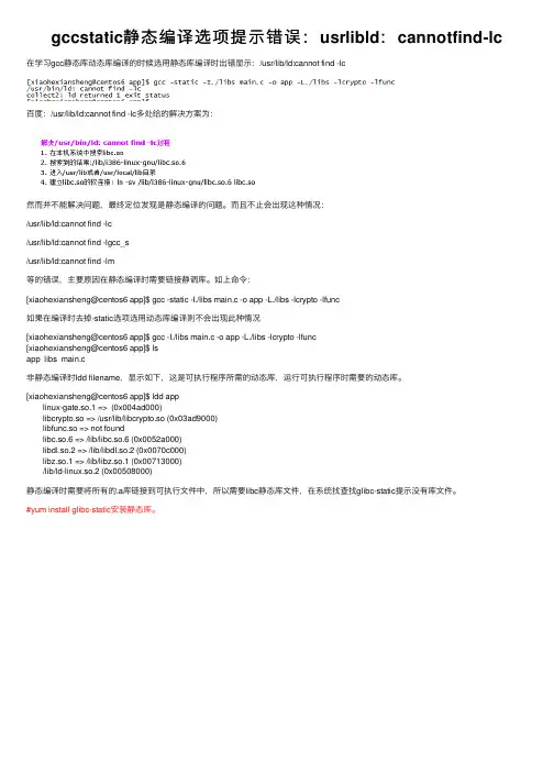
gccstatic静态编译选项提⽰错误:usrlibld:cannotfind-lc 在学习gcc静态库动态库编译的时候选⽤静态库编译时出错显⽰:/usr/lib/ld:cannot find -lc百度:/usr/lib/ld:cannot find -lc多处给的解决⽅案为:然⽽并不能解决问题,最终定位发现是静态编译的问题。
⽽且不⽌会出现这种情况:/usr/lib/ld:cannot find -lc/usr/lib/ld:cannot find -lgcc_s/usr/lib/ld:cannot find -lm等的错误,主要原因在静态编译时需要链接静调库。
如上命令:[xiaohexiansheng@centos6 app]$ gcc -static -I./libs main.c -o app -L./libs -lcrypto -lfunc如果在编译时去掉-static选项选⽤动态库编译则不会出现此种情况[xiaohexiansheng@centos6 app]$ gcc -I./libs main.c -o app -L./libs -lcrypto -lfunc[xiaohexiansheng@centos6 app]$ lsapp libs main.c⾮静态编译时ldd filename,显⽰如下,这是可执⾏程序所需的动态库,运⾏可执⾏程序时需要的动态库。
[xiaohexiansheng@centos6 app]$ ldd applinux-gate.so.1 => (0x004ad000)libcrypto.so => /usr/lib/libcrypto.so (0x03ad9000)libfunc.so => not foundlibc.so.6 => /lib/libc.so.6 (0x0052a000)libdl.so.2 => /lib/libdl.so.2 (0x0070c000)libz.so.1 => /lib/libz.so.1 (0x00713000)/lib/ld-linux.so.2 (0x00508000)静态编译时需要将所有的.a库链接到可执⾏⽂件中,所以需要libc静态库⽂件,在系统找查找glibc-static提⽰没有库⽂件。

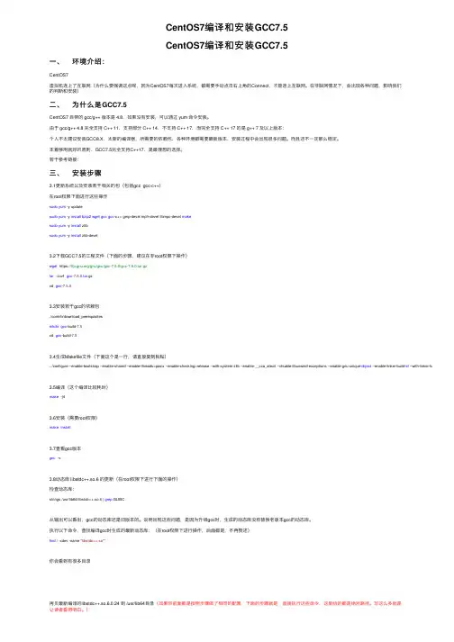
CentOS7编译和安装GCC7.5CentOS7编译和安装GCC7.5⼀、环境介绍:CentOS7虚拟机连上了互联⽹(为什么要强调这点呢,因为CentOS7每次进⼊系统,都需要⼿动点击右上⾓的Connect,才能连上互联⽹。
在⾮联⽹情况下,会出现各种问题,影响我们的判断和安装)⼆、为什么是GCC7.5CentOS7 ⾃带的 gcc/g++ 版本是 4.8,如果没有安装,可以通过 yum 命令安装。
由于 gcc/g++ 4.8 完全⽀持 C++ 11,⽀持部分 C++ 14,不⽀持 C++ 17,⽽完全⽀持 C++ 17 的是 g++ 7 及以上版本:个⼈不太建议安装GCC8.X,太新的编译器,所需要的依赖包、各种环境都需要最新版本,安装过程中会出现很多问题。
⽽且还不⼀定那么稳定。
本着够⽤就好的原则,GCC7.5完全⽀持C++17,是最理想的选择。
若⼲参考链接:三、安装步骤3.1更新系统以及安装若⼲相关的包(包括gcc gcc-c++)在root权限下⾯进⾏这些操作sudo yum -y updatesudo yum -y install bzip2wget gcc gcc-c++ gmp-devel mpfr-devel libmpc-devel makesudo yum -y install zlibsudo yum -y install zlib-devel3.2下载GCC7.5的⼯程⽂件(下⾯的步骤,建议在⾮root权限下操作)wget https:///gnu/gcc/gcc-7.5.0/gcc-7.5.0.tar.gztar -zxvf gcc-7.5.0.tar.gzcd gcc-7.5.03.3安装若⼲gcc的依赖包./contrib/download_prerequisitesmkdir gcc-build-7.5cd gcc-build-7.53.4⽣成Makefile⽂件(下⾯这个是⼀⾏,请直接复制粘贴)../configure --enable-bootstrap --enable-shared --enable-threads=posix --enable-checking=release --with-system-zlib --enable-__cxa_atexit --disable-libunwind-exceptions --enable-gnu-unique-object --enable-linker-build-id --with-linker-hash-style=gnu3.5编译(这个编译⽐较耗时)make -j43.6安装(需要root权限)make install3.7查看gcc版本gcc -v3.8动态库 libstdc++.so.6 的更新(在root权限下进⾏下⾯的操作)检查动态库:strings /usr/lib64/libstdc++.so.6 | grep GLIBC从输出可以看出,gcc的动态库还是旧版本的。
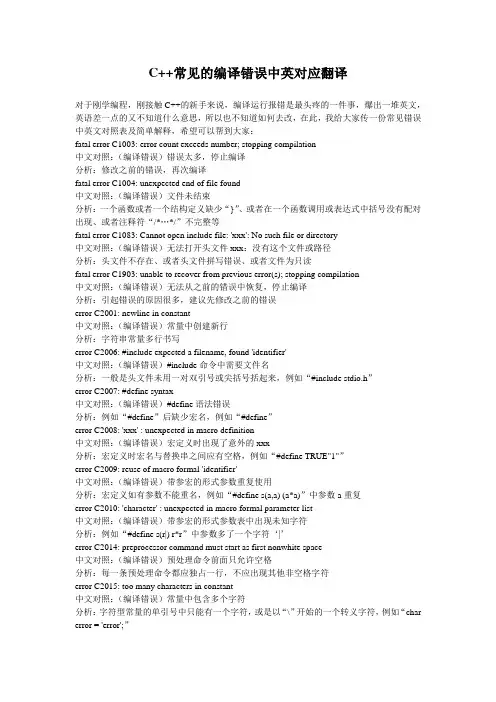
C++常见的编译错误中英对应翻译对于刚学编程,刚接触C++的新手来说,编译运行报错是最头疼的一件事,爆出一堆英文,英语差一点的又不知道什么意思,所以也不知道如何去改,在此,我给大家传一份常见错误中英文对照表及简单解释,希望可以帮到大家:fatal error C1003: error count exceeds number; stopping compilation中文对照:(编译错误)错误太多,停止编译分析:修改之前的错误,再次编译fatal error C1004: unexpected end of file found中文对照:(编译错误)文件未结束分析:一个函数或者一个结构定义缺少“}”、或者在一个函数调用或表达式中括号没有配对出现、或者注释符“/*…*/”不完整等fatal error C1083: Cannot open include file: 'xxx': No such file or directory中文对照:(编译错误)无法打开头文件xxx:没有这个文件或路径分析:头文件不存在、或者头文件拼写错误、或者文件为只读fatal error C1903: unable to recover from previous error(s); stopping compilation中文对照:(编译错误)无法从之前的错误中恢复,停止编译分析:引起错误的原因很多,建议先修改之前的错误error C2001: newline in constant中文对照:(编译错误)常量中创建新行分析:字符串常量多行书写error C2006: #include expected a filename, found 'identifier'中文对照:(编译错误)#include命令中需要文件名分析:一般是头文件未用一对双引号或尖括号括起来,例如“#include stdio.h”error C2007: #define syntax中文对照:(编译错误)#define语法错误分析:例如“#define”后缺少宏名,例如“#define”error C2008: 'xxx' : unexpected in macro definition中文对照:(编译错误)宏定义时出现了意外的xxx分析:宏定义时宏名与替换串之间应有空格,例如“#define TRUE"1"”error C2009: reuse of macro formal 'identifier'中文对照:(编译错误)带参宏的形式参数重复使用分析:宏定义如有参数不能重名,例如“#define s(a,a) (a*a)”中参数a重复error C2010: 'character' : unexpected in macro formal parameter list中文对照:(编译错误)带参宏的形式参数表中出现未知字符分析:例如“#define s(r|) r*r”中参数多了一个字符‘|’error C2014: preprocessor command must start as first nonwhite space中文对照:(编译错误)预处理命令前面只允许空格分析:每一条预处理命令都应独占一行,不应出现其他非空格字符error C2015: too many characters in constant中文对照:(编译错误)常量中包含多个字符分析:字符型常量的单引号中只能有一个字符,或是以“\”开始的一个转义字符,例如“char error = 'error';”error C2017: illegal escape sequence中文对照:(编译错误)转义字符非法分析:一般是转义字符位于' ' 或" " 之外,例如“char error = ' '\n;”error C2018: unknown character '0xhh'中文对照:(编译错误)未知的字符0xhh分析:一般是输入了中文标点符号,例如“char error = 'E';”中“;”为中文标点符号error C2019: expected preprocessor directive, found 'character'中文对照:(编译错误)期待预处理命令,但有无效字符分析:一般是预处理命令的#号后误输入其他无效字符,例如“#!define TRUE 1”error C2021: expected exponent value, not 'character'中文对照:(编译错误)期待指数值,不能是字符分析:一般是浮点数的指数表示形式有误,例如123.456Eerror C2039: 'identifier1' : is not a member of 'identifier2'中文对照:(编译错误)标识符1不是标识符2的成员分析:程序错误地调用或引用结构体、共用体、类的成员error C2041: illegal digit 'x' for base 'n'中文对照:(编译错误)对于n进制来说数字x非法分析:一般是八进制或十六进制数表示错误,例如“int i = 081;”语句中数字‘8’不是八进制的基数error C2048: more than one default中文对照:(编译错误)default语句多于一个分析:switch语句中只能有一个default,删去多余的defaulterror C2050: switch expression not integral中文对照:(编译错误)switch表达式不是整型的分析:switch表达式必须是整型(或字符型),例如“switch ("a")”中表达式为字符串,这是非法的error C2051: case expression not constant中文对照:(编译错误)case表达式不是常量分析:case表达式应为常量表达式,例如“case "a"”中“"a"”为字符串,这是非法的error C2052: 'type' : illegal type for case expression中文对照:(编译错误)case表达式类型非法分析:case表达式必须是一个整型常量(包括字符型)error C2057: expected constant expression中文对照:(编译错误)期待常量表达式分析:一般是定义数组时数组长度为变量,例如“int n=10; int a[n];”中n为变量,这是非法的error C2058: constant expression is not integral中文对照:(编译错误)常量表达式不是整数分析:一般是定义数组时数组长度不是整型常量error C2059: syntax error : 'xxx'中文对照:(编译错误)‘xxx’语法错误分析:引起错误的原因很多,可能多加或少加了符号xxxerror C2064: term does not evaluate to a function中文对照:(编译错误)无法识别函数语言分析:1、函数参数有误,表达式可能不正确,例如“sqrt(s(s-a)(s-b)(s-c));”中表达式不正确2、变量与函数重名或该标识符不是函数,例如“int i,j; j=i();”中i不是函数error C2065: 'xxx' : undeclared identifier中文对照:(编译错误)未定义的标识符xxx分析:1、如果xxx为cout、cin、scanf、printf、sqrt等,则程序中包含头文件有误2、未定义变量、数组、函数原型等,注意拼写错误或区分大小写。
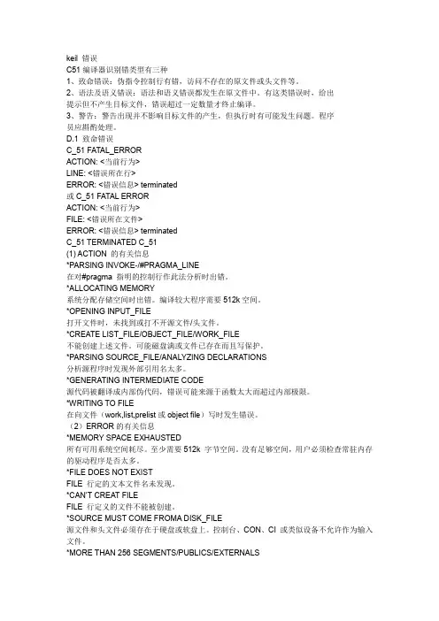
keil错误C51编译器识别错类型有三种1、致命错误:伪指令控制行有错,访问不存在的原文件或头文件等。
2、语法及语义错误:语法和语义错误都发生在原文件中。
有这类错误时,给出提示但不产生目标文件,错误超过一定数量才终止编译。
3、警告:警告出现并不影响目标文件的产生,但执行时有可能发生问题。
程序员应斟酌处理。
D.1 致命错误C_51 FATAL_ERRORACTION: <当前行为>LINE: <错误所在行>ERROR: <错误信息> terminated或C_51 FA TAL ERRORACTION: <当前行为>FILE: <错误所在文件>ERROR: <错误信息> terminatedC_51 TERMINATED C_51(1) ACTION 的有关信息*PARSING INVOKE-/#PRAGMA_LINE在对#pragma 指明的控制行作此法分析时出错。
*ALLOCATING MEMORY系统分配存储空间时出错。
编译较大程序需要512k空间。
*OPENING INPUT_FILE打开文件时,未找到或打不开源文件/头文件。
*CREATE LIST_FILE/OBJECT_FILE/WORK_FILE不能创建上述文件。
可能磁盘满或文件已存在而且写保护。
*PARSING SOURCE_FILE/ANALYZING DECLARATIONS分析源程序时发现外部引用名太多。
*GENERATING INTERMEDIATE CODE源代码被翻译成内部伪代码,错误可能来源于函数太大而超过内部极限。
*WRITING TO FILE在向文件(work,list,prelist或object file)写时发生错误。
(2)ERROR的有关信息*MEMORY SPACE EXHAUSTED所有可用系统空间耗尽。
至少需要512k 字节空间。
ActionScript 3.0编译器编译错误大全【转】以下是编译器遇到无效代码时生成的编译错误列表。
只有在严谨模式下编译代码时,才能检测到这些错误的子集。
严谨模式添加了标准语言中没有的三种约束:表达式有静态类型,且类型错误为验证错误。
附加验证规则捕获常见编程错误。
提前报告验证错误。
以下验证错误仅在严谨模式下出现:函数调用签名匹配,将检查所提供的参数数目及其类型。
重复定义冲突。
访问编译时未定义的方法或属性时出现未绑定的引用。
在密封对象上动态添加属性。
写入常量变量。
删除固定属性。
比较使用不兼容类型的表达式。
未找到包。
代码消息说明1000 对_ 的引用不明确。
引用可能指向多项。
例如,下面使用了rss 和xml 命名空间。
每个命名空间为hello() 函数定义了不同的值。
trace(hello()) 语句返回此错误,因为它无法确定使用哪个命名空间。
private nam espace rss; private namespace xml; public function ErrorExamples() { use namespace rss; use nam espace xml;trace(hello()); } rss function hello():String { return "hola"; } xml functionhello():String { return "foo"; }通过使用具体的引用来纠正不明确的引用。
下面的示例使用namespace::function 这种格式指定所要使用的命名空间:public function ErrorExamples() { trace(rss::hello()); trace(xml::hello()); }1003 不允许将访问说明符与命名空间属性结合使用。
不能在定义中同时使用访问说明符(如私有或公共)和命名空间属性。

C内存泄漏调试手段C内存泄漏调试手段在C语言开发中,内存泄漏是一种常见的问题。
当程序中申请的内存没有正确释放时,就会出现内存泄漏。
内存泄漏会导致程序运行效率低下,甚至引起系统崩溃。
因此,及时发现和修复内存泄漏是非常重要的。
下面介绍一些常用的C内存泄漏调试手段。
1. 静态分析工具静态分析工具可以在编译阶段对代码进行分析,检测出潜在的内存泄漏问题。
常用的静态分析工具包括Coverity、PVS-Studio等。
这些工具会对代码进行扫描,并给出可能存在的内存泄漏的警告或错误。
使用静态分析工具可以在编译前及时发现潜在的问题,提高代码质量。
2. 动态内存分析工具动态内存分析工具可以在程序运行时监测内存的分配和释放情况,帮助开发人员找出内存泄漏点。
常用的动态内存分析工具有Valgrind、Dr. Memory等。
这些工具会跟踪程序的内存分配和释放操作,并给出相应的报告。
通过分析报告,开发人员可以确定程序中存在的内存泄漏问题,并进行修复。
3. 日志输出在程序中添加日志输出可以帮助开发人员追踪内存分配和释放的情况。
可以在关键的代码段前后输出日志,用于检查内存分配和释放的情况。
通过日志输出,可以定位到内存泄漏的具体位置,并进行修复。
日志输出是一种简单但有效的调试手段。
4. 内存检测函数C语言提供了一些内存检测函数,可以帮助开发人员追踪内存的分配和释放情况。
例如,malloc函数用于申请内存,free函数用于释放内存。
通过在代码中添加适当的内存检测函数,可以检查内存的分配和释放是否正确。
如果发现内存没有正确释放,就可以确定存在内存泄漏,并进行修复。
5. 堆分析工具堆分析工具可以在程序运行时监测堆内存的分配和释放情况,帮助开发人员找出内存泄漏点。
常用的堆分析工具有Heaptrack、MemTrack等。
这些工具会记录堆内存的分配和释放操作,并给出相应的报告。
通过分析报告,开发人员可以确定程序中存在的内存泄漏问题,并进行修复。
FREE PASCAL出错信息对照表一、编译时的出错信息1.Out of memory [内存溢出]2.Identifier expected [缺标识符]3.Identifier not found [标识符未找到]*如:Identifier not found INTEGR [标识符INTEGER未找到]4.Duplicate identifier [重复说明]*如:Duplicate identifier N [变量N重复说明]5.Syntax error [语法错误]*6.Error in real constant [实型常量错]7.Error in integer constant [整型常量错]8.String constant exceeds line [字符串常量跨行]9.Too many nested file [文件嵌套过多]10.Unexpected end of file [非正常文件结束]11.Line to long [行过长]12.Type Identifier expected [缺类型标识符]13.Too many open file [打开文件过多]14.Invalid file name [无效文件名]15.File not found [文件未找到]*16.Disk full [磁盘满]17.Invalid compiler directive [无效编译指示]18.Too many file [文件过多]19.Undefined type in pointer definition [指针定义中未定义类型]20.Variable identifier expected [缺变量标识符]21.Error in type definition [类型错误说明]*22.Stucture too large [结构过长]23.Set base type out of range [集合基类型越界]24.File components may not be files or object [FILE分量不能为文件或对象]25.Invalid string length [无效字符串长度]26.Type mismatch [类型不匹配]*27.Invalid subrange base type [无效子界基类型]28.Lower bound greater than upper bound [下界大于上界]29.Ordinal type expected [缺有序类型]30.Integer constant expected [缺整型常数]31.Constant expected [缺常量]32.Integer or real constant expected [缺整型或实型常量]33.Pointe type identifier expected [缺指针类型标识符]34.Invalid function result type [无效的函数结果类型]bel identifier expected [缺标号标识符]36.Begin expected [缺BEGIN]*37.End expected [缺END]*38.Integer expression expected [缺整型表达式]39.Ordinal expression expected [缺有序表达式]40.Boolean expression expected [缺布尔表达式]41.Operand type do not match operator [操作数与操作符不匹配]42.Error in expression [表达式错]43.Illegal expression [非法赋值]*44.Field identifier expected [缺域标识符]45.Object file too large [目标文件过大]46.Undefined external [未定义外部标识符]47.Invalid object file record [无效OBJ文件记录]48.Code segment too large [代码段过长]49.Data segment too large [数据段过长]*50.Do expected [缺DO]*51.Invalid PUBLIC definition [无效PUBLIC定义]52.Invalid EXTRN definition [无效EXTRN定义]53.Too many EXTRN definition [EXTRN定义过多]54.Of extected [缺0F]*55.INTERFACE expected [缺INTERFACE]56.Invalid relocatable reference [无效重定位引用]57.THEN expected [缺THEN]*58.TO (DOWNTO) expected [缺T0或DOWNTO]*59.Undefined forward [提前引用未定义的说明]60.Too many procedures [过程过多]61.Invalid typecast [无效类型转换]62.Division by zero [被零除]63.Invalid typecast [无效文件类型]64.Cannot Read or Write variable of this type [不能读写该类型的变量]*65.Ponter variable expected [缺指针变量]66.String variable expected [缺字符串变量]67.String expression expected [缺字符串表达式]68.Circular unit reference [单元循环引用]69.Unit name mismatchg [单元名不匹配]70.Unit version mismatch [单元版本不匹配]71.Duplicate unit name [单元重名]72.Unit file format error [单元文件格式错误]73.Implementation expected [缺IMPLEMENTATl0N]74.constant and case types do not match [常数与CASE类型不相匹配]75.Record variable expected [缺记录变量]76.Constant out of range [常量越界]77.File variable expected [缺文件变量]78.Pointer extression expected [缺指针变量]79.Integer or real expression expected [缺整型或实型表达式]ble not within current block [标号不在当前块中]ble already defined [标号已定义]82.Undefined lable in preceding statement part [在前面语句中标号未定义]83.Invalid @ argument [无效的@参数]84.Unit expected [缺UNIT]85. “;” expected [缺“;”]*86. “:” expected [缺“:”]*87. “,” expected [缺“,”]*88. “(” expected [缺“(”)*89. “)” expected [缺“]” ]*90. “=” expected [缺“=”]*91. “:=” expected [缺“:=”]*92. “[” or “(” expected [缺“[”或“(”)*93. “]” or “)” expected [缺“]”或“)”]*94. “..” expected [缺“.”]*95. “..” expected [缺“..”]*96.Too many variable [变量过多]97.Invalid FOR control variable [无效FOR控制变量]98.Integer variable expected [缺整型变量]99.File and procedure types are not allowed here [此处不允许用文件和过程类型]100.Srting length mismatch [字符串长度不匹配]101.Invalid ordering of fields [无效域顺序]102.String constant expected [缺字符串常量]103.Integer or real variable expected [缺整型或实型变量]104.Ordinal variable expected [缺顺序变量]105.INLINE error [INLINE错]106.Character expression expected [缺字符表达式]107.Too many relocation items [重定位项过多]112.Case constant out of range [CASE常量越界]113.Error in statement [语句错]114.Can’t call an interrupt procedute [不能调用中断过程]116.Must be in 8087 mode to complie this [必须在8087方式下编译] 117.Target address not found [未找到目标地址]118.Include files are not allowed here [此处不允许包含INCLUDE文件] 120.NIL expected [缺NIL]121.Invalid qualifier [无效限定符]122.Invalid variable reference [无效变量引用]123.Too many symbols [符号过多]124.Statement part too large [语句部分过长]126.Files must be var parameters [文件必须为变量参数]127.Too many conditional directive [条件符号过多]128.Misplaced conditional directive [条件指令错位]129.ENDIF directive missing [缺少ENDIF 指令]130.Error in initial conditional defines [初始条件定义错]131.Header does not match previous definition [过程和函数头与前面定义的不匹配]132.Critical disk error [严重磁盘错误]133.Can’t evalute this expression [不能计算该表达式]*如:Can’t evalu te constart expression [不能计算该常量表达式] 134.Expression incorrectly terminated [表达式错误结束]135.Invaild format specifier [无效格式说明符]136.Invalid indirect reference [无效间接引用]137.Structed variable are not allowed here [此处不允许结构变量] 138.Can’t evalute without system u nit [无SYSTEM单元不能计算]139.Can’t access this symbols [不能存取该符号]140.Invalid floating –point operation [无效浮点运算]141. Can’t compile overlays to memory [不能将覆盖模块编译至内存] 142.Procedure or function variable expected [缺过程和函数变量]143.Invalid procedure or function reference. [无效过程或函数引用] 144.Can’t overlay this unit [不能覆盖该单元]147.Object type expected [缺对象类型]148.Local object types are not allowed [不允许局部对象类型]149.VIRTUAL expected [缺VIRTUAL]150.Method identifier expected [缺方法标识符]151.Virtual constructor are not allowed [不允许虚拟构造方法]152.Constructor Identifier expected [缺构造函数标识符]153.Destructor Identifier expected [缺析构函数标识符]154.Fail only allowed within constructors [FAIL标准过程只允许在构造方法内使用]155.Invalid combination of opcode and operands [无效的操作符和操作数组合]156.Memory reference expected [缺内存引用]157.Can’t add or subtrace relocatable symbols [不能加减可重定位符号] 158.Invalid register combination [无效寄存器组合]159.286/287 Instructions are not enabled [未激活286/287指令]160.Invalid symbol reference [无效符号引用]161.Code generation error [代码生成错]162.ASM expected [缺ASM]二、运行错误运行错误将显示错误信息,并终止程序的运行。
VC++编译器设置及错误一览VC++编译器设置错误可能很多人在安装VC 6.0后有过点击“Compile”或者“Build”后被出现的“Compiling... ,Error spawning cl.exe”错误提示给郁闷过。
很多人的选择是重装,实际上这个问题很多情况下是由于路径设置的问题引起的,“CL.exe”是VC使用真正的编译器(编译程序),其路径在“VC根目录\VC98\Bin”下面,你可以到相应的路径下找到这个应用程序。
因此问题可以按照以下方法解决:打开vc界面点击VC“TOOLS(工具)”—>“Option (选择)”—>“Directories (目录)”重新设置“Excutable Fils、Include Files、Library Files、Source Files”的路径。
很多情况可能就一个盘符的不同(例如你的VC装在C,但是这些路径全部在D),改过来就OK了。
如果你是按照初始路径安装vc6.0的,路径应为:executatble files:C:\Program Files\Microsoft Visual Studio\Common\MSDev98\BinC:\Program Files\Microsoft Visual Studio\VC98\BINC:\Program Files\Microsoft Visual Studio\Common\TOOLS C:\Program Files\Microsoft Visual Studio\Common\TOOLS\WINNTinclude files:C:\Program Files\Microsoft Visual Studio\VC98\INCLUDEC:\Program Files\Microsoft Visual Studio\VC98\MFC\INCLUDEC:\Program Files\Microsoft Visual Studio\VC98\ATL\INCLUDElibrary files:C:\Program Files\Microsoft Visual Studio\VC98\LIBC:\Program Files\Microsoft Visual Studio\VC98\MFC\LIBsource files:C:\Program Files\Microsoft Visual Studio\VC98\MFC\SRCC:\Program Files\Microsoft Visual Studio\VC98\MFC\INCLUDEC:\Program Files\Microsoft Visual Studio\VC98\ATL\INCLUDEC:\Program Files\Microsoft Visual Studio\VC98\CRT\SRC如果你装在其他盘里,则仿照其路径变通就行(我就是装在D盘)。
编译时错误信息错误代码及错误信息错误释义error 1: Out of memory 内存溢出error 2: Identifier expected 缺标识符error 3: Unknown identifier 未定义的标识符error 4: Duplicate identifier 重复定义的标识符error 5: Syntax error 语法错误error 6: Error in real constant 实型常量错误error 7: Error in integer constant 整型常量错误error 8: String constant exceeds line 字符串常量超过一行error 10: Unexpected end of file 文件非正常结束error 11: Line too long 行太长error 12: Type identifier expected 未定义的类型标识符error 13: Too many open files 打开文件太多error 14: Invalid file name 无效的文件名error 15: File not found 文件未找到error 16: Disk full 磁盘满error 17: Invalid compiler directive 无效的编译命令error 18: Too many files 文件太多error 19: Undefined type in pointer def 指针定义中未定义类型error 20: V ariable identifier expected 缺变量标识符error 21: Error in type 类型错误error 22: Structure too large 结构类型太长error 23: Set base type out of range 集合基类型越界error 24: File components may not be files or objectsfile 分量不能是文件或对象error 25: Invalid string length 无效的字符串长度error 26: Type mismatch 类型不匹配error 27: error 27: Invalid subrange base type 无效的子界基类型error 28: Lower bound greater than upper bound 下界超过上界error 29: Ordinal type expected 缺有序类型error 30: Integer constant expected 缺整型常量error 31: Constant expected 缺常量error 32: Integer or real constant expected 缺整型或实型常量error 33: Pointer Type identifier expected 缺指针类型标识符error 34: Invalid function result type 无效的函数结果类型error 35: Label identifier expected 缺标号标识符error 36: BEGIN expected 缺BEGINerror 37: END expected 缺ENDerror 38: Integer expression expected 缺整型表达式error 39: Ordinal expression expected 缺有序类型表达式error 40: Boolean expression expected 缺布尔表达式error 41: Operand types do not match 操作数类型不匹配error 42: Error in expression 表达式错误error 43: Illegal assignment 非法赋值error 44: Field identifier expected 缺域标识符error 45: Object file too large 目标文件太大error 46: Undefined external 未定义的外部过程与函数error 47: Invalid object file record 无效的OBJ文件格式error 48: Code segment too large 代码段太长error 49: Data segment too large 数据段太长error 50: DO expected 缺DOerror 51: Invalid PUBLIC definition 无效的PUBLIC定义error 52: Invalid EXTRN definition 无效的EXTRN定义error 53: Too many EXTRN definitions 太多的EXTRN定义error 54: OF expected 缺OFerror 55: INTERFACE expected 缺INTERFACEerror 56: Invalid relocatable reference 无效的可重定位引用error 57: THEN expected 缺THENerror 58: TO or DOWNTO expected 缺TO或DOWNTO error 59: Undefined forward 提前引用未经定义的说明error 61: Invalid typecast 无效的类型转换error 62: Division by zero 被零除error 63: Invalid file type 无效的文件类型error 64: Cannot read or write variables of this type 不能读写此类型变量error 65: Pointer variable expected 缺指针类型变量error 66: String variable expected 缺字符串变量error 67: String expression expected 缺字符串表达式error 68: Circular unit reference 单元UNIT部件循环引用error 69: Unit name mismatch 单元名不匹配error 70: Unit version mismatch 单元版本不匹配error 71: Internal stack overflow 内部堆栈溢出error 72: Unit file format error 单元文件格式错误error 73: IMPLEMENTATION expected 缺IMPLEMENTA TION error 74: Constant and case types do not match 常量和CASE类型不匹配error 75: Record or object variable expected 缺记录或对象变量error 76: Constant out of range 常量越界error 77: File variable expected 缺文件变量error 78: Pointer expression expected 缺指针表达式error 79: Integer or real expression expected 缺整型或实型表达式error 80: Label not within current block 标号不在当前块内error 81: Label already defined 标号已定义error 82: Undefined label in preceding statement part 在前面未定义标号error 83: Invalid @ argument 无效的@参数error 84: UNIT expected 缺UNITerror 85: ";" expected 缺“;”error 86: ": " expected 缺“:”error 87: "," expected 缺“,”error 88: "(" expected 缺“(”error 89: ")" expected 缺“)”error 90: "=" expected 缺“=”error 91: ":=" expected 缺“:=”error 92: "[" or "(." Expected 缺“[”或“(.”error 93: "]" or ".)" expected 缺“]”或“.)”error 94: "." expected 缺“.”error 95: ".." expected 缺“..”error 96: Too many variables 变量太多error 97: Invalid FOR control variable 无效的FOR循环控制变量error 98: Integer variable expected 缺整型变量error 99: Files and procedure types are not allowed here 该处不允许文件和过程类型error 100: String length mismatch 字符串长度不匹配error 101: Invalid ordering of fields 无效域顺序error 102: String constant expected 缺字符串常量error 103: Integer or real variable expected 缺整型或实型变量error 104: Ordinal variable expected 缺有序类型变量error 105: INLINE error INLINE错误error 106: Character expression expected 缺字符表达式error 107: Too many relocation items 重定位项太多error 108: Overflow in arithmetic operation 算术运算溢出error 112: CASE constant out of range CASE常量越界error 113: Error in statement 表达式错误error 114: Cannot call an interrupt procedure 不能调用中断过程error 116: Must be in 8087 mode to compile this 必须在8087模式编译error 117: Target address not found 找不到目标地址error 118: Include files are not allowed here 该处不允许INCLUDE文件error 119: No inherited methods are accessible here 该处继承方法不可访问error 121: Invalid qualifier 无效的限定符error 122: Invalid variable reference 无效的变量引用error 123: Too many symbols 符号太多error 124: Statement part too large 语句体太长error 126: Files must be var parameters 文件必须是变量形参error 127: Too many conditional symbols 条件符号太多error 128: Misplaced conditional directive 条件指令错位error 129: ENDIF directive missing 缺ENDIF指令error 130: Error in initial conditional defines 初始条件定义错误error 131: Header does not match previous definition 和前面定义的过程或函数不匹配error 133: Cannot evaluate this expression 不能计算该表达式error 134: Expression incorrectly terminated 表达式错误结束error 135: Invalid format specifier 无效格式说明符error 136: Invalid indirect reference 无效的间接引用error 137: Structured variables are not allowed here 该处不允许结构变量error 138: Cannot evaluate without System unit 没有System单元不能计算error 139: Cannot access this symbol 不能存取符号error 140: Invalid floating point operation 无效的符号运算error 141: Cannot compile overlays to memory 不能编译覆盖模块至内存error 142: Pointer or procedural variable expected 缺指针或过程变量error 143: Invalid procedure or function reference 无效的过程或函数调用error 144: Cannot overlay this unit 不能覆盖该单元error 146: File access denied 不允许文件访问error 147: Object type expected 缺对象类型error 148: Local object types are not allowed 不允许局部对象类型error 149: VIRTUAL expected 缺VIRTUALerror 150: Method identifier expected 缺方法标识符error 151: Virtual constructors are not allowed 不允许虚构造函数error 152: Constructor identifier expected 缺构造函数标识符error 153: Destructor identifier expected 缺析构函数标识符error 154: Fail only allowed within constructors Fail标准过程只能用于构造函数error 155: Invalid combination of opcode and operands 操作数与操作符无效组合error 156: Memory reference expected 缺内存引用指针error 157: Cannot add or subtract relocatable symbols 不能加减可重定位符号error 158: Invalid register combination 无效寄存器组合error 159: 286/287 instructions are not enabled 未激活286/287指令error 160: Invalid symbol reference 无效符号指针error 161: Code generation error 代码生成错误error 162: ASM expected 缺ASMerror 166: Procedure or function identifier expected 缺过程或函数标识符error 167: Cannot export this symbol 不能输出该符号error 168: Duplicate export name 外部文件名重复error 169: Executable file header too large 可执行文件头太长error 170: Too many segments 段太多运行错误信息运行错误分为四类:1、1-99为DOS错误;2、100-149为I/O错误。
VC中常见的一些编译链接错误的解决问题1:Linking...nafxcwd.lib(thrdcore.obj) : error LNK2001: unresolved external symbol __endthreadexnafxcwd.lib(thrdcore.obj) : error LNK2001: unresolved external symbol __beginthreadexlibcd.lib(crt0.obj) : error LNK2001: unresolved external symbol _main答VC++默认的工程设置是单线程的,而你使用了多线程,所以要修改设置。
选择菜单“Project|settings”,选择C/C++标签,在CODEGENERATION分类中选择除SINGLE-THREADED的其他选择。
比如可以在Use run-time library中选择Debug Multithreaded 或者multithreaded其中,Single-Threaded 单线程静态链接库(release版本)Multithreaded 多线程静态链接库(release版本)multithreaded DLL 多线程动态链接库(release版本)Debug Single-Threaded 单线程静态链接库(debug版本)Debug Multithreaded 多线程静态链接库(debug版本)Debug Multithreaded DLL 多线程动态链接库(debug版本)单线程: 不需要多线程调用时, 多用在DOS环境下多线程: 可以并发运行静态库: 直接将库与程序Link, 可以脱离MFC库运行动态库: 需要相应的DLL动态库, 程序才能运行release版本: 正式发布时使用debug版本: 调试阶段使用问题2fatal error C1010: unexpected end of file while looking for precompiled header directive该如何解如果发生错误的文件是由其他的C代码文件添加进入当前工程而引起的,则Alt+F7进入当前工程的Settings,选择C/C++选项卡,从Category组合框中选中Precompiled Headers,选择Not Using Precompiled headers。
C#程序代码编译时常用的命令时间:2009-05-31 20:02:54来源:网络作者:未知点击:0次CSC.exe把Visual C#程序代码编译成IL文件时,有着很多参数和开关选项。
正确的了解和运用这些参数和开关有时会解决一些看似很棘手的问题。
下面就通过一张表来大致说明一下这些参数和开关的具体作用。
这些参数和开关选CSC.exe把Visual C#程序代码编译成IL文件时,有着很多参数和开关选项。
正确的了解和运用这些参数和开关有时会解决一些看似很棘手的问题。
下面就通过一张表来大致说明一下这些参数和开关的具体作用。
这些参数和开关选项是按照字母顺序来排列的。
其中带"*",是一些常用的参数或开关。
选项用途@ * 指定响应文件。
/?, /help 在控制台的计算机屏幕上显示编译器的选项/addmodule 指定一个或多个模块为集会的一部分/baseaddress指定装入DLL的基础地址/bugreport 创建一个文件,该文件包含是报告错误更加容易的信息/checked 如果整数计算溢出数据类型的边界,则在运行时产生一个例外的事件/codepage 指定代码页以便在编译中使用的所有源代码文件/debug * 发送调试信息/define 定义预处理的程序符号/doc * 把处理的文档注释为XML文件/fullpaths 指定编译输出文件的反正路径/incremental 对源代码的文件进行增量编译/linkresource 把.NET资源链接到集合中/main 指定Main方法的位置/nologo 禁止使用编译器的标志信息/nooutput 编译文件但不输出文件/nostdlib 不导出标准库(即mscorlib.dll)/nowarn 编译但编译器并不显示警告功能/optimize 打开或者关闭优化/out * 指定输出文件/recurse 搜索编译源文件的子目录/reference * 从包含集合的文件中导入元数据/target * 指定输出文件的格式/unsafe 编译使用非安全关键字的代码/warn 设置警告级别/warnaserror 提升警告为错误/win32icon 插入一个.ico文件导输出文件中去/win32res 插入一个Win32资源导输出文件中具体说明:一.@这个选项是用来指定响应文件。
Making plain binary files using a C compiler (i386+)作者:Cornelis Frank April 10, 2000翻译:coly li我写这篇文章是因为在internet上关于这个主题的信息很少,而我的EduOS项目又需要它。
对于由此文中信息所引申、引起的意外或不利之处,作者均不负有任何责任。
如果因为我的糟糕英语导致你的机器故障,那是你的问题,而不是我的。
1,你需要什么工具一个i386或者更高x86CPU配置的PC一个Linux发行版本,Redhat或者Slackware就不错。
一个GNU GCC编译器。
一般linux发行版本都会自带,可以通过如下命令检查你的GCC的版本和类型:gcc --version这将会产生如下的输出:2.7.2.3可能你的输出和上面的不一样,但是这不碍事。
Linux下的binutils工具包。
NASM 0.97或者更高的版本汇编器。
Netwide Assembler,即NASM,是一个80x86的模块化的可移植的汇编器。
他支持一系列的对象文件格式,包括linux的”a.out”,和ELF,NetBSD/FreeBSD,COFF,Microsoft 16位OBJ和Win32。
他也可以输出无格式二进制文件。
他的语法设计的非常简单并且易于理解,同intel的非常相似但是没有那么复杂。
它支持Pentium,P6和MMX操作数,并且支持宏。
如果你的机器上没有NASM,可以从下述网站下载:/pub/Linux/devel/lang/assemblers/一个象emacs或者pico那样的文本编辑器。
1.1安装Netwide汇编器(NASM)假定当前目录下存有nasm-0.97的压缩包,输入:gunzip nasm-0.97.tar.gztar -vxf nasm-0.97.tar这将建立一个名为nasm-0.97的目录,进入这个目录,下一步我们将输入如下命令来编译这个汇编器:./configuremake这将建立可执行文件nasm和ndisasm。
QT MinGW在windows中静态编译程序QT+MinGW在windows中静态编译程序2010年06月30日星期三19:45版本1:为什么要静态编译?如果不是静态编译程序,那我们写的程序文件编译生成可执行文件必须依赖QT和MinGW的一些库文件,虽然我们可以将这些依赖的dll文件一同打包发布,但毕竟看起来不是很好看,而且库内有的东西我们根本用不到,还是要复制整个dll,造成程序发布包比较大。
那么,怎么才能使我们的程序在没有安装QT和MinGW的系统上照样运行呢?首先,要保证QT是静态编译版本。
一般我们用的QT都不是静态编译的,需要我们重新编译。
在开始菜单里打开"Qt 4.x.x Command Prompt",这时默认是在QT目录里面,分别运行如下命令:configure-release-static-fast make make clean最后一部其实也算可有可无,第二步在我的电脑上运行了将近3个小时,慢慢等就是。
这样就生成了QT的静态编译版本,我们的程序编译时会自动把QT相关的依赖包含进去。
其次,解决MinGW的mingwm10.dll依赖问题。
一般只有用到threads 的时候才用到mingwm10.dll,我们通常遇到的"缺少mingwm10.dll"问题,可以在程序qmake生成makefile.release文件后删除"-mthreads"参数即可,一般在"LFLAGS"后面。
当然,这只是临时解决方案,每次都要手动修改,也可以在编译QT前先修改qmake.h,不过不推荐这种方法。
其实,mingwm10.dll也就十多K,每次发布程序时一起打包也无所谓。
更多信息可以参考:.381-0.html#msg00553这样编译出来的程序比较大,可以先用strip命令去掉程序里面一些无用信息后,用ASPack或者UPX之类的压缩加壳软件压缩一下,两者的压缩率基本都达到30%多一点,压缩效果还是很明显的。
DELPHI的编译指令{$IFDEF WIN32} -- 这可不是批注喔!对于Delphi来说﹐左右大括号之间的内容是批注﹐然而「{$」(左括号后紧接着货币符号)对于Compiler(编译器)而言并不是批注﹐而是写给Compiler看的特别指示。
应用时机与场合Delphi中有许许多多的Compiler Directives(编译器指令)﹐这些编译指令对于我们的程序发展有何影响呢? 它们又能帮我们什么忙呢?Compiler Directive 对程序开发的影响与助益, 可以从以下几个方向来讨论:协助除错版本分类程序的重用与管理设定统一的执行环境协助除错稳健熟练的程序设计师经常会在开发应用系统的过程中﹐特别加入一些除错程序或者回馈验算的程序﹐这些除错程序对于软件品质的提升有极其正面的功能。
然而开发完成的正式版本中如果不需要这些额外的程序的话﹐要想在一堆程序中找出哪些是除错用的程序并加以删除或设定为批注﹐不仅累人﹐而且容易出错﹐况且日后维护时这些除错程序还用得着。
此时如果能够应用像是$IFDEF的Compiler Directives ﹐就可以轻易的指示Delphi要/不要将某一段程序编进执行文件中。
同时﹐Compiler本身也提供了一些错误检查的开关﹐可以预先对程序中可能的问题提醒程序设计师注意﹐同样有助于撰写正确的程序。
版本分类除了上述的除错版本/正式版本的分类之外﹐对于像是「试用版」「普及版」「专业版」的版本分类﹐也可以经由Compiler Directive的使用﹐为最后的产品设定不同的使用权限。
其它诸如「中文版」「日文版」「国际标准版」等全球版本管理方面﹐同样也可以视需要指示Delphi特别连结哪些资源档或者是采用哪些适当的程序。
以上的两则例子中﹐各版本间只需共享同一份程序代码即可。
Delphi 1.0 与Delphi 2.0有许多不同之处﹐组件资源文件(.DCR)即是其中一例﹐两者的档案格式并不兼容﹐在您读过本文之后﹐相信可以写出这样的程序﹐指示Delphi在不同的版本采用适当的资源文件以利于组件的安装。
expecting member declaratio “expecting member declaration”是一个编程错误,通常出现在C++或其他类似的面向对象的编程语言中。
这个错误意味着编译器在类的定义中期望找到一个成员声明,但是没有找到。
这通常是因为在类的主体中写了一些不应该出现的东西,或者忘记了在类的主体中写任何东西。
这里有一些可能导致“expecting member declaration”错误的常见原因:语法错误:在类的主体中,你可能不小心写了一些不符合语法的代码。
例如,你可能忘记了在成员函数的声明后面加上分号。
缺少成员声明:你可能只定义了一个空的类主体,而没有在里面声明任何成员。
虽然这在语法上是允许的,但通常不是一个好的做法,因为它创建了一个没有实际用途的类。
错误的成员声明:你可能试图在类的主体中声明一些不应该出现的东西,比如另一个类的定义或者一个全局变量的声明。
为了解决这个问题,你需要检查你的类定义,并确保所有的成员声明都是正确的,并且符合语法规则。
如果你不确定如何修复这个错误,你可以查阅相关的编程文档,或者在网上搜索类似的错误信息以找到解决方案。
这里有一个简单的C++类定义的例子,它应该不会导致“expecting member declaration”错误:cppclass MyClass {public:int myMemberVariable; // 成员变量声明void myMemberFunction(); // 成员函数声明};// 成员函数的定义可以在类的外部进行void MyClass::myMemberFunction() {// 这里是函数的实现}在这个例子中,MyClass 类有一个成员变量 myMemberVariable 和一个成员函数 myMemberFunction。
注意在类的主体中,成员函数的实现是被省略的,通常会在类的外部进行定义和实现。
IAR中头文件路径配置IAR中头文件路径配置Error[Cp001]: Copy protection check, No valid license found for this product [20]原因:安装的时候没有把注册机的0x.....字串的小写字母改为大写字母。
Warning[Pe001]: last line of file ends without a newline F:/emoTion/IAR/PK 升级/CC1110-8/main.c原因:在使用IAR时常常会弹出类似这样一个警告,其实只要在最后一行多加一个回车就不会再有这个警告了.Error[e72]: Segment BANK_RELAYS must be defined in a segment definition option (-Z, -b or -P) 原因:这是用730B编译的错误,可能是由于相对于目标工程版本过高的,后改用720H,没有发生错误。
Error[Pe005]: could not open source file "stdio.h"原因:头文件路径不对造成,改正的方法是在设置选项卡的C/C++ Compiler -> Preprocessor 选项里,将$TOOLKIT_DIR$/INC/CLIB/添到Include paths中。
Error[Pe005]: could not open source file "hal.h" C:/Users/user/Desktop/例子程序/无线通信综合测试/Library/cc2430/HAL/source/setTimer34Period.c原因:先检查C:/Users/user/Desktop/例子程序/无线通信综合测试/Library/cc2430/HAL/source/有无setTimer34Period.c这个文件,若有,则是因为IAR对中文路径支持不好的缘故,把这个工程复制到英文路径下编译就不会发生错误。
Compiler-Directed Static Classification of Value Locality BehaviorQing Zhao and David J. Lilja∗Dept. of Computer Science and Engineering, Univ. of Minnesota, Minneapolis, MN 55455∗Dept. of Electrical and Computer Engineering, Univ. of Minnesota, Minneapolis, MN 55455zhao@, ∗lilja@AbstractPredicting the values that are likely to be produced by instructions has been suggested as a way of increasing the instruction-level parallelism available in a wide-issue processor. One of the potential difficulties in exploiting the predictability of values, however, is selecting the proper type of predictor, such as a last-value predictor, a stride predictor, or a context-based predictor, for a given instruction. We propose a compiler-directed classification scheme that statically partitions all of the instructions in a program into several groups, each of which is associated with a specific value predictability pattern. This value predictability pattern is encoded into the instructions to identify the type of value predictor that will be best suited for predicting the values that are likely to be produced by each instruction at run-time. Both an idealized profile-based compiler implementation and an implementation based on the GCC compiler are studied to show the performance bounds for the proposed technique. Our simulations based on the SimpleScalar tool set and the SPEC95 integer benchmarks indicate that this approach can substantially reduce the number of read/write ports needed in the value predictor for a given level of performance. This static partitioning approach also produces better performance than a dynamically partitioned approach for a given hardware configuration. Finally, this work demonstrates the connection between value locality behavior and source-level program structures thereby leading to a deeper understanding of the causes of this behavior.1 IntroductionSeveral constraints limit the instruction-level parallelism (ILP) that can be exploited in programs, including true data dependencies (read-after-write hazards), artificial dependencies (write-after-read and write-after-write hazards), control dependencies (branches), and resource conflicts (such as limited numbers of register ports or function units). While the performance impact of control dependencies and artificial dependencies can be reduced or sometimes even eliminated using various hardware and software techniques, such as branch prediction and register renaming, true data dependencies remain a serious limitation in exploiting ILP in superscalar processors. Value prediction has been proposed as a mechanism to break true data dependencies [2,3, 6-15].Recent studies have shown that wide-issue processors benefit more from value prediction than traditional four-instruction-issue superscalar processors since more true data dependencies typically appear in the larger instruction windows needed to support wider issue widths [2]. Eliminating datadependencies in these larger instruction windows potentially can increase performance substantially. On the other hand, several problems arise when applying value prediction in wide-issue processors. For instance, since multiple instructions need to access the value predictor in each cycle, the predictors must be able to support very high read/write bandwidths. Our measurements on a set of SPEC95 integer programs, which are summarized in Table 1, show that a simple value predictor (the SVP described in Section 4.3) must support an average of 5 accesses per cycle for an 8-issue processor, increasing to 7 accesses per cycle for a 16-issue processor. If the value predictor is unable to support this request bandwidth, many predictions that could otherwise have been made will not be available to the instruction issue logic. Furthermore, entries in the value predictor will not be updated with the newly generated values in time for the next prediction request, which will cause a corresponding increase in the misprediction rate.benchmarksissue widthgo m88ksim gcc compress li ijpeg perl vortex AVG 8_issue 5.2 5.5 4.6 5.2 4.5 6.1 4.7 4.2 5.016_issue 6.110.7 6.3 6.7 6.311.0 6.1 6.07.0Table 1. The average number of requests per cycle made to a simple value predictor in a wide-issuesuperscalar processor.There are several approaches that can be used to resolve this value prediction bandwidth problem. A straightforward approach is to increase the number of read/write ports in the value predictor. While multiple independent ports will increase the number of requests per cycle that can be handled by the predictor, each additional port increases the complexity of the design with additional decoding and multiplexing logic and, perhaps more importantly, it substantially increases the wiring density. This additional circuitry and increased wire density will increase the implementation cost. Furthermore, these changes most likely increase the critical path delays, which then will increase the predictorÕs access time and the processorÕs clock period. A variation of this approach interleaves the predictor using several banks with a fast distribution network [2]. This scheme still suffers from bank conflicts, however, since several instructions may try to access the same bank simultaneously. Moreover, this interleaving requires a scaling factor that is a power of two, which severely restricts the development of a cost-effective design for value predictors in high-issue width processors [4].A decoupled value predictor scheme has been proposed [3] that reduces the bandwidth requirement of the predictor by dynamically classifying each instruction into one of several different componentpredictors. One drawback of this scheme, though, is that it requires a modified trace cache to store the classification information for each instruction. Additionally, this dynamic classification scheme suffers from a relatively long latency required to classify instructions. Due to changes in the predictability behavior of some instructions during a programÕs execution, these instructions migrate among the several different component predictors at run-time. These frequent migrations will introduce many transient states into the predictors, thereby reducing their effectiveness.This paper proposes a new compiler-directed classification scheme for statically partitioning individual instructions among several different component value predictors. The compiler attaches information about the value predictability pattern for each instruction to its binary object code through a simple extension of the instruction format. This compiler-directed static classification scheme reduces the hardware cost and complexity required to build a large prediction cache with multiple ports. Instead, several smaller value predictors with only a limited number of ports in each can provide the equivalent bandwidth of a single larger multiported predictor while maintaining approximately the same, and in some cases even slightly better, prediction accuracy. Since each instruction is statically marked with its prediction classification, no additional hardware classification table is needed. This preclassification also eliminates the time required by existing dynamic classification schemes to classify the value predictability behavior of instructions and it eliminates the start-up overhead incurred when instructions migrate among several different component predictors. It also eliminates the need for a single instruction to occupy multiple entries simultaneously in the component predictors of the overall predictor.Unlike other compiler-directed techniques that rely on profile-guided heuristics [5], our static classification scheme identifies the salient characteristics of predictable instructions at compile time without the need to profile the program beforehand.The remainder of this paper is organized as follows: Section 2 summarizes recent related work on value prediction schemes. Section 3 then studies the inherent characteristics of programs that serve as the basis for the static classification. This section also describes the compiler classification heuristics and presents classification results for an idealized compiler. Our performance evaluation methodology is described in Section 4 with the simulation results presented in Section 5. Finally, the results and conclusions are summarized in Section 6.2 Related WorkThere are three main areas of previous work related to the scheme proposed in this paper. The first area focuses on building more accurate and efficient value predictors, such as the last-value predictor [6], the stride value predictor [7], and the context-based value predictor [8,9]. Each of these predictors produces good performance for certain value locality patterns, but poor performance for others. To obtain higher prediction rates for instructions with varying value locality patterns, several simple value predictors can be combined into one hybrid value predictor [9,10,11]. Although these hybrid value predictors can provide higher prediction rate than single predictors, they can waste resources since every instruction being predicted occupies a unique entry in each of the component predictors. To address this inefficient use of the predictor resources, dynamic classification schemes [3,10,11] can distribute the instructions into the different component predictors at run-time.Another important area of related work has studied how to incorporate value predictors in complete machine models. Gabbay and Mendelson [2] showed that the performance potential of value prediction tends to increase as the instruction issue width increases. However, it has been pointed out [2,3] that using value prediction in wide-issue processors requires very high bandwidth predictors. To address this problem, a highly interleaved prediction table has been proposed [2]. Additionally, Lee et al [3] combined a dynamic classification table with a trace cache to distribute instructions to different component predictors thereby increasing the predictor bandwidth available in each cycle. Another approach is to reduce the bandwidth requirement of the predictors by giving priority to those instructions that belong to the longest data dependence chains [12]. Rychlic et al [11] have shown that over 30% of the value predictions in the SPEC95 integer programs produced no performance improvement, which further supports the selective prediction scheme.Finally, the last area of important related work has studied the program characteristics that lead to value locality [14,15]. For instance, Sazeides and Smith [14] divided prediction models into two groups, computational and context-based, while Sodani and Sohi [15] studied the sources of instruction repetition at both the global level and the local level.3. Static ClassificationA program's execution-time behavior determines the predictability of the values its instructions produce. There are two basic types of value predictability in programs [14]:•Value repetition, in which subsequent dynamic instances of the same static instruction repeat the values produced by previous dynamic instances. The repetition distance is the number of times an instruction is executed between two repetitions of the same value (including the repeating instance itself). For instance, an instruction that always produces the same value has a repetition distance of one, while an instruction that alternately produces only two distinct values has a repetition distance of two. Note that the repetition distance need not be constant for a particular static instruction.•Value computability, in which values produced by later dynamic instances of the same static instruction can be computed using a simple function of the previous values.Last-value predictors [6] and context-based value predictors [8,9] have been proposed to capture the value repetition that exists in programs. The primary difference between these two types of predictors is the repetition distance that can be exploited by each. The last-value predictors assume that the immediately previous value produced by an instruction will be produced again the next time it is executed. Thus, it assumes a repetition distance of one. The context-based predictors, on the other hand, generalize to arbitrary repetition distances by selecting one of several previous values as the next value predicted to be produced by an instruction. Computational predictors, such as the stride value predictor [7], compute the next predicted value using some predefined function of previously seen values, such as an increment by a constant stride.In this section, we further categorize the predictability behavior of instructions with the goal of developing compiler algorithms to statically identify the value predictability pattern of each instruction. 3.1 Value Predictability Patterns for Static InstructionsWe classify static instructions into three different groups according to the predictability behavior that they exhibit. This classification was developed by observing both the run-time behavior of programs and the source code level structures that can be naturally analyzed by compilers.•Single_Pattern -- These instructions have exactly one type of value predictability during the execution of the program. For example, the sequence {1, 2, 3, 4, 5, 6, ...} demonstrates a computable value predictability pattern while the sequence {4, 7, 9, 4, 7, 9, ...} shows a single type of value repetition.We further subdivide this group below.•Mixed_Pattern -- Instructions with this category may interleave both the value repetition and the value computability types of behavior. The value sequence {1, 2, 3, 5, 5, 5, 5, 1, 2, 3, 5, 5, ...}, for instance, shows both repetition of values and a stride-based computable pattern.•Unknown -- This group includes static instructions whose values are not predictable during the program execution.It is useful to further divide static instructions in the Single_Pattern group into the following three subgroups:•The Single_Last subgroup includes those instructions that have a constant repetition distance of one.That is, the instruction usually produces the same value as the immediately previous instance.•The Single_Stride subgroup includes instructions whose values are computable using a constant stride.•The Single_Context subgroup includes instructions with a value repetition distance larger than one.For example, the dynamic instruction instances sequence {1, 4, 17, 23, 1, 4, 17, 23, 1, ...} exhibits value repetition with a repetition distance of four. The corresponding static instruction thus belongs to this Single_Context subgroup.Note that static instructions in both the Single_Last and Single_Context subgroups show similar value repetition behavior, differing only in the repetition distance. Logically, they could be combined into a single group with an associated value repetition distance. However, the Single_Last type is pulled out as a separate subgroup because instructions with this behavior occur quite frequently in the programs tested.Each group and subgroup corresponds to a particular type of program structure. Instructions in the Single_Last group typically are assigned a value at the beginning of a loopÕs execution and then are never changed within the loop. These instructions are said to be part of loop invariant computations. On the other hand, a loop induction variable that is a variable whose successive values form an arithmetic progression in a loop [17], produce the Single_Stride behavior. An instruction within the innermost loop of a set of nested loop could produce the Single_Context behavior when the inner loop causes the instruction to produce some arbitrary sequence of values and the outer loop causes this sequence to be repeated. The repetition distance for the values produced by this instruction will be the number of iterations in the innermost loop.While the above simple program features cause the Single_Pattern behaviors, program structures that cause the Mixed_Pattern behaviors are more complicated. Figure 1 shows a fragment of a small program that illustrates one type of situation in which the Mixed_Pattern behaviors could occur. In the two-level nested loop, there are three static instructions I1,I2,I3, that produce different value predictability patterns, as noted in the comments in this figure. Instruction I1 cannot be moved outside of the loops by an ordinary loop invariant removal compiler optimization because I1 does not dominate the use of variable r1 in I3 [17]. It is obvious that this instruction will produce only a single value throughout the loopÕs execution. Instruction I2 contains an induction variable on the inner loop and so demonstrates a Single_Stride pattern. Note that the operand r1 of instruction I3 has two possible definitions, one defined by I1 and the other by I2. Since these definitions occur in complementary control paths that both converge at I3, the value predictability patterns of I1 and I2 will determine the value predictability pattern of I3. As a result, I3 shows a Mixed_Pattern behavior. Specifically, it shows the value repetition behavior with a repetition distance of one in the first iteration of the inner loop while showing the value computability behavior in the subsequent iterations of the inner loop.Instructions in single-level loops that perform complex computations will produce an arbitrary sequence of values during execution. For example, traversing a linked list would often generate address values that have no value predictability. Instructions in this type of program structure would demonstrate an Unknown value predictability pattern.Figure 1 An example of a program structure that causes a Mixed_Pattern value repetition behavior.3.2 Compiler ClassificationNow that we have identified an appropriate set of groups with which to classify the value predictability of instructions, we develop compiler algorithms to classify each static instruction in a program. We begin bydescribing an idealized compiler algorithm that uses the execution profile of a program to classify the instructions. This idealized compiler is used to provide an upper bound on the performance potential of this classification approach. We then describe our implementation of an approximate classification in the GCC compiler.3.2.1 Idealized compilerThe classification information for the idealized compiler is collected by a profiler as the program is executed. The profiler stores in execution order the output values produced by up to 100 consecutive instances of each static instruction. Whenever a new instance of an instruction is encountered, the value repetition behavior (with a repetition distance up to 100) and the computable stride are checked simultaneously using three counters. One counter is used to determine value repetition behavior with a repetition distance of one, the second counter tracks repetition distances larger than one, and the third is used to determine if there is a computable stride.Figure 2. The distribution of different value predictability patterns when using the idealized profile-based value predictability classification algorithm. The left-hand bar for each program corresponds to the static instruction count and the right-hand bar corresponds to the dynamic instruction count.At the end of a programÕs execution, if only the counter for a repetition distance of one is non-zero, the instruction is assigned to the Single_Last group. Similarly, if only the stride counter is non-zero, or if only the counter for repetition distances larger than one is non-zero, the instruction is assigned to the Single_Stride group or the Single_Context group, respectively. Otherwise, if two or three different counters are non-zero, the instruction is assigned to the Mixed_Pattern group. Finally, if all of these counters are zero, the instruction is assigned to the Unknown group.Figure 2 shows the distribution of instructions executed by the test programs when divided into the above five value predictability patterns using the idealized profile-based compiler algorithm. From these results, we can see that, on average, the Single_Last and Single_Stride categories together comprise about 40% of both the static and dynamic instruction counts. An average of 50-60% of both the static and dynamic instruction counts are classified as showing the Mixed_Pattern value predictability behavior. Typically, no more than about 5-10% of the instructions are classified as either Single_Context or Unknown.3.2.2 Practical Compiler HeuristicThe statistics in Figure 2 suggest that a practical compiler algorithm to perform this static classification of value predictability behavior can ignore the instructions in the Unknown group and the Single_Context subgroup since they occur relatively infrequently. The task then becomes to partition the whole program into three categories: Single_Last, Single_Stride and Mixed_Pattern. In fact, we develop a compiler algorithm to classify instructions into both the Single_Last and Single_Stride categories. Every instruction that does not get classified in either of these two categories must be either Mixed_Pattern, Unknown, or Single_Context instructions. Since the fraction of instructions that the profile-based algorithm determined were either Unknown or Single_Context is quite small, we simply combine instructions in these two categories with the Mixed_Pattern instructions to make a single category called Others.In this paper, we describe an approximate static classification algorithm that we implemented in the GCC compiler, version 2.6.3. This algorithm is implemented using only the information available in a single function at-a-time since this is the most basic level for practical compilers. This algorithm could be implemented in any compiler, even if it does not have interprocedural analysis, accurate alias analysis and other modern compiler control flow and data flow analysis algorithms. Therefore, this function-level approximate algorithm provides a lower bound on what could actually be achieved in a real compiler on a real system.As described in Section 3.1, loops are the basic source-level program structures that lead to the Single_Last and Single_Stride value predictability behavior. Consequently, identifying instructions that fall into the Single_Last and Single_Stride categories can be accomplished by using the compiler to identify loop invariant computations and loop induction computations, respectively.Many loop invariant computations can be eliminated by a traditional loop invariant removal compiler optimizations. This optimization tries to identify computations that never change within a loop and then moves them outside of the loop body. There are several compile-time limitations that can hinder this optimization, however. For example, if the compiler has no information about the life span of a particular result produced within a loop, it will be unable to determine the benefit of removing the computation from the loop. In this case, it simply may leave the computation within the loop. In GCC, for instance, a computation is moved out of a loop only once. As a result, a computation that has already been moved out of the inner loop will not be moved again outside of an outer enclosing loop, even though it may be an invariant within the outer loop as well.Another situation in which a compiler typically cannot move a loop invariant computation out of the loop body is when the loop invariant computation does not dominate (in a graph-theoretic sense) all of the uses of it within the loop and all the exits of the loop [17]. The compiler cannot move the computation out of the loop in this case since it cannot prove that correct program operation will be maintained.A third situation that limits the compilerÕs ability to move loop invariant computations outside the loop is due to function boundaries. Although functions can be called within loops, a function-level compiler has no interprocedural information since it analyzes only one function at a time. As a result, a function level compiler ignores all the loop invariant computations that occur within called functions. In Figure 3, for example, the function abc is called by the function foo in a for loop. Instruction I1 in function abc obviously is a loop invariant computation within the loop in the function foo. However, when the function level compiler analyzes the function abc, instruction I1 does appear not within a loop, so it is not identified as a loop invariant computation. As a result, no loop invariant removal optimization is applied on instruction I1. Note that interprocedural analysis cannot always solve this problem if a function is called from multiple sites. Function in-lining can be used to make instruction I1 visible as a loop invariant computation in this example, although in-lining can introduce other difficulties.The above three situations at least partially explain why the Single_Last value repetition behavior still exists in programs at run-time even after the compiler has aggressively tried to remove loop invariant computations. Similarly, the Single_Stride behavior still exists at run-time even though there are compiler algorithms to remove loop induction computations [17]. The basic optimization is to convert the arithmetic progression produced by a simple loop induction computation into a corresponding closed-form function of the loop index. However, the values of the induction variables themselves are typically used within the loop iterations. Consequently, most of the loop induction computations are retained within the loop after the compiler has completed its optimizations.Figure 3. An example of a loop invariant computation that is not visible to a compiler that has no interprocedural analysis capabilities.Based on the above analysis, the identification of instructions that belong to the Single_Last and Single_Stride categories can be divided into two steps in the function level compiler. The first step is to apply the traditional loop invariant and loop induction computation identification algorithm after the normal loop optimization pass. These algorithms will find the Single_Last and Single_Stride instructions within the loops of the current function being analyzed. Next, we identify potential Single_Last and Single_Stride instructions by assuming that every function analyzed is called within a loop. This allows us to put instructions in the Single_Last group which would otherwise not be identified by a traditional compiler as being loop invariants.Note that our classification of instructions is used only to assist a later value prediction at run-time and not to produce any program transformations that must be guaranteed to be correct to maintain the semantics of the program. As a result, if our assumption is wrong for some functions, that is, if the functions are not called within loops, the computation still will be correct. The worst that will happen is that the value prediction performed at run-time will be incorrect. This wrong prediction may impact performance, but not program correctness. Furthermore, notice that, if the function is not called within a loop, it will be executed a relatively small number of times. As a result, the computation that our algorithm identified as being potentially loop invariant will be executed only a relatively small number of times. Thus, misclassifying the instructions in this function as Single_Last will have very little impact on the overall classification.The algorithm to identify the potentia l loop invariant computations in the second step above requires only simple function-level data-flow analysis. First, we define the original data source to be the type of variable that provides the input data for a function. We identify these original data sourcesto be。