Dynamics of viscoplastic deformation in amorphous solids
- 格式:pdf
- 大小:615.32 KB
- 文档页数:16
第26卷第12期2005年12月焊接学报TRANSACTIONS OF THE CHINA WELDING INSTITUTIONVol.26 No.12December 2005T91钢TIG+MIG焊接接头性能及组织常铁军1,龚正春2,李子峰1,王长柏1(1.哈尔滨工程大学机电学院,哈尔滨150001;2.哈尔滨锅炉厂有限责任公司,哈尔滨150046)摘要:对采用TIG+MIG焊的T91钢焊接接头进行了力学性能、持久强度和高温时效试验,并对T91钢TIG+MIG焊接接头的显微组织及断口的断裂特征进行了观察和分析。
结果表明,T91钢TIG+MIG焊接接头的韧脆转变温度(FATT)为-13℃,625℃17958h高温持久试验为70MPa,外推105h高温持久强度为46.48MPa。
焊接接头的高温性能取决于其组织的变化,以M23C6为主的合金碳化物对持久强度起了重要作用。
关键词:T91钢;韧脆转变温度;显微组织;持久强度中图分类号:TG401 文献标识码:A 文章编号:0253-360X(2005)12-59-04常铁军0 序言改进型9Cr1Mo钢是美国橡树岭国家实验室(ORNL)和美国燃烧工程公司(CE)于1976年共同研究开发的综合性能优良的动力工程锅炉用耐热钢。
在随后的1977~1984年间,橡树岭国家实验室、燃烧工程公司、法国Vallourec公司先后分别或联合对改进型9Cr1Mo钢进行了大量试验研究。
因此1983年ASTM将改进型9Cr1Mo钢列入SA2l3标准,钢号为T91;1984年ASME将其列入SA335标准,钢号为P91,并规定T91和P91钢可用于动力锅炉的压力管道及集气管[1,2]。
20世纪90年代初国内开始研制和生产T91钢管,并列入国家标准GB5310-1995《高压锅炉用无缝钢管》,钢号为10Cr9Mo1VNb[3]。
T91钢系马氏体耐热钢,焊接性较差,焊接中要重点防止冷裂纹及根部合金元素氧化过烧;另一方面它有良好的塑性和韧性,对焊接有利。
Continued Fractions and DynamicsStefano Isola【期刊名称】《应用数学(英文)》【年(卷),期】2014(5)7【摘要】Several links between continued fractions and classical and less classical constructions in dynamical systems theory are presented and discussed.【总页数】24页(P1067-1090)【关键词】Continued;Fractions;Fast;and;Slow;Convergents;Irrational;Rotations;Farey;a nd;Gauss;Maps;Transfer;Operator;Thermodynamic;Formalism【作者】Stefano Isola【作者单位】Dipartimento di Matematica e Informatica, Università degli Studi di Camerino, Camerino Macerata, Italy【正文语种】中文【中图分类】O1【相关文献】1.Quantitative Poincare recurrence in continued fraction dynamical system [J], PENG Li;TAN Bo;WANG BaoWei2.MULTIFRACTAL ANALYSIS OF THE CONVERGENCE EXPONENT INCONTINUED FRACTIONS [J], 房路路;马际华;宋昆昆;吴敏3.Continued Fraction Method for Approximation of Heat Conduction Dynamics in a Semi-Infinite Slab [J], Jietae Lee;Dong Hyun Kim4.Gravity Field Imaging by Continued Fraction Downward Continuation: A Case Study of the Nechako Basin(Canada) [J], ZHANG Chong;ZHOU Wenna;LV Qingtian;YAN Jiayong5.On Continued Fractions and Their Applications [J], Zakiya M. Ibran;EfafA. Aljatlawi;Ali M. Awin因版权原因,仅展示原文概要,查看原文内容请购买。
Numerical study on the deformation behaviors of the flexible die forming by using viscoplastic pressure-carrying mediumM.W.Fu a,*,H.Li a ,J.Lu a ,S.Q.Lu ba Department of Mechanical Engineering,The Hong Kong Polytechnic University,Hung Hom,Kowloon,Hong Kong bSchool of Materials Science and Engineering,Nanchang Hangkong University,Nanchang 330063,PR Chinaa r t i c l e i n f o Article history:Received 10February 2009Received in revised form 4May 2009Accepted 22May 2009Available online 30June 2009Keywords:Flexible die forming (FDF)Viscoplastic pressure-carrying medium (VPCM)Deformation behaviors FE simulationLimit Drawing Ratio (LDR)a b s t r a c tThe flexible die forming (FDF)of sheet metal with the aid of viscoplastic pressure-carrying medium (VPCM)is one of the advanced forming technologies for forming complex sheet metal components with large plastic deformation.The technology has been used in industries by employing different VPCMs,the epistemological understanding of the deformation and process behaviors of this process,however,has not yet been fully addressed.In this paper,numerical study is conducted to look into the deformation behaviors of this process by explicit 3D-FE simulation under the ABAQUS platform,in which the counter pressure variations of VPCM is applied via user subroutine VDLOAD and the ductile fracture criterion is implemented by using VUMAT.Three case study parts,viz.,barrel,conic and parabolic parts with large Limit Drawing Ratio (LDR)are studied.The comparison between the conventional deep drawing (CDD)and VPCM-based FDF is conducted in terms of wall-thickness reduction,hydrostatic pressure,principal stress distribution and damage factor.The uniqueness and the deformation behaviors of the VPCM-based FDF are then highlighted.The simulation results show that the higher VPCM pressure could result in the higher hydrostatic pressure throughout the process and further resist wall thinning and prevent fracture of the sheet metal.The formability is thus increased significantly.Ó2009Elsevier B.V.All rights reserved.1.IntroductionThe flexible die forming (FDF)is a kind of sheet metal forming technology by which the conventional rigid punch or die is substi-tuted by flexible die.The flexible die is a pressure-carrying med-ium (PCM),such as liquid (water or oil),elastic body (rubber or ployureethane pad)and gas (pressured air or expanding air)[1–3].By using different pressure-carrying mediums,the FDF is employed to produce complex components with large plastic deformation in many industry clusters,especially for aerospace industries with small lot-size and with great varieties.The FDF technology makes the metal forming process become more flexi-ble,low cost,less wearing of die,good dimensional accuracy and surface finish,and high drawability/formability.The FDF processes could have different forming characteristics and formability due to the different PCMs used [4–12].Generally,liquid is the most fre-quently used PCM.By using it,the FDF process is the so-called hy-dro-mechanical forming.Though this process has been used widely,there are some disadvantages including difficulty in con-trolling the liquid pressure and liquid leakage and splash when forming fails.In addition,elastic rubber and polyurethane are also often employed as PCM in FDF processes.The FDF process by usingsuch solid PCMs cannot fabricate deep drawn complicated sheet-metal parts due to the deformation limit of PCM itself and the dif-ficulty in filling die corner.Gas,on the other hand,is also used as PCM in superplastic bulging and explosive forming.The main is-sues are the low productivity and its great sheet thickness reduc-tion.Additionally,it is also crucial to exactly control gas pressure.The FDF of sheet metal by using the viscoplastic pressure-carry-ing medium (VPCM)proposed by authors is another different FDF process [13–15],which has been used in aeronautical industries.Besides the general advantages for FDF by using PCM,the employ-ment of VPCM has the following additional characteristics based on the experimental observations [13–15]:simple forming process and tooling design,general-purpose die set,and high strain-rate of VPCM,which makes the medium generate and control the high counter pressure easily in the medium container and increase the visco-friction effect between the VPCM and sheet metal signif-icantly.The complex geometry parts can be deformed in one die set by using different punches in this FDF process.To have an in-depth understanding of the FDF processes by employing different PCMs,many investigations have been con-ducted on exploring the forming principle and deformation behav-iors of these processes by using analytical,numerical and experimental methods.Liu et al.[16]studied the sheet metal form-ability in viscous pressure forming process and found that its form-ability is higher than that of the traditional stretching with a0927-0256/$-see front matter Ó2009Elsevier B.V.All rights reserved.doi:10.1016/matsci.2009.05.013*Corresponding author.Tel.:+852********.E-mail address:mmmwfu@.hk (M.W.Fu).Computational Materials Science 46(2009)1058–1068Contents lists available at ScienceDirectComputational Materials Sciencej o u r n a l h o m e p a g e :www.elsevier.c o m /l o c a t e /c o m m a t s cihemispherical solid metal punch.Hama et al.[17]simulated the sheet hydroforming based on the static FEM code and identified the difference of thickness distribution between the hydro-mechanical forming and the conventional press forming with the friction increasing effect.Choi et al.[18]developed an analytical model of hydro-mechanical deep drawing based on the experi-mental results.By using the analytical model,the effects of process conditions were studied including temperature,hydraulic pres-sure,blank holder force and punch speed conditions.In addition,Zhang et al.[19]studied the hydro-mechanical deep drawing of aluminum and mild steel cups experimentally and numerically.Singh et al.[11,20]investigated the effects of various parameters including pre-bulging pressure,cutoff pressure and oil gap,on the thickness distribution and surface finish in hydro-mechanical deep drawing.They also proposed a modified die to enhance the Limit Drawing Ratio (LDR)via the simulation of 2D explicit FE model.Zhao et al.[21]proposed a novel device for hydro-mechan-ical reverse deep drawing with axial pushing effect for cylindrical cups and identified the effects of different process parameters on the forming of deep drawing through FE ng et al.[22,23]proposed a new method,namely,hydrodynamic deep drawing assisted by radial pressure for improving the formability for the low plasticity sheet metal.All of these effects aim at improving the sheet metal drawability/formability of FDF by using the corresponding PCM.For the FDF using VPCM,which is called the VPCM-based FDF in this paper,there are fewer publications.In the authors’previous publication [13–15],the exploratory study on this process was conducted experimentally to identify the advantages of the VPCM-based FDF.However,the quantitative research is needed to reveal in-depth understanding of the deformation behaviors and the panorama of the process.In tandem with this goal,this pa-per thus devotes to conducting the quantitative exploration of this process via FE simulation,together with experimental method.Firstly,an explicit 3D-FE model of the VPCM-based FDF process is developed under the ABAQUS platform.The key procedure is presented including modeling of the counter pressure variation in process and implementation of ductile fracture criterion.Then by using the validated FE model of the FDF process for a barrel part,the forming characteristics between the conventional deep drawing (CDD)and VPCM-based FDF are compared in terms of wall-thickness reduction,hydrostatic pressure variation,principal stress distributions and damage factor.Thus the uniqueness of the VPCM-based FDF is highlighted.Through the case study of three typical workpieces including barrel,conic and parabolicgeometries,the panorama of the process and the deformation behaviors are extensively revealed.2.Working rationale of VPCM-based FDF 2.1.Forming procedure and experimentFig.1shows the forming schematics of the VPCM-based FDF process and a general-purpose die structure.The workpieces with different complex shapes can be formed in this die set by only changing the punch,blank-holder and flange.During the forming process,when the punch moves down at reasonable speed,the high pressure generated by the VPCM makes the sheet-metal de-form following the geometry shape of punch.Upon the completion of deformation,the sheet-metal part is ejected by ejectors.In this process,the blank-holding force is generated by a rigid bland-holder,which can be adjusted to fit the different mechanical prop-erties of sheet-metal and the geometry complexity of the work-pieces.The maximum VPCM pressure inside the container can be conveniently controlled via the control of punch velocity and the adjustment of throttle valve diameter according to the material properties,sheet-metal formability and workpiece geometry com-plexity.Ideally,the VPCM process should possess the following characteristics:(1)relatively high strain-rate sensitivity;(2)low adhesion to the metal surface and good ability to be easily shed from the workpieces and die;(3)good viscosity and property stability;(4)good cohesion,i.e.,difficult to splash;(5)harmless to human health and no pollution to environment;and (6)good re-cyclicability.In this research,the experiment is carried out in a hydraulic press with a capability of 1250kN.To control the forming velocity,a pressure-compensating hydraulic system is designed and imple-mented as an auxiliary device to be installed in the hydraulic sever system of the hydraulic press.The objective is to adjust the form-ing speed,by which the VPCM pressure can be effectively con-trolled.Based on the experimental results,the most preferable forming velocity is identified to be 9–12mm/s.The VPCM is aPunchBlank holderContainerBlankVPCMFig.1.The forming principle and die structure of VPCM-based FDF process.Table 1Composition of 08Al sheet metal (in weight%,the balance is Fe).C Si Mn P S Ni Cr Cu Al 60.0860.030.35–0.4560.02060.0360.0160.0360.150.02–0.07M.W.Fu et al./Computational Materials Science 46(2009)1058–10681059visco-material between the liquid and solid.The details composi-tion is not declosed.The sheet-metal is a widely-used low carbon deep drawing steel 08Al.The detailed composition of the material is shown in Table 1.The workpieces fabricated by this process are the three cup-type workpieces as shown in Fig.2including barrel part,conic part and parabolic part.The geometrical and forming parameters are summarized in Table 2.2.2.Formability and ductile fracture criterionThe formability of sheet metal is represented by the LDR,which is defined as the ratio of the maximum diameter of workpiece and the original blank diameter asR ¼d =D ð1Þwhere d and D are the maximum diameter of the workpiece and the original blank diameter,respectively.By employing the VPCM-based FDF,the LDRs are 0.38for barrel part,0.44for parabolic part and 0.38for conic part.For the barrel part,the conventional draw-ing coefficient is only 0.55–0.57[13].In the VPCM-based FDF process,the ductile fracture is the major deformation defect,which determines the formability of sheet me-tal.A ductile fracture criterion is thus implemented into the FE modeling to predict the fracture damage in the forming process.In order to predict ductile fracture,a number of numerical proce-dures have been developed to predict the fracture initialization.Basically,these methods are categorized into two types:(1)decou-pled criterion;(2)coupled criterion.For the coupled criteria such as Gurson’s porous model [24]and Continuum Damage Mechanics (CDM)model [25],the yield surface of material is allowed to mod-ified by the density changes and void growth induced by the accu-mulation of damage.However,due to the complexity in obtaining experimental data for setting up the damage constitutive laws based on coupled approaches [26],most of the applications re-ported in the literature as well as the numerical implementations found in commercial softwares are still restricted to the decoupled ductile fracture criteria.The decoupled criteria are based on plastic strain and consider the effect of hydrostatic stress in representing the physical behavior of the material.The basic idea of these duc-tile criteria is that fracture occurs when the criterion reaches a crit-ical value.In this study,the Brozzo model [27]is employed,in which the accumulation of damage is formulated as a mathematic function as shown in Eq.(2).Ze f2r 1r 1r m de ¼C ðr 1>0Þð2Þwhere r 1–the largest principal stress,r m –(mean)hydrostaticstress,C –critical damage value at fracture,e f –critical strain at fracture,de ðD e Þ–effective strain increment.The critical damage value can be obtained from experiment.The left side of the equation represents the fracture tendency along the forming history,which is defined as damage factor in this paper.The above criterion is implemented into FE model by using the user defined subroutine VUMAT in ABAQUS [28],in which Eq.(2)can be numerically calculated by Eq.(3).X n i ¼12r 13ðr 1Àr m ÞD e ¼C ðr 1>0Þð3Þwhere n is the number of increments.3.Establishment of 3D-FE models for VPCM-based FDFBased on the nonlinear platform of ABAQUS/Explicit [28],a ser-ies of 3D-FE models are developed to simulate the VPCM-based FDF process.3.1.Modeling of the entire forming systemConsidering the symmetrical features of billet and die geome-tries,material and process behaviors and the boundary conditions,the quarterly FE models for the three case study parts are gener-ated as shown in Figs.3and 4.Table 2Geometrical and forming parameters in VPCM-based FDF.Items Barrel parts Parabolic part (mm)Barrel parts with conical bottom (mm)1Drawing coefficient 0.380.440.382Original blank diameter140mm 110mm 140mm 3Wall initial thickness 0.6mm 0.6mm 0.6mm 4Maximum diameter of the part 53.2mm 48.4mm 53.2mm 5Stroke 90mm 70mm 92mm 6Velocity10mm/s 10mm/s 10mm/s 7Clearance of sheet-blank holder2mm 2mm 2mm 8Clearance of punch-container flange 3.5mm 3.5mm 3.5mm 9Punch radius 3mm 3mm 3mm 10Flange radius3mm 3mm 3mm 11Blank holder radius3mm3mm3mm1060M.W.Fu et al./Computational Materials Science 46(2009)1058–1068The blank is defined as a 3D deformable shell and the die com-ponents are designated as the discrete rigid bodies with an assumption that they will not have any deformation in the forming process.In addition,a 4-node 3D bilinear rigid quadrilateral ele-ment is adopted to model the individual die components including punch,blank holder and container.A 4-node doubly curved thin shell element with reduced integration,hourglass control and fi-nite membrane strain is used to model the blank as shown in Fig.4,at which five integration points by using the Simpson inte-gration rule are used.The average element size of the deformable body mesh is 1mm and the adaptive mesh with refinement is ap-plied in the simulation process.The contact conditions between the metal sheet and the dies are treated by the contact surfaces and the contact pairs including blank holder-blank,container flange-blank and punch-blank.For the sheet metal,the elastic–plastic material model with Hill aniso-tropic quadratic yield function is employed and the strain harden-ing power law as shown in Eq.(4)is used.The material properties of the sheet metal are listed in Table 3.r ¼K e nð4ÞFurthermore,the mass scaling feature is also utilized to im-prove the computation cost with influencing inertia effect.The forming parameters are shown in Table 2.3.2.Modeling issues related to VPCMThe counter VPCM pressure is the key parameter in VPCM-based FDF process.To model the VPCM variations more accurately,the loading path of the VPCM pressure and the friction conditionsshould be treated reasonably.Two different modeling approaches are proposed in this research as follows:(1)In this approach,the VPCM is modeled directly with the solid deformable body with viscoplastic property as shown in Fig.5a.The 2D 4-node bilinear axisym-metric quadrilateral element CAX4R with thereducedFig.3.3D-FE simulation model for the barrel sheet metal part.(a)FE simulation of the die structure;(b)mesh model of the sheetmetal.Fig.4.3D-FE simulation models for the conic and parabolic parts (a)FE simulation model for the conic sheet metal part ;(b)FE simulation model for the parabolic sheet metal part.Table 3Mechanical properties of 08Al sheet material.Materials08Al Ultimate tension strength (MPa)315Fracture elongation (%)44Poisson’s ratio0.27Initial yield stress (MPa)180Strain hardening exponent 0.234Strength coefficient K (MPa)553.47Young’s modulus (GPa)210Density (kg/m 3)7800Normal anisotropy exponent1.8M.W.Fu et al./Computational Materials Science 46(2009)1058–10681061integration and hourglass control is used to discrete the VPCM.The constitutive relationship of the VPCM is shown as Eq.(5).r ¼241_e0:2ð5ÞSince the VPCM undergoes severe plastic deformation inthe VPCM-based FDF process,the severe distortion in VPCM occurs as shown in Fig.5b,even though the Arbi-trary Lagrangian Eulerian (ALE)adaptive meshing [28]is adopted to provide the control of mesh distortion of VPCM.(2)Regarding the second approach,the pressure variation ofthe VPCM with stroke is used to define the loading path of the VPCM counter pressure inside the container,asshown in Fig.6.These pressure variation curves are obtained via experiment.With the downward movement of the punch,the VPCM pressure increases slowly in the beginning due to the existence of the air in VPCM and container,and then increases rapidly.For the three type case parts,when the punch stroke is near 20mm,the pressure reaches a stable stage.At this stage,the pres-sure increases slowly and the VPCM volume generated by the downward movement of the punch is nearly equal to the volume flowing out from the throttle valve and the gap between the blank and container flange.The working pressure,which is the value at the stable stage in the pressure loading path as shown in Fig.6,can be esti-mated by the following equation [14]:p ¼t r b =gð6Þwhere t is the sheet-metal thickness,r b is the strength limit of sheet-metal and g is the empirical factor and fitted as 28.To exactly and effectively interpolate the VPCM pressure into the FE models and reasonably apply the boundary condition,a instant two-segment approach is proposed to treat the pressure loading as shown in Fig.7.Once the sheet metal is drawn into the VPCM container,the pressure loading path shown in Fig.6is applied to the sheet surface and the range of the sheet area can be mathemat-ically defined as the circle with the radius of the container flange ra-dius d 1.The radius is constrained by Eq.(7).For the other area of the sheet metal,the area can be defined as the ring with the width of d 2as shown in Eq.(8).The pressure of this area is regarded as smaller than the stress applied to the sheet metal flowing into the con-tainer.Here the value of the pressure is designated as the initial pressure magnitude in Fig.6.The above dynamic boundary condi-tions are realized by the user subroutine VDLOAD of ABAQUS [28].ffiffiffiffiffiffiffiffiffiffiffiffiffiffiffiffiffiffiffiffiffiffiffiffiffiffiffiffiffiffiffiffiffiffiffiffiffiffiffiffiffiffiffiffiffiffiffiffiffiffiffiffiffiffiffiffiffiffiffiffiffiffiffiffiffiffiffiffiffiffiffiffiffiffiffiffiffiffiffiffiffiffiffiffiffiffiffiffiffiffiCurCood ðPoinit ;xi Þ2þCurCood ðPoinit ;zi Þ2q 6d 1ð7ÞD Àd 16d 2ð8Þwhere the CurCood (Poinit ,xi )and CurCood (Poinit ,zi )are the coordi-nates of material points in the direction X and Z ,respectively.In VPCM-based FDF,the VPCM can flow out of the gap between the sheet metal and flange.The VPCM lubrication film between this interface provides a perfect lubrication that reduces the drawing force and the scratching of the part surfaces.The friction coefficient between the blank and container flange is thus very small.The de-tailed contact conditions and friction information aresummarizedFig.5.Illustration of VPCM modeling in VPCM-based FDF process (a)original FE model of VPCM;(b)severe plastic deformation of VPCM.1062M.W.Fu et al./Computational Materials Science 46(2009)1058–1068in Table 4.The Coulomb friction model is used to represent the fric-tion behavior between sheet metal and die as Eq.(9).s ¼l pð9Þwhere s is the frictional shear force,l the friction coefficient,p the pressure force on the contact surface.3.3.Verification of FE simulation resultsThe verification of the FE simulation results by using the energy conservation principle and the comparison of the sheet metal thickness reduction predicted by experiment and simulation were performed.The sheet metal thickness reduction is defined as theratio of the amount of wall-thickness reduction and the original sheet-metal thickness described as Eq.(10):D t ¼ðt Àt 0Þ=t 0Â100%ð10Þwhere t and t 0are the thickness after and before deformation.For explicit simulation of quasi-static forming process,it is known that the kinetic energy should be monitored to ensure that the ratio of kinetic energy to internal energy does not get too large-typically less than 10%[28].Throughout the entire explicit dy-namic plastic analysis,the kinetic energy maintains minor value compared with the internal energy variation as shown in Fig.8.The inertia effects can thus be neglected and the quasi-static pro-cess is ensured according to the energy conservation principle.From Figs.9and 10,it is found that the FE simulation agrees with the experimental ones well with the relative error less than 5%.The discrepancy is mainly caused by the idealized friction con-ditions in the simulation.4.Results and discussionBased on the above validated FE modeling,the process perfor-mance and the deformation behaviors in VPCM-based FDF process can further be explored extensively and quantitatively revealed.4.1.Formability comparison between VPCM-based FDF and CDD processTo compare the deformation behaviors of VPCM-based FDF and the convention deep drawing (CDD),the simulations are conducted for CDD process as shown in Fig.11.Since the formability of the FDF process is determined by the ductile fracture of sheet metal,both the wall-thickness reduction and the maximum damage fac-tor are thus chosen as indices for comparison of the two processes.Fig.12shows the comparison results.It is found that the gen-eral trend of the wall-thickness reduction and the maximum dam-age factor along the deformed part profile are similar.That is because the general stress and strain states are similar between VPCM-based FDF and CDD process as shown in Fig.13.But obvi-ously the wall-thickness reduction and damage factor in VPCM-based FDF are much smaller than those of the CDD process.The reasons are discussed as follows:(1)Due to the existence of the high VPCM pressure,the sheet-metal forms a ‘convex ridge’and then flows into the con-tainer as shown in Fig.7a.This flow pattern of sheet-metal is different from the CDD,at which the metal flowsdirectlyFig.7.Processing of VPCM pressure boundary conditions (a)side view;(b)top view.Table 4Contact conditions in various contact interfaces.Contact interfaceFriction coefficient 1Blank holder/blank 0.052Punch/blank 0.33Container/blank0.001M.W.Fu et al./Computational Materials Science 46(2009)1058–10681063along the corner of theflange.The degree of bending of the metal sheet near theflange corner for VPCM-based FDF issmaller than CDD process,which positively reduces the wall-thickness reduction.In addition,the friction between the sheet-metal and die(flange)is reduced due to the exist-ing of the VPCM at the contact interface,which further reduces the radial tensile stress r r in the deep drawing pro-cess and thus makes the wall-thickness reduction become smaller and more uniform distributed along the metal sheet profile.Furthermore,it is known that the friction effect on formability is great in CDD process.However,in VPCM-based FDF,the effect of friction between the sheet metal and punch is small.Fig.14shows the wall-thickness reduc-tion variations for different friction coefficient.It is found that the wall-thickness reduction almost remains invariable with friction coefficient0.1,0.2and0.3,respectively.This implies that the VPCM pressure plays a vital role in control-ling the wall-thickness distribution in VPCM-based FDF process.(2)It is known that the‘pre-bulging pressure’is necessary in FDFprocess by using other medium such as hydro-mechanical deep drawing[9].Both the‘pre-bulging pressure’and the ‘cutoff pressure’are required to be determined before the oncoming forming process.The‘pre-bulging pressure’means that at the primary stage of sheet metal hydro-mechanicalFig.11.Simulation of conventional deep drawing process of sheet metal(a)original3D FE model for CDD process;(b)deformation in CDD process.Fig.9.Parts fabricated by VPCM-based FDF and predicted result by simulation(a)experimental part;(b)simulation part.1064M.W.Fu et al./Computational Materials Science46(2009)1058–1068forming,one pre-bulging unit is used to increase the pressure in die cavity actively;meanwhile,the punch is fixed at a cer-tain position.The ‘cutoff pressure’refers to the maximum work pressure for sheet metal forming.But for VPCM-based FDF,the VPCM is just needed to be filled into the container before the punch is moved down to the desired depth.The deformation of the viscoplastic VPCM itself provides a coun-ter pressure to hold the sheet metal firmly along the punch shape.The VPCM pressure increases gradually with the stroke as mentioned in Fig.6.On the other hand,the simula-tion shows that the larger acceleration of the counter pres-sure at the beginning improves the formability and reduces the wall-thickness reduction of workpiece.To realize this objective,the following methods were taken in this research:(a)increasing the strain-rate sensitivity of the VPCM to generate the ‘convex ridge’;(b)selecting the optimal throttlevalve diameter to better control the VPCM flow during the forming process;and (c)completely filling the VPCM to the container.After implementation of these methods,the pressure in the medium container can be established quickly.(3)The high counter-pressure generated by VPCM changes thedeformation pattern,which can be explained by the hydro-static pressure P formulated by Eq.(11).P ¼À13trace ðr Þ¼À13r ij d ijð11Þwhere r ij is stress components,d ij is the Kronecker delta,i ,j =1,2,3.P is the mean stress.The hydrostatic pressure stress P is used to rep-resent the anti-fracture ability.In the tensile stress state,it is known that the higher the hydrostatic pressure,the better the deformation formability.The higher hydrostatic pressure could preventtheparison between CDD and FDF viasimulation.Fig.13.Stress and strain states in deep drawing process.M.W.Fu et al./Computational Materials Science 46(2009)1058–10681065coalescing of the microvoids and therefore avoid the possible duc-tile fracture.Fig.15shows the distributions of hydrostatic pressure stress for the CDD and VPCM-based FDF processes.It is found that both processes have a very similar P distribution.However,the hydrostatic pressure variation in VPCM-based FDF is larger than that in CDD in the entire forming process.It is more significant for the above phenomenon at the latter forming stages.(4)The high pressure of VPCM also helps increase the homoge-neous distribution of stress and strain,which may further reduce the wall-thickness reduction.Fig.16shows the prin-cipal stress distribution contours of both processes at the stroke of28mm.It is found that,though the maximum ten-sile stresses for both processed are similar,the distribution of both the radial tensile stress r r and hoop compressive stress r h in VPCM-based FDF is more uniform than those in conventional DD process.This is because the strain-rate sensitivity and viscoplastic property of VPCM resist the great local deformation in the workpiece.The VPCM pressure thus improves the deformation uniformity and leads to more uni-form wall-thickness distribution.In addition,it is also noted that,under the same forming conditions,the wrinkling instability occurs at the sheet metalflange in CDD process.But there is no such phenomenon occurring in VPCM-based FDF due to the high pressure generated by VPCM between the blank and containerflange.4.2.Deformation behaviors of conic and parabolic partsThrough controlling the counter pressure in VPCM-based FDF process,the deformation of various complex geometry parts with greater LDR can be realized.In addition to the barrel part men-tioned previously,the forming of conic and parabolic case parts is also conducted as shown in Fig.2.The deformation profilesof Fig.15.Hydrostatic pressure distribution in CDD and VPCM-basedFDF.parison of stress distribution between VPCM-based FDF and CDD processes(a)r r and r h distribution in CDD process;(b)r r and r h distribution in VPCM-based FDF process.1066M.W.Fu et al./Computational Materials Science46(2009)1058–1068。

机械英语考试试题及答案一、选择题(每题2分,共20分)1. The term "mechanical engineering" refers to:A. The study of machinesB. The design and manufacture of mechanical systemsC. The operation of machineryD. The maintenance of mechanical equipment答案:B2. What is the function of a bearing in a mechanical system?A. To reduce frictionB. To increase efficiencyC. To provide powerD. To transmit motion答案:A3. The process of converting thermal energy into mechanical energy is known as:A. ElectrificationB. CombustionC. ThermodynamicsD. Hydrodynamics答案:C4. In mechanical design, the principle of "KISS" stands for:A. Keep It Simple, StupidB. Keep It Short and SimpleC. Keep It Simple and SafeD. Keep It Simple, Smart答案:A5. A gear train is used to:A. Change the direction of motionB. Increase the speed of rotationC. Decrease the speed of rotationD. All of the above答案:D6. What does CAD stand for in mechanical engineering?A. Computer-Aided DesignB. Computer-Aided DraftingC. Computer-Aided DevelopmentD. Computer-Aided Diagnostics答案:A7. The SI unit for force is:A. NewtonB. JouleC. PascalD. Watt答案:A8. What is the purpose of a flywheel in a mechanical system?A. To store energyB. To increase speedC. To reduce noiseD. To dissipate heat答案:A9. The term "hydraulics" is associated with the study of:A. Fluid dynamicsB. Solid mechanicsC. Structural analysisD. Thermal engineering答案:A10. The process of cutting a material to a specific shape is known as:A. MachiningB. CastingC. ForgingD. Extrusion答案:A二、填空题(每空1分,共10分)11. The formula for calculating the moment of a force is \( F \times d \), where \( F \) is the force and \( d \) is the_______.答案:distance from the pivot12. A _______ is a device that converts linear motion into rotational motion.答案:crank13. In a four-stroke internal combustion engine, the four strokes are intake, compression, _______, and exhaust.答案:power14. The _______ of a material is its ability to resist deformation under load.答案:stiffness15. The term "overhaul" in mechanical maintenance refers to a thorough inspection and _______ of a machine or its parts.答案:repair16. The _______ of a machine is the study of how forces act on and within a body.答案: statics17. A _______ is a type of machine that uses a screw to convert rotational motion into linear motion.答案:screw jack18. The _______ of a system is the point around which the system rotates.答案:pivot19. The _______ of a lever is the ratio of the effort arm to the load arm.答案:mechanical advantage20. The _______ is a type of bearing that allows for rotation with minimal friction.答案:ball bearing三、简答题(每题5分,共30分)21. Explain the difference between static and dynamic equilibrium in mechanical systems.答案:Static equilibrium refers to a state where the net force and net moment acting on a body are zero, resulting in no acceleration. Dynamic equilibrium occurs when the net force is zero, but the body is in motion with constant velocity.22. What is the purpose of a clutch in a vehicle?答案:A clutch is used to engage and disengage the power transmission from the engine to the transmission system, allowing the vehicle to start, stop, and change gears smoothly.23. Describe the function of a governor in an engine.答案:A governor is a device that automatically controls the speed of an engine by regulating the fuel supply or the valve settings, ensuring the engine operates within safespeed limits.24. What are the three primary types of joints in structural engineering?答案:The three primary types of joints are pinned joints, fixed joints, and sliding joints, each serving different purposes in connecting and supporting structural elements.25. Explain the。
卷筒式伸杆机构展开过程仿真实现方法研究吴健;王春洁;李广耀【摘要】以卷筒式伸杆机构为研究对象,研究了其展开过程的动力学仿真方法.首先,建立卷筒式伸杆机构展开过程的原理样机与理论计算模型,基于样机试验数据与MATLAB数值计算结果,确定机构在不同展开高度下的伸展运动状态.之后,在机构运动状态分析结果的基础上,利用有限元方法与MATLAB-VC进行混合编程方法建立了机构展开过程的参数化动力学仿真模型,并利用OpenGL的双缓存模式实现了仿真结果的可视化.最后,综合模型建立、数据传递、仿真结果可视化等方面建立了卷筒式伸杆机构的动力学仿真平台,有效提高了机构的设计效率与质量.【期刊名称】《机械设计与制造》【年(卷),期】2019(000)005【总页数】5页(P42-46)【关键词】卷筒式伸杆机构;动力学建模;有限元分析;仿真结果可视化;仿真平台【作者】吴健;王春洁;李广耀【作者单位】北京航空航天大学机械工程及自动化学院,北京 100191;北京航空航天大学机械工程及自动化学院,北京 100191;虚拟现实技术与系统国家重点实验室,北京 100191;北京航空航天大学机械工程及自动化学院,北京 100191【正文语种】中文【中图分类】TH16;TP391.91 引言大型可展开机构已广泛应用于天线,伸展臂等空间装置,并在各种空间探测任务中起到了重要的作用,因此,可展开机构的研究工作正被广泛地进行。
文献[1]介绍了一种双间隙可展开机构及其动力学建模仿真方法。
文献[2]针对盘绕式展开机构的基本构型和原理展开研究,阐述了该形式的机构具有刚度大,强度高,重量轻等特点。
卷筒式伸杆机构作为一种新型展开机构,除了具有上述机构的优点以外,其结构更加简单,展开方式更为方便,因此具有较为广阔的发展前景。
由此,研究卷筒式伸杆机构的工作原理以及对其进行动力学分析具有重要意义。
文献[3]基于ANSYS软件提出了大变形复合材料薄板的动力学仿真分析方法,文献[4-6]探究了金属、碳纤维等材料大变形过程的动力学分析方法。
固体力学专业词汇弹性力学 elasticity弹性理论 theory of elasticity均匀应力状态 homogeneous state of stress应力不变量 stress invariant应变不变量 strain invariant板 Plate矩形板 Rectangular plate圆板 Circular plate弯[曲]应力函数 Stress function of bending壳 Shell球壳 Spherical shell锥壳 Conical shell扭[转]应力函数 Stress function of torsion松弛 Relaxation接触应力 Contact stress压入 Indentation散体力学 Mechanics of granular media热弹性 Thermoelasticity粘弹性 Viscoelasticity对应原理 Correspondence principle 粗糙度 Roughness弹性动力学 Dynamic elasticity 运动方程 Equation of motion边缘效应 edge effect塑性力学 Plasticity可成形性 Formability金属成形 Metal forming拉拔 Drawing回弹 Springback挤压 Extrusion冲压 Stamping穿透 Perforation层裂 Spalling塑性理论 Theory of plasticity 塑性加载 Plastic loading简单加载 Simple loading比例加载 Proportional loading 卸载 Unloading脉冲载荷 pulse load本构方程 constitutive equation 过应力 over-stress对数应变 logarithmic strain工程应变 engineering strain应变率 strain rate有限应变 finite strain塑性应变增量 plastic strain increment永久变形 permanent deformation应变软化 strain-softening刚塑性材料 rigid-plastic material理想塑性材料 perfectl plastic material材料稳定性 stability of material应变强化 strain-hardening屈服 Yield屈服条件 yield condition塑性动力学 dynamic plasticity滑移线 slip-lines结构力学 structural mechanics结构分析 structural analysis结构动力学 structural dynamics空间结构 space structure结点法 method of joints截面法 method of sections复合材料力学 mechanics of composites复合材料 composite material纤维复合材料 fibrous composite层板 Laminate膨胀 Expansion压实 Debulk脱层 Delamination纤维应力 fiber stress层应力 ply stress层应变 ply strain短纤维 chopped fiber长纤维 continuous fiber纤维方向 fiber direction纤维断裂 fiber break纤维拔脱 fiber pull-out断裂力学 fracture mechanics弹塑性断裂力学 elastic-plastic fracture mecha-nics, EPFM断裂 Fracture脆性断裂 brittle fracture蠕变断裂 creep fracture裂纹 Crack裂缝 Flaw缺陷 Defect割缝 Slit短裂纹 short crack表面裂纹 surface crack裂纹钝化 crack blunting有效应力张量 effective stress tensor内聚区 cohesive zone塑性区 plastic zone张拉区 stretched zone热影响区 heat affected zone, HAZ应力腐蚀 stress corrosion损伤 Damage累积损伤 accumulated damage脆性损伤 brittle damage宏观损伤 macroscopic damage微观损伤 microscopic damage疲劳 Fatigue应力疲劳 stress fatigue蠕变疲劳 creep fatigue腐蚀疲劳 corrosion fatigue疲劳损伤 fatigue damage疲劳失效 fatigue failure疲劳断裂 fatigue fracture疲劳裂纹 fatigue crack疲劳寿命 fatigue life疲劳破坏 fatigue rupture交变应力 alternating stress应变疲劳 strain fatigue计算结构力学 computational structural mechanics广义位移 generalized displacement广义应变 generalized strain广义应力 generalized stress节点 node, nodal point[单]元 Element二维元 two-dimensional element一维元 one-dimensional element三维元 three-dimensional element轴对称元 axisymmetric element三角形元 triangular element四边形元 quadrilateral element四面体元 tetrahedral element曲线元 curved element位移矢量 displacement vector载荷矢量 load vector面积坐标 area coordinates体积坐标 volume coordinates前处理 pre-processing后处理 post-processing组合结构 composite structure。
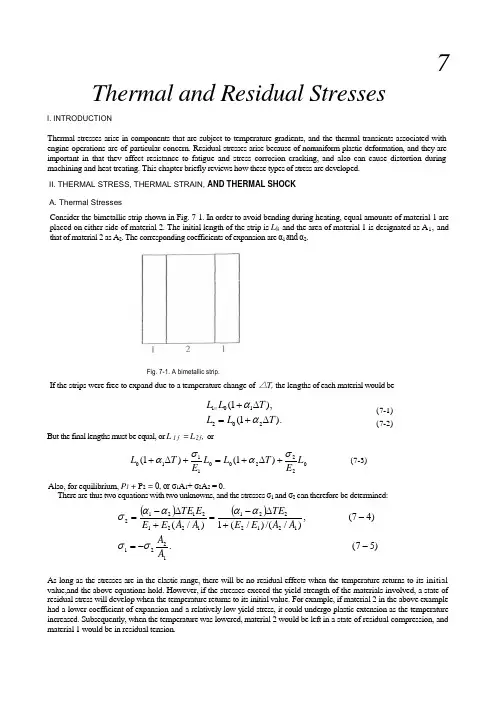
7Thermal and Residual StressesI. INTRODUCTION Thermal stresses arise in components that are subject to temperature gradients, and the thermal transients associated with engine operations are of particular concern. Residual stresses arise because of nonuniform plastic deformation, and they are important in that thev affect resistance to fatigue and stress corrosion cracking, and also can cause distortion during machining and heat treating. This chapter briefly reviews how these types of stress are developed. II. THERMAL STRESS, THERMAL STRAIN, AND THERMAL SHOCKA. Thermal Stresses Consider the bimetallic strip shown in Fig. 7-1. In order to avoid bending during heating, equal amounts of material 1 are placed on either side of material 2. The initial length of the strip is L 0, and the area of material 1 is designated as A 1, and that of material 2 as A 2. The corresponding coefficients of expansion are α1 and α2.Fig. 7-1. A bimetallic strip.If the strips were free to expand due to a temperature change of △T, the lengths of each material would be(7-1)(7-2)As long as the stresses are in the elastic range, there will be no residual effects when the temperature returns to its initial value,and the above equations hold. However, if the stresses exceed the yield strength of the materials involved, a state of residual stress will develop when the temperature returns to its initial value. For example, if material 2 in the above example had a lower coefficient of expansion and a relatively low yield stress, it could undergo plastic extension as the temperature increased. Subsequently, when the temperature was lowered, material 2 would be left in a state of residual compression, and material 1 would be in residual tension.).1(),1(202101T L L T L L ∆+=∆+=ααB. Thermal-Mechanical Cyclic StrainsTransient thermal strains of a cyclic nature can arise in jet engine components such as disks, blades, and vanes. Figure 7-2 is a simplified thermal-mechanical cycle for blades in a gas turbine (1). Under cruise conditions, the blades are at 600°C. When engine power is increased, the surface temperature rises to 1100°C in 105 seconds. Fig. 7-2a. Engine power is then returned to the cruise condition, and the temperature falls to 600°C in another 105 seconds. The rate of heating and cooling is 4.76 °C/sec. The total strain is the sum of the strain due to thermal expansion plus the strain due to the thermal stresses developed. The mechanical strain versus time plot, shown in Fig. 7-2b, includes both elastic and plastic strains. On heating, the outer surface initially goes into compressive strain, but then the strain reduces to zero as the interior of the blade heats up. On cooling, the reverse procedure occurs. Figure 7-2c shows the counterclockwise diamond cycle that is the thermal-mechanical hysteresis loop for this transient thermal history. The corresponding stress versus mechanical strain hysteresis loops for single crystals in the [001] and [111] orientations are shown in Fig. 7-3. It is noted that the mean stress for the cycle is close to zero.For the [001] orientation, plastic deformation (or viscoplastic deformation) is pro-nounced at a strain of —0.8. For the [111] orientation, plastic deformation begins at a strain of —0.25. Such thermal mechanical histories are complex, but they are also obviously important in assessing the fatigue life of such components.Fig. 7-2.Thermal-mechanical cycle, (a) Temperature versus time, (b) Strain versus time. (c) Thermal-mechanical hysteresis loop. (From Remy, 1. Reprinted from Low Cycle Fatigue and Elasto-Plastic Behaviour of Materials, edited by K.-T. Rie and P. D. Portella, pp. 119-130, Copyright 1998, with permission of Elsevier Science.)Fig. 7-3. Stress versus mechanical strain hysteresis loops for [001] and [111] thermal mechanical fatigue (TMF) single crystal specimens of AM1 superalloy using the cycle depicted in Fig. 7-2. Comparison between a viscoplastic model (solid line) and experiment (symbols). (After Remy, 1. Reprinted from Low Cycle Fatigue and Elastic-Plastic Behaviour of Materials, edited by K.-T. Rie and P. D. Portella, pp. 119-130. Copyright 1998. with permission of Elsevier Science.)C. Thermal ShockThermal shock denotes the rapid development of a steep temperature gradient and accompanying high stresses that can result in the fracture of brittle materials. It can occur either on heating or cooling. For example, the sudden shutdown of turbine engine can result in cracking of protective platinum-aluminide coatings due to the tensile stresses that develop as the surface cools and tries to shrink but is restrained by the interior.An example of thermal shock that occurs during heating is as follows. Consider a glass bowl whose thermal conductivity is low.1. A hot liquid is poured into the bowl.2. The inside surface of the wall tries to expand because of the sudden rise in temperature.3. A biaxial compressive stress develops on the inside surface because expansion of the is resisted by thesurounding, still cool, wall material.4. This compressive stress system sets up a balancing tensile stress system in the outer, still cool portion of thewall.5. Fracture can initiate in the outer region if the magnitude of the tensile stress developed is sufficient to nucleate a crack at a weak point.III. RESIDUAL STRESSES CAUSED BY NONUNIFORM PLASTIC DEFORMATIONResidual stresses arise because of a gradient in plastic deformation caused either by mechanical deformation or by a thermal gradient caused during cooling of a metal or alloy from a high temperature to a low temperature. The sign of the residual stress is always opposite in sign to the sign of the applied stress that gave rise to the residual stress. Residual stresses are important in fatigue and stress corrosion cracking where they can be either beneficial or detrimental. If residual stresses are present prior to heat treatment or machining, they can be detrimental because they can result in distortion (warping).A. An Example of Mechanically Induced Residual Stresses: Springback after Bending into the Plastic Range (2) In sheet bending, the width w is much greater than the thickness /, and width changes are negligible. Therefore, bending can be considered to be a plane-strain operation with εv = 0, εz = — εx . Let z be the distance measured from the mid-plane of the s heet in the thickness direction, and let r be the radius of curvature of the mid-plane. The value of e v varies linearly from — t/2r at the inside of the bend (z = —t/2) to zero at the mid-plane (z = 0), to +t/2r at the outside of the bend (z = t/2). Figure 7-4 shows the stress through the cross section. The principal of superposition is used to show that unloading can be considered to be the reverse of loading, so that for purely elastic bending there is no residual stress after unloading.Fig. 7-4. Strip bending, elastic strains.Next, assume that the material is elastic ideally plastic, that is, there is no strain hardening in the plastic range. If the tensile yield stress is Y, the flow stress in plane strain o-0 will be 1. 15 Y. Figure 7-5 shows the stress distribution throughout the sheet for fully plastic behavior. Except for an elastic core at mid-plane (which will be neglected), the entire section will be at a stress, σx = ±σ0.Fig. 7-5. Strip bending, plastic strains on loading, elastic on unloading.To calculate the bending moment M needed to create this fully plastic bend, note that dF x = σx w dz, and that dM = z dF x = z σx wdz. Therefore, the fully plastic bending moment is⎰⎰+--===2/2/2/020)67(42t t t x x t w zdz w zdz w M σσσ(Note that the elastic bending moment that is needed to have σx just equal to σ0 would be w σ0 (t 2/6), so that the fully plastic bending moment is 50% higher.)When the external moment is released, the internal moment must go to zero. As the material springs back elastically, the internal residual stress distribution must result in a zero bending moment. Since the unloading is elastic,)77(.1'2-∆=∆-=∆x x x E v E εεσM — △M= 0 after springback, and therefore equating M and △M givesOrThe resulting residual stress)117(.31'3''11''00000/-⎪⎭⎫ ⎝⎛-=⎪⎭⎫ ⎝⎛-=⎪⎭⎫ ⎝⎛--=∆-=∆-=t z tE z E r r E E xx x x σσσσεσσσσOn the outside surface, z = t/2, and the residual stress cr'x equals —σ0/2. On the inside surface, the residual stress is +σ0/2. The distribution of stresses is shown in Fig. 7-5.Note that the sign of the residual stress is opposite to the sign of the stress that caused it. Also, plastic deformation is required, but the plastic deformation must be nonuniform. There is no residual stress associated with a tensile bar that has been uniformly stretched into the plastic region. On the other hand, residual stresses will develop at notches, and so on, if the material at the base of the notch is strained into the plastic range while the surroundings remain elastic.An important state of residual stress is that formed at the tip of a growing fatigue crack due to an overload in plane specimens. During fatigue crack growth, if a 100% overload is applied, the fatigue crack will subsequently undergo a period of reduction in rate of crack growth as the crack penetrates the plastic zone created by the overload. This slowdown is related to an increased level of com-pressive residual stress brought about by the overload. This residual stress is largely a plane stress, surface regions, and is brought about by the lateral contraction of material at the surface that occurs in the overload plastic zone. In ductile materials, this lateral contraction leads to the formation of an obvious dimple immediately ahead of the crack tip. The compressive stress develops as the load is reduced from the overload level, and for now. because of the lateral contraction, there is more material in planes parallel to and just below the surface of the overload plastic zone than before the overload. As the crack grows through the overload zone, these residual stresses are released, giving rise to an increased level of crack closure in the wake of the crack tip (see Chapter 10), which results in a slowing down of the rate of fatigue crack propagation. The extent of the slowdown in crack rate is a function of the overload level and the thickness of the specimen, being much more pronounced in thin as compared to thick specimens. The reason for this difference is that, in thick specimens, plane-strain conditions prevail throughout most of the specimen's thickness, and the lateral contraction associated with plane stress is absent under plane-strain conditions. Hence, the level of enhanced residual compressive stress due to an overload is much less in thick specimens than in thin. Surface compressive residual stresses are beneficial in fatigue and in stress corrosion cracking. For this reason, they are often deliberately introduced, by shot-peening, for example. Any cracks that form are retarded in their growth rates, much as in the case of an overload.B. Case Study: Shaft of a Golf ClubAt a golf driving range in Connecticut the shafts (tapered hollow tubes) of the clubs were sometimes bent or otherwise damaged in use and had to be replaced. A supply of replacement shafts was kept in a storage shed, which was at times damp and humid. The shafts were made of a low-alloy steel that had been chrome plated, which protected the exterior of the shaft from corrosion. Whereas a new shaft is sealed to the club head as well as at the grip end. and thereby protected from corrosion on the inside of the shaft, the replacement shafts were not sealed, and as a result the interiors of these replacement shafts underwent corrosion over a period of time.A golfer was driving balls with a club whose shaft was a replacement. As he struck a ball, the shaft fractured, and the end he was holding struck him in the eye. Fortunately, the damage to his eye was not serious, and he recovered completely. Upon examination of the shaft it was noted that the fracture origin was at a small dent in the shaft that preexisted the accident. The fracture had initiated at this dent on the inside of the shaft. The fracture origin, shown in Fig. 7-6, was more planar and brittle in appearance than was the fracture away from the origin, shown in Fig. 7-7, which exhibited the dimples characteristic of ductile fracture. It was concluded that the fracture was due to hydrogen embrittlement,⎭⎝⎭⎝)97(,'1112'4320-⎪⎭⎫ ⎝⎛-=r r t wE t w σ)107(,'3'110-=⎪⎭⎫ ⎝⎛-tE r r σwhichwas associated with corrosion and the seemingly innocuous dent which, because of springback, resulted in a residual tensile stress on the inside of the shaft at the periphery of the dent. When the dent was formed, material on the inside near the periphery of the dent went into compression, and material near the center of the dent went into tension. Upon springback, the signs of the stresses were reversed, and a residual tensile stress was left on the inside surface at the periphery of the dent.Fig.7-6. Macroscopic view of the area of the fracture origin in a failed golf shaft. The rough area at bottom is the corroded inside surface of the shaft.(Reprinted from Material Characterization, Vol.26,A.J.McEvily and I. Le May,pp.253-268,Copyright 1991,with permission of Elsevier Science.)Fig.7-7. Macroscopic view of fracture surface awwy from fracture origin in failed golf shaft. (Reprinted from Material Characterization, Vol.26,A.J.McEvily and I. Le May,pp.253-268,Copyright 1991,with permission of Elsevier Science.)IV. RESIDUAL STRESSES DUE TO QUENCHING On cooling a metal part from an elevated temperature, residual stresses may be developed. For example, if a massive piece of copper is cooled rapidly, the surface layers will cool before the interior, thus setting up tensile strains and stresses in the surface that are counterbalanced by compressive stresses in the interior. At elevated temperatures, these tensile and compressive stresses are relaxed due to the low yield strength of the material. However, at a later point in the cooling process, the already cooled surface layer will be subjected to compression as the interior finally cools and shrinks. In general, the resultant compressive stress in the surface layers is beneficial, except when machining follows and distortion results from the nonuniform removal of the surface.When steel is quenched to form martensite at a low temperature, the transformation from austenite to martensite is associated with a volume expansion of the order of 1-3%. At the surface, this initially results in a compressive stress, as in the case of copper, but when the underlying layer finally cools and expands, the surface is put into tension. These tensile stresses can be reduced by using a steel of lower hardenability so that the interior does not got through a martensitic transformation, but instead transforms to bainite at a higher temperature.B. Quench CrackingIn a steel, there is always the possibility of immediate quench cracking, due to the level of tensile residual stresses developed when untempered martensite is formed. However, cold cracking (or delayed cracking) is the more probable event, and for this reason, alloy steel parts that have been quenched are quickly transferred to tempering furnances or salt baths in order to mnimize the time available for cold cracking to develop. If cracks develop on quenching into water and the part is then transferred to a salt bath for tempering, an explosive reaction can occur as the water trapped in the cracks transforms into steam. Therfore, personnel carrying out this operation need to wear protective face masks and protective clothing.It is also possible to develop quench cracks above the quench temperature if, during the quench of a material with low ductility, the tensile surface stresses that develop due to the temperture gradient in the material exceed the resistance to cracking of the material, as indicated in Fig. 7-8.Fig. 7-8. A schematic of thermal stress versus resistance to cracking as a function of temperature.To avoid the development of residual stresses, heat-treating procedures are used that minimize the temperature gradients responsible for the residual stresses. Such methods are:(a) Martempering: The steel is rapidly cooled to a temperature above the M s and held to allow a uniformtemperature to develop before further cooling to martensite.(b) Austempering: The steel is rapidly cooled to a temperature above the M s and held there until the transformation tobainite is complete before further slow cooling to room temperature.V. RESIDUAL STRESS TOUGHENINGIf the outer surface of the bowl discussed above in the section on thermal shock had been treated to have a residual compressive stress in the surface region, the resistance to thermal shock would have increased. Glass can be toughened by diffusing large atoms into the surface to develop residual compressive stresses on cooling as, for example, in Corningware. Tempered glass is created by cooling rapidly from an elevated temperature to develop compressive surface residual stresses, much as in the case of a block of copper. This type of glass is used in the side windows of automobiles. When such glass breaks, it fractures into many small fragments. However, the glass used in windshields is not tempered. A windshield consists of a sandwich of two sheets of glass between which is bonded a sheet of plastic. In a crash, the windshield is intended to be flexible enough to reduce head injuries, but be resistant enough to overall fracture to prevent front seat occupants from being ejected through the windshield. In this case the glass generally breaks into large shards that remain attached to the plastic membrane.VI. RESIDUAL STRESSES RESULTING FROM CARBURIZING, NITRIDING, AND INDUCTIONHARDENINGA. CarburizingCarburizing is carried out in the austenitic range and can lead to the development of a compressive residual stress at the surface in a low-alloy steel during quenching for the following reason (3, 4). Carbon is one of the elements that depresses the M s temperature of a steel. The M s temperature of the carburized surface layer, therefore, can be much lower than that of the interior because of the differential in carbon contents. On quenching, the interior, even though at a higher temperature than the surface, is the first to transform due to its higher M s temperature. Later on, the surface transforms and tries to expand but is now restrained by the already transformed interior. As a result, the surface is left in a state of residual compression, as indicated in Fig. 7-9.Fig. 7-9. Effect of carburization on the residual stresses in a quenched and tempered (1 hr at 180-200°C) 0.93 Cr-0.26 C steel (After Ebert, 3, and Krause, 4).B. NitridingNitriding is carried out at an elevated temperature below the eutectoid temperature for time periods of the order of 9-24 hours, and during the nitriding process any prior residual stresses are relaxed. The purpose of nitriding is to improve the surface wear and fatigue properties. Since the temperatures are lower than in carbur-izing and no phase transformation is involved, problems with distortion are minimized, an important consideration when heat treating carefully machined parts such as crankshafts. The formation of nitrides leads to a beneficial compressiveresidual stress in the surface even after the usual slow cooling because of a lower coefficient of expansion of the nitrides.C. Induction HardeningInduction hardenmg is a surface-hardening process in which only the surface layer ot a suitable ferrous workpiece is heated by electrical induction to above the transformation temperature and immediately quenched. Compressive residual stresses develop as the surface layers transform from austenite on quenching.VII. RESIDUAL STRESSES DEVELOPED IN WELDINGIn welding operations, the parts being joined often provide a large heat sink, and therefore cooling rates are rapid. As a result, untempered martensite may form in a residual tensile stress field and lead to weld cracking, either through cold cracking or quench cracking. The susceptibility to weld cracking increases as the number of unfavorable welding conditions increases. For example, a medium-carbon steel welded wuh an electrode not of the low-hydrogen type, and without preheat or postheat. may perform satisfactorily even though there may be a HAZ containing a region of martensite about 1/16 inch thick if joint restraint is low and cyclic loading m service is limited. However, if the section thickness is doubled, the level of residual stress rises due to greater constraint, and the thickness of the martensitic zone is increased due to a higher cooling rate, and cracking may develop. Even the use of low-hydrogen electrodes may not prevent cracking of the thicker section but the use ot a 315℃ (600°F) preheat will prevent cracking by retarding the rate of cooling, and thereby reducing the level of the residual stresses and the amount of marten-site formed.On cooling below the M s temperature, two forms of martensite can form depending upon carbon content. In low-carbon steels, the martensite is made up laths that contain a high density of dislocations. In higher carbon steel, the martensite is made up of plates that also contain a high dislocation content, but in addition may be twined. Preheating is used to reduce the cooling rate in order to minimize the likelihood of the formation of brittle martensite, particularly the twinned martensite. The preheat temperature increases with carbon content and with the thicknessOf the plates being welded, With recommended preheat temperatures ranging from 100°F for a 0.2 wt % C steel up to 600°F for a 0.6 wt % C steelPostweld heating of a weldment serves two purposes. One is to relieve the residual stresses that may have been developed during the welding process. The second is to temper both the weld deposit and HAZ to improve their fracture toughness. It is now mandatory that weldments in all nuclear components and in most pressure vessels be postweld heat treated (PWHT). These postweld heat treatments are carried out at a temperature of the order of 650°C (1200°F) for one hour.(a)Stresses parallel to weld (b)Stresses transverse to weldFig. 7-10. Transverse and longitudinal residual stresses developed at a butt weld. (From Gurney, 5. With permission of the Cambridge University Press.)The residual stresses that are developed both parallel to and transverse to a butt weld due to shrinkage of the weld metal on cooling are shown in Fig. 7-10 (5). To minimize distortion, weld passes were made from each edge of the plate toward the center, which accounts for the transverse residual stress distribution, since the last weld metal to solidify was in the central region of the butt weld. The residual stress developed during welding can sometimes be beneficial. For example, the fatigue strength of steel lap welded joints for automotive use was improved by using low transformation temperature (M.s200°C, M f20°C) welding wire (10Cr-10Ni), which induced compressive residual stresses in the surface layers. The fatigue strength at 108 cycles was increased from 300 MPa to 450 MPa by this procedure (6).VIII. MEASUREMENT OF RESIDUAL STRESSESThe two main methods for the determination of the magnitude of residual stress, the x-ray method and the metal removal method, were described in Chapter 5. Another example of the metal removal method is known as the boring-out method. This method can be used to determine residual stress levels in cannon or other cylindrical bodies. In the case of a cannon barrel, as a last step in the manufacturing process, a pressure is developed within the barrel of sufficient magnitude to expand the interior of the barrel into the plastic range. When the pressure is removed, a beneficial state of residual compressive stress is developed on the inner surface, a process known as autofrettage. The determination of the magnitude of the residual stresses by the boring-out method involves the machining away of successive layers from the interior of the barrel. As each layer is removed, some of the residual stress is relieved. As a result, on the outer surface of the barrel, longitudinal and cir-cumferential strains develop which are measured by strain gauges. From these measurements the magnitude of the initial residual stress state can be deduced.X. SUMMARYTHe thermal stresses that arise in engineered items, such as the turbine disks of jet aircraft engines, are no longer a major problem because of improvements in materials as well as better design procedures. Nevertheless, their presence must be taken into account. Problems with thermal cracking during heat treatment continue. Residual stresses are still a problem because their presence may not be recognized until a cracking problem associated with them develops.REFERENCES(1) L. Remy, in Low Cycle Fatigue and Elasto-Plastic Behavior of Materials, ed. by K.-T. Rie and D. P. Portella. Elsevier, Oxford. UK.1998, pp. 119-130.(2) W. F. Hosford and R. M. Caddell. Metal Forming, 2nd ed., Prentice-Hall, Engelwood Cliffs. NJ, 1993.(3) L. J. Ebert, The Role of Residual Stresses in the Mechanical Performance of Case Car-burized Steel. Met Trans. A. vol. 9A. 1978.pp. 1537-I551.(4) G. Krauss, Principles of Heat Treatment of Steel. ASM. Materials Park. OH, 1980.(5) T. R. Gurney, Fatigue of Welded Structures. Cambridge University Press, Cambridge, UK, 1968. p. 58.(6) A. Ohta, Y. Maeda. and N. Suzuki, in Proc. 25th Symp. on Fatigue, Japan Soc. Mats. Sci., 2000, pp. 284-287.。
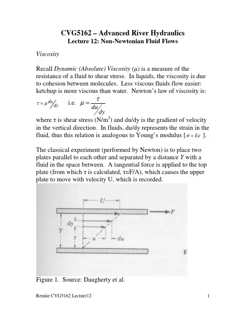
CVG5162 – Advanced River HydraulicsLecture 12: Non-Newtonian Fluid Flows Viscosity Recall Dynamic (Absolute) Viscosity ( ) is a measure of the resistance of a fluid to shear stress. In liquids, the viscosity is due to cohesion between molecules. Less viscous fluids flow easier: ketchup is more viscous than water. Newton’s law of viscosity is: dy duµτ= i.e. dydu τµ=where is shear stress (N/m 2) and du/dy is the gradient of velocity in the vertical direction. In fluids, du/dy represents the strain in the fluid, thus this relation is analogous to Young’s modulus [εσE = ]. The classical experiment (performed by Newton) is to place two plates parallel to each other and separated by a distance Y with a fluid in the space between. A tangential force is applied to the top plate (from which is calculated, =F/A), which causes the upper plate to move with velocity U, which is recorded. Figure 1. Source: Daugherty et al.With the no-slip assumption, the fluid particles next to each plate will assume the velocity of the plate. For laminar steady flow, the velocity gradient in the fluid between the plates will be linear.(i.e. du/dy is constant).Fluids for which does not depend on du/dy are described as Newtonian. Most common fluids are Newtonian. However, particularly relevant for some geophysical flows, fluids with very high suspended sediment concentration can be non-Newtonian. If one assumes that a fluid has zero viscosity (and therefore zero friction), the fluid is termed an ideal fluid. Note that an ideal fluid will not undergo strain due to the applied stress, thus it would maintain zero velocity between the two plates.Figure 2. Source: Daugherty et al.Viscosity of a fluid decreases with temperature, because cohesion diminishes. The dynamic viscosity of water at 20ºC is 1.005E-3 N s/m 2. Kinematic Viscosity ( ) is the dynamic viscosity divided by density: ρµν=. The kinematic viscosity of water at 20ºC is 1.007E-6 m 2/s. Turbulent eddy viscosity We have also seen that turbulence adds an extra apparent (eddy) viscosity (νT ), which is due to the increased transfer of momentum between fluid layers as a result of the turbulent motion (i.e. the Reynolds stress): ()dy du uv dy du T νννρτ+=−= Non-Newtonian Fluid We can see from Figure 2 above, that a Non-Newtonian fluid does not have a linear relation between shear stress and strain. In other words, the viscosity coefficient µ is not a constant – it varies with the shear stress applied. Some non-Newtonian fluids are relatively straight-forward, in that the instantaneous shear depends only on du/dy (as in the figure above). These are described as ‘time independent’, ‘purely viscous’, ‘inelastic’, or ‘generalized Newtonian fluids’ (GNF) (Chabbra and Richardson 1999, p.5). In more complex time-dependent non-Newtonian fluids the instantaneous apparent viscosity also depends on the flow history and previous shear rate.An important distinction between types of time-independent non-Newtonian fluids is whether or not they display a yield strength (i.e. whether a threshold stress is required to initiate strain (deformation) of the fluid, i.e. the stress required to get the fluid moving). See Figure 3. Note that the field of rheology bridges non-Newtonian fluids, plastic solids, and soils. Typically, the viscosity of a time-independent non-Newtonian fluid is specified as a function that depends on du/dy. Secondly, a yield stress term may be included. A viscoplastic is a fluid that displays a yield stress. A Bingham-plastic is a viscoplastic with a linear relation between shear and strain once yield shear is obtained:+=dy du y ηττ where τy is the yield stress (the stress required to initiate strain), and η is the dynamic viscosity (the slope of the line after the yield stress). A shear-thinning or pseudo-plastic fluid has no yield stress, but a relatively high viscosity at low strain. A shear-thickening or dilatant fluid has no yield stress, but a relatively low viscosity at low strain (high viscosity at high strain).Figure 3. Source: Chhabra and Richardson 1999. Note that pseudo-plastic fluid and shear-thinning fluid are synonomous. Figure 1.5 applies to polymer solutions, but shows how apparent viscosity decreases with increasing strain rate for a pseuodplastic fluid.Water-Sediment Mixtures The behaviour of fluids with high suspended sediment volumetric concentration (C s ) encompasses the range from Newtonian, to pseudo-plastic, to Bingham plastic, to yield-pseudoplastic depending on sediment concentration. Furthermore, individual clays have different electrochemical properties, and therefore different rheology. The analysis of high C s flows is thus complex. Julien and Lan (1991) provided a succinct summary of research until that time. Bagnold (1954) initiated this research field, and proposed that at high C s , fluid shear would be dominated by interparticle friction and collisions. He found that under very high rates of shear (i.e. high du/dy) and high C s , the shear stress increases as a second power of du/dy. Thus, the fluid can be described as a yield-pseudo plastic with convexivity to the shear stress (see Figure 4). The increased particle interactions at higher du/dy results in increased apparent viscosity (i.e. shear thickening). An empirical power-law equation (Herschel and Bulkley 1926) can be used for the shear in high clay-water suspensions at high du/dy (Govier and Aziz 1987, cited in O’Brien and Julien 1988):n y dy du a +=ττNote that n=2 based on the Bagnold observations. Alternatively, O’Brien and Julien (1988) found that under lower du/dy, the shear stress varies linearly with du/dy, thus at low du/dy the fluid mixture can be described as a Bingham plastic. They also argued that these are more realistic shear rates (du/dy) for geophysical flows. Note that both the yield stress and the dynamic viscosity increase exponentially with sediment concentration – three orders or magnitude increase between C s = 0.1 and 0.4 (O’Brien and Julien 1988)Julien and Lan provide the following summary plots: Figure 4. Source: Julien and Lan (1991)Figure 5. Source: Julien and Lan (1991)O’Brien and Julien (1985), cited in Julien and Lan (1991), proposed the following:2 ++=dy du dy du y ζηττwhere the first term is for the yield stress, the second for viscous (dynamic) stress, and the third term for the ‘turbulent-dispersive’ stress, which accounts for both turbulence and particle-particle interactions, both of which are presumed to vary as a second power with du/dy.Note that 2212s s d a l λρρζ+=, where ρ and l are mixture density and mixing length, a 1 is Bagnold’s empirical constant, λ varies with sediment concentration, and ρs and d s are sediment density and grain size. Note that the first term works out to be the turbulent Reynolds stress, and the second term is Bagnold’s stress due to particle interactions.Julien and Lan (1991) non-dimensionalized their model (see paper) to collapse the various data sets:Figure 6. Source: Julien and Lan (1991)TemperatureCoussot and Piau (1994) found little change in mud suspension rheological behaviour for temperatures ranging from 0°C to 20°C.Thixotropic Non-Newtonian FluidChanson (2006) presented a model for 1D dam-break flow of a high C s thixotropic fluid. A thixotropic fluid is a solid gel-like substance when at rest, but liquefies when agitated. The precise definition of thixotropy is a fluid which undergoes a decreasing apparent viscosity (i.e. reduced shear stress) when exposed to a constant rate of shear (i.e. du/dy) (Chhabra and Richardson 1999). Thus, viscosity is time-dependent. Mud suspensions tend to display thixotropy (Figure 7).Figure 7. Source: Chhabra and Richardson (1999)Chanson utilized a model by Coussot et al. (2002) for the viscosity of a thixotropic fluid:()n o a λµµ+×= whereλαθλ×∂∂×−=∂∂yV t 1 and the four terms µo , n, θ, and α are constants for a given fluid. Note that the viscosity in this model is time dependent. In general , numerical modelling of non-Newtonian fluids involves defining a relation that describes the viscosity of the fluid as a function of the fluid properties and flow (particularly du/dy). This equation must then be included in the set of equations to be solved. References Chanson, H., Jarny, S., and Coussot, P. (2006). "Dam break wave of thixotropic fluid." J. Hydraulic Eng., 132(3), 280-293. Chhabra, R., and Richardson, J. (1999). Non-Newtonian Flow in the Process Industries: Fundamentals and Engineering Applications , Butterworth Heinemann, Oxford. Daugherty, R. L., Franzini, J. B., and Finnemore, E. J. (1985). Fluid Mechanics with Engineering Applications, Eighth Edition , McGraw-Hill Book Company, New York. Julien, P. Y., and Lan, Y. (1991). "Rheology of hyperconcentrations." J. Hydraulic Eng., 117(3), 346-353. O'Brien, J., and Julien, P. (1988). "Laboratory analysis of mudflow properties." J. Hydraulic Eng., 114(8), 877-887.。

附录:常用专业词汇和用语汇总表Aabsolute temperature 绝对温度abutment [ə'bʌtmənt] n.桥墩;桥基;桥台acceleration [æk,selə'reɪʃən] n. 加速度accelerometer [æk,selə'rɔmitə] n.加速度计action-at-a-distance 远距离作用active gage 工作片acoustic emitter 声发射器acute angle 锐角adaptivity [ədæp'tivəti] n.适应性aerospace engineering 航空工程aggregate ['æɡriɡit] n.偏析,聚合体algebraic equation 代数方程Almansi strain 阿曼西应变allowable stress 许用应力alternator ['ɔ:ltəneitə] n. 交流发电机amorphous [ə'mɔ:fəs] adj.无定性的;非晶形的,无一定方向的amphiphile n.两亲物;两亲性分子amphiphile n.两亲物amplitude ['æmplitju:d] n.幅值amplification factor 放大因子,放大倍数amplitude stress 幅值应力amplitude of vibration 振动幅值;振幅anelastic [ˌænilˈæsti]adj.滞弹性的aneurysm ['ænjurizəm] n.动脉瘤anisotropic [æn,aisə'trɔpik] n.各项异性的297anisotropy [ænai'sɔtrəpi] n.各项异性apparatus [,æpə'reitəs] n.仪器;装置apparent stress 表观应力appearance [ə'pirəns] n.出现,显露,外观aqueous ['eikwiəs] adj. 水的;水成的arch [ɑ:tʃ] n.拱arm [ɑ:m]n. 臂artificial heart valve 人工心脏瓣膜assembly [ə'sembli] n. 组集,集合Atomic Force Microscope 原子力显微镜autocatalytic [,ɔ:təukætə'litik]adj.自动催化的austenite ['ɔ:stə,nait]n.奥氏体austenite crystal 奥氏体晶粒austenitic transformation 奥氏体转变average stress 平均应力axil force 轴向力Bback difference 向后差分backing ['bækiŋ]n.衬底;基底bar [bɑ:] n.杆;条;横木;栅basalt [bə'sɔ:lt] n. 玄武岩basis function 基函数Bauschinger effect 包辛格效应beam [bi:m] n. 梁,桁,横梁bedding plane 层理面benchmark test 基准测试bend [bɛnd] vt.&vi. 弯曲,折弯298bending moment 弯矩bending stress 弯曲应力biaxial strain 双轴应变biaxial stress 双轴应力biharmonic [baihɑ:'mɔnik]adj. 双调和的bionanomaterial n.生物纳米材料block copolymer 嵌段共聚物bobbin ['bɔbin] n.线轴body force 体力bolt [bəult]n.螺栓bomb blast 炸弹爆炸borehole ['bɔ:,houl] n.钻孔boron ['bɔ:rɔn] n.硼boundary condition 边界条件boundary integral 边界积分brake drum 制动鼓;鼓式制动器brass [brɑ:s] n. 黄铜,黄铜色brittle fracture 脆性断裂brittle fracture mechanics 脆性断裂力学buckle ['bʌkl] vi. 屈曲bushing ['buʃiŋ]n.绝缘套,轴衬Ccalcite ['kælsait]n.方解石calibration [,kæli'breiʃən] n.标定calibration constant 标定常数cantilever ['kæntili:və] n. 悬臂;支架carbon steel 碳钢Cartesian coordinate 笛卡儿坐标299cast iron 铸铁catastrophically [,kætə'strɔfikli] adv. 灾难性地cavitation [,kævi'teiʃən] n.气穴;成洞cellular pattern 空泡centered difference 中心差分central crack 中心裂纹centripetal acceleration 向心加速度centroidal axis 形心轴,质心轴chaotic [kei'ɔtik] adj.混乱的;混沌的chord [kɔ:d] n.弦;弦杆civil engineering 土木工程cleavage ['kli:vidʒ] n.分裂;裂隙clay soil settle 粘土土层沉降closed form 闭型cluster ['klʌstə] n.群;群集civil engineering 土木工程coarse-grain 粗粒的;大粒度的collapse [kə'læps] vi.破坏,塌陷collinear [kɔ'linjə] adj. 同线的;共轴的collision [kə'liʒən] n. 相撞,碰撞colloid ['kɔlɔid] n.胶体adj.胶状的column ['kɔləm] n. 柱体,圆柱columnar jointing 柱状节理combustion [kəm'bʌstʃən] n.燃烧,氧化complex frequency response 复频响应compliance [kəm'plaiəns] n.柔度composite material 复合材料300compressibility 可压缩性compressive stress 压应力computational mechanics 计算力学concomitant [kən'kɔmitənt] adj.伴随的;共存的concrete ['kɔnkri:t] n.混凝土,凝结物conservation of momentum 动量守恒consistency [kən'sistənsi] n.收敛性constraint [kən'streint] n. 约束contaminant [kən'tæmənənt]n.杂质;污染物continuum mechanics 连续介质力学contractile [kən'træktail] adj.可压缩的contracted notation 缩约记号contour ['kɔntuə] n.轮廓,等高线convection-diffusion 对流扩散convective velocity 对流速度convergence [kən'və:dʒəns] n.收敛convergence rate 收敛速度coolant ['ku:lənt] n.冷冻剂Coriolis acceleration 科氏加速度corrosion [kə'rəuʒən] n. 腐蚀,侵入corrosion resistance 耐蚀性;抗腐蚀性couple-stress 偶应力couple ['kʌpl] n. 力偶vt.偶合curvature ['kə:vətʃə] n.弯曲;曲率corrugate ['kɔrugeit] vt. &vi. 起皱纹complex truss 复式桁架compound truss 复氏桁架301criterion [krai'tiəriən] n.标准;准则coplanar [kəu'pleinə] adj. 共平面的concurrent [kən'kʌrənt] adj.同时发生的configuration [kən,figju'reiʃən] n.构型,结构,形态critical form 危形complementary function 余函数critical damping 临界阻尼conjugate ['kɔndʒə,geɪt] adj.共轭的constituent [kən'stitjuənt] adj.本质的,本构的constitutive theory 本构理论constitutive equation 本构方程constantan ['kɔnstəntæn]n.一种铜与镍的合金contrived variational principle 约束变分原理corrosion fatigue 腐蚀疲劳counter stress 对应力;相反应力crack [kræk] vt.&vi裂开,爆裂,断裂n.裂纹crack front 裂纹前沿crack initiation 裂纹起始;起裂crack nucleation 裂纹成核crack propagation 裂纹扩展crack tip 裂尖creep [kri:p]vi. 蠕变n.蠕变creep fatigue 蠕变疲劳creep fracture 蠕变断裂cross-bracing 交叉撑条cross joint 横节理302cross section 横截面critical state 临界状态critical load 临界载荷crook [kruk] vi.弯曲,成钩状crookedness ['krukidnis] n.弯曲;扭曲crush [krʌʃ] vt.&vi 压碎;折皱crystal lattice 晶格cull [kʌl] vt. 剔除n. 剔除culminate ['kʌlmineit] vi.达到顶点cycle number 循环次数cyclic loading 循环载荷cyclic stress 循环应力cylinder head 汽缸盖Ddamage ['dæmidʒ] n.损伤vt 损坏damping ['dæmpiŋ]adj.阻尼damping factor 阻尼系数dashe line 虚线dead weight 静止重量;自重;净重dealloying [,di:ə'lɔiiŋ]n.脱合金成分腐蚀decameter ['dekə,mi:tə] n. 十米defect [di'fekt]n.缺陷deflect [di'flekt] vt.&vi.偏斜,转向deflection [di'flekʃən] n.挠曲,挠度,偏斜deform [di'fɔ:m] vt.&vi.变形deformation [,di:fɔ:'meiʃən] n.变形degree of freedom 自由度303degree of redundancy 冗余度denominator [dɪ'nɔmə,neɪtə] n.分母density functional theory (DFT) 密度泛函理论derivative [di'rivətiv] n. 导数determinate [di'tə:minit] adj.确定的,静定的determinate structure 静定结构deviatoric plane 偏平面deviatoric stress 偏应力die [dai] n.冲模, 钢模die-cast housing 压铸壳differential equation 微分方程differentiation [,difə,renʃi'eiʃən]n.微分differential operator 微分算符diffusion coefficient 扩散系数digital image correlation 数字图像相关dimensionless [də'menʃənləs] adj.无量纲dip [dip] n. 浸泡;浸;下沉;倾斜vt.&vi.浸泡;浸;下沉;倾斜dip coating 浸涂Dirac delta function 狄拉克δ函数direction cosine 方向余弦Dirichlet condition 狄利克来条件discipline ['disiplin, 'disəplin] n.学科discrete 离散的dislocation [,dislə'keiʃən] n.位错displacement [dis'pleismənt] n. 位移displacement function 位移函数dissipation principle 耗散定理304divergence [dai'və:dʒəns] n.散度,分歧,分离dolerite ['dɔlərait] n.辉绿岩,粗粒玄武岩dolomite ['dɔləmait] n.白云石,石灰石drag [dræg] n.阻力droplet ['drɔplit] n.小滴;微滴ductile ['dʌktail] adj.韧性的,柔软的ductility [dʌk'tiliti] n.韧性Duhamel's integral 杜哈美积分dummy resistor 假电阻;仿真电阻duty cycle 负载循环;工作周期dyke [daik] n.沟;渠;堤坝dynamics [dai'næmiks] n. 动力学;力学;动态dynamic crack growth 动态裂纹扩展Eearth-moving 运土的eccentricity [,eksen'trisiti] n. 离心;偏心率elastic [i'læstik] adj.弹性的elastic limit 弹性极限elastic-perfectly plastic 理想弹塑性elastic-plastic 弹塑性的elastic wave 弹性波elasticity [,elæs'tisəti] n.弹性elasticity matrix 弹性矩阵elastomer [i'læstəmə] n.弹性体elastoplastic [i'læstəplæstik] n.弹塑性elasto-viscoplastic 弹粘塑性的electrical resistance strain gage 电阻应变计element ['elimənt] n.构件,要素,成分305elongate ['i:lɔŋgeit]vt. & vi.拉长;伸长;延长elongation [,i:lɔŋ'geiʃən] n.伸长,延长embossing [im'bɔ:s] vt.压纹;模压加工emulsion [i'mʌlʃən] n.乳胶液;感光乳剂encapsulation [in,kæpsju'leiʃən] n.包装;封装energy release rate 能量释放率engine block 发动机缸体engineering shear strain 工程剪应变epoxy [ep'ɔksi] n.环氧树脂equation of continuity 连续性方程equation of state 状态方程equilibrium [,i:kwi'libriəm] n. 平衡,均衡equilibrium equation 平衡方程equivalent nodal force 等效节点力error estimation 误差估计esthetics [es'θetiks] n.美学etch [etʃ] vt. 蚀刻ethanol ['eθə.nɔl, 'eθə.nəul] n. 乙醇Euler-Lagrange equation 欧拉-拉格朗日方程excavation [,ekskə'veiʃən] n.挖掘;发掘excitation [ek'saitətiv] n. 激励exigency [ek'sidʒənsi] n.紧急experimental stress analysis 实验应力分析explicit algorithm 显式算法extensometer [,eksten'sɔmitə] n.伸长计;引伸计external force 外力externally statically determinate 外部静定extreme position 极端位置306Ffailure ['feiljə] n. 破坏,失效fallacious [fə'leiʃəs] adj.谬误的;不合理的fashion ['fæʃən] vt.制造,使成形n.时尚fatigue [fə'ti:g] n.疲劳vi.&vt.(使)疲劳fatigue curve 疲劳曲线fatigue failure 疲劳破坏fault [fɔ:lt] n.断层felt pad 毛毡坐垫ferroelectric [,ferəui'lektrik]adj.铁电的fiber reinforced composite 纤维增强复合材料fibrous ['faibrəs] adj.纤维的finite element 有限单元finite difference method 有限差分法fixed-end 固定端flange [flændʒ] n. 凸缘;边缘;轮缘flexible ['fleksəbl] a dj. 柔度的,可弯曲的,柔韧的flexure ['flekʃə] n. 弯曲,曲率,挠度flow [fləu] vi.流动fluidics ['flu:idiks] n.应用流体学;射流技术fluid coupling 液力联轴节fluid mechanics 流体力学flux [flʌks] n.流量;熔化foil strain gauge 箔氏应变计folded plate 褶皱板force [fɔ:s] n. 力; 力量307forced vibration 强迫振动formula ['fɔ:mjulə] n. 公式formulate ['fɔ:mjuleit] vt.公式化,用公式描述forward difference 向前差分fracture ['fræktʃə] n.断裂vi.&vt. (使)断裂fracture mechanics 断裂力学fracture toughness 断裂韧性frame [freim] n.框架free-cutting alloy 易切削合金free vibration 自由振动frequency of vibration 振动频率friction force 摩擦力fringe [frindʒ] n.条纹fragment ['frægmənt]n.碎片;破碎functional ['fʌŋkʃənəl] n.泛函Ggage factor 应变灵敏度系数gas turbine engine 汽轮机geology [dʒi'ɔlədʒi] n.地质学,地质情况gigahertz [ˈɡiɡəhə:ts]n.十亿赫兹, 千兆赫gradient ['greidiənt] n.梯度,倾斜度grain [grein] n.晶粒granite ['grænit] n.花岗岩,花岗石graphite ['græfait] n.石墨grid [grid] n.格子Griffith‘s problem Griffith 问题gusset ['gʌsit] n. 角板;三角形衬料308gust [gʌst] n.阵风Hhanger ['hæŋə] n. 挂钩, 悬挂物hardening characteristic 硬化特性hardening rule 强化准则,强化定律hardness ['hɑ:dnis]n. 硬度,硬性harmonic [hɑ:'mɔnik]adj.简谐的harmonic force 谐力harmonic motion 简谐振动harness ['hɑ:nis]n.马具;管理;控制headway ['hedwei] n.前进;航行速度heat conduction equation 热传导方程heterodyning ['hetərəu,dainiŋ] n.外差作用heterogeneity [,hetərodʒi'ni:iti] n.非均匀性heterostructure [hetərəu'strʌktʃə(r)] n.异质结构heuristic [hjuə'ristik] adj.启发式的;探索的hierarchical [,haiə'rɑ:kikl]adj.按等级划分的hierarchical organization 分层结构high-cycle fatigue 高周疲劳high-frequency component 高频分量high-strength 高强度holder ['həuldə] n.固定器;支架holography [həu'lɔgrəfi] n.全息照相技术holy grail 圣杯;圣盘homogeneous [,homə'dʒinɪəs] adj. 同质的, 均匀的, 齐次的n.谐波homogeneous equation 其次方程Hooke's law 胡克定律309hostile environment 恶劣环境hydrodynamics ['haidrəudai'næmiks]n. 水动力学hydrostatic pressure 静水压力hysteresis [,histə'ri:sis] n.滞后(现象),滞后作用hysteresis loop 迟滞环;滞后回线Iideal gas 理想气体identity matrix 单位矩阵igneous ['igniəs] adj.火成的;火的imaginary part 虚部imaging method 成像法implicit algorithm 隐式算法impregnate [im'pregneit] vt.注入,使充满;adj. 充满的impress [im'pres] n.印象;特征;传送vi.印象;传送impulse-response function 脉冲响应函数inasmuch [inəz'mʌtʃ] adv. 由于;因为incompressible fluid 不可压缩流体indeterminate [,indi'tə:minit] adj.不确定的, 超静定的indeterminate structure 超静定结构indiscriminately [indi'skriminitli] adv. 无差别;任意地inertia [in'ə:ʃiə, in'ə:ʃə] n.惯性infinitesimal [,infini'tesiməl] adj.无限小的initial displacement 初始位移initial residual stress 初始残余应力initial velocity 初始速度initial yield surface 初始屈服面inorganic ['inɔ:'gænik] adj.无机的;非自然生长的310in-plane 面内I-shaped steel 工字钢instability [,instə'biliti] n. 不稳定insulating backing 绝缘基integral ['intigrəl] n. 积分;整数integral equation 积分方程integration [,inti'greiʃən] n.积分interferometry [,ɪntəfə'rɔmɪtə] n.干涉测量法interior cycle 内循环internal force 内力internal variable 内变量internally statically indeterminaten 内部静定interpolation function 插值函数interdisciplinary [,intə:'disiplinəri] adj. 学科间的;学科交叉的invariant [in'vɛəriənt] n.不变量; adj. 无变化的,不变的irreducible formulation 不可约型公式isothermal ['aisəu'θə:məl] adj.等温的n.等温线isotropic [,aisə'trɔpik] adj.各向同性的isotropic hardening 各项同性强化isotropy [ai'sɔtrəpi] n.各向同性iterative ['itərətiv] adj.迭代的Jjaw [dʒɔː]n.虎钳jelly ['dʒeli] n.胶状物J integral J积分joint [dʒɔint] n.节理311Kkinematic hardening 运动强化kinematics [,kinə'mætiks] n.运动学;动力学kinetic energy 动能kinetic friction 动摩擦LLagrangian [lə'grɑ:ndʒiən]adj. 拉格朗日的Lagrange method 拉格朗日方法Lagrange multiplier 拉格朗日乘子Lame constants 拉梅常数lamina ['læmənə]n.薄板;薄片laminar ['læminə] adj.层流laminate ['læmineit] n. 薄板;层压板;层板lamination [,læmi'neiʃən] n.制成薄板;薄板;层状体landslide ['lændslaid] n. 滑坡Laplace operator 拉普拉斯算符large-scale parallel computing 大规模并行计算lateral force 横向力lattice ['lætis] n.格子;点阵layer ['leiə] n.层least energy dissipation principle 最小能量耗散原理lifetime ['laiftaim] n.寿命linear elastic fracture mechanics 线性弹性断裂力学linear interpolation 线性插值linearized theory 线性化理论lipid ['lipid] n.脂质;油脂liquid crystal 液晶lithological [ li'θɔlədʒikəl ] adj.岩性的,岩石的312Lode parameter Lode参数longevity [lɔn'dʒeviti] n.长寿;寿命longitudinal ['lɔndʒi'tju:dinəl] adj. 纵向的,经度的longitudinal shear (or antiplane) mode of cracking 裂纹纵向剪切(反对称)模式longitudinal strain 纵向应变low-carbon steel 低碳钢low-cycle fatigue 低周疲劳lowly ['ləuli] adj.贫贱的;地位低下的Mmachinability [məʃi:nə'biliti] n.可切削性;机械加工性macro-mechanics 宏观力学macroscopic crack 宏观裂纹magnetic dot 磁点magnesium ['mæg'ni:ʃiəm] n. 镁mandrel ['mændrəl] n.心轴;拉延martensite ['mɑ:tən,zait] n.马氏体martensitic transformation 马氏体转变masonry ['meisnri] n.石造建筑;石造工程mass-spring-damper system 质量-弹簧-阻尼系统material derivative 物质导数mathematical statement 数学表达式,数学描述matrix ['meitriks] n.矩阵;基体(材料)matrices [复数] ['meitrisi:z]mean free path 平均自由程measurable ['meʒərəbəl] adj.可测量的mechanics [mi'kæniks] n. 力学mechanics of fluids 流体力学313mechanistic [,mekə'nistik] adj. 机械学的;机械的member ['membə] n. 构件meso-mechanics 细观力学mesostructure n.细观结构;中构造metallurgical [,metə'lə:dʒikl] adj. 冶金的metal forming 金属成型metamorphic [,metə'mɔ:fik]adj.变性的;变质的method of weigted residual 加权残值法micelle [mai'sel] n.微团;胶束microcavitation n.微空隙microcrack ['maikrəukræk, 'maikrəu.kræk] n. 微裂纹micro-electro-mechanical 微机电的micro-mechanics 微观力学microscopic ['maikrə'skɔpik] adj. 显微的,微观的microvoid [,maikrəu'vɔid] n.微孔military engineering 军事工程学mining ['mainiŋ] n.采矿;矿业mis-folding 错折叠mixed formulation 混合型公式mnemonic [ni:'mɔnik] adj.记忆的n. 记忆方法modal analysis 模态分析modality [məu'dæliti] n.样式;形式;形态modulus ['mɔdjuləs];n. 模量,系数moduli [复数] ['mɔdʒə,lai]modulus of elasticity 弹性模量modulus of volume expansion 体积膨胀模量Mohr-Coulomb failure criterion 摩尔-哥伦布破坏准则314moire [mwɑ:] n.云纹moire interferometry 云纹干涉法molecular dynamics (MD) 分子动力学moment of inertia 惯性矩momentum [məu'mentəm] n.动量,冲量monolithic [,mɔnə'liθik]adj. 独石的;单体的;整体的monotonic [mɔnəu'tɔnik] adj. 单调的;单斜晶体的Monte Carlo (MC) 蒙特卡罗mount [maunt] vt. 安装mud [mʌd] n.泥;泥浆Multi Body Dynamics (MBD) 多体动力学multiphase flow多相流multiplier ['mʌltəplaiə] n. 乘数multi-scale 多尺度myriad ['miriəd] n.无数;极大数量adj. 无数的;极大数量的Nnanocomposite n.纳米复合材料nanofabrication n.纳米加工nanohole n.纳米空洞nano-mechanics 纳米力学nanoscale n.纳米尺度nanostructure n.纳米结构nanowire n.纳米线natural frequency 固有频率natural variational principle 自然变分原理Navier‘s equation纳维方程necessary condition 必要条件315necking zone 紧缩区域Neumann condition 纽曼条件neutral axis 中性轴Newtonian fluid 牛顿流体Newton's first law 牛顿第一定律Newton's second law 牛顿第二定律nitrocellulose ['naitrəu'seljuləus] n.硝化纤维素nodal displacement 节点位移nondimensional ['nɔndi'menʃənəl] n. 无量纲adj.无量纲(的)nonhomogeneous ['nɔnhɔmə'dʒi:njəs] adj.非均质的;非齐次的;多相的nonlinearity [,nɔnlini'æriti] n.非线性normal force 法向力notwithstand [,nɔtwiθ'stændiŋ]prep.尽管;虽然numerator ['nu:mə,reɪtə, 'nju:-] n.分子non-cyclic load 非循环载荷nonhomogeneous ['nɔnhɔmə'dʒi:njəs] adj.非均匀的nonstationary ['nɔn'steiʃənəri] adj.不稳定的;非定常的nondestructive evaluation 无损评价nonviscous adj.非粘性,无粘性non-Newtonian fluid 非牛顿流体Oobjective function 目标函数oblique [əb'li:k] adj.斜的;倾斜offshore structure 离岸结构off-lattice 非格子off-road 越野的opening mode of cracking 裂纹张开模式316operator ['ɔpə,reitə] n.算符optimization [,ɔptimai'zeiʃən] n.优化optimize ['ɔptimaiz] vt.&vi.优化optimum ['ɔptiməm] adj. 最优的ordinary integral 寻常积分ordinary differential equation 常微分方程organic [ɔ:'gænik] adj. 有机的;有机物质orthotropic [,ɔ:θə'trɔpik] adj. 正交的oscillation [,ɔsi'leiʃən] n.振荡ostensibly [ɔs'tensəbli]adv.表面上地;外表上地out-of-plane n. 面外out-of-plane 面外outperform [,autpə'fɔ:m] vt. 优于;超额完成overstress ['əuvə'stres, .əuvə'stres] n. 过应力oxidize ['ɔksi,daiz] vt.& vi.(使)氧化Pparadigm ['pærədaim] n.范例partial differential equation 偏微分方程particular integral 特积分;特解particulate [pə'tikjulit] adj.微粒的particulate-reinforced composite 颗粒增强复合材料pendulum ['pendjuləm] n. 单摆,摆锤period of vibration 振动周期permanent deformation 永久变形perseverance [,pə:si'viərəns] n.不屈不挠;毅力phase [feiz] n.相phase angle 相位角317phenolics [fi'nɔliks] n.酚醛树脂photoelastic [fəutəui'læstik] adj.光弹性的photoelastic coating 光弹性涂层photoelastic stress analysis 光弹性应力分析piezoelectric [pai,i:zəui'lektrik] adj.压电的pile [pail] n.柱,桩,堆pinned end 销轴支承pin joint 铰接;关节接头piston ['pistən] n. 活塞pitch [pitʃ] n.沥青pixelate vt.使...像素化;将...分解成像素plane-strain 平面应变plane stress 平面应力plastic ['plæstik] adj.塑性的plastic flow塑性流动plastic wave 塑性波plasticity [plæs'tisiti] n.塑性ploughman ['plaumən] n.庄稼汉pneumatic [nju:'mætik] adj. 气动的;充气的Poisson effect 伯松效应Poisson‘s ratio泊松比polar coordinate 极坐标polarize ['pəulə,raiz] vi.&vt. (使)极化polycrystalline [pɔli'kristəlain] n.多晶体polymer ['pɔlimə] n.聚合物post [pəust] n.柱posteriori error estimation 后验误差估计potential energy 势能318predate [pri:'deit] vt.在日期上早于prestrain [pri:'strein] n.预应变primary structure 主要结构primary unknowns 主要未知量principal material axis 材料主轴principal stress 主应力printed circuit technique 印刷电路技术product 乘积proliferation [prə,lifə'reiʃən] n.增殖;扩散proportional limit 比例极限protein folding 蛋白质折叠pseudo-stochastic 伪随机的pulsating load 脉动载荷pulse excitation 脉冲激励pump [pʌmp] n.泵punch [pʌntʃ] vt. 钻孔pure shear 纯剪切Qquadratic [kwə'drætik] adj.二次的quadratic functional 二次泛函quantum mechanics 量子力学quasi-static 准静态,拟静态Rrate-dependednt 率相关的rate of dilation 膨胀率Rayleigh wave 瑞利波reaction [ri'ækʃən] n.支反力319reactor piping 反应堆管道red blood cell 红血球redundant constraint 多余约束reference axis 参考坐标系reinforced concrete 增强混泥土,钢筋混凝土reliability [ri,laiə'biliti] n.可靠性,可靠度reloading [ri:'ləudiŋ]vt. & vi.重复加载rendition [ren'diʃən] n.解释;演奏;投降repertoire ['repətwɑ:]n.全部节目;全部技能Representative Volume Element (RVE) 代表性体积单元reservoir ['rezəvwɑ:] n.蓄水库residual thermal stress 残余热应力resinous ['rezinəs]adj. 树脂的resin-coated adj. 树脂涂层的resonance ['rezənənt] adj. 共振response [ri'spɔns] n.响应,反应,回答resultant [ri'zʌltənt] adj.合成的,组合的resultant momentum 合力矩retool [ri:'tu:l] vi. & vt.重组;重新装备reversible [ri'və:səbl] adj.可逆的rib [rib] n.肋rigid-body 刚体rigid frame 刚架rigidity [ri'dʒiditi] n. 刚度,刚性rise time 上升时间rivet ['rivit] n.铆钉;铆接rock foundation 岩石基rock mechanics 岩石力学320rosette [rəu'zet] n.玫瑰花形物rotate [rəu'teit]vi.转动,旋转rotation [rəu'teiʃən]n.转动,旋转round-off error 舍入误差rubric ['ru:brik] n.类;标题;红色的Ssag [sæg] n.弧垂,垂度saturated soil 饱和土scalar ['skeilə] n. 数量;标量Scanning Electron Microscope (SEM) 扫描电子显微镜scanning mode 扫描方式Scanning Tunneling Microscope 扫描隧道电子显微镜second order derivative 二阶导数scouring ['skauəriŋ]n.擦洗;冲刷seed [si:d] vt. 崔云化雨sedimentary [,sedi'mentəri] adj.沉积的;沉淀性的;沉淀作用造成的seismic wave 地震波seismological [,saizmə'lɔdʒikl] adj.地震学上的seismology [saiz'mɔlədʒi] n.地震学sequel ['si:kwəl] n.结局;后果sewage ['sju:idʒ] n.污水,污秽物shadow moire 影栅云纹shape function 形状函数shape memory alloy (SM A) 形状记忆合金shape memory effect (SM E) 形状记忆效应shape optimization 形状优化shearing strain 剪切应变321shearing stress 剪切应力shock spectrum 冲击谱shock wave 冲击波;激波shrinkage 收缩;减少;损耗silicone gel 硅凝胶silly putty 弹性橡胶泥SI metric system 国际单位制simply supported beam 简支梁simple truss 简支桁架simultaneous [,saiməl'teinjəs] adj.同时发生的;同步的simultaneous equation 联立方程single-DOF 单自由度singularity [,siŋgju'læriti] n. 奇异性sintering ['sintəriŋ]vi.烧结sinusoidal function 正弦函数siting ['saitiŋ]n.建设地点sizing optimization 尺寸优化slab [slæb] n.平板;厚板slenderness ['slendənis] n.细长;细长度sliding ['slaidiŋ]n.滑移slip [slip] n.滑移slip plane 滑移面soil foundation 土基础soil mechanics 土力学solder ['sɔldə] n.焊接剂;接合剂solid mechanics 固体力学specified displacement 给定位移specified surface traction 给定面力322speckle interferometry 散斑干涉法spring constant 弹簧常数spring-supported 弹簧支撑stability [stə'biliti] n. 稳定,稳定性stainless steel 不锈钢statical indeterminancy 静不定static equilibrium 静力平衡static fatigue 静态疲劳static friction 静摩擦statics ['stætiks] n. 静力学stationarity [steiʃə'næriti] n.稳定性;稳态stationary ['steiʃənəri] adj.稳定的;不动的steady-state 稳态steel-framed 钢架step excitation 阶跃激励stereological [stiəri'ɔlədʒi, sterə'ɔlədʒi] adj. 体视学;立体测量学stereoscopic [,steriəs'kɔpik]adj.有立体感的stiffen ['stifn] vt.&vi. 刚化;使坚硬stiffness ['stifnis] n.刚度stocky ['stɔki] adj. 矮壮的;结实的strain [stren] n. 应变strain energy 应变能strain gage 应变计strain-induced quantum dot 应变诱发量子点strain rate 应变率strength [streŋθ] n.强度strength-to-weight ratio 比强度stress [strɛs] n. 应力323stress concentrator 应力集中点stress concentration 应力集中stress corrosion cracking 应力腐蚀起裂stress distribution 应力分布stress gradient 应力梯度stress-induced martensite (SIM) 应力诱发马氏体stress intensity factor 应力强度因子stress-matrix 应力矩阵stress ratio 应力比stress-strain diagram 应力应变图stress tensor 应力张量stress wave 应力波stretch [stretʃ] vt. & vi. 伸展,拉紧,.延伸strike [straik] vi.走向structural optimization 结构优化structural steel 结构钢sub-discipline 分支学科subdomain n.子域submicron ['sʌb'maikrɔn] n.亚微细米;亚微细粒adj. 表面活性剂的substrate ['sʌbstreit] n.基片;基底sufficient condition 充分条件super-hydrophobic 超蔬水superelasticity n.超弹性superposition [ˌsju:pəpəˈziʃən] n. 叠加,重叠,叠合support [sə'pɔ:t] n.支撑surface force 表面力surface traction 表面力324surfactant [sə:'fæktənt] n.表面活性剂symmetric [si'metrik] adj. 对称的Ttangent matrix 切线矩阵Taylor series expansion 泰勒级数展开T-beam T型梁tectonophysics [,tektənəu'fiziks] n.构造物理学, 地壳构造物理学tensile stress 拉应力tensile strength 拉伸强度tensile-testing machine 拉伸试验机tensile test specimen 拉伸试样tension ['tenʃən] n. 张量,张力,拉力tensor ['tensə] n. 张量tensor-transformation 张量转换theoretical and applied mechanics 理论与应用力学thermal camera 热感照相机thermal expansion coefficient 热膨胀系数thermal stress 热应力thermo-fatigue 热疲劳thermography [θə:'mɔgrəfi] n. 温度记录法;热熔印刷thermomechanics [θə:məumi'kæniks] n.热力学thermosetting resin 热固性树脂thrust [θrʌst] vt.&vi. 抛掷tillage ['tilidʒ] n.耕种,耕作time derivative 时间导数time lag 时间滞后titanium [tai'teiniəm] n. 钛325tolerating strain 容许应变tomographic [təu'mɔgrəfi] n.X线断层摄影术;X线体层照相术topography [tə'pɔgrəfi]n.地质,地形学topology optimization 拓扑优化trade-off n.权衡;取舍transducer [træns'dju:sə] n.传感器transient term 暂时项;衰减项transport equation 输运方程;迁移方程Transmission Electron Microscope (TEM) 透射电子显微镜transverse shear mode of cracking 裂纹横向剪切模式transversely isotropic 横观各向同性Tresca yield criterion 特雷斯加屈服准则trial and error 试错trial function 试函数triaxiality [traiæksi'æliti] n.三轴;三维triclinic [trai'klinik]adj.三斜晶系的true stress 真实应力truncation error 截断误差truss [trʌs] n.桁架turbulent flow湍流流动tunable ['tju:nəbl] adj.可调谐的turbulent ['tə:bjulənt] adj.湍流的twinned boundary 孪生边界two-span beam 双跨梁Uubiquitous [ju:'bikwitəs] adj.到处存在的ultimate tensile strength 最大拉伸强度ultrasonics [,ʌltrə'sɔniks] n.超声波, 超声学326unbalance ['ʌn'bæləns] n. 不平衡unconditionally stable 无条件稳定的undamped [ʌn'dæmpt] adj. 无阻尼的uniaxial strain 单轴应变uniaxial stress 单轴应力uniaxial tension 单轴拉伸unit impulse 单位脉冲unload ['ʌn'ləud] vt.& vt. 卸载upwind scheme 迎风格式Vvacuum deposition technique 真空淀积技术variable ['vɛəriəbl] n.变量adj.可变的variational principle 变分原理vector ['vektə] n. 矢量;向量vibration [vai'breiʃən] n.振动,震动vibratory ['vaibrətəri] adj.振动的Vierendeel truss 空腹桁架;弗伦第尔桁架virtual design 虚拟设计visco-elastic 粘弹性的viscoelastic wave 粘弹性波viscoelasticity ['viskəuilæs'tisiti] n.粘弹性visco-plastic 粘塑性的viscoplastic potential 粘塑性势viscosity [vis'kɔsiti] n.粘性viscosity coefficient 粘性系数viscous ['viskəs] adj. 粘性的viscous damping 粘性阻尼327von Mises yield criterion 冯米赛斯屈服准则volume fraction 体积分数volumetric strain 体积应变Wwavenumber n.波数wear resistance 耐磨性,耐磨度web [web] n. 腹板weld [weld] vt.&vi. 焊接n. 焊接weldability [weldə'biliti] n. 焊接性;可焊性Wheatstone bridge 惠斯通电桥whisker ['hwiskə] n.金须wire strain gauge 金属丝应变计work [wə:k] n. 功workability [,wə:kə'biliti] n.可使用性;施工性能;可加工性woven fiber 编织纤维wraparound ['ræpə,raund] adj.围绕的;围绕物wrought [rɔ:t] adj.锻造的;加工的;精细的Yyield criterion 屈服准则yield function 屈服函数yield point 屈服点yield strength 屈服强度Zzinc [ziŋk] n.锌328。
eagre 涌潮earth 土earth atmosphere 地面大气earth attraction 地球引力earth axis 地轴earth gravity 地球重力earth lateral pressure 土的侧压力earth orbit 地球轨道earth pressure 土压力earth pressure at rest 静土压力earth revolution 地球公转earth rotation 地球自转earth tides 地球潮汐earthquake force 地震烈度earthquake intensity 地震烈度earthquake proof 抗震earthquake proof wall 抗地震壁earthquake response 地震响应earthquake response spectrum 地震应谱earthquake shock 地震冲击earthquake wave 地震波easy glide region 易滑移区ebb tide 落潮ebullition 沸腾eccentric 偏心的eccentric anomaly 偏近点角eccentric collision 偏心碰撞eccentric compression 偏心压缩eccentric load 偏心荷载eccentric motion 偏心运动eccentric tension 偏心拉伸eccentricity orientation 偏心定向echo box 回波谐振盒echo pulse 回波脉冲echo wave 回波eddy 涡旋eddy conductivity 涡莲导率eddy current loss 涡琉耗eddy currents 涡流湍流eddy diffusion 涡动扩散eddy diffusivity 涡俩散率eddy energy 湍淋eddy energy flow 涡能通量eddy energy flux 涡能通量eddy field 涡场eddy flow 湍流涡流eddy freedom 无旋涡性eddy friction 涡动摩擦eddy generation 涡廖成eddy heat conduction 湍寥传导eddy invariant 涡旋不变量eddy loss 涡琉耗eddy motion 涡了动eddy resistance 涡凌力eddy source 涡源eddy space 涡琳间eddy spectrum 湍磷eddy stress 湍力力eddy transport 涡龄送eddy viscosity 涡脸性eddying whirl 涡流edge condition 边缘条件edge crack 边缘裂缝edge damping 边缘阻尼edge diffraction 边缘衍射edge dislocation 刃状位错edge effect 边缘效应edge fracture 边缘裂缝edge of crack 裂缝边缘edge point 边点edge wave 边缘波edgewise meter 边缘读数式仪表eerasive resistance 抗磨性effective area 有效面积effective coefficient 有效系数effective crack length 有效裂隙长度effective cross section 有效横截面effective energetic efficiency 有效能量效率effective head 有效水头effective horsepower 有效马力effective incidence 有效迎角effective length 有效长度effective load 有效负载effective mass 有效质量effective porosity 有效孔隙度effective pressure 有效压力effective radius 有效半径effective range of instrument 仪颇有效量程effective section 有效断面effective sound pressure 有效声压effective stress 有效应力effective surface energy 有效表面能量effective temperature 有效温度effective turbulent diffusivity 有效湍俩散系数effective value 有效值effective velocity 有效速度effective wake 有效伴流effective wavelength 有效波长effective work 有效功efficiency 效率effluence 瘤effluent 瘤水efflux 瘤efflux velocity 喷临度efflux viscometer 射脸度计effort 酌力effuser 喷管effusion 喷出eigen frequency 本盏率eigenfunction 本寨数eigenmoment 固有矩eigenperiod 固有周期eigenrotation 本正转eigentemperature 本章度eigentensor 本张量eigenvalue 本盏eigenvalue of energy 能量本盏eigenvector 本崭量einstein approximation 爱因斯坦近似einstein formula 爱因斯坦公式einstein frequency 爱因斯坦频率ejection seat 弹射座椅ejector 喷射器ekman flow 埃克曼流ekman helix 埃克曼螺线ekman layer 埃克曼层ekman number 埃克曼数elastic 弹性的elastic after effect 弹性后效elastic anisotropy 弹性蛤异性elastic axis 弹性轴elastic base 弹性基础elastic bending 弹性弯曲elastic buckling 弹性压曲elastic center 弹性中心elastic coefficient 弹性系数elastic coefficient matrix 弹性系数矩阵elastic collision 弹性碰撞elastic compliance 弹性顺度elastic constants 弹性常数elastic curve 弹性曲线elastic deformation 弹性形变elastic design 弹性设计elastic dipole 弹性偶极子elastic distortional potential 弹性形变势elastic elongation 弹性伸长elastic energy 弹性能elastic energy density 弹性能量密度elastic equilibrium 弹性平衡elastic failure 弹性破坏elastic fatigue 弹性疲劳elastic fiber 弹性纤维elastic fluid 弹性铃elastic force 弹力elastic foundation 弹性基底elastic ground 弹性地面elastic hardness 弹性硬度elastic heat wave 热弹性波elastic hysteresis 弹性滞后elastic hysteresis loop 弹性滞后曲线elastic impact 弹性碰撞elastic kernel 弹性核elastic lag 弹性滞后elastic limit 弹性极限elastic limit for compression 压缩弹性极限elastic limit for tension 拉伸弹性极限elastic line 弹性线elastic load 弹性负荷elastic membrane 弹性膜elastic modulus 弹性模数elastic oscillation 弹性振荡elastic plastic 弹塑性的elastic plastic body 弹塑性体elastic plastic deformation 弹塑性形变elastic plastic equilibrium 弹塑性平衡elastic plastic fracture 弹塑性断裂elastic plastic strain 弹塑性形变elastic porous flow 弹性渗流elastic potential 弹性势elastic potential energy 弹性势能elastic range 弹性区域elastic rebound 弹性复元elastic recovery 弹性复元elastic region 弹性区域elastic relaxation 弹性弛豫elastic ring 弹性环elastic scattering 弹性散射elastic scattering cross section 弹性散射截面elastic scattering submatrix 弹性散射子矩阵elastic shell 弹性壳elastic sol 弹性溶胶elastic state 弹性状态elastic strain 弹性形变elastic strain energy 弹性应变能elastic stress 弹性应力elastic support 弹性支承elastic surface 弹性曲面elastic vibration 弹性振动elastic viscoplastic 弹性粘塑性的elastic viscoplastic analogy 弹性粘塑性比拟elastic wave 弹性波elastic wave in bar 杆中弹性波elastica 弹性线elastically supported beam 弹性支承梁elasticity 弹性elasto osmometry 弹性渗压测定法elasto plastic bending 弹塑性弯曲elasto plastic interface 弹塑性分界面elasto viscosity 弹粘性elasto viscous solid 弹粘性固体elastodynamics 弹性动力学elastohydrodynamics 弹性铃动力学elastokinetics 弹性动力学elastomechanics 弹性力学elastomer 弹性体elastometry 弹性测量法elastoplastic material 弹塑性材料elastoplastic range 弹塑性范围elastoplastic wave 弹塑性波elastostatics 弹性静力学elbow 肘管electric displacement 介电移electric knudsen number 电气克努森数electric wind 电风electrical analogy 电比拟electrical fluid dynamics 电铃动力学electro conducting fluid 导电铃electro magnetic flow meter 电磁量计electrogasdynamics 电气体动力学electrohydraulics 电动水力学electrohydrodynamics 电铃力学electromagnetic continuum mechanics 电磁连续介质力学electromagnetic gun 电磁炮electromagnetic pump 电磁泵electromagnetic stirring 电磁搅拌electromagnetofluid dynamics 电磁铃动力学electromechanical pickup 机电传感器electromotive force 电动势electron cyclotron frequency 电子回旋频率electron diffusion coefficient 电子扩散系数electron sound velocity 电子声速electronic current 电子流electrostatically suspended gyroscope 静电支承陀螺仪element 元件element matrix 单元矩阵element of construction 建筑部件element of turbulence 湍联element of vortex 涡元elementary displacement 单元变位elementary wave 元波elementary work 元功elevation of pressure 增压elevator 升降机elevon 升降副翼ellipsoid of elasticity 弹性椭球ellipsoid of inertia 惯量椭球ellipsoid of stress 应力椭球ellipsoidal wave function 椭球面波函数elliptic coordinates 椭圆坐标elliptic function 椭圆函数elliptic pendulum 椭圆摆elliptic vortex of kirchhoff 基尔霍夫椭圆涡旋elliptical loading 椭圆加载elliptical orbit 椭圆轨道elliptical oscillation 椭圆振荡elliptical velocity 椭圆速度elongation 伸长elongation percentage 延伸率elongation quadric 伸长二次曲面elongational flow 伸长怜elutriation 淘析embrittlement 脆化emersion time 现出时间emersion wave 出现波emission 放射emissivity 辐射系数emollescence 软化empennage 尾翼empty state 空态empty weight 无载重量emulsified liquid 乳化液encounter 碰撞end effector 末端执行器end face flux 正面通量end face leakage flux 正面漏泄通量end on observation 轴向观察end on structure 端接结构end point energy 端点能量end rib 端肋end support 端点支承end thrust 轴向推力endothermic 吸热的endothermic reaction 吸热反应endurance 持久性endurance bending strength 抗弯疲劳强度endurance bending test 弯曲疲劳试验endurance failure 疲劳断裂endurance limit 疲劳极限endurance strength 疲劳强度endurance test 疲劳试验endurance testing machine 疲劳试验机energy 能energy absorption build up factor 能量吸收累积因子energy approximation 能量近似energy balance 能量平衡energy build up factor 能量累积因子energy carrier 能量载体energy conservation 能量守恒energy conservation law 能量守恒定律energy constant 能量常数energy content 能含量energy decrement 能量减量energy density 能量密度energy density spectrum 能量密度谱energy deposition 能量沉积energy dispersion formula 能量分散公式energy distribution 能量分布energy efficiency 能量效率energy equation 能量方程energy equivalent 能量当量energy exchange 能量交换energy exchange time 能量交换时间energy fault 能量缺陷energy flow 能通量energy flow density 能淋度energy fluence 能注量energy fluence build up factor 能注量累积因子energy flux 能通量energy flux density 能淋度energy flux of radiation 辐射能流energy function 能量函数energy generation 能量产生energy group 能量组energy head 能量头energy level density 能级密度energy line 能量线energy loss 能量损耗energy metabolism 能量代谢energy migration 能量迂移energy momentum flux 能量动量通量energy momentum tensor 能量动量张量energy of absorption 吸收能energy of attachment 附着能energy of combustion 燃烧能energy of interaction 相互酌能energy of thermal motion 热运动能量energy of turbulence 湍淋energy of vibration 振动能量energy operator 能量算符energy oscillation 能量振荡energy output 能量输出energy principle 能量原理energy relaxation 能量弛豫energy resolution 能量分辨率energy source 能源energy spectrum 能谱energy spectrum equation of turbulence 湍淋谱方程energy surface 能面energy transfer 能量传输energy unit 能单位engine power 发动机功率engine speed 发动机转速engineering fluid mechanics 工程铃力学engineering system of units 工程单位制engineering unit 工程单位engler degree 恶勒度engler viscosimeter 断粘度计enlargement 放大enlargement of pipe 管扩张enlargement scale 放大标度enrichment 浓缩entering 入射enthalpy 焓enthalpy of combustion 燃烧焓enthalpy of mixing 混合焓entrainment 卷入entrance loss 进口损失entrance pressure 进口压力entrance velocity 进口速度entropic efficiency 熵效率entropic wave 熵波entropy 熵entropy balance equation 熵平衡方程entropy elasticity 熵弹性entropy equation 熵方程entropy flow 熵流entropy increase 熵增加entropy inequality 熵不等式entropy layer 熵层entropy of evaporation 汽化熵entropy of formation 形成熵entropy of melting 熔融熵entropy of mixing 混合熵entropy wave 熵波envelope surface 包络面envelope velocity 包络速度environment 环境environment temperature 周围温度environmental aerodynamics 环境空气动力学environmental conditions 环境条件epicenter 震中epicycloidal motion 外摆线运动equal armed lever 等臂杠杆equal energy source 等能源equalization 均衡equalization of concentration 浓度均衡equalization of potential 位势均衡equally distributed 均匀分布的equating 均衡equation of compatibility 协到程equation of continuity 连续性原理equation of equilibrium 平衡方程equation of five moments 五力矩方程equation of heat balance 热平衡方程equation of hydrodynamics 铃动力学方程equation of hydrostatics 铃静力学方程equation of motion 运动方程equation of radiative transfer 辐射传递方程equation of the vibrating string 弦振动方程equations of gravitational field 引力场方程equations of gyroscopic motion 陀螺仪运动方程equatorial moment of inertia 轴惯性矩equiangular 等角的equiangular spiral 等角螺线equidensity 等密度equidimensional 等量纲的equidistribution 等分布equilbrium state 平衡态equilibrant force 补偿力equilibrating force system 平衡力系equilibrium 平衡equilibrium conditions 平衡条件equilibrium constant 平衡常数equilibrium criterion 平衡判据equilibrium diagram 平衡状态图equilibrium flow 平衡流equilibrium form 平衡形式equilibrium gradient 平衡梯度equilibrium momentum 平衡动量equilibrium of couples 力偶平衡equilibrium of forces 力平衡equilibrium partial pressure 平衡分压力equilibrium point 平衡点equilibrium process 平衡过程equilibrium state 平衡态equilibrium structure 平衡结构equilibrium surface 平衡面equilibrium surface tension 平衡表面张力equilibrium system 平衡系equilibrium tide 平衡潮equilibrium time 平衡时间equilibrium value 平衡值equilibrium vapor pressure 平衡蒸气压equipartition law 均分定律equipartition of energy 能量均分equiphase surface 等相面equipollent vectors 等效矢量equipotential line 等位线equipotential surface 等位面equivalence of mass and energy 质能等效equivalence principle 等效原理equivalence relation 等价关系equivalent bonds 等效结合equivalent couple 等值力偶equivalent damping 等价阻尼equivalent diameter 等效直径equivalent force systems 等效力系equivalent load 等效负载equivalent mass 等效质量equivalent permeability 当量渗透性equivalent roughness 等效粗度equivalent stopping power 等效阻止本领equivalent stress 等效应力equivalent system 等效系统equivalent thickness 等效厚度equivalent turbulence 等效湍寥equivalent twisting moment 等量扭矩equivoluminal wave 等容波erection load 装配负载erection stress 架设应力erg 尔格ergodic hypothesis 脯历经假说ergodic property 脯历经性ergodic random process 脯历经随机过程ergodic theorem 脯历经定理ergodic theory 脯历经理论erosion corrosion 侵蚀性腐蚀error function 误差函数error limit 误差限度error of division 分度误差error of graduation 分度误差error of mean square 均方误差error of measurement 测量误差escape velocity 脱离速度escape velocity from galaxy 脱离银河系的速度escape velocity from solar system 脱离太阳系的速度essential boundary condition 本质边界条件estimation 估计etalon 标准euler angle 欧拉角euler d'alembert principle 欧拉达朗伯原理euler dynamical equations 欧拉动力学方程euler equation 欧拉方程euler equation for turbomachine 欧拉涡轮机方程euler equations of hydrokinetics 欧拉铃运动方程euler gas dynamical equations 欧拉气体动力学方程euler lagrange equation 欧拉拉格朗日方程euler number 欧拉数euler static balance equation 欧拉静平衡方程euler stress tensor 欧拉应力张量euler stretching tensor 欧拉伸长张量euler theorem 欧拉定理euler turbine formula 欧拉涡轮机公式euler variable 欧拉变量eulerian coordinates 欧拉坐标eulerian correlation 欧拉相关eulerian derivative 欧拉导数eulerian difference method 欧拉差分法eulerian free period 欧拉自由周期evacuation 抽真空evanescent mode 衰减模式evanescent wave 衰减波evaporation 汽化evaporation coefficient 蒸发系数evaporation heat 蒸发热evaporation loss 蒸发损失evaporative cooling 蒸发冷却evection 出差evection tide 出差潮汐even fracture 平坦断口evolute 渐开线exact solution 精确解exactitude 精确exceptional plane 特战面excess air 过剩空气excess entropy 过剩熵excess head 超压水头excess heat 过剩热excess load 过负荷excess noise factor 过量噪声因数excess pressure of sound 声超压excess velocity 超速excessive pressure 超压exchange 交换exchange coefficient 交换系数exchange collision 交换碰撞exchange deformation 交换形变exchange diffusion 交换扩散exchange energy 交换能exchange energy density 交换能密度exchange force 交换力exchange frequency 交换频率exchange potential 交换势exchange rate 交换速率exchange resonance 交换共振exchange tensor 交换张量excitation 激发excitation energy 激发能量excitation level 激发级excitation of boundary layer 边界层激发excitation spectrum 激发谱excitation state 激发态excitation wave 激发波excited atom 受激原子excited state 激发态exciter 激振器exciting force 激发力executive device 执行机构exhaust nozzle 排气喷嘴exhaust pipe 排气管exhaust port 排出口exhaust pressure 排气压力exhaustion 排气exit 出口exit angle 出口角exit boundary point 出口边界点exit flow 出射流exit loss 出口损失exit momentum 出口动量exit pressure 出口压力exit temperature 出口温度exit track 出口轨道exit turn 出口转弯exit velocity 出口速度exosphere 外大气层exothermic 发热的expand 展开expansibility 膨胀性expansion 膨胀expansion coefficient 膨胀系数expansion crack 膨胀裂缝expansion curve 膨胀曲线expansion mach wave 膨胀马赫波expansion orbit 扩展轨道expansion parameter 展开参数expansion ratio 膨胀比expansion tank 膨胀水箱expansion vessel 膨胀水箱expansion wave 膨胀波expansion work 膨胀功expansive force 膨胀力expectation 期望值expected life 预期寿命expected value 期望值expected wind speed 期望风速experiment 实验experimental aerodynamics 实验空气动力学experimental check 实验检验experimental condition 实验条件experimental data 实验数据experimental error 实验误差experimental facility 实验装置experimental material 检验材料experimental method 实验法experimental point 实验点experimental result 实验结果experimental section 实验段experimental set up 实验装置experimental tests 实验检验experimental value 实验值explosion 爆炸explosion center 爆炸中心explosion chamber 燃烧室explosion equivalent 爆炸当量explosion forming 爆炸成形explosion heat 爆炸热explosion index 爆炸指数explosion limit 爆炸极限explosion line 爆破线explosion pressure 爆发压力explosion product 爆炸产物explosion theory 爆炸理论explosion wave 爆炸波explosion work 爆发功explosive 炸药explosive compaction 爆炸压实explosive force 爆炸力explosive gas 爆炸气explosive material 爆炸材料explosive power 爆炸力explosive reaction 爆炸反应explosive sintering 爆炸烧结explosive theory 爆炸理论explosive welding 爆炸焊接explosive working 爆炸加工explosiveness 爆炸性exponential curve 指数曲线expulsion 排出expulsive force 斥力extended tip 伸展翼梢extensibility 可延展性extension 延伸extension fissure 膨胀裂缝extensional oscillation 纵向振荡extensional vibration 纵向振荡extensional wave 膨胀波extensometer 伸长计exterior 外部exterior ballistics 膛外弹道学exterior pressure 外压力external constraint 外部约束external crack 外表裂纹external damping 外阻尼external effect 外效应external energy 外能external excitation 外加激发external force 外力external gravitational field 外引力场external heat of evaporation 外蒸发热external load 外加载external potential energy 外势能external power 外功率external pressure 外部压力external radiation 外辐射external resistance 外阻力external rotation 外转动external virtual work 外虚功external work 外功extinction 消光extra high pressure 超高压extract 提出物extraction of gas 放气extraction turbine 抽汽式涡轮机extraordinary wave 异常波extrapolation method 外推法extreme 极值extreme fiber stress 最外纤维应力extremity 端extremum 极值extremum conditions 极值条件extrinsic load 外加载extrusion 挤压。
有机玻璃粘弹性损伤的模型实验曾国伟; 刘浩轩; 申国家; 吴亮【期刊名称】《《材料科学与工程学报》》【年(卷),期】2019(037)005【总页数】5页(P801-804,827)【关键词】有机玻璃; 损伤模型; 粘弹性; 单向拉伸【作者】曾国伟; 刘浩轩; 申国家; 吴亮【作者单位】武汉科技大学工程力学系冶金工业过程系统科学湖北省重点实验室湖北武汉 430081【正文语种】中文【中图分类】O346.51 引言有机玻璃(PMMA)为聚甲基丙烯酸甲酯(polymethyl methacrylate)聚合而成的高分子化合物,因其良好的耐老化、光学和机械等性能,被广泛应用于建筑、医学、航空等领域。
有机玻璃的力学性能关系到相关结构的安全防护和事故预防,因此有必要开展深入研究。
有机玻璃作为高聚物材料,其力学行为具有应变率敏感、蠕变和应力松弛等典型的粘弹性特征[1-2]。
索涛等[3]通过实验手段研究了应变率对航空有机玻璃压缩力学行为的影响,并采用了ZWT本构模型拟合了实验结果。
在ZWT本构模型的基础上,黄福增等[4]提出了一种改进的粘弹性本构模型,该模型能较好吻合不同应变率下材料动态拉伸和动态压缩试验。
管公顺等[5]则从微观角度观察了应变率对有机玻璃压缩破坏模式的影响,并提出了简化的粘弹性本构模型。
鹿伟青等[6]也通过拉伸试验研究了应变率对钢板胶接接头强度影响。
此外,针对有机玻璃的蠕变特征,刘伟等[7]开展了不同温度和应力下的单轴拉伸蠕变实验,并采用不同的蠕变理论分别描述材料蠕变三个阶段。
康永刚等[8]提出了修正的Kelvin模型和Poynting-Thomson模型,分别描述环氧化天然橡胶和高密度聚乙烯的蠕变行为。
李世其等[9]结合分数导数模型和温频等效原理,对不同温度下粘弹阻尼材料的模型参数变化规律开展了研究。
然而,目前关于有机玻璃力学行为的实验和理论研究,主要关注其温度相关性、应变率相关性和蠕变特性等,较少研究其粘弹性损伤行为。
AFM Nanoindentation of Viscoelastic Materials with Large End-Radius ProbesGUNTER MOELLERAnalytical &Systems Research,Arkema Inc.,King of Prussia,PennsylvaniaReceived 31March 2009;revised 26May 2009;accepted 29May 2009DOI:10.1002/polb.21758Published online in Wiley InterScience ().ABSTRACT:We used atomic force microscopy (AFM)nanoindentation to measure me-chanical properties of polymers.Although AFM is generally acknowledged as a high-resolution imaging tool,accurate quantification of AFM nanoindentation results is challenging.Two main challenges are determination of the projected area for objects as small as AFM tips and use of appropriate analysis methods for viscoelastic mate-rials.We report significant accuracy improvements for modulus measurements when large end-radius tips with appropriate cantilever stiffnesses are used for ing this approach,the instantaneous elastic modulus of four polymers we studied was measured within 30to 40%of Dynamic Mechanical Analysis (DMA)results.The probes can,despite their size and very high stiffnesses,be used for imaging of very small domains in heterogeneous materials.For viscoelastic materials,we developed an AFM creep test to determine the instantaneous elastic modulus.The AFM method allows application of a nearly perfect stepload that facilitates data analysis based on hereditary integrals.Results for three polymers suggest that the observed creep in the materials has a strong plastic flow component even at small loads.In this respect,the spherical indenter tips behave like ‘‘sharp’’indenters used in indentationstudies with instrumented indenters.VC 2009Wiley Periodicals,Inc.J Polym Sci Part B:Polym Phys 47:1573–1587,2009Keywords:atomic force microscopy (AFM);creep;indentation;plastics;viscoelasticpropertiesINTRODUCTIONIndentation analysis is used to determine the me-chanical properties of an indented material from a plot of indentation force versus depth of inden-tation.The most common mechanical properties determined this way are the indentation modulus and hardness.Once the indentation modulus is known,the elastic modulus can be determined if the Poisson ratio of the indented material is known.1Methods and protocols for indentationanalysis using instrumented indenters like theHysitron or MTS systems are well established for homogeneous materials,films,or heterogeneous materials with very large domains.1In many heterogeneous materials,domains are very small on the order of micrometers to nano-meters only.Accurate determination of local me-chanical properties in such materials through in-dentation analysis using conventional contact mechanics models requires minimizing matrix effects.Matrix effects can be minimized by lower-ing the size of the indenter and the contact load.For instrumented indenters,load limits are above 1l N and typical indenter dimensions are 1to 100micrometers.Journal of Polymer Science:Part B:Polymer Physics,Vol.47,1573–1587(2009)V C 2009Wiley Periodicals,Inc.Correspondence to:G.Moeller (E-mail:gunter.moeller@)1573To understand what that means in terms of matrix effects,consider the following:Using Hertz equations,the indentation depth at a load of1l N will be0.43l m when a material with an elastic modulus of2MPa and a Poisson ratio of0.5is indented using a spherical indenter with a radius of1l m.From thinfilm indentation analysis,it is known that matrix effects already have a signifi-cant effect when the indentation depth is around 1/10of thefilm thickness.2Assuming the same size effects hold true for domains in heterogene-ous materials,the resolution limit for the1-micro-meter indenter is4.3l m or larger at an indenta-tion depth of0.43l m,which shows that the method is limited to fairly large domains.Lower-ing the diameter of the spherical indenter in our example and keeping the load constant will result in a higher indentation depth at the same load, which may minimize matrix effects from lateral confinement of the domain but increase matrix effects caused by the matrix underneath the in-denter,unless the load can be further reduced. Besides load resolution and indenter size limita-tions,instrumented indenters have no or very limited imaging capabilities.Therefore,even if mechanical properties of individual domains could be measured accurately,visualization of these domains for position targeting of the indents may not be possible using traditional technology.Atomic force microscopy(AFM)can overcome most of these limitations.In AFM,very low loads of50nN or less can be applied with acceptable noise levels and feedback loop performance and standard AFM probes have an end-radius of only 10to30nm.AFM is also a high-resolution imag-ing tool for visualization of individual domains in nanostructured materials like polymers.Imaging resolution limits of less than1nm are reported, but the practical resolution limit using standard AFM probes is around10nm for most polymers.3 However,even though AFM has been used suc-cessfully to probe mechanical properties on the nanoscale,4–14it is generally seen as a semi-quan-titative method since accurate quantification of AFM nanoindentation results is challenging.15–19 Poor accuracy and repeatability of AFM results is caused by convolution of cantilever deflection and movement of the piezoelectric ceramic used to displace the sample or scanner head,errors in cantilever spring constant determination,and inaccurate tip shape determination.Another im-portant source of error is use of purely elastic con-tact mechanics models to interpret results for viscoelastic materials like polymers.16,20–22Conse-quently,indentation studies with viscoelastic materials performed with both AFM and instru-mented indenters suggest that the Oliver Pharr method,23–25which is commonly used to extract the elastic modulus from force distance curves, does not produce accurate results for the instanta-neous elastic modulus of materials that exhibit significant viscoelastic behavior.26–33Clifford and Seah addressed quantification issues for elastic modulus measurements with AFM in much detail.On the basis of the results for nine different polymers,they recommend an indirect route for studying mechanical properties of nanodomains in heterogeneous materials, which includes measuring reference samples with a calibrated instrumented indenter and using the same materials to calibrate the AFM18before indenting nanodomains.Following this route, they found the elastic modulus of unknown poly-mers may be calculated within20%error using AFM.VanLandingham did detailed nanoindenta-tion studies of polymers using instrumented indenters and AFM.Although he acknowledges the value of AFM nanoindentation,he recom-mends using the technique for comparative stud-ies only and not absolute measurements of me-chanical properties especially when polymers are investigated.16Mogonov points out that quantifi-cation issues with AFM nanoindentation will not be solved unless the true projected area of nano-meter sized objects can be measured with higher accuracy.17Tranchida is much more optimistic with regards to accuracy,but points out that the method only produces accurate results if the elas-tic limits are not exceeded and proper data analy-sis techniques and models are used.24This article is concerned with accuracy improvements in the mechanical analysis of poly-mers based on AFM nanoindentation.The goal is to improve accuracy of traditional AFM indenta-tion for viscoelastic materials without sacrificing too much of the superb high resolution imaging capabilities of AFM,so that small domains in het-erogeneous materials can be imaged and targeted for local mechanical analysis.Wefirst demonstrate the accuracy levels that can be achieved when standard AFM probes are used and standard experimental protocols are followed for calibration and data analysis.We then show AFM indentation results for large end-radius probes and demonstrate how accuracy may improve when these probes are used.Four different polymers are indented,each of them with three independently calibrated large1574MOELLERJournal of Polymer Science:Part B:Polymer PhysicsDOI10.1002/polbend-radius probes.The elastic moduli of the poly-mers chosen vary from$20MPa to2.2GPa.AFM probes with cantilever stiffnesses from2.9N/m to 948N/m and end-radii from$30nm to761nm are used.AFM results are compared with DMA and instrumented indenter results,which are used as a reference.To assess the imaging capa-bilities of the large end-radius probes,we imaged an epoxy polymer blend with micrometer-sized rubbery particles dispersed in it.The sample was imaged in tapping mode with four different large end-radius probes and one standard tapping mode probe.Radii of the large end-radius probes varied from451nm to761nm.For viscoelastic materials,like polymers,we developed an AFM creep test.We show how accu-racy for instantaneous elastic modulus results may improve when the modulus is calculated from the unloading curve based on proper selec-tion of creep hold time and unloading time. Results from unloading are compared with elastic modulus results obtained directly from a creep curve analysis.Data analysis of the creep curves is based on3D linear viscoelastic theory for step-loading using equivalent circuit models.The method has been outlined by VanDamme34for a conical indenter.Application to a spherical in-denter is straightforward.In the AFM method,a nearly perfect stepload can be applied so that data analysis based on hereditary integrals is greatly facilitated.27,35,36A combination of unload-ing analysis and creep curve analysis can approxi-mately deconvolute the elastic,viscoelastic,plas-tic,and viscoplastic deformation components. EXPERIMENTALWe studied four different polymers with elastic moduli ranging from20MPa to2.2GPa.The poly-mers are Pebax V R3533,Kynar V R740,Kynar V R2800, and Kynar V R2750resins.They are commercially available from Arkema.Prior to any indentation experiment,the samples were embedded in epoxy cement(Ted Pella),trimmed,and cryomicrotomed to generate aflat surface.A MFP-3D instrument from Asylum research was used for all AFM inden-tation experiments.Standard force distance curves were acquired at indentation rates between 0.1and10l m/s using the MFP-3D software.Load-controlled creep tests were performed using cus-tomized software,which controls the piezoelectric ceramic and the cantilever deflection signal via feedback loops.The creep tests consisted of a 20ms stepload,a hold period,and unload.The hold period is varied between200ms and90s and the unloading time was varied between20ms and 60s.All results reported are based on average val-ues for several creep curves or force distance curves, which were usually acquired at three different areas on the microtomed sample surfaces.Details are given in the text.Loads between200nN and120 l N were applied.We used RTESP type AFM probes from Veeco instruments as well as four different types of LRCH probes from Team Nanotec.Cantile-ver stiffnesses of the probes vary from2.9N/m to 948N/m.End-radii of the RTESP probes vary from 10nm to50nm.The LRCH probes have much larger end-radii of530nm to761nm.The tempera-ture for all indentation experiments was kept at20 Æ1 Celsius.AFM images of a proprietary Arkema epoxy polymer were taken using a Veeco Dimension AFM in tapping mode.For comparison with AFM indentation data, the elastic moduli of the polymers were deter-mined using dynamic mechanical analysis(DMA) and an instrumented indenter.Pebax V R3533poly-mer was indented with a Hysitron TI900 Triboindenter V R at room temperature using a dia-mond60 conical probe with a5-l m radius.The elastic modulus was determined from the unload-ing part of the force distance curve using the Oliver Pharr method.DMA of Pebax V R3533and all three Kynar V R polymers was done using a RDA III instrument from Rheometric Scientific.Force distance curves and creep curves were analyzed using customized software to determine the instantaneous elastic modulus directly from the creep curve.34The tip shape and Poisson ratios of the indented materials are input parameters for the algorithms to determine the elastic modulus.The Poisson ratios were taken from the open literature.The tip shape was determined from Scanning Electron Microscopy(SEM)images.The cantilever deflec-tion calibration was done by acquiring force dis-tance curves on a silicon sample.Nine to20force distance curves at three different locations were acquired for calibration.The spring constant of the cantilever was determined with the thermal noise method using the standard software algorithm of the MFP-3D AFM,as well as the Sader method.37Accuracy Challenges for Elastic Modulus Determination via AFM NanoindentationIt is well known that accurate calculations of me-chanical properties based on AFM force distanceAFM NANOINDENTATION OF VISCOELASTIC MATERIALS1575Journal of Polymer Science:Part B:Polymer PhysicsDOI10.1002/polbcurves are a challenge.This is particularly true for the elastic modulus.15–19To demonstrate empirically what accuracy levels can be expected,we indented a Pebax V R3533elastomer with three independently calibrated standard tapping mode probes.Figure 1shows a typical force distance curve.The elastic modulus was determined from the unloading part of the curves using the Oliver Pharr method.23–25The Oliver Pharr method is widely used,even though it may produce in-accurate results for viscoelastic materials.16,21,31The material was indented with three independ-ently calibrated RTESP tapping mode probes with spring constants between 73.0N/m and 135.5N/m.In the commercial AFM used for this study,as well as most other AFM instruments,the cantile-ver is oriented at an angle of 11 relative to the sample plane.This may lead to significant lateral movement when the sample is indented,and,unless the indenter is spherical,will result in deviations in the projected area from the case in which its main axis is exactly normal to the sam-ple surface.38Measurements of mechanical prop-erties,such as the elastic modulus,rely on accu-rate knowledge of the projected area.Therefore,these errors will directly impact accuracy of me-chanical properties calculations.We also note that only tractions normal to the surface of the in-denter are considered in common contact mechan-ics models used for indentation analysis.39Clearly ,this will add to the error.To approxi-mately compensate for the cantilever angle in our measurements,the AFM head was slightly tilted.Another source of error is the determination of the cantilever spring constant.Assuming linear elastic behavior,the spring constant error scales linearly with modulus.We used the ther-mal noise and Sader methods to determine springconstants.37,40–43According to Clifford,18typical errors for the thermal noise method,in spring constant determination are 15–20%.Proksch 44found that results for the thermal noise method are a strong function of the placement of the laser beam on the cantilever.He reports spring con-stant errors of up to 50%for this method when the laser is moved along the length of the cantile-ver.He also introduces a correction factor to mini-mize the placement error.The correction factor is 1.09for the case in which the laser is approxi-mated as a point at the end of the cantilever.We moved the laser beam from the center of the canti-lever towards the end until the reading of the photodiode dropped to around 80%of the value at the center.Assuming a laser spot size of 50l m,44this placement results in a correction factor of 1.04–1.07for our types of cantilevers.18We then determined the spring constant using the thermal noise method and compared results with those obtained from the Sader method.The Sader method requires knowledge of the dimensions of the cantilever,the resonance frequency,and the Q factor.The dimensions were obtained from SEM images,and the other parameters from the canti-lever frequency sweep and thermal tune results.We found agreement within 15%for the Sader and thermal noise methods following this approach.In the calculations we always used the value from the thermal noise method.For the Pebax V Rpolymer analysis,three sets of 5–10force distance curves per probe were obtained,each set at a different region of the sam-ple.To minimize surface roughness effects,the Pebax V R3533sample was cryomicrotomed before indentation to yield a flat surface,and the inden-tation depth was always kept above 50nm but below 75nm to avoid nonlinearities in the photo-electrode detection signal.Surface roughness was determined from AFM measurements to be below 6nm after cryomicrotoming.We found that the RTESP probes wear significantly during calibra-tion and,quite surprisingly,during polymer in-dentation experiments.This wear may result in large errors in the projected area.Clifford also observed probe wear during calibration.18For the modulus calculations,we calculated the area functions of the probes from SEM images obtained right after the polymer ing this approach,we measured average elastic modulus values between 16MPa and 44MPa for the three probes.Standard deviations for one probe are typically 10%for measurements in one area and $20%for measurements atdifferentFigure 1.AFM force distance curve of Pebax V R3533polymer,obtained with a RTESP tapping mode AFM probe.1576MOELLERJournal of Polymer Science:Part B:Polymer PhysicsDOI 10.1002/polbregions.The elastic modulus was also determined with a Hysitron TI-900Triboindenter and using DMA for comparison.The Triboindenter value is 20.1Æ2.42and the DMA value is 24.3Æ1.2.Two main factors limiting accuracy of AFM elastic modulus results are the size and shape of the indenter tip.The smaller the size of the in-denter,the less accurately the projected area can be determined.To minimize errors associated with the angled attack of the probe and cantilever bending,a spherical indenter should be used.To evaluate indenter size and shape effects on accuracy,we indented the same Pebax V R3533polymer with three independently calibrated large end-radius LRCH40probes.The LRCH40probes have a conical shape ending in a sphere.The vendor claims that the end-radius of the probes is 750nm.We determined the end-radii using our field emission SEM and found that they actually vary from 530nm to 761nm.Figure 2shows an SEM image of LRCH40probe #1.As wekept the indentation depth below 85nm,the coni-cal part of the probe need not to be considered when calculating the area function.The LRCH40probes used have spring con-stants between 58.8N/m and 67.4N/m.The maxi-mum load applied was 1l N resulting in inden-tation depths of around 75nm.At this depth,the cantilever deflection is always below 75nm.Table 1summarizes the elastic modulus results for three independently calibrated LRCH40probes for the Pebax V R3533polymer.For refer-ence,elastic modulus results obtained with an instrumented indenter and DMA are shown as well.AFM results are based on three sets of 5to 10force distance curves for each LRCH40probe.Each set was obtained from a different region on the sample.A typical force distance curve is shown in Figure 3.Comparing the results from Table 1with the results for the RTESP probes,we see that the LRCH probes measure the elastic modulus with higher accuracy than the RTESP probes,as we expected.We also note that agreement with DMA is good,but that the instrumented indenter value is significantly lower.We will discuss this last point later.To minimize matrix effects when analyzing het-erogeneous samples,the indentation depth needs to be minimized.Therefore,it is important to know the minimum indentation depth at which the elastic modulus can be measured with accept-able accuracy.At shallow indentation depths,the accuracy will be limited mainly by surface rough-ness.All samples in this study were cryomicro-tomed prior to indentation.This lowers the sur-face roughness to below 8nm.To evaluate the effects of surface roughness and shallow indenta-tion depths on elastic modulus results,we indented Pebax V R3533material with LRCH probes at depths of 20nm,40nm,and 65nm.ForTable 1.Elastic Modulus Results for Pebax V R3533Polymer Indented with Three Large End-Radius LRCH AFM Probes and Comparison with Instrumented Indenter and DMA ResultsElastic Modulus (MPa)AFM LRCH40Probe #324.6Æ2.9AFM LRCH40Probe #426.7Æ2.7AFM LRCH40Probe #530.3Æ3.5Average LRCH27.1Æ3.9Instrumented indenter 20.1Æ2.4DMA24.3Æ1.2Figure 2.SEM image of one of the large end-radius LRCH probes used.The probe is nearly perfectly spherical at indentation depths of less than 200nm.Figure 3.AFM force distance curve of Pebax V R3533polymer,obtained with a LRCH3AFM probe.AFM NANOINDENTATION OF VISCOELASTIC MATERIALS 1577Journal of Polymer Science:Part B:Polymer Physics DOI 10.1002/polbthe shallow depth experiments we used LRCH3 probes.These probes have spring constants between3N/m and6N/m compared to values of more than50N/m for the LRCH40probes.Origi-nally,the rationale behind this was to keep the deflection at comparable levels for very shallow and higher indentation depths.In experiments with LRCH3probes at higher depths we found, however,that these probes measure the elastic modulus at higher depths with no significant loss in accuracy compared to the stiffer LRCH40 probes.We found that the average modulus value from multiple experiments does not significantly change when the indentation depth is lowered from around80nm to20nm,but that the stand-ard deviation increases significantly when the depth is lowered to20nm.Table2summarizes the results for65nm and20nm indentation depths.We note that,strictly speaking,changes in modulus with depth are not significant,but the data suggest that the modulus is lower at lower indentation depths.Results in Table2are based on5to10indents at each of three different loca-tions on the cryomicrotomed sample.The increase in standard deviation is most likely a surface roughness effect.When the indentation depth is lowered to a value close to the root mean square of the surface roughness,the contact depth at asperities will significantly deviate from the value for a perfectlyflat surface and cause a larger scat-ter in the values for the elastic modulus.Techni-cally,surface roughness should lower the pro-jected area at shallow depths when only asperities are in contact with the indenter.This will lower the true projected area and the modulus should increase.This concept,however,neglects that the asperities may provide less resistance to deforma-tion since they are not supported and may bend. If this is the correct picture,the modulus should actually drop.In Figures3and4,force distance curves obtained with LRCH3probes at maximum inden-tation depths of$40nm and65nm are shown.At a depth of40nm,the material behaves nearly perfectly elastically.At depths exceeding65nm, the trace and retrace curve do not overlap neatly anymore,which indicates onset of plastic defor-mation.It is important to note that a study of the elastic limits in a material like Pebax V R3533poly-mer using such small indenters cannot be done with an instrumented indenter,due to minimum load ing AFM,loads can be lowered to values much below1l N and this,in principle, allows the deconvolution of elastic deformation from plastic deformation,even when very small indenters are used.For the Pebax V R polymer we found that the unloading slope increases at indentation depths above70nm.This nosing effect is an indication of polymer creep.45Our results for different depths indicate that this creep is caused by viscoplastic-ity and not viscoelasticity.If viscoelasticity caused it,the curves wouldn’t overlay perfectly at shal-lower depths,unless the viscoelastic recovery is a very strong function of load and indentation depth.This is not what was observed for other polymers.46The nosing results in an overestima-tion of the contact stiffness and,therefore,higher elastic modulus values.For Pebax V R3533polymer this may result in$30%higher values for the elastic modulus for a maximum depth of80nm and at an indentation speed of1l m/s.As mentioned earlier,the instrumented in-denter value is significantly smaller thanthe Figure4.AFM force distance curve of Pebax V R3533 polymer,obtained with a LRCH3AFM probe.Depth at maximum load is40nm.The material behaves nearly perfectly elastic.Table2.Elastic Modulus Results for Pebax V R3533 Polymer Indented with a Large End-Radius LRCH AFM probeAFM Probe IndentationDepth atMaximumLoadElasticModulus(MPa)AFM LRCH365nm24.4Æ1.8AFM LRCH320nm22.8Æ5.7The indentation depth at maximum load was varied from65nm to20nm.Elastic modulus changes are not signifi-cant,but the standard deviation increases when the depth islowered.1578MOELLERJournal of Polymer Science:Part B:Polymer PhysicsDOI10.1002/polbAFM value at higher depths.The instrumented indenter value was obtained from an indentation experiment,which included a 20s hold period before unloading.At first glance,our results indi-cate that time dependent processes,which are most likely viscoplastic effects,relaxed during the hold period and that the unloading was then mainly instantaneously elastic.This would explain why the AFM values for the elastic modu-lus at shallow depths are not significantly differ-ent from the instrumented indenter values.This does not explain,however,why the DMA value is so high.Strains in the DMA measurements are very low to ensure that the elastic limits are not exceeded.It has been found by other investigators that the Oliver Pharr method may not produce accu-rate results for polymers.Indeed we found for Pebax V R3533that exponents for the Oliver Pharr unloading fits deviate from the theoretical value of 1.5for a sphere.We determined exponents from 1.27to 1.5.Other investigators report higher exponents for polymeric materials.16,21From our analysis of the Pebax V Rpolymer,it is clear that the large end-radius probes can signifi-cantly improve accuracy of results compared to standard AFM probes and that AFM results for the elastic modulus obtained from an Oliver Pharr fit of the unloading curves are in good agreement with DMA results for this material as long as the indentation depths are not too large.At higher indentation depths,results may deviate due to plastic deformation.In the Oliver Pharr analysis it is assumed that the elastic recovery from a plastically deformed material is equivalent to the elastic recovery of a purely elastically deformed material;an assumption that may not be correct for materials like polymers.To evaluate the capabilities of the LRCH probes further,we performed an indentation study with three different fluoropolymers.The polymers are Kynar V R740,Kynar V R2800,and Kynar V R2750res-ins.These polymers have elastic moduli between $500MPa (Kynar V R2750)and 2.2GPa (Kynar V R740).Three LRCH750probes with spring con-stants from 897.6N/m to 948N/m were used to indent the Kynar V R740polymer.The LRCH250probe used to indent the Kynar V R2800and Kynar V R2750polymers had a spring constant of 366.9N/m.Peak loads for the results in Table 3were 60to 70l N for the Kynar V R740,40to 50l N for the Kynar V R2800,and 25to 40l N for the Kynar V R2750materials.Table 3summarizes elas-tic modulus results.For comparison,DMA values for the elastic modulus for all three Kynar V Rgrades are also shown.Typical force distance curves for all three materials are shown in Fig-ures 5,6,and 7.The black line is the Oliver Pharr unloading fit.Looking at the results from Table 3,we first note that probe to probe variations in the meas-ured average elastic modulus for the three AFMTable 3.Elastic Modulus Results for Three Kynar V RMaterials and Comparison with DMA ResultsElastic Modulus (GPa)Kynar V R 740Elastic Modulus (GPa)Kynar V R 2800Elastic Modulus (MPa)Kynar V R2750AFM LRCH750Probe #2 2.59Æ0.35 2.19Æ0.190.97Æ0.16AFM LRCH750Probe #3 2.89Æ0.42 1.96Æ0.30 1.16Æ0.16AFM LRCH750Probe #4 3.30Æ0.44No data No data AFM LRCH250Probe #1No data 1.63Æ0.23 1.06Æ0.15Average AFM 2.95Æ0.49 1.96Æ0.33 1.07Æ0.17DMA (20 C)2.31Æ0.160.87Æ0.040.59Æ0.03The elastic modulus was calculated using the well-known Oliver Pharrmethod.Figure 5.AFM force distance curve of the Kynar V R740polymer,obtained with a LRCH750AFM probe.AFM NANOINDENTATION OF VISCOELASTIC MATERIALS 1579Journal of Polymer Science:Part B:Polymer Physics DOI 10.1002/polb。
高强钢动态力学性能本构模型研究谢鸿;俞建超;王罡;融亦鸣;叶金文;刘颖【摘要】为了研究高强钢材料在动态加载过程中的力学响应,采用分离式霍普金森压杆对材料进行了不同应变率(3000到12000s-1)和不同温度(20℃到800℃)单轴压缩实验.实验结果表明:高强钢的动态力学行为受应变率和温度的强烈影响.流动应力随着应变率的升高而增加,随着温度的升高而降低.提出了一个经验型本构模型来描述材料的加工硬化和温度软化行为.该本构模型预测的应力——应变曲线与实验结构较好吻合,表明该本构模型可进一步用于高强钢动态变形过程的数值模拟研究.【期刊名称】《四川大学学报(自然科学版)》【年(卷),期】2016(053)002【总页数】7页(P382-388)【关键词】本构模型;分离式霍普金森压杆;应变率敏感性;动态力学性能;高强钢【作者】谢鸿;俞建超;王罡;融亦鸣;叶金文;刘颖【作者单位】四川大学材料科学与工程学院,成都610065;东方汽轮机有限公司工具分厂,德阳618000;清华大学机械工程系,北京100084;清华大学机械工程系,北京100084;清华大学机械工程系,北京100084;伍斯特理工学院机械工程系,伍斯特01609;四川大学材料科学与工程学院,成都610065;四川大学材料科学与工程学院,成都610065【正文语种】中文【中图分类】TG115In the engineering application, the metals usually suffer from dynamic loading, such as high speed metal cutting, car crash, explosive-metal interaction and penetration. So it’s important to understand the plastic deformation behavior of metals over a wide range of strain rates and temperatures in the design of structures [1-3]. Flow stress is the resistance to the plastic deformation of metals. With the development of computer technology, the finite element method is widely used in the analysis of metal plastic deformation. In the finite element code, the flow stress is expressed in the mathematical equations, which is also referred as constitutive model. To optimize the engineering structures, an accurate constitutive model is needed [4-5].The constitutive model of the flow stress under different strain rates and temperature conditions has drawn a lot of attention of many researchers. Zhou et al. [6] studied the hot tensile deformation behaviors of an Al-Zn-Mg-Cu alloy under the deformation temperatures of 340 to 460℃ and strain rates of 0.01-0.001s-1 and proposed an Arrhenius-type constitutive model to predict the peak stress under the tested deformation condition. Tanimura et al. [7] compared the applicability of constitutive models of Cowper-Symonds (CS), Modified Cowper-Symonds (Modified CS), Johnson-Cook (JC). Samantaray et al. [8] proposed a modified constitutive model based on the Zerilli-Armstrong model considering the effects of thermal softening, strain rate hardening and isotropic hardening on flow stress to predict the elevated-temperature flow behavior of alloy D9. Park et al. [9] developed a unified constitutive model to describe the flowbehaviors of pure Ta and Ta-W alloys over a wide range of strain rate and temperature.The main objective of this study is to investigate thedynamic mechanical response of high strength steel at temperatures ranging from 20℃ to 800℃ and strain rates in the range of 3000 to 12000 s-1 by using the Split Hopkinson Pressure Bar (SHPB). The effect of strain rate and deformation temperature on the flow stress is analyzed according to the stress-strain relationships obtained. Then a phenomenological constitutive model is established by taking into account the combined effect of strain, strain rate and deformation temperature on the plastic deformation.2.1 MaterialThe target material in this study is a high strength steel 30Cr2Ni4MoV, which is used to manufacture the rotor of the steam turbine. The hardnessis about 270HV. The chemical compositions of the studied steel are listedin Table 1. The microstructure of the material is shown in Fig.1.2.2 High strain rate testingThe dynamic mechanical response of the 30Cr2Ni4MoV high strength steel was tested using the Split Hopkinson Pressure Bar (SHPB) as shown in Fig.2, which has been widely used for the determination of the dynamic mechanical properties of materials. The Split Hopkinson Pressure Bar was firstly invented by Bertram Hopkinson in 1914 and then improved by Kolsky in 1949 [10]. Therefore, the Split Hopkinson Pressure Bar is also referred as Kolsky bar. As shown in Fig.1, the primary components of SHPB system consist of three elastic bars: strike bar, incident bar and transmitbar. At the beginning of the test, a cylinder specimen is sandwiched between the incident bar and the transmit bar with lubrication for reducing the friction in the specimen/bar interface. Then the strike bar, which was driven by the compressed gas, impacts the left end of incident bar. The stress pulse induced by the impact travels along the incident bar. When the stress pulse reaches the interface between incident bar and specimen, part of the stress pulse reflects into the incident bar and rest of the stress pulse transmits into the transmit bar. At the same time, the specimen deforms uniformly. The time-dependent stress pulse in the elastic bar generates time-dependent strain, which can be measured by the strain gages at the midpoint of the incident bar and transmit bar. The signals received by strain gauges are firstly recorded by a digital oscilloscope, and then these recorded signals are transferred into a computer for further data processing.Based on the one dimensional stress pulse propagation hypothesis, the average stress, strain and strain rate in the specimen can be calculated by the strain measured in the elastic bars according to following equations [10]:where E is the Young’s modulus, C0 is the wave velocity, A is the cross-sectional area of the elastic bars, As is cross-sectional area, Ls is the length of the cylindrical specimen. And εT and εR are elastic incident strain and elastic reflect strain caused by elastic incident stress pulse and elastic reflect stress pulse in elastic bar. And s are, respectively, stress, strain and strain rate in the material.In this study, the strain rates investigated range from3000 to 12000 s-1 and the temperature investigated range from 20℃ to 800℃.The true stress-true strain curves obtained from the experiment are shown in Fig.3 and Fig.4.2.3 Results analysisFrom the experimental results, it is found that with the increasing of true strain, the flow stress increases nonlinearly, which indicates that the material is under severely plastic deformation. The work doneby the plastic deformation is irreversible. In the plastic flow stage, the increasing of flow stress, which is referred as work hardening, is a result of the slipping and propagating of dislocation [11]. The strain rate and temperature both have significant effect on the plastic flow behavior of materials. The relationship between flow stress and logarithmic strain rate at true strain of 0.03 is shown in Fig.5, while the relationship between flow stress and temperatures at true strain of 0.02 is shown in Fig.6.As shown in Fig.5, the flow stress increases with the increasing of strain rate. The strain rate sensitivity owns to the dislocation drag mechanism in the high strain rate. The temperature also has a strong effect on the flow stress. With the increasing of temperature, the thermal activation of dislocation become stronger. So the flow stress decreases with the increasing of temperature as shown in Fig.6.The constitutive model proposed in the study is expressed as following:Θ(T)=c0+c1T+c2T2+c3T3where σ0 yield stress at reference strain rate and temperature T is thedeformation temperature, ε0 is the reference strain, 0 is the reference strain rate. m, n, c0~ c3 are material constants of constitutive model, respectively. s) and Θ(T) in this constitutive model reflect the strain harden, strain rate harden and temperature soften behavior of metals.By the regression analysis of the true stress-true strain curves from the experiment, the material constants of constitutive model are calibrated, as shown in table 2. The comparisons of flow stress measured in the experiment and predicted by the constitutive model at different deformation conditions are presented in Fig.7 and Fig.8. It is found that the flow stresses predicted by the constitutive model agree well with the experimental results.The dynamic mechanical response of 30Cr2Ni4MoV high strength steel was studied by SHPB in the present work. The strain rate and temperature sensitive of flow stress were analyzed. Based on the experimental results, a phenomenological constitutive model was proposed, which predicts the flow stress accurately in the investigated strain rate and temperature range. References:[1] Liang R, Khan A S. A critical review of experimental results and constitutive models for BCC and FCC metals over a wide range of strain rates and temperatures [J]. International Journal of Plasticity, 1999, 15: 963.[2] Lin Y C, Chen X M. A critical review of experimental results and constitutive descriptions for metals and alloys in hot working [J].Materials and Design, 2011, 32: 1733.[3] Paturi U M R, Narala S K R, Pundir R S. Constitutive flow stressformulation, model validation and FE cutting simulation for AA7075-T6 aluminum alloy [J]. Materials Science and Engineering A, 2014, 605: 176.[4] Kim S, Lee J, Barlat F, et al. Formability prediction of advanced high strength steels using constitutive models characterized by uniaxial and biaxial experiments [J]. Journal of Materials Processing Technology, 2013, 213: 1929.[5] Lof J. Elasto-viscoplastic FEM simulations of the aluminum flow in the bearing area for extrusion of thin-walled sections [J].Journal of Materials Processing Technology, 2001, 114: 174.[6] Zhou M, Lin Y C, Deng J, et al. Hot tensile deformation behaviors and constitutive model of an Al-Zn-Mg-Cu alloy [J]. Materials and Design, 2014, 59: 141.[7] Tanimura S, Tsuda T, Abe A, et al. Comparison of rate-dependent constitutive models with experimental data [J]. International Journal of Impact Engineering, 2014, 69: 104.[8] Samantaray D, Mandal S, Borah U, et al. A thermo-viscoplastic constitutive model to predict elevated-temperature flow behaviour in a titanium-modified austenitic stainless steel [J]. Materials Science and Engineering A, 2009, 526: 1.[9] Park C H, Hong S G, Lee C S. A unified constitutive model for quasi-static flow responses of pure Ta and Ta-W alloys [J].Materials Science and Engineering A, 2011, 528: 1154.[10] Lindholm U S. Some experiments with the split Hopkinson pressure bar [J].Journal of the Mechanics and Physics of Solids, 1964, 12: 317.[11] Lee W S, Lin C F, Chen T H, et al. Dynamic mechanical behavior and dislocation substructure evolution of Inconel 718 over wide temperature range [J]. Materials Science and Engineering A, 2011, 528: 6279.。
A cohesive approach to thin-shell fracture and fragmentationFehmi Ciraka,*,Michael Ortiz b ,Anna Pandolfic a Center for Advanced Computing Research,California Institute of Technology,Pasadena,CA 91125,USAb Graduate Aeronautical Laboratories,California Institute of Technology,Pasadena,CA 91125,USAc Structural Engineering Department,Politecnico di Milano,20133Milano,ItalyReceived 15January 2004;received in revised form 9March 2004;accepted 20July 2004AbstractWe develop a finite-element method for the simulation of dynamic fracture and fragmentation of thin-shells.The shell is spatially discretized with subdivision shell elements and the fracture along the element edges is modeled with a cohesive law.In order to follow the propagation and branching of cracks,subdivision shell elements are pre-fractured ab initio and the crack opening is constrained prior to crack nucleation.This approach allows for shell fracture in an in-plane tearing mode,a shearing mode,or a bending of hinge mode.The good performance of the method is demon-strated through the simulation of petalling failure experiments in aluminum plates.Ó2005Elsevier B.V.All rights reserved.Keywords:Shells;Finite elements;Subdivision shape functions;Cohesive fracture;Petalling failure1.IntroductionThe experimental and analytical investigation of fracture and fragmentation of thin-plates and shells has elicited considerable interest in the past (see,e.g.,[13,14,27,32,33]).The analytic models proposed to date often introduce ad-hoc approximations regarding the likely failure modes and are restricted to a few regular geometries,loading conditions,and constitutive models.By contrast,numerical simulation of fracture and fragmentations of shells and plates has received comparatively less attention.A notable exception is fur-nished by the finite-element analysis of ‘‘surface-cracked’’plates and shells [12,15,24].In [25],Rice and Levy 0045-7825/$-see front matter Ó2005Elsevier B.V.All rights reserved.doi:10.1016/j.cma.2004.07.048*Corresponding author.Fax:+16266283994.E-mail address:cirak@ (F.Cirak).Comput.Methods Appl.Mech.Engrg.194(2005)2604–2618F.Cirak et al./Comput.Methods Appl.Mech.Engrg.194(2005)2604–26182605 introduced the concept of a line-spring with stretching and bending resistance for the analytical treatment of plates with a surface crack,and computed its compliance from fracture mechanics and energetic consid-erations.In thefinite-element context the line-spring is inserted at the location of the surface-crack in the plate or shell in order to compute quantities relevant for fracture mechanics[24].In the present work,fracture initiation and propagation is considered as a progressive failure phenom-enon in which the separation of the crackflanks is resisted by cohesive tractions.The relationship between the crack opening displacements and the tractions is given by a cohesive model.An appealing feature of the cohesive model is that it provides a complete theory of fracture without presuming a particular bulk mate-rial behavior or geometry of the specimen and the extent of the crack growth.In addition,cohesive models are able to overcome several shortcomings of classical fracture mechanics.For example,in fracture mechanics the conditions for crack growth are typically expressed in terms of parameters characterizing the amplitude of near-tipfields.This restricts the scope of the theory,e.g.,by requiring that the plastic or process zone be small relative to crack dimensions.For three-dimensional solids,cohesive laws may conveniently be encoded into cohesive elements in the form of double surfaces(e.g.,[4,17–23,30,35]and references therein).The opening of the cohesive elements is compatible with the deformation of the adjacent volume elements and is subject to a unilateral closure constraint.Cohesive elements may be inserted adaptively upon the attainment of a critical stress condition on the interelement boundary[4,22,23].The insertion of cohesive elements introduces new surfaces into the mesh,which undergoes complex topological transitions as a result.For three-dimensional solids these tran-sitions can be classified exhaustively[22,23],and appropriate actions may be taken in order to update the representation of the mesh in each case.Certain aspects of the mechanics of thin-shells greatly compound the integration of cohesive theories of fracture.Thus,within the framework of Kirchhoff–Love theory the strain energy density of thin-shells is expressed in terms of thefirst and second fundamental forms of the shell middle surface.Therefore,a con-formingfinite-element discretization requires smooth shape functions belonging to the Sobolev space H2. Cirak and co-workers[5,6]proposed a new type of discretization based on the concept of subdivision sur-faces which delivers smooth H2shape functions on unstructured meshes in a particularly natural and effi-cient way.In addition to several other advantages,an appealing feature of the subdivision elements is that the sole unknowns in thefinite-element solution are the nodal displacements.However,this comes at a cer-tain cost,namely,that the subdivision shape functions are non-local in the sense that the displacementfield within one element depends on the displacements of the nodes attached to the element and the immediately adjacent ring of nodes in the mesh.The natural extension of the cohesive element concept to shells consists of inserting cohesive elements at interelement edges,and constraining the opening of the cohesive elements to conform to the deformation of the middle surface of the shell and its normal.This approach allows for fracture in an in-plane or tearing mode,a shearing mode,or a bending of hinge mode.However,within a subdivision-element framework the essential difficulty resides in making the scheme adaptive,in the sense of inserting cohesive elements in an otherwise conforming mesh upon the attainment of some appropriate critical condition.The non-locality of the displacement interpolation renders the tracking of the topological transitions induced by the insertion of cohesive elements unmanageably complex.In order to sidestep this difficulty,we simply fragment ab ini-tio all the element edges by duplication of common nodes.In calculations,element conformity prior to frac-ture is enforced by the addition of a penalty term to the energy.Alternatively,in explicit dynamics calculations conformity is readily enforced by a displacement averaging technique.The organization of the paper is as follows.In Section2we introduce the used thin-shell theory;we de-scribe the kinematics,derive the weak form of the equilibrium equation,and introduce the spatial discret-ization with subdivision shape functions.The material models for bulk and cohesive surfaces are described in Section4.In Section5we conclude with selected application examples which demonstrate the feasibility and good performance of the method.2.Thin-shell with a crack through the thickness2.1.Kinematic descriptionWe begin with a brief review of the assumedfinite kinematics of the Kirchhoff–Love type shell model[5]. Subsequently,the extension of the kinematic description to the case of a fractured shell body is introduced. For alternative kinematic models for shells we refer to[2,3,28]and references therein.Consider a shell body of uniform reference thickness h occupying a reference configuration V,parame-trized with convective coordinates h1,h2,and h3uðh1;h2;h3Þ¼ xðh1;h2Þþh3 a3ðh1;h2ÞwithÀ h26h36h2:ð2:1ÞThe position of the shell middle surface is given by x and the unit normal to the middle surface also known as the shell director is defined bya3¼ a1 a2j a1Âa2j;ð2:2Þwith the covariant surface basis vectors1a a¼ x;a¼o x o h a:The mapping u maps the shell body into the deformed configuration Vuðh1;h2;h3Þ¼xðh1;h2Þþh3k a3ðh1;h2ÞwithÀ h26h36h2:ð2:3ÞThe thickness stretch parameter k¼h= h>0relates the deformed shell thickness h to the reference shell thickness h.We use a Kirchhoff–Love type kinematic assumption and assume that the deformed director a3is normal to the deformed shell middle surfacea3¼a1Âa2j a1Âa2j:ð2:4ÞWith the previous assumptions the deformation gradient F of the deformation mapping u uÀ1can be written asF¼o uo u¼o uo h ig i¼a a g aþk a3 g3þh3ðk a3Þ;ag a;ð2:5Þwhere g i¼o h i=o u are the contravariant basis vectors of the undeformed configuration.Next,we assume the existence of a crack in the shell body with the two opposite crackflanksCþC ½Àhþ=2;hþ=2 and CÀC½ÀhÀ=2;hÀ=2 lying on the plus and minus sides of the crack,denoted by+andÀ,respectively(see Fig.1).The two curves CþC and CÀCon the middle surface have in the parameterspace(h1,h2)the same parametric representationh1¼h1ðnÞ;h2¼h2ðnÞwith n2R:ð2:6ÞThe deformation is generally discontinuous across the crack and has a jumps u t¼uþÀuÀ:ð2:7Þ1In the derivations the index notation is used where the Greek indices range from1to2and the Latin indices from1to3.Further, a comma is used to denote partial differentiation and the summation convention is assumed to be in force.2606 F.Cirak et al./Comput.Methods Appl.Mech.Engrg.194(2005)2604–2618Using the previous kinematic assumptions (2.3),the jump in the deformation can be written ass u t ¼s x t þh 3s k a 3t :ð2:8ÞNote that the first term describes the discontinuity in the middle surface deformation and the second term the discontinuity in the shell normal.The discontinuities in the deformations can also be interpreted as the ‘‘opening displacement’’of the crack.For the subsequent derivations,we decompose the jump s u b into a normal and a shear component with respect to a local coordinate frame attached to the crack.To that purpose we first define an average unit normal n to the crack flanks C þC ½Àh þ=2;h þ=2 and C ÀC ½Àh À=2;h À=2n ¼12ðn þþn ÀÞj 1ðn þþn ÀÞj :ð2:9ÞThe crack surface normal vectors n ±are computed from the tangent vectors t ±and the shell directors a Æ3n Ƽt ÆÂa Æ3:ð2:10ÞThe tangent vectors are computed from the parametric location of the crack flanks (2.6)and the deforma-tion mappingt Ƽo u Æo h a o h ao n :ð2:11ÞThus,the jump in the deformations s u b ,here and henceforth denoted with d ,can be decomposed into the normal and tangential components d n and d s ,given respectively byd n ¼d Án ;d s ¼d Àd n n ¼ðI Àn n Þd ;d s ¼j d s j :ð2:12Þ2.2.Weak form of the equilibriumA standard semi-inverse approach is followed for deriving the shell equilibrium equations in weak form.The assumed reduced kinematic equations for the shell body (2.1)and (2.3)are introduced into the virtual work expression for the three-dimensional bodydP int ÀdP ext ¼0;ð2:13ÞF.Cirak et al./Comput.Methods Appl.Mech.Engrg.194(2005)2604–26182607with the internal and external virtual work dP int and dP ext,respectively.In combination with proper boundary conditions,which have been omitted here for brevity,the weak form gives the equilibrium con-figurations of the shell body.As previously mentioned,we consider fracture as a gradual separation phe-nomenon,resisted by cohesive tractions.Consequently,the internal virtual work expression contains the virtual work of the cohesive interface in addition to the virtual work of the bulk material dP int¼dP S;intþdP C;int;ð2:14ÞwithdP S;int¼ZX Z h=2À h=2P:d F l d h3d X;ð2:15aÞdP C;int¼ZC Z h=2À h=2TÁd d l d h3d C C;ð2:15bÞwhere P is thefirst Piola–Kirchhoffstress tensor,T is the related traction vector at the cohesive surface,and l accounts for the curvature of the shell in the computation of the volume[5].Note that for hyperelastic constitutive models,with internal energy density W for the bulk material and/for the cohesive interface, the tensor P and the vector T may be derived fromP¼o Wo F;T¼o/o d:ð2:16ÞSubstituting the shell kinematics(2.5)and(2.8)into internal virtual work expression(2.15)givesdP int¼Z Z h=2À h=2P:d a a g aþd a3 g3þh3kd a3;a g aÀÁl d h3d XþZC Z h=2À h=2TÁd s x tþh3kd s a3tÀÁl d h3d C C:ð2:17ÞIn(2.17)we disregard the spatial variation of the thickness stretch parameter k.Following[5],the thickness stretch k is computed from enforcing the thin-shell typical plane stress assumption on the constitutive level (see Section4).The stress resultant n i and the coupled force m a for the shell are defined asn i¼Z h=2À h=2PF TÁg i l d h3;m a¼Z h=2À h=2PF TÁg a h3l d h3ð2:18Þand substituting them into the internal work of the bulk material gives a more compact expressiondP S;int¼ZXn aÁd a aþn3Ád a3þm a kd a3;aÂÃd X:ð2:19ÞFor dynamic problems,the weak form of equilibrium is augmented by the virtual kinetic work dP kinþdP intÀdP ext¼0;ð2:20ÞwithdP kin¼ZX Z h=2À h=2q€uÁd u l d h3d X;ð2:21Þwhere q is the initial mass density of the bulk material and€u is the acceleration vector. 2608 F.Cirak et al./Comput.Methods Appl.Mech.Engrg.194(2005)2604–26183.Subdivision thin-shell elementsThe reference ( x)and deformed (x )shell middle surfaces are discretized with smooth subdivision shape functions,as introduced in [6].The interpolation within one element is accomplished with shape functions which have support on the element as well as on the one ring of neighboring elements (see Fig.2)x ¼XNP I ¼1N I x I ;x ¼X NP I ¼1N I x I :ð3:1ÞThe number of the control points NP involved in the interpolation of each element depends on the local connectivity of the mesh.For example,for regular patches where each of the three element vertices are inci-dent to six elements the interpolant derived from the Loop Õs subdivision scheme has NP =12control points[16,31].The overlapping local interpolations,each over one patch,combined lead to a global interpolation with square integrable curvatures.In presence of fracture,the smoothness and/or continuity of the interpolation has to be relaxed.In our implementation,we assume that cracks can only nucleate and propagate along element edges.Furthermore,once fracture nucleates,the element patches on the left and right side of the cracked edge interact only through cohesive tractions.The cohesive tractions are self-balanced internal forces derived from a cohesive fracture model (see Section 4.2).The topological changes necessary to the non-local subdivision functions and the underlying control mesh in order to describe the propagation of a single crack are rather compli-cated.Therefore,we chose to pre-fracture all the element patches,so that each patch possesses its own nodes and acts independently for the purpose of interpolation.Each element patch consists of a triangular element and all the nodes in the one neighborhood of that element (see Fig.2).The resulting interpolation of the shell middle surface is always smooth over one triangle and allows discontinuities along the edges depending on the positioning of the control nodes.Prior to crack nucleation,we propose two alternative approaches to enforce the coupling between the distinct elements.In the first approach the interaction of the elements is enforced by a stiffelastic cohesive interface model applied at all non-cracked edges.Once a crack nucleates,the interface model on that edge is replaced with a conventional cohesive model (see Sec-tion 4.2).In the second approach,all the vertices which have the same coordinates in the reference config-uration are initially algorithmically forced to have the same displacements.In the explicit dynamic case the related algorithmic procedures can easily be implemented with a pointer based data structure provided by,e.g.,C/C++.Once a crack nucleates along an edge,all the vertices in the domain of influence of that edge are allowed to move independently (see Fig.3).Furthermore,on all the edges connected to the two vertices of the cracked edge a cohesive interface is activated.The discretization of the cohesive internal virtual work (2.17)with the subdivision shape functions givesdP C ;int ¼Z C C Z h =2À h =2T Ád X N I x þI Àd X N I x ÀI h i ;n þh 3T Ák þd a 3X N I x þI Àk Àd a 3X N I x ÀI h io l d h 3d C C :ð3:2ÞF.Cirak et al./Comput.Methods Appl.Mech.Engrg.194(2005)2604–26182609Thus,the internal forces at the vertex I are given byf I Æint ¼o P int o x ÆI ¼ÆZ C Z h =2À h =2T N I l d h 3d C C ÆZ C Z h =2À h =2h 3k ÆT Áo a 3ðP N J x ÆJ Þo x ÆI l d h 3d C C :ð3:3ÞThe integral over the cohesive surface is numerically integrated with different rules along the edge C C and across the thickness À h 2; h 2ÂÃ.Along the edge we use three Gauss points and across the thickness more than three Simpson points.The integrals over the shell middle surface X are numerically integrated with seven Gauss points,which is exact for up to fifth order polynomials [36].The contribution of the shell to the inter-nal force vector is equivalent to the non-fractured shell (see [5]for details).4.Constitutive modelsIn the previous work on subdivision shells [5–7]compressible as well as incompressible hyperelastic material models have been used.In the present extension,we assume a viscoplastic behavior for the bulk and a cohesive model to account for the crack propagation.4.1.Finite deformation viscoplasticityThe inelastic behavior of the shell is described with a rate dependent finite deformation viscoplasticity model,based on a standard multiplicative decomposition of the deformation gradient into an elastic and inelastic part.We apply the fully implicit method proposed by Cuitin ˜o and Ortiz in [9],where,by using logarithmic and exponential mappings,the constitutive update algorithms used for small strain plasticity are extended to finite plasticity.The small strain plasticity model is a conventional J 2model with isotropic power-law hardening and power-law viscosity.The power-law hardening for the flow stress g has the formg ð p Þ¼r y 1þ p p 01=n ;ð4:1Þwhere r y is the initial yield stress, p and p0are the total and the reference plastic strains,respectively,and 1/n is the hardening exponent.The rate-dependent behavior is described in terms of the effective von Mises stress r effwith a power viscosity law and constant rate sensitivityr eff ¼g ð p Þ1þ_ pp 0 1=m ;ð4:2Þwhere _ p 0is the reference plastic strain rate and 1/m the strain rate sensitivity exponent.Effectively,the constitutive update algorithm gives the first Piola–Kirchhofftensor P for a given defor-mation gradient F and a set of history dependent variables.The equivalent Kirchhoffstress tensor s =PFT2610 F.Cirak et al./Comput.Methods Appl.Mech.Engrg.194(2005)2604–2618and its components in the deformed covariant basis s =s ij g i g j ,with g i =o u /o h i ,can be computed by applying proper transformations.The value of the thickness stretch parameter k is computed iteratively,e.g.,by means of a Newton–Raphson iteration,from the plane stress condition s 33=0(see,e.g.,[5,10]for details).4.2.Cohesive interface modelIn the computations subsequently presented we employ an irreversible cohesive model of the general form proposed in [19].In this model,the opening displacement d plays the role of a deformation measure while the tractions T is the conjugate stress measure.The free energy density per unit undeformed area is assumed to be of the form/¼/ðd ;q Þ;ð4:3Þwhere q is a suitable set of internal variables and d is a scalar effective opening displacement d ¼ffiffiffiffiffiffiffiffiffiffiffiffiffiffiffiffiffiffiffib 2d 2s þd 2n q ð4:4Þdefined in terms of the normal d n and sliding d s opening displacements,as defined in (2.12).The parameter b effectively assigns different weights to the sliding and opening displacements.It can be shown,[19],that the relation between the opening displacement and cohesive traction is of the formT ¼T d ðb 2d S þd n n Þ;ð4:5Þwith the scalar effective tractionT ¼o /o dðd ;q Þ:ð4:6ÞEq.(4.5)identifies b as the ratio between the shear and the normal cohesive strength of the material.The parameter b can alternatively be regarded as the ratio of mode II to mode I fracture toughness of the bulk material [19].In the calculations we employ the monotonic envelope shown in Fig.4,and unloading is as-sumed to occur towards the origin.The parameters of the model are the maximum tensile stress r c and the mode I fracture energy density G c .The critical opening displacement is then given by d c =2G c /r c .As noted in the foregoing,we sidestep the need to track the topological transitions due to the insertion of cohesive elements by pre-fracturing all shell-element edges.In explicit dynamic calculations,conformity at the edges prior to crack nucleation can,e.g.,be enforced by a projection method consisting ofnodal F.Cirak et al./Comput.Methods Appl.Mech.Engrg.194(2005)2604–26182611momentum averaging.In the subsequently presented computations conformity is enforced by a penalty method.This effectively amounts to replacing the initial rigid portion of the cohesive law by a stifflinear response of the formT ¼k d ;ð4:7Þwhere k is a penalty parameter.In tension,this relation is replaced by the proper cohesive law when k d reaches r c .Under compression the penalty relation serves the purpose of enforcing the closure constraint.In particular,in bending dominated fracture,part of the shell thickness may be under compression,and hence uncracked,whereas the remainder of the thickness may be opening as a part-through crack.5.Applications5.1.Square plateIn order to gain insight into the sensitivity of the numerical solution on the choice of the penalty para-meter k (4.7)we consider a simply supported plate with a pre-fractured shell model.The plate is linear elas-tic and the penalty relation (4.7)is used in lieu of a cohesive law.This reduced model is similar in spirit to the interior penalty method for the bilaplacian equation introduced by Babuska et al.[1].It is known that this method has an inherent consistency error and therefore the convergence in the energy norm is not optimal.However,optimal convergence can be attained by means of a correction proposed by Hansbo et al.[11].The simply supported square plate has an edge length L =1and a thickness h =0.1and is subjected to uniform static pressure loading of p =0.1.We choose a Young Õs modulus E =69,000and a Poisson Õs ratio m =0.3.The plate is discretized into 1024elements and the deflected shapes are computed for k /E =500,1000,5000,10,000,and 50,000.Fig.5shows the normalized maximum out of plane displacement as func-tion of the penalty coefficient k .The displacements are normalized with the analytical series solution of6.425·10À5[29].It follows from this analysis that the non-fractured solution is ostensibly recovered for modestly large values of k .5.2.Petalling of aluminum platesThe present framework can be applied to a variety of thin plate and shell fracture and fragmentation problems,such as the perforation of thin-plates impacted by fast moving projectiles [8,13,14,26,27,34].2612 F.Cirak et al./Comput.Methods Appl.Mech.Engrg.194(2005)2604–2618As an example of application,we simulate the experiments of Landkof and Goldsmith[14]concerned with the petalling failure of circular aluminum plates with and without initial holes struck by hard-steel conical projectiles.In the experiments of Landkof and Goldsmith under consideration,the circular alumi-num(Al2024-0)target plates have a diameter of139.7mm and a thickness of1.27mm or3.175mm.For the plates with an initial hole at the center of the plate,the hole diameter is4.76mm,6.35mm,or9.53mm. The heat-treated steel projectile is cylindrical–conical in shape and has a diameter of d b=12.7mm,a length of L b=35.55mm,and a weight of m b=29.5g.The projectile has a striking velocity in the range of300–600m/s.The projectile velocity after passing through the target plate was measured and compared with the predictions of analytical models based on energetic considerations[14].In calculations we consider a solid plate and a perforated plate with a6.35mm diameter hole.The plate thickness is3.175mm in both cases. The striking velocity is v i=320m/s.The bulk material response of the aluminum plates is assumed to obey the J2-plasticity model described in Section4.1.The material parameters for the plasticity model are pro-vided in[14]and are collected in Table1.The material properties chosen for the cohesive model are col-lected in Table2.The weighting coefficient b has been chosen according to previous computations on aluminum specimens[21].Thefinite-element meshes used in calculations are shown in Fig.6.The time step of0.00045l s is chosen to be smaller than the critical time step for explicit integration.To contain the numerical effort,we decided not to model the contact between the plate and projectile.The effect of the projectile impact is simply simulated by applying a pressure history over the impact area corresponding to the force exerted by the conical tip of the projectile.The impact force has been computed from the decel-eration D v of the projectile,as measured in the experiments[14].We begin by estimating the time for the projectile to cross the plate as the ratio between the projectile length and initial bullet velocity,with the resultD t¼L bv b:ð5:1ÞA rough estimate of the impact force F is thus given by the deceleration times the bullet massF¼m b D vD t:ð5:2ÞThe average impact pressure corresponding to the force F is computed asp i ¼FA i¼4Fp db;ph¼FA i¼4FpðdbÀdhÞ;ð5:3Þwhere p i refers to the solid plate and p h to the plate with a hole.Based on an average velocity drop D v=40m/s,in simulations we set p i=159N/mm2and p h=213N/mm2.In order to account for the conical shape of the projectile nose,the pressure(see Fig.7)is applied on a progressively increasing circular area of radiusTable1J2-plasticity model with power-law hardening and rate dependency:material properties for the bulk behavior of Al2024-0[14] Mass density q=2719kgYoungÕs modulus E=69,000MPaPoissonÕs ratio m=0.33Yield stress r0=90MPaReference plastic strain e p0¼0:001Hardening exponent1/n=4Reference plastic strain rate_e p0¼0:00011/sRate sensitivity exponent1/m=0.01F.Cirak et al./Comput.Methods Appl.Mech.Engrg.194(2005)2604–26182613。
a r X i v :c o n d -m a t /9712114v 1 [c o n d -m a t .s t a t -m e c h ] 10 D e c 1997Dynamics of Viscoplastic Deformation in Amorphous SolidsM.L.Falk and ngerDepartment of Physics,University of California,Santa Barbara,CA 93106(February 1,2008)We propose a dynamical theory of low-temperature shear deformation in amorphous solids.Our analysis is based on molecular-dynamics simulations of a two-dimensional,two-component noncrys-talline system.These numerical simulations reveal behavior typical of metallic glasses and other viscoplastic materials,specifically,reversible elastic deformation at small applied stresses,irreversible plastic deformation at larger stresses,a stress threshold above which unbounded plastic flow occurs,and a strong dependence of the state of the system on the history of past deformations.Micro-scopic observations suggest that a dynamically complete description of the macroscopic state of this deforming body requires specifying,in addition to stress and strain,certain average features of a population of two-state shear transformation zones.Our introduction of these new state variables into the constitutive equations for this system is an extension of earlier models of creep in metallic glasses.In the treatment presented here,we specialize to temperatures far below the glass transition,and postulate that irreversible motions are governed by local entropic fluctuations in the volumes of the transformation zones.In most respects,our theory is in good quantitative agreement with the rich variety of phenomena seen in the simulations.I.INTRODUCTIONThis paper is a preliminary report on a molecular-dynamics investigation of viscoplastic deformation in a non-crystalline solid.It is preliminary in the sense that we have completed only the initial stages of our planned simulation project.The results,however,have led us to a theoretical interpretation that we believe is potentially useful as a guide for further investigations along these lines.In what follows,we describe both the simulations and the theory.Our original motivation for this project was an inter-est in the physics of deformations near the tips of rapidly advancing cracks,where materials are subject to very large stresses and experience very high strain rates.Un-derstanding the dissipative dynamics which occur in the vicinity of the crack tip is necessary to construct a sat-isfactory theory of dynamic fracture.[1]Indeed,we be-lieve that the problem of dynamic fracture cannot be separated from the problem of understanding the condi-tions under which a solid behaves in a brittle or ductile manner.[2–6]To undertake such a project we eventually shall need sharper definitions of the terms “brittle”and “ductile”than are presently available;but we leave such questions to future investigations while we focus on the specifics of deformation in the absence of a crack.We have chosen to study amorphous materials because the best experiments on dynamic instabilities in fracture have been carried out in silica glasses and polymers.[7,8]We know that amorphous materials exhibit both brittle and ductile behavior,often in ways that,on a macro-scopic level,look very similar to deformation in crystals.[9]More generally,we are looking for fundamental prin-ciples that might point us toward theories of deformation and failure in broad classes of macroscopically isotropic solids where thinking of deformation in terms of the dy-namics of individual dislocations [2,3]is either suspect,due to the absence of underlying crystalline order,or sim-ply intractable,due to the extreme complexity of such an undertaking.In this way we hope that the ideas pre-sented here will be generalizable perhaps to some poly-crystalline materials or even single crystals with large numbers of randomly distributed dislocations.We describe our numerical experiments in Section II.Our working material is a two-dimensional,two-component,noncrystalline solid in which the molecules interact via Lennard-Jones forces.We purposely main-tain our system at a temperature very far below the glass transition.In the experiments,we subject this material to various sequences of pure shear stresses,during which we measure the mechanical response.The simulations re-veal a rich variety of behaviors typical of metallic glasses [10–13]and other viscoplastic solids,[14]specifically:re-versible elastic deformation at small applied stresses,irre-versible plastic deformation at somewhat larger stresses,a stress threshold above which unbounded plastic flow occurs,and a strong dependence of the state of the sys-tem on the history of past deformations.In addition,the molecular-dynamics method permits us to see what each molecule is doing at all times;thus,we can identify the places where irreversible molecular rearrangements are occurring.Our microscopic observations suggest that a dynam-ically complete description of the macroscopic state of this deforming body requires specifying,in addition to stress and strain,certain average features of a popula-tion of what we shall call “shear transformation zones.”These zones are small regions,perhaps consisting of only five or ten molecules,in special configurations that are particularly susceptible to inelastic rearrangements in re-sponse to shear stresses.We argue that the constitutive relations for a system of this kind must include equa-tions of motion for the density and internal states of these zones;that is,we must add new time-dependentstate variables to the dynamical description of this sys-tem.[15,16]Our picture of shear transformation zones is based on earlier versions of the same idea due to Argon, Spaepen and others who described creep in metallic alloys in terms of activated transitions in intrinsically heteroge-neous materials.[17–22]These theories,in turn,drew on previous free-volume formulations of the glass transition by Turnbull,Cohen and others in relating the transition rates to local free-volumefluctuations.[20,23–25]None of those theories,however,were meant to describe the low-temperature behavior seen here,especially the different kinds of irreversible deformations that occur below and above a stress threshold,and the history dependence of the response of the system to applied loads.We present theory of the dynamics of shear transfor-mation zones in Section III.This theory contains four crucial features that are not,so far as we know,in any previous analysis:First,once a zone has transformed and relieved a certain amount of shear stress,it cannot transform again in the same direction.Thus,the system saturates and,in the language of granular materials,it becomes“jammed.”Second,zones can be created and destroyed at rates proportional to the rate of irreversible plastic work being done on the system.This is the ingre-dient that produces a threshold for plasticflow;the sys-tem can become“unjammed”when new zones are being created as fast as existing zones are being transformed. Third,the attempt frequency is tied to the noise in the system,which is driven by the strain rate.The stochastic nature of thesefluctuations is assumed to arise from ran-dom motions associated with the disorder in the system. And,fourth,the transition rates are strongly sensitive to the applied stress.It is this sensitivity that produces memory effects.The resulting theory accounts for many of the features of the deformation dynamics seen in our simulations. However,it is a meanfield theory which fails to take into account any spatial correlations induced by interac-tions between zones,and therefore it cannot explain all aspects of the behavior that we observe.In particular, the mean-field nature of our theory precludes,at least for the moment,any analysis of strain localization or shear banding.II.MOLECULAR-DYNAMICS EXPERIMENTSA.AlgorithmOur numerical simulations have been performed in the spirit of previous investigations of deformation in amor-phous solids[26–29].We have examined the response to an applied shear of a noncrystalline,two-dimensional, two-component solid composed of either10,000or20,000 molecules interacting via Lennard-Jones forces.Our molecular dynamics(MD)algorithm is derived from a standard“NPT”dynamics scheme[30],i.e.a pressure-temperature ensemble,with a Nose-Hoover thermostat, [31–33]and a Parinello-Rahman barostat[34,35]modi-fied to allow imposition of an arbitrary two-dimensional stress tensor.The system obeys periodic boundary con-ditions,and both the thermostat and barostat act uni-formly throughout the sample.Our equations of motion are the following:˙r n=p nτ2T(T kinτ2PV4V nm F i nm r j nm,(2.6)where F i nm is the i’th component of the force between particles n and m;r j nm is the j’th component of the vec-tor displacement between those particles;and V is the volume of the system.L is the locus of points which de-scribe the boundary of the simulation cell.While(2.5) is not directly relevant to the dynamics of the particles, keeping track of the boundary is necessary in order to properly calculate intermolecular distances in the peri-odic cell.The additional dynamical degrees of freedom in(2.1-2.5)are a viscosityξ,which couples the system to the thermal reservoir,and a strain rate,[˙ε]via which the externally applied stress is transmitted to the system. Note that[˙ε]induces an affine transformation about a reference point R0which,without loss of generality,we choose to be the origin of our coordinate system.In a conventional formulation,[σ]would be equal to−P[I], where P is the pressure and[I]is the unit tensor.In that case,these equations of motion are known to produce the same time-averaged equations of state as an equilibrium NPT ensemble.[30]By instead controlling the tensor[σ], including its off-diagonal terms,it is possible to apply a shear stress to the system without creating any preferred surfaces which might enhance system-size effects and in-terfere with observations of bulk properties.The applied stress and the strain-rate tensor are constrained to besymmetric in order to avoid physically uninteresting ro-tations of the cell.Except where otherwise noted,all of our numerical experiments are carried out at constant temperature,with P =0,and with the sample loaded in uniform,pure shear.We have chosen the artificial time constants τT and τP to represent physical aspectsof the system.As suggested by Nose [31],τT is the time for a sound wave to travel an interatomic distance and,as suggested by Anderson [36],τP is the time for sound to travel the size of the system.B.Model SolidThe special two-component system that we have cho-sen to study here has been the subject of other investiga-tions [37–39]primarily because it has a quasi-crystallineground state.The important point for our purposes,however,is that this system can be quenched easily into an apparently stable glassy state.Whether this is ac-tually a thermodynamically stable glass phase is of no special interest here.We care only that the noncrys-talline state has a lifetime that is very much longer than the duration of our experiments.Our system consists of molecules of two different sizes,which we call “small”(S )and “large”(L ).The interac-tions between these molecules are standard 6-12Lennard-Jones potentials:U αβ(r )=4e αβa αβr 6 (2.7)where the subscripts α,βdenote S or L .We choose the zero-energy interatomic distances,a αβ,to be a SS =2sin(π5),a SL =1;(2.8)with bond strengths:e SL =1,e SS =e LL =1N S =1+√4.(2.10)In the resulting system,it is energetically favorable for ten small molecules to surround one large molecule,or for five large molecules to surround one small molecule.The highly frustrated nature of this system avoids problems of local crystallization that often occur in two dimensions where the nucleation of single component crystalline re-gions is difficult to avoid.As shown by Lan¸c on et al [37],this system goes through something like a glass transition upon cooling from its liquid state.The glass transition temperature is 0.3T 0where k B T 0=e SL .All the simula-tions reported here have been carried out at a tempera-ture T =0.001T 0,that is,at 0.3%of the glass transition temperature.Thus,all of the phenomena to be discussed here take place at a temperature very much lower than the energies associated with the molecular interactions.In order to start with a densely packed material,we have created our experimental systems by equilibrating a random distribution of particles under high pressure at the low temperature mentioned above.After allowing the system to relax at high pressure,we have reduced the pressure to zero and again allowed the sample to relax.Our molecular dynamics procedure permits us to relax the system only for times of order nanoseconds,which are not long enough for the material to experience any significant amount of annealing,especially at such a low temperature.We have performed numerical experiments on two dif-ferent samples,containing 10,000and 20,000molecules respectively.All of the simulation results shown are from the larger of the two samples;the smaller sample has been used primarily to check the reliablility of our procedures.We have created each of these samples only once;thus each experiment using either of them starts with precisely the same set of molecules in precisely the same positions.As will become clear,there are both advantages and un-certainties associated with this procedure.On the one hand,we have a very carefully controlled starting point for each experiment.On the other hand,we do not know how sensitive the mechanical properties of our systemShear Modulus2D Poisson RatioSample 110,0003130160.57TABLE I.Sample Sizes and Elastic Constantsmight be to details of the preparation process,nor do we know whether to expect significant sample-to-sample variations in the molecular configurations.To illustrate these uncertainties,we show the elastic constants of the samples in Table 1.The moduli are expressed there in units of e SL /a 2SL .(Note that the Poisson ratio for a two-dimensional system has an upper bound of 1rather than 0.5as in the three-dimensional case.)The appreciable differences between the moduli of supposedly identical materials tell us that we must be very careful in drawing detailed conclusions from these preliminary results.C.Simulation Results:Macroscopic ObservationsIn all of our numerical experiments,we have tried sim-ply to mimic conventional laboratory measurements of viscoplastic properties of real materials.The first of these is a measurement of stress at constant strain rate.As we shall see,this supposedly simplest of the experiments is especially interesting and problematic for us because it necessarily probes time-dependent behavior near the plastic yield stress.Ourresults,for two different strain rates,are shown in Figure 1.The strain rates are expressed in units propor-tional to the frequency of oscillation about the minimum in the Lennard-Jones potential,specifically,in units ofω0≡(e SL /ma 2SL )12.Time0.01.02.03.0%S h e a r S t r a i nS t r e s sFIG.2.Shear strain (open symbols)vs.time for sev-eral applied shear stresses (solid symbols).The stresseshave been ramped up at a constant rate until reaching a maximum value and then have been held constant.The strain and stress axes are related by twice the shear modu-lus so that,for linear elastic response,the open and closed symbols would be coincident.For low stresses the sample responds in an almost entirely elastic manner.For inter-mediate stresses the sample undergoes some plastic defor-mation prior to jamming.In the case where the stress is brought above the yield stress,the sample deforms indef-initely.Time is measured in units of (ma 2SL /e SL )12.The stresses and strain axes are related by twice the shear modulus so that,if the response is linearly elastic,the two curves lie on on top of one an-other.In the case labelled (△),the final stress is small,and the response is nearly elastic.For cases (◦)and (2),the sample deforms plastically until it reaches some final strain,at which it ceases to undergo further deformation100.0200.0300.0400.0Time0.00.51.01.5%S t r a i n%Shear Strain0.000.100.200.300.40S t r e s sShear Stress%Dilational StrainFIG.3.Stress and strain vs.time for one particular loading where the stress has been ramped up to σs =0.25,held for a time,and then released.Note that,in addi-tion to the shear response,the material undergoes a small amount of dilation.0.0100.0200.0300.0400.0500.0Time0.00.20.40.60.81.0%S h e a r S t r a i nElastic Strain Inelastic StrainFIG.4.Elastic and inelastic strain vs time for the same simulation as that shown in Figure 3.The inelastic strain is found by subtracting the linearly elastic strain from the total strain.Note the partial recovery of the in-elastic portion of the strain which occurs during and after unloading.on observable timescales.(We cannot rule out the possi-bility of slow creep at much longer times.)In case (3),for which the final stress is the largest of the three cases shown,the sample continues to deform plastically at con-stant stress throughout the duration of the experiment.We conclude from these and a number of similar experi-mental runs that there exists a well defined critical stress for this material,below which it reaches a limit of plastic deformation,that is,it “jams,”and above which it flows plastically.Because the stress is ramped up quickly,we can see in curves (2)and (3)of Figure 2that there is a separation of time scales between the elastic and plasticresponses.The elastic response is instantaneous,while the plastic response develops over a few hundred molec-ular vibrational periods.To see the distinction between these behaviors more clearly,we have performed experi-ments in which we load the system to a fixed,subcritical stress,hold it there,and then unload it by ramping the stress back down to zero.In Figure 3,we show this stress and the resulting total shear strain,as functions of time,for one of those experiments.If we define the the elas-tic strain to be the stress divided by twice the previously measured,as-quenched,shear modulus,then we can com-pute the inelastic strain by subtracting the elastic from the total.The result is shown in Figure 4.Note that most,but not quite all,of the inelastic strain consists of nonrecoverable plastic deformation that persists after unloading to zero stress.Note also,as shown in Fig-ure 3,that the system undergoes a small dilation during this process,and that this dilation appears to have both elastic and inelastic components.Using the simple prescription outlined above,we have measured the final inelastic shear strain as a function of shear stress.That is,we have measured the shear strain once the system has ceased to deform as in the subcritical cases in Figure 2,and then subtracted the elastic part.The results are shown in Fig.5.As expected,we see only very small amounts of inelastic strain at low stress.As the stress approaches the yield stress,the inelastic strain appears to diverge approximately logarithmically.The final test that we have performed is to cycle the system through loading,reloading,and reverse-loading.As shown in Figure 6,the sample is first loaded on the curve from a to b .The initial response is linearly elas-tic,but,eventually,deviation from linearity occurs as the material begins to deform inelastically.From b to c ,the stress is constant and the sample continues to de-form inelastically until reaching a final strain at c .Upon unloading,from c to d ,the system does not behave in a purely elastic manner but,rather,recovers some por-tion of the strain anelastically.While held at zero stress,the sample continues to undergo anelastic strain recovery from d to e .When the sample is then reloaded from e to f ,it un-dergoes much less inelastic deformation than during the initial loading.From f to g the sample again deforms inelastically,but by an amount only slightly more than the previously recovered strain,returning approximately to point c .Upon unloading again from g to h to i ,less strain is recovered than in the previous unloading from c through e .It is during reverse loading from i to k that it becomes apparent that the deformation history has rendered the amorphous sample highly anisotropic in its response to further applied shear.The inelastic strain from i to k is much greater than that from e to g ,demonstrating a very significant Bauschinger effect.The plastic defor-mation in the initial direction apparently has biased the sample in such a way as to inhibit further inelastic yield0.000.100.200.300.40Shear Stress0.02.04.06.0%F i n a l I n e l a s t i c S h e a r S t r a i nFIG.5.Final inelastic strain vs.applied stress for stresses below yield.The simulation data (squares)have been obtained by running the simulations until all defor-mation apparently had stopped.The comparison to the theory (line)was obtained by numerically integrating the equations of motion for a period of 800time units,the duration of the longest simulation runs.−1.00.0 1.0%Shear Strain−0.20.00.2S h e a r S t r e s s7001400Time−0.40.00.4S h e a r S t r e s sab cdefghijakbc d e f ghijkFIG. 6.Stress-strain trajectory for a molecular-dynamics experiment in which the sample has beenloaded,unloaded,reloaded,unloaded again,and then re-verse-loaded,all at stresses below the yield stress.The smaller graph above shows the history of applied shear stress with letters indicating identical times in the two graphs.The dashed line in the main graph is the theo-retical prediction for the same sequence of stresses.Note that a small amount of inelastic strain recovery occurs af-ter the first unloading in the simulation,but that no such behavior occurs in the theory.Thus,the theoretical curve from c though h unloads,reloads and unloads again all along the same line.in the same direction,but there is no such inhibition in the reverse direction.The material,therefore,must in some way have microstructurally encoded,i.e.partially “memorized,”its loading history.D.Simulation Results:Microscopic ObservationsOur numerical methods allow us to examine what is happening at the molecular level during these deforma-tions.To do this systematically,we need to identify where irreversible plastic rearrangements are occurring.More precisely,we must identify places where the molec-ular displacements are non-affine,that is,where they de-viate substantially from displacements which can be de-scribed by a linear strain field.Our mathematical tech-nique for identifying regions of non-affine displacement has been described by one of us (MLF)in an earlier pub-lication.[40]For completeness,we repeat it here.We start with a set of molecular positions and sub-sequent displacements,and compute the closest possible approximation to a local strain tensor in the neighbor-hood of any particular molecule.To define that neigh-borhood,we define a sampling radius,which we choose to be the interaction range,2.5a SL .The local strain is then determined by minimizing the mean square differ-ence between the the actual displacements of the neigh-boring molecules relative to the central one,and the rel-ative displacements that they would have if they were in a region of uniform strain εij .That is,we defineD 2(t,∆t )=nir i n (t )−r i 0(t )− j(δij +εij ) r jn (t −∆t )−r j 0(t −∆t )2,(2.11)where the indices i and j denote spatial coordinates,andthe index n runs over the molecules within the interac-tion range of the reference molecule,n =0being thereference molecule.r in (t )is the i ’th component of the position of the n ’th molecule at time t .We then find the εij which minimizes D 2by calculating:X ij =n(r i n (t )−r i 0(t ))×(r j n (t −∆t )−r j 0(t −∆t )),(2.12)Y ij =n(r i n (t −∆t )−r i 0(t −∆t ))×(r j n (t −∆t )−r j 0(t −∆t )),(2.13)εij =kX ik Y −1jk −δij .(2.14)The minimum value of D 2(t,∆t )is then the local de-viation from affine deformation during the time interval[t −∆t,t ].We shall refer to this quantity as D 2min .(a)(b)(c)(d)FIG.7.Intensity plots of D2min,the deviation from affine deformation,for various intervals during two simu-lations.Figures(a),(b)and(c)show deformation during one simulation in which the stress has been ramped up quickly to a value less than the yield stress and then held constant.Figure(a)shows deformations over thefirst 10time units,andfigure(b)over thefirst30time units. Figure(c)shows the same state as in(b),but with D2min computed only for deformations that took place during the preceeding1time unit.In Figure(d),the initial sys-tem and the time interval(10units)are the same as in (a),but the stress has been applied in the opposite direc-tion.The gray scale in thesefigures has been selected so that the darkest spots identify molecules for which |D min|≈0.5a SL.FIG.8.Close-up picture of a shear transformation zone before and after undergoing transformation.Molecules af-ter transformation are shaded according to their values of D2min using the same gray scale as in Figure7.The di-rection of the externally applied shear stress is shown by the arrows.The ovals are included solely as guides for the eye.We have found that D2min is an excellent diagnostic foridentifying local irreversible shear transformations.Fig-ure7contains four different intensity plots of D2min for aparticular system as it is undergoing plastic deformation. The stress has been ramped up to|σs|=0.12in the time interval[0,12]and then held constant in an experiment analogous to that shown in Figure2.Figure7(a)showsD2min for t=10,∆t=10.It demonstrates that the non-affine deformations occur as isolated small events.In(b) we observe the same simulation,but for t=30,∆t=30; that is,we are looking at a later time,but again we con-sider rearrangements relative to the inital configuration. Now it appears that the regions of rearrangement have a larger scale structure.The pattern seen here looks like an incipient shear band.However,in(c),where t=30,∆t=1,we again consider this later time but look only at rearrangements that have occurred in the preceeding short time interval.The events shown in thisfigure are small,demonstrating that the pattern shown in(b)is, in fact,an aggregation of many local stly,in (d),we show an experiment similar in all respects to(a) except that the sign of the stress has been reversed.As in(a),t=10,∆t=10,and again we observe small isolated events.However,these events occur in different locations,implying a direction dependence of the local transformation mechanism.Next we look at these processes in yet more detail. Figure8is a close-up of the molecular configurations in the lower left-hand part of the largest dark cluster seen in Figure7(c),shown just before and just after a shear transformation.During this event,the cluster of one large and three small molecules has compressed along the top-left/bottom-right axis and extended along the bottom-left/top-right axis.This deformation is consis-tent with the orientation of the applied shear,which is in the direction shown by the arrows on the outside of the figure.Note that this rearrangement takes place without significantly affecting the relative positions of molecules in the immediate environment of the transforming region. This is the type of rearrangement that Spaepen identifies as a“flow defect.”[20]As mentioned in the introduction, we shall call these regions“shear transformation zones.”III.THEORETICAL INTERPRETATION OF THE MOLECULAR-DYNAMICS EXPERIMENTSA.Basic HypothesesWe turn now to our attempts to develop a theoretical interpretation of the phenomena seen in the simulations. We shall not insist that our theory reproduce every detail of these results.In fact,the simulations are not yet com-plete enough to tell us whether some of our observations are truly general properties of the model or are artifacts of the ways in which we have prepared the system and carried out the numerical experiments.Our strategy will。