Estimating the technical and scale efficiency of

可行性研究报告文件英文版Feasibility Study Report1. IntroductionThis feasibility study report aims to analyze the viability and practicality of a proposed project. The purpose of this study is to assess various aspects of the project, such as market demand, financial feasibility, technical feasibility, and organizational implications. The report provides a comprehensive evaluation of the project's potential success and outlines potential risks or challenges.2. Executive SummaryThis section provides a summarized overview of the entire report, highlighting key findings, conclusions, and recommendations. 3. Project BackgroundThis section provides background information on the proposed project, including its objectives, scope, and expected outcomes. It also describes any relevant industry trends or context that may impact the project's feasibility.4. Market AnalysisIn this section, a thorough analysis of the market is conducted. It includes evaluating the potential target market, studying existing competitors, analyzing customer demand and consumer behavior, and identifying potential market gaps or opportunities. This analysis helps determine the feasibility and profitability of the project in the current market conditions.5. Financial AnalysisThe financial analysis assesses the economic viability and potential return on investment of the project. It includes estimating the initial investment required, analyzing expected cash flows, determining costs and revenue projections, and calculating key financial indicators such as payback period, return on investment (ROI), and net present value (NPV). The financial analysis helps determine if the project is financially feasible and if it can generate sufficient returns to justify the investment.6. Technical AnalysisThe technical analysis evaluates the technical feasibility of the project. It assesses the availability and suitability of necessary technology, equipment, and resources required for the project. It identifies any potential technical constraints or challenges that may impact the project's implementation or success.7. Organizational ImplicationsThis section explores the organizational implications of the project. It examines the internal capabilities and resources of the organization, including its existing infrastructure, human resources, and management capacity. It also considers any changes or adaptations required in the organizational structure or processes to support the successful implementation of the project.8. Risk AnalysisRisk analysis identifies and assesses potential risks and uncertainties associated with the project. It outlines strategies or contingency plans to mitigate these risks and minimize their impact on the project's success. Risk analysis helps stakeholdersunderstand the potential challenges and uncertainties involved in the project and aids in making informed decisions.9. Conclusion and RecommendationsThis section presents the overall conclusion of the feasibility study, summarizing the key findings and assessing the project's viability. It provides recommendations regarding the implementation or modifications required for the project and suggests the next stepsto be taken.10. AppendixThe appendix includes supporting documents, data, or additional information that may be referenced throughout the feasibility study. This may include market research data, financial projections, technical specifications, or any other relevant information.Note: This is a general outline of a feasibility study report. The specific content and structure may vary depending on the nature of the project and the requirements of the organization conducting the study.。

预计合同额的英语Estimating Contract AmountEstimating the contract amount is a critical step in the procurement process as it helps ensure that the project budget is realistic and that the selected contractor can successfully complete the work within the allocated funds. Accurate estimation of the contract amount requires a thorough understanding of the project scope, materials and labor costs, and any potential risks or contingencies that may arise during the project execution.One of the key factors in estimating the contract amount is the project scope. The scope should be clearly defined and communicated to all stakeholders to ensure that there are no misunderstandings or unexpected additions to the work. This includes a detailed breakdown of the tasks and deliverables required, as well as any specific requirements or constraints that may impact the cost of the project. For example, if the project requires specialized equipment or materials, or if it must be completed within a tight timeline, these factors would need to be accounted for in theestimation process.Another important consideration is the cost of materials and labor. Obtaining accurate and up-to-date pricing information from suppliers and contractors is essential for developing a realistic budget. This may involve researching current market prices, negotiating with vendors, and factoring in any potential fluctuations in material or labor costs over the course of the project. Additionally, it's important to consider any indirect costs, such as transportation, storage, or equipment rental, that may be required to complete the work.Risk and contingency planning are also critical components of the contract amount estimation process. Projects often face unexpected challenges or delays, and it's important to have a plan in place to address these issues without exceeding the budget. This may involve setting aside a contingency fund to cover unforeseen expenses, or developing alternative strategies for mitigating risks, such as securing backup suppliers or subcontractors.One effective approach to estimating the contract amount is to use a bottom-up estimating method. This involves breaking down the project into individual tasks or work packages, and then estimating the cost and duration of each component. This level of detail can provide a more accurate and comprehensive understanding of theproject's overall cost, and can help identify areas where cost savings or efficiencies may be possible.Another approach is to use historical data and industry benchmarks to inform the estimation process. By analyzing the costs and performance of similar projects in the past, organizations can develop a more informed understanding of the resources and budgets required for the current project. This can be particularly useful for projects that involve repetitive or well-established work processes, where past performance can be a reliable indicator of future costs.Regardless of the specific approach used, it's important to continuously monitor and update the contract amount estimation throughout the project lifecycle. As new information becomes available or as circumstances change, the budget may need to be adjusted to ensure that the project remains on track and within the allocated funds.In addition to the technical aspects of estimating the contract amount, there are also important strategic and organizational considerations to take into account. For example, the organization's procurement policies and procedures may dictate certain requirements or constraints that must be factored into the estimation process. Additionally, the organization's overall financialhealth and risk tolerance may influence the level of contingency or buffer that is built into the contract amount.Furthermore, the contract amount estimation process should be closely aligned with the organization's overall project management and risk management strategies. By integrating these elements, organizations can develop a more holistic and effective approach to managing the financial and operational aspects of their projects.In conclusion, estimating the contract amount is a complex and multifaceted process that requires a deep understanding of the project scope, costs, and risks. By using a systematic and data-driven approach, organizations can develop realistic and accurate budget estimates that support the successful delivery of their projects. Additionally, by continuously monitoring and updating the contract amount estimation throughout the project lifecycle, organizations can ensure that their projects remain on track and within the allocated funds.。

Construction project management is a critical discipline that involves the planning, execution, and completion of construction projects. This field encompasses various aspects, including project planning, scheduling, cost control, quality management, risk management, and contract administration. In this article, we will provide an overview of construction project management, highlighting its key components and significance.1. Project PlanningThe first step in construction project management is project planning. This involves defining the project objectives, scope, and deliverables. The project manager must establish a comprehensive project plan that outlines the activities, resources, and timelines required to achievethe project goals. Key elements of project planning include:- Project scope: Defining the boundaries and deliverables of the project.- Work breakdown structure (WBS): Breaking down the project into smaller, manageable tasks.- Schedule: Establishing a timeline for completing each task.- Resource allocation: Identifying and allocating resources, such as personnel, equipment, and materials.- Budget: Estimating the costs associated with the project.2. SchedulingOnce the project plan is in place, the project manager must develop a detailed schedule. This schedule should include the start and end dates for each task, as well as any dependencies between tasks. Scheduling techniques such as the critical path method (CPM) and program evaluation and review technique (PERT) can be used to ensure that the project is completed on time.3. Cost ControlCost control is an essential aspect of construction project management. The project manager must monitor and control costs throughout theproject lifecycle. This involves:- Estimating costs: Identifying and estimating the costs associated with the project.- Budgeting: Allocating funds to different tasks and activities.- Cost tracking: Monitoring actual costs against the budget.- Cost management: Taking corrective actions to control costs and avoid overruns.4. Quality ManagementQuality management ensures that the project meets the required standards and specifications. This involves:- Quality planning: Establishing quality objectives and criteria.- Quality assurance: Implementing processes to ensure that quality is maintained throughout the project.- Quality control: Inspecting and testing project outputs to ensure they meet the specified standards.5. Risk ManagementRisk management involves identifying, assessing, and mitigating risks that could impact the project. This includes:- Risk identification: Identifying potential risks, such as financial, technical, and environmental factors.- Risk assessment: Evaluating the likelihood and impact of each risk.- Risk mitigation: Developing strategies to reduce the likelihood or impact of risks.6. Contract AdministrationContract administration involves managing the contractual relationships between the project owner, contractor, and other stakeholders. This includes:- Contract preparation: Drafting and negotiating contracts.- Contract execution: Approving and signing contracts.- Contract administration: Monitoring and enforcing contract terms and conditions.Significance of Construction Project ManagementConstruction project management is crucial for the successful completion of construction projects. Effective project management can:- Ensure that projects are completed on time and within budget.- Maintain quality standards and meet client expectations.- Minimize risks and uncertainties.- Enhance communication and collaboration among stakeholders.- Foster a positive working environment for project teams.In conclusion, construction project management is a complex and dynamic field that requires a comprehensive understanding of various disciplines. By implementing effective project management practices, organizationscan ensure the successful completion of construction projects,delivering high-quality outcomes that meet client expectations.。

可行性分析英文Feasibility AnalysisIntroductionThe purpose of this feasibility analysis is to assess the viability of a certain project or initiative. It involves examining various factors and determining whether the project is technically, financially, and operationally feasible. This analysis is crucial in helping decision-makers assess the risks and benefits associated with implementing the project. In this article, we will discuss the importance of feasibility analysis and provide an overview of the key considerations involved.1. Technical FeasibilityTechnical feasibility focuses on whether a project can be successfully implemented from a technological standpoint. This involves evaluating factors such as the availability of necessary resources, the compatibility of existing infrastructure with the proposed project, and the technical skills required to carry out the project. Conducting a thorough technical feasibility analysis enables organizations to identify potential roadblocks and make informed decisions regarding the project's viability.2. Financial FeasibilityFinancial feasibility assesses whether a project is financially viable and will generate sufficient returns to justify the investment. It involves estimating costs and potential revenues associated with the project over a specified period. Factors such as initial investment, operational costs,revenue streams, and potential risks and uncertainties are taken into account. Financial feasibility analysis helps organizations evaluate the profitability, sustainability, and long-term financial implications of the project.3. Operational FeasibilityOperational feasibility evaluates whether a project can be implemented smoothly and efficiently within the existing operational framework of an organization. It examines factors such as the availability of skilled personnel, the impact on existing processes and workflows, and the level of support required from various stakeholders. Assessing operational feasibility helps organizations gauge the project's impact on day-to-day operations and identify any necessary adjustments or preparations.4. Market FeasibilityMarket feasibility analyses the demand and potential acceptance of a project in the target market. It involves conducting market research to understand customer needs, preferences, and trends. This analysis helps organizations assess whether there is a market for the proposed product or service and whether it can compete effectively with existing offerings. Understanding the market feasibility helps organizations develop effective marketing strategies and minimize the risks associated with market uncertainties.5. Legal and Regulatory FeasibilityLegal and regulatory feasibility assesses whether a project complies with relevant laws, regulations, and industry standards. It involves examining potential legal and regulatory barriers that may impede the successfulimplementation of the project. Organizations need to ensure that the project aligns with legal requirements, obtains necessary permits and licenses, and meets any safety or environmental standards. Conducting a legal and regulatory feasibility analysis helps organizations mitigate legal risks and ensure compliance.ConclusionA thorough feasibility analysis is vital for decision-making and project planning. Assessing technical, financial, operational, market, and legal feasibility enables organizations to make informed choices about project implementation. By identifying potential challenges and risks beforehand, organizations can better allocate resources, mitigate risks, and maximize the chances of project success. Conducting a comprehensive feasibility analysis is a critical step towards achieving desired outcomes and avoiding potential pitfalls.。

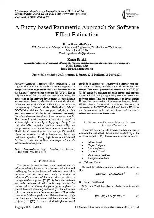
I.J. Modern Education and Computer Science, 2018, 3, 47-54Published Online March 2018 in MECS (/)DOI: 10.5815/ijmecs.2018.03.06A Fuzzy based Parametric Approach for SoftwareEffort EstimationH. Parthasarathi PatraSRF, Department of Computer Science and Engineering, Birla Institute of Technology,Mesra, Ranchi, IndiaEmail: hparthasarathi@Kumar RajnishAssociate Professor, Department of Computer Science and Engineering, Birla Institute of Technology,Mesra, Ranchi, IndiaEmail: krajnish@bitmesra.ac.inReceived: 13 November 2017; Accepted: 15 January 2018; Published: 08 March 2018Abstract—Accurate Software effort estimation is an ongoing challenge for the modern software engineers in computer science engineering since last 30 years due to the dynamic behavior of the software [1] [2][14]. This is only because of the time and cost estimation during the early stage of the software development is quite difficult and erroneous. So many algorithmic and non algorithmic techniques are used such as SLIM (Software life cycle management), Halstead Model, Bailey-Basil Model, COCOMO model and Function point analysis, etc, but does not estimate all kinds of software accurately. Nowadays these traditional techniques are not acceptable. This research work proposes a new fuzzy model to achieve higher accuracy by multiplying a fuzzy factor with the effort equation predicted empirically. As comparison to both model based and equation based, Model based estimation focused on specific models where as equation based techniques are based on traditional equations. Fuzzy logic is more suitable and flexible to meet the realistic challenges of today’s software estimation process.Index Terms—Fuzzy logic, Membership function, KLOC, MRE, MMRE, PREDI.I NTRODUCTIONThis paper focused to satisfy the need of today’s software industry by estimating the cost and effort and challenging the various issues and variations occurred in software size. Accuracy and timely estimation of software efforts is one of the most critical activities to manage a software project [7] [8]. As both over estimate and under estimate of software is very harmful for modern software industry this paper gives emphasis to predict the effort accurately and reliably. If the estimation is low then the software development team will be under pressure to finish the product and if the estimation is high then the most of the resources will be commuted to the projects [9][11][21]. It is very critical to implement novel methods to improve the accuracy of a software projects. So nowadays many models are used to estimate the efforts. This model proposed an extensive COCOMO [4] [5] [6] model by changing the scale factors and constant values a, b and multiplying a fuzzy factor to measure the software effort. This paper structured as follows: Section II describes the overview of existing techniques, Section III describes a frame work to estimate the efforts as comparing with COCOMO model, and Section IV relates the development tools and techniques and section V relates conclusion and future work.II.O VERVIEW OF D IFFERENT M ODELS U SED FORS OFTWARE E STIMATIONSince 1990 more than 20 different models are used to estimate the cost, effort, Duration and productivity of the software project [4] [5]. These are categorized as follows.∙Model based∙Expert Judgment∙Learning based∙Dynamic Based∙Regression Analysis∙Composite methodsA.Halstead ModelsHalstead formulate a relation to estimate the effort as [3].1.5()0.7()Effort E KLOC=⨯ (1) B.Bailey-Basil ModelBailey and Basil formulate a relation to estimate the efforts [2].1.16() 5.5()Effort E KLOC=⨯ (2)C.Walston -Felix ModelWalston and Felix developed a model to estimate the efforts taking 60 IBM projects and analyzing relationship between derived lines of codes, constitutes participation, customer oriented changes and new lines of code0.91() 5.2()Effort E KLOC=⨯ (3)0.36() 4.1()Duration D KLOC=⨯ (4)D.Doty Model (Kloc>9)1.047() 5.288()Effort E KLOC=⨯ (5) E.Sel ModelThe software engineering laboratory (SEL) of the University of Maryland has established a model to estimate the effort as0.93() 1.4()Effort E KLOC=⨯ (6)0.26() 4.6()Duration D KLOC=⨯ (7) F.Cocomo Ii ModelThis model formulate like1.1() 2.9()Effort E KLOC=⨯ (8)III.P ROPOSED M ODEL AND M ETHODOLOGYTill now none of the existing models can measure software efforts accurately in the modern software industry for all kind of software’s. In this paper we analyze a new empirical model for effort estimation. The cost drivers which are very from project to project, so we have taken different scale factor values and categories the cost drivers into project, product, personal and computer. Finally by multiplying a fuzzy factor value the efforts are calculated.A.Data CollectionFor this paper the data’s are collected from 60 NASA projects from different containers, 93 NASA projects from common NASA2 and 63 NASA projects from promise repository. These data sets are real project data sets and may be used for practical proposes and can be viewed from “The Promise Repository of Empirical Software Engineering Data”. /repo. North Carolina State University, Department of Computer Science B.Description About Proposed ModelThis model is based on empirical analysis of 216 NASA Projects of different repository and it includes the scale factors like personnel, complexity, environment, risks and constraints. It predicts effort, cost estimates and reliability using the statistical approaches like y =a ×(KLOC)b+ d to evaluate the cost, effort and duration empirically analyzing 216 real projects data of NASA. In this model we use a regression formula, with the parameters ‘a’ and ‘b’ which are derived from project dataset using deterministic and heuristic methods and optimizing the global solution. In this by the regression analysis we express the relationship between two variables and to estimate the dependent variable (i.e. Effort) based on independent variable (i.e. LOC) using simulated annealing algorithm [18].Simulated annealing algorithm might have been used to solve a wide range of optimization problems in artificial intelligence and other areas. But in this study we have used it as a simple way to implement the algorithm to derive the parameters a, b considering randomly chosen values. However, it would be inappropriate to solve a complex problem to illustrate how to use simulated annealing [17]. Thus, we have taken a two variable function of Equation 9 and have been used for instructive purposes. There may have other optimization methods, which are more appropriate to solve this second order equation, but this section is only trying to set the basics for proper use of simulated annealing [10][18][19].22(,)54F x y x y xy=++- (9)To get a better sense of the behavior of Equation 9, Fig.1 shows the simulation graph of this equation. Let suppose that the goal is to find the values of x and y that minimize f(x, y). Clearly the solution is any point (x, y) that lies on the circle that intersects f(x, y) with the plane z = 0.We normally use simulated annealing when the solution has many variables, and finding or visualizing the solutions in these cases is much more difficult than interpreting the 3-D plot of Fig.1 [18][19][20]Fig.1. (Simulation Graph)C. Proposed Algorithm DescriptionI. StartII. Read the project KLOC and actual effort as EIII. Follow the equation ()b E n a KLOC =⨯⨯ where a, b are constants and n is the no. of projects.IV. log()log ()KLOC E n A B log KLOC +=⨯+∑∑∑ V. 2log()log()log()((log()))KLOC E A KLOC B KLOC ⨯=⨯+⨯∑∑∑∑Where A=log (a) and B = b+1.VI. Use the steps 4 and 5 to estimate the parameter Value of a and b by the method of statistical Techniques using the data of real projects empirically VII. End.D. Evolution Of Proposed AlgorithmHere the authors make a convenient way to estimate the effort and the new cost driver values are taken empirically as shown in Table 2 The proposed approach provides more accurate estimation with the comparison of COCOMO model. Researchers may redefine the value of cost drivers further for better result. Individually analyzing organic, semi detached and embedded projects empirically we got the parameter value a, b as shown in Table 1Table 1. Predicted parameters for proposed modelThe formula used to calculate the effort is151()()b i Effort E a KLOC NEAF FF ==⨯⨯⨯∏ (10)Where NEAF is the new effort adjustment factors, which are new cost driver calculated by the author in this paper empirically as shown in Table 2 and FF is the fuzzy factor will be calculated using Fuzzy Inference System as shown in Table 4. E. Fuzzy LogicFuzzy Logic is based on four basic concepts Fuzzy sets, Linguistic Variables, Possibility distribution and fuzzy If-then rules. Fuzzy Sets are the sets with smooth b oundaries like “Partha is Smart” [0, 1]. Linguistic variables – consider the sentence “Customer service is poor” uses a fuzzy set “poor” to describe the quality. Here Customer service is the linguistic variable. Possibility distribution means the constraints on the value of a linguistic variable imposed by assigning it a fuzzy set i.e. KLOC (Ranges) = [0, 300]. Fuzzy if-then rules are the conditional statement to describe a functional mapping that generalizes a bidirectional control structure in two-valued logic [22]. F. Fuzzy Inference ProcessFuzzification[12]: A membership function (MF) is a curve that defines how each point in the input space (universe of discourse) is mapped to a membership value (or degree of membership) between 0 and 1.Logical Operators and if-then Rules : Fuzzy if-then rule statements are used to formulate the conditional statements for a specific output. For example a single fuzzy if-then rule assumes the form if x is M then y is N, Where M and N is linguistic values.Defuzzification: There are two types of fuzzy inference systems in the fuzzy logic toolbox: Mamdani-type and Sugeno-type. In this model we have used Mamdani Type Inference systemIV. D EVELOPMENT T OOLS A ND T ECHNIQUE In this paper we have used MATLAB 7.5 which is a high-performance language for technical computing. It integrates computation, visualization, and programming in an easy-to-use environment where problems and solutions are expressed in familiar mathematical notation. We have used the following properties of MATLAB in this paper.Math and computation Algorithm development Data acquisitionModeling and simulation.Data analysis, exploration, and visualizationScientific and engineering graphics using FuzzyLogicApplication development, including graphical userinterface building.Fuzzy Interface System (Mamdani) in fuzzy logicTool Box A. ImplementationThis research will implement the algorithm proposed by the author using the new effort drivers given in Table 2 using Mamdani Fuzzy Inference System (FIS) and the predicted effort will be compared with Constructive Cost Model (COCOMO). Fuzzy Triangular membership (trimf) function has been taken for implementation. The results were analyzed using the criterion MRE, MMRE (Mean Magnitude of Relative Error), RMSE and PRED. B. Research Methodology UsedIn this method we have selected a particular type of Fuzzy Inference System (Mamdani) as shown in Fig. 2 and define the input variables (KLOC and Mode) and output variable (Fuzzy Factor). Then we set the type of the membership functions for input variables and the type of the membership function for output variable as shown in Fig. 3, Fig. 4 and Fig. 5. Here we have used 37 rules in Rule Editor as shown in Fig.8 and the data is now translated into a set of if –then rules written in Rule editor. The detailed model structure is shown in the Fig. 6. The detail fuzzy frame work used is shown in Fig. 2.Table 2. New Effort Adjustment FactorSl N o Cost Driver Very Low LowNominalHigh Very High Extra High 1 Required Reliability 0.75 0.97 1 1.15 1.18 2 2 DB Size 0.86 0.96 1 1.01 1.18 1.9 3 Product complexity 0.7 0.99 1 1.19 1.2 1.23 4 Time constraint 0.78 0.85 1 1.35 1.38 1.86 5 Main Memory constraint 0.7 0.85 1 1.01 1.22 1.76 6 Machine volatility 0.8 0.93 1 1.01 1.3 1.55 7 Turnaroun d Time 0.8 0.93 1 1.09 1.34 - 8 Analyst Capability 1.46 1.19 1 0.86 0.78 - 9 Applicatio nexperience 1.29 1.23 1 0.95 0.94 - 10 Programm ercapability 1.42 1.17 1 0.96 0.95 - 11 Virtual Machine 1.34 1.01 1 0.82 - - 12 Language experience 1.02 0.98 1 0.92 - - 13 Modern programmi ng practice 1.24 1.14 1 0.94 0.81 - 14 Use of software tools 1.19 1.14 1 0.93 0.82 - 15Schedule constraint1.231.0311.081.1-Fig.2. Frame work for Fuzzy Interface SystemFig.3. MF for input variable KLOCFig.4. MF for input variable ModeFig.5. MF for output variable Fuzzy FactorFig.6. Fuzzy Inference SystemC. Performance Of The Proposed ModelTable 5 shows the result of effort estimation by the proposed model as comparison to COCOMO model and Table 3 shows the effort variance of different model in accordance with the data of 15 given projects andmeasure the performance to validate the outcome. Table 4 shows the performance of the proposed model using MMRE, RMSE and PRED with comparison to COCOMO models.Table 3. Effort Variance of different ModelsFig.7. Performance Graph (COCOMO Vs Proposed Model Table 4 Performance of COCOMO VS Proposed Model Fig.8. Rule Editor of Fuzzy Interface System Fig.9. Rule viewer of FISFig.10. Surface viewer of Fuzzy FactorD. Evaluation Criteria And Error Analysis [16]. There are so many statistical approaches are used to estimate the accuracy of the software effort. We are using methods like MRE, MMRE, RMSE, and Prediction. Boehm [2] suggested a formula to find out the error percentage as shown belowPr __%_edicted Effort Actual EffortError Actual Effort-=(11)MRE (Magnitude of relative error): We can calculate the degree of estimation error for individual project.|Pr __|_edicte Effort Actual Effort MRE Actual Effort-=(12)RMSE (Root Mean Square Error): we can calculate it as the square root of the mean square error and can be defined as.RMSEMMRE (Mean Magnitude of Relative Error): It is another way to measure the performance and it calculates the percentage of absolute values of relative errors. It is defined as.1|Pr __|1_edicted effort Actual Effort n MMRE i n Actual Effort -=∑= (14)PRED (N): This criteria is used to calculate the average percentage of estimates that were within N% of the actual values i.e. the percentage of predictions that fall within p % of the actual, denoted as PRED (p).Where k is the number of projects in which MRE is less than or equal to p, and n is the total number of projects. It is defined as PRED (p) = k / nFor project1 having KLOC =25.9 the actual effort is 117.6 Man-Month and the calculated effort for Basic COCOMO and Intermediate COCOMO is 100.86 MM and by the proposed model is 122.2 MM. Similarly for project 2 KLOC=24.6 the actual effort is 117.6 MM and calculated effort for Basic COCOMO and Intermediate COCOMO is 95.21 MM and by the proposed model is 115.3 MM. Now we can calculate the % of error using the equation 11. For project 1, the error % for Basic COCOMO and Intermediate COCOMO is (-14.23) % and error % for proposed model is (+3.91) %. Similarly For project 2, the error % for Basic COCOMO and Intermediate COCOMO is (-19.03) % and error % for proposed model is (-1.95) %. Here the negative %indicates the under estimation of the project and positive % error indicates the project is over estimate. Big under estimate gives extra pressure to the developing staff and leads to add more staffs which causes the late to fi nish the project. According to Parkinson’s Law “Work expands to fill the time available for its completion” Big over estimation reduces the productivity of personnel’s [15]. So during estimation the researchers should have to give emphasis to reduce the big over or under estimation of the project.E. Comparison With Cocomo Models[13]In software estimation COCOMO model is a regular and standard model to estimate the effort developed by Barry Boehm. But in the proposed model the researcher used a basic regression formula, with parameters that are derived from historical project (NASA software). Here we are estimating the effort based on the actual project characteristic data and better result predicts as compare to MMRE and RMSE as shown in Table 4. F. Advantages Of Proposed ModelIt Is reusableIt calculates software development effort as afunction of program size expressed in Kilo Lines of code (KLOC)It predicts the estimated effort with more accuracy.V. C ONCLUSION A ND F UTURE W ORKThis proposed model can be useful to estimate the software effort with better accuracy which is very important when software pays a lot in every industry. In this paper the author analyze more than 250 projects collected from PROMISE repository. The predicted result shows there is very close values between actual and estimated effort. The effort variance is very less and the proposed model has the lowest MMRE and RMSE and prediction values i.e. 0.03512 and 3.11 and 1.0 respectively. So the proposed model may able to provide good estim ation capabilities for today’s software ind ustry. A fuzzy model is more adaptive when the systems are not suitable for analysis by conventional approach or when the available data is uncertain, inaccurate or vague. The major difference between our work and previous works is that two fuzzy logic functions will be used for software development effort estimation on the model and then it’s validated with gathered data. The advantages of fuzzy logic are combined and learning ability and good generalization are obtained. The main benefit of this approach is it has good interpretability by using the fuzzy rules. The effort predicted using four fuzzy logic functions will be compared with Intermediate COCOMO.Table 5. Effort estimation by different ModelsR EFERENCES[1] Zia, Z.; Rashid, A “Software Cost Estimation forcomponent based fourth-generation- Language software applications”, IET software , vol.5 (2011), pp. 103-110 [2] Boehm, B. W. and Papaccio, P. N “Understanding andcontrolling software costs,” IEEE Transactions on Software Engineering, vol. 14(1988), no. 10.[3] Benediktsson, O. and Dalcher, D. “Effort Estimation inincremental Software Development,” IEEE Proc. Software, Vol. 150, no. 6(2003), pp. 351-357.[4] Boehm, B.W. “Software engineering economics ” (1981),Prentice –hall.[5] Srivastava, D.K.; Chauhan, D.S. and Singh,” R,SquareModel- A Software Process Model for IVR Software System ”- International Journal of Computer Application (0975-8887) Volume 13- No 7.(2011), 33- 36.[6] Jørgensen, M. and Sjøberg, D.I.K. “The impact ofcustomer expectation on software development effort estimates,” International Journal of Project Management , 22(4) (2004): pp. 317-325.[7] Set h, K and Sharma, A. “Effort Estimation Techniques inComponent based Development”- A Critical Review Proceedings of the 3rd National Conference , (2009) INDIACom.[8] Shepperd, M. and Schofield, C. “Estimating SoftwareProject Effort Using Analogies,” IEEE Transactions on Software Engineering , vol. 23, no. 12(1987), pp. 736-743.. [9] Maxwell, K.D. and Forselius, P.”Benchmarking SoftwareDevelopment Productivity ” IEEE Software , 17 (2000): pp. 80- 88.[10] Uysal, M. “Estimation of the Effort Component of theSoftware Projects Using Simulated Annealing Algorithm,” World Academy of Science, Engineering and Technology . (2008) [11] Moløkken-Østvold, K. and Jørgensen, M. “A Review ofSurveys on Software Effort Estimation.” ACM-IEEE International Symposium on Empirical Software Engineering. Frascati, Monte Porzio Catone (RM), ITALY: IEEE. (2003) pp. 220- 230[12] Attarzadeh,“A Novel Soft Computing Model to Increasethe Accuracy of Software Development Cost Estimation,” The 2nd International Conference on Computer and Automation Engineering ICCAE , (2010) p. 603-607[13] Singh, Y. and Aggarwal, K.K. “Software Engineering”Third edition, New Age International Publisher Limited New Delhi.(2005)[14] Deshpande, M.V. and Bhirud, S.G. “Analysis ofCombining Software Estimation Techniques,” International journal of Computer Applications (0975 – 8887) Volume 5 – No.3.[15] Jolte, P. “An Integrated Approach to SoftwareEngineering .” Third edition Narosa Publishing house New Delhi.[16] Pressman. “Software Engineering - a Practitioner’sApproach ”. 6th Edition McGraw Hill international Edition, Pearson education, ISBN 007 -124083. [17] Suri, P.K.; Bharat, B. Time Estimation for ProjectManagement Life Cycle: A Simulation approach, International Journal of Computer Science and Network Security , VOL.9 No.5. (2009)”[18] Se rgio, L.; Gabriel, A. and Raul, S.”Practicalconsideration of simulated annealing Implementation”, Cher Ming Tan (Ed.), ISBN: 978-953-7619-07-7 (2008). [19] Montaz, A.; Aimo, T. and Sami, V”A Direct searchsimulated annealing algorithm for optimization involving continuous variables ”Turku center of computer science, Technical Report No-97(1997).[20] Tushar, G. and Nielen, S.”Adaptive simulated annealingfor global optimization”, Livermore software technology corporation, USA, 7th European LS-DYNA conference ,(2009).[21] Ziauddin, Shahid K., Shafiullah K. and Jamal A. N. (2013)“A Fuzzy Logic Based Software Cost Estimation Model “International Journal of Software Engineering and Its Applications Vol. 7, No. 2.[22] Babuska, R. “Fuzzy Modeling and Identification ToolboxUser’s Guide” (August 1998).Authors ’ ProfilesH Parthasarathi Patra, He is a Research scholar, Department of computer Science, Birla Institute of Technology, Mesra, Ranchi. Jharkhand, India. He received his ME (Software Engineering) Degree from Jadavpur University, West Bengal, India in the year 2011. He received his B.Tech (IT) from BPUT, Odisha, India in the year 2005. He has 10 International ResearchPublications. His Research area is Software Engineering, Software Quality Metrics, measurement and Estimation, Programming Languages, and Database Study.Dr. Kumar Rajnish, He is an Associate professor in the Department of Computer Science and Engineering at Birla Institute of Technology, Mesra. He received his B.Sc Maths (Honours) in the year 1998 from Ranchi College Ranchi (Ranchi University) state of Jharkhand, India, Master of Computer Application (MCA) in the year 2001 in Department ofComputer Science and Engineering from Madan Mohan Malaviya Engineering College, Gorakhpur (Deen Dayal Gorakpur University) Uttar Pradesh (U.P) India. He has 40 International and National Research Publications. His research interests are Object-Oriented Metrics, Object-Oriented Software Engineering, Programming languages, Database, and Operating System.How to cite this paper: H. Parthasarathi Patra, Kumar Rajnish, " A Fuzzy based Parametric Approach for Software Effort Estimation", International Journal of Modern Education and Computer Science(IJMECS), Vol.10, No.3, pp. 47-54, 2018.DOI: 10.5815/ijmecs.2018.03.06。

E1 –European digital transmission channel with a data rate of 2.048 kbps. EACEM –European Association of Consumer Electronics Manufacturers EAPROM (Electrically Alterable Programmable Read-Only Memo) –A PROM whose contents can be changed.E arth Station –Equipment used for transmitting or receiving satellite communications.EAV (End of Active Video) –A term used with component digital systems.EB (Errored Block)EBR –See Electron Beam Recording.EBU (European Broadcasting Union) –An organization of European broadcasters that,among other activities,produces technical statements and recommendations for the 625/50 line televi-sion system.Created in 1950 and headquartered in Geneva,Switzerland,the EBU is the world’s largest professional association of national broadcasters.The EBU assists its members in all areas of broadcasting,briefing them on developments in the audio-visual sector,providing advice and defending their interests via international bodies.The Union has active members in European and Mediterranean countries and associate members in countries elsewherein Africa,the Americas and Asia.EBU TECH.3267-E – a)The EBU recommendation for the serial composite and component interface of 625/50 digital video signal including embed-ded digital audio.b)The EBU recommendation for the parallel interface of 625 line digital video signal.A revision of the earlier EBU Tech.3246-E, which in turn was derived from CCIR-601 and contributed to CCIR-656 standards.EBU Timecode –The timecode system created by the EBU and based on SECAM or PAL video signals.ECC (Error Correction Code) –A type of memory that corrects errors on the fly.ECC Constraint Length –The number of sectors that are interleaved to combat bursty error characteristics of discs.16 sectors are interleaved in DVD.Interleaving takes advantage of typical disc defects such as scratch marks by spreading the error over a larger data area,thereby increasing the chance that the error correction codes can conceal the error.ECC/EDC (Error Correction Code/Error Detection Code) –Allows data that is being read or transmitted to be checked for errors and,when nec-essary,corrected on the fly.It differs from parity-checking in that errors are not only detected but also corrected.ECC is increasingly being designed into data storage and transmission hardware as data rates (and therefore error rates) increase.Eccentricity –A mathematical constant that for an ellipse is the ratio between the major and minor axis length.more points in the transmission medium,with sufficient magnitude and time difference to be perceived in some manner as a wave distinct from that of the main or primary transmission.Echoes may be either leading or lagging the primary wave and appear in the picture monitor as reflections or “ghosts”.b)Action of sending a character input from a keyboard to the printer or display.Echo Cancellation –Reduction of an echo in an audio system by estimating the incoming echo signal over a communications connection and subtracting its effects from the outgoing signal.Echo Plate –A metal plate used to create reverberation by inducing waves in it by bending the metal.E-Cinema –An HDTV film-complement format introduced by Sony in 1998.1920 x 1080,progressive scan,24 fps,4:4:4 ing a 1/2-inch tape,the small cassette (camcorder) will hold 50 minutes while the large cassette will hold 156 minutes.E-Cinema’s camcorder will use three 2/3-inch FIT CCDs and is equivalent to a film sensitivity of ISO 500. The format will compress the electronic signal somewhere in the range of 7:1.The format is based on the Sony HDCAM video format.ECL (Emitter Coupled Logic) –A variety of bipolar transistor that is noted for its extremely fast switching speeds.ECM –See Entitlement Control Message.ECMA (European Computer Manufacturers Association) –An international association founded in 1961 that is dedicated to establishing standards in the information and communications fields.ECMA-262 –An ECMA standard that specifies the core JavaScript language,which is expected to be adopted shortly by the International Standards Organization (ISO) as ISO 16262.ECMA-262 is roughly equivalent to JavaScript 1.1.ECU (Extreme Closeup)ED-Beta (Extended Definition Betamax) –A consumer/Professional videocassette format developed by Sony offering 500-line horizontal resolution and Y/C connections.Edge – a)An edge is the straight line that connects two points.b)Synonym for key ed by our competitors but not preferred by Ampex.c)A boundary in an image.The apparent sharpness of edges can be increased without increasing resolution.See also Sharpness.Edge Busyness –Distortion concentrated at the edge of objects, characterized by temporally varying sharpness or spatially varying noise.Edge Curl –Usually occurs on the outside one-sixteenth inch of the videotape.If the tape is sufficiently deformed it will not make proper tape contact with the playback heads.An upper curl (audio edge) crease may affect sound quality.A lower edge curl (control track) may result in poor picture quality.Edge Damage –Physical distortion of the top or bottom edge of the mag-netic tape,usually caused by pack problems such as popped strands or stepping.Affects audio and control track sometimes preventing playback. Edge Effect –See Following Whites or Following Blacks.Edge Enhancement –Creating hard,crisp,high-contrast edges beyond the correction of the geometric problem compensated by aperture correc-tion,frequently creates the subjective impression of increase image detail. Transversal delay lines and second-directive types of correction increase the gain at higher frequencies while introducing rather symmetrical “under-shoot followed by overshoot”at transitions.In fact,and contrary to many causal observations,image resolution is thereby decreased and fine detail becomes obscured.Creating a balance between the advantages and disad-vantages is a subjective evaluation and demands an artistic decision. Edge Enhancing –See Enhancing.Edge Filter –A filter that applies anti-aliasing to graphics created to the title tool.Edge Numbers – Numbers printed on the edge of 16 and 35 mm motion picture film every foot which allows frames to be easily identified in an edit list.Edgecode –See Edge Numbers,Key Numbers.EDH (Error Detection and Handling) –Defined by SMPTE standards RP-165 and is used for recognizing inaccuracies in the serial digital signal. It may be incorporated into serial digital equipment and employ a simple LED error indicator.This data conforms to the ancillary data formatting standard (SMPTE 291M) for SD-SDI and is located on line 9 for 525 and line 5 for 625 formats.Edit – a) The act of performing a function such as a cut,dissolve,wipe on a switcher,or a cut from VTR to VTR where the end result is recorded on another VTR.The result is an edited recording called a master.b)Any point on a video tape where the audio or video information has been added to, replaced,or otherwise altered from its original form.Edit Control –A connection on a VCR or camcorder which allows direct communication with external edit control devices.(e.g.,LANC (Control-L) and new (Panasonic) 5-pin).Thumbs Up works with both of these control formats and with machines lacking direct control.Edit Controller –An electronic device,often computer-based,that allows an editor to precisely control,play and record to various videotape machines.Edit Decision List (EDL) – a)A list of a video production’s edit points. An EDL is a record of all original videotape scene location time references, corresponding to a production’s transition events.EDLs are usually generated by computerized editing equipment and saved for later use and modification.b) Record of all edit decisions made for a video program (such as in-times,out-times,and effects) in the form of printed copy, paper tape,or floppy disk file,which is used to automatically assemble the program at a later point.Edit Display –Display used exclusively to present editing data and editor’s decision lists.Edit Master –The first generation (original) of a final edited tape.Edit Point –The location in a video where a production event occurs. (e.g.,dissolve or wipe from one scene to another).Edit Rate –In compositions,a measure of the number of editable units per second in a piece of media data (for example,30 fps for NTSC,25 fps for PAL and 24 fps for film).Edit Sequence –An assembly of clips.Editing –A process by which one or more compressed bit streams are manipulated to produce a new compressed bit stream.Conforming edited bit streams are understood to meet the requirements defined in the Digital Television Standard.Editing Control Unit (ECU) –A microprocessor that controls two or more video decks or VCRs and facilitates frame-accurate editing.Editor –A control system (usually computerized) which allows you to con-trol video tape machines,the video switcher,and other devices remotely from a single control panel.Editors enable you to produce finished video programs which combine video tape or effects from several different sources.EDL (Edit Decision List) –A list of edit decisions made during an edit session and usually saved to floppy disk.Allows an edit to be redone or modified at a later time without having to start all over again.EDO DRAM (Extended Data Out Dynamic Random Access Memory) –EDO DRAM allows read data to be held past the rising edge of CAS (Column Address Strobe) improving the fast page mode cycle time critical to graphics performance and bandwidth.EDO DRAM is less expensive than VRAM.EDTV –See Extended/Enhanced Definition Television.E-E Mode (Electronic to Electronic Mode) –The mode obtained when the VTR is set to record but the tape is not running.The VTR is processing all the signals that it would normally use during recording and playback but without actually recording on the tape.EEprom E2,E’squared Prom –An electronically-erasable,programmable read-only memory device.Data can be stored in memory and will remain there even after power is removed from the device.The memory can be erased electronically so that new data can be stored.Effect – a)One or more manipulations of the video image to produce a desired result.b)Multi-source transition,such as a wipe,dissolve or key. Effective Competition –Market status under which cable TV systems are exempt from regulation of basic tier rates by local franchising authorities, as defined in 1992 Cable Act.To claim effective competition,a cable system must compete with at least one other multi-channel provider that is available to at least 50% of an area’s households and is subscribed to by more than 15% of the households.Effects –The manipulation of an audio or video signal.Types of film or video effects include special effects (F/X) such as morphing; simple effects such as dissolves,fades,superimpositions,and wipes; complex effects such as keys and DVEs; motion effects such as freeze frame and slow motion; and title and character generation.Effects usually have to be rendered because most systems cannot accommodate multiple video streams in real time.See also Rendering.Effects (Setup) –Setup on the AVC,Century or Vista includes the status of every push-button,key setting,and transition rate.The PANEL-MEM system can store these setups in memory registers for future use.Effects Keyer (E Keyer) –The downstream keyer within an M/E,i.e.,the last layer of video.Effects System –The portion of the switcher that performs mixes,wipes and cuts between background and/or affects key video signals.The Effects System excludes the Downstream Keyer and Fade-to-Black circuitry.Also referred to as Mix Effects (M/E) system.EFM (Eight-to-Fourteen Modulation) –This low-level and very critical channel coding technique maximizes pit sizes on the disc by reducing frequent transitions from 0 to 1 or 1 to 0.CD represents 1's as Land-pit transitions along the track.The 8/14 code maps 8 user data bits into 14 channel bits in order to avoid single 1's and 0's,which would otherwise require replication to reproduce extremely small artifacts on the disc.In the 1982 compact disc standard (IEC 908 standard),3 merge bits are added to the 14 bit block to further eliminate 1-0 or 0-1 transitions between adjacent 8/14 blocks.EFM Plus –DVD’s EFM+ method is a derivative of EFM.It folds the merge bits into the main 8/16 table.EFM+ may be covered by U.S.Patent5,206,646.EGA (Enhanced Graphics Adapter) –A display technology for the IBM PC.It has been replaced by VGA.EGA pixel resolution is 640 x 350.EIA (Electronics Industries Association) –A trade organization that has created recommended standards for television systems (and other electronic products),including industrial television systems with up to 1225 scanning lines.EIA RS-170A is the current standard for NTSC studio equipment.The EIA is a charter member of ATSC.EIA RS-170A –The timing specification standard for NTSC broadcast video equipment.The Digital Video Mixer meets RS-170A.EIA/IS-702 –NTSC Copy Generation Management System – Analog (CGMS-A).This standard added copy protection capabilities to NTSC video by extending the EIA-608 standard to control the Macrovision anti-copy process.It is now included in the latest EIA-608 standard.EIA-516 –U.S.teletext standard,also called NABTS.EIA-608 –U.S.closed captioning and extended data services (XDS) stan-dard.Revision B adds Copy Generation Management System – Analog (CGMS-A),content advisory (v-chip),Internet Uniform Resource Locators (URLs) using Text-2 (T-2) service,16-bit Transmission Signal Identifier,and transmission of DTV PSIP data.EIA-708 –U.S.DTV closed captioning standard.EIA CEB-8 also provides guidance on the use and processing of EIA-608 data streams embedded within the ATSC MPEG-2 video elementary transport stream,and augments EIA-708.EIA-744 –NTSC “v-chip”operation.This standard added content advisory filtering capabilities to NTSC video by extending the EIA-608 standard.It is now included in the latest EIA-608 standard,and has been withdrawn. EIA-761 –Specifies how to convert QAM to 8-VSB,with support for OSD (on screen displays).EIA-762 –Specifies how to convert QAM to 8-VSB,with no support for OSD (on screen displays).EIA-766 –U.S.HDTV content advisory standard.EIA-770 –This specification consists of three parts (EIA-770.1,EIA-770.2, and EIA-770.3).EIA-770.1 and EIA-770.2 define the analog YPbPr video interface for 525-line interlaced and progressive SDTV systems.EIA-770.3 defines the analog YPbPr video interface for interlaced and progressive HDTV systems.EIA-805 defines how to transfer VBI data over these YPbPr video interfaces.EIA-775 –EIA-775 defines a specification for a baseband digital interface to a DTV using IEEE 1394 and provides a level of functionality that is simi-lar to the analog system.It is designed to enable interoperability between a DTV and various types of consumer digital audio/video sources,including set top boxes and DVRs or VCRs.EIA-775.1 adds mechanisms to allow a source of MPEG service to utilize the MPEG decoding and display capabili-ties in a DTV.EIA-775.2 adds information on how a digital storage device, such as a D-VHS or hard disk digital recorder,may be used by the DTVor by another source device such as a cable set-top box to record or time-shift digital television signals.This standard supports the use of such storage devices by defining Service Selection Information (SSI),methods for managing discontinuities that occur during recording and playback, and rules for management of partial transport streams.EIA-849 specifies profiles for various applications of the EIA-775 standard,including digital streams compliant with ATSC terrestrial broadcast,direct-broadcast satellite (DBS),OpenCable™,and standard definition Digital Video (DV) camcorders.EIA-805 –This standard specifies how VBI data are carried on component video interfaces,as described in EIA-770.1 (for 480p signals only),EIA-770.2 (for 480p signals only) and EIA-770.3.This standard does not apply to signals which originate in 480i,as defined in EIA-770.1 and EIA-770.2. The first VBI service defined is Copy Generation Management System (CGMS) information,including signal format and data structure when car-ried by the VBI of standard definition progressive and high definition YPbPr type component video signals.It is also intended to be usable when the YPbPr signal is converted into other component video interfaces including RGB and VGA.EIA-861 – The EIA-861 standard specifies how to include data,such as aspect ratio and format information,on DVI and HDMI.EIAJ (Electronic Industry Association of Japan) –The Japanese equivalent of the EIA.EIA-J CPR-1204 –This EIA-J recommendation specifies another widescreen signaling (WSS) standard for NTSC video signals.E-IDE (Enhanced Integrated Drive Electronics) –Extensions to the IDE standard providing faster data transfer and allowing access to larger drives,including CD-ROM and tape drives,using ATAPI.E-IDE was adopted as a standard by ANSI in 1994.ANSI calls it Advanced Technology Attachment-2 (ATA-2) or Fast ATA.EISA (Enhanced Industry Standard Architecture) –In 1988 a consor-tium of nine companies developed 32-bit EISA which was compatible with AT architecture.The basic design of EISA is the result of a compilation of the best designs of the whole computer industry rather than (in the case ofthe ISA bus) a single company.In addition to adding 16 new data linesto the AT bus,bus mastering,automated setup,interrupt sharing,and advanced transfer modes were adapted making EISA a powerful and useful expansion design.The 32-bit EISA can reach a peak transfer rate of33 MHz,over 50% faster than the Micro Channel architecture.The EISA consortium is presently developing EISA-2,a 132 MHz standard.EISA Slot –Connection slot to a type of computer expansion bus found in some computers.EISA is an extended version of the standard ISA slot design.EIT (Encoded Information Type)EIT (Event Information Table) –Contains data concerning events (a grouping of elementary broadcast data streams with a defined start and end time belonging to a common service) and programs (a concatenation of one or more events under the control of a broadcaster,such as event name,start time,duration,etc.).Part of DVB-SI.Electromagnetic Interference (EMI) –Interference caused by electrical fields.Electron Beam Recording –A technique for converting television images to film using direct stimulation of film emulsion by a very fine long focal length electronic beam.E lectronic Beam Recorder (EBR) –Exposes film directly using an electronic beam compared to recording from a CRT.Electronic Cinematography –Photographing motion pictures with television equipment.Electronic cinematography is often used as a term indicating that the ultimate product will be seen on a motion picture screen,rather than a television screen.See also HDEP and Mathias.Electronic Crossover –A crossover network which uses active filters and is used before rather than after the signal passes through the power amp.Electronic Editing –The assembly of a finished video program in which scenes are joined without physically splicing the tape.Electronic editing requires at least two decks:one for playback and the other for recording. Electronic Matting –The process of electronically creating a composite image by replacing portions of one image with another.One common,if rudimentary,form of this process is chroma-keying,where a particular color in the foreground scene (usually blue) is replaced by the background scene.Electronic matting is commonly used to create composite images where actors appear to be in places other than where they are being shot. It generally requires more chroma resolution than vision does,causing contribution schemes to be different than distribution schemes.While there is a great deal of debate about the value of ATV to viewers,there does not appear to be any dispute that HDEP can perform matting faster and better than almost any other moving image medium.Electronic Pin Register (EPR) –Stabilizes the film transport of a telecine.Reduces ride (vertical moment) and weave (horizontal movement). Operates in real time.Electrostatic Pickup –Pickup of noise generated by electrical sparks such as those caused by fluorescent lights and electrical motors. Elementary Stream (ES) – a)The raw output of a compressor carrying a single video or audio signal.b)A generic term for one of the coded video,coded audio,or other coded bit streams.One elementary stream is carried in a sequence of PES packets with one and only one stream_id.Elementary Stream Clock Reference (ESCR) –A time stamp in the PES from which decoders of PES may derive timing.Elementary Stream Descriptor –A structure contained in object descriptors that describes the encoding format,initialization information, transport channel identification,and other descriptive information about the content carried in an elementary stream.Elementary Stream Header (ES Header) –Information preceding the first data byte of an elementary stream.Contains configuration information for the access unit header and elementary stream properties.Elementary Stream Interface (ESI) –An interface modeling the exchange of elementary stream data and associated control information between the Compression Layer and the Sync Layer.Elementary Stream Layer (ES Layer) –A logical MPEG-4 Systems Layer that abstracts data exchanged between a producer and a consumer into Access units while hiding any other structure of this data.Elementary Stream User (ES User) –The MPEG-4 systems entity that creates or receives the data in an elementary stream.ELG (European Launching Group) –Now superseded by DVB.EM (Electronic Mail) –Commonly referred to as E-mail.Embedded Audio – a)Embedded digital audio is mul-tiplexed onto a seri-al digital data stream within the horizontal ancillary data region of an SDI signal.A maximum of 16 channels of audio can be carried as standardized with SMPTE 272M or ITU-R.BT.1305 for SD and SMPTE 299 for HD.b)Digital audio that is multiplexed and carried within an SDI connection –so simplifying cabling and routing.The standard (ANSI/SMPTE 272M-1994) allows up to four groups each of four mono audio channels.Embossing –An artistic effect created on AVAs and/or switchers to make characters look like they are (embossed) punched from the back of the background video.EMC (Electromagnetic Compatibility) –Refers to the use of compo-nents in electronic systems that do not electrically interfere with each other.See also EMI.EMF (Equipment Management Function) –Function connected toall the other functional blocks and providing for a local user or the Telecommunication Management Network (TMN) a mean to perform all the management functions of the cross-connect equipment.EMI (Electromagnetic Interference) –An electrical disturbance in a sys-tem due to natural phenomena,low-frequency waves from electromechani-cal devices or high-frequency waves (RFI) from chips and other electronic devices.Allowable limits are governed by the FCC.See also EMC. Emission – a)The propagation of a signal via electromagnetic radiation, frequently used as a synonym for broadcast.b) In CCIR usage:radio-frequency radiation in the case where the source is a radio transmitteror radio waves or signals produced by a radio transmitting station.c) Emission in electronic production is one mode of distribution for the completed program,as an electromagnetic signal propagated to thepoint of display.EMM –See Entitlement Management Message.E-Mode –An edit decision list (EDL) in which all effects (dissolves,wipes and graphic overlays) are performed at the end.See also A-Mode,B-Mode, C-Mode,D-Mode,Source Mode.Emphasis – a)Filtering of an audio signal before storage or transmission to improve the signal-to-noise ratio at high frequencies.b)A boost in signal level that varies with frequency,usually used to improve SNRin FM transmission and recording systems (wherein noise increaseswith frequency) by applying a pre-emphasis before transmission and a complementary de-emphasis to the receiver.See also Adaptive Emphasis. Emulate –To test the function of a DVD disc on a computer after format-ting a complete disc image.Enable –Input signal that allows the device function to occur.ENB (Equivalent Noise Bandwidth) –The bandwidth of an ideal rectan-gular filter that gives the same noise power as the actual system. Encode – a)The process of combining analog or digital video signals, e.g.,red,green and blue,into one composite signal.b)To express a single character or a message in terms of a code.To apply the rules of a code. c)To derive a composite luminance-chrominance signal from R,G,B signals.d)In the context of Indeo video,the process of converting the color space of a video clip from RGB to YUV and then compressing it.See Compress,RGB,pare Decode.Encoded Chroma Key –Synonym for Composite Chroma Key. Encoded Subcarrier –A reference system created by Grass Valley Group to provide exact color timing information.Encoder – a)A device used to form a single composite color signal (NTSC,PAL or SECAM) from a set of component signals.An encoder is used whenever a composite output is required from a source (or recording) which is in component format.b)Sometimes devices that change analog signals to digital (ADC).All NTSC cameras include an encoder.Because many of these cameras are inexpensive,their encoders omit many ofthe advanced techniques that can improve NTSC.CAV facilities canuse a single,advanced encoder prior to creating a final NTSC signal.c)An embodiment of an encoding process.Encoding (Process) –A process that reads a stream of input pictures or audio samples and produces a valid coded bit stream as defined in the Digital Television Standard.Encryption – a) The process of coding data so that a specific code or key is required to restore the original data.In broadcast,this is used to make transmission secure from unauthorized reception as is often found on satellite or cable systems.b) The rearrangement of the bit stream of a previously digitally encoded signal in a systematic fashion to make the information unrecognizable until restored on receipt of the necessary authorization key.This technique is used for securing information transmit-ted over a communication channel with the intent of excluding all other than authorized receivers from interpreting the message.Can be used for voice,video and other communications signals.END (Equivalent Noise Degradation)End Point –End of the transition in a dissolve or wipe.Energy Plot –The display of audio waveforms as a graph of the relative loudness of an audio signal.ENG (Electronic News Gathering) –Term used to describe use of video-recording instead of film in news coverage.ENG Camera (Electronic News Gathering camera) –Refers to CCD cameras in the broadcast industry.Enhancement Layer –A relative reference to a layer (above the base layer) in a scalable hierarchy.For all forms of scalability,its decoding process can be described by reference to the lower layer decoding process and the appropriate additional decoding process for the Enhancement Layer itself.Enhancing –Improving a video image by boosting the high frequency content lost during recording.There are several types of enhancement. The most common accentuates edges between light and dark images. ENRZ (Enhanced Non-Return to Zero)Entitlement Control Message (ECM) –Entitlement control messages are private conditional access information.They are program-specific and specify control and scrambling parameters.Entitlement Management Message (EMM) –Private Conditional Access information which specifies the authorization levels or the services of specific decoders.They may be addressed to individual decoder or groups of decoders.Entrophy –The average amount of information represented by a symbol in a message.It represents a lower bound for compression.Entrophy Coding –Variable-length lossless coding of the digital represen-tation of a signal to reduce redundancy.Entrophy Data –That data in the signal which is new and cannot be compressed.Entropy –In video,entropy,the average amount of information represent-ed by a symbol in a message,is a function of the model used to produce that message and can be reduced by increasing the complexity of the model so that it better reflects the actual distribution of source symbolsin the original message.Entropy is a measure of the information contained in a message,it’s the lower bound for compression.Entry –The point where an edit will start (this will normally be displayed on the editor screen in time code).Entry Point –The point in a coded bit stream after which the decoder can be initialized and begin decoding correctly.The picture that follows the entry point will be an I-picture or a P-picture.If the first transmitted picture is not an I-picture,the decoder may produce one or more pictures during acquisition.Also referred to as an Access Unit (AU).E-NTSC –A loosely applied term for receiver-compatible EDTV,used by CDL to describe its Prism 1 advanced encoder/decoder family.ENTSC –Philips ATV scheme now called HDNTSC.Envelope Delay –The term “Envelope Delay”is often used interchange-ably with Group Delay in television applications.Strictly speaking,envelope delay is measured by passing an amplitude modulated signal through the system and observing the modulation envelope.Group Delay on the other。

专业英语[单项选择题]1、 A project life cycle is a collection of generally sequential project（）(1) whose name and number are determined by the control needs of the organization or organizations involved in the project. The life cycle provides the basic （）(2) for managing the project, regardless of the specific work involved. 空白（2）处应选择（）A.planB.fractionC.mainD.framework参考答案：D[单项选择题]2、 A project life cycle is a collection of generally sequential project（）(1) whose name and number are determined by the control needs of the organization or organizations involved in the project. The life cycle provides the basic （）(2) for managing the project, regardless of the specific work involved. 空白（1）处应选择（）A.phasesB.processesC.segmentsD.pieces参考答案：A[单项选择题]3、 The（）process analyzes the effect of risk events and assigns a numerical rating to those risks.A.Risk IdentificationB.Quantitative Risk AnalysisC.Qualitative Risk AnalysisD.Risk Monitoring and Control参考答案：B[单项选择题]4、 Project（） Management is the Knowledge Area that employs theprocesses required to ensure timely and appropriate generation, collection, distribution, storage, retrieval, and ultimate disposition of project information.A.IntegrationB.TimeC.Planningmunication参考答案：B[单项选择题]5、（）is a category assigned to products or services having the same functional use but different technical characteristics. It is not same as quality.A.ProblemB.GradeC.RiskD.Defect参考答案：D[单项选择题]6、 Project Quality Management must address the management of the project and the（） of the project. While Project Quality Management applies to all projects, regardless of the nature of their product, product quality measures and techniques are specific to the particular type of product produced by the project.A.performanceB.processC.productD.object参考答案：B[单项选择题]7、 In approximating costs, the estimator considers the possible causes of variation of the cost estimates, including（） .A.budgetB.planC.riskD.contract参考答案：C[单项选择题]8、 On some projects, especially ones of smaller scope, activity sequencing, activity resource estimating, activity duration estimating, and （） are so tightly linked that they are viewed as a single process that can be performed by a person over a relatively short period of time.A.time estimatingB.cost estimatingC.project planningD.schedule development参考答案：C[单项选择题]9、 Project （） Management includes the processes required to ensure that the project includes all the work required, and only the work required, to complete the project successfully.A.IntegrationB.ScopeC.ConfigurationD.Requirement参考答案：D[单项选择题]10、 In the project management context,（） includes characteristics of unification, consolidation, articulation, and integrative actions that are crucial to project completion, successfully meeting customer and other stakeholder requirements, and managing expectations.A.IntegrationB.ScopeC.ConfigurationD.Requirement参考答案：B[单项选择题]11、 Organizations perform work to achieve a set of objectives. Generally, work can be categorized as either projects or operations, although the two sometimes are（）A.confusedB.sameC.overlapD.dissever[单项选择题]12、（）from one phase are usually reviewed for completeness and accuracy and approved before work starts on the next phase.A.ProcessestoneC.WorkD.Deliverables参考答案：C[单项选择题]13、（）involves comparing actual or planned project practices to those of other projects to generate ideas for improvement and to provide a basis by which to measure performance. These other projects can be within the performing organization or outside of it, and can be within the same or in another application area.A.MetricsB.MeasurementC.BenchmarkingD.Baseline参考答案：D[单项选择题]14、（）is the budgeted amount for the work actually completed on the schedule activity or WBS component during a given time period.A.Planned valueB.Earned valueC.Actual costD.Cost variance参考答案：C[单项选择题]15、 PDM includes four types of dependencies or precedence relationships: （）. The completion of the successor activity depends upon the initiation of the predecessor activity.A.Finish-to-StartB.Finish-to-FinishC.Start-to-StartD.Start-to-Finish[单项选择题]16、 The process of（）schedule activity durations uses information on schedule activity scope of work, required resource types, estimated resource quantities, and resource calendars with resource availabilities.A.estimatingB.definingC.planningD.sequencing参考答案：D[单项选择题]17、 The （） describes, in detail, the project's deliverables and the work required to create those deliverables.A.project scope statementB.project requirementC.project charterD.product specification参考答案：A[单项选择题]18、The（）provides the project manager with the authority to apply organizational resources to project activities.A.project management planB.contractC.project human resource planD.project charter参考答案：D参考解析：项目章程(project charter)为项目经理使用组织资源进行项目活动提供了授权。

Feasibility Report SampleIn the realm of business and project management, conducting feasibility studies is a crucial step in determining the viability of a proposed project or initiative. A feasibility report serves as a comprehensive assessment that evaluates various aspects of the project to determine if it is feasible and worth pursuing. This report outlines the key components of a typical feasibility study and provides insight into the process of assessing the feasibility of a project. IntroductionThe purpose of this feasibility report is to assess the viability of implementing a new marketing strategy for a multinational corporation looking to expand its market share in the Asia-Pacific region. The objective of the proposed project is to increase brand awareness, customer engagement, and ultimately drive sales in the target market.Market AnalysisA thorough market analysis is essential in determining the feasibility of the proposed marketing strategy. This includes an evaluation of the target market, competitive landscape, consumer behavior, and market trends. The Asia-Pacific region offers significant growth opportunities for the company, with a large and diverse consumer base. However, intense competition and cultural differences must be taken into consideration when developing the marketing strategy. Technical FeasibilityThe technical feasibility of the project involves assessing the resources, technology, and infrastructure required to implement the new marketing strategy. This includes evaluating the company's existing marketing capabilities, the availability of skilled personnel, and the need for any additional technology or tools to support the initiative. A thorough analysis of the technical aspects is crucial to ensure the successful implementation of the project.Financial AnalysisA comprehensive financial analysis is a critical component of the feasibility report. This involves estimating the costs associated with implementing the new marketing strategy, including advertising, promotional activities, personnel expenses, and technology investments. Additionally, revenue projections and return on investment (ROI) calculations are essential in determining the financial viability of the project. A detailed financial analysis helps in assessing the potential risks and rewards of the proposed initiative.Risk AssessmentIdentifying and evaluating potential risks is essential in assessing the feasibility of the project. Risks may arise from various sources, including market volatility, regulatory changes, competitive pressures, and internal challenges. Conducting a thorough risk assessment enables the project team to develop mitigation strategies and contingency plans to address potential challenges that may impact the success of the project.ConclusionIn conclusion, the feasibility report provides a comprehensive assessment of the proposed marketing strategy for the multinational corporation in the Asia-Pacific region. The analysis of market dynamics, technical requirements, financial implications, and risk factors suggests that the project is feasible and has the potential to yield positive results for the company. However, it is essential to address the identified risks and challenges effectively to ensure the successful implementation of the new marketing strategy.Overall, the feasibility report serves as a valuable tool for decision-makers to evaluate the potential of a project and make informed choices regarding its implementation. Conducting a thorough feasibility study helps in minimizing risks, maximizing opportunities, and ultimately achieving the desired outcomes.。

Income inequality and efficiency:A decomposition approach andapplications to ChinaYuk-shing Cheng *,Sung-ko LiDepartment of Economics,Hong Kong Baptist University,Renfrew Road,Kowloon Tong,Hong Kong,ChinaReceived 15October 2004;received in revised form 5July 2005;accepted 1September 2005AbstractThis paper suggests a new interpretation for a decomposition of the Theil inequality index when income can be expressed as multiplicative components.Applying the method to China,we find that the impact of technical inefficiency on inter-regional inequality has shown a declining trend.D 2005Elsevier B.V .All rights reserved.Keywords:Inequality;Decomposition;China;Technical efficiencyJEL classification:C10;D63;H731.IntroductionThis paper suggests a new interpretation for the residual term of a decomposition of the Theil index (or called Theil’s second measure)to identify the inequality contribution of multiplicative components of income.Our motivation is to find out the extent to which differentials in productivity and efficiency can explain China’s inter-provincial income inequality.We express income per capita in each region as the multiplication of productivity and efficiency terms.However,in the existing literature,decomposition of inequality when income is expressed as multiplicative components has not been 0165-1765/$-see front matter D 2005Elsevier B.V .All rights reserved.doi:10.1016/j.econlet.2005.09.011*Corresponding author.Tel.:+852********;fax:+852********.E-mail address:ycheng@.hk (Y .Cheng).Economics Letters 91(2006)8–14investigated seriously.1The study of Duro and Esteban (1998),to the best of our knowledge,is the only one that attempts to tackle this issue.In this paper,we will first point out some weaknesses of their method and explain why it is not suitable for our analysis.We then suggest a new interpretation of the residual term of another decomposition method,which Duro and Esteban (1998)have noted but abandoned.Applying this method to Chinese data generates interesting results.2.Decomposition of the Theil index for multiplicative income componentsLet y =(y 1,...y N )be a vector of per capita income of N regions with mean l .The inter-regional income inequality as measured by the Theil index can be expressed as:T y ðÞ¼1N X N i ¼1ln l y ið1ÞSuppose y can be expressed as the multiplication of two elements,i.e.y i =a i b i and l a and l b are the means of the a i and b i respectively.The Theil index for these two elements are T (a )=(1/N )P ln(l a /a i )and T (b )=(1/N )P ln(l b /b i ).Our aim is to express T (y )in terms of T (a )and T (b ),i.e.,T (y )=F (T (a ),T (b )).Duro and Esteban (1998)construct fictitious variables x a and x b corresponding to a and b and express the Theil index of y as the addition of modified indices of inequality in the following way,2T y ðÞ¼T V x a ðÞþT V x b ÀÁð2Þwhere T V (a )=(1/N )P ln(l /x i a )and T V (b )=(1/N )P ln(l /x i b ).However,there are two problems with the modified Theil index,T V .Firstly,this index differs from the proper Theil index in the numerator in the formula.The mean of y (i.e.l )is used as the numerator in T V while the means of x a and x b should be used in computing T .The exact meaning of T V is not clear.Secondly,although the minimum value of T is always zero (representing an even distribution of income),those of T V (x a )and T V (x b )can be positive or negative.When one of the elements on the right hand side of Eq.(2)is negative,the inequality of this component contributes negatively to the inequality.It is difficult to understand what that really means.Indeed negative values are obtained for some components when we apply the method of Duro and Esteban (1998)to regional data of China.Duro and Esteban (1998,Footnote no.2)are aware of another possible decomposition of Theil’s index.Specifically,T y ðÞ¼1N X N i ¼1ln l a a i l b b i l l a l b¼T a ðÞþT b ðÞþln l l a l b ð3Þ1Decomposition of inequality in other ways can easily be done.For example,Lerman and Yitzhaki (1985)have developed a method for decomposing the Gini coefficient to identify the contribution of additive components of income to inequality.The decomposition of Generalized Entropy,derived by Shorrocks (1984),helps us to find out the contribution of inequality within and between subgroups to the overall inequality.2Duro and Esteban (1998)study cross-country inequalities.The fictitious variables are constructed by multiplying an income component by the world values of other components.To express their idea,let y i =r i /t i =(r i /s i )(s i /t i ).Suppose a i =(r i /s i ),b i =(s i /t i ),R =A r i ,S =A s i and T =A t i .Then x i a =a i *(S /T )and x i b =(R /S )*b i .Y.Cheng,S.Li /Economics Letters 91(2006)8–149The third item on the right hand side of Eq.(3)can be regarded as a residual term.Duro and Esteban have not provided any interpretation of this residual term.Neither have they applied this decomposition in their empirical analysis.3It can be shown that the residual term is an interaction element that reflects the correlation between a and b .We specify this in the following proposition.Proposition 1.Let y i =a i *b i ,i =1,...N and a i ,b i z 0for all i.Denote the means of y i ,a i and b i by l ,l a and l b ,respectively.Let T(y),T(a)and T(b)be the Theil indices for y,a and b,respectively.ThenT y ðÞz b ðÞT a ðÞþT b ðÞf cov a ;b ðÞz b ðÞ0g :Proof.As noted in Eq.(3)above,we haveT y ðÞz b ðÞT a ðÞþT b ðÞf ln l =l a 4l b ðÞz b ðÞ0:We next show that ln(l /l a *l b )z (b )0f cov(a ,b )z (b )0.First,write down the covariance of a and b :cov a ;b ðÞ¼1N X i a i Àl a ðÞb i Àl b ðÞ¼1N X ia ib i Àa i l b Àl a b i þl a l b ðÞ¼l Àl a l b ð5ÞBy manipulation,we can havel l a l b ¼cov a ;b ðÞl a l bþ1ð6ÞTaking log on both sides,we get the results.5The residual term ln(l /(l a l b ))is positive (or negative)when the two components a and b are positively (correspondingly,negatively)correlated.When the term is zero,that is,the two elements are totally uncorrelated,inequality of y is neatly equal to sum of the inequality of each of the elements.3.Per capital income,labor productivity and technical efficiencyTo incorporate efficiency factors into inequality analysis,we need to estimate the production frontier and the efficiency score of each observation point.The frontier adopted in this paper is a piecewise-linear frontier exhibiting variable returns to scale.Efficiency is gauged by standard Farrell output-oriented measures (see Fa ¨re et al.,1994and Coelli et al.,1998for explanations of the concepts).Fig.1depicts the piecewise-linear production frontiers that can be constructed from observed data.Suppose we have an observation point inside the frontier with actual output y a .Assuming variable returns to scale,the production unit can use the same level of input to produce y s if it can eliminate its technical inefficiency.Its output can be further increased to y e if it can eliminate its scale inefficiency.Correspondingly,y a /y s measures the pure technical efficiency and y s /y e the scale efficiency of the production unit.To construct the frontier and estimate the efficiency scores,we utilize the linear 3Duro and Esteban (1998)consider four multiplicative factors of income,whereas we consider only two factors.Probably due to this reason,they have not been successful in disentangling what the interaction term really means.Y.Cheng,S.Li /Economics Letters 91(2006)8–1410programming method commonly called data envelopment analysis (DEA)(also see Fa ¨re et al.,1994and Coelli et al.,1998for applications).Suppose each province i =1,...N uses K inputs x k ,k =1,...K to produce M outputs y m ,m =1,...M.We can run the following linear programming to obtain the technical efficiency (y a /y s )of each province i ,Max h ;z hs :t :h y m VX N i ¼1z i y i m ;m ¼1;N ;M ;XN i ¼1z i x i k V x k ;k ¼1;N ;K ;z i z 0XN i ¼1z i ¼1;i ¼1;N ;N :If we run the linear programming without the last constraint,we can obtain the technical efficiency scores under the assumption of constant returns to scale,that is y a /y e .Dividing it by y a /y s ,we can then obtain the scale efficiency y s /y e .Now suppose y a is the GDP of a province and we want to use per capita GDP to investigate the provincial income inequality.Let P and L denote the population and labor,the per capita GDP can be expressed as:y a P ¼L P y a L ð7Þwhere L /P is the labor–population ratio,which generally is determined by a number of factors,including the working population ratio,the labor participation rate and the employment rate.y a /L is the laborx (input)y (output)y ey sy aFig.1.Technical efficiency and scale efficiency.Y.Cheng,S.Li /Economics Letters 91(2006)8–1411productivity.When we allow production units to operate below the frontier level,the labor productivity can be further decomposed into several terms:y a P ¼L P y e L y s y e y a y s ! ð8ÞIn the round bracket are the scale efficiency and the pure technical efficiency terms that have been defined above.Together,they measure the total technical efficiency.The first term in the square bracket,y e /L ,is the level of labor productivity of a production unit if it can eliminate all its total technical inefficiency.We call this term the b pure labor productivity.Q This is the component that is affected by the per capita level of capital and technological progress.4.Decomposing inter-provincial income inequality in ChinaIn estimating the production frontier and efficiency scores,we assume labor and capital as the inputs and GDP as the output.4As our method deals with the decomposition of two multiplicative elements,we will analyze the inter-provincial inequality in China step by step.4.1.Decomposing the inequality in per capita GDPWe first decompose the inequality in per capita GDP into contributions from inequality in labor–population ratio and inequality in labor productivity.As can be seen in Fig.2,the inter-province inequality in per capita GDP decreased in the 1980s,but then increased continuously up to 1998.4All the necessary provincial-level data are obtained from Statistical Compendium for Fifty Years of China .Xizang and Chongqing are not included in the analysis,as there are missing data for the former and the latter was separated from Sichuan Province in 1997.GDP are converted into constant prices of 1980.To construct the capital data,we first deflate gross capital formation by the deflator for the secondary sector of GDP into 1980prices to obtain real investment (I).We compute the initial capital stock in 1978by K 1978=I 1978/(g *+d ),where g *is the average annual growth rate of gross fixed capital formation during 1978–1998.Capital stock in the subsequent years is then computed by the perpetual inventory method,i.e.,K t =(1Àd )K t À1+I t.Fig.2.Decomposition of inequality in per capita GDP.Y.Cheng,S.Li /Economics Letters 91(2006)8–1412Inequality in labor productivity has been a crucial factor that pushed up inter-provincial inequality in the last two decades.Its contribution to the inequality in per capita GDP rose from 66%in 1982to 86%in 1998.The contribution from the inequality in labor–population ratio has been very small,ranging from2.6%to 5.1%during the two decades.The interaction term,however,exhibited a clear downward trend,indicating the declining correlation of the two elements.4.2.Decomposing the inequality in labor productivityGiven that inequality in labor productivity is the major driving force of the rising income inequality,it is important to find out its sources.We then decompose inequality in labor productivity into contributions from pure labor productivity and total technical inefficiency.As can be seen from Fig.3,the two elements showed opposite trends in the past two decades.The majority of the inequality in labor productivity came from the inequality in the b pure labor productivity,Q which showed a steep upward trend.Its share in inequality in labor productivity was over 80%most of the time.The inequality in total technical efficiency declined sharply up to early 1990s and then increased slightly in the second half of 1990s.Its contribution to the inequality in labor productivity reduced from around one-third to a mere 7.6%in 1998.The interaction term played an important role in determining the inequality in labor productivity.It was initially negative,indicating that many of the provinces that had high pure labor productivity had low technical efficiency scores.It offsets over 40%of the overall inequality in labor productivity.However,it rose gradually and turned positive in 1989.Its contribution to the inequality in labor productivity was increasing in the 1990s,eventually reaching 12.1%in 1998.The inequality of total technical efficiency can be further decomposed.Since its contribution to overall income inequality is minor,we do not report the decomposition results for it.5.ConclusionThis paper suggests a new interpretation of a decomposition of the Theil index when per capita income is expressed as multiplicative elements.This method has the potential for applications inwider Fig.3.Decomposition of inequality in labor productivity.Y.Cheng,S.Li /Economics Letters 91(2006)8–1413context.In our own application to Chinese regional data,we found that the major component that affects regional inequality in China is the observed labor productivity which has two multiplicative elements:pure labor productivity and total technical efficiency.Applying the method to these two elements again,we can conclude that the widening inter-provincial inequality in the 1990s was mainly due to the rising inequality in the pure labor productivity.On the other hand,inequality in technical efficiency was becoming less important.Our results indicate that reforms in China have successfully driven the production units to utilize existing resources and thus were operating at output levels closer to the frontier.AcknowledgementsWe would like to thank an anonymous referee for the constructive comments on an earlier draft of this paper.The work described in this paper is partially supported by a grant from the Research Grants Council of Hong Kong Special Administrative Region,China (Project No.HKBU2010/02H).ReferencesCoelli,Tim,Rao,D.S.Prasada,Battese,George E.,1998.An Introduction to Efficiency and Productivity Analysis.Kluwer Academic Publishers,Boston.Duro,Juan Antonio,Esteban,Joan,1998.Factor decomposition of cross-country income inequality,1960–1990.Economics Letters 60,269–275.Fa ¨re,Rolf,Grosskoff,Shawna,Norris,Mary,Zhongyang,Zhang,1994.Productivity growth,technical progress and efficiency change in industrialized countries.American Economic Review 84(1),66–83.Lerman,Robert I.,Yitzhaki,Shlomo,1985.Income inequality effects by income source:a new approach and applications to the United States.Review of Economics and Statistics 67(1),151–156.Shorrocks,Anthony F.,1984.Inequality decomposition by population subgroups.Econometrica 52(6),1369–1385.Y.Cheng,S.Li /Economics Letters 91(2006)8–1414。