Nonnegatively and Positively curved manifolds

SPSS术语中英文对照【常用软件】SPSS术语中英文对照Absolute deviation, 绝对离差Absolute number, 绝对数Absolute residuals, 绝对残差Acceleration array, 加速度立体阵Acceleration in an arbitrary direction, 任意方向上的加速度Acceleration normal, 法向加速度Acceleration space dimension, 加速度空间的维数Acceleration tangential, 切向加速度Acceleration vector, 加速度向量Acceptable hypothesis, 可接受假设Accumulation, 累积Accuracy, 准确度Actual frequency, 实际频数Adaptive estimator, 自适应估计量Addition, 相加Addition theorem, 加法定理Additivity, 可加性Adjusted rate, 调整率Adjusted value, 校正值Admissible error, 容许误差Aggregation, 聚集性Alternative hypothesis, 备择假设Among groups, 组间Amounts, 总量Analysis of correlation, 相关分析Analysis of covariance, 协方差分析Analysis of regression, 回归分析Analysis of time series, 时间序列分析Analysis of variance, 方差分析Angular transformation, 角转换ANOVA （analysis of variance）, 方差分析ANOVA Models, 方差分析模型Arcing, 弧/弧旋Arcsine transformation, 反正弦变换Area under the curve, 曲线面积AREG , 评估从一个时间点到下一个时间点回归相关时的误差ARIMA, 季节和非季节性单变量模型的极大似然估计Arithmetic grid paper, 算术格纸Arithmetic mean, 算术平均数Arrhenius relation, 艾恩尼斯关系Assessing fit, 拟合的评估Associative laws, 结合律Asymmetric distribution, 非对称分布Asymptotic bias, 渐近偏倚Asymptotic efficiency, 渐近效率Asymptotic variance, 渐近方差Attributable risk, 归因危险度Attribute data, 属性资料Attribution, 属性Autocorrelation, 自相关Autocorrelation of residuals, 残差的自相关Average, 平均数Average confidence interval length, 平均置信区间长度Average growth rate, 平均增长率Bar chart, 条形图Bar graph, 条形图Base period, 基期Bayes' theorem , Bayes定理Bell-shaped curve, 钟形曲线Bernoulli distribution, 伯努力分布Best-trim estimator, 最好切尾估计量Bias, 偏性Binary logistic regression, 二元逻辑斯蒂回归Binomial distribution, 二项分布Bisquare, 双平方Bivariate Correlate, 二变量相关Bivariate normal distribution, 双变量正态分布Bivariate normal population, 双变量正态总体Biweight interval, 双权区间Biweight M-estimator, 双权M估计量Block, 区组/配伍组BMDP(Biomedical computer programs), BMDP统计软件包Boxplots, 箱线图/箱尾图Breakdown bound, 崩溃界/崩溃点Canonical correlation, 典型相关Caption, 纵标目Case-control study, 病例对照研究Categorical variable, 分类变量Catenary, 悬链线Cauchy distribution, 柯西分布Cause-and-effect relationship, 因果关系Cell, 单元Censoring, 终检Center of symmetry, 对称中心Centering and scaling, 中心化和定标Central tendency, 集中趋势Central value, 中心值CHAID -χ2 Automatic Interac tion Detector, 卡方自动交互检测Chance, 机遇Chance error, 随机误差Chance variable, 随机变量Characteristic equation, 特征方程Characteristic root, 特征根Characteristic vector, 特征向量Chebshev criterion of fit, 拟合的切比雪夫准则Chernoff faces, 切尔诺夫脸谱图Chi-square test, 卡方检验/χ2检验Choleskey decomposition, 乔洛斯基分解Circle chart, 圆图Class interval, 组距Class mid-value, 组中值Class upper limit, 组上限Classified variable, 分类变量Cluster analysis, 聚类分析Cluster sampling, 整群抽样Code, 代码Coded data, 编码数据Coding, 编码Coefficient of contingency, 列联系数Coefficient of determination, 决定系数Coefficient of multiple correlation, 多重相关系数Coefficient of partial correlation, 偏相关系数Coefficient of production-moment correlation, 积差相关系数Coefficient of rank correlation, 等级相关系数Coefficient of regression, 回归系数Coefficient of skewness, 偏度系数Coefficient of variation, 变异系数Cohort study, 队列研究Column, 列Column effect, 列效应Column factor, 列因素Combination pool, 合并Combinative table, 组合表Common factor, 共性因子Common regression coefficient, 公共回归系数Common value, 共同值Common variance, 公共方差Common variation, 公共变异Communality variance, 共性方差Comparability, 可比性Comparison of bathes, 批比较Comparison value, 比较值Compartment model, 分部模型Compassion, 伸缩Complement of an event, 补事件Complete association, 完全正相关Complete dissociation, 完全不相关Complete statistics, 完备统计量Completely randomized design, 完全随机化设计Composite event, 联合事件Composite events, 复合事件Concavity, 凹性Conditional expectation, 条件期望Conditional likelihood, 条件似然Conditional probability, 条件概率Conditionally linear, 依条件线性Confidence interval, 置信区间Confidence limit, 置信限Confidence lower limit, 置信下限Confidence upper limit, 置信上限Confirmatory Factor Analysis , 验证性因子分析Confirmatory research, 证实性实验研究Confounding factor, 混杂因素Conjoint, 联合分析Consistency, 相合性Consistency check, 一致性检验Consistent asymptotically normal estimate, 相合渐近正态估计Consistent estimate, 相合估计Constrained nonlinear regression, 受约束非线性回归Constraint, 约束Contaminated distribution, 污染分布Contaminated Gausssian, 污染高斯分布Contaminated normal distribution, 污染正态分布Contamination, 污染Contamination model, 污染模型Contingency table, 列联表Contour, 边界线Contribution rate, 贡献率Control, 对照Controlled experiments, 对照实验Conventional depth, 常规深度Convolution, 卷积Corrected factor, 校正因子Corrected mean, 校正均值Correction coefficient, 校正系数Correctness, 正确性Correlation coefficient, 相关系数Correlation index, 相关指数Correspondence, 对应Counting, 计数Counts, 计数/频数Covariance, 协方差Covariant, 共变Cox Regression, Cox回归Criteria for fitting, 拟合准则Criteria of least squares, 最小二乘准则Critical ratio, 临界比Critical region, 拒绝域Critical value, 临界值Cross-over design, 交叉设计Cross-section analysis, 横断面分析Cross-section survey, 横断面调查Crosstabs , 交叉表Cross-tabulation table, 复合表Cube root, 立方根Cumulative distribution function, 分布函数Cumulative probability, 累计概率Curvature, 曲率/弯曲Curvature, 曲率Curve fit , 曲线拟和Curve fitting, 曲线拟合Curvilinear regression, 曲线回归Curvilinear relation, 曲线关系Cut-and-try method, 尝试法Cycle, 周期Cyclist, 周期性D test, D检验Data acquisition, 资料收集Data bank, 数据库Data capacity, 数据容量Data deficiencies, 数据缺乏Data handling, 数据处理Data manipulation, 数据处理Data processing, 数据处理Data reduction, 数据缩减Data set, 数据集Data sources, 数据来源Data transformation, 数据变换Data validity, 数据有效性Data-in, 数据输入Data-out, 数据输出Dead time, 停滞期Degree of freedom, 自由度Degree of precision, 精密度Degree of reliability, 可靠性程度Degression, 递减Density function, 密度函数Density of data points, 数据点的密度Dependent variable, 应变量/依变量/因变量Dependent variable, 因变量Depth, 深度Derivative matrix, 导数矩阵Derivative-free methods, 无导数方法Design, 设计Determinacy, 确定性Determinant, 行列式Determinant, 决定因素Deviation, 离差Deviation from average, 离均差Diagnostic plot, 诊断图Dichotomous variable, 二分变量Differential equation, 微分方程Direct standardization, 直接标准化法Discrete variable, 离散型变量DISCRIMINANT, 判断Discriminant analysis, 判别分析Discriminant coefficient, 判别系数Discriminant function, 判别值Dispersion, 散布/分散度Disproportional, 不成比例的Disproportionate sub-class numbers, 不成比例次级组含量Distribution free, 分布无关性/免分布Distribution shape, 分布形状Distribution-free method, 任意分布法Distributive laws, 分配律Disturbance, 随机扰动项Dose response curve, 剂量反应曲线Double blind method, 双盲法Double blind trial, 双盲试验Double exponential distribution, 双指数分布Double logarithmic, 双对数Downward rank, 降秩Dual-space plot, 对偶空间图DUD, 无导数方法Duncan's new multiple range method, 新复极差法/Duncan新法Effect, 实验效应Eigenvalue, 特征值Eigenvector, 特征向量Ellipse, 椭圆Empirical distribution, 经验分布Empirical probability, 经验概率单位Enumeration data, 计数资料Equal sun-class number, 相等次级组含量Equally likely, 等可能Equivariance, 同变性Error, 误差/错误Error of estimate, 估计误差Error type I, 第一类错误Error type II, 第二类错误Estimand, 被估量Estimated error mean squares, 估计误差均方Estimated error sum of squares, 估计误差平方和Euclidean distance, 欧式距离Event, 事件Event, 事件Exceptional data point, 异常数据点Expectation plane, 期望平面Expectation surface, 期望曲面Expected values, 期望值Experiment, 实验Experimental sampling, 试验抽样Experimental unit, 试验单位Explanatory variable, 说明变量Exploratory data analysis, 探索性数据分析Explore Summarize, 探索-摘要Exponential curve, 指数曲线Exponential growth, 指数式增长EXSMOOTH, 指数平滑方法Extended fit, 扩充拟合Extra parameter, 附加参数Extrapolation, 外推法Extreme observation, 末端观测值Extremes, 极端值/极值F distribution, F分布F test, F检验Factor, 因素/因子Factor analysis, 因子分析Factor Analysis, 因子分析Factor score, 因子得分Factorial, 阶乘Factorial design, 析因试验设计False negative, 假阴性False negative error, 假阴性错误Family of distributions, 分布族Family of estimators, 估计量族Fanning, 扇面Fatality rate, 病死率Field investigation, 现场调查Field survey, 现场调查Finite population, 有限总体Finite-sample, 有限样本First derivative, 一阶导数First principal component, 第一主成分First quartile, 第一四分位数Fisher information, 费雪信息量Fitted value, 拟合值Fitting a curve, 曲线拟合Fixed base, 定基Fluctuation, 随机起伏Forecast, 预测Four fold table, 四格表Fourth, 四分点Fraction blow, 左侧比率Fractional error, 相对误差Frequency, 频率Frequency polygon, 频数多边图Frontier point, 界限点Function relationship, 泛函关系Gamma distribution, 伽玛分布Gauss increment, 高斯增量Gaussian distribution, 高斯分布/正态分布Gauss-Newton increment, 高斯-牛顿增量General census, 全面普查GENLOG (Generalized liner models), 广义线性模型Geometric mean, 几何平均数Gini's mean difference, 基尼均差GLM (General liner models), 一般线性模型Goodness of fit, 拟和优度/配合度Gradient of determinant, 行列式的梯度Graeco-Latin square, 希腊拉丁方Grand mean, 总均值Gross errors, 重大错误Gross-error sensitivity, 大错敏感度Group averages, 分组平均Grouped data, 分组资料Guessed mean, 假定平均数Half-life, 半衰期Hampel M-estimators, 汉佩尔M估计量Happenstance, 偶然事件Harmonic mean, 调和均数Hazard function, 风险均数Hazard rate, 风险率Heading, 标目Heavy-tailed distribution, 重尾分布Hessian array, 海森立体阵Heterogeneity, 不同质Heterogeneity of variance, 方差不齐Hierarchical classification, 组内分组Hierarchical clustering method, 系统聚类法High-leverage point, 高杠杆率点HILOGLINEAR, 多维列联表的层次对数线性模型Hinge, 折叶点Histogram, 直方图Historical cohort study, 历史性队列研究Holes, 空洞HOMALS, 多重响应分析Homogeneity of variance, 方差齐性Homogeneity test, 齐性检验Huber M-estimators, 休伯M估计量Hyperbola, 双曲线Hypothesis testing, 假设检验Hypothetical universe, 假设总体Impossible event, 不可能事件Independence, 独立性Independent variable, 自变量Index, 指标/指数Indirect standardization, 间接标准化法Individual, 个体Inference band, 推断带Infinite population, 无限总体Infinitely great, 无穷大Infinitely small, 无穷小Influence curve, 影响曲线Information capacity, 信息容量Initial condition, 初始条件Initial estimate, 初始估计值Initial level, 最初水平Interaction, 交互作用Interaction terms, 交互作用项Intercept, 截距Interpolation, 内插法Interquartile range, 四分位距Interval estimation, 区间估计Intervals of equal probability, 等概率区间Intrinsic curvature, 固有曲率Invariance, 不变性Inverse matrix, 逆矩阵Inverse probability, 逆概率Inverse sine transformation, 反正弦变换Iteration, 迭代Jacobian determinant, 雅可比行列式Joint distribution function, 分布函数Joint probability, 联合概率Joint probability distribution, 联合概率分布K means method, 逐步聚类法Kaplan-Meier, 评估事件的时间长度Kaplan-Merier chart, Kaplan-Merier图Kendall's rank correlation, Kendall等级相关Kinetic, 动力学Kolmogorov-Smirnove test, 柯尔莫哥洛夫-斯米尔诺夫检验Kruskal and Wallis test, Kruskal及Wallis检验/多样本的秩和检验/H检验Kurtosis, 峰度Lack of fit, 失拟Ladder of powers, 幂阶梯Lag, 滞后Large sample, 大样本Large sample test, 大样本检验Latin square, 拉丁方Latin square design, 拉丁方设计Leakage, 泄漏Least favorable configuration, 最不利构形Least favorable distribution, 最不利分布Least significant difference, 最小显著差法Least square method, 最小二乘法Least-absolute-residuals estimates, 最小绝对残差估计Least-absolute-residuals fit, 最小绝对残差拟合Least-absolute-residuals line, 最小绝对残差线Legend, 图例L-estimator, L估计量L-estimator of location, 位置L估计量L-estimator of scale, 尺度L估计量Level, 水平Life expectance, 预期期望寿命Life table, 寿命表Life table method, 生命表法Light-tailed distribution, 轻尾分布Likelihood function, 似然函数Likelihood ratio, 似然比line graph, 线图Linear correlation, 直线相关Linear equation, 线性方程Linear programming, 线性规划Linear regression, 直线回归Linear Regression, 线性回归Linear trend, 线性趋势Loading, 载荷Location and scale equivariance, 位置尺度同变性Location equivariance, 位置同变性Location invariance, 位置不变性Location scale family, 位置尺度族Log rank test, 时序检验Logarithmic curve, 对数曲线Logarithmic normal distribution, 对数正态分布Logarithmic scale, 对数尺度Logarithmic transformation, 对数变换Logic check, 逻辑检查Logistic distribution, 逻辑斯特分布Logit transformation, Logit转换LOGLINEAR, 多维列联表通用模型Lognormal distribution, 对数正态分布Lost function, 损失函数Low correlation, 低度相关Lower limit, 下限Lowest-attained variance, 最小可达方差LSD, 最小显著差法的简称Lurking variable, 潜在变量Main effect, 主效应Major heading, 主辞标目Marginal density function, 边缘密度函数Marginal probability, 边缘概率Marginal probability distribution, 边缘概率分布Matched data, 配对资料Matched distribution, 匹配过分布Matching of distribution, 分布的匹配Matching of transformation, 变换的匹配Mathematical expectation, 数学期望Mathematical model, 数学模型Maximum L-estimator, 极大极小L 估计量Maximum likelihood method, 最大似然法Mean, 均数Mean squares between groups, 组间均方Mean squares within group, 组内均方Means (Compare means), 均值-均值比较Median, 中位数Median effective dose, 半数效量Median lethal dose, 半数致死量Median polish, 中位数平滑Median test, 中位数检验Minimal sufficient statistic, 最小充分统计量Minimum distance estimation, 最小距离估计Minimum effective dose, 最小有效量Minimum lethal dose, 最小致死量Minimum variance estimator, 最小方差估计量MINITAB, 统计软件包Minor heading, 宾词标目Missing data, 缺失值Model specification, 模型的确定Modeling Statistics , 模型统计Models for outliers, 离群值模型Modifying the model, 模型的修正Modulus of continuity, 连续性模Morbidity, 发病率Most favorable configuration, 最有利构形Multidimensional Scaling (ASCAL), 多维尺度/多维标度Multinomial Logistic Regression , 多项逻辑斯蒂回归Multiple comparison, 多重比较Multiple correlation , 复相关Multiple covariance, 多元协方差Multiple linear regression, 多元线性回归Multiple response , 多重选项Multiple solutions, 多解Multiplication theorem, 乘法定理Multiresponse, 多元响应Multi-stage sampling, 多阶段抽样Multivariate T distribution, 多元T分布Mutual exclusive, 互不相容Mutual independence, 互相独立Natural boundary, 自然边界Natural dead, 自然死亡Natural zero, 自然零Negative correlation, 负相关Negative linear correlation, 负线性相关Negatively skewed, 负偏Newman-Keuls method, q检验NK method, q检验No statistical significance, 无统计意义Nominal variable, 名义变量Nonconstancy of variability, 变异的非定常性Nonlinear regression, 非线性相关Nonparametric statistics, 非参数统计Nonparametric test, 非参数检验Nonparametric tests, 非参数检验Normal deviate, 正态离差Normal distribution, 正态分布Normal equation, 正规方程组Normal ranges, 正常范围Normal value, 正常值Nuisance parameter, 多余参数/讨厌参数Null hypothesis, 无效假设Numerical variable, 数值变量Objective function, 目标函数Observation unit, 观察单位Observed value, 观察值One sided test, 单侧检验One-way analysis of variance, 单因素方差分析Oneway ANOVA , 单因素方差分析Open sequential trial, 开放型序贯设计Optrim, 优切尾Optrim efficiency, 优切尾效率Order statistics, 顺序统计量Ordered categories, 有序分类Ordinal logistic regression , 序数逻辑斯蒂回归Ordinal variable, 有序变量Orthogonal basis, 正交基Orthogonal design, 正交试验设计Orthogonality conditions, 正交条件ORTHOPLAN, 正交设计Outlier cutoffs, 离群值截断点Outliers, 极端值OVERALS , 多组变量的非线性正规相关Overshoot, 迭代过度Paired design, 配对设计Paired sample, 配对样本Pairwise slopes, 成对斜率Parabola, 抛物线Parallel tests, 平行试验Parameter, 参数Parametric statistics, 参数统计Parametric test, 参数检验Partial correlation, 偏相关Partial regression, 偏回归Partial sorting, 偏排序Partials residuals, 偏残差Pattern, 模式Pearson curves, 皮尔逊曲线Peeling, 退层Percent bar graph, 百分条形图Percentage, 百分比Percentile, 百分位数Percentile curves, 百分位曲线Periodicity, 周期性Permutation, 排列P-estimator, P估计量Pie graph, 饼图Pitman estimator, 皮特曼估计量Pivot, 枢轴量Planar, 平坦Planar assumption, 平面的假设PLANCARDS, 生成试验的计划卡Point estimation, 点估计Poisson distribution, 泊松分布Polishing, 平滑Polled standard deviation, 合并标准差Polled variance, 合并方差Polygon, 多边图Polynomial, 多项式Polynomial curve, 多项式曲线Population, 总体Population attributable risk, 人群归因危险度Positive correlation, 正相关Positively skewed, 正偏Posterior distribution, 后验分布Power of a test, 检验效能Precision, 精密度Predicted value, 预测值Preliminary analysis, 预备性分析Principal component analysis, 主成分分析Prior distribution, 先验分布Prior probability, 先验概率Probabilistic model, 概率模型probability, 概率Probability density, 概率密度Product moment, 乘积矩/协方差Profile trace, 截面迹图Proportion, 比/构成比Proportion allocation in stratified random sampling, 按比例分层随机抽样Proportionate, 成比例Proportionate sub-class numbers, 成比例次级组含量Prospective study, 前瞻性调查Proximities, 亲近性Pseudo F test, 近似F检验Pseudo model, 近似模型Pseudosigma, 伪标准差Purposive sampling, 有目的抽样QR decomposition, QR分解Quadratic approximation, 二次近似Qualitative classification, 属性分类Qualitative method, 定性方法Quantile-quantile plot, 分位数-分位数图/Q-Q图Quantitative analysis, 定量分析Quartile, 四分位数Quick Cluster, 快速聚类Radix sort, 基数排序Random allocation, 随机化分组Random blocks design, 随机区组设计Random event, 随机事件Randomization, 随机化Range, 极差/全距Rank correlation, 等级相关Rank sum test, 秩和检验Rank test, 秩检验Ranked data, 等级资料Rate, 比率Ratio, 比例Raw data, 原始资料Raw residual, 原始残差Rayleigh's test, 雷氏检验Rayleigh's Z, 雷氏Z值Reciprocal, 倒数Reciprocal transformation, 倒数变换Recording, 记录Redescending estimators, 回降估计量Reducing dimensions, 降维Re-expression, 重新表达Reference set, 标准组Region of acceptance, 接受域Regression coefficient, 回归系数Regression sum of square, 回归平方和Rejection point, 拒绝点Relative dispersion, 相对离散度Relative number, 相对数Reliability, 可靠性Reparametrization, 重新设置参数Replication, 重复Report Summaries, 报告摘要Residual sum of square, 剩余平方和Resistance, 耐抗性Resistant line, 耐抗线Resistant technique, 耐抗技术R-estimator of location, 位置R估计量R-estimator of scale, 尺度R估计量Retrospective study, 回顾性调查Ridge trace, 岭迹Ridit analysis, Ridit分析Rotation, 旋转Rounding, 舍入Row, 行Row effects, 行效应Row factor, 行因素RXC table, RXC表Sample, 样本Sample regression coefficient, 样本回归系数Sample size, 样本量Sample standard deviation, 样本标准差Sampling error, 抽样误差SAS(Statistical analysis system ), SAS统计软件包Scale, 尺度/量表Scatter diagram, 散点图Schematic plot, 示意图/简图Score test, 计分检验Screening, 筛检SEASON, 季节分析Second derivative, 二阶导数Second principal component, 第二主成分SEM (Structural equation modeling), 结构化方程模型Semi-logarithmic graph, 半对数图Semi-logarithmic paper, 半对数格纸Sensitivity curve, 敏感度曲线Sequential analysis, 贯序分析Sequential data set, 顺序数据集Sequential design, 贯序设计Sequential method, 贯序法Sequential test, 贯序检验法Serial tests, 系列试验Short-cut method, 简捷法Sigmoid curve, S形曲线Sign function, 正负号函数Sign test, 符号检验Signed rank, 符号秩Significance test, 显著性检验Significant figure, 有效数字Simple cluster sampling, 简单整群抽样Simple correlation, 简单相关Simple random sampling, 简单随机抽样Simple regression, 简单回归simple table, 简单表Sine estimator, 正弦估计量Single-valued estimate, 单值估计Singular matrix, 奇异矩阵Skewed distribution, 偏斜分布Skewness, 偏度Slash distribution, 斜线分布Slope, 斜率Smirnov test, 斯米尔诺夫检验Source of variation, 变异来源Spearman rank correlation, 斯皮尔曼等级相关Specific factor, 特殊因子Specific factor variance, 特殊因子方差Spectra , 频谱Spherical distribution, 球型正态分布Spread, 展布SPSS(Statistical package for the social science), SPSS统计软件包Spurious correlation, 假性相关Square root transformation, 平方根变换Stabilizing variance, 稳定方差Standard deviation, 标准差Standard error, 标准误Standard error of difference, 差别的标准误Standard error of estimate, 标准估计误差Standard error of rate, 率的标准误Standard normal distribution, 标准正态分布Standardization, 标准化Starting value, 起始值Statistic, 统计量Statistical control, 统计控制Statistical graph, 统计图Statistical inference, 统计推断Statistical table, 统计表Steepest descent, 最速下降法Stem and leaf display, 茎叶图Step factor, 步长因子Stepwise regression, 逐步回归Storage, 存Strata, 层（复数）Stratified sampling, 分层抽样Stratified sampling, 分层抽样Strength, 强度Stringency, 严密性Structural relationship, 结构关系Studentized residual, 学生化残差/t化残差Sub-class numbers, 次级组含量Subdividing, 分割Sufficient statistic, 充分统计量Sum of products, 积和Sum of squares, 离差平方和Sum of squares about regression, 回归平方和Sum of squares between groups, 组间平方和Sum of squares of partial regression, 偏回归平方和Sure event, 必然事件Survey, 调查Survival, 生存分析Survival rate, 生存率Suspended root gram, 悬吊根图Symmetry, 对称Systematic error, 系统误差Systematic sampling, 系统抽样Tags, 标签Tail area, 尾部面积Tail length, 尾长Tail weight, 尾重Tangent line, 切线Target distribution, 目标分布Taylor series, 泰勒级数Tendency of dispersion, 离散趋势Testing of hypotheses, 假设检验Theoretical frequency, 理论频数Time series, 时间序列Tolerance interval, 容忍区间Tolerance lower limit, 容忍下限Tolerance upper limit, 容忍上限Torsion, 扰率Total sum of square, 总平方和Total variation, 总变异Transformation, 转换Treatment, 处理Trend, 趋势Trend of percentage, 百分比趋势Trial, 试验Trial and error method, 试错法Tuning constant, 细调常数Two sided test, 双向检验Two-stage least squares, 二阶最小平方Two-stage sampling, 二阶段抽样Two-tailed test, 双侧检验Two-way analysis of variance, 双因素方差分析Two-way table, 双向表Type I error, 一类错误/α错误Type II error, 二类错误/β错误UMVU, 方差一致最小无偏估计简称Unbiased estimate, 无偏估计Unconstrained nonlinear regression , 无约束非线性回归Unequal subclass number, 不等次级组含量Ungrouped data, 不分组资料Uniform coordinate, 均匀坐标Uniform distribution, 均匀分布Uniformly minimum variance unbiased estimate, 方差一致最小无偏估计Unit, 单元Unordered categories, 无序分类Upper limit, 上限Upward rank, 升秩Vague concept, 模糊概念Validity, 有效性VARCOMP (Variance component estimation), 方差元素估计Variability, 变异性Variable, 变量Variance, 方差Variation, 变异Varimax orthogonal rotation, 方差最大正交旋转Volume of distribution, 容积W test, W检验Weibull distribution, 威布尔分布Weight, 权数Weighted Chi-square test, 加权卡方检验/Cochran检验Weighted linear regression method, 加权直线回归Weighted mean, 加权平均数Weighted mean square, 加权平均方差Weighted sum of square, 加权平方和Weighting coefficient, 权重系数Weighting method, 加权法W-estimation, W估计量W-estimation of location, 位置W估计量Width, 宽度Wilcoxon paired test, 威斯康星配对法/配对符号秩和检验Wild point, 野点/狂点Wild value, 野值/狂值Winsorized mean, 缩尾均值Withdraw, 失访Youden's index, 尤登指数Z test, Z检验Zero correlation, 零相关Z-transformation, Z变换。

文章编号：1000-5404（2006）04-0311-04论著压电凝血反应频率指数衰减规律及最大曲率终点法的研究赵猛，府伟灵，陈鸣，夏涵，罗阳，赵渝徽，王丰（第三军医大学西南医院检验科，重庆400038）提要：目的建立压电凝血反应曲线拟合模型及最大曲率终点法判断反应终点。

方法用压电石英传感器检测血浆凝血酶原时间，比较指数衰减、幂函数及多项式3种拟合模型的6种曲线的拟合效果，并采用最大曲率终点法判断反应终点。

结果6条拟合曲线的非线性回归效果均有显著意义（P<0.05）；同类模型内的两条曲线残差平方和（SSE）比较没有显著性差别（P>0.05），而非同类模型之间则差异显著（P<0.01），且多项式SSE最小，指数衰减模型次之，但多项式模型因其曲率存在多个峰值而不能用最大曲率法判断终点；最大曲率终点法比传统的终点频率峰法重复性更好（P<0.05）。

结论指数衰减模型y=A+B×exp（-x/C）能很好地拟合压电凝血反应曲线；最大曲率终点法能显著提高检测重复性。

关键词：生物传感器；终点判断；曲线拟合；曲率；压电凝血反应中图法分类号：R311；R319；R446.11文献标识码：AExponential decay regularity of frequency and endpoint determination by maximal-curvature in piezoelectric coagulationZHAO Meng，FU Wei-ling，CHEN Ming，XIA Han，LUO Yang，ZHAO Yu-hui，WANG Feng（Department of Clinical La-boratory Diagnosis，Southwest Hospital，Third Military Medical University，Chongqing400038，China）Abstract：Objective To establish a curve fitting model and an endpoint determination by maximal-curva-ture for the reaction curve of piezoelectric coagulation analysis.Methods A prothrombin time test in plasma was detected by piezoelectric crystal biosensor，fitting effects of six kinds of curves were compared respectively according to three fitting models including exponential decay，power and polynomial category，and the endpoint of the reaction was determined by the maximal curvature.ResuIts Non-linear regression effects of all six curves were perfect（P<0.05）.The error sum of squares（SSE）among different categories had great deviation significance（P<0.01）while they showed no difference between two curves in the same category（P>0.10）.Polynomial model was the best fitting curve for the piezoelectric coagulation reaction because of its minimal SSE，following by exponential decay.However，the maximal-curvature of polynomial model could not be calcu-lated for its multi-peak values.The precision of maximal-curvature judgment was better than that of the tradi-tional final frequency-peak method（P<0.05）.ConcIusion The exponential decay model［y=A+B×exp （-x/C）］can fit the piezoelectric coagulation analysis process perfectly，and it is accessible to calculate the maximal-curvature for endpoint determination to improve the precision of the detection significantly.Key words：biosensor；endpoint determination；curve fitting；curvature；piezoelectric coagulation基金项目：国家“863”计划重大专项（2002AARZ2023），国家自然科学基金资助面上项目（30400107，30270388）Supported by the National“863”Key Research Project of China（2002AARZ2023）and the General Program of the National NaturalScience Foundation of China（30400107，30270388）作者简介：赵猛（1978-），男，四川省阆中市人，硕士研究生，检验师，主要从事临床免疫学及病原微生物诊断方面的研究。

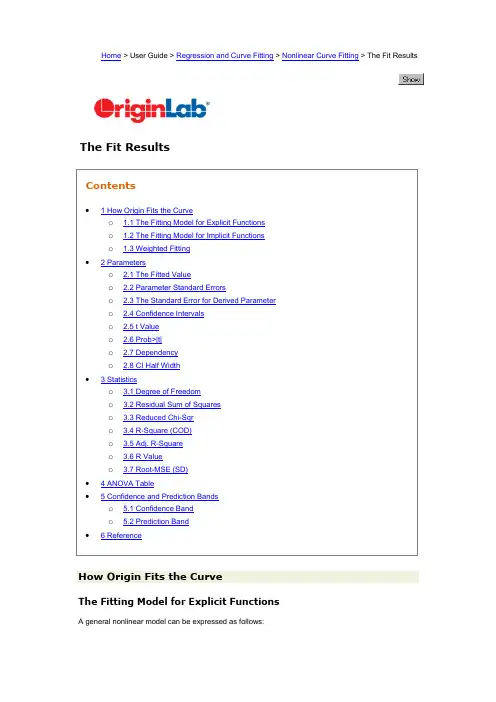
Home > User Guide > Regression and Curve Fitting > Nonlinear Curve Fitting > The Fit ResultsThe Fit ResultsHow Origin Fits the CurveThe Fitting Model for Explicit FunctionsA general nonlinear model can be expressed as follows:(1) where is the independent variables andis the parameters.The aim of nonlinear fitting is to estimate the parameter values which best describe the data. The standard way of finding the best fit is to choose the parameters that would minimize the deviations of the theoretical curve(s) from the experimental points. This method is also called chi-square minimization, defined as follows:(2)where is the row vector for the i th (i = 1, 2, ... , n) observation.To estimate the value with the least square method, we need to solve the normal equations which are set to be zero for the partial derivatives of with respect to each .(3)Since there are no explicit solutions to the normal equations, we employ an iterative strategy to estimate the parameter values. This process starts with some initial values, . With each iteration, avalue is computed and then the parameter values are adjusted to reduce the . When the values computed in two successive iterations are small enough (compared with the tolerance), we can say that the fitting procedure has converged. In the NLFit output messages, you can see the reduced chi-square, which is the mean deviation for all data points, as shown below:(4)Origin uses the Levenberg-Marquardt (L-M) algorithm to adjust the parameter values in the iterative procedure. This algorithm, which combines the Gauss-Newton method and the steepest descent method, works for most cases. You may wish to consult other sources for details of the L-M algorithm. Origin's fitter additionally offers the Simplex method and orthogonal distance regression algorithm.The Fitting Model for Implicit FunctionsA general implicit function could be expressed as:(5)where and are the variables, β are the fitting parameters and const is a constant.The fitting is performed with the ORD Algorithm to minimize the residual sum of squares by adjusting both fitting parameters and values of the independent variable in the iterative process.Weighted FittingWhen the measurement errors are unknown, are set to 1 for all i, and the curve fitting is performed without weighting. However, when the experimental errors are known, we can treat these errors as weights and use weighted fitting. In this case, the chi-square can be written as:(6)There are a number of weighting methods available in Origin. Please read Fitting with Errors and Weighting in the Origin Help file for more details.ParametersThe fit-related formulas are summarized here:The Fitted ValueComputing the fitted values in nonlinear regression is an iterative procedure. You can read a brief introduction in the above section (How Origin Fits the Curve), or see the below-referenced material for more detailed information.Parameter Standard ErrorsDuring L-M iteration, we need to calculate the partial derivatives matrix F, whose element in i th row and j th column is:(7)Then we can get the Variance-Covariance Matrix for parameters by:(8)where s2 is the mean residual variance, or the Deviation of the Model, and can be calculated as follows:(9)The square root of a main diagonal value of this matrix is the Standard Error of the corresponding parameter(10)where C ii is the element in i th row and i th column of the matrix C. C ij is the covariance between θi and θj.You can choose whether to exclude s2 when calculating the covariance matrix. This will affect the Standard Error values. When excluding s2, clear the Use reduce Chi-Sqr check box on the Advanced page. The covariance is then calculated by:(11)So the Standard Error now becomes:(12)The parameter standard errors can give us an idea of the precision of the fitted values. Typically, the magnitude of the standard error values should be lower than the fitted values. If the standard error values are much greater than the fitted values, the fitting model may be overparameterized.The Standard Error for Derived ParameterOrigin estimates the standard errors for the derived parameters according to the Error Propagation formula, which is an approximate formula.Let be the function with a combination (linear or non-linear) of variables .The general law of error propagation is:where is the covariance value for , and.For example, using three variableswe get:Now, let the derived parameter be , and let the fitting parameters be . The standard error for the derived parameter is .Confidence IntervalsOne assumption in regression analysis is that data is normally distributed, so we can use the standard error values to construct the Parameter Confidence Intervals. For a given significance level, α, the (1-α)x100% confidence interval for the parameter is:(13)The parameter confidence interval indicates how likely the interval is to contain the true value.The confidence interval illustrated above is Asymptotic, which is the most frequently used method to calculate the confidence interval. The "Asymptotic" here means it is an approximate value. If you need more accurate values, you can use the Model Comparison Based method to estimate the confidence interval in the Advanced page.If the Model Comparison method is used, the upper and lower confidence limits will be calculated by searching for the values of each parameter p that makes RSS(θj) (minimized over the remaining parameters) greater than RSS by a factor of (1+F/(n-p)).(14)where F = Ftable(α,1,n-p)and RSS is the minimum residual sum of square found during the fitting session.t ValueYou can choose to perform a t-test on each parameter to see whether its value is equal to 0. The null hypothesis of the t-test on the j th parameter is:And the alternative hypothesis is:The t-value can be computed as:(15)Prob>|t|The probability that H0 in the t test above is true.(16)where tcdf(t, df) computes the lower tail probability for Student's t distribution with df degree of freedom.DependencyIf the equation is overparameterized, there will be mutual dependency between parameters. The dependency for the i th parameter is defined as:(17)and (C-1)ii is the (i, i)th diagonal element of the inverse of matrix C. If this value is close to 1, there is strong dependency.CI Half WidthThe Confidence Interval Half Width is:(18)where UCL and LCL is the Upper Confidence Interval and Lower Confidence Interval, respectively. StatisticsSeveral fit statistics formulas are summarized below:Degree of FreedomThe Error degree of freedom. Please refer to the ANOVA Table for more details.Residual Sum of SquaresThe residual sum of squares:(19)Reduced Chi-SqrThe Reduced Chi-square value, which equals the residual sum of square divided by the degree of freedom.(20)R-Square (COD)The R2 value shows the goodness of a fit, and can be computed by:(21)where TSS is the total sum of square, and RSS is the residual sum of square.Adj. R-SquareThe adjusted R2 value:(22)R ValueThe R value is the square root of R2:(23)For more information on R2, adjusted R2 and R, please see Goodness of Fit.Root-MSE (SD)Root mean square of the error, or the Standard Deviation of the model, equal to the square root of reduced χ2:(24)ANOVA TableThe ANOVA Table:Note: In nonlinear fitting, Origin outputs both corrected and uncorrected total sum of squares: Corrected model:(25)Uncorrected model:(26)Confidence and Prediction BandsConfidence BandThe confidence interval for the fitting function says how good your estimate of the value of the fitting function is at particular values of the independent variables. You can claim with 100α% confidence that the correct value for the fitting function lies within the confidence interval, where α is the desired level of confidence. This defined confidence interval for the fitting function is computed as:(27)where:(28) Prediction BandThe prediction interval for the desired confidence level α is the interval within which 100α% of all the experimental points in a series of repeated measurements are expected to fall at particular values of the independent variables. This defined prediction interval for the fitting function is computed as:(29)Reference1. William. H. Press, etc. Numerical Recipes in C++. Cambridge University Press, 2002.2. Norman R. Draper, Harry Smith. Applied Regression Analysis, Third Edition. John Wiley & Sons,Inc. 1998.3. George Casella, et al. Applied Regression Analysis: A Research Tool, Second Edition.Springer-Verlag New York, Inc. 1998.4. G. A. F. Seber, C. J. Wild. Nonlinear Regression. John Wiley & Sons, Inc. 2003.5. David A. Ratkowsky. Handbook of Nonlinear Regression Models. Marcel Dekker, Inc. 1990.6. Douglas M. Bates, Donald G. Watts. Nonlinear Regression Analysis & Its Applications. John Wiley& Sons, Inc. 1988.7. Marko Ledvij. Curve Fitting Made Easy. The Industrial Physicist. Apr./May 2003. 9:24-27.。

循证医学名词术语中英文对照循证医学名词术语中英文对照安全性Safety半随机对照试验quasi- randomized control trial，qRCT背景问题background questions比值比odds ratio，OR标准化均数差standardized mean difference, SMD病例报告case report病例分析case analysis病人价值观patient value病人预期事件发生率patient’s expected event rate, PEER补充替代医学complementary and alternative medicine, CAM 不良事件adverse event不确定性uncertaintyCochrane图书馆Cochrane Library, CLCochrane系统评价Cochrane systematic review, CSR Cochrane协作网Cochrane Collaboration, CCCox比例风险模型Cox’ proportional hazard model参考试验偏倚References test bias肠激惹综合征irritable bowel syndrome，IRB测量变异measurement variation成本-效果cost-effectiveness成本-效果分析cost-effectiveness analysis成本-效益分析cost-benefit analysis成本-效用分析cost-utility analysis成本最小化分析（最小成本分析）cost-minimization analysis重复发表偏倚Multiple publication bias传统医学Traditional Medicine，TMD—L法DerSimonian & Laird methodthe number needed to harm one more patients from the therapy，NNH 对抗疗法allopathic medicine，AM对照组中某事件的发生率control event rate，CER多重发表偏倚multiple publication bias二次研究secondary studies二次研究证据secondary research evidence发表偏倚publication biasnumber needed to treat，NNT非随机同期对照试验non-randomized concurrent control trial 分层随机化stratified randomization分类变量categorical variable风险（危险度）risk干扰co-intervention工作偏倚Workup bias固定效应模型fixed effect model国际临床流行病学网International Clinical Epidemiology Network, INCLEN灰色文献grey literature后效评价reevaluation获益benefit机会结chance node疾病谱偏倚Spectrum bias技术特性Technical properties加权均数差weighted mean difference, WMD 假阳性率（误诊率）false positive rate假阴性率（漏诊率）false negative rate简单随机化simple randomization检索策略search strategy交叉对照研究（交叉设计）crossover design 经济学分析economic analysis经济学特性Economic attributes or impacts经验医学empirical medicine精确性precision决策结decision node决策树分析decision tree analysis绝对获益增加率absolute benefit increase, ABI 绝对危险度降低率absolute risk reduction, ARR 绝对危险度增加率absolute risk increase, ARI 可重复性repeatability，reproducibility可靠性（信度）reliability可信区间confidence interval ，CI可信限confidence limit ，CLLogistic回归模型Logistic regression model历史性对照研究historical control trial利弊比likelihood of being helped vs harmed, LHH连续性变量continuous variable临床对照试验controlled clinical trial, CCT临床结局clinical outcome临床经济学clinical economics临床决策分析clinical decision analysis临床流行病学clinical epidemiology, CE临床实践指南clinical practice guidelines, CPG临床试验clinical trial临床研究证据clinical research evidence临床证据clinical evidence临床证据手册handbook of clinical evidence零点Zero time灵活性flexibility临界点Cut off points漏斗图funnel plots率差（或危险差）rate difference，risk difference，RDMeta-分析Meta-analysis敏感度sensitivity敏感性分析sensitivity analysis墨克手册Merck manual脑卒中病房Stroke Unit内在真实性internal validity偏倚bias起始队列inception cohort前-后对照研究before-after study前景问题foreground questions区组随机化block randomization散点图scatter plots森林图forest plots伤残调整寿命年disability adjusted life year，DALY 生存曲线survival curves生存时间survival time生存质量（生活质量）quality of life世界卫生组织World Health Organization, WHO失安全数fail-Safe Number试验组某事件发生率experimental event rate，EER 似然比likelihood Ratio, LR适用性applicability受试者工作特征曲线（ROC曲线）receiver operator characteristic curve 随机对照临床试验randomized clinical trials, RCT随机对照试验randomized control trial, RCT随机化隐藏randomization concealment随机效应模型random effect model特异度specificity同行评价colleague evaluation统计效能（把握度）power同质性检验tests for homogeneity外在真实性external validity完成治疗分析per protocol，PP腕管综合征carpal tunnel syndrome, CTS卫生技术health technology卫生技术评估health technology assessment, HTA系统评价systematic review, SR相对获益增加率relative benefit increase, RBI相对危险度relative risk，RR相对危险度降低率relative risk reduction, RRR相对危险度增加率relative risk increase, RRI效果effectiveness效力efficacy效应尺度effect magnitude效应量effect size序贯试验sequential trial选择性偏倚selection bias循证儿科学evidence-based pediatrics循证妇产科学evidence-based gynecology & obstetrics 循证购买evidence-based purchasing循证护理evidence-based nursing循证决策evidence-based decision-making循证内科学evidence-based internal medicine循证筛选evidence-based selection循证外科学evidence-based surgery循证卫生保健evidence-based health care循证诊断evidence-based diagnosis循证医学evidence-based medicine, EBM亚组分析subgroup analysis严格评价critical appraisal验后比post-test odds验后概率post-test probability验前比pre-test odds验前概率pre-test probability阳性预测值positive predictive value原始研究primary studies异质性检验tests for heterogeneity意向治疗分析intention-to-treat, ITT阴性预测值negative predictive value引用偏倚citation bias尤登指数Youden’s index语言偏倚language bias预后prognosis预后因素prognostic factor预后指数prognostic index原始研究证据primary research evidence原始研究证据来源primary resources沾染contamination真实性（效度）validity诊断参照标准reference standard of diagnosis。

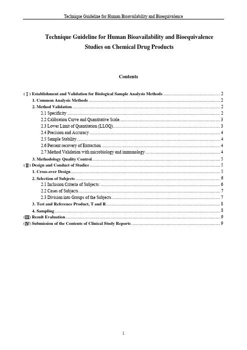
Technique Guideline for Human Bioavailability and BioequivalenceStudies on Chemical Drug ProductsContents(Ⅰ) Establishment and Validation for Biological Sample Analysis Methods (2)1. Common Analysis Methods (2)2. Method Validation (2)2.1 Specificity (2)2.2 Calibration Curve and Quantitative Scale (3)2.3 Lower Limit of Quantitation (LLOQ) (3)2.4 Precision and Accuracy (4)2.5 Sample Stability (4)2.6 Percent recovery of Extraction (4)2.7 Method Validation with microbiology and immunology (4)3. Methodology Quality Control (5)(Ⅱ) Design and Conduct of Studies (5)1. Cross-over Design (5)2. Selection of Subjects (6)2.1 Inclusion Criteria of Subjects: (6)2.2 Cases of Subjects (7)2.3 Division into Groups of the Subjects (7)3. Test and Reference Product, T and R (8)4. Sampling (8)(Ⅲ) Result Evaluation (9)(Ⅳ) Submission of the Contents of Clinical Study Reports (9)Technique Guideline for Human Bioavailability and BioequivalenceStudies on Chemical Drug ProductsSpecific Requirements for BA and BE Studies(Ⅰ) Establishment and Validation for Biological Sample Analysis MethodsBiological samples generally come from the whole blood, serum, plasma, urine or other tissues. These samples have the characteristics such as little quantity for sampling, low drug concentration, much interference from endogenous substances, and great discrepancies between individuals. Therefore, according to the structure, biological medium and prospective concentration scale of the analytes, it is necessary to establish the proper quantitative assay methods for biological samples and to validate such methods.1. Common Analysis MethodsCommonly used analysis methods at present are as follows: (1) Chromatography: Gas Chromatography(GS), High Performance Liquid Chromatography (HPLC), Chromatography－mass Spectrometry (LC-MS, LC-MS-MS, GC-MS, GC-MS-MS), and so on. All the methods above can be used in detecting most of drugs; (2) Immunology methods: radiate immune analysis, enzyme immune analysis, fluorescent immune analysis and so on, all these can detect protein and polypeptide; (3) Microbiological methods: used in detecting antibiotic drug.Feasible and sensitive methods should be selected for biologic sample analysis as far as possible.2. Method ValidationEstablishment of reliable and reproducible quantitative assay methods is one of the keys to bioequivalence study. In order to ensure the method reliable, it is necessary to validate the method entirely and the following aspects should be generally inspected:2.1 SpecificityIt is the ability that the analysis method has to detect the analytes exactly and exclusively, when interference ingredient exists in the sample. Evidences should be provided that the analytes are the primary forms or specific active metabolites of the test drugs. Endogenous instances, the relevant metabolites and degradation products in biologic samples should not interfere with the detection of samples. If there are several analytes, each should be ensured not to be interfered, and the optimal detecting conditions of the analysis method should be maintained. As for chromatography, at least 6 samples from different subjects, which include chromatogram of blank biological samples, chromatogram of blank biologic samples added control substance (concentration labeled) and chromatogram of biologic samples after the administration should beexamined to reflect the specificity of the analytical procedure. As for mass spectra (LC-MS andLC-MS-MS) based on soft ionization, the medium effect such as ion suppression should be considered during analytic process.2.2 Calibration Curve and Quantitative ScaleCalibration curve reflects the relationship between the analyte concentration and the equipment response value and it is usually evaluated by the regression equation obtained from regression analysis (such as the weighted least squares method). The linear equation and correlation coefficient of the calibration curve should be provided to illustrate the degree of their linear correlation. The concentration scale of calibration curves is the quantitative scale. The examined results of concentration in the quantitative scale should reach the required precision and accuracy in the experiment.Dispensing calibration samples should use the same biological medium as that for analyte, and the respective calibration curve should be prepared for different biological samples. The number of calibration concentration points for establishing calibration curve lies on the possible concentration scale of the analyte and on the properties of relationship of analyte/response value. At least 6 concentration points should be used to establish calibration curve, more concentration points are needed as for non-linear correlation. The quantitative scale should cover the whole concentration scale of biological samples and should not use extrapolation out of the quantitative scale to calculate concentrations of the analyte. Calibration curve establishment should be accompanied with blank biologic samples. But this point is only for evaluating interference and not used for calculating. When the warp* between the measured value and the labeled value of each concentration point on the calibration curve is within the acceptable scale, the curve is determined to be eligible. The acceptable scale is usually prescribed that the warp of minimum concentration point is within ±20% while others within ±15%. Only the eligible calibration curve can be carried out for the quantitative calculation of clinical samples. When linear scale is somewhat broad, the weighted method is recommended to calculate the calibration curve in order to obtain a more exact value for low concentration points. ( *: warp=[(measured value － labeled value)/labeled value]×100%)2.3 Lower Limit of Quantitation (LLOQ)Lower limit of quntitation is the lowest concentration point on the calibration curve, indicating the lowest drug concentration in the tested sample, which meets the requirements of accuracy and precision. LLOQ should be able to detect drug concentrations of samples in 3~5 eliminationhalf-life or detect the drug concentration which is 1/10~/20 of the C max. The accuracy of the detection should be within 80~120% of the real concentration and its RSD should be less than 20%. The conclusions should be validated by the results from at least 5 standard samples.2.4 Precision and AccuracyPrecision is, under the specific analysis conditions, the dispersive degree of a series of the detection data from the samples with the same concentration and in the same medium. Usually, the RSD from inter- or intra- batches of the quality control samples is applied to examine the precision of the method. Generally speaking, the RSD should be less than 15% and that around LLOQ should be less than 20%. Accuracy is the contiguous degree between the tested and the real concentrations of the biological samples (namely, the warp between the tested and the real concentrations of the quality-controlled samples). The accuracy can be obtained by repeatedly detecting the analysis samples of known concentration which should be within 85~115% and which around LLOQ should be within 80~120%.Generally, 3 quality-control samples with high, middle and low concentrations are selected for validating the precision and accuracy of the method. The low concentration is chosen within three times of LLOQ, the high one is close to the upper limit of the calibration curve, and the middle concentration is within the low and the high ones. When the precision of the intra-batches is detected, each concentration should be prepared and detected at least 5 samples. In order to obtain the precision of inter-batches, at least 3 qualified analytical batches, 45 samples should be consecutively prepared and detected in different days.2.5 Sample StabilityAccording to specific instances, as for biological samples containing drugs, their stabilities should be examined under different conditions such as the room temperature, freezing, thaw and at different preservation time, in order to ensure the suitable store conditions and preservation times. Another thing that should be paid attention to is that the stabilities of the stock solution and the analyte in the solution after being treated with, should also be examined to ensure the accuracy and reproducibility of the test results.2.6 Percent recovery of ExtractionThe recovery of extraction is the ratio between the responsive value of the analytes recovered from the biological samples and that of the standard, which has the same meaning as the ratio of the analytes extracted from the biologic samples to be analyzed. The recovery of extraction of the 3 concentrations at high, middle and low should be examined and their results should be precise and reproduceable.2.7 Method Validation with microbiology and immunologyThe analysis method validation above mainly aims at chromatography, with many parameters and principles also applicable for microbiological and immunological analysis. However, some special aspects should be considered in the method validation. The calibration curve of the microbiological and immunological analysis is non-linear essentially, so more concentration pointsshould be used to construct the calibration curve than the chemical analysis. The accuracy of the results is the key factor and if repetitive detection can improve the accuracy, the same procedures should be taken in the method validation and the unknown sample detection.3. Methodology Quality ControlThe unknown samples are detected only after the method validation for analysis of biological samples has been completed. The quality control should be carried out during the concentration detection of the biological samples in order to ensure the reliability of the method in the practical application. It is recommended to assess the method by preparing quality-control samples of different concentrations by isolated individuals.Each unknown sample is usually detected for only one time and redetected if necessary. In the bioequivalence experiments, biological samples from the same individual had better to be detected in the same batch. The new calibration curve should be established when detecting biological samples of each analysis batch and high, middle and low concentrations of the quality-control samples should be detected at the same time. Each concentration should at least have two samples and should be equally distributed in the detection sequence of the unknown samples. When there are a large number of unknown samples in one analysis batch, the number of the quality-control samples at different concentrations should be increased to make the quality-control samples exceed 5% of the unknown sample population. The warp of detection result from the quality-control samples should usually be less than 15%, while the warp of the low concentration point should be less than 20% and at most 1/3 results of the quality-control samples at different concentrations are allowed to exceed the limit. If the detection results of the quality-control samples do not accord with the above requirements, the detection results of the samples in this analysis batch should be blanked out.The samples with concentrations higher than the upper quantitation limit should be detected once more using corresponding diluted blank medium. As for those samples with concentrations lower than the lower quantitation limit, during pharmacokinetics analysis, those sampled before reaching C max should be calculated as zero while those after C max should be calculated as ND (Not detectable), so as to decrease the effect of the zero value on the AUG calculation.(Ⅱ) Design and Conduct of Studies1. Cross-over DesignCurrently, the crossover design is the most wildly applied method in the BE study. As for the drug absorption and clearance, there is a transparent variation among individuals. Therefore, the coefficient of variability among individuals is far greater than that of the individual himself. That is why the bioequivalence study is generally required to be designed on the principle of self crossover control. Subjects are randomly divided into several groups and treated in sequence, of whichsubjects in one group take the test products first and then the reference product, while subjects in the other take the reference products first and then the test products. A long enough interval is essential between the two sequences, which is called Wash-out period. In this way, every subject has been treated twice or more times sequentially, which is equal to self-control. Therefore, the influence of drug products on drug absorption can be discriminated from the others, and the effect of various test periods and individual difference on the results can be eliminated.Two-sequence crossover design, three-sequence crossover design are adopted respectively according to the amount of the test product. If two varieties of drug products are to be compared, the two-treatment, two-period or two-sequence crossover design will be a preferable choice. When three varieties of products (two test products and one reference product) are included, thethree-formulation, three-period and double 3×3 Latin square design will be the suitable choice. And a long enough wash-out period is required among respective periods.Wash-out period is set on purpose to eliminate the mutual disturbance of the two varieties of drug products and avoid the treatment in the prior period from affecting that of the next period. And the wash-out period is generally longer than or equal to 7 elimination half lives.While the half-lives of some drugs or their active metabolites are too long, it is not suitable to apply the crossover design. Under this circumstance, parallel design is adopted, but the sample size should be enlarged.However, as for some highly variable drugs, except for increase of the subjects, repetitive cross-over design can be applied, to test possibly existing difference in individual when receive the same preparation twice.2. Selection of Subjects2.1 Inclusion Criteria of Subjects:The difference among individuals of the subjects should be minimized so that the difference of the drug products can be detected. The inclusion criteria and exclusion criteria should be noted in the trial scheme.Male healthy subjects are recruited generally. And as to the drugs of special purpose, proper subjects are recruited according to specific conditions. If female healthy subjects are recruited, the possibility of gestation should be avoided. If the drugs to be tested have some known adverse effects, which may do harm to the subjects, patients can also be included as the subjects.Age: 18~ 40 years old generally. The difference in age of the subjects in one batch should not be more than 10 years.Body weight: not less than 50kg as to normal subjects. Body Mass Index (BMI), which is equal to body weight (kg)/ body height 2 (m2), is generally required to be in the range of standard body weight. For the subjects in one batch, the taken dosage is the same, the range of the bodyweight, therefore, should not have great disparity.The subjects should receive the overall physical examination and be proved healthy. There is not medical history of heart, kidney, digestive tract, nervous system, mental anomaly, metabolism dysfunction, and so on. The physical examination has revealed normal blood pressure, heart rate, electrocardiogram, and respiratory rate. Laboratory data have revealed normal hepatic function, renal function and blood function. Those examinations are essential to prevent the metabolism of drugs in vivo from being interfered by the diseases. According to the classification and safety of drugs, special items examinations are required before, during and after the test, such as the blood glucose examination, which is required in the drug trial of hypoglyceimic agents.In order to avoid the interference by other drugs, no administration of other drugs is allowed from two weeks before and till the end of the test. Moreover, the cigarette, wine,beverage with caffeine, or some fruit juice that may affect the metabolism of the drug, is forbidden during the trial period also. The subjects had better have no appetite of cigarette and wine. Possible effects of the cigarette-addicted history should not be neglected in the discussion of results.Due to the metabolism variance resulted by known genetic polymorphism of drugs, the safety factor which may be effected by the slow metabolism speed of drugs should be considered.2.2 Cases of SubjectsThe cases of the subjects should meet the statistic requirement. And according to the current statistical methods, 18~24 cases are enough for most drugs to meet the requirement of sample size. But as to some drugs of high variability, more cases may be required correspondingly.The cases of a clinic trial are determined by three fundamental factors: （1）Significance level: namely, the value of α, for which value 0.05 or 5% is often adopted;（2）Power of a test: namely, the value of 1-β. β is the index that represents the probability of the type error, which is also theⅡprobability of misjudging the actually efficacy drugs as inefficient drugs, and value not less than 80% is commonly stated; （3）Coefficient of variance（CV%）and Difference（θ）: In the equivalence test of two drugs, the greater CV% and θ of the test indexes are, the more cases are required. The CV% and θ are unknown before the trial and can only be estimated by the above parameters of the owned reference products or running the preliminary test. Moreover, when a BA test has been finished, the value of N can be calculated according to the parameters such as θ, CV% and 1-β and then compared with the cases adopted in the finished BA test to determine whether the cases are reasonable or not.2.3 Division into Groups of the SubjectsThe subjects should be randomly divided into different comparable groups. The cases of the two groups should guarantee the best comparability.3. Test and Reference Product, T and RThe quality of the reference products directly affect the results reliability of BE trial. Generally, the domestic innovator products of the same dosage form which has been approval to be on sale are commonly selected. If it failed in acquiring the innovator products, the key product on the market can also be chosen as the reference product and the related quality certifications (such as the test results of the assay and dissolution) and the reasons for option should be provided. When it comes to the drug study of specific purpose, other on-sale dosage forms which are of the same kind and similar with pharmaceutics properties are selected as the reference products and those reference products should be already on sale and qualified in quality. The difference in assay between the test product and reference product should not exceed 5%.The test product should be the scale-up product or manufacture scale product, which is consistent with the quality standards for clinical application. And the indexes such as the in vitro dissolution, stability, content or valence assay, consistency reports between batches should be provided to the test unit for reference. As for some drugs, the data of polymorphs and optical isomers should be offered additionally. The test and reference product should be noted with the advanced development unit, batch number, specification, storage conditions and expiry date.For future reference, the test and reference product should be kept long enough after the trialtill the product is approved to be on sale.4. SamplingThere is a significant sense in designing the sampling point to guarantee both the reliability of the trial results and the rationality of calculating the pharmacokinetics parameters. Commonly, there should be preliminary tests or the pharmacokinetics literatures at home and abroad served as the evidences of designing the reasonable sampling points. When the blood-drug concentration assay is performed, the absorption phase, balance phase and clearance phase should be considered overall. There must be enough sampling points in every phase of the C-T curve and around the T max. The concentration curve, therefore, can fully reflect the entire procedure of the drugs distribution in vivo. And the blank blood samples are taken before the administration. Then at least 2~3 points are sampled in the absorption phase, at least 3points are sampled near the C max and 3-5 points in the clearance phase. Try to avoid that the first point gets the C max, and running the preliminary test may avoid this. When the continuously-sampling results show that the drugs’ primary forms or the active metabolites are at the point of 3～5 half- lives or the blood drug concentration is 1/10～1/20 ofC max, the values of AUC0-t/AUC0-∞are generally bigger than 80% .For the terminal clearance item doesn’t affect the evaluation of the products’ absorption process much, as to the long half-life drugs, the sampling periods should be continued long enough, so that the whole absorption process can be compared and analyzed. In the multiple administration study, the BA of some drugs is known to beaffected by the circadian rhythm, samples of which should be taken 24 hours continuously if possible.When the BA of the test drugs can’t be determined by detecting the blood-drug concentration, if the primary forms and the active metabolites of the test drugs are mainly be excreted in urine (more than 70% of the dosage), the BA assay may be performed by detecting the urine drug concentration, which is the test of the accumulated excretion quantity of drugs in urine to reflect the intake of drugs. The test products and trial scheme should accord with the demands of BA assay. The urine samples should be collected at intervals, and the collection frequency and intervals of which should meet the demands of evaluating the excretion degree of the primary forms and the active metabolites of the test products in urine. However this method cannot reflect the absorption speed of the drugs and gets many error factors, it is not recommended generally.Some drugs metabolize so rapidly in vivo that it is impossible to detect the primary forms in biological samples. Under these circumstances, the method determining the concentration of corresponding active metabolites in biological samples is adopted to perform the BA and BE studies.(Ⅲ) Result EvaluationAt present, the weighting function of AUC on drug absorption degree is comparatively affirmed, while C max and T max sometimes are not sensitive and seemly enough for weighting the absorption speed due to their dependence on the arrangement of sampling time, and they are therefore not suitable for drug products with multi-peak phenomena and for experiments with large individual variation. During the evaluation, if there are some special instances of inequivalence, a specific analysis should be performed for specific problems.As for AUC，the 90% confidence interval is generally required within the scope of 80%~125%. As for the drugs with narrow treatment spectrum, the above scope should likely be appropriately reduced. While in a few instances, having been validated to be reasonable, the scope can also be increased. So does C max. And as for T max, statistical evaluation is required only when its release speed is closely correlated to clinical therapeutic effects and safety, the equivalence scope of which can be ascertained according to the clinical requirements.When bioavailability ratio of test products is higher than that of reference products, which is called suprabioavailability, the following two instances can be considered: 1). Whether the reference product itself is a product with low bioavailability, which results in the improvement of the test drug's bioavailability; 2). The quality of the reference product meets the requirement, and the test drug really has higher bioavailability.(Ⅳ) Submission of the Contents of Clinical Study ReportsIn order to satisfy the demand of evaluation, a clinical report of bioequivalence study shouldinclude the following contents: (1)Experiment subjective;(2) Establishment of analysis methods for bioavailability samples and data of inspection, as well as provision of the essential chromatograms;(3) Detailed experiment design and operation methods , including data of all the subjects，sample cases，reference products，given dosage，usage and arrangement of sampling time;(4) All data about original measurement of unknown sample concentrations，pharmacokinetics parameters and drug-time curve of each subjects;(5) Data handling procedure and statistical analysis methods as well as detailed procedure and results of statistics;(6) Observation results of clinical adverse reactions after taking medicine，midway exit and out of record of subjects and the reasons;(7) Result analysis and necessary discussion on bioavailability or bioequivalence; (8) References. A brief abstract is required before the main body; at the end of the main body, names of the experiment unit, chief persons of the study and experiment personnel should be signed to take the responsibility for the results of the study.。

Technical ReportPigment Selection Using Kubelka–Munk Turbid Media Theory and Non-Negative Least Square TechniqueSummer 2004Mahnaz MohammadiMahdi NezamabadiLawrence A. TaplinRoy S. BernsSpectral Color Imaging Laboratory GroupMunsell Color Science LaboratoryChester F. Carlson Center for Imaging ScienceRochester Institute of Technologymm0252@, mxn9911@, taplin@,berns@/Abstract - This report describes a process of pigment selection for reconstructing the Gamblin Conservation Colors and various artist pigments dispersed in linseed oil. Single constant Kubelka–Munk (K-M) turbid media theory and a non-negative least square (NNLS) optimization technique were employed in this experiment. Eleven pigments were selected as representative of the 30-pigments Gamblin Conservation Colors. These were quinacridone red (PV 19), venetian red (PR 101), cadmium red medium (PR 108), cadmium yellow medium (PY 37), indian yellow (PY 83), chromium oxide green (PG 17), phthalocyanine green (PG 7), phthalocyanine blue (PB 15:2), cobalt blue (PB 28), titanium dioxide white (PW 6), and ivory black (PBK 9).The report is classified into four sections:A.Preparing the samples and spectral measurementsB.Pigment characterizationC.Color matching and pigment selectionD.Verification of selected pigments with unknown samplesA.Preparing the samples and spectral measurementsAll samples in this study were prepared from the Gamblin Conservation Colors. The 30 pigments were grouped into three sets, chromatic, earth, and achromatic, shown in Table I. These paints were made from aldehyde resin (Laropal A81), petroleum distillate mixture, and lightfast pigments. Most of them are transparent or semi transparent. More details can be found on the Gamblin webside, .Since the masstone of an individual pigment is dark, it is difficult to determine its characteristic absorption bands. Therefore pigments were characterized relative to one particular spectrally–nonselective pigment. In this experiment each pigment was mixedwith a white pigment (TiO2) at two different ratios. The formulations are summarized inTable I in Appendix B. Titanium white is a highly reflective and scattering pigment so by adding it to the other pigments it is possible to make an opaque film. Figures 1-3 show spectral reflectance spectra of the three groups of Gamblin colors. The measurements were performed using a GretagMacbeth SpectroEye with 45/0 geometry measuring in the wavelength range from 380 to 730 nm in intervals of 10 nm with a 4.5 mm circular aperture.Table I. Gamblin Conservation Colors used in K/S building process.Pigment name Chemical name ColorIndexnumberViridian Hydrated chromium oxide PG 18Ultramarine blue Complex silicate of sodium & aluminum with sulfur PB 29Quinacridone red Quinocridone red b PV 19Prussian blue Ferri-ammonium ferrocyanide PB 27:1Phthalo green Chlorinated copper phthalocyanine PG 7Phthalo blue Copper phthalocyanine PB 15:2Dioxazine purple Carbazol dioxazine PV 23Hansa Yellow Medium Arylide yelow PY 74Cadmium Orange Concentrated cadmium sulfo-selenide PO 20Manganese blue Hue Copper phthalocyanine PB 15:4Cadmium Yellow Light Concentrated cadmium zinc sulfide PY 35Cadmium Yellow Medium Concentrated cadmium sulfide PY 37Chromium Oxide Green Chromium oxide green PG 17Cobalt blue Oxides of cobalt & aluminum PB 28Cobalt Green Oxides of cobalt & zinc PG 19Cobalt Violet Cobalt phosphate PV 14Indian Yellow Diarylide yellow HR70PY 83Cadmium Red Light Concentrated cadmium sulfo-selenide PR 108c h r o m a t i c Cadmium Red Medium Concentrated cadmium sulfo-selenide PR 108Venetian Red Synthethic red iron oxide PR 101Transparent Earth Yellow Transparent Mars yellowPY 42Transparent Earth Red Transparent Mars red PR 101Raw Umber Natural iron oxide containing manganese PBr 7Yellow Ocher Natural hydrated iron oxide PY 43Indian Red Synthetic red iron oxide PR 101Burnt Sienna Calcinated natural iron oxide PBr 7Burnt Umber Natural iron oxide containing manganese PBr 7e a r t h Raw Sienna Natural iron oxide PBr 7Titanium White Titanium dioxide PW 6Ivory Black Bone black PBk 9a c h r o m a t i c Black Spinel Copper chromite black spinel PBk 28Figure 1a. Spectral reflectance and logarithm [1/(K/S)] of Gamblin chromatic colors.Figure 1b. Spectral reflectance and logarithm [1/(K/S)] of Gamblin chromatic colors.Figure 1c. Spectral reflectance and logarithm [1/(K/S)] of Gamblin chromatic colors.Figure 2a. Spectral reflectance and logarithm [1/(K/S)] of Gamblin earth colors.Figure 2b. Spectral reflectance and logarithm [1/(K/S)] of Gamblin earth colors.Figure 2c. Spectral reflectance and logarithm [1/(K/S)] of Gamblin earth colors.Figure 3. Spectral reflectance and logarithm [1/(K/S)] of blacks and white (TiO 2).Since spectral reflectance at lower wavelengths was not so precise due to noisy data in this range of spectrum, these data were truncated to avoid differential absorption of TiO 2versus the other pigment ; hence all calculations were performed between 430-730 nm.Matlab 5.2 was used as a toolbox for all calculations.B. Pigment characterizationKubelka-Munk turbid media theory is a practical theory for the prediction of the relationship between pigment concentration and spectral reflectance of paint films [1-3].In this research, it was assumed that the samples were opaque and the opacity was related to the white pigment (TiO 2). Therefore the single constant K-M theory was employed for pigment characterization and pigment selection and the following equations were used: R l ,mix=1+K S Ê Ë Á ˆ ¯ ˜ l ,mix -K S Ê Ë Á ˆ ¯ ˜ l ,mix 2+2K S Ê Ë Á ˆ ¯ ˜ l ,mix È Î Í ˘ ˚ ˙ 12(1)whereK S Ê Ë Á ˆ ¯ ˜ l ,mix =C i k s Ê Ë Á ˆ ¯ ˜ i =1n Âl ,i (2)and R l ,mix is the spectral reflectance factor of a mixture, K S ()l ,mix is the spectralabsorption (K) and scattering (S) ratio of a mixture, k s ()l ,i is the unit k s ()of a pigment,C i is the amount of a pigment, and n is the number of pigments in a mixture. By having K S ()l ,mix properties of a mixture of the colored pigment and white at knownconcentrations, unit k s ()l ,i for all pigments were calculated using Eq. (2). In order to have a curve shape independent of concentration for the pigments, log 1K S ()[] was calculated [1]. Since log 1K S ()[] was plotted, the maximum corresponds to the maximum of the reflectance curve. This is a ‘’signature’’ of a pigment and it can be determined how the spectral characteristics of the pigments in each group are similar or dissimilar with each other. Of course it should be noted that the unit k s () values at each wavelength are specific for the particular vehicle system and white pigment used [8]. The log 1K S ()[] spectra of each pigment are plotted in Figures 1-3. For example, cobalt blue has a very characteristic spectrum. It exhibits a sharp rise in reflectance in the red region and has a slight band in the middle of the spectrum. The cobalt blue has characteristic curve shape in the region of maximum reflectance that would be another clue for identification of this special pigment. Chromium oxide green, sometimes called Vert Emeraude Dull, is known since the early nineteenth century [8]. The double absorption bands at 465 nm and 600 nm of the pure chrome oxide are characteristic of this pigment.Since yellows absorb in the short-wavelength violet region and reflect almost all wavelengths, there is no minimal absorption characteristic for these pigments. The flatness in the absorption region of cadmium reds is characteristic. Reflectance of cadmium red light rises at a shorter wavelength than cadmium red medium. Quinacridone red is categorized as violet pigment in color index. It’s two or more absorption bands are specific to quinacridone red. Earth pigments do not have characteristic absorption bands that are as well defined as chromatic pigments.B. Color matching and pigment selectionIn this part of experiment, each sample of the Gamblin database (60 samples) was used as a target and it was hypothesized that the target is a combination of the pigments in the database:K S Ê Ë Á ˆ ¯ ˜ l ,unknown -k s Ê Ë Á ˆ ¯ ˜ l ,white È Î Í ˘ ˚ ˙ =C i k s Ê Ë Á ˆ ¯ ˜ j =1n Âl ,j(3)Equation (3) can be written using statistical notation [4].Y i =b 1X i ,1+b 2X i ,2+...b n X i ,n (4)where the independent variable, X i ,n , represent the unit k s () of a pigment in which i represents wavelength, Y is the dependent variable and represents the K S properties of the unknown mixture minus unit k s () of white, and b n represents the pigment amounts.The constraint of having non-negative concentration was also considered in the regression (NNLS). The above equations can be shown using vector-matrix notation:b =¢ X X()-1¢ X Y (5)whereb =C 1C 2..C n È Î Í Í Í Í Í Í ˘ ˚ ˙ ˙ ˙ ˙ ˙ ˙ ,X =k s Ê Ë Á ˆ ¯ ˜ l 430,1...k s Ê Ë Á ˆ ¯ ˜ l 430,n ............k s Ê Ë Á ˆ ¯ ˜ l 730,1...k s Ê Ë Á ˆ ¯ ˜ l 730,n È Î Í Í Í Í Í Í Í Í ˘ ˚˙ ˙ ˙ ˙ ˙ ˙ ˙ ˙ andY =K S Ê Ë Á ˆ ¯ ˜ l 430,unknown -k s Ê Ë Á ˆ ¯˜ l 430,w ...K S Ê Ë Á ˆ ¯ ˜ l 730,unknown -k s Ê Ë Á ˆ ¯ ˜ l 730,w È ÎÍ Í Í Í Í Í Í Í ˘ ˚ ˙ ˙ ˙ ˙ ˙ ˙ ˙ ˙ If the unknown is metameric, minimizing K S ()differences does not minimize either reflectance differences or visual differences [1]. A weighting function, d l , can be introduced to improve correlation [11].d l =∂R l ,unknown ∂K S Ê Ë Á ˆ ¯ ˜ l ,unknown =-2R 2l ,unknown K S Ê Ë Á ˆ ¯ ˜ l ,unknown1-R 2l ,unknown ()(6)All the spectral data in equation (5) were premultiplied by the weighting function. This led to differences in weighted K S () being better correlated with differences in spectral reflectance factor.All three, four, and five combinations of thirty pigments were made computationally:n r Ê Ë Á ˆ ¯ ˜ =n !n -r ()!r !(7)Therefore 303Ê Ë Á ˆ ¯ ˜ =4,060, 304Ê Ë Á ˆ ¯ ˜ =27,405, and 305Ê Ë Á ˆ ¯˜ =142,506 recipe were generated,respectively. It should be noted that white pigment was included in all recipes and it was assumed that the total amount of material is 1+C i i =1n ÂÊ Ë Á ˆ ¯˜ . This means that the amount of white pigment was set equal by one and the amount of the other pigments were added up.Every recipe was employed to predict all the chromatic and earth Gamblin samples. Sincethere is no single metric that can express the accuracy of spectral matching, a group of metrics was used. These included:1. Spectral difference, root mean square error (RMS).2. Color difference, D E00D65,2o ().3. Metamerism index(MI00D65ÆA (),4. GFC metric.Details of these metrics are presented in Appendix A.It should be noted that the earth and chromatic pigments were analyzed separately. The results of the predicted samples were rearranged in ascending order and the top thirty recipes were selected for further analysis. It was not guaranteed that the first recipe was the best one.C.1. Color gamut evaluationThe range of colors produced by a coloration system is called its color gamut [1]. In this experiment the coloration system is a set of pigments. The volume of a color solid was calculated using corrected CIELAB values based on the CIE94 color difference equation, similar to Luo’s LLAB [7]. The color gamuts of the first thirty sets were calculated. For each pigment a logarithmic range of concentration (between zero and one) at seven levels was designed. For each set, the full factorial of seven levels of concentrations was considered. It should be noted that white pigment was always included in a recipe. Therefore 74=2,401, 75=16,807, 76=117,649points in CIELAB color space were generated as concentrations for 3-pigment, 4-pigment, and 5-pigment recipes, respectively. By having unit k s() of the pigments and the generated concentrations, the spectral reflectance of each recipe was synthesized. The corrected CIELAB wascalculated using equations (8), designated by L94,a94, and b94. These values comprise athree dimensional solid that is the color gamut in CIE94 corrected CIELAB space:L94=L*C94=ln1+0.045C* ()0.045h 94=arctan b*a*()a 94=C94cos h94()b 94=C94sin h94()(8)Outer shells of the generated color gamut were found using the ‘’convhulln’’ function in matlab and the corresponding volume generated by the pigments were saved. A set from the first thirty top recipes with larger color gamut was selected as the best recipe at each error criterion. The same procedure was performed for chromatic and earth pigments. The results are tabulated in Tables II and III.Table II-Three, four, and five- pigment sets based on the spectral matching of chromaticsamples using different criteria.3-pigment setsRMS (%)D E00GFC MI00 pigment 1Cadmium red medium Cadmium red medium Indian yellow Indian yellow pigment 2Hansa yellow medium Hansa yellow medium Phthalocyanine green Phthalocyanine green pigment 3Phthalocyanine blue Ultramarine blue Dioxazine purple Dioxazine purple Volume563075227656975569754-pigment setspigment 1Quinacridone red Cadmium red medium Quinacridone red Quinacridone red pigment 2Indian yellow Hansa yellow medium Hansa yellow medium Indian yellow pigment 3Phthalocyanine green Phthalocyanine green Phthalocyanine green Phthalocyanine green pigment 4Cobalt blue Cobalt blue Cobalt blue Cobalt blueVolume714057766073147714055-pigment setspigment 1Quinacridone red Cadmium red medium Cadmium red medium Cadmium red medium pigment 2Cadmium yellow medium Cadmium orange Hansa yellow medium Indian yellow pigment 3Phthalocyanine green Hansa yellow medium Phthalocyanine green Phthalocyanine green pigment 4Manganese blue hue Phthalocyanine green Manganese blue hue Cobalt blue pigment 5Cobalt blue Cobalt blue Cobalt blue Ultramarine blue Volume71238804017924880601The projection of three-dimensional color spaces for the selected pigments ontoa 94b94axes at different L94levels is shown in Figures 4a-4d.Figure 4a.b94 versus a94at different L94levels for three, four, and five-pigment recipesbased on the spectral matching of chromatic samples using RMS criterion. Red lines indicate 3-pigment set, green lines indicate 4-pigment set, and blue lines indicate 5-pigment set.Figure 4b.b94 versus a94at different L94levels for three, four, and five-pigmentrecipes based on the spectral matching of chromatic samples using D E00 criterion. Red lines indicate 3-pigment set, green lines indicate 4-pigment set, and blue lines indicate 5-pigment set.Figure 4c.b94 versus a94at different L94levels for three, four, and five-pigment recipesbased on the spectral matching of chromatic samples using GFC criterion. Red lines indicate 3-pigment set, green lines indicate 4-pigment set, and blue lines indicate 5-pigment set.Figure 4d.b94 versus a94at different L94levels for three, four, and five-pigment recipesbased on the spectral matching of chromatic samples using MI00D65ÆA()criterion.Red lines indicate 3-pigment set, green lines indicate 4-pigment set, and blue lines indicate 5-pigment set.As can be seen from the above figures and tables, adding one pigment to the system from three to four made a significant improvement in color gamut at all error criteria. Movingfrom four pigments to five does not have the same improvement effect as moving from three to four pigments. The selected pigments at the different criteria are not exactly the same but the generated color gamuts almost have the same range of volume for three, four, and five pigments. The area size of slices of color gamuts depends on the pigmentsused in generating the color solid. In this study, for the case of pigments selected basedon RMS criterion, the area corresponding to the three pigments is larger than areas offour and five pigments. Color gamut of the selected pigments for matching the earth pigments was also calculated and shown in Figures 5a-5d and Table III.Table III. Three, four, and five-pigment sets based on the spectral matching of earth samples using different criteria.3-pigment setsRMS (%)D E00GFC MI00 pigment 1Venetian red Cadmium red medium Venetian red Venetian red pigment 2Indian yellow Indian yellow Indian yellow Indian yellow pigment 3Prussian blue Phthalocyanine green Prussian blue Manganese blue hue Volume377024562437702243624-pigment setspigment 1Indian red Indian red Indian red Quinacridone red pigment 2Cadmium red light Cadmium red light Trans. Earth red Yellow ocher pigment 3Yellow ocher Indian yellow Indian yellow Manganese blue hue pigment 4Prussian blue Phthalocyanine green Prussian blue Cobalt blueVolume276494759840502317365-pigment setspigment 1Quinacridone red Quinacridone red Quinacridone red Cadmium red medium pigment 2Trans. Earth red Cadmium orange Trans. Earth red Trans. Earth red pigment 3Yellow ocher Cadmium yellow light Yellow ocher Cadmium orange pigment 4Black spinel Phthalocyanine green Black spinel Manganese blue hue pigment 5Ultramarine blue Cobalt violet Ultramarine blue Ultramarine blue Volume37482735123748241005Figure 5a.b94 versus a94at different L94levels for three, four, and five-pigment recipesbased on the spectral matching for earth samples using RMS criterion. Red lines indicate 3-pigment set, green lines indicate 4- pigment set, and blue lines indicate 5-pigment set.Figure 5b.b94 versus a94at different L94levels for three, four, and five-pigment recipesbased on the spectral matching for earth samples using D E00 criterion. Red lines indicate3-pigment set, green lines indicate 4-pigment set, and blue lines indicate 5-pigment set.Figure 5c.b94 versus a94at different L94levels for three, four, and five-pigment recipesbased on the spectral matching of earth samples using GFC criterion. Red lines indicate 3-pigment set, green lines indicate 4-pigment set, and blue lines indicate 5-pigment set.Figure 5d. b94 versus a94at different L94levels for three, four, and five-pigment recipesbased on the spectral matching of earth samples using MI00D65ÆA() criterion. Redlines indicate 3-pigment set, green lines indicate 4-pigment set, and blue lines indicate 5-pigment set.As can be seen from the Tables II and III and Figure 4-5, in most cases the volume of color solid generated by the sets for matching the earth pigments were smaller than the corresponding volumes in the chromatic pigments. In the cases that chromatic pigments were used in predicting the earth samples, the color gamut gets larger than those sets containing only earth pigments. Therefore having a large color gamut is highly dependent on the selected pigments and not just on to the number of pigments in the set. It means that three chromatic pigments can make a larger color gamut than four earth pigments.In order to investigate which pigments have more influence on making a larger color gamut, the volume of generated color gamut using the first thirty top sets was calculated and plotted against the corresponding error criterion (Figures 6a-6d). As can be seen,some plots in Figure 6 are clustered into two groups. The sets corresponds to each group was investigated and it was found that those sets containing phthalocyanine green make the color gamut significantly bigger than the other sets and the top clusters contain this pigment.(a)(b)( c )(d)Figure 6. Volume of color gamut generated by the first thirty top sets sorted in different error criteria: a) spectral RMS, b) D E 00, c) GFC, d) MI 00D 65ÆA (). Blue lines indicate 3-pigment sets, red lines indicate 4-pigment sets, and yellow lines indicate 5-pigment sets .The performance of spectral matching of chromatic and earth samples using the selected set of pigments based on different error criteria is summarized in Tables IV and V, respectively.Table IV. Statistical results of performance of predicting the chromatic samples.Results Three-pigment Four- Pigment Five-PigmentRMS (%)Average10.6 6.5 4.4Minimum0.10.10.0Maximum42.616.713.5Standard Deviation10.1 5.2 4.2D E00Average11.2 6.8 4.6Minimum0.10.10.0Maximum32.924.818.6Standard Deviation9.2 6.9 5.6GFCAverage0.96820.98470.9915Minimum0.89910.93140.9615Maximum 1.0000 1.0000 1.0000Standard Deviation0.02960.01760.0100MI00D65ÆA ()Average 1.30.80.6 Minimum0.00.00.0 Maxiumum 5.0 3.9 2.6 Standard Deviation 1.50.80.6The average performance of 10.6% spectral RMS and 11.2 D E00of 3-pigment sets arelarge enough to convince one that three pigments could not be sufficient for spectral matching. The average performance of 1.3 metamerism is not so high but the associatedD E00 are in the range of 8 to 17 D E00, which are high. In other words, the prediction errordoes not change so much under different illumination. Since the associated D E00 is largethe average prediction error would be large for other illumination. Hence small average metamerism index is not an indication of good color matching unless it is associated withthe small average D E00.The spectral plots of measured and predicted chromatic Gamblin samples using the selected sets based on spectral RMS are shown in Figures 7-11. In most cases the three-pigment set could not match the pigments well and at least the shape were not the same as original except in those cases that the target pigment was one of the pigments of the selected set. Four and five-pigment set could take the pattern of the original shape and they are almost acceptable but not as a perfect spectral matching.Figure 7. Spectral reflectance of green pigments using the sets sorted based on RMS. Green lines indicate using 3-pigment set, red lines indicate using 4-pigment set, cyan lines indicate using 5-pigment set, and blue lines indicate the measured spectral reflectance.Figure 8. Spectral reflectance of blue pigments using the sets sorted based on RMS. Green lines indicate using 3-pigment set, red lines indicate using 4-pigment set, cyan lines indicate using 5-pigment set, and blue lines indicate the measured spectral reflectance.Figure 9. Spectral reflectance of red pigments using the sets sorted based on RMS. Green lines indicate using 3-pigment set, red lines indicate using 4-pigment set, cyan linesindicate using 5-pigment set, and blue lines indicate the measured spectral reflectance.Figure 10. Spectral reflectance of yellow pigments using the sets sorted based on RMS. Green lines indicate using 3-pigment set, red lines indicate using 4-pigment set, cyan lines indicate using 5-pigment set, and blue lines indicate the measured spectralreflectance.Figure 11. Spectral reflectance of violet pigments using the sets sorted based on RMS. Green lines indicate using 3-pigment set, red lines indicate using 4-pigment set, cyan lines indicate using 5-pigment set, and blue lines indicate the measured spectral reflectance.The lower averages of spectral RMS, D E00, and higher average of GFC indices for theprediction of earth pigments indicates better spectral matching performance than for chromatic samples. The five-pigment recipes have reasonably small averages. The performances of predictions are improved by moving from three to four and then to five pigments. Again, there is greater improvement from three to four pigments than from four to five pigments. The performance of spectral matching of earth samples using the selected set of pigments based on different error criteria is summarized in Table V.The spectral plots of measured and predicted earth Gamblin samples using the selected sets based on spectral RMS are shown in Figures 12-14. In most cases all three, four, and five pigments could match the pigments very well and they are almost acceptable. Therefore in order to reduce the number of pigments in the set, the set containing three pigments was selected as the best set of pigments for matching earth samples.Table V. Statistical results of performance of predicting the earth samples.Results Three-pigment Four- Pigment Five-PigmentRMS (%)Average 1.30.70.4Minimum0.00.00.1Maximum 2.9 2.4 1.5Standard Deviation0.80.70.4D E00Average 2.3 1.10.5Minimum0.60.00.1Maximum 6.5 2.8 1.3Standard Deviation 1.60.70.3GFCAverage0.99880.99960.9999 Minimum0.99480.99910.9993 Maximum 1.0000 1.0000 1.0000 Standard Deviation0.00140.00030.0002MI00D65ÆA ()Average0.20.10.1Minimum0.00.00.0Maximum0.40.40.1Standard Deviation0.10.10.0Figure 12. Spectral reflectance of brown pigments using the sets sorted based on RMS. Green lines indicate using 3-pigment set, red lines indicate using 4-pigment set, cyan lines indicate using 5-pigment set, and blue lines indicate the measured spectral reflectance.Figure 13. Spectral reflectance of red earth pigments using the sets sorted based on RMS. Green lines indicate using 3-pigment set, red lines indicate using 4-pigment set, cyan lines indicate using 5-pigment set, and blue lines indicate the measured spectral reflectance.Figure 14. Spectral reflectance of yellow earths pigments using the sets sorted based on RMS. Green lines indicate using 3-pigment set, red lines indicate using 4-pigment set, cyan lines indicate using 5-pigment set, and blue lines indicate the measured spectral reflectance.As a conclusion, the five-pigment sets had better performance for predicting the chromatic samples and three-pigment sets were sufficient for predicting the earth samplesat different criteria. Therefore a data set containing eight pigments could be a representative of Gamblin Conservation Colors. Since RMS optimization was employed for predicting the samples, the selected three earth and five chromatic pigments based on this criteria (Table VI) were chose as the selected set. The spectral plots of the pigments included in the selected set are shown in Figure 15.Table VI. Selected pigments based on spectral RMS optimizationPigment #Pigment name1Quinacridone red2Cadmium yellow medium3Phthalocyanine green4Manganese blue hue5Cobalt blue6Venetian red7Indian yellow8Prussian blueFigure 15. Spectral reflectance of the selected pigments based on RMS criterion.D. Verification of selected pigments with unknown samplesIn this part of the experiment the quality of the selected set based on RMS criteria of part C was examined. Several verification targets were selected. The first was Matisse’s Pot of Geraniums, an oil painting on linen painted by Henri Matisse in 1912. The second was four panels of painted patches contain 64, 61, 32, and 64 oil painted patches, respectively. Since there were some repeated samples in the Matisse group so the 15 samples of them were selected as the verification target. Patches of panels were made of mixing a coloredpigment with TiO2 dispersed in poly-vinyl acetate (PVA). The samples prepared at NGAby painting conservation department. The measurements were performed using spectroEye measuring in the wavelength range from 380 nm to 730 nm in interval of 10 nm. The CIELAB colorimetric attributes were also calculated for the targets using D65 illuminant and 2O observer. The verification targets, their spectral reflectance factors and color distribution are shown in Figures 16-20.。

ICH 安全性领域常用专业术语中英文对照表S9-mix constituent S9混合液成分Safeguards 安全监测Safety pharmacology 安全药理学Safety margin 安全范围Salmonella typhimurium 鼠伤寒沙门菌Sampling time 采样时间Satellite groups 卫星组Saturation of absorption 吸收饱和Secondary testing 二期试验Secretion in milk 乳汁分泌Sensitive periods 敏感期Sensitivity 敏感性Sensory functions and reflexes 感觉功能和反射Sexual maturity 性成熟Short term toxicity 短期毒性Short or medium-term carcinogenicity study 短或中期致癌性研究Short treatment 短期处理Sighting studies 预试验Single dose(acute)toxicity 单剂量(急性)毒性Single study design 单一研究设计Site-specific targeted delivery 定位靶向释放Small colony 小集落Small colony mutant 小集落突变体Soft agar method 软琼脂法Soluble genotoxic impurity 可溶性遗传毒性杂质Solvent control 溶剂对照Somatic cell 体细胞Somatic cell test 体细胞试验Species 种属Specificity 特异性Species specificity 种属特异性Sperm analysis 精子分析Sperm count 精子计数Sperm maturation 精子成熟Sperm morphology 精子形态学Sperm motility 精子活动度Sperm viability 精子活力Spermatogenesis 精子形成Spindle apparatus 纺缍体Stages of reproduction 生殖阶段Standard battery of test 标准试验组合Standard 3-test battery 标准三项试验组合Standard battery 标准组合Standard battery system 标准组合系统Standard procedure 标准规程Standard protocol 标准试验方案Standard set of strains 标准菌株组Standard set of tests 标准试验组Standard test battery 标准试验组合Statistical evaluation 统计学评价Steady-state levels 稳态浓度Step-by-step 逐步Stepwise process 阶梯式程序Strain 品系Structural changes 结构改变Structural chromosomal aberration 染色体结构畸变Subgroups 亚组Supravital staining 体外活动染色Surface righting reflex 平面翻正反射Survival 存活率suspension 悬浮物Systemic exposure 全面接触Target organs 靶器官Target cell 靶细胞Target histidine genes 组氨酸目的基因Target tissue 靶组织Target tissue exposure 靶组织接触Teratogenic response 致畸胎反应Terminal sacrifice 终末期处死Test of carcinogenicity 致癌试验Test approach 试验方法Test battery approach 试验组合方法Test compound 受试物Test model 试验模型Test strategy 试验策略Test systems 试验系统Tester strain 试验菌株Therapeutic 治疗Therapeutic confirmatory 疗效确定Therapeutic exploratory 疗效探索Therapeutic indication 治疗适应证Time course 时程Timing conventions 分段计时方法Tissue cross-reactivity 组织交叉反应Tissue distribution 组织分布Tissue exposure 组织接触Tissue uptake 组织吸收Tk locus tk位点Top concentration 最高浓度Topical 局部的Topoisomerase inhibitor 拓朴异构酶抑制剂Total erythrocyte 总红细胞Total litter loss 整窝丢失Toxicity to reproduction 生殖毒性Toxicokinetics 毒代动力学(毒物代谢动力学) Transgene 转基因Transgenic animals 转基因动物Transgenic plants 转基因植物Translocation 移位Treatment regimen 实施方案Tubal transport 输卵管运输Tumor induction 肿瘤诱导Tumor response 肿瘤反应Tumor-related gene 肿瘤相关基因Two or three phase approach 分段(二段或三段)研究Two study design 分段(两段)研究设计Ovulation rate 排卵率Unbound concentration 未结合浓度Unexpected finding 非预期结果Unscheduled DNA synthesis(UDS) 程序外DNA合成Unstable epoxide 不稳定过氧代物Vaginal opening 阴道张开Vaginal plug 阴栓Whole blood 全血Dead offspring at birth 出生时死亡的子代Degradation 降解Delay of parturition 分娩延迟Deletion 缺失Descriptive statistics 描述性统计Detection of bacterial mutagen 细菌诱变剂检测Detection of clastogen 染色体断裂剂检测Determination of metabolites 测定代谢产物Development of the offspring 子代发育Developmental toxicity 发育毒性Diminution of the background lawn 背景减少Direct genetic damage 直接遗传损伤Distribution 分布DNA adduct DNA加合物DNA damage DNA损伤DNA repair DNA修复DNA strand breaks DNA链断裂Dose escalation 剂量递增Dose dependence 剂量依赖关系Dose level 剂量水平Dose-limiting toxicity 剂量限制性毒性Dose-raging studies 剂量范围研究Dose-relatived mutagenicity 剂量相关性诱变性Dose-related 剂量相关Dose-relatived cytotoxicity 剂量相关性细胞毒性Dose-relatived genotoxic activity 剂量相关性遗传毒性Dose-response curve 剂量-反应曲线Dosing route 给药途径Duration 周期Duration of pregnancy 妊娠周期Eaning 断奶Earlier physical malformation 早期躯体畸形Early embryonic development 早期胚胎发育Early embryonic development to implantation 着床早期的胚胎发育Electro ejaculation 电射精Elimination 清除Embryofetal deaths 胚胎和胎仔死亡Embryo-fetal development 胚胎-胎仔发育Embryo-fetal toxicity 胚胎-胎仔毒性Embryonic death 胚胎死亡Embryonic development 胚胎发育Embryonic period 胚胎期Embryos 胚胎Embryotoxicity 胚胎毒性Enantiomer 对映异构体End of pregnancy 怀孕终止Endocytic 内吞噬(胞饮)Endocytic activity 内吞噬活性Endogenous proteins 内源性蛋白Endogenous components 内源性物质Endogenous gene 内源性基因Endonuclease 核酸内切酶Emdpmiclease release from lysosomes 溶酶体释放核酸内切酶End-point 终点Epididymal sperm maturation 附睾精子成熟性Epitope 抗原决定部位Error prone repair 易错性修复Escalation 递增Escherichia coli strain 大肠杆菌菌株Escherichia coli 大肠杆菌Evaluation of test result 试验结果评价Exaggerated pharmacological response 超常增强的药理作用Excretion 排泄(清除)Exposure assessment 接触剂量评价Exposure period 接解期External metabolizing system 体外代谢系统F1-animals 子一代动物False positive result 假阳性结果Fecundity 多产Feed-back 反馈Fertilisation 受精Fertility 生育力Fertility studies 生育力研究Fetal abnormalities 胎仔异常Fetal and neonatal parameters 胎仔和仔鼠的生长发育参数Fetal development and growth 肿仔发育和生长Fetal period 胎仔期Fetotoxicity 胎仔毒性False negative result 假阴性结果First pass testing 一期试验Fluorescence in situ hybridization(FISH) 原位荧光分子杂交Foetuses 胎仔Formulation 制剂Frameshift mutation 移码突变Frameshite point mutation 移码点突变Free-standing 独立Fresh dissection technique 新鲜切片技术Funtional deficits 切能缺陷Functional test 功能试验Functional indices 功能性指标Fusion proteins 融合蛋白Gametes 配子Gender of animals 动物性别Gender-specific drug 性别专一性药物Gene knockout 基因剔除Gene therapy 基因治疗Gene mutation 基因突变Genetic 遗传Genetic change 遗传学改变Genetic damage 遗传学损伤Genetic endpoint 遗传终点Genetic toxicity 遗传毒性Genotoxic activity 遗传毒性作用Genotoxic carcinogen 遗传毒性致癌剂Genotoxic effect 遗传毒性效应Genotoxic hazard 遗传毒性危害Genotoxic potential 潜在遗传毒性Genotoxic rodent carcinogen 啮齿类动物遗传毒性致癌剂Genotoxicity 遗传毒性Genotoxicity test 遗传毒性试验Genotoxicity test battery 毒性试验组合Genotoxycity evaluation 遗传毒性评价Germ cell mutagen 生殖细胞诱变剂Germ line mutation 生殖系统突变GLP 临床前研究质量管理规范Gross chromosomal damage 染色体大损伤Gross evaluation of placenta 胎盘的大体评价Growth factors 生长因子Haemotoxylin staining 苏木素染色Half-life 半衰期Hematopoietic cells 造血细胞Heptachlor 七氯化合物Heritable 遗传Heritable defect 遗传缺陷Heritable disease 遗传性疾病Heritable effect 遗传效应High concentration 高浓度Histologic appearance of reproductive organ 生殖器官的组织学表现Histopathological chang 组织病理学改变Homologous proteins 同系蛋白Homologous series 同系Host cell 宿主细胞Human subjects 人体Human carcinogen 人类致癌剂Human lymphoblastoid TH6cell 人成淋巴TK6细胞Human mutagen 人类致突变剂Humoral immunity 体液免疫Immature erythrocyte 未成熟红细胞Immediate and latent effect 速发和迟发效应Immunogenicity 免疫原性Immunopathological effects 免疫病理反应immunotoxicity 免疫毒性Implantation 着床Implantation sites 着床部位In vitro 体外In vitro test 体外试验In vivo 体内In vivo test 体风试验Incidence of polyploidy cell 多倍体细胞发生率Incisor eruption 门齿萌发Independent test 独立试验Individual fetal body weight 单个胎仔体重Induced and spontaneous models of disease 诱发或自发的疾病模型Inducer of micronuclei 微核诱导剂Inhalation 吸入Inhibitor of DNA metabolism DNA代谢抑制剂Intact animals 完整动物(整体动物)Internal control 内对照Interphase nuclei 分裂间期细胞核Intra-and inter-individual 个体与个体间Isolated organs 离休器官Juvenile animal studies 未成年动物研究Kinetic profile 动力学特点Kinetics 动力学Lactation 授乳、哺乳Large deletion event 大缺失事件Late embryo loss 后期胚胎丢失Level of safety 安全水平Libido 性欲Life threatering 危及生命Lipophilic compound 亲脂性化合物Litter size 每窝胎仔数目Live and deal conceptuese 活胎和死胎Live offspring at birth 出生时存活的子代Local tolerance studies 局部耐受性研究Local toxicity 局部毒性Locu 位点Long-term carcinogenicity study 长期致癌性研究Loss of the tk gene tk基因缺失Major organ formation 主要器官形成Male fertility 雄性生育力Male fertility assessment 雄性生育力评价Mammalian sells 哺乳动物细胞Mammalian species 哺乳类动物Mammalian sell mutation test 哺乳动物细胞致突变试验Marketing approval 上市许可Maternal animal 亲代动物Mating behavior 交配行为Mating period 交配期Mating ratio 交配比例Matrices 基质Maximum tolerated dose(MTD) 最大耐受剂量Mechanism of genotoxicity 遗传毒性机制Mechanistic investigation 机制研究Metabolic activation 代谢活化Metabolic activation pathway 代谢活化途径Metabolic activation system 代谢活化系统Metabolism 代谢Metabolites profile 代谢物的概况Metaphase 中期Metaphase analysis 分裂中期相分析Metaphase cell 分裂中期相细胞Micronucleus 微核Micronucleus formation 微核形成Microtitre 微滴定Mictotitre method 微滴定法mimicking 模拟Mitotic index 有丝分裂指数Molecular characterization 分子特性Molecular technique 分子技术Monitor 监测Monoclonal antibodies 单克隆抗体Non-toxic compound 无毒化合物Mouse lymphoma L5178Y cell 小鼠淋巴瘤L5178Y细胞Mouse lymphoma tk assay 小鼠淋巴溜tk检测Mutagen 诱变原Mutagenic carcinogen 诱变性致癌剂Mutagenic potential of chemical 化合物的潜在致突变性Mutant colony 突变体集落Mutation 突变Mutation induction in transgenes 转基因诱导突变Naked eye 肉眼Necropsy(macroscopic examination) 解剖(大体检查)Negative control 阴性对照Negative result 阴性结果Neonate adaptation to extrauterine life 新生仔宫外生活的适应性Newborn 新生仔Newcleated 有核Non rodent 非啮齿类Non-clinical 非临床Non-genotoxic carcinogen 非遗传毒性致癌剂Non-genotoxic mechanism 非遗传毒性机制Non-human primate 非人灵长类Non-linear 非线性No-toxic-effect dose level 无毒性反应剂量水平Nucleated bone marrow cell 有核骨髓细胞Nucleoside analogue 核苷酸同系物Number of live and dead implantation 宫内活胎和死胎数Numerical chromosomal aberration 染色体数目畸变Numerical chromosome changes 染色体数目改变Oestrous cycle 动情周期Oligonucleotide grugs 寡核苷酸药物One ,twe,three generation studies 一、二、三子代研究Organ development 器官发育Paraffine embedding 石蜡包埋Parameter 参数Parent compound 母体化合物Parenteral 非肠道Particulate material 颗粒物Parturition 分娩Pediatric populations 小儿人群Peproductive competence 生殖能力Peripheral blood erythrocyte 外周血红细胞Pharmacodynamic effects 药效作用Pharmacodynamics 药效学(药效动力学) Pharmacokinetic 药代动力学Phenylene diamine 苯二胺Physical development 身体发育Physiological stress 生理应激Pilot studies 前期研究Pinna unfolding 耳廓张开Plasmid 质粒Plasminogen activators 纤维蛋白溶解酶原激活因子Ploidy 整倍体Point mutation 点突变Polychromatic erythrocyte 嗜多染色红细胞Polycyclic hydrocarbon 多环芳烃Polymer 聚合物Polyploidy cell 多倍体细胞Polyploidy 多倍体Polyploidy induction 多倍体诱导Poorly soluble compound 难溶化合物Positive control 阳性对照Positive result 阳性结果Post meiotic stages 减数分裂后期Post-approval 批准后Postcoital time frame 交配后日期Postimplantation deaths 着床后死亡Postnatal deaths 出生后死亡Postweaning development and growth 断奶后发育和生长Potential 潜在性Potential immunogenecity 潜在免疫原性Potential target organs for toxicity 潜在毒性靶器官Pre-and post-natal development study 围产期的发育研究Pre-and postweaning survival and growth 断奶前后的存少和生长Precipitate 沉淀期Precision 精密度Preclinical safety evaluation 临床前安全性评价Predetermined criteria 预定标准Prediction of carcinogenicity 致癌性预测Pregnant 怀孕Pregnant and lactation animals 怀孕与哺乳期动物Preimplantation stages of the embryo 胚胎着床前期Preimplantation development 着床前发育Preliminary studies 预试验Premating 交配前Premating treatment 交配前给药Pre-screening 预筛选Prevalence of abnormalities 异常情况的普遍程度Preweaning 断奶前Primary active entity 主要活性实体Priority selection 优先选择Pro-drug 前体药物Prolongation of parturition 产程延长Protein binding 蛋白结合率Protocol modification 试验方案修改Quantification of mutant 突变体定量Racemate 消旋体Radiolabeled proteins 放射性同位素标记蛋白Radiolabelled compounds 放性性同位素标记化合物Range-finding test 范围确定试验Rate of preimplantation deaths 着床关死亡率Rational study design 合理的试验设计Receptor properties 受体性质Recombinant DNA proteins DNA重组蛋白Recombinant DNA technology DNA重组技术Recombination 重组Recombinant plasma factors 重组血浆因子Reduction in the number of revertants 回复突变数的减少Relative plating efficiency 相对接种效率Relative suspension growth 相对悬浮生长率Relative total growth 相对总生长率Relevant animal species 相关动物种属Relevant dose 相关剂量Relevant factor 相关因素Repeated-dose toxicity studies 重复剂量毒性研究Reproductive function 生殖功能Reproductive toxicity 生殖毒性Reproductive/developmental toxicity 生殖/发育毒性Reverse mutation 回复突变Reversibility 可恢复性(可逆性)Risk assessment 危险度评价Rodent 啮齿类动物Rodent hematopoietic cell 啮齿类动物造血细胞Route of administration 给药途径Routine testing 常规试验S9-mix constituent S9混合液成分Safeguards 安全监测Safety pharmacology 安全药理学Safety margin 安全范围Salmonella typhimurium 鼠伤寒沙门菌Sampling time 采样时间Satellite groups 卫星组Saturation of absorption 吸收饱和Secondary testing 二期试验Secretion in milk 乳汁分泌Sensitive periods 敏感期Sensitivity 敏感性Sensory functions and reflexes 感觉功能和反射Sexual maturity 性成熟Short term toxicity 短期毒性Short or medium-term carcinogenicity study 短或中期致癌性研究Short treatment 短期处理Sighting studies 预试验Single dose(acute)toxicity 单剂量(急性)毒性Single study design 单一研究设计Site-specific targeted delivery 定位靶向释放Small colony 小集落Small colony mutant 小集落突变体Soft agar method 软琼脂法Soluble genotoxic impurity 可溶性遗传毒性杂质Solvent control 溶剂对照Somatic cell 体细胞Somatic cell test 体细胞试验Species 种属Specificity 特异性Species specificity 种属特异性Sperm analysis 精子分析Sperm count 精子计数Sperm maturation 精子成熟Sperm morphology 精子形态学Sperm motility 精子活动度Sperm viability 精子活力Spermatogenesis 精子形成Spindle apparatus 纺缍体Stages of reproduction 生殖阶段Standard battery of test 标准试验组合Standard 3-test battery 标准三项试验组合Standard battery 标准组合Standard battery system 标准组合系统Standard procedure 标准规程Standard protocol 标准试验方案Standard set of strains 标准菌株组Standard set of tests 标准试验组Standard test battery 标准试验组合Statistical evaluation 统计学评价Steady-state levels 稳态浓度Step-by-step 逐步Stepwise process 阶梯式程序Strain 品系Structural changes 结构改变Structural chromosomal aberration 染色体结构畸变Subgroups 亚组Supravital staining 体外活动染色Surface righting reflex 平面翻正反射Survival 存活率suspension 悬浮物Systemic exposure 全面接触Target organs 靶器官Target cell 靶细胞Target histidine genes 组氨酸目的基因Target tissue 靶组织Target tissue exposure 靶组织接触Teratogenic response 致畸胎反应Terminal sacrifice 终末期处死Test of carcinogenicity 致癌试验Test approach 试验方法Test battery approach 试验组合方法Test compound 受试物Test model 试验模型Test strategy 试验策略Test systems 试验系统Tester strain 试验菌株Therapeutic 治疗Therapeutic confirmatory 疗效确定Therapeutic exploratory 疗效探索Therapeutic indication 治疗适应证Time course 时程Timing conventions 分段计时方法Tissue cross-reactivity 组织交叉反应Tissue distribution 组织分布Tissue exposure 组织接触Tissue uptake 组织吸收Tk locus tk位点Top concentration 最高浓度Topical 局部的Topoisomerase inhibitor 拓朴异构酶抑制剂Total erythrocyte 总红细胞Total litter loss 整窝丢失Toxicity to reproduction 生殖毒性Toxicokinetics 毒代动力学(毒物代谢动力学) Transgene 转基因Transgenic animals 转基因动物Transgenic plants 转基因植物Translocation 移位Treatment regimen 实施方案Tubal transport 输卵管运输Tumor induction 肿瘤诱导Tumor response 肿瘤反应Tumor-related gene 肿瘤相关基因Two or three phase approach 分段(二段或三段)研究Two study design 分段(两段)研究设计Ovulation rate 排卵率Unbound concentration 未结合浓度Unexpected finding 非预期结果Unscheduled DNA synthesis(UDS) 程序外DNA合成Unstable epoxide 不稳定过氧代物Vaginal opening 阴道张开Vaginal plug 阴栓Whole blood 全血。

ROC曲线指受试者工作特征曲线/ 接收器操作特性曲线(receiver operating characteristic curve），是反映敏感性和特异性连续变量的综合指标,是用构图法揭示敏感性和特异性的相互关系，它通过将连续变量设定出多个不同的临界值，从而计算出一系列敏感性和特异性，再以敏感性为纵坐标、(1—特异性）为横坐标绘制成曲线，曲线下面积越大，诊断准确性越高。

在ROC曲线上，最靠近坐标图左上方的点为敏感性和特异性均较高的临界值.考虑一个二分问题，即将实例分成正类（positive）或负类(negative)。

对一个二分问题来说，会出现四种情况.如果一个实例是正类并且也被预测成正类，即为真正类（True positive），如果实例是负类被预测成正类,称之为假正类(False positive)。

相应地,如果实例是负类被预测成负类，称之为真负类（True negative）,正类被预测成负类则为假负类(false从列联表引入两个新名词。

其一是真正类率(true positive rate ，TPR）, 计算公式为TPR=TP/ （TP+ FN），刻画的是分类器所识别出的正实例占所有正实例的比例。

另外一个是负正类率(false positive rate, FPR）,计算公式为FPR= FP / （FP + TN），计算的是分类器错认为正类的负实例占所有负实例的比例。

还有一个真负类率（True Negative Rate,TNR），也称为specificity，计算公式为TNR=TN/ (FP+ TN）= 1—FPR.其中，两列True matches和True non-match分别代表应该匹配上和不应该匹配上的两行Pred matches和Pred non-match分别代表预测匹配上和预测不匹配上的在一个二分类模型中,对于所得到的连续结果，假设已确定一个阀值,比如说0.6，大于这个值的实例划归为正类，小于这个值则划到负类中。

英语作文两条曲线范文英文回答：Curves are an enchanting and ubiquitous part of our physical and mathematical world, captivating our imaginations and inspiring scientific breakthroughs. They represent deviations from linearity, revealing the complexities and nuances that enrich our experiences. In mathematics, curves can be defined as graphs of functions, offering a visual manifestation of relationships between variables. The two curves that I find particularly captivating are the parabola and the sine wave, each possessing unique characteristics that have shaped our understanding of the world.Parabolas are quadratic curves that open either upwards or downwards, their shape reminiscent of a graceful arc. They are defined by the equation y = ax^2 + bx + c, where 'a' determines the parabola's orientation and curvature. Parabolas have numerous applications in physics, includingthe trajectory of projectiles and the shape of reflectors used in flashlights and satellite dishes. Their ability to model parabolic motion has been instrumental in advancing our understanding of celestial mechanics and projectile dynamics.Sine waves, on the other hand, are periodic curves that oscillate smoothly between positive and negative values. They are defined by the equation y = Asin(Bx + C), where'A' represents the amplitude, 'B' the frequency, and 'C' the phase shift. Sine waves occur extensively in nature, describing phenomena such as sound waves, electromagnetic waves, and the tides. Their rhythmic patterns have inspired countless applications in signal processing, acoustics, and electronics.The parabola and the sine wave, though vastly different in their equations and shapes, share a common trait: they are both fundamental to our understanding of natural phenomena. Parabolas model the graceful flight of a thrown ball and the focused beam of a flashlight, while sine waves capture the rhythm of sound waves and the rhythmic ebb andflow of the ocean's tides. These curves are not merely mathematical abstractions but powerful tools that have shaped our scientific and technological advancements.中文回答：曲线是物理和数学世界中迷人且普遍存在的一部分，它们吸引着我们的想象力并激发了科学突破。

我们进行临床试验的目的是检验药物（治疗）的效果，而效果往往是需要一个参照药物（治疗）的。

在临床试验中，研究参与人员往往对优效、等效、非劣效这三个概念不是很清晰，甚至对混用，尤其是在根据统计分析结果来推导结论时。

优效性研究假设如下：H0（无效假设，Null Hypothesis）：研究药物疗效—对照药物疗效<优效标准H1（备择假设，Alternative Hypothesis）：研究药物疗效—对照药物疗效=>优效标准当拒绝H0时，统计结论是可以认为研究药物疗效优于对照药物；当不能拒绝H0时，统计结论是不可以认为研究药物疗效优于对照药物。

非劣效性研究假设如下：H0（无效假设，Null Hypothesis）：研究药物疗效—对照药物疗效<非劣效标准H1（备择假设，Alternative Hypothesis）：研究药物疗效—对照药物疗效=>非劣效标准当拒绝H0时，统计结论是可以认为研究药物疗效不劣于对照药物；当不能拒绝H0时，统计结论是不可以认为研究药物疗效不劣于对照药物。

等效性研究假设如下：H0（无效假设，Null Hypothesis）：|研究药物疗效-对照药物疗效|>等效标准H1（备择假设，Alternative Hypothesis）：|研究药物疗效-对照药物疗效|<=等效标准当拒绝H0时，统计结论是可以认为研究药物疗效与对照药物等效；当不能拒绝H0时，统计结论是不可以认为研究药物疗效与对照药物等效。

而我们做的比较多是非等效研究，即当等效标准为0时，与等效性研究假设相反的研究。

假设如下：H0（无效假设，Null Hypothesis）：|研究药物疗效-对照药物疗效|<=等效标准=0H1（备择假设，Alternative Hypothesis）：|研究药物疗效-对照药物疗效|>等效标准=0当拒绝H0时，统计结论是可以认为研究药物疗效与对照药物不等效；当不能拒绝H0时，统计结论是不可以认为研究药物疗效与对照药物不等效（但不是等效）。