Urban Political Economics
- 格式:pdf
- 大小:518.04 KB
- 文档页数:70
地理经济学外国书籍地理经济学是一门研究地理空间与经济活动之间关系的学科。
在这个全球化的时代,地理经济学对于了解国际经济格局和全球化趋势至关重要。
下面介绍几本外国的地理经济学经典著作,帮助读者深入了解这一领域的研究成果。
1. 《地理经济学》(Economic Geography)- Paul Krugman这本书是地理经济学领域的经典之作,作者保罗·克鲁格曼是诺贝尔经济学奖得主。
他通过分析地理空间的重要性以及经济活动对地理环境的影响,揭示了地理经济学的核心理论。
这本书系统阐述了地理经济学的基本概念、方法和应用,涵盖了全球化、城市化、区域发展等重要议题。
2. 《地理经济学导论》(Introduction to Economic Geography)- Danny MacKinnon, Andrew Cumbers这本教材是一本面向学生和研究人员的地理经济学导论。
作者通过案例研究和实证分析,介绍了地理经济学的各个领域,包括产业地理学、城市地理学、区域发展等。
这本书强调了地理空间对经济活动的重要性,帮助读者理解全球经济格局的演变和地理因素的作用。
3. 《经济地理学》(Economic Geography: An Institutional Approach)- Maryann P. Feldman, Dieter F. Kogler这本书从制度经济学的角度分析了经济地理学的核心问题。
作者探讨了制度环境对于经济发展和地理空间的影响,深入研究了创新、产业集群和区域发展等议题。
这本书强调了制度环境对经济活动和地理区域的塑造作用,对于理解经济地理学的制度分析方法具有重要意义。
4. 《城市经济学》(Urban Economics)- Arthur O'Sullivan这本书从经济学的角度研究了城市化和城市经济学的相关问题。
作者分析了城市的特点、城市经济的组织和城市政策的影响等方面。
这本书涵盖了城市空间结构、城市劳动市场、城市土地利用和城市政策等内容,对于理解城市经济学的理论和实证研究具有重要价值。
城市经济学教学大纲一、引言城市经济学是研究城市发展与经济活动之间关系的学科。
本课程将通过理论和实践相结合的方式,系统介绍城市经济学的基本理论框架、研究方法和应用案例,旨在培养学生对城市经济学的理论基础和实践应用的理解和能力。
二、课程目标1. 掌握城市经济学的基本概念和理论框架;2. 理解城市经济发展的影响因素和机制;3. 熟悉城市经济学的研究方法和数据分析技巧;4. 能够分析和解释城市经济现象,并提出合理的政策建议;5. 培养批判性思维和创新能力,为城市经济学领域的研究和实践做出贡献。
三、课程内容1. 城市经济学概述1.1 城市经济学的定义和发展历程1.2 城市经济学的基本假设和理论框架1.3 城市经济学与其他相关学科的关系2. 城市发展理论与模型2.1 都市化与城市化过程的理论解释2.2 博弈论在城市发展中的应用2.3 城市增长模型及其解释力分析3. 城市劳动市场与人口流动3.1 城市劳动力供求关系的分析3.2 人口流动与城市劳动力市场的影响3.3 城市居民收入与福利分析4. 城市地理经济学4.1 城市空间结构与居住选择模型4.2 城市交通与交通拥堵的经济学分析4.3 地区经济发展与区域差异的研究5. 城市政策与规划5.1 城市公共设施和公共服务的供给与需求分析 5.2 城市基础设施建设与可持续发展5.3 城市规划与土地利用的经济学分析四、教学方法本课程将采用多种教学方法,包括课堂讲授、案例分析、小组讨论和实践项目等。
通过课堂讲解,学生将获得城市经济学的基本知识和理论框架;通过案例分析和小组讨论,学生将锻炼批判性思维和解决问题的能力;并通过实践项目,学生将运用所学知识解决实际城市经济问题。
五、考核方式1. 课堂参与和小组讨论:占总成绩的20%2. 期中考试:占总成绩的30%3. 实践项目报告:占总成绩的30%4. 期末考试:占总成绩的20%六、参考教材1. 华东师范大学城市经济学,李华敏,出版社:高等教育出版社2. 城市经济学导论,王小为、张小明,出版社:清华大学出版社3. Urban Economics and Real Estate: Theory and Policy,James C. Vanderbeck and John C. Knight,Publisher: John Wiley & Sons七、参考文献1. Glaeser, E. L., & Gottlieb, J. D. (2009). The Wealth of Cities: Agglomeration Economies and Spatial Equilibrium in the United States. Journal of Economic Literature, 47(4), 983-1028.2. Duranton, G., & Puga, D. (2004). Micro-foundations of Urban Agglomeration Economies. In J. V. Henderson & J-F. Thisse (Eds.), Handbook of Regional and Urban Economics (Vol. 4, pp. 2063-2117). Elsevier.以上即为《城市经济学教学大纲》的内容,本课程将着重培养学生对城市经济学的理论和应用的理解和能力,以期为学生今后在城市发展和经济政策方面的研究和实践提供基础。
英国大学之伦敦政治经济学院伦敦政治经济学院(The London School of Economics and Political Science)简称LSE,是英国最著名的社会科学高等教育机构之一,也是世界一流学府之一。
LSE成立于1895年,其学科涵盖了经济、法律、政治、社会等各个领域。
下面将为大家介绍这所世界一流大学的悠久历史和学术成就。
一、学校历史伦敦政治经济学院的前身为伦敦大学政治经济学学院,成立于1895年。
其前身是,由伦敦大学和伦敦大学学院合并而成的一所学校,其创始人是法国哲学家奥古斯特·孔德。
孔德认为社会科学需要通过不同的视角来探讨,他的观点得到了当时社会上的认可。
在学校创立的初期,该校的教师和学生主要来自欧洲大陆,随着时间的推移,该校的声誉逐渐扩大,吸引了越来越多的国际学生前来学习。
如今,学校有来自全球155个国家的约10000名学生,在国际范围内具有广泛的声誉。
二、学校概况伦敦政治经济学院是世界上最著名的社会科学机构之一,在经济学、政治学、哲学、法律、数学、统计学等领域中,均有出色的表现。
学校主要设有四个学院,包括经济学学院、法学学院、社会科学和公共政策学院、管理学院,并设有更多的分支机构,如欧洲研究中心等。
学校不仅注重学术研究,也非常重视学生的国际性视野和跨学科的研究方法。
学生可以在学校内充分展示自己的想象力与创造力,探索未知领域和研究课题。
三、学校特色伦敦政治经济学院最引人注目也最为独特的特点是,该校广泛使用教育形式的讲座。
这种教学方式在学界非常受欢迎。
学校教员通常会在60分钟左右的时间里讲授一些开放性的问题,以引发学生的思考。
这种方式使学生们不断地进一步了解学科的深度和宽度,从而增强了学生们的学术兴趣和研究能力。
学校鼓励学生参与全球化领域的交流,提供不同的学术论坛,让交流者来自不同的国家和领域。
学校还与全球其他知名大学建立了伙伴关系,为学生提供了国际机会。
四、学校成就伦敦政治经济学院经过100多年的发展,已经成为世界上社科教育领域的领导者之一,在相关领域获得了很高的声誉。
常见的建筑术语中英文对译(2)以下整理了一些常见的建筑术语,中英文对译,以供有需要的朋友使用,仅供参考。
对译集合之二:101. 建筑燃气系统设计- Gas System Design for Buildings102. 建筑消防报警系统设计- Fire Alarm System Design for Buildings103. 建筑智能化系统集成设计- Intelligent System Integration Design for Buildings 104. 建筑幕墙设计- Curtain Wall Design105. 建筑石材幕墙设计- Stone Curtain Wall Design106. 建筑玻璃幕墙设计- Glass Curtain Wall Design107. 建筑绿化设计- Greening Design for Buildings108. 建筑景观设计- Landscape Design for Buildings109. 建筑室内环境设计- Indoor Environmental Design for Buildings110. 建筑声学装修设计- Acoustic Decoration Design for Buildings111. 建筑光学装修设计- Optical Decoration Design for Buildings112. 建筑材料装修设计- Decorative Materials Design for Buildings113. 建筑历史与理论- Architectural History and Theory114. 建筑美学史- History of Architectural Aesthetics115. 现代建筑设计- Modern Architectural Design116. 后现代建筑设计- Postmodern Architectural Design117. 当代建筑设计- Contemporary Architectural Design118. 解构主义建筑设计- Deconstructivist Architectural Design119. 装饰艺术建筑设计- Art Deco Architectural Design120. 功能主义建筑设计- Functionalist Architectural Design121. 结构主义建筑设计- Structuralist Architectural Design122. 新古典主义建筑设计- Neoclassical Architectural Design123. 折衷主义建筑设计- Eclectic Architectural Design124. 绿色建筑设计- Green Architectural Design125. 人文主义建筑设计- Humanist Architectural Design126. 新地域主义建筑设计- New Regionalist Architectural Design 127. 参数化建筑设计- Parametric Architectural Design128. 数字建筑设计- Digital Architectural Design129. 未来主义建筑设计- Futurist Architectural Design130. 智能化建筑设计- Intelligent Building Design131. 生态建筑设计- Ecological Architectural Design132. 城市设计- Urban Design133. 景观设计- Landscape Design134. 城市规划- Urban Planning135. 城市更新- Urban Renewal136. 城市改造- Urban Transformation137. 城市意象- Urban Image138. 城市设计理论- Urban Design Theory139. 城市生态设计- Urban Ecological Design140. 城市交通设计- Urban Transportation Design141. 城市基础设施设计- Urban Infrastructure Design142. 城市天际线设计- Urban Skyline Design143. 城市夜景设计- Urban Nightscape Design144. 城市滨水区设计- Urban Waterfront Design145. 城市开放空间设计- Urban Open Space Design146. 城市街道景观设计- Urban Streetscape Design147. 城市公园设计- Urban Park Design148. 城市居住区设计- Urban Residential District Design149. 城市商业区设计- Urban Commercial District Design150. 城市文化区设计- Urban Cultural District Design151. 城市行政中心设计- Urban Governmental District Design152. 城市会展中心设计- Urban Exhibition and Convention Center Design 153. 城市体育馆设计- Urban Stadium Design154. 城市图书馆设计- Urban Library Design155. 城市博物馆设计- Urban Museum Design156. 城市大剧院设计- Urban Theater Design157. 城市机场设计- Urban Airport Design158. 城市火车站设计- Urban Train Station Design159. 城市地铁站设计- Urban Subway Station Design160. 城市公交车站设计- Urban Bus Stop Design161. 城市景观照明设计- Urban Landscape Lighting Design162. 城市标识系统设计- Urban Signage System Design163. 城市公共艺术装置设计- Public Art Installation Design164. 城市家具设计- Urban Furniture Design165. 城市花坛设计- Urban Flower Bed Design166. 城市儿童游乐设施设计- Urban Playground Design167. 城市植栽设计- Urban Planting Design168. 城市排水系统设计- Urban Drainage System Design169. 城市防洪系统设计- Urban Flood Control System Design170. 城市消防系统设计- Urban Fire Protection System Design171. 城市应急救援系统设计- Urban Emergency Rescue System Design 172. 城市废弃物处理系统设计- Urban Waste Management System Design 173. 城市给水系统设计- Urban Water Supply System Design174. 城市污水处理系统设计- Urban Wastewater Treatment System Design 175. 城市雨水排放系统设计- Urban Stormwater Management System Design 176. 城市空调系统设计- Urban Air Conditioning System Design177. 城市供暖系统设计- Urban Heating System Design178. 城市燃气供应系统设计- Urban Gas Supply System Design179. 城市电力供应系统设计- Urban Electrical Power Supply System Design180. 城市智能化管理系统设计- Urban Intelligent Management System Design 181. 城市绿色建筑认证体系- Green Building Certification Systems182. 城市绿色建筑评价体系- Green Building Evaluation Systems183. 可持续城市发展理论- Sustainable Urban Development Theory184. 生态城市理论- Eco-city Theory185. 低碳城市理论- Low-carbon City Theory186. 紧凑城市理论- Compact City Theory187. 智慧城市理论- Smart City Theory188. 韧性城市理论- Resilient City Theory189. 多规合一城市规划体系- Integrated Urban Planning System190. 城市设计哲学- Urban Design Philosophy191. 城市设计心理学- Urban Design Psychology192. 城市设计社会学- Urban Design Sociology193. 城市设计地理学- Urban Design Geography194. 城市设计经济学- Urban Design Economics195. 城市设计生态学- Urban Design Ecology196. 城市设计符号学- Urban Design Semiotics197. 城市设计现象学- Urban Design Phenomenology198. 城市设计未来学- Urban Design Futures Studies199. 城市设计艺术史- Urban Design Art History200. 城市设计与公共政策- Urban Design and Public Policy待续。

经济学外文期刊排行 Document number:BGCG-0857-BTDO-0089-2022经济学外文期刊排行(前100名)1.American economic review 美国经济评论2.The Economist 经济学家3.Econometrica 计量经济学4.Journal of political economy 政治经济学杂志5.Quarterly journal of economics 经济学季刊6.the Journal of economic literature 经济文献杂志7.Academy of management journal 管理学会杂志美国8.Journal of finance 金融杂志美国9.Harvard business review 哈佛商业评论美国10.Academy of management review 管理学会评论美国11.Journal of financial economics 金融经济学杂志瑞士12.Journal of marketing 市场营销杂志美国13.Strategic management journal 战略管理杂志英国14.Economic journal 经济学杂志英国15.the Journal of economic perspectives 经济展望杂志美国16.Review of economic studies 经济研究评论英国17.Journal of marketing research 市场营销研究杂志美国18.Review of economics&statistics 经济学与统计学评论美国19.the Journal of consumer research 消费者研究杂志美国20.Journal of econometrics 经济计量学杂志瑞士21.Journal of economic theory 经济理论杂志美国22.Health care financing review 卫生保健资金筹措评论美国23.Brookings papers on economic activity 布鲁金斯经济活动论文集美国24.Journal of monetary economics 货币经济学杂志荷兰25.Sloan management review 斯隆管理评论美国26.Journal of law&economics 法律与经济学杂志美国27.Journal of business 商业杂志美国28.Journal of health economics 卫生经济学杂志荷兰29.Industrial&labor relations review 劳资关系评论美国30.Risk analysis 风险分析美国31.Journal of human resources 人力资源杂志美国32.Economy and society 经济与社会英国33.World development 世界发展荷兰34.Journal of business&economic statistics 商业与经济统计学杂志美国35.Rand journal of economics 兰德经济学杂志美国36.Journal of public economics 公共经济学杂志瑞士37.Human resource management 人力资源管理美国38.American journal of agricultural economics 美国农业经济学杂志美国39.Journal of operational research society 英国运筹学杂志英国40.European economic review 欧洲经济评论荷兰41.Review of financial studies 金融研究评论美国42.Health economics 卫生经济学英国43.California management review 加利福尼亚管理评论美国44.Journal of environmental economics&management 环境经济学与环境管理杂美国45.Fortune 幸福(或翻译:财富)美国46.World bank economic review 世界银行经济评论美国47.Journal of international economics 国际经济学杂志荷兰48.Journal of law,economics&organization 法律、经济学与组织学杂志美国49.International economic review 国际经济评论美国50.Journal of money,credit&banking 货币,信贷和银行业务杂志美国51.Economic geography 经济地理学英国52.Industrial relations 劳资关系美国53.Journal of product innovation management 产品革新管理杂志美国54.Journal of applied econometrics 应用计量经济学杂志英国55.Journal of international business studies 国际商业研究杂志美国56.Business week 商业周刊美国57.Oxford bulletin of economics&statistics 牛津经济学与统计学通报英国58.Journal of labor economics 劳动经济学杂志美国59.Journal of development economics 发展经济学杂志荷兰60.Journal of economic history 经济史杂志61.Forbes 福布斯美国62.Financial management 财务管理美国63.Journal of urban economics 城市经济学杂志美国64.Marketing science 营销学美国65.Monthly labor review 劳动评论月刊美国66.Economics letters 经济学快报瑞士67.Economic history review 经济史评论美国68.Economica 经济学英国69.Land economics 土地经济学美国70.Ecological economics 生态经济学荷兰71.Journal of common market studies 共同市场研究杂志英国72.Journal of financial&quantitative analysis 财务分析与定量分析杂志美国73.Southern economic journal 南部经济学杂志美国74.Economic inquiry 经济探究美国75.Economic&political weekly 经济与政治周刊印度76.Business insurance 商业保险美国77.Journal of business ethics 商业伦理学杂志荷兰78.Oxford economics papers 牛津经济论文集英国79.Journal of industrial economics 工业经济学杂志英国80.National tax journal 全国税务杂志美国81.Journal of advertising research 广告研究杂志美国82.Accounting organization and society 会计、组织与社会荷兰83.Explorations in economic history 经济史研究美国84.Journal of accounting research 会计研究杂志美国85.Public choice 公共选择荷兰86.Cambridge journal of economics 剑桥经济学杂志英国87.Economic development and cultural change 经济发展与文化变革美国88.Work,employment and society 工作、受雇与社会英国89.Business lawyer 商业律师美国90.Journal of banking and finance 银行业与金融杂志荷兰91.Journal of public policy&marketing 公共政策与营销杂志92.Journal of international money&finance 国际货币与金融杂志英国93.Games and economic behavior 对策与经济行为美国94.Journal of economic dynamics&control 经济动力学与控制杂志荷兰95.Applied economics 应用经济学英国96.Development&change 发展与变化英国97.International monetary fund staff papers 国际货币基金组织文集美国98.Journal of economic behavior&organization 经济行为与组织杂志荷兰99.Journal of retailing 零售杂志美国100.Journal of development studies 发展研究杂志英国。
英国前十大学英国是世界上最古老、最有声望的高等教育体系之一。
它以其世界一流的教育质量和多样化的学院和专业而闻名于世。
英国有许多著名的大学,每个大学都有其独特的特点和优势。
在本文中,我将介绍英国前十大大学,让大家了解英国高等教育的精英圈子。
1. 牛津大学(University of Oxford)牛津大学成立于1096年,是英国最古老的大学之一。
它位于牛津市,被誉为世界上最好的大学之一。
牛津大学拥有许多杰出的校友,包括26位英国首相和多位诺贝尔奖获得者。
2. 剑桥大学(University of Cambridge)剑桥大学成立于1209年,也是英国最古老的大学之一。
它与牛津大学并列为世界排名前两名的大学。
剑桥大学拥有悠久的历史和优秀的学术声誉。
它的校友包括牛顿、达尔文等伟大的科学家。
3. 伦敦大学学院(University College London)伦敦大学学院成立于1826年,是伦敦大学的成员之一。
它在全球范围内享有很高的声誉,并被认为是英国最好的大学之一。
伦敦大学学院在科学、工程和医学方面特别强大。
4. 伦敦政治经济学院(London School of Economics and Political Science)伦敦政治经济学院是伦敦大学的一部分,成立于1895年。
它以其世界领先的社会科学研究而闻名。
伦敦政治经济学院在社会科学、经济学和政治学方面具有卓越的学术声誉。
5. 帝国理工学院(Imperial College London)帝国理工学院位于伦敦,成立于1907年。
它是一所专注于科学、工程、医学和商学的世界一流大学。
帝国理工学院在科学和工程领域享有很高的声誉,并为众多科学家和工程师培养了许多杰出的校友。
6. 英国南安普顿大学(University of Southampton)英国南安普顿大学成立于1862年,位于英格兰南部的南安普顿市。
它在工程、计算机科学和海洋学等领域具有卓越的学术声誉,并以其出色的研究和创新能力而闻名。
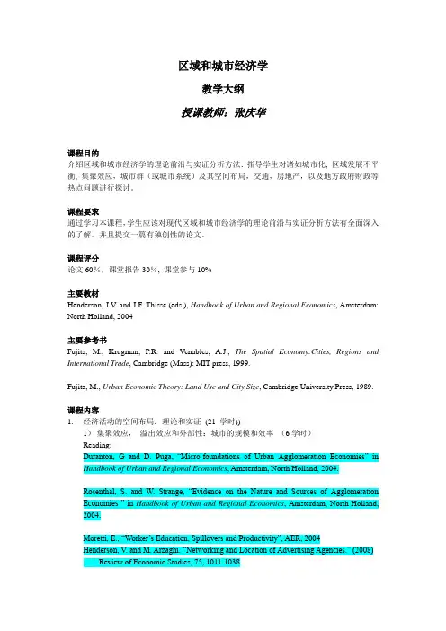
区域和城市经济学教学大纲授课教师:张庆华课程目的介绍区域和城市经济学的理论前沿与实证分析方法.指导学生对诸如城市化, 区域发展不平衡, 集聚效应,城市群(或城市系统)及其空间布局,交通,房地产,以及地方政府财政等热点问题进行探讨。
课程要求通过学习本课程,学生应该对现代区域和城市经济学的理论前沿与实证分析方法有全面深入的了解。
并且提交一篇有独创性的论文。
课程评分论文60%,课堂报告30%, 课堂参与10%主要教材Henderson, J.V. and J.F. Thisse (eds.), Handbook of Urban and Regional Economics, Amsterdam: North Holland, 2004主要参考书Fujita, M., Krugman, P.R. and Venables, A.J., The Spatial Economy:Cities, Regions and International Trade, Cambridge (Mass): MIT press, 1999.Fujita, M., Urban Economic Theory: Land Use and City Size, Cambridge University Press, 1989.课程内容1.经济活动的空间布局:理论和实证(21 学时))1)集聚效应,溢出效应和外部性:城市的规模和效率(6学时)Reading:Duranton, G and D. Puga, “Micro-foundations of Urban Agglomeration Economies” in Handbook of Urban and Regional Economics, Amsterdam, North Holland, 2004.Rosenthal, S. and W. Strange, “Evidence on the Nature and Sources of Agglomeration Economies ” in Handbook of Urban and Regional Economics, Amsterdam, North Holland, 2004.Moretti, E., “Worker’s Education, Spillovers and Productivity”, AER, 2004Henderson, V. and M. Arzaghi. “Networking and Location of Advertising Agencies.” (2008) Review of Economic Studies, 75, 1011-1038Ciccone, A. and G. Peri. “Identifying Human Capital Externalities: Theory with Applicati ons.” Review of Economic Studies (2006): 73, 381-412.Greenstone M., R. Hornbeck, and E. Moretti (2010) “Identifying Agglomeration Spillovers: Evidence from Winners and Losers of Large Plant Openings”. J. of Political EconomyBay er, P., S. Ross, and G. Topa (2008), “Place of Work and Place of Residence…”Journal of Political Economy, 116, 1150-1196Rosenthal S. and W. Strange (2008) “The Attenuation of Human Capital Spillovers,”Journal of Urban Economics, 64, 373-3892)城市群和城市系统(6学时)Reading:Henderson, J.V. and R. Becker, “Political Economy of City Sizes and Formation,” Journal of Urban Economics, 2001, (48).Black, D. and J.V. Henderson, “Urban Growth,” Journal of Political Economy, 1999, (107).Henderson, J.V., “Growth and Urbanization” in Handbook of Economic Growth, Agion and Durlauf (eds.).Duranton, “Urban Evolutions: the Still, the Slow and the Fast”, AER, 2007 (97),197-221Henderson, J.V. and A.J. V enables. (2009) “The Dynamics of City Formation.”Review of Economic Dynamics, 12, 233-254Krugman, P. (1991) "Increasing Returns and Economic Geography." Journal of Political Economy, 99, 3, 483-499.Puga, D. (1999) “The Rise and Fall of Regional Inequalities. ”European Economic Review 43, 303-334.Behrens, K., G. Duranton, and F. Robert-Nicoud (2011) “Productive cities: Sorting, Selection and Agglomeration” mimeoHelsley R. and W. Strange (2011) “Coagglomeration” Berkeley mimeoFujita, M., Krugman, P.R. and Venables, A.J., The Spatial Economy:Cities, Regions andInternational Trade, Cambridge (Mass): MIT press, 1999. Chapters 4,5,63)城市系统和经济活动空间分布的实证分析(3学时)Reading:Black, D. and J.V. Henderson, “Spatial Evolution of Population and Industry,” Papers and Proceedings of American Economic Review, May 1999.Ellison, G. and E. Glaeser, “Geographic Concentration of Industry,” Papers and Proceedings of American Economic Review, May 1999.Gabaix, X., “Zipf’s Law of Growth of Cities,” Papers and Proceedings of American Economic Review, May 1999.Au and Henderson, “Are Chinese Cities too Small?” Review of Economic Studies, 2006Duranton and Overman, “Testing for localization using micro-geographic data”, Review of Economic Studies, 20054) 搜索与匹配在城市经济学的应用(3学时)Reading:Helsley, R. and W. Strange (1990). “Matching and Agglomeration Economies in a System of Cities.” Regional Science and Urban Economics 20, 189-212.Gan and Zhang, “The Thick Market Effect on Local Unemployment Fluctuations”, Journal of Econometrics, 2006Berliant, Reed and Wang, 2000, “Knowledge Exchange, Matching, and Agglomeration.”Journal of Urban Economics 60 (2006) 69–955) 城市内部结构(3学时)Reading:Fujita, M., Urban Economic Theory: Land Use and City Size, Cambridge University Press, 1989. Chapters 2,3,4Lucas and Rossi-Hansberg, 2002, “On the Internal Structure of Cities,” Econometrica 70(4): 1445--14762.专题讨论(12学时)1)城市的工资,价值和福利:如何度量Glaeser, E., J. Scheinkman, and A. Shleifer (1995) “Economic Growth in a Cross-Section of Cities.” Journal of Monetary Economics 36, 117-143.Roback, J. 1982, “Wages, Rents and Quality of Life,” Journal of Political Economy, 1257- 1278Glaeser, E. and D. Mare (2001). “Cities and Skills.” Journal of Labor Economics.): 91, 316-342Baum-Snow, N. and R. Pavin (2011) “Understanding the City Size Wage Gap,” Review of Economic Studies, forthcomingAlbouy D. (2009) “What are Cities Worth? Land Rents, Local Productivity and the Capitalization of Amenity ValuesDesmet K. and E. Rossi_Hansberg, 2011 “Urban Accounting and Welfare”, Princeton Mimeo2)城市房地产Reading:Siqi Zheng, Matthew E.Kahn, “Land and residential property markets in a booming economy: New evidence from Beijing”, Journal o f Urban Economics 63 (2008), 743-757Saiz, A. (2010), “The geographic determinants of housing supply” Quarterly Journal of EconomicsB.Glaeser, E. and J. Gyourko (2003).”The Impact of Building Restrictions on Housing Affordability.”Economics Policy Review 9, 21-39.Haughwout, A., M. Turner, W. van der Klaauw (2011), “Land Use Regulation and Welfare”Mimeo, U. of TorontoQuigley J. and S. Raphael (2005) “Regulation and the high costs of housing” American Economic Review, 95, 323-328C.Housing Tenure Choice modelHenderson, J. V., and Y. M. Ioannides. “A Model of Housing Tenure Choice,” American Economic Review, 1983, 73 (March), 98-113.Ioannides, Y. M., and S. S. Rosenthal. “Estimating the Consumption and Investment Demands for Housing and their Effect on Housing Tenure Status,” Review of Economics and Statistics, 1994, 76 (February), 127-141.D.China’s urban housing ma rketShing-yi Wang, “Credit Constraints, Job Mobility and Entrepreneurship: evidence from a Property Reform in China,” Review of Economics and Statistics, 2012Shing-yi Wang, “State Misallocation and Housing Prices: Theory and Evidence from China,”AER 2011“The Ability to Build Up: Evidence from Matched Land Parcel and Residential Development Project Data in Chinese Cities,” with Zhi Wang, 2013“How Does Capital Gains influence Housing Tenure Choice and Housing Investment Demand: Evidence from China’s Urban Household Survey Data,” 2013, with Y ujin Cao and Hongbin Cai“Fundamentals in China’s Urban Housing Markets: Land Supply, Hukou Population, and Housing Price Appreciation,” with Zhi Wang, 2013,revision requested by Journal of Housing EconomicsNathaniel Baum‐Snow, Loren Brandt, J. Vernon Henderson, Matthew A. Turner and Qinghua Zhang (2012), Roads, Railroads and Decentralization of Chinese Cities。
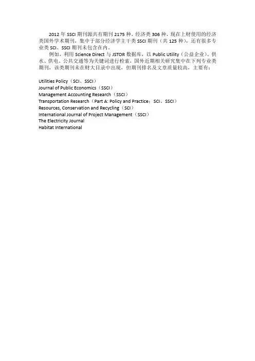
2012年SSCI期刊源共有期刊2175种,经济类306种,现在上财使用的经济类国外学术期刊,集中于部分经济学主干类SSCI期刊(共125种),还有很多专业类SCI、SSCI期刊未包含在内。
例如,利用Science Direct与JSTOR数据库,以Public Utility(公益企业)、供水、供电、公共交通等为关键词进行检索,国外近期相关研究集中在下列专业类期刊,该类期刊未在财大目录中出现,但期刊排名及文章质量较高,主要有:Utilities Policy(SCI、SSCI)Journal of Public Economics(SSCI)Management Accounting Research(SSCI)Transportation Research(Part A: Policy and Practice;SCI、SSCI)Resources, Conservation and Recycling(SCI)International Journal of Project Management(SSCI)The Electricity JournalHabitat International上财常任轨期刊(部分属于SSCI期刊源)Top Tier(顶级):EconometricaAmerican Economic ReviewJournal of Political EconomyQuarterly Journal of EconomicsReview of Economic StudiesFirst Tier(第一类):Economic JournalGames and Economic BehaviorInternational Economic ReviewJournal of EconometricsJournal of Economic TheoryJournal of FinanceJournal of International EconomicsJournal of Labor EconomicsJournal of Monetary EconomicsJournal of Public EconomicsJournal of the European Economic AssociationRand Journal of EconomicsReview of Economics and StatisticsTheoretical EconomicsSecond Tier(第二类):AEJ:Applied EconomicsAEJ:Economic PolicyAEJ:MacroeconomicsAEJ:MicroeconomicsAmerican Journal of Agricultural EconomicsAEA Papers and ProceedingsBrookings Papers on Economic ActivityCanadian Journal of EconomicsEconometric TheoryEconomic TheoryEuropean Economic ReviewExperimental EconomicsJournal of Applied EconometricsJournal of Business & Economic StatisticsJournal of Comparative EconomicsJournal of Development EconomicsJournal of Economic Behavior & OrganizationJournal of Economic Dynamics & ControlJournal of Economic EducationJournal of Economic GrowthJournal of Economic HistoryJournal of Economic LiteratureJournal of Economic PerspectivesJournal of Economics & Management Strategy Journal of Environmental Economics and Management Journal of Financial EconomicsJournal of Health EconomicsJournal of Human ResourcesJournal of Industrial EconomicsJournal of Law & EconomicsJournal of Mathematical EconomicsJournal of Money, Credit and BankingJournal of Population EconomicsJournal of Real Estate Finance and Economics Journal of Regulatory EconomicsJournal of Risk and UncertaintyJournal of Urban EconomicsMacroeconomic DynamicsReview of Economic DynamicsReview of Financial StudiesSocial Choice and WelfareThird Tier(第三类):Applied EconomicsCambridge Journal of EconomicsChina Economic ReviewContemporary Economic PolicyEconometrics JournalEconometric ReviewsEconomics and PhilosophyEconomic InquiryEconomicaEconomic Development and Cultural Change Economic History ReviewEconomic PolicyEconomic RecordEconomics LettersEconomic ModellingEconomics of Education ReviewEconomics of TransitionEmpirical EconomicsEnergy JournalEnvironmental and Resource EconomicsEurope-Asia StudiesExplorations in Economic HistoryFrontiers of Economics in ChinaHealth EconomicsIndustrial & Labor Relations ReviewIndustrial RelationsInternational Journal of Game TheoryInternational Journal of Industrial Organization International Monetary Fund Staff PapersInternational Tax and Public FinanceJournal of Accounting and EconomicsJournal of Agricultural EconomicsJournal of Banking & FinanceJournal of EconomicsJournal of Financial and Quantitative AnalysisJournal of Institutional and Theoretical EconomicsJournal of Law Economics & OrganizationJournal of MacroeconomicsJournal of Productivity AnalysisJournal of Regional ScienceJournal of Transport Economics and PolicyLabour EconomicsLand EconomicsMathematical Social SciencesNational Tax JournalRegional Science and Urban EconomicsOxford Bulletin of Economics and StatisticsOxford Economics PapersOxford Review of Economic PolicyPublic ChoiceResource and Energy EconomicsReview of Economic DesignReview of Income and WealthReview of Industrial OrganizationReview of International EconomicsScandinavian Journal of EconomicsScottish Journal of Political EconomySouthern Economic JournalThe B.E. Journal of Economic Analysis & PolicyThe B.E. Journal of MacroeconomicsThe B.E. Journal of Theoretical Economics (Contributions tier) Theory and DecisionWorld Bank Economic ReviewWorld DevelopmentWorld Economy注:①标红为财政类、政策类期刊;②该目录未涵盖所有经济类、管理类SSCI期刊;③部分经济类、管理类SCI期刊不在SSCI期刊源中。
journal of urban economics 发表经验
在《Journal of Urban Economics》这样的顶级期刊上发表论文需要经过以下几
个步骤:
1.准备充分:在投稿之前,需要充分准备论文,包括选择合适的主题、进行深入研究、
撰写论文等。
同时,还需要了解期刊的投稿要求和审稿流程,以便更好地准备投稿。
2.仔细阅读期刊要求:在投稿之前,需要仔细阅读期刊的投稿要求和审稿流程,确保
自己的论文符合期刊的要求和审稿流程。
这有助于提高论文的录用率。
3.寻找合适的导师:在投稿之前,可以寻找本领域的专家或教授进行指导,提高论文
的质量和水平。
4.投稿:按照期刊的要求准备好论文,提交给期刊编辑部。
5.等待审稿:论文会经过同行评审,由专业领域的专家对论文进行评审。
6.根据审稿意见修改:如果论文被接受,需要根据审稿意见进行修改和完善。
7.再次投稿并等待再次审稿:将修改后的论文再次提交给期刊编辑部,等待再次审稿。
8.最终录用:如果论文最终被接受,就可以在期刊上发表了。
需要注意的是,《Journal of Urban Economics》是国际知名的学术期刊,发表
论文的竞争非常激烈。
因此,要想在这样的期刊上发表论文,需要具备较高的研究水平和实力,同时还需要付出大量的努力和时间。
economist 经济学家socialist economy 社会主义经济capitalist economy 资本主义经济collective economy 集体经济planned economy 计划经济controlled economy 管制经济rural economics 农村经济liberal economy 经济mixed economy 混合经济political economy 政治经济学protectionism 保护主义autarchy 闭关自守primary sector 初级成分private sector 私营成分,私营部门public sector 公共部门,公共成分economic channels 经济渠道economic balance 经济平衡economic fluctuation 经济波动economic depression 经济衰退economic stability 经济稳定economic policy 经济政策economic recovery 经济复原understanding 约定concentration 集中holding company 控股公司trust 托拉斯cartel 卡特尔rate of growth 增长economic trend 经济趋势economic situation 经济形势infrastructure 基本建设standard of living 生活标准,生活水平purchasing power, buying power 购买力scarcity 短缺stagnation 停滞,萧条,不景气underdevelopment 不发达underdeveloped 不发达的developing 发展中initial capital 创办资本frozen capital 冻结资金frozen assets 冻结资产fixed assets 固定资产real estate 不动产,房地产circulating capital, working capital 流动资本available capital 可用资产capital goods 资本货物reserve 准备金,储备金calling up of capital 催缴资本allocation of funds 资金分配contribution of funds 资金捐献working capital fund 周转基金revolving fund 循环基金,周转性基金contingency fund 意外开支,准备金reserve fund 准备金buffer fund 缓冲基金,平准基金sinking fund 偿债基金investment 投资,资产investor 投资人self-financing 自筹经费,经费自给bank 银行current account 经常帐户(美作:checking account)current-account holder 支票帐户(美作:checking-account holder)cheque 支票(美作:check)bearer cheque, cheque payable to bearer 无记名支票,来人支票crossed cheque 划线支票traveller's cheque 旅行支票chequebook 支票簿,支票本(美作:checkbook) endorsement 背书transfer 转让,转帐,过户money 货币issue 发行ready money 现钱cash 现金ready money business, no credit given 现金交易,概不赊欠change 零钱banknote, note 钞票,纸币(美作:bill)to pay (in) cash 付现金domestic currency, local currency] 本国货币convertibility 可兑换性convertible currencies 可兑换货币exchange rate 汇率,兑换率foreign exchange 外汇floating exchange rate 浮动汇率free exchange rates 汇兑市场foreign exchange certificate 外汇兑换券hard currency 硬通货speculation 投机saving 储装,存款depreciation 减价,贬值devaluation (货币)贬值revaluation 重估价runaway inflation 无法控制的通货膨胀deflation 通货紧缩capital flight 资本外逃securities business 证券市场stock exchange 贡市场stock exchange corporation 证券交易所stock exchange 证券交易所,贡交易所quotation 报价,牌价share 股份,贡shareholder, stockholder 贡持有人,股东dividend 股息,红利cash dividend 现金配股stock investment 贡投资investment trust 投资信托stock-jobber 贡经纪人stock company, stock brokerage firm 证券公司securities 有价证券share, common stock 普通股preference stock 优先股income gain 股利收入issue 发行贡par value 股面价格, 票面价格bull 买手, 多头bear 卖手, 空头assigned 过户opening price 开盘closing price 收盘hard times 低潮business recession 景气衰退doldrums 景气停滞dull 盘整ease 松弛raising limit 涨停板break 暴跌bond, debenture 债券Wall Street 华尔街short term loan 短期贷款long term loan 长期贷款medium term loan 中期贷款lender 债权人creditor 债权人debtor 债务人,借方borrower 借方,借款人borrowing 借款interest 利息rate of interest 利率discount 贴现,折扣rediscount 再贴现annuity 年金maturity 到期日,偿还日amortization 摊销,摊还,分期偿付redemption 偿还insurance 保险mortgage 抵押allotment 拨款short term credit 短期信贷consolidated debt 合并债务funded debt 固定债务,长期债务floating debt 流动债务drawing 提款,提存aid 援助allowance, grant, subsidy 补贴,补助金,津贴short term loan 短期贷款long term loan 长期贷款medium term loan 中期贷款lender 债权人creditor 债权人debtor 债务人,借方borrower 借方,借款人borrowing 借款interest 利息rate of interest 利率discount 贴现,折扣rediscount 再贴现annuity 年金maturity 到期日,偿还日amortization 摊销,摊还,分期偿付redemption 偿还insurance 保险mortgage 抵押allotment 拨款short term credit 短期信贷consolidated debt 合并债务funded debt 固定债务,长期债务floating debt 流动债务drawing 提款,提存aid 援助allowance, grant, subsidy 补贴,补助金,津贴cost 成本,费用expenditure, outgoings 开支,支出fixed costs 固定成本overhead costs 营业间接成本overheads 杂项开支,间接成本operating costs 生产费用,营业成本operating expenses 营业费用running expenses 日常费用,经营费用miscellaneous costs 杂项费用overhead expenses 间接费用,管理费用upkeep costs, maintenance costs 维修费用,养护费用transport costs 运输费用social charges 社会负担费用contingent expenses, contingencies 或有费用apportionment of expenses 分摊费用income 收入,收益earnings 利润,收益gross income, gross earnings 总收入,总收益gross profit, gross benefit 毛利,总利润,利益毛额net income 纯收益,净收入,收益净额average income 平均收入national income 国收入profitability, profit earning capacity 利润率,赢利率yield 产量收益,收益率increase in value, appreciation 增值,升值duty 税taxation system 税制taxation 征税,纳税fiscal charges 财务税收progressive taxation 累进税制graduated tax 累进税value added tax 增值税income tax 所得税land tax 地租,地价税excise tax 特许权税basis of assessment 估税标准taxable income 须纳税的收入fiscality 检查tax-free 免税的tax exemption 免税taxpayer 纳税人tax collector 收税员China Council for the Promotion of International Trade, C.C.P.I.T. 中国国际贸易促进委员会National Council for US-China Trade 美中贸易全国理事会Japan-China Economic Association 日中经济协会Association for the Promotion of International Trade,Japan 日本国际贸易促进会British Council for the Promotion of International Trade 英国国际贸易促进委员会International Chamber of Commerce 国际商会International Union of Marine Insurance 国际海洋运输保险协会International Alumina Association 国际铝矾土协会Universal Postal Union, UPU 万国邮政联盟Customs Co-operation Council, CCC 关税合作理事会United Nations Trade and Development Board联合国贸易与发展理事会Organization for Economic cooperation and Development, DECD 经济合作与开发组织European Economic Community, EEC, European Common Market 欧洲经济共同体European Free Trade Association, EFTA 欧洲贸易联盟European Free Trade Area, EFTA 欧洲贸易区Council for Mutual Economic Aid, CMEA 经济互助委员会Eurogroup 欧洲集团Group of Ten 十国集团Committee of Twenty(Paris Club) 二十国委员会Coordinating Committee, COCOM 巴黎统筹委员会Caribbean Common Market, CCM, Caribbean Free-Trade Association, CARIFTA 加勒比共同市场(加勒比贸易同盟)Andeans Common Market, ACM, Andeans Treaty Organization, ATO 安第斯共同市场Latin American Free Trade Association, LAFTA 拉丁美洲贸易联盟Central American Common Market, CACM 中美洲共同市场African and Malagasy Common Organization, OCAM 非洲与马尔加什共同组织East African Common Market, EACM 东非共同市场Central African Customs and Economic Union, CEUCA 中非关税经济同盟West African Economic Community, WAEC 西非经济共同体Organization of the Petroleum Exporting Countries, OPEC 石油输出国组织Organization of Arab Petroleum Exporting Countries, OAPEC 阿拉伯石油输出国组织Commonwealth Preference Area 英联邦特惠区Centre National du Commerce Exterieur, National Center of External Trade 法国对外贸易中心People's Bank of China 中国人银行Bank of China 中国银行International Bank for Reconstruction and development, IBRD 国际复兴开发银行World Bank 世界银行International Development association, IDA 国际开发协会International Monetary Found Agreement 国际货币基金协定International Monetary Found, IMF 国际货币基金组织European Economic and Monetary Union 欧洲经济与货币同盟European Monetary Cooperation Fund 欧洲货币合作基金Bank for International Settlements, BIS 国际结算银行African Development Bank, AFDB 非洲开发银行Export-Import Bank of Washington 美国进出口银行National city Bank of New York 花旗银行American Oriental Banking Corporation 美丰银行American Express Co. Inc. 美国万国宝通银行The Chase Bank 大通银行Inter-American Development Bank, IDB 泛美开发银行European Investment Bank, EIB 欧洲投资银行Midland Bank,Ltd. 米兰银行United Bank of Switzerland 瑞士联合银行Dresden Bank A.G. 德累斯敦银行Bank of Tokyo,Ltd. 东京银行Hongkong and Shanghai Corporation 香港汇丰银行International Finance Corporation, IFC 国际金融公司La Communaute Financieve Africane 非洲金融共同体Economic and Social Council, ECOSOC 联合国经济及社会理事会United Nations Development Program, NUDP 联合国开发计划署United Nations Capital Development Fund, UNCDF 联合国资本开发基金United Nations Industrial Development Organization, UNIDO 联合国工业发展组织United Nations Conference on Trade and Development, UNCTAD 联合国贸易与发展会议Food and Agricultural Organization, FAO 粮食与农业组织, 粮农组织Economic Commission for Europe, ECE 欧洲经济委员会Economic Commission for Latin America, ECLA 拉丁美洲经济委员会Economic Commission for Asia and Far East, ECAFE 亚洲及远东经济委员会Economic Commission for Western Asia, ECWA 西亚经济委员会Economic Commission for Africa, ECA 非洲经济委员会Overseas Chinese Investment Company 华侨投资公司New York Stock Exchange, NYSE 纽约证券交易所London Stock Market 伦敦贡市场Baltic Mercantile and Shipping Exchange 波罗的海商业和航运交易所instruction, education 教育culture 文化primary education 初等教育secondary education 中等教育higher education 高等教育the three R's 读、写、算school year 学年term, trimester 学季semester 学期school day 教学日school holidays 假期curriculum 课程subject 学科discipline 纪律timetable 课程表class, lesson 课homework 家庭作业exercise 练习dictation 听写spelling mistake 拼写错误(short) course 短训班seminar 研讨班playtime, break 课间,休息to play truant, to play hooky 逃学,旷课course (of study) 学业student body 学生(总称)classmate, schoolmate 同学pupil 小学生student 大学生schoolboy 男生schoolgirl 女生auditor 旁听生swot, grind 用的学生old boy 老生grant, scholarship, fellowship 奖学金holder of a grant, scholar, fellow 奖学金获得者school uniform 校服teaching staff 教育工作者(总称)teachers 教师(总称)primary school teacher 小学老师teacher lecturer 大学老师professor 教授schooling 教授,授课assistant 助教headmaster 校长(女性为:headmistress) deputy headmaster, deputy head 副校长rector 校长dean 教务长laboratory assistant, lab assistant 实验员beadle, porter 门房,学校工友games master, gym teacher, gym instructor 体育教师private tutor 私人教师,家庭教师pedagogue 文学教师(蔑称)of school age 教龄beginning of term 开学matriculation 注册to enroll, to enroll 予以注册to take lessons (学生)上课to teach (老师)上课to study 学习to learn by heart 记住,掌握to revise, to go over 复习test 考试to test 考试to take an examination, to sit an examination, to do an examination 参加考试convocation notice 考试通知examiner 考试者board of examiners 考试团examination oral, written examination 口试,笔试question 问题question paper 试卷crib 夹带(美作:trot)to pass an examination (或exam), 通过考试pass, passing grade 升级prizegiving 分配奖品to fall an examination 未通过考试failure 未考好to repeat a year 留级degree 学位graduate 毕业生to graduate 毕业project, thesis 毕业论文General Certificate of Education 中学毕业证书(美作:high school diploma)holder of the General Certificate of Education 中学毕业生(美作:holder of a high school diploma) doctorate 博士学位doctor 博士competitive examination 答辩考试Chinese 语文English 英语Japanese 日语mathematics 数学science 理科gymnastics 体育history 历史algebra 代数geometry 几何geography 地理biology 生物chemistry 化学physics 物理physical geography 地球物理literature 文学sociology 社会学psycology 心理学philosophy 哲学engineering 工程学mechanical engineering 机械工程学electronic engineering 电子工程学medicine 医学social science 社会科学agriculture 农学astronomy 天文学economics 经济学politics 政治学commercial science 商学biochemistry 生物化学anthropology 人类学linguistics 语言学accounting 会计学law, jurisprdence 法学banking 银行学metallurgy 冶金学finance 财政学mass-communication 大众传播学journalism 新闻学atomic energy 原子能学civil engineering 土木工程architecture 建筑学chemical, engineering 化学工程accounting and statisics 会计统计business administration 工商管理library 图书馆学diplomacy 外交foreign language 外文botany 植物major 主修minor 辅修school 学校kindergarten 幼儿园infant school 幼儿学校primary school, junior school 小学secondary school 中学high school, secondary school 专科学校business school 商业学校technical school 工业学校technical college 专科学校(university) campus 大学university 大学boarding school 供膳宿的学校day school 日校,无宿舍学校,走读学校day student who has lunch at school 提供午餐的走读学生academy 专科学院faculty 系hall of residence 学校公寓classroom 教室lecture theatre 阅览室(美作:lecture theater) amphitheatre 阶梯教室(美作:amphitheater) staff room 教研室headmaster's study, headmaster's office 校长办公室(assembly) hall 礼堂library 图书馆playground 操场desk 课桌blackboard 黑板(a piece of) chalk 粉笔slate pencil 石板笔wall map 挂图skeleton map 廓图,示意图globe 地球仪text book 课本dictionary 词典encyclopedia 百科全书atlas地图集satchel 书包exercise book 练习本rough not book 草稿本(美作:scribbling pad) blotting paper 吸墨纸tracing paper 描图纸squared paper, graph paper 坐标纸(fountain) pen 自来水笔biro, ballpoint (pen) 圆珠笔pencil 铅笔propelling pencil 自动铅笔pencil sharpener 铅笔刀,转笔刀ink 墨水inkwell 墨水池rubber, eraser 橡皮ruler, rule 尺slide rule 计算尺set square 三角板protractor 量角器compass, pair of compasses 圆规Ministry of Labour 劳工部(美作epartment of Labor)labour market 劳工市场, 劳务市场Labour exchange, Employment exchange 职业介绍所(美作:Employment Bureau)labour management 职业介绍经纪人full employment 整日制工作to be paid by the hour 按小时付酬seasonal work 季节工作piecework work 计件工作timework work 计时工作teamwork work 联合工作shift work 换班工作assembly line work 组装线工作(美作:serial production)workshop 车间handicrafts, crafts 手艺, 技艺trade, craft 行当profession, occupation 职务employment, job 工作situation, post 位置job 一件工作vacancy 空缺, 空额work permit 工作许可证to apply for a job 求职, 找工作application(for a job) 求职to engage, to employ 雇用work contract 劳务合同industrial accident 劳动事故occupational disease 职业病vocational guidance 职业指导vocational training 职业训练retraining, reorientation, rehabilitation 再训练, 再培训holidays, holiday, vacation 假期labour costs, labour input 劳力成本fluctuation of labour 劳力波动(美作 f labor) worker 工作者permanent worker 长期工, 固定工personnel, staff 人员employee 职员clerk, office worker 办公室人员salary earner 雇佣工人workman 工人organized labour 参加工会的工人skilled worker 技术工人unskilled worker 非技术工人specialized worker 熟练工人farm worker 农场工人labourer worker 农业工人day labourer 日工seasonal worker 季节工collaborator 合作者foreman 工头trainee, apprentice 学徒工apprenticeship 学徒artisan, craftsman 工匠specialist 专家night shift 夜班shortage of labour, shortage of manpower 缺乏劳力working class 工人阶级proletarian 无产者proletariat 无产阶级trade union 工会(美作:labor union)trade unionist 工团主义者trade unionism 工团主义guild 行会,同会,公会association, society, union 协会emigration 移,移居employer 雇主,老板shop steward (工厂的)工会代表(美作:union delegate) delegate 代表representative 代表works council 劳资联合委员会labour law 劳工法working day, workday 工作日full-time employment, full-time job, full-time work 全天工作part-time employment, part-time job, part-time work 半日工作working hours 工作时间overtime 业余时间remuneration 报酬pay, wage, salary 工资wage index 工资指数minimum wage 最低工资basic wage 基础工资gross wages 全部收入net, real wages 实际收入hourly wages, wage rate per hour 计时工资monthly wages 月工资weekly wages 周工资piecework wage 计件工资maximum wage 最高工资(美作:wage ceiling) sliding scale 按物价计酬法payment in kind 用实物付酬daily wages 日工资premium, bonus, extra pay 奖励payday 发工资日, 付薪日pay slip 工资单payroll 薪水册unemployment benefit 失业救济old-age pension 退休金,养老金collective agreement 工会代表工人与资方代表达成的协议retirement 退休claims 要求strike 罢工striker 罢工者go-slow 怠工(美作:slow-down)lockout 停工(业主为抵制工人的要求而停工) staggered strike 阶段性罢工strike picket 罢工纠察队员strike pay 罢工津贴(由工会给的) strikebreaker, blackleg 破坏罢工者down tools, sit-down strike 静坐demonstration, manifestation 示威sanction 制裁unemployment 失业seasonal unemployment 季节性失业underemployment 不充分就业unemployed man 失业者(个人)the unemployed 失业者(集体)to discharge, to dismiss 辞退,开除,解雇dismissal 开除,解雇to terminate a contract 结束合同,结束契约negotiation 谈判collective bargaining 劳资双方就工资等问题谈判receptionist 接待员typist 打字员key puncher 电脑操作员stenographer 速记员telephone operator 电话接线员programmer 电脑程序员system analyst 系统分析员shorthand typist 速记打字员office girl 女记事员public servants 公务员national public servant 国家公务员local public service employee 地方公务员nation railroad man 国营铁路职员tracer 绘图员illustrator 汇稿员saleswoman 女店员pilot 驾驶员simultaneous 同时译员publisher 出版人员graphic designer 美术设计员delivery boy 送报员secretary 秘书policeman 警察journalist 记者editor 编辑interpreter 通译者director 导演talent 星探actor 男演员actress 女演员photographer 摄影师scholar 学者translator 翻译家novelist 小说家playwright 剧作家linguist 语言学家botanist 植物学家economist 经济学家chemist 化学家scientist 科学家philosopher 哲学家politician 政治学家physicist 物理学家astropologist 人类学家archaeologist 考古学家geologist 地质学家expert on folklore 俗学家mathematician 数学家biologist 生物学家zoologist 动物学家statistician 统计学家physiologist 生理学家futurologist 未来学家artists 艺术家painter 画家musician 音乐家composer 作曲家singer 歌唱家designer 设计家sculptor 雕刻家designer 服装设计师fashion coordinator 时装调配师dressmaker 女装裁剪师cutter 裁剪师sewer 裁缝师tailor 西装师傅beautician 美容师model 模特ballerina 芭蕾舞星detective 刑警chief of police 警察局长taxi driver 出租车司机clerk 店员mailman 邮差newspaper boy 报童bootblack 擦鞋童poet 诗人copywriter 撰稿人producer 制片人newscaster 新闻评论人milkman 送奶人merchant 商人florist 卖花人baker 面包师greengrocer 菜贩fish-monger 鱼贩butcher 肉贩shoe-maker 鞋匠saleswoman 女店员stewardess 空中小姐conductor 车掌station agent 站长porter 行李夫car mechanic 汽车修理师architect 建筑师civil planner 城市设计师civil engineer 土木技师druggist, chemist, pharmacist 药剂师guide 导游oil supplier 加油工(public) health nurse 保健护士dentist 牙科医生supervisor 监工forman 工头doctor 医生nurse 护士宏观经济的macroeconomic 通货膨胀inflation破产insolvency有偿还债务能力的solvent合同contract汇率exchange rate紧缩信贷tighten credit creation私营部门private sector财政管理机构fiscal authorities宽松的财政政策slack fiscal policy税法tax bill财政public finance财政部the Ministry of Finance平衡预算balanced budget继承税inheritance tax货币主义者monetariest增值税VAT (value added tax)收入revenue总需求aggregate demand货币化monetization赤字deficit经济不景气recessiona period when the economy of a country is not successful, business conditions are bad, industrialproduction and trade are at a low level and there is a lot of unemployment经济好转turnabout复苏recovery成本推进型cost push货币供应money supply生产率productivity劳动力labor force实际工资real wages成本推进式通货膨胀cost-push inflation需求拉动式通货膨胀demand-pull inflation双位数通货膨胀double- digit inflation极度通货膨胀hyperinflation长期通货膨胀chronic inflation治理通货膨胀to fight inflation最终目标ultimate goal坏的影响adverse effect担保ensure贴现discount萧条的sluggish认购subscribe to支票帐户checking account货币控制工具instruments of monetry control 借据IOUs(I owe you)本票promissory notes货币总监controller of the currency拖收系统collection system支票清算或结算check clearing资金划拨transfer of funds可以相信的证明credentials改革fashion被缠住entangled货币联盟Monetary Union再购协议repo精明的讨价还价交易horse-trading欧元euro公共债务membership criteria汇率机制REM储备货币reserve currency劳动密集型labor-intensive贡交易所bourse竞争领先frontrun牛市bull market非凡的牛市 a raging bull规模经济scale economcies 买方出价与卖方要价之间的差价bid-ask spreads 期货(贡)futures经济商行brokerage firm回报率rate of return贡equities违约default现金外流cash drains经济人佣金brokerage fee存款单CD(certificate of deposit营业额turnover资本市场capital market布雷顿森林体系The Bretton Woods System经常帐户current account套利者arbitrager远期汇率forward exchange rate即期汇率spot rate实际利率real interest rates货币政策工具tools of monetary policy银行倒闭bank failures跨国公司MNC ( Multi-National Corporation)商业银行commercial bank商业票据comercial paper利润profit本票,期票promissory notes监督to monitor佣金(经济人)commission brokers套期保值hedge有价证券平衡理论portfolio balance theory外汇储备foreign exchange reserves固定汇率fixed exchange rate浮动汇率floating/flexible exchange rate货币选择权(期货)currency option套利arbitrage合约价exercise price远期升水forward premium多头买升buying long空头卖跌selling short按市价订购贡market order贡经纪人stockbroker国际货币基金the IMF七国集团the G-7监督surveillance同业拆借市场interbank market可兑换性convertibility软通货soft currency限制restriction交易transaction充分需求adequate demand短期外债short term external debt汇率机制exchange rate regime直接标价direct quotes资本流动性mobility of capital赤字deficit本国货币domestic currency外汇交易市场foreign exchange market 国际储备international reserve利率interest rate资产assets国际收支balance of payments贸易差额balance of trade繁荣boom债券bond资本captial资本支出captial expenditures商品commodities商品交易所commodity exchange期货合同commodity futures contract普通贡common stock联合大企业conglomerate货币贬值currency devaluation通货紧缩deflation折旧depreciation贴现率discount rate 归个人支配的收入disposable personal income 从业人员employed person汇率exchange rate财政年度fiscal year企业free enterprise国生产总值gross antional product库存inventory劳动力人数labor force债务liabilities市场经济market economy合并merger货币收入money income跨国公司Multinational Corproation个人收入personal income优先贡preferred stock价格收益比率price-earning ratio优惠贷款利率prime rate利润profit回报return on investment使货币升值revaluation薪水salary季节性调整seasonal adjustment关税tariff失业人员unemployed person效用utility价值value工资wages工资价格螺旋上升wage-price spiral收益yield补偿贸易compensatory trade, compensated deal储蓄银行savings banks欧洲联盟the European Union单一的实体 a single entity抵押贷款mortgage lending业主产权owner''''s equity普通股common stock无形资产intangible assets收益表income statement营业开支operating expenses行政开支administrative expenses现金收支一览表statement of cash flow贸易中的存货inventory收益proceeds投资银行investment bank机构投资者institutional investor垄断兼并委员会MMC招标发行issue by tender定向发行introduction代销offer for sale直销placing公开发行public issue信贷额度credit line国际债券international bonds欧洲货币Eurocurrency利差interest margin以所借的钱作抵押所获之贷款leveraged loan权利股发行rights issues净收入比例结合net income gearing外贸中常见英文缩略词1 C&F(cost&freight)成本加运费价2 T/T(telegraphic transfer)电汇3 D/P(document against payment)付款交单4 D/A (document against acceptance)承兑交单5 C.O (certificate of origin)一般原产地证6 G.S.P.(generalized system of preferences)普惠制7 CTN/CTNS(carton/cartons)纸箱8 PCE/PCS(piece/pieces)只、个、支等9 DL/DLS(dollar/dollars)美元10 DOZ/DZ(dozen)一打11 PKG(package)一包,一捆,一扎,一件等12 WT(weight)重量13 G.W.(gross weight)毛重14 N.W.(net weight)净重15 C/D (customs declaration)报关单16 EA(each)每个,各17 W (with)具有18 w/o(without)没有19 FAC(facsimile)传真20 IMP(import)进口21 EXP(export)出口22 MAX (maximum)最大的、最大限度的23 MIN (minimum)最小的,最低限度24 M 或MED (medium)中等,中级的25 M/V(merchant vessel)商船26 S.S(steamship)船运27 MT或M/T(metric ton)公吨28 DOC (document)文件、单据29 INT(international)国际的30 P/L (packing list)装箱单、明细表31 INV (invoice)发票32 PCT (percent)百分比33 REF (reference)参考、查价34 EMS (express mail special)特快传递35 STL.(style)式样、款式、类型36 T或LTX或TX(telex)电传37 RMB(renminbi)人币38 S/M (shipping marks)装船标记39 PR或PRC(price) 价格40 PUR (purchase)购买、购货41 S/C(sales contract)销售确认书42 L/C (letter of credit)信用证43 B/L (bill of lading)提单44 FOB (free on board)离岸价45 CIF (cost,insurance&freight)成本、保险加运费价补充:CR=credit贷方,债主DR=debt借贷方(注意:国外常说的debt card,就是银行卡,credit card就是信誉卡。
常见的建筑术语的英文翻译集之一以下是一些常见的建筑术语的英文翻译集合之一:1. 建筑设计- Architectural Design2. 建筑结构- Building Structure3. 建筑材料- Building Materials4. 建筑施工- Building Construction5. 建筑成本- Construction Cost6. 建筑风格- Architectural Style7. 建筑师- Architect8. 建筑规划- Building Planning9. 建筑模型- Architectural Model10. 建筑面积- Building Area11. 建筑高度- Building Height12. 建筑容积率- Plot Ratio13. 建筑法规- Building Codes and Regulations14. 建筑节能- Energy Efficiency in Buildings15. 建筑智能化- Intelligent Buildings16. 绿色建筑- Green Buildings17. 可持续建筑- Sustainable Buildings18. 建筑声学- Architectural Acoustics19. 建筑光学- Architectural Optics20. 室内设计- Interior Design21. 景观设计- Landscape Design22. 结构设计- Structural Design23. 给排水设计- Water Supply and Drainage Design24. 暖通空调设计- HVAC Design25. 电气设计- Electrical Design26. 消防设计- Fire Protection Design27. 智能化系统设计- Intelligent System Design28. 施工组织设计- Construction Organization Design29. 施工图设计- Construction Drawing Design30. 装饰装修设计- Decoration and Finishing Design31. 建筑声学设计- Architectural Acoustics Design32. 建筑光学设计- Architectural Optics Design33. 建筑热工设计- Architectural Thermal Design34. 建筑美学设计- Architectural Aesthetic Design35. 建筑环境设计- Architectural Environment Design36. 建筑风水学- Feng Shui37. 建筑日照分析- Solar Analysis for Buildings38. 建筑通风分析- Ventilation Analysis for Buildings39. 建筑声环境分析- Acoustic Environment Analysis for Buildings40. 建筑光环境分析- Daylighting Environment Analysis for Buildings41. 建筑热环境分析- Thermal Environment Analysis for Buildings42. 建筑面积计算- Building Area Calculation43. 建筑楼层高度- Storey Height44. 建筑消防设计- Fire Protection Design for Buildings45. 建筑结构安全评估- Structural Safety Evaluation for Buildings46. 建筑抗震设计- Seismic Design for Buildings47. 建筑防洪设计- Flood-resistant Design for Buildings48. 建筑工程招标- Building Engineering Tendering49. 建筑工程施工许可- Construction Permission for Building Projects50. 建筑工程造价咨询- Engineering Cost Consulting for Building Projects51. 建筑工程监理- Project Supervision for Building Projects52. 建筑工程验收- Acceptance of Building Projects53. 建筑工程质量检测- Quality Detection of Building Projects54. 建筑工程质量评估- Quality Evaluation of Building Projects55. 建筑工程质量保修- Quality Guarantee of Building Projects56. 建筑工程档案- Construction Project Archives57. 建筑工程安全- Construction Safety58. 建筑工程管理- Construction Project Management59. 建筑工程合同- Construction Contract60. 建筑工程保险- Construction Insurance61. 建筑工程材料- Construction Materials62. 建筑工程机械- Construction Machinery63. 建筑工程劳务- Construction Labor64. 建筑工程施工组织设计- Construction Organization Design for Building Projects65. 建筑工程施工图设计- Construction Drawing Design for Building Projects66. 建筑工程施工进度计划- Construction Progress Plan for Building Projects67. 建筑工程施工质量控制- Construction Quality Control for Building Projects68. 建筑工程施工安全管理- Construction Safety Management for Building Projects69. 建筑工程施工现场管理- Construction Site Management for Building Projects70. 建筑工程施工成本管理- Construction Cost Management for Building Projects71. 建筑工程施工环境保护- Environmental Protection in Building Construction72. 建筑工程施工节能管理- Energy-saving Management in Building Construction73. 建筑工程施工水土保持- Soil and Water Conservation in Building Construction74. 建筑工程施工质量控制要点- Key Points of Construction Quality Control for Building Projects75. 建筑工程施工安全控制要点- Key Points of Construction Safety Control for Building Projects76. 建筑工程施工质量验收规范- Acceptance Specification for Construction Quality ofBuilding Projects77. 建筑立面设计- Façade Design78. 建筑剖面设计- Section Design79. 建筑立面分析图- Façade Analysis Diagram80. 建筑剖面分析图- Section Analysis Diagram81. 建筑结构分析图- Structural Analysis Diagram82. 建筑平面图- Floor Plan83. 建筑立面图- Façade Drawing84. 建筑剖面图- Section Drawing85. 建筑轴测图- Axonometric Drawing86. 建筑渲染图- Architectural Rendering87. 建筑模型制作- Model Making88. 建筑绘画- Architectural Drawing89. 建筑表现图- Architectural Representation90. 建筑动画- Architectural Animation91. 建筑摄影- Architectural Photography92. 建筑信息模型- Building Information Modeling (BIM)93. 建筑环境评估- Building Environmental Assessment94. 建筑节能评估- Building Energy Efficiency Assessment95. 建筑可持续性评估- Building Sustainability Assessment96. 建筑健康评估- Building Health Assessment97. 建筑设备系统设计- Building Equipment System Design98. 建筑电气系统设计- Electrical System Design for Buildings99. 建筑给排水系统设计- Water Supply and Drainage System Design for Buildings 100. 建筑暖通空调系统设计- HVAC System Design for Buildings一般建筑术语英文翻译之二101. 建筑燃气系统设计- Gas System Design for Buildings102. 建筑消防报警系统设计- Fire Alarm System Design for Buildings103. 建筑智能化系统集成设计- Intelligent System Integration Design for Buildings 104. 建筑幕墙设计- Curtain Wall Design105. 建筑石材幕墙设计- Stone Curtain Wall Design106. 建筑玻璃幕墙设计- Glass Curtain Wall Design107. 建筑绿化设计- Greening Design for Buildings108. 建筑景观设计- Landscape Design for Buildings109. 建筑室内环境设计- Indoor Environmental Design for Buildings110. 建筑声学装修设计- Acoustic Decoration Design for Buildings111. 建筑光学装修设计- Optical Decoration Design for Buildings112. 建筑材料装修设计- Decorative Materials Design for Buildings113. 建筑历史与理论- Architectural History and Theory114. 建筑美学史- History of Architectural Aesthetics115. 现代建筑设计- Modern Architectural Design116. 后现代建筑设计- Postmodern Architectural Design117. 当代建筑设计- Contemporary Architectural Design118. 解构主义建筑设计- Deconstructivist Architectural Design119. 装饰艺术建筑设计- Art Deco Architectural Design120. 功能主义建筑设计- Functionalist Architectural Design121. 结构主义建筑设计- Structuralist Architectural Design122. 新古典主义建筑设计- Neoclassical Architectural Design123. 折衷主义建筑设计- Eclectic Architectural Design124. 绿色建筑设计- Green Architectural Design125. 人文主义建筑设计- Humanist Architectural Design126. 新地域主义建筑设计- New Regionalist Architectural Design127. 参数化建筑设计- Parametric Architectural Design128. 数字建筑设计- Digital Architectural Design129. 未来主义建筑设计- Futurist Architectural Design130. 智能化建筑设计- Intelligent Building Design131. 生态建筑设计- Ecological Architectural Design132. 城市设计- Urban Design133. 景观设计- Landscape Design134. 城市规划- Urban Planning135. 城市更新- Urban Renewal136. 城市改造- Urban Transformation137. 城市意象- Urban Image138. 城市设计理论- Urban Design Theory139. 城市生态设计- Urban Ecological Design140. 城市交通设计- Urban Transportation Design141. 城市基础设施设计- Urban Infrastructure Design142. 城市天际线设计- Urban Skyline Design143. 城市夜景设计- Urban Nightscape Design144. 城市滨水区设计- Urban Waterfront Design145. 城市开放空间设计- Urban Open Space Design146. 城市街道景观设计- Urban Streetscape Design147. 城市公园设计- Urban Park Design148. 城市居住区设计- Urban Residential District Design149. 城市商业区设计- Urban Commercial District Design150. 城市文化区设计- Urban Cultural District Design151. 城市行政中心设计- Urban Governmental District Design152. 城市会展中心设计- Urban Exhibition and Convention Center Design 153. 城市体育馆设计- Urban Stadium Design154. 城市图书馆设计- Urban Library Design155. 城市博物馆设计- Urban Museum Design156. 城市大剧院设计- Urban Theater Design157. 城市机场设计- Urban Airport Design158. 城市火车站设计- Urban Train Station Design159. 城市地铁站设计- Urban Subway Station Design160. 城市公交车站设计- Urban Bus Stop Design161. 城市景观照明设计- Urban Landscape Lighting Design162. 城市标识系统设计- Urban Signage System Design163. 城市公共艺术装置设计- Public Art Installation Design164. 城市家具设计- Urban Furniture Design165. 城市花坛设计- Urban Flower Bed Design166. 城市儿童游乐设施设计- Urban Playground Design167. 城市植栽设计- Urban Planting Design168. 城市排水系统设计- Urban Drainage System Design169. 城市防洪系统设计- Urban Flood Control System Design170. 城市消防系统设计- Urban Fire Protection System Design171. 城市应急救援系统设计- Urban Emergency Rescue System Design172. 城市废弃物处理系统设计- Urban Waste Management System Design 173. 城市给水系统设计- Urban Water Supply System Design174. 城市污水处理系统设计- Urban Wastewater Treatment System Design 175. 城市雨水排放系统设计- Urban Stormwater Management System Design 176. 城市空调系统设计- Urban Air Conditioning System Design177. 城市供暖系统设计- Urban Heating System Design178. 城市燃气供应系统设计- Urban Gas Supply System Design179. 城市电力供应系统设计- Urban Electrical Power Supply System Design180. 城市智能化管理系统设计- Urban Intelligent Management System Design 181. 城市绿色建筑认证体系- Green Building Certification Systems182. 城市绿色建筑评价体系- Green Building Evaluation Systems183. 可持续城市发展理论- Sustainable Urban Development Theory 184. 生态城市理论- Eco-city Theory185. 低碳城市理论- Low-carbon City Theory186. 紧凑城市理论- Compact City Theory187. 智慧城市理论- Smart City Theory188. 韧性城市理论- Resilient City Theory189. 多规合一城市规划体系- Integrated Urban Planning System 190. 城市设计哲学- Urban Design Philosophy191. 城市设计心理学- Urban Design Psychology192. 城市设计社会学- Urban Design Sociology193. 城市设计地理学- Urban Design Geography194. 城市设计经济学- Urban Design Economics195. 城市设计生态学- Urban Design Ecology196. 城市设计符号学- Urban Design Semiotics197. 城市设计现象学- Urban Design Phenomenology198. 城市设计未来学- Urban Design Futures Studies199. 城市设计艺术史- Urban Design Art History200. 城市设计与公共政策- Urban Design and Public Policy。
营销方面的期刊Journal of Services MarketingInternational Journal of Research in MarketingJournal of Consumer MarketingJournal of marketingJournal of the Academy of Marketing ScienceHarvard business reviewJournal of Health care marketingJournal of marketing management国外经济学期刊排名TABLE I JOURNAL RANKINGS BASED ON PER ARTICLE IMPACT Econometrica(计量经济学)102.6 86.9 1.1Quarterly Journal of Economics (经济学季刊杂志)101.4 119.6 1.5 Journal of Economic Literature (经济学文献杂志)80.6 88.6 2.7 American Economic Review(美国经济评论不包括美国经济评论会议论文)77.9 92.8 1.7Journal of Political Economy(政治经济学杂志)68.6 74.8 1.0 Review of Economic Studies (经济研究评论)66.0 67.4 1.3Journal of Monetary Economics(货币经济学杂志)47.3 59.9 1.8 Journal of Economic Theory (经济学理论杂志)35.3 27.1 0.7 Games and Economic Behavior (博弈与经济行为)33.4 26.0 1.1Journal of Economics Perspectives (经济学展望杂志)31.8 34.6 0.9 上面是前10Journal of Econometrics (计量经济学杂志)21.7 15.6 1.2Rand Journal of Economics 20.6 16.4 0.8Economic Theory 18.7 16.9 1.0Journal of Labor Economics 17.8 17.5 0.8Journal of Human Resources 17.4 16.2 0.8Journal of Public Economics 16.7 16.8 1.0Review of Economics and Statistics 16.7 17.1 0.9Econometric Theory 16.5 10.1 0.7Journal of Risk and Uncertainty 16.2 17.2 0.7International Economic Review(国际经济学评论)16.0 15.3 0.9上面是前20Journal of Financial Economics 15.4 13.3 1.1Journal of Business and Ec. Statistics 15.2 12.3 0.4AER Papers and Proceedings (美国经济评论会议论文)14.0 14.9 0.4 Journal of Applied Econometrics 13.3 12.1 1.5European Economic Review 13.3 14.2 1.0International Journal of Game Theory 13.2 10.6 0.4Social Choice and Welfare 12.8 7.7 1.0J. of Environmental Ecs.and Management 12.5 9.9 0.7Economic Journal 12.2 12.6 0.8Journal of International Economics 11.7 18.2 1.5上面是前30Journal of Ec. Dynamics and Control 10.8 10.0 1.0Journal of Mathematical Economics 10.3 6.2 0.8Economic Inquiry 6.3 7.2 0.7Journal of Ec. Behavior and Organization(经济行为与组织杂志)5.3 4.9 0.9Scandinavian Journal of Economics 4.3 4.4 0.5Economics Letters 3.2 2.8 0.5Oxford Bulletin of Ecs.and Statistics 2.7 2.2 1.0国外经济学核心期刊刊名中文名称国别排名ISSNAmerican Economic Review 美国经济评论美1 0002-8282 馆藏信息The Journal of Industrial Economics 工业经济学杂志美79 0022-1821 馆藏信息The Economist 经济学家英2 0013-0613 馆藏信息The Quarterly Journal of Economics 经济学季刊美5 0033-5533 馆藏信息Journal of Economic Literature 经济文献杂志美6 0022-0515 Academy of management journal 管理学会杂志美7Harvard Business Review哈佛商业评论美9 0017-8012馆藏信息Journal of economic theory 经济理论杂志美21Brookings papers on economic activity 布鲁金斯经济活动论文集美23 Journal of Marketing 市场营销杂志美12 0022-2429The Journal of Economic Perspectives 经济展望杂志美15 0895-3309 The Review of Economic Studies 经济研究评论英16 0034-6527 Journal of Marketing Research 市场营销杂志研究美17 0022-2437 Journal of Business 商业杂志美27 0021-9398International economic review 国际经济评论美49 馆藏信息European Economic Review 欧洲经济评论荷40 0014-2921 Industrial Relations 劳资关系美52 0019-8676Business Week 商业周刊美56 0007-7135 馆藏信息Journal of Labour Economics 劳动经济学杂志美58Oxford Economic Papers 牛津经济论文集英78 0030-7653 馆藏信息Journal of Advertising Research 广告研究杂志美81 0021-8499Games and Economic Behavior 对策与经济行为美93 0899-8256 Journal of Retailing 零售杂志美99 0022-4359British Journal of Industrial Relations 英国劳资关系杂志英107 0007-1080International Journal of Industry Organization 国际产业组织杂志荷117International Journal of Game Theory 国际博弈论杂志德1190020-7276International Journal of Service Industry Management 国际服务行业管理杂志英142 0956-4233Journal of environmental economics & management 环境经济学与环境管理杂志美44Rand journal of economics 兰德经济学杂志美35 馆藏信息Journal of Regulatory Economics 管制经济学杂志美99 0922-680X 馆藏信息Journal of Law and Economics 法律与经济学杂志美Journal of Law, Economics and Organization 法律、经济学与组织杂志美馆藏信息Journal of Economics and Management Strategy) 经济学与管理策略杂志美馆藏信息Review of Industrial Organization 产业组织学评论美馆藏信息SSRN Industrial organization and Regulation Abstracts SSRN产业组织与规制文献美经管类中文核心期刊。
1American economic review2The Economist3Econometrica4Journal of political economy5Quarterly journal of economics,6the Journal of economic literature7Academy of management journal8Journal of finance9Harvard business review10Academy of management review11Journal of financial economics12Journal of marketing13Strategic management journal14Economic journal15the Journal of economic perspectives16Review of economic studies17Journal of marketing research18Review of economics&statistics19the Journal of consumer research20Journal of econometrics21Journal of economic theory22Health care financing review23Brookings papers on economic activity24Journal of monetary economics25Sloan management review26 Journal of law&economics27Journal of business28Journal of health economics29Industrial&labor relations review30Risk analysis31 Journal of human resources32Economy and society33 World development34Journal of business&economic statistics35 Rand journal of economics36Journal of public economics37Human resource management38American journal of agricultural economics39Journal of operational research society40European economic review41Review of financial studies42 Health economics43California management review44Journal of environmental economics&management 45Fortune46 World bank economic review47Journal of international economics48Journal of law,economics&organization49 International economic review50 Journal of money,credit&banking51Economic geography52 Industrial relations53Journal of product innovation management 54Journal of applied econometrics55Journal of international business studies 56Business week57Oxford bulletin of economics&statistics58Journal of labor economics59Journal of development economics60 Journal of economic history61Forbes62 Financial management63Journal of urban economics64 Marketing science65Monthly labor review66Economics letters67Economic history review68Economica69Land economics70Ecological economics71Journal of common market studies72Journal of financial&quantitative analysis73 Southern economic journal74 Economic inquiry75Economic&political weekly76Business insurance77Journal of business ethics78Oxford economics papers79 Journal of industrial economics80National tax journal81Journal of advertising research82Accounting organization and society83 Explorations in economic history84Journal of accounting research85 Public choice86Cambridge journal of economics87Economic development and cultural change 88 Work,employment and society89Business lawyer90 Journal of banking and finance91Journal of public policy&marketing92 Journal of international money&finance93 Games and economic behavior94 Journal of economic dynamics&control95Applied economics96 Development&change97International monetary fund staff papers98Journal of economic behavior&organization99Journal of retailing100Journal of development studies,the101Journal of rural studies102 Industrial marketing management103Journal of risk&uncertainty104 Journal of transport economics&policy105Journal of comparative economics5106Journal of productivity analysis107British journal of industrial relations108Journal of business research109 Econometric theory110Journal of regional science111Regional science&urban economics112 Scandinavian journal of economic113Journal of accounting&economics114 World economy,the115Long range planning116International journal of forecasting117International journal of industrial organization 118Journal of mathematical economics119 International journal of game theory120Journal of economic issues121Canadian journal of economics122Journal of business venturing123Journal of agricultural economics124Journal of risk&insurance125Journal of financial intermediation126 Journal of taxation127Futures:the magazine commodities&options128Business history129 Euromoney130Scottish journal of political economy131Weltwirtschaftliches archiv/review of worldeconomy132Journal of real estate finance&economics133Journal of portfolio management134Journal of world trade135Journal of economic education136Insurance:mathematics&economics137Auditing138Journal of world business139Journal of institutional&theoretical economics 140Economic record141History of political economy142International journal of service industrymanagement 143 Banker,the144Journal of regulatory economics145 Risk management review146OECD observer,the147Challenge148Survey of current business149Federal reserve bulletin150Transnational corporation美国经济评论 美国经济学家英国计量经济学英国政治经济学杂志美国经济学季刊美国经济文献杂志 美国6管理学会志美国7金融杂志美国8哈佛商业评论美国9管理学会评论美国10金融经济学杂志瑞士11市场营销杂志美国12战略管理杂志英国13经济学杂志英国14经济展望杂志美国15经济研究评论英国16市场营销研究杂志美国17经济学与统计学评论美国18消费者研究杂志美国19经济计量学杂志瑞士20经济理论杂志美国21卫生保健资金筹措评论美国22布鲁金斯经济活动论文集美国23货币经济学杂志荷兰24斯隆管理评论美国25法律与经济学杂志美国26商业杂志美国27卫生经济学杂志荷兰28劳资关系评论美国29风险分析美国30人力资源杂志美国31经济与社会英国32世界发展荷兰33商业与经济统计学杂志美国34兰德经济学杂志美国35公共经济学杂志瑞士36人力资源管理美国37美国农业经济学杂志美国38英国运筹学杂志英国39欧洲经济评论荷兰40金融研究评论美国41卫生经济学英国42加利福尼亚管理评论美国环境经济学与环境管理杂美国44幸福(或翻译:财富)美国45世界银行经济评论美国46国际经济学杂志荷兰47法律、经济学与组织学杂志美国48国际经济评论美国49货币,信贷和银行业务杂志美国50经济地理学英国51劳资关系美国52产品革新管理杂志美国53应用计量经济学杂志英国54国际商业研究杂志美国55商业周刊美国56牛津经济学与统计学通报英国57劳动经济学杂志美国58发展经济学杂志荷兰59经济史杂志60福布斯美国61财务管理美国62城市经济学杂志美国63营销学美国64劳动评论月刊美国65经济学快报瑞士66经济史评论美国67经济学英国68土地经济学美国69生态经济学荷兰70共同市场研究杂志英国71财务分析与定量分析杂志美国72南部经济学杂志美国73经济探究美国74经济与政治周刊印度7商业保险美国76商业伦理学杂志荷兰77牛津经济论文集英国78工业经济学杂志英国79全国税务杂志美国80广告研究杂志美国81会计、组织与社会荷兰82经济史研究美国83会计研究杂志美国84公共选择荷兰85剑桥经济学杂志英国86经济发展与文化变革美国87工作、受雇与社会英国88商业律师美国89银行业与金融杂志荷兰90公共政策与营销杂志 91国际货币与金融杂志英国92对策与经济行为美国93经济动力学与控制杂志荷兰94应用经济学英国95发展与变化英国96国际货币基金组织文集美国97经济行为与组织杂志荷兰98零售杂志美国99发展研究杂志英国100农村研究杂志英国101工业销售管理美国102风险与不确定性杂志美国103运输经济与政策杂志英国104比较经济学杂志美国10生产率分析杂志荷兰106英国劳资关系杂志英国107商业研究杂志美国108计量经济理论英国109区域学杂志美国110区域科学和都市经济学荷兰111s斯堪的纳维亚经济学杂志英国112会计学与经济学杂志荷兰113世界经济英国114长远规划荷兰115国际预测杂志荷兰116国际产业组织杂志荷兰117数学经济学杂志瑞士118国际对策论杂志德国119经济问题杂志美国120加拿大经济学杂志加拿大121商业风险杂志美国122农业经济学杂志英国123风险与保险杂志美国124金融媒介杂志美国125税务杂志美国126期货美国127商业史英国128欧洲货币英国129苏格兰政治经济学杂志英国130世界经济文献德国131不动产、金融和经济学杂志荷兰132有价证券管理杂志美国133世界贸易杂志134经济教育杂志美国135保险:数学与经济学荷兰136审计美国137世界商业杂志美国138制度与经济理论杂志德国139经济记录澳洲140政治经济学史美国141国际服务行业管理杂志英国142银行家英国143管制经济学杂志美国144风险管理评论美国145经济合作与发展组织观察家法国146挑战美国147当代商业综览美国148联邦储备通报美国149跨国公司瑞士150。
Urban Political Economics*Robert W. HelsleyUniversity of British Columbia, VancouverAugust 2003Contents1.Introduction2.Objectives and local policy formation2.1.Politics2.2.Property values2.3.Profitsplex politics3.Local political institutions3.1.The institutions and their consequences3.2.The common pool problem in city councils3.3.Equilibrium models of distributive politics4.Private government4.1.Supplementary provision and the strategic response4.2.Supplementary regulation4.3.Potential competition4.4.Gated communities5.ConclusionReferences*I thank Richard Arnott, Keith Head, Vernon Henderson, Will Strange, Ralph Winter, and especially Jacques Thisse for helpful comments. Ron Cheung provided outstanding research assistance. The financial support of the UBC Center for Urban Economics and Real Estate is gratefully acknowledged.AbstractThis chapter considers the role of economic and political institutions in the formation of local public policies. The chapter has three objectives. First, to synthesize the dominant models of local policy formation with mobile households, with particular emphasis on the objectives that are attributed to the institutions that provide collective goods. Second, to describe and model local political institutions, and consider their implications for taxes, expenditures and voting behavior. Third, to examine how institutional change, specifically the entry of new institutions in the form of private government, influences policy outcomes and the welfare of residents.Keywords: multi-community democracy, stratification, property value maximization, developers, local political institutions, legislative decision making, the common pool problem, citizen candidates, private government, supplementary provision, supplementary regulation, potential competition, gated communities.1.IntroductionThe "new" political economics uses the tools of modern economic analysis and game theory to study how economics and politics interact to determine public policies.In contrast to public economics, with its emphasis on the positive and normative effects of tax and spending policies, and public choice, with its emphasis on collective choice rules, political economy emphasizes the process of policy formation. Political economics is fundamentally concerned with how optimal policies are modified by political and institutional constraints. Much of modern political economics has been developed in macroeconomics, where, for example, questions about differences in public sector performance across countries are a natural concern. In this context, the political economics approach is to ask whether there are institutional differences between governments that lead to systematic variations in spending, or whether there are systematic failures in legislative decision making processes that lead to excessive levels of spending or public debt. In political economics, the emphasis is on how government policies are determined.For better or worse, urban political economics does not exist as a well defined field of study. This is not to say that economics and politics do not combine to determine local public policies. Surely they do. However, political economics is a very new field, and the perspectives and models of political economics have not been widely applied to urban policy issues. What follows is a selective review of a particular set of topics where local politics and urban economics intersect. Specifically, this chapter considers the role of economic and political institutions in the formation of local public policies. Thechapter has three objectives. First, to synthesize the dominant models of local policy formation with mobile households, with particular emphasis on the objectives that are attributed to the institutions that provide collective goods. Second, to describe and model local political institutions, and consider their implications for taxes, expenditures and voting behavior. Third, to examine how institutional change, specifically the entry of new institutions in the form of private government, influences policy outcomes and the welfare of residents. If this chapter has a unifying theme, it is that local economic and political institutions are interesting and important.Caplin and Nalebuff (1997) argue that institutions should be integrated more fully into economic theory. They classify economic models of institutions into three groups: (1) models that focus on how the economic environment influences institutions, (2) models that focus on the implications of a given institutional structure for economic outcomes, and (3) integrated models that allow for "the influence of institutions on economic outcomes and for the influence of the environment of the institutions." (p. 307) The models that are considered in this review fit this classification quite naturally. The models of local policy formation reviewed in Section 2 focus on how the economic environment influences the formation of communities. The models of local political institutions in Section 3 take membership as fixed, and examine the consequences of different institutions for outcomes. The models of private government in Section 4 are integrative. They consider how the institutional environment influences policy outcomes, and how the economic environment influences the formation or entry of new institutions.2.Objectives and local policy formationThere are three basic approaches to modeling the formation of public policy at the local level. Each approach considers a system of local governments providing collective goods to mobile residents who choose between jurisdictions to maximize utility. The approaches differ fundamentally in their treatment of the problem of collective choice and in the objectives that are attributed to the institutions that provide collective goods. The first approach, pioneered by Westhoff (1977,1979) and Rose-Ackerman (1979), assumes that community tax and spending policies are made through open agenda majority voting. The second approach, initiated by Wildasin (1979) and Brueckner (1979), supposes that local policies are chosen to maximize aggregate property values in a community. The third approach, initiated by Henderson (1974) and Stiglitz (1977), assumes that local policy is formed by profit maximizing entrepreneurial governments or developers.2.1.PoliticsOne of the interesting consequences of the dominance of the Tiebout (1956) tradition in local public finance is that models of local government have historically paid little attention to politics or political institutions. As noted by Rose-Ackerman (1983ab) and others, Tiebout’s original model can be seen as an explicit attempt to eliminate the need for politics at the local level. A metropolitan area in Tiebout's world is composed of an arbitrarily large number of competitive local governments, each offering a differentbundle of taxes and public expenditures. Since each voter’s ideal policy is offered by one of these local governments, an individual can always secure her most preferred policy outcome by moving. Mobility is thus a substitute for politics in the informal Tiebout tradition.However, attempts to formalize Tiebout's insights inevitably forced authors to confront the collective choice problem, and led to the development of equilibrium models of local government in which politics play an important role. Here we briefly review the key elements of such a model, focusing on the characteristics of the political equilibrium within a community. 1Following Epple, Filimon and Romer (1984), consider a metropolitan area composed of a fixed number of communities with fixed geographic boundaries. Each community provides a congestible local public good to its residents. There are no spillovers between communities. Public good provision in each community is financed by a local tax on housing services that balances the community government's budget. The public good and tax package, or policy vector, in each community is chosen by majority rule.Preferences are represented by the increasing and strictly quasi-concave utility function U(g,h,x), where g is the level of the local public good in the consumer's community, h is housing services, and x is a composite numeraire commodity. Residents1 See Ross and Yinger (1999) for an extensive review of the literature on models of "sorting and voting," with particular emphasis on the determinants and consequences of the capitalization of fiscal variables into housing prices.differ in income y, which is continuously distributed on a closed support.2 Letting p h represent the before-tax price of housing and t represent the local property tax rate, the budget constraint of a resident with income y is x + ph £ y, where p = (1 + t)p h is the after-tax price. Residents are perfectly mobile, and move between communities in response to perceived differences in utility levels, which in turn reflect differences public goods, taxes, and housing prices.The indirect utility function of a consumer with income y isV(p,y,g) ≡ MaxU(g,h,y - ph) = U(g,h(p,y,g),y – ph(p,y,g)), (2.1)hwhere h(p,y,g) is the Marshallian demand function for housing. The assumptions made about the form of the direct utility function imply that the level sets of V(p,y,g) in (g,p) space slope upward and are strictly concave. Further, the slope of such an indifference curve, dp/dg = -(∂V/∂g)/(∂V/∂p), is assumed to be strictly increasing in income. This is an instance of the Spence-Mirrlees "single-crossing property" (Gans and Smart (1996), Edlin and Shannon (1998)). The single-crossing property serves two important functions in this setting. First, it ensures that consumers are sorted by income in equilibrium. In particular, it ensures that each community is occupied by consumers with incomes in a connected interval, and that higher income consumers reside in communities that provide higher levels of the public good. Second, as discussed below, it ensures that there is a policy vector for each community that a majority of community residents prefers to any other.2 More recent work in this literature assumes that individuals are differentiated by income and a taste parameter. See, for example, Epple and Platt (1998), Epple and Romano (1998) and Epple, Romer and Sieg (2001).The budget constraint of a community government is tp h H - c(g,N) = 0, where H is aggregate housing consumption in the community, N is community population, and c(g,N) is the increasing and convex cost of public good provision.3 Solving thegovernment budget for p = p h + c(g,N)/H (thus eliminating the tax rate), and substituting this into the indirect utility function yields a consumer's "policy preference" function W(g,y) ≡ V(p h + c(g,N)/H,y,g). As noted by Persson and Tabellini (2000, p. 20), the salient assumption about individual behavior in political economics is that the consumer,as a political agent, engages in "voting, lobbying or some other form of political activity"to maximize her policy preferences. The most preferred policy or "bliss point" of a resident with income y isg(y) = Argmax g W(g,y) = Argmax g V(p h + c(g,N)/H,y,g),(2.2)where g ¢(y) > 0 by the single-crossing condition.The characteristics of a consumer's most preferred policy, and the political actions that follow from the pursuit of that outcome, depend in part on how the consumer expects the endogenous variables N, H and p h to respond to changes in the community's tax and expenditure policy. Two different assumptions about voter expectations have been made in this literature. Prior to Epple and Romer (1991), most authors assumed voter myopia.Myopic voters treat N, H and p h as fixed. In this case, the locus that describes the set of feasible (g,p) pairs from the voter's perspective (the "government services frontier," p =p h + c(g,N)/H) is increasing and convex, and the consumer's most preferred policy lies at the tangency of this locus and the highest indifference curve that the voter can reach, as 3 If the distribution of income is F(y), and this community contains all consumers with incomes in the interval [y -,y +], then N = F(y +) – F(y -), and, in equilibrium, housing consumption isH =h(p,y,g)dF(y)y -y +Ú.shown in Figure 2.1. Further, the policy preferences of each consumer are "single-peaked" (Black (1948)) under these conditions: a consumer's ordering of policy alternatives is determined by their relative distances from her bliss point g(y). More formally, if policy preferences are single-peaked, then for any alternative policies g'' and g', g'' ≥ g' ≥ g(y) or g'' £ g' £ g(y) implies W(g'',y) £ W(g',y).In subsequent work, some authors have endowed voters with a limited amount of foresight regarding the impacts of policy choices on community populations and housing market outcomes. More specifically, Epple and Romer (1991) and Epple and Platt (1998) assume that voters take only the policy vectors of other communities as fixed when making political choices. This implies that each voter takes the level of utility available in other communities as fixed, but is cognizant of how policy changes in their home community will influence population and housing market outcomes through intra-metropolitan migration. Epple, Romer and Sieg (2001) find that local policy choices in a sample of Boston communities are more consistent with this utility taking assumption than the with simpler assumption of voter myopia.An equilibrium in this model requires that every consumer maximize utility, over goods and communities, that community budgets balance, and that community housing markets clear.45 In addition, and most important for our purposes, the policy vector in each community must be a political equilibrium. In this literature, the political process is4 The tradition is to close the model by assuming an exogenous housing supply function for each community. See Epple, Filimon and Romer (1984) for this convention, and Henderson (1985) for an alternative.5 The existence of an equilibrium in the model outlined in this section has been demonstrated by Epple, Filimon and Romer (1993). However, the existence of equilibria in models of multicommunity democracy is, in general, problematic. See Caplin and Nalebuff (1997) for a general discussion. Hansen and Kessler (2001) present conditions under which an equilibrium fails to exist the original Westhoff (1977, 1979) model. The Westhoff model differs from the model described above in two ways: housing is not considered, and local public goods are financed through a proportional income tax. Nechyba (1997) provides an existence proof for a related model in which housing consumption is exogenous.an idealized form of majority voting, sometimes called open agenda or institutionless majority rule, in which each element of the government services frontier is put against every other element in a sequence of pairwise elections until a Condorcet winner emerges. The essence of the celebrated median voter theorem (Black (1948)) is that with single-peaked policy preferences, such an equilibrium policy exists and corresponds to the median of the most preferred policies of the voters in a community. 6 Since the most preferred policy function g(y) is monotonic, the median of the most preferred policies in turn corresponds to the most preferred policy of the consumer with the median income, that is, to the bliss point of the median voter.7The resulting equilibrium has three properties. The first is "stratification": each community is composed of individuals with incomes in a single, connected interval.8 The second property is "boundary indifference": the border consumer between two adjacent communities must be indifferent between them. The final property is "ascending bundles": public good levels (and housing prices) increase with the highest income in a community.Stratification, or the sorting of consumers into imperfectly homogeneous communities, plays a role in many important policy issues. Epple and Romer (1991) show, in contrast to the traditional view, that local redistribution may occur in equilibrium in a system of stratified communities.9 In the case of education, stratification6 See Gans and Smart (1996) for a general examination of the implications of single-crossing conditions for the existence and stability of majority voting equilibria.7 If the distribution of income is F(y), and this particular community contains all consumers with incomes in the interval [y-,y+], then the equilibrium policy of the community is g(y M), where the median income y M satisfies F(y+) – F(y M) = N/2. Median voter models of local politics have a very long history. See, for example, Bowen (1943) and Bergstrom and Goodman (1973).8 In models with two-dimensional heterogeneity (e.g., Epple and Platt (1998)), stratification is imperfect in the sense that two residents with identical incomes (but different taste parameters) may reside in different communities in equilibrium.9 The traditional view is that local redistribution with mobile households is infeasible since generous redistributive policies will repel high-income households, and thusand local property tax finance lead to differences in educational spending and presumably outcomes across communities. Fernandez and Rogerson (1996,1997,1998,1999) examine the implications of stratification for local spending on education and education finance reform, while de Bartolome (1990) considers the implications of stratification for the production of educational peer group effects. Epple and Romano (1998) use a multicommunity model to study the implications of stratification for competition between public and private schools. The broader implications of stratification for knowledge spillovers, economic growth and the distribution of income are considered by Benabou (1993, 1996), Durlauf (1994,1996ab) and Fernandez and Rogerson (2001).There are at least three potential sources of inefficiency in this context. First, there is in general no reason to expect the preferred policy of the median voter to coincide with the policy that maximizes welfare in the community. For example, if we take utilitarianism as our normative benchmark, the optimal policy will maximize the policy preferences of the resident with the mean rather than the median income (see, for example, Persson and Tabellini (2000), Section 3.1). Second, the method of finance may distort consumption and production decisions. This is certainly the case with property tax finance and housing, as discussed in this context by Yinger (1982) and others. Finally, the location choices of consumers may be inefficient due to externalities associated with migration, as in de Bartolome (1990). This issue arises, in general, whenever consumers choose between a finite number of jurisdictions, and changes in the population of one community cause changes in the utility levels in others (Scotchmer (1986)).2.2.Property valuesundermine the tax base. See Wildasin (1991) for a review of the literature on local redistribution, and an analysis of equilibrium and optimum redistribution policies in a federal system.Models of multicommunity democracy assume that collective choices are made through direct majority voting. Of course, there are many other political institutions that might aggregate the policy preferences of individuals in a city, including a representative institution like a city council. We will consider the role of representative local political institutions in the next section. This subsection considers another popular, if somewhat ad hoc, rule for aggregating preferences. This is the assumption that policies are chosen to maximize property values in a community.Following Edelson (1976), Wildasin (1979), and especially Brueckner (1979,1982, 1983), consider a large system of small communities in which each community has an exogenous stock of houses.10 Index the houses in a particular community by i =1,2,…,N. Residents derive utility from a public good g, housing h i and a composite numeraire commodity x according to the utility function U(g,h i ,x). Public good provision is financed by a uniform tax on house value that balances the community's budget.Although residents have identical preferences, they may differ in income y. Eachcommunity is "open" in the sense that the utility level that it must offer an individual with a particular income is exogenously determined. Heuristically, this can be justified by assuming that the number of communities is arbitrarily large, and that moving between communities is costless. Denote the equilibrium utility level that a community must offer a resident with income y by U*(y).The maximum amount that a resident with income y is willing to pay for theservices offered by house i, the bid rent for house i, denoted R i (g,h i ,y), is implicitly defined byU(g,h i ,y – R i ) = U*(y).(2.3) 10 Brueckner (1983) introduces housing production into the framework outlined here and shows that the welfare implications of property value maximization then depend on the method of finance. In particular, a head tax per house is required in order for property value maximization to lead to a first-best allocation.Then the implicit function theorem implies∂R i /∂g = (∂U i /∂g)/(∂U i /∂x).(2.4)In this open community model, the slope of the bid rent function with respect to the level of the public good is equal to the consumer's marginal rate of substitution between the public good and the numeraire. This means that the benefits of public spending areperfectly capitalized into house rents. This result plays an important role in the analysis.The value of house i is defined as the present value of the stream of net rents that the house provides. Assuming that the house earns rent R i in perpetuity, house value V i is given by the asset equilibrium conditionV i = (R i (g,h i ,y) - t V i )/q ,(2.5)where t is the property tax rate, t V i is the property tax liability per period, and q is the constant discount rate. Community budget balance requires tS i V i = C(g,N), whereC(g,N) is the provision cost function. Then (2.5) implies that aggregate property value in the community isS i V i = (S i R i (g,h i ,y) – C(g,N))/q .(2.6)The critical assumption in this branch of the literature is that the communitychooses the level of the public good to maximize (2.6). Of course, since resident utilities are fixed by assumption, there is nothing else to maximize in this setting. Interestingly,since all houses are owned by absentee landlords, at least in this basic version of the model, this objective implies that local policies are chosen to maximize the wealth of agroup of non-residents. Using (2.4), the first-order condition for a maximum of S i V i with respect to g impliesS i (∂U i /∂g)/(∂U i /∂x) - ∂C/∂g = 0. (2.7)Thus, the level of the public good that maximizes aggregate property value satisfies the Samuelson condition for efficient provision. In this system of open communities,aggregate property value maximization and welfare maximization are synonymous.11This result has been the basis of a number of tests for allocative efficiency in the local public sector.12Several authors have argued that property value maximization may be the reduced form outcome of some unspecified political process. Wildasin and Wilson (1996) note that"in communities where significant numbers of households are owners of their own property, voting behavior may be motivated by land-value maximization considerations; to the extent that this is so, there is no real difference between a voting model and a model based on land value maximization. Even if voters are not landowners, it is not implausible to assume that the interest of landowners is reflected in the local political process, if that process can respond to pressures brought to bear by mechanisms other than voting." (p. 179)11 Welfare maximization can serve as an institutional objective in its own right. For example, it is reasonable to suppose that exclusive institutions like private governments (Helsley and Strange (1998)) or political parties (Caplin and Nalebuff (1997)) choose policies to maximize the welfare of their members.12 See Brueckner (1979, 1982) and, more recently, Deller (1990), Taylor (1995), and Hughes and Edwards (2000).Many local policies seem at least consistent with the objective of property value maximization. For example, local growth controls seem to be popular with voters in part because they increase the property values of current residents.13Others have tried to articulate the individual incentives and political institutions that might support property value maximization as political equilibrium, or to provide what Persson, Roland and Tabellini (1998) call "micro-political" foundations for this objective. Sonstelie and Portney (1980) argue that with perfect mobility and no limit on the number of communities, it is optimal for a resident property owner to separate consumption and investment decisions by voting for the policy vector that maximizes property value and then moving (if necessary) to the community that offers the highest level of utility.Brueckner and Joo (1991) develop a dynamic model with imperfect mobility that examines how capitalization influences the policy preferences of current residents in a community. In particular, they show that expectations about future housing prices cause voters to consider the preferences of future residents when choosing the level of a durable public good. The key result is that the level of public spending that maximizes the utility of a current resident is determined by a weighted average of the net marginal benefit to the resident and the net marginal benefit to a prospective buyer of the resident’s house. This implies that "the preferences of an individual who does not yet reside in the community are reflected in the voter's ideal g and thus in the choice he makes in the voting booth." (p. 457) This also implies that property value maximization only leads to the first-best outcome if the marginal valuation of the owner and the prospective buyer are equal. If current owners and future owners have difference preferences, then utility maximization and property value maximization are not equivalent. In related work,13 See Brueckner (1995) and Helsley and Strange (1995) for complementary models of the impacts of growth controls on housing prices, and Katz and Rosen (1987) for evidence.Wildasin and Wilson (1996) show that imperfect mobility can severe the tie between property value maximization and welfare maximization by giving communities an incentive to overtax less mobile workers. Sprunger and Wilson (1998) present a model with resident property owners in which imperfect mobility and uncertainty about the productivity and objectives of local governments cause the benefits of durable local public goods to be imperfectly capitalized into property values. They show that this can lead to either over- or under-provision.142.3.ProfitsEntrepreneurial incentives play several interesting roles in the process of local policy formation. First, at a normative level, Stiglitz (1977) and Bewley (1981) argue that efficiency in a system of local governments may require the active participation of "entrepreneurial" governments or land developers. Bewley (1981) shows, through a series of examples, that mobile but myopic voters, who by assumption do not consider how their migration choices impact economic conditions elsewhere in the economy, may have no incentive to leave inefficient communities. Under these conditions, efficiency may require that governments take actions to attract or repel residents. Bewley considers several objectives that such entrepreneurial governments might pursue, including maximizing population, maximizing land values, and maximizing the government budget surplus. Following Henderson (1974), Stiglitz (1977, p. 295) notes that land developers14 Epple and Romer (1991) also consider the implications of capitalization for voting behavior in their model of multicommunity democracy and redistribution. In particular, they show that if non-myopic voters are homeowners rather than renters, then housing demand will depend on the possibility of capital gains associated with changes in local policy. This will change the slope of a voter's indifference curves in (g,p) space (generally causing them to become flatter), which implies that "an owner with a given endowed income will prefer a lower level of redistributive taxation than a renter with the same income." (p. 844)。