matlab-simulink中文帮助手册

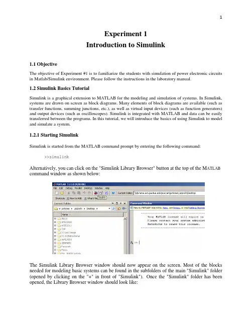
Experiment 1Introduction to Simulink1.1 ObjectiveThe objective of Experiment #1 is to familiarize the students with simulation of power electronic circuits in Matlab/Simulink environment. Please follow the instructions in the laboratory manual.1.2 Simulink Basics TutorialSimulink is a graphical extension to MATLAB for the modeling and simulation of systems. In Simulink, systems are drawn on screen as block diagrams. Many elements of block diagrams are available (such as transfer functions, summing junctions, etc.), as well as virtual input devices (such as function generators) and output devices (such as oscilloscopes). Simulink is integrated with MATLAB and data can be easily transferred between the programs. In this tutorial, we will introduce the basics of using Simulink to model and simulate a system.1.2.1 Starting SimulinkSimulink is started from the MATLAB command prompt by entering the following command: >>simulinkAlternatively, you can click on the "Simulink Library Browser" button at the top of the M ATLAB command window as shown below:The Simulink Library Browser window should now appear on the screen. Most of the blocks needed for modeling basic systems can be found in the subfolders of the main "Simulink" folder (opened by clicking on the "+" in front of "Simulink"). Once the "Simulink" folder has been opened, the Library Browser window should look like:1.2.2 Basic ElementsThere are two major classes of elements in Simulink: blocks and lines. Blocks are used to generate, modify, combine, output, and display signals. Lines are used to transfer signals from one block to another. BlocksThe subfolders underneath the "Simulink" folder indicate the general classes of blocks available for us to use:•Continuous: Linear, continuous-time system elements (integrators, transfer functions, state-space models, etc.)•Discrete: Linear, discrete-time system elements (integrators, transfer functions, state-space models, etc.)•Functions & Tables: User-defined functions and tables for interpolating function values•Math: Mathematical operators (sum, gain, dot product, etc.)•Nonlinear: Nonlinear operators (coulomb/viscous friction, switches, relays, etc.)•Signals & Systems: Blocks for controlling/monitoring signal(s) and for creating subsystems•Sinks: Used to output or display signals (displays, scopes, graphs, etc.)•Sources: Used to generate various signals (step, ramp, sinusoidal, etc.)Blocks have zero to several input terminals and zero to several output terminals. Unused input terminals are indicated by a small open triangle. Unused output terminals are indicated by a small triangular point. The block shown below has an unused input terminal on the left and an unused output terminal on the right.LinesLines transmit signals in the direction indicated by the arrow. Lines must always transmit signals from the output terminal of one block to the input terminal of another block. One exception to this is that a line can tap off of another line. This sends the original signal to each of two (or more) destination blocks, as shown below:Lines can never inject a signal into another line; lines must be combined through the use of a block such as a summing junction.A signal can be either a scalar signal or a vector signal. For Single-Input, Single-Output systems, scalar signals are generally used. For Multi-Input, Multi-Output systems, vector signals are often used, consisting of two or more scalar signals. The lines used to transmit scalar and vector signals are identical. The type of signal carried by a line is determined by the blocks on either end of the line.1.2.3 Building a SystemTo demonstrate how a system is represented using Simulink, we will build the block diagram for a simple model consisting of a sinusoidal input multiplied by a constant gain, which is shown below:This model will consist of three blocks: Sine Wave, Gain, and Scope. The Sine Wave is a Source Block from which a sinusoidal input signal originates. This signal is transferred through a line in the direction indicated by the arrow to the Gain Math Block. The Gain block modifies its input signal (multiplies it by a constant value) and outputs a new signal through a line to the Scope block. The Scope is a Sink Block used to display a signal (much like an oscilloscope).We begin building our system by bringing up a new model window in which to create the block diagram. This is done by clicking on the "New Model" button in the toolbar of the Simulink Library Browser (looks like a blank page).Building the system model is then accomplished through a series of steps:1.The necessary blocks are gathered from the Library Browser and placed in the model window.2.The parameters of the blocks are then modified to correspond with the system we are modeling.3.Finally, the blocks are connected with lines to complete the model.Each of these steps will be explained in detail using our example system. Once a system is built, simulations are run to analyze its behavior.Gathering BlocksEach of the blocks we will use in our example model will be taken from the Simulink Library Browser. To place the Sine Wave block into the model window, follow these steps:1.Click on the "+" in front of "Sources" (this is a subfolder beneath the "Simulink" folder) todisplay the various source blocks available for us to use.2.Scroll down until you see the "Sine Wave" block. Clicking on this will display a shortexplanation of what that block does in the space below the folder list:3. To insert a Sine Wave block into your model window, click on it in the Library Browser and drag the block into your workspace.The same method can be used to place the Gain and Scope blocks in the model window. The "Gain" block can be found in the "Math" subfolder and the "Scope" block is located in the "Sink" subfolder. Arrange the three blocks in the workspace (done by selecting and dragging an individual block to a new location) so that they look similar to the following:Modifying the BlocksSimulink allows us to modify the blocks in our model so that they accurately reflect the characteristics of the system we are analyzing. For example, we can modify the Sine Wave block by double-clicking on it. Doing so will cause the following window to appear:This window allows us to adjust the amplitude, frequency, and phase shift of the sinusoidal input. The "Sample time" value indicates the time interval between successive readings of the signal. Setting this value to 0 indicates the signal is sampled continuously.Let us assume that our system's sinusoidal input has:•Amplitude = 2•Frequency = pi•Phase = pi/2Enter these values into the appropriate fields (leave the "Sample time" set to 0) and click "OK" to accept them and exit the window. Note that the frequency and phase for our system contain 'pi' (3.1415...). These values can be entered into Simulink just as they have been shown.Next, we modify the Gain block by double-clicking on it in the model window. The following window will then appear:Note that Simulink gives a brief explanation of the block's function in the top portion of this window. In the case of the Gain block, the signal input to the block (u) is multiplied by a constant (k) to create the block's output signal (y). Changing the "Gain" parameter in this window changes the value of k.For our system, set k = 5. Enter this value in the "Gain" field, and click "OK" to close the window.The Scope block simply plots its input signal as a function of time, and thus there are no system parameters that we can change for it. We will look at the Scope block in more detail after we have run our simulation.Connecting the BlocksFor a block diagram to accurately reflect the system we are modeling, the Simulink blocks must be properly connected. In our example system, the signal output by the Sine Wave block is transmitted to the Gain block. The Gain block amplifies this signal and outputs its new value to the Scope block, which graphs the signal as a function of time. Thus, we need to draw lines from the output of the Sine Wave block to the input of the Gain block, and from the output of the Gain block to the input of the Scope block.Lines are drawn by dragging the mouse from where a signal starts (output terminal of a block) to where it ends (input terminal of another block). When drawing lines, it is important to make sure that the signal reaches each of its intended terminals. Simulink will turn the mouse pointer into a crosshair when it is close enough to an output terminal to begin drawing a line, and the pointer will change into a double crosshair when it is close enough to snap to an input terminal. A signal is properly connected if its arrowhead is filled in. If the arrowhead is open, it means the signal is not connected to both blocks. To fix an open signal, you can treat the open arrowhead as an output terminal and continue drawing the line to an input terminal in the same manner as explained before.Properly Connected SignalWhen drawing lines, you do not need to worry about the path you follow. The lines will route themselves automatically. Once blocks are connected, they can be repositioned for a neater appearance. This is done by clicking on and dragging each block to its desired location (signals will stay properly connected and will re-route themselves).After drawing in the lines and repositioning the blocks, the example system model should look like:In some models, it will be necessary to branch a signal so that it is transmitted to two or more different input terminals. This is done by first placing the mouse cursor at the location where the signal is to branch. Then, using either the CTRL key in conjunction with the left mouse button or just the right mouse button, drag the new line to its intended destination. This method was used to construct the branch in the Sine Wave output signal shown below:The routing of lines and the location of branches can be changed by dragging them to their desired new position. To delete an incorrectly drawn line, simply click on it to select it, and hit the DELETE key.1.2.4. Running SimulationsNow that our model has been constructed, we are ready to simulate the system. Before starting simulation, we need to set the simulation parameters. To do this, go to the Simulation menu and click on Configuration Parameters. The Configuration Parameters dialog box opens on your desktopEnter desired stop time (e.g. 100 microseconds), and change the Solver Options from Variable-step to fix-step and the step size to 1e-4. The step size specifies the resolution of simulation. Click Apply and OK to close the Configuration Parameters window.Go to the Simulation menu and click on Start, or just click on the "Start/Pause Simulation" button in the model window toolbar (looks like the "Play" button on a VCR). Because our example is a relatively simple model, its simulation runs almost instantaneously. With more complicated systems, however, you will be able to see the progress of the simulation by observing its running time in the lower box of the model window. Double-click the Scope block to view the output of the Gain block for the simulation as a function of time. Once the Scope window appears, click the "Auto scale" button in its toolbar (looks like a pair of binoculars) to scale the graph to better fit the window. Having done this, you should see the following:。

Matlab中文手册目录 (1)第1章MATLAB 6.5环境 (6)1.1 MA TLAB简介 (6)1.1.1 MATLAB工具箱 (6)1.1.2 MATLAB功能和特点 (6)1.2 MA TLAB 6.5环境设置 (7)1.2.1 菜单栏 (7)1.2.2 工具栏 (10)1.2.3 通用操作界面窗口 (10)1.3 MA TLAB 6.5帮助 (19)1.4 MATLAB 6.5其他管理 (20)1.4.1 MATLAB用户文件格式 (20)1.4.2设置搜索路径 (21)1.4.3文件管理命令 (22)1.4.4 退出MA TLAB (23)1.5 一个实例 (23)第2章MATLAB数值计算 (26)2.1 变量和数据 (26)2.1.1数据类型 (26)2.1.2数据 (26)2.1.3变量 (27)2.2 矩阵和数组 (28)2.2.1矩阵输入 (28)2.2.2矩阵元素和操作 (31)2.2.3字符串 (37)2.2.4矩阵和数组运算 (41)2.2.5多维数组 (52)2.3稀疏矩阵 (55)2.3.1稀疏矩阵的建立 (55)2.3.2稀疏矩阵的存储空间 (58)2.3.3稀疏矩阵的运算 (59)2.4多项式 (59)2.4.1多项式的求值、求根和部分分式展开 (59)2.4.2多项式的乘除法和微积分 (61)2.4.3多项式拟合和插值 (63)2.5元胞数组和结构数组 (65)2.5.1元胞数组 (65)2.5.2结构数组 (68)2.6数据分析 (71)2.6.1数据统计和相关分析 (71)2.6.2差分和积分 (72)2.6.3卷积和快速傅里叶变换 (74)2.6.4向量函数 (76)第3章MATLAB符号计算 (77)3.1 符号表达式的建立 (77)3.1.1 创建符号常量 (77)3.1.2 创建符号变量和表达式 (78)3.1.3 符号矩阵 (79)3.2符号表达式的代数运算 (81)3.2.1符号表达式的代数运算 (81)3.2.2 符号数值任意精度控制和运算 (83)3.2.3 符号对象与数值对象的转换 (84)3.3符号表达式的操作和转换 (85)3.3.1符号表达式中自由变量的确定 (85)3.3.2符号表达式的化简 (86)3.3.3符号表达式的替换 (89)3.3.4求反函数和复合函数 (90)3.3.5 符号表达式的转换 (92)3.4 符号极限、微积分和级数求和 (93)3.4.1符号极限 (93)3.4.2符号微分 (94)3.4.3符号积分 (96)3.4.4符号级数 (97)3.5 符号积分变换 (98)3.5.1傅里叶(Fourier)变换及其反变换 (98)3.5.2拉普拉斯(Laplace)变换及其反变换 (99)3.5.3 Z变换及其反变换 (100)3.6符号方程的求解 (101)3.6.1代数方程 (101)3.6.2符号常微分方程 (102)3.7符号函数的可视化 (103)3.7.1符号函数的绘图命令 (103)3.7.2图形化的符号函数计算器 (105)3.8 Maple函数的使用 (105)3.8.1访问Maple函数 (105)3.8.2 获得Maple的帮助 (106)第4章MA TLAB计算的可视化和GUI设计 (107)4.1二维曲线的绘制 (107)4.1.1基本绘图命令plot (107)4.1.2绘制曲线的一般步骤 (111)4.1.3多个图形绘制的方法 (112)4.1.4曲线的线型、颜色和数据点形 (114)4.1.5设置坐标轴和文字标注 (115)4.2 MA TLAB的三维图形绘制 (119)4.2.1绘制三维线图命令plot3 (119)4.2.2绘制三维网线图和曲面图 (120)4.2.3立体图形与图轴的控制 (123)4.2.4色彩的控制 (125)4.3 MA TLAB的特殊图形绘制 (128)4.3.1条形图 (128)4.3.2面积图和实心图 (129)4.3.3直方图 (130)4.3.4饼图 (131)4.3.5离散数据图 (132)4.3.6对数坐标和极坐标图 (132)4.3.7等高线图 (133)4.3.8复向量图 (134)4.4图形窗口的功能 (135)4.5对话框 (136)4.6句柄图形 (138)4.6.1句柄图形体系 (138)4.6.2图形对象的操作 (139)4.6.3图形对象属性的获取和设置 (142)4.7图形用户界面(GUI)设计 (144)4.7.1可视化的界面环境 (144)4.7.2菜单 (145)4.7.3控件 (146)4.7.5回调函数 (148)4.7.6 GUI应用举例 (148)4.8动画 (151)4.8.1以电影方式产生动画 (151)4.8.2以对象方式产生动画 (151)第5章MATLAB程序设计 (153)5.1脚本文件和函数文件 (153)5.1.1 M文本编辑器 (153)5.1.2 M文件的基本格式 (153)5.1.3 M脚本文件 (154)5.1.4 M函数文件 (155)5.2程序流程控制 (156)5.2.1 for ... end循环结构 (156)5.2.2 while ... end循环结构 .. (157)5.2.3 If...else...end条件转移结构 (158)5.2.4 switch...case开关结构 (158)5.2.5 try... catch... end试探结构 . (160)5.2.6流程控制语句 (160)5.3函数调用和参数传递 (162)5.3.2局部变量和全局变量 (163)5.3.3函数的参数 (164)5.3.4程序举例 (167)5.4 M文件性能的优化和加速 (169)5.4.1 P码文件 (169)5.4.2 M文件性能优化 (169)5.4.3 JIT和加速器 (170)5.5内联函数 (173)5.6利用函数句柄执行函数 (174)5.6.1函数句柄的创建 (174)5.6.2用feval命令执行函数 (175)5.7利用泛函命令进行数值分析 (176)5.7.1求极小值 (177)5.7.2求过零点 (178)5.7.3数值积分 (179)5.7.4微分方程的数值解 (179)第6章线性控制系统分析与设计 (181)6.1线性系统的描述 (181)6.1.1状态空间描述法 (181)6.1.2传递函数描述法 (182)6.1.3零极点描述法 (183)6.1.4离散系统的数学描述 (183)6.2线性系统模型之间的转换 (186)6.2.1连续系统模型之间的转换 (186)6.2.2连续系统与离散系统之间的转换 (189)6.2.3模型对象的属性 (192)6.3结构框图的模型表示 (194)6.4线性系统的时域分析 (202)6.4.1零输入响应分析 (202)6.4.2脉冲响应分析 (203)6.4.3阶跃响应分析 (204)6.4.4任意输入的响应 (205)6.4.5系统的结构参数 (207)6.5线性系统的频域分析 (208)6.5.1频域特性 (208)6.5.2连续系统频域特性 (209)6.5.3幅值裕度和相角裕度 (212)6.5.4离散系统频域分析 (213)6.6线性系统的根轨迹分析 (213)6.6.1绘制根轨迹 (213)6.6.2根轨迹的其它工具 (215)6.7线性系统的状态空间设计 (218)6.7.1极点配置法 (218)第7章Simulink仿真环境 (220)7.1演示一个Simulink的简单程序 (220)7.2 Simulink的文件操作和模型窗口 (222)7.2.1 Simulink的文件操作 (222)7.2.2 Simulink的模型窗口 (222)7.3 模型的创建 (224)7.3.1模块的操作 (224)7.3.2信号线的操作 (226)7.3.3给模型添加文本注释 (227)7.4 Simulink的基本模块 (227)7.4.1基本模块 (227)7.4.2常用模块的参数和属性设置 (229)7.5复杂系统的仿真与分析 (232)7.5.1仿真的设置 (232)7.5.2连续系统仿真 (233)7.5.3离散系统仿真 (236)7.5.4仿真结构参数化 (238)7.6子系统与封装 (238)7.6.1建立子系统 (238)7.6.2条件执行子系统 (240)7.6.3子系统的封装 (241)7.7用MA TLAB命令创建和运行Simulink模型 (245)7.7.1用MA TLAB命令创建Simulink模型 (245)7.7.2用MA TLAB命令运行Simulink模块 (247)7.8以Simulink为基础的模块工具箱简介 (248)第8章MA TLAB高级应用 (248)8.1 MA TLAB应用接口 (248)8.1.1 MEX文件 (248)8.1.2 使用MA TLAB编译器生成MEX和EXE文件 (252)8.2 低级文件的输入输出 (254)8.2.1打开和关闭文件 (254)8.2.2读写格式化文件 (255)8.2.3读写二进制数据 (257)8.2.4文件定位 (258)8.3 图形文件的转储 (260)8.4 Notebook (260)8.4.1 Notebook的安装 (260)8.4.2 Notebook的启动 (261)8.4.3 Notebook的使用 (262)8.4.4 Notebook中MA TLAB的使用 (265)第1章MATLAB 6.5环境1.1MATLAB简介●MATLAB(Matrix Laborator)是MathWorks公司开发科学与工程计算软件；●广泛应用于自动控制、数学运算、信号分析、计算机技术、图像信号处理、财务分析、航天工业、汽车工业、生物医学工程、语音处理和雷达工程等行业；●国内外高校和研究部门科学研究的重要工具；●MATLIB 已成为数学计算工具方面事实上的标准，MATLIB 6.5是最新版本。

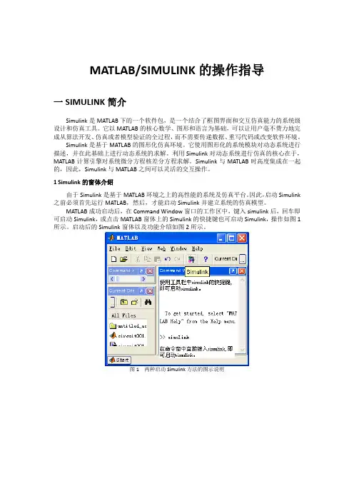
MATLAB/SIMULINK的操作指导一SIMULINK简介Simulink是MATLAB下的一个软件包，是一个结合了框图界面和交互仿真能力的系统级设计和仿真工具。

它以MATLAB的核心数学、图形和语言为基础，可以让用户毫不费力地完成从算法开发、仿真或者模型验证的全过程，而不需要传递数据、重写代码或改变软件环境。

Simulink是基于MATLAB的图形化仿真环境。

它使用图形化的系统模块对动态系统进行描述，并在此基础上进行动态系统的求解。

利用Simulink对动态系统进行仿真的核心在于，MATLAB计算引擎对系统微分方程核差分方程求解。

Simulink与MATLAB时高度集成在一起的，因此，Simulink与MATLAB之间可以灵活的交互操作。

1 Simulink的窗体介绍由于Simulink是基于MATLAB环境之上的高性能的系统及仿真平台。

因此，启动Simulink 之前必须首先运行MATLAB，然后，才能启动Simulink并建立系统的仿真模型。

MATLAB成功启动后，在Command Window窗口的工作区中，键入simulink后，回车即可启动Simulink，或点击MATLAB窗体上的Simulink的快捷键也可启动Simulink，操作如图1所示。

启动后的Simulink窗体以及功能介绍如图2所示。

图1 两种启动Simulink方法的图示说明图.2 Simulink库浏览器窗口2 一个MATLAB/Simulink库自代的演示实例MATLAB/Simulink自代了大量的演示实例，为读者创建模型提供许多有益的帮助，读者可借鉴这些实例。

浏览演示实例可在Command Window窗的工作区键入demo回车即可，或点击MATLAB窗体的左下角的Start按钮也可浏览，选择出所需的模型。

线性电路的暂态分析模型如图3所示，其运行结果如图.4所示。

图 3 线性电路暂态分析的演示仿真模型图.4 线性电路暂态分析的演示仿真模型的运行结果3 创建一个MATLAB实例对Simulink库有了初步了解后，创建一个简单电路的仿真模型并运行。

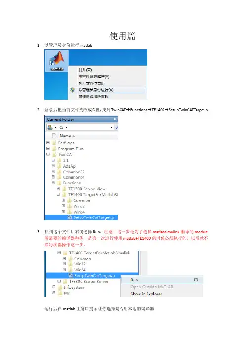
使用篇1.以管理员身份运行matlab2.登录后把当前文件夹改成C盘，找到TwinCAT→Functions→TE1400→SetupTwinCATTarget.p3.找到这个文件后右键选择Run，注意：这一步是为了选择matlabsimulink编译的module所需要的编译器种类，是第一次运行使用matlab+TE1400的时候必须执行的，以后就不必每次都操作这一步。

运行后在matlab主窗口提示让你选择是否用本地的编译器因为本地有VS2010的编译器，所以选择y后敲回车随后matlab找到本地有两种编译器，一个是matlab本体的lcc-win32 C2.4.1，另一个是VS2010，选择VS2010所代表的数字，输入2敲回车最后让matlab让你确认编译器的选择，输入y敲回车提示以下信息说明编译器选择完成4.点击工具栏中simulink图标5.弹出simulink编辑界面后，点击工具栏中的打开模型6.找到案例模型TempContrTest.mdl，点击打开7.本次案例模型是一个简单的温度控制External Setpoint是设定温度Feedback Temp是当前温度CoolerON是开关量输出8.打开simulation菜单栏，选择configuration parameters进行参数设定（1）进入参数设定后，选择右边的树形栏中的Solver，把其中的Type改成Fixed-step（2）之后选择树形栏中的Code Generation，把其中的System target file改成TwinCAT.tlc 点击Browse可以进行选择（3）继续选择树形栏中的Tc Module，在Publish module和Publish binaries for platform “TwinCAT RealTime（x86）”前打勾（4）最后选择树形栏中的Tc Advanced，把Task assignment改成Default在Add to cyclic caller，Variable cycle time，Export block digram以及Export block diagram debug information前打勾（5）以上操作完成后点击左下角的Apply（6）选择树形栏中的Code Generation，把Generate code only勾选后点击Generate code，随后matlab就开始把这个模型通过TE1400生成TC3所识别的Module了（7）回到matlab主窗口，等看到以下提示说明Module生成完成（8）我们来看下生成的Module会在什么位置可以发现在TwinCAT/3.1/CustomConfig/Modules路径下会生成名字和案例模型名字一样的文件夹TempContrTest打开可以发现里面其实主要是.tmc文件是TC3所需要的，其他都是一些描述文件，所以可以把.tmc文件拷贝出来，给一些没有Matlab的电脑上用9.打开TC3，并新建项目10.把名称改成英文，例如matlabsimulink，点击确认11.打开SYSTEM，右键TcCOM Objects添加新项12.TC3会自动找到之前生成的.tmc文件，选中后点击OK进行添加13.添加好后我们可以发现TcCOM Objects下出现matlab生成的Module，并且3个变量出现在IO位置，方便和PLC程序或者硬件IO进行变量连接14.右键Tasks添加新项名字可以改成matlab，点击OK添加新的Task15.因为我需要实施做温度计算，所以可以这个Task的优先级提高，修改成1，周期用默认的10ms即可16.双击TcCOM Objects下面的Object1（TempContrTest）Depend On改成Manual Config，并把Task分配成之前创建的名为“matlab”的Task17.右键PLC添加新项18.把名称修改为英文，例如test19.编辑一段模拟程序，模拟温度的升降20.程序写好后右键test Project，选择生成开始编译程序21.编译好后在test Instance自动生成3个变量22.接下来要做的就是把PLC中3个变量和matlab中三个变量链接起来Switch→CoolerONSP→External SetpointPV Feedback Temp23.变量链接完成后开始下传配置和程序，选择菜单栏TwinCAT，点击Activate Configuration弹出窗口点击确定提示切换到运行模式点击确定观察右下角图标是否编程绿色运行状态弹出窗口点击确定提示切换到运行模式点击确定观察右下角图标是否编程绿色运行状态24.打开PLC菜单，选择“登录到”把程序在线25.打开PLC菜单，选择“启动”把程序运行26.观察程序，看到成功利用matlab温度算法运行程序27.打开Object1（TempContrTest），选择Block Diagram也可以同时观察Matlab温度算法实时状态注：上图中可以看到由一个红色字提示说是非商业的，虽然TE1400插件装上了，但用的还是7天试用版，所以对于试用版有一些限制，查询information system可以看到如下：TC3中Scope View简单使用在之前的基础上来看下TC3下Scope View如何使用，装好TC3后Scope View会自动集成在TC3中1.首先右键“解决方案”选择添加，点击新建项目2.选择TwinCAT Measurement中的Measurement Scope Project，名称改成英文，例如tempcontrol，点击确定3.右键Axis，选择Target Browser4.打开小电脑图标下的Port_851(851)，点击MAIN5.把MAIN程序中PV和SP分别添加到同一个坐标上6.保证程序在运行后，点击工具栏中的Record开始记录两个变量7.随后就可以观察到当前PV和SP的示波图下图中绿色是PV，蓝色是SP。

精品Simulink中文帮助Simulink可以对实际的动态系统建模，仿真并实时分析系统输出的变化。

利用Simulink仿真动态系统分两步：1，用户创建一个结构框图，利用Simulink模型编辑器，通过系统的输入，传递函数，输出描述数学关系2，仿真系统的模型，并指定开始时间和结束时间二、Simulink动态系统建模仿真结构图是动态系统数学模型的图形化描述，数学模型由一组方程组表示，包括比例，微分，微分方程。

创建动态系统模型的要素用户可以用Simulink软件包建模、仿真和分析模型输出随时间而改变的系统，这样的系统通常是指动态系统：利用Simulink，用户可以搭建很多领域的动态系统，包括电子电路、减振器、刹车系统和许多其他的电子、机械和热力学系统。

使用Simulink仿真动态系统包括两个过程。

首先，利用Simulink的模型编辑器创建被仿真系统的模型方块图，系统模型描述了系统中输入、输出、状态和时间的数学关系，然后使用Simulink根据用户输入的模型信息在一个时间段内仿真动态系统。

本节综合给出了用户在Simulink中创建动态系统模型时需要理解和掌握的所有建模要素。

1方块图Simulink方块图是动态系统数学模型的图形化描述，动态系统的数学模型是由一组方程来表示的，而由方块图模型所描述的数学方程就是众所周知的代数方程、微分方程和(或)差分方程。

方块图模型中的每个模块都属于一个特定的Simulink模块类型，模块的类型决定了模块的输出、输入、状态与时间的关系，在建立系统模型图时，Simulink方块图中可以包含任意数目、任意类型的模块，Simulink中的模块包括非虚拟模块和虚拟模块。

非虚拟模块是基本系统，虚拟模块则是为了模型方块图组织结构的简化而建立的，它在模型方块图所描述的系统方程定义中不起任何作用、如BuCreator模块和BuSelector模块就是虚拟模块，它们的作用只是把信号\捆绑\在一起用来简化方块图，而且也增加了模型的可读性。

Matlab中文手册目录 ................................................................................................................... 错误!未定义书签。

第1章MATLAB 6.5环境 ............................................................................ 错误!未定义书签。

1.1 MA TLAB简介 .................................................................................... 错误!未定义书签。

1.1.1 MATLAB工具箱 ..................................................................... 错误!未定义书签。

1.1.2 MATLAB功能和特点 ............................................................. 错误!未定义书签。

1.2 MA TLAB 6.5环境设置 ...................................................................... 错误!未定义书签。

1.2.1 菜单栏...................................................................................... 错误!未定义书签。

1.2.2 工具栏...................................................................................... 错误!未定义书签。

第1章MATLAB 6.5环境1.1MATLAB简介●MATLAB(Matrix Laborator)是MathWorks公司开发科学与工程计算软件；●广泛应用于自动控制、数学运算、信号分析、计算机技术、图像信号处理、财务分析、航天工业、汽车工业、生物医学工程、语音处理和雷达工程等行业；●国内外高校和研究部门科学研究的重要工具；●MATLIB 已成为数学计算工具方面事实上的标准，MATLIB 6.5是最新版本。

1.1.1 MATLAB工具箱●MATLAB由基本部分和功能各异的工具箱组成。

基本部分是MATLAB的核心，工具箱是扩展部分。

●工具箱是用MATLAB的基本语句编成的各种子程序集，用于解决某一方面的专门问题或实现某一类的新算法。

●MATLAB有以下主要的工具箱：▪控制系统工具箱(Control System Toolbox)▪系统辨识工具箱(System Identification Toolbox)▪信号处理工具箱(Signal Processing Toolbox)▪神经网络工具箱(Neural Network Toolbox)▪模糊逻辑控制工具箱(Fuzzy Logic Toolbox)▪小波工具箱(Wavelet Toolbox)▪模型预测控制工具箱(Model Predictive Control Toolbox)▪通信工具箱(Communication Toolbox)▪图像处理工具箱(Image Processing Toolbox)▪频域系统辨识工具箱(Frequency System Identification Toolbox)▪优化工具箱(Optimization Toolbox)▪偏微分方程工具箱(Partial Differential Equation Toolbox)▪财政金融工具箱(Financial Toolbox)▪统计工具箱(Statistics Toolbox)1.1.2 MATLAB功能和特点1．功能强大(1) 运算功能强大●MATLAB的数值运算要素不是单个数据，而是矩阵，每个元素都可看作复数，运算包括加、减、乘、除、函数运算等；●通过MATLAB的符号工具箱，可以解决在数学、应用科学和工程计算领域中常常遇到的符号计算问题。

使用篇1.以管理员身份运行matlab2.登录后把当前文件夹改成C盘，找到TwinCAT→Functions→TE1400→SetupTwinCATTarget.p3.找到这个文件后右键选择Run，注意：这一步是为了选择matlabsimulink编译的module所需要的编译器种类，是第一次运行使用matlab+TE1400的时候必须执行的，以后就不必每次都操作这一步。

运行后在matlab主窗口提示让你选择是否用本地的编译器因为本地有VS2010的编译器，所以选择y后敲回车随后matlab找到本地有两种编译器，一个是matlab本体的lcc-win32 C2.4.1，另一个是VS2010，选择VS2010所代表的数字，输入2敲回车最后让matlab让你确认编译器的选择，输入y敲回车提示以下信息说明编译器选择完成4.点击工具栏中simulink图标5.弹出simulink编辑界面后，点击工具栏中的打开模型6.找到案例模型TempContrTest.mdl，点击打开7.本次案例模型是一个简单的温度控制External Setpoint是设定温度Feedback Temp是当前温度CoolerON是开关量输出8.打开simulation菜单栏，选择configuration parameters进行参数设定（1）进入参数设定后，选择右边的树形栏中的Solver，把其中的Type改成Fixed-step（2）之后选择树形栏中的Code Generation，把其中的System target file改成TwinCAT.tlc 点击Browse可以进行选择（3）继续选择树形栏中的Tc Module，在Publish module和Publish binaries for platform “TwinCAT RealTime（x86）”前打勾（4）最后选择树形栏中的Tc Advanced，把Task assignment改成Default在Add to cyclic caller，Variable cycle time，Export block digram以及Export block diagram debug information前打勾（5）以上操作完成后点击左下角的Apply（6）选择树形栏中的Code Generation，把Generate code only勾选后点击Generate code，随后matlab就开始把这个模型通过TE1400生成TC3所识别的Module了（7）回到matlab主窗口，等看到以下提示说明Module生成完成（8）我们来看下生成的Module会在什么位置可以发现在TwinCAT/3.1/CustomConfig/Modules路径下会生成名字和案例模型名字一样的文件夹TempContrTest打开可以发现里面其实主要是.tmc文件是TC3所需要的，其他都是一些描述文件，所以可以把.tmc文件拷贝出来，给一些没有Matlab的电脑上用9.打开TC3，并新建项目10.把名称改成英文，例如matlabsimulink，点击确认11.打开SYSTEM，右键TcCOM Objects添加新项12.TC3会自动找到之前生成的.tmc文件，选中后点击OK进行添加13.添加好后我们可以发现TcCOM Objects下出现matlab生成的Module，并且3个变量出现在IO位置，方便和PLC程序或者硬件IO进行变量连接14.右键Tasks添加新项名字可以改成matlab，点击OK添加新的Task15.因为我需要实施做温度计算，所以可以这个Task的优先级提高，修改成1，周期用默认的10ms即可16.双击TcCOM Objects下面的Object1（TempContrTest）Depend On改成Manual Config，并把Task分配成之前创建的名为“matlab”的Task17.右键PLC添加新项18.把名称修改为英文，例如test19.编辑一段模拟程序，模拟温度的升降20.程序写好后右键test Project，选择生成开始编译程序21.编译好后在test Instance自动生成3个变量22.接下来要做的就是把PLC中3个变量和matlab中三个变量链接起来Switch→CoolerONSP→External SetpointPV Feedback Temp23.变量链接完成后开始下传配置和程序，选择菜单栏TwinCAT，点击Activate Configuration弹出窗口点击确定提示切换到运行模式点击确定观察右下角图标是否编程绿色运行状态弹出窗口点击确定提示切换到运行模式点击确定观察右下角图标是否编程绿色运行状态24.打开PLC菜单，选择“登录到”把程序在线25.打开PLC菜单，选择“启动”把程序运行26.观察程序，看到成功利用matlab温度算法运行程序27.打开Object1（TempContrTest），选择Block Diagram也可以同时观察Matlab温度算法实时状态注：上图中可以看到由一个红色字提示说是非商业的，虽然TE1400插件装上了，但用的还是7天试用版，所以对于试用版有一些限制，查询information system可以看到如下：TC3中Scope View简单使用在之前的基础上来看下TC3下Scope View如何使用，装好TC3后Scope View会自动集成在TC3中1.首先右键“解决方案”选择添加，点击新建项目2.选择TwinCAT Measurement中的Measurement Scope Project，名称改成英文，例如tempcontrol，点击确定3.右键Axis，选择Target Browser4.打开小电脑图标下的Port_851(851)，点击MAIN5.把MAIN程序中PV和SP分别添加到同一个坐标上6.保证程序在运行后，点击工具栏中的Record开始记录两个变量7.随后就可以观察到当前PV和SP的示波图下图中绿色是PV，蓝色是SP。