Part V Prototype Documentation for the Performance Prediction Component Delivery Slip Name
- 格式:pdf
- 大小:1.05 MB
- 文档页数:28
制作模型的步骤英语作文Title: Steps in Creating a Model。
Model-making is a fascinating process that involves creativity, precision, and attention to detail. Whetheryou're building a scale model of a historical landmark or crafting a prototype for a scientific experiment, there are several key steps to follow to ensure a successful outcome. In this essay, we will explore the essential steps involved in creating a model.1. Define the Purpose: The first step in model-makingis to clearly define the purpose of the model. Ask yourself: What is the model intended to represent or demonstrate? Understanding the purpose will guide all subsequent decisions throughout the process.2. Research and Planning: Once the purpose is established, thorough research is necessary. Gather information about the subject matter, including dimensions,colors, textures, and any other relevant details. With this information, create a detailed plan outlining the materials needed, the scale of the model, and the overall design.3. Material Selection: Selecting the appropriate materials is crucial for the success of the model. Consider factors such as durability, ease of manipulation, and suitability for the intended purpose. Common materials for model-making include wood, plastic, foam, clay, and various types of adhesives.4. Prototype Creation (if applicable): In some cases, especially in scientific or engineering projects, it may be necessary to create a prototype before constructing the final model. Prototyping allows for testing and refinement of design concepts before committing to the full-scale model.5. Construction: With the plan in place and materials gathered, it's time to start constructing the model. Follow the design carefully, paying close attention to measurements and proportions. Use appropriate tools andtechniques for cutting, shaping, and assembling the materials.6. Detailing and Finishing: Adding details is what brings a model to life. Whether it's painting, applying decals, adding textures, or incorporating miniature elements, the devil is in the details. Take your time to ensure precision and accuracy in every aspect of the finishing touches.7. Quality Control: Before considering the model complete, perform a thorough quality control check. Inspect for any flaws, imperfections, or inaccuracies that may detract from the overall appearance or functionality of the model. Make necessary adjustments as needed.8. Presentation and Display: How the model is presented and displayed can greatly impact its effectiveness. Consider the intended audience and purpose when deciding on the presentation format. Whether it's a museum exhibit, a scientific demonstration, or a classroom project, ensure the model is displayed in a manner that highlights its keyfeatures.9. Documentation: Finally, document the process of creating the model. This documentation serves as a valuable reference for future projects and allows others to learn from your experiences. Include details such as materials used, techniques employed, challenges faced, and lessons learned.In conclusion, model-making is a multifaceted process that requires careful planning, precise execution, and attention to detail. By following these essential steps, you can create models that are not only visually impressive but also effective in achieving their intended purpose. Whether you're a hobbyist, a student, or a professional, mastering the art of model-making opens up a world of creative possibilities.。
本科毕业论文(设计)外文翻译外文题目International Accounting Standard 38Intangible Assets外文出处IASCF38 Pages857-859外文作者 International Accounting Standards Board (IASB) 原文:International Accounting Standard 38Intangible Assets Objective1 The objective of this Standard is to prescribe the accounting treatment for intangible assets that are not dealt with specifically in another Standard. This Standard requires an entity to recognise an intangible asset if, and only if, specified criteria are met. The Standard also specifies how to measure the carrying amount of intangible assets and requires specified disclosures about intangible assets.Scope2 This Standard shall be applied in accounting for intangible assets, except:(a) intangible assets that are within the scope of another Standard;(b) financial assets, as defined in IAS 32 Financial Instruments: Presentation;(c) the recognition and measurement of exploration and evaluation assets (see IFRS 6 Exploration for and Evaluation of Mineral Resources);(d) expenditure on the development and extraction of minerals, oil, natural gasand similar non-regenerative resources.3 If another Standard prescribes the accounting for a specific type of intangible asset, an entity applies that Standard instead of this Standard. For example, this Standard does not apply to:(a) intangible assets held by an entity for sale in the ordinary course of business (see IAS 2 Inventories and IAS 11 Construction Contracts).(b) deferred tax assets (see IAS 12 Income Taxes).(c) leases that are within the scope of IAS 17 Leases.(d) assets arising from employee benefits (see IAS 19 Employee Benefits).(e) financial assets as defined in IAS 32. The recognition and measurement of some financial assets are covered by IAS 27 Consolidated and Separate Financial Statements, IAS 28 Investments in Associates and IAS 31 Interests in Joint Ventures.(f) goodwill acquired in a business combination (see IFRS 3 Business Combinations).(g) deferred acquisition costs, and intangible assets, arising from an insurer’s contractual rights under insurance contracts within the scope of IFRS 4 Insurance Contracts. IFRS 4 sets out specific disclosure requirements for those deferred acquisition costs but not for those intangible assets. Therefore, the disclosure requirements in this Standard apply to those intangible assets.(h) non-current intangible assets classified as held for sale (or included in a disposal group that is classified as held for sale) in accordance with IFRS 5 Non-current Assets Held for Sale and Discontinued Operations.4 Some intangible assets may be contained in or on a physical substance such asa compact disc (in the case of computer software), legal documentation (in the case of a licence or patent) or film. In determining whether an asset that incorporates both intangible and tangible elements should be treated under IAS 16 Property, Plant and Equipment or as an intangible asset under this Standard, an entity uses judgement to assess which element is more significant. For example, computer software for a computer-controlled machine tool that cannot operate without that specific software is an integral part of the related hardware and it is treated as property, plant and equipment. The same applies to the operating system of a computer. When the software is not an integral part of the related hardware, computer software is treated as an intangible asset.5 This Standard applies to, among other things, expenditure on advertising, training, start-up, research and development activities. Research and development activities are directed to the development of knowledge. Therefore, although theseactivities may result in an asset with physical substance (eg a prototype), the physical element of the asset is secondary to its intangible component, ie the knowledge embodied in it.6 In the case of a finance lease, the underlying asset may be either tangible or intangible. After initial recognition, a lessee accounts for an intangible asset held under a finance lease in accordance with this Standard. Rights under licensing agreements for items such as motion picture films, video recordings, plays, manuscripts, patents and copyrights are excluded from the scope of IAS 17 and are within the scope of this Standard.7 Exclusions from the scope of a Standard may occur if activities or transactions are so specialised that they give rise to accounting issues that may need to be dealt with in a different way. Such issues arise in the accounting for expenditure on the exploration for, or development and extraction of, oil, gas and mineral deposits in extractive industries and in the case of insurance contracts. Therefore, this Standard does not apply to expenditure on such activities and contracts. However, this Standard applies to other intangible assets used (such as computer software), and other expenditure incurred (such as start-up costs), in extractive industries or by insurers.Definitions8 The following terms are used in this Standard with the meanings specified:An active market is a market in which all the following conditions exist:(a) the items traded in the market are homogeneous;(b) willing buyers and sellers can normally be found at any time;(c) prices are available to the public.Amortisation is the systematic allocation of the depreciable amount of an intangible asset over its useful life.An asset is a resource:(a) controlled by an entity as a result of past events;(b) from which future economic benefits are expected to flow to the entity.Carrying amount is the amount at which an asset is recognised in the statement of financial position after deducting any accumulated amortisation and accumulatedimpairment losses thereon.Cost is the amount of cash or cash equivalents paid or the fair value of other consideration given to acquire an asset at the time of its acquisition or construction, or, when applicable, the amount attributed to that asset when initially recognised in accordance with the specific requirements of other IFRSs, eg IFRS 2 Share-based Payment.Depreciable amount is the cost of an asset, or other amount substituted for cost, less its residual value.Development is the application of research findings or other knowledge to a plan or design for the production of new or substantially improved materials, devices, products, processes, systems or services before the start of commercial production or use.Entity-specific value is the present value of the cash flows an entity expects to arise from the continuing use of an asset and from its disposal at the end of its useful life or expects to incur when settling a liability.Fair value of an asset is the amount for which that asset could be exchanged between knowledgeable, will ing parties in an arm’s length transaction.An impairment loss is the amount by which the carrying amount of an asset exceeds its recoverable amount.An intangible asset is an identifiable non-monetary asset without physical substance.Monetary assets are money held and assets to be received in fixed or determinable amounts of money.Research is original and planned investigation undertaken with the prospect of gaining new scientific or technical knowledge and understanding.The residual value of an intangible asset is the estimated amount that an entity would currently obtain from disposal of the asset, after deducting the estimated costs of disposal, if the asset were already of the age and in the condition expected at the end of its useful life.Useful life is:(a) the period over which an asset is expected to be available for use by an entity;(b) the number of production or similar units expected to be obtained from the asset by an entity.Intangible assets9 Entities frequently expend resources, or incur liabilities, on the acquisition, development, maintenance or enhancement of intangible resources such as scientific or technical knowledge, design and implementation of new processes or systems, licences, intellectual property, market knowledge and trademarks (including brand names and publishing titles). Common examples of items encompassed by these broad headings are computer software, patents, copyrights, motion picture films, customer lists, mortgage servicing rights, fishing licences, import quotas, franchises, customer or supplier relationships, customer loyalty, market share and marketing rights.10 Not all the items described in paragraph 9 meet the definition of an intangible asset, ie identifiability, control over a resource and existence of future economic benefits. If an item within the scope of this Standard does not meet the definition of an intangible asset, expenditure to acquire it or generate it internally is recognised as an expense when it is incurred. However, if the item is acquired in a business combination, it forms part of the goodwill recognised at the acquisition date (see paragraph 68).DisclosureGeneral118 An entity shall disclose the following for each class of intangible assets, distinguishing between internally generated intangible assets and other intangible assets:(a) whether the useful lives are indefinite or finite and, if finite, the useful lives or the amortisation rates used;(b) the amortisation methods used for intangible assets with finite useful lives;(c) the gross carrying amount and any accumulated amortisation (aggregated with accumulated impairment losses) at the beginning and end of the period;(d) the line item(s) of the statement of comprehensive income in which any amortisation of intangible assets is included;(e) a reconciliation of the carrying amount at the beginning and end of the period showing:(i) additions, indicating separately those from internal development, those acquired separately, and those acquired through business combinations;(ii) assets classified as held for sale or included in a disposal group classified as held for sale in accordance with IFRS 5 and other disposals;(iii) increases or decreases during the period resulting from revaluations under paragraphs 75, 85 and 86 and from impairment losses recognised or reversed in other comprehensive income in accordance with IAS 36 (if any);(iv) impairment losses recognised in profit or loss during the period in accordance with IAS 36 (if any);(v) impairment losses reversed in profit or loss during the period in accordance with IAS 36 (if any);(vi) any amortisation recognised during the period;(vii) net exchange differences arising on the translation of the financial statements into the presentation currency, and on the translation of a foreign operation into the presentation currency of the entity;(viii) other changes in the carrying amount during the period.119 A class of intangible assets is a grouping of assets of a similar nature and use in an entity’s operations. Examples of separa te classes may include:(a) brand names;(b) mastheads and publishing titles;(c) computer software;(d) licences and franchises;(e) copyrights, patents and other industrial property rights, service and operating rights;(f) recipes, formulae, models, designs and prototypes;(g) intangible assets under development.The classes mentioned above are disaggregated (aggregated) into smaller (larger) classes if this results in more relevant information for the users of the financial statements.120 An entity discloses information on impaired intangible assets in accordance with IAS 36 in addition to the information required by paragraph 118(e)(iii)–(v).121 IAS 8 requires an entity to disclose the nature and amount of a change in an accounting estimate that has a material effect in the current period or is expected to have a material effect in subsequent periods. Such disclosure may arise from changes in:(a) the assessment of an intangible asset’s useful life;(b) the amortisation method;(c) residual values.122 An entity shall also disclose:(a) for an intangible asset assessed as having an indefinite useful life, the carrying amount of that asset and the reasons supporting the assessment of an indefinite useful life. In giving these reasons, the entity shall describe the factor(s) that played a significant role in determining that the asset has an indefinite useful life.(b) a description, the carrying amount and remaining amortisation period of any individual intangible asset that is material to the entity’s financial statements.(c) for intangible assets acquired by way of a government grant and initially recognised at fair value (see paragraph 44):(i) the fair value initially recognised for these assets;(ii) their carrying amount;(iii) whether they are measured after recognition under the cost model or the revaluation model.(d) the existence and carrying amounts of intangible assets whose title is restricted and the carrying amounts of intangible assets pledged as security for liabilities.(e) the amount of contractual commitments for the acquisition of intangible assets.123 When an entity describes the factor(s) that played a significant role in determining that the useful life of an intangible asset is indefinite, the entity considers the list of factors in paragraph 90.Intangible assets measured after recognition using the revaluation model124 If intangible assets are accounted for at revalued amounts, an entity shall disclose the following:(a) by class of intangible assets:(i) the effective date of the revaluation;(ii) the carrying amount of revalued intangible assets;(iii) the carrying amount that would have been recognised had the revalued class of intangible assets been measured after recognition using the cost model in paragraph 74;(b) the amount of the revaluation surplus that relates to intangible assets at the beginning and end of the period, indicating the changes during the period and any restrictions on the distribution of the balance to shareholders;(c) the methods and significant a ssumptions applied in estimating the assets’ fair values.125 It may be necessary to aggregate the classes of revalued assets into larger classes for disclosure purposes. However, classes are not aggregated if this would result in the combination of a class of intangible assets that includes amounts measured under both the cost and revaluation models.Foreign source:International Accounting Standards Board (IASB) .International Accounting Standard38—Intangible Assets.IASCF38.2003:857-859.译文:国际会计准则第38 号无形资产目的1.本准则的目的是对其他国际会计准则中没有具体涉及的无形资产的会计处理进行规范。
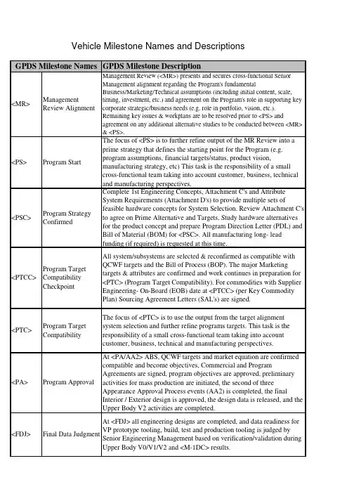
GPDS Milestone Description<MR>ManagementReview AlignmentManagement Review (<MR>) presents and secures cross-functional SeniorManagement alignment regarding the Program's fundamentalBusiness/Marketing/Technical assumptions (including initial content, scale,timing, investment, etc.) and agreement on the Program's role in supporting keycorporate strategic/business needs (e.g. role in portfolio, vision, etc.).Remaining key issues & workplans are to be resolved prior to <PS> andagreement on any additional alternative studies to be conducted between <MR>& <PS>.<PS>Program Start The focus of <PS> is to further refine output of the MR Review into a prime strategy that defines the starting point for the Program (e.g. program assumptions, financial targets/status, product vision, manufacturing strategy, etc) This task is the responsibility of a small cross-functional team taking into account customer, business, technical and manufacturing perspectives.<PSC>Program StrategyConfirmedComplete 1st Engineering Concepts, Attachment C's and AttributeSystem Requirements (Attachment D's) to provide multiple sets offeasible hardware concepts for System Selection. Review Attachment C'sto agree on Prime Alternative and Targets. Study hardware alternativesfor the product concept and prepare Program Direction Letter (PDL) andBill of Material (BOM) for <PSC>. All manufacturing long- leadfunding (if required) is requested at this time.<PTCC>Program TargetCompatibilityCheckpointAll system/subsystems are selected & reconfirmed as compatible withQCWF targets and the Bill of Process (BOP). The major Marketingtargets & attributes are confirmed and work continues in preparation for<PTC> (Program Target Compatibility). For commodities with SupplierEngineering- On-Board (EOB) date at <PTCC> (per Key CommodityPlan) Sourcing Agreement Letters (SAL's) are signed.<PTC>Program TargetCompatibilityThe focus of <PTC> is to use the output from the target alignmentsystem selection and further refine programs targets. This task is theresponsibility of a small cross-functional team taking into accountcustomer, business, technical and manufacturing perspectives.<PA>Program Approval At <PA/AA2> ABS, QCWF targets and market equation are confirmed compatible and become objectives, Commercial and Program Agreements are signed, program objectives are approved, preliminary activities for mass production are initiated, the second of three Appearance Approval Process events (AA2) is completed, the final Interior / Exterior design is approved, the design data is released, and the Upper Body V2 activities are completed.<FDJ>Final Data Judgment At <FDJ> all engineering designs are completed, and data readiness for VP prototype tooling, build, test and production tooling is judged by Senior Engineering Management based on verification/validation during Upper Body V0/V1/V2 and <M-1DC> results.Vehicle Milestone Names and Descriptions GPDS Milestone Names<VP>VerificationPrototypeThe VP builds are production intent for all Underbody and Upper Bodycontent, including UP electrical, and P/T calibration. The VP ProgramPDL (Feature/Options Summary) is defined at <PTC>. The VP Prototypecontent is defined to efficiently satisfy specific DV test requirements.The VP Digital Pre-Assembly (DPA) prototype variants are aligned tophysical builds. DPA ensures vehicle compatibility and designcompleteness. A VP Electrical Engineering Breadboard build is required,and the Electrical Design Completion timing is identified on programVPP. GPDS v2.2 maximizes production / hard tooling for the VP andlater builds phases.<PEC>PreliminaryEngineeringCompletionThe Preliminary Engineering Completion (PEC) event includes all the documentationand signatory elements described within FAP 03-201. Preliminary EngineeringCompletion is an engineering gateway where Senior Engineering Management assessesthe status of Program versus attribute and financial objectives. The intent of PEC is toidentify shortfalls to objectives and to confirm work plans are in place to successfullyachieve Final Engineering Completion (FEC). Success criteria are described in FAP 03-201.<FEC>Final EngineeringCompletionAt <FEC> Final Engineering Completion is authorized by SeniorManagement based upon the successful completion of all designvalidation testing and confirmation of no major open issues/risks.<LR>Launch Readiness At <LR> all Verification Prototype (VP) issues are resolved, all cross-functional activities' readiness to proceed to Body Construction / Assembly Tooling Trial is confirmed, and final approval to proceed to Tooling Trial is obtained.<LS>Launch Sign-off Pilot Production (PP) Approval is the approval to proceed to the PP build. Approval is obtained at the Launch Sign-Off Meeting, in which the following should occur: determine the readiness of internal & external tooling/equipment and operator training etc. for each relevant department; forecast the achievement level of quality targets; and Confirm and provide External Supplier APQP/PPAP Readiness –Element Summary Report (Schedule B). All data previously stated is required to proceed to PP.<J1>Job #1The physical product / process functional evaluation is conducted; homologation /self certification (excluding US Emissions) is performed, body & vehicle pilot production (PP) is completed, and approval to proceed to MP1 is obtained.<OKTB>Okay To Buy Okay-To-Buy confirms MP2 quality confirmation results, & vehicle static/drive evaluations. The Okay-To-Buy meeting is held at the Assembly Plant. The meeting should be held around the product with a follow up discussion of the measurables from the Okay-to-Buy scorecard. The discussion of the measurables will be given by the responsible launch team/assembly plant members who will present the recommendations and the decision/facts that are reported on the Okay-to-Buy scorecard.Prototype Builds Final Status ReportAn initial summary is prepared after MP (Mass Production) team events. The ProgramManagement team confirms program objective achievement status, identifies countermeasures, documents final results/lessons learned (financials, sales & market share,quality surveys, campaigns, field actions, etc.) and obtains approval for the final report.DescriptionPrototype BuildsFC0FeasibilityCheckpoint 0The Studio Feasibility Process is a subset of GPDS deliverables and astep by step guide for Design & surface development. Prior to <FC0>,Annual Process and Advanced (pre PS) activities are taking place tosupport the initial program assumptions. At FC0, only a small team ofdesigners and engineers are working on the project to establish a set ofhigh level program assumptions. Resulting from the outputs of pre PSactivities, at <FC0> the Concept Design is decided.FC1FeasibilityCheckpoint 1The Studio Feasibility Process is a subset of GPDS deliverables and astep by step guide for Design & surface development. At FC1,Functional Engineering and Design Studio completes benchmarking.Additionally, mechanical & occupant package parameters are beingestablished. The Studio Design Theme alternatives are evaluated againstprogram assumptions and attribute strategies. Representations of selectedStudio Design Theme alternatives are prepared to support the plannedPackage & Concept Clinic.FC2FeasibilityCheckpoint 2The Studio Feasibility Process is a subset of GPDS deliverables and astep by step guide for Design & surface development. At FC2, the threeStudio Design alternatives are matured along with the programassumptions. Functional Engineering completes Attachment C/Dreconciliation allowing provisional upper body system selection. StudioDesign Theme alternatives are assessed to attribute target ranges.FC3FeasibilityCheckpoint 3The Studio Feasibility Process is a subset of GPDS deliverables and astep by step guide for Design & surface development. At FC3, the threeStudio Design alternatives are matured and further refined until Themesare narrowed down to 2 with Character Feasibility completed (+/-10mmto +/-20mm).FC4FeasibilityCheckpoint 4The Studio Feasibility Process is a subset of GPDS deliverables and a step by step guidefor Design & surface development. At FC4, along with the results from the Theme &Package Clinic, the Studio Design Theme is evaluated against program assumptions andattribute point targets. Cost checkpoint to collect supplier data has been added forversion 2.2.FC5FeasibilityCheckpoint 5The Studio Feasibility Process is a subset of GPDS deliverables and a step by step guidefor Design & surface development. From FC4 to FC5, the Single Design Theme isfurther refined with additional feasibility inputs incorporated. Preliminary upper bodygeometry is available for program team evaluation. Exterior and interior math surfacedata reflecting Design intent is provided to the program team. FC5 represents the end ofDesign led change.AA1AppearanceApproval 1At <AA1> the first of three Appearance Approval Process events iscompleted, approval for Interior and Exterior Design feasible surfaces isobtained, and the transfer of production intent surfaces and the start ofUpper Body V2 activities is initiated.AA2AppearanceApproval 2From AA1 to AA2, all surface data files are released from the DesignStudio to the program team. Digital Pre Assembly activity continues.AA1 marks the beginning of surface release. <AA2> represents the endof surface release. Releases are phased depending on part ranking.FAA Final AppearanceApprovalAt <FAA> the final event in the Appearance Approval process iscompleted, Interior / Exterior surface final refinements and highlights areapproved, and supporting design data is updated.DescriptionX-1X-1 Prototype First Drivable X-1 Prototype Vehicle build is completed and ready to be delivered to the customer.M-1M-1 Prototype First Drivable M-1 Prototype Vehicle build is completed and ready to be delivered to the customer. M-1 vehicles are used to verify key specifications in the Under Body area.DescriptionUNV0Underbody V0DevelopmentDuring this phase engineers collect information and develop Under Bodybase mechanical package work plan. Information includes: <PSC>program paper, pre-V0 mechanical package data, 1st engineeringconcept, Attachment C and preliminary vehicle & system attribute targetranges (Attachment D), and then develop mechanical package work plan.UNV1Underbody V1DevelopmentDuring this phase engineers update the Underbody V1 Geometric 2D/3Dprogram intent CAD data, non-geometric data, and engineering databased upon latest 3D data, digital pre-assembly reviews,system/component CAE assessments, Campaign Prevention actions andVO resolution actions.UNV2Underbody V2DevelopmentDuring this phase engineers confirm and refine V2 UnderbodySystem/Component designs and Mechanical Package to achieve allapplicable vehicle level engineering requirements and PMT targets. ForAgreed Exception ‘Long Lead’ tools, tool order may be placed prior toUNV2 and rough cutting of tools may start at the completion of UNV2(not before).M-1DJ M-1 Data Judgment At M1-DJ all Underbody engineering designs are completed, and the data is ready for release for M1 prototype tooling, build and test. Final cutting of tools may start at the completion of M1DJ (not before). The goal is to complete supplier testing by M-1 MRD. On an exception basis for agreed ‘long lead’ parts some aspects of component testing may be allowed to complete post MRD provided the integrity of the vehicle build and test plan is not judged to be compromised. Each commodity team must define the critical component testing which must be completed prior to M1 MRD and get signed off as part of the M1DJ sign-offUPV0Upperbody V0DevelopmentDuring this phase engineers collect information and develop Upper Bodybase mechanical package work plan. Information includes: <PSC>program paper, pre-V0 mechanical package data, 1st engineeringconcept, Attachment C and preliminary vehicle & system attribute targetranges (Attachment D), and then develop mechanical package work plan.Prototype Builds Engineering GatewaysUPV1Upperbody V1DevelopmentDuring this phase engineers update the Upperbody V1 Geometric 2D/3Dprogram intent CAD data, non-geometric data, and engineering databased upon latest 3D data, digital pre-assembly reviews,system/component CAE assessments, Campaign Prevention actions andVO resolution actions.UPV2Upperbody V2DevelopmentDuring this phase engineers confirm and refine V2 UpperbodySystem/Component designs and Mechanical Package to achieve allapplicable vehicle level engineering requirements and PMT targets. ForAgreed Exception ‘Long Lead’ tools, tool order may be placed prior toUPV2 and rough cutting of tools may start at the completion of UPV2(not before).M-1DC M-1 DevelopmentCompleteCompile the <M-1DC> Engineering Sign Off Report (targetdemonstration versus status). All Program risks for Quality, Cost,Weight, & Functional Targets assessed and countermeasures developed.Identify and select the M-1 Drive Vehicle. Prepare M-1 Drive Vehicleand schedule the M-1 SME Drive. Conduct the attribute characterizationof the M-1 Drive Vehicle. Develop work plan and countermeasures toclose issues identified during <M-1DC> testing and M-1 Drive VehiclePreparation.DescriptionTT Tooling Trial –Build StartThe Tooling Trial (TT) Vehicles Built per Pre-Launch Control Plan is abuild conducted at the production location utilizing production tooling,process, and hard-tooled production parts at the required PPAP level(LQOS Standard G06). The build is conducted per the Pre-ProductionControl Plan to verify capability of assembly production tools,equipment, facilities & processes to ensure readiness for Pilot Production(PP).PP Pilot Production –Build StartThe readiness and the ability to proceed for Pilot Production is assessed,the start of Pilot Production is authorized, the MP1 readiness isreviewed, and Pre-production builds are conducted to verify thecapability of the production tools, equipment, facilities, systems andprocesses with hard-tooled production parts.MP1Mass Production 1MP1 Vehicles Built per Production Control Plan is a build verifying the compatibility of production process, facilities, and tooling with material at the required PPAP level (LQOS Standard G06). MP1 Build Review Meeting, in which the following should occur: confirm the readiness of internal & external tooling/equipment and operator training etc. for each relevant department is complete; confirm the achievement level of quality to targets Confirm and provide External Supplier APQP/PPAP Readiness –Element Summary Report (Schedule B). All data previously stated is required to proceed to MP2.MP2Mass Production 2MP2 Vehicles Built to Production Control Plan is a build verifying the compatibility of production process, facilities, and tooling with material at the required PPAP level (Standard G06).Assembly Plant Build Starts。

[Legal entity Supplier], [Place of Registration/ Headquarter] [VAT Number/ Registration Number][Country][Legal entity of Continental Corporation][Place of Registration/ Headquarter][Country]DesignationGeneral Quality Agreement Rev. BDocument key PagesTable of ContentsPage1 Introduction 3 1.1 1.2 DefinitionsParties to this agreement 3 3 1.3 Scope3 1.4 Background / Area of Application 4 1.5 Validity4 2 General System Requirements5 2.1 2.2 Management System Requirements SupplyOn usage5 5 2.3 Sub-Supplier Control 5 2.4 Audits5 2.5 Supplier Performance Indicators and Rating6 2.6 Escalation Process7 2.7 Record Retention / Archiving Period 8 2.8 Design for environment 8 2.9 Contingency plans8 3 Advanced Quality Planning9 3.1 Feasibility Commitment, Supplier Component Review (SCR) 9 3.2 Advanced Product Quality Planning (APQP) 9 3.3 Engineering Prototype Sample Submissions 9 3.4 FMEA9 3.5 3.6 Measurement System Analysis (MSA) Special Characteristics 10 10 3.7 Qualification11 3.8 Manufacturing Process Review11 3.9 Production Part Approval Process (PPAP) 11 3.10 Product and Process Release Information 12 4 Ramp up Process13 4.1 Pre-Production and Sample Part Requirements 13 4.2 Safe Launch Concept 13 5 Serial Production14 5.1 Deviation Approval for Product or Process Deviations 14 5.2 Process Capability and Control 14 5.3 Annual Re-Qualification 15 5.4 Certificates of Conformance 15 5.5 Problem Solving Methods15 5.6 Non Conforming Components / Corrective Actions16 5.7 Changes to Approved Products and Processes (PCN) 16 5.8 Identification and traceability 16 5.9 5.10 Incoming Inspection Shelf-Life 17 17 6 Reference18 7 8 Reference to ISO/TS 16949 Abbreviations19 20 9 Record of Changes 21DesignationGeneral Quality Agreement Rev. BDocument keyPages1.Introduction1.1Definitions“Party” or “Parties” shall mean individually or collectively Continental and/or Supplier, or any Participating Related Company/Companies individually or as contracting parties to an agreement concluded pursuant to this GQA, as the case may be.1.2 Parties to this agreementThis GQA shall apply to the Parties including the Participating Related Companies of the Parties. Related Companies shall mean any company which, through ownership of voting stock or otherwise, directly or indirectly, is controlled by, under the common control with, or in control of a Party hereto, the term "control" meaning the ownership of more than 50 % of such company's voting rights.Related Companies may accede to, become bound by, and avail themselves of the rights and remedies of this GQA by signing or otherwise entering an Individual Agreement. Such Participating Related Company shall then be bound mutatis mutandis as Continental and Supplier by the terms and conditions of this GQA as having entered into the GQA by itself.For the avoidance of doubt, a Participating Related Company will not become jointly and severally liable for the obligations of any other Party or Participating Related Company.1.3 ScopeThe purpose of this document is to communicate Continental requirements with respect to the quality and environmental management system of those companies that supply production goods and/or services to Continental.It is the Suppliers’ obligation to ensure that all quality rules set out in this Agreement are transmitted, implemented and committed to by the members of Supplier’s sub-supplier panel. Continental expects zero defects for every quoted contract-product and a commitment from our Suppliers to implement appropriate systems and controls to ensure the 100% on-time delivery of conforming, defect free products.DesignationGeneral Quality Agreement Rev. BDocument keyPages1.4Background / Area of ApplicationContinental Supplier Quality and Environmental System Requirements are based upon the latest edition of ISO/TS 16949 Quality System Requirements and ISO 14001 Environmental System Requirements. Although this does not alter or reduce any other requirements of the contract, it is intended to provide a concise understanding of our quality and environmental expectations. By signing this GQA the Supplier hereby acknowledges that this GQA applies to all components and services supplied by him to any Continental location world-wide.1.5 ValidityAs of the Effective Date this GQA embodies all the terms and conditions of the contract between the Parties with respect to the subject matter hereof and supersedes and cancels all previous agreements and understandings. There are no verbal statements which have not been embodied herein.Relevant incorporated documents (see Annex 1) shall become applicable with signature of the GQA. New or revised incorporated documents will be provided via the SupplyOn service “Document Manager”. They become valid if there is no objection received in writing within a three month period from the facility for taking notice of the documents.In case of conflicting rules between the rules of this Agreement and any other agreement/ document, the order of precedence of the documents is as follows: 1. Strategic Supplier Contract 2. Component specification / drawing 3. General Quality Agreement (GQA)(i) Category Quality Requirements (ii) Quality Process Requirements (iii) Continental General Specifications 4. Sourcing Agreement 5. Purchase OrderDeviations from the order of precedence are possible if the Parties expressly agree to deviate in individual agreements and reflect that agreement by adding the following wording to each provision: “The following provision shall apply in expressed deviation to Chapter… of the …”DesignationGeneral Quality Agreement Rev. BDocument keyPages2.General System Requirements2.1 Management System RequirementsPresent and potential suppliers to Continental must operate within a comprehensive quality system. Suppliers shall provide written confirmation and objective evidence of third party certification to an active version of ISO/TS 16949. Suppliers who are not ISO/TS 16949 (latest issue) certified must have a working plan to become compliant to ISO/TS 16949 available for review, unless the supplier has an approved exemption from Continental waiving such a plan.Suppliers are required to install environmental systems in their facilities that are compliant to ISO 14001. Suppliers who are not certified must have a working plan to become compliant to ISO 14001 available for review, unless the supplier has an approved exemption from Continental waiving such a plan.Certified suppliers must record their initial and renewal certifications in the “Business Directory” of the SupplyOn Platform within 10 days of receiving the certificate from their registrar.2.2 SupplyOn usageSupplier shall register to SupplyOn and actively use the following services: Sourcing, Document Manager, Performance Monitor, Project Management, Problem Solver.2.3Sub-Supplier ControlThe requirements set out in this Agreement shall also apply to the QM-System that the Supplier shall set up with its sub-suppliers. Upon Continental’s request the Supplier shall submit supplier- and product approvals and corresponding quality contracts with its sub-suppliers. The Supplier shall notify Continental of any changes to their approved Supplier list and request Continental’s approval following the rules set force in Chapter 5.7 (PCN). Each supplier is responsible for the control and continuous improvement efforts of sub-suppliers. That responsibility as well applies to sub-suppliers nominated by Continental. Suppliers shall enable visits by Continental at their suppliers.2.4 AuditsUpon request Continental, a 3rd party representative or customers shall be entitled to visit any product related location of the Supplier and to conduct audits based on ISO/TS 16949 and VDA standards. This right shall also include audits at the Supplier’s sub-suppliers’ locations. The Supplier shall provide the necessary resources for the performance of this task. The Supplier is, however, not obligated to reveal any proprietary information without a mutual non-disclosure-agreement in place.DesignationGeneral Quality Agreement Rev. BDocument keyPagesA scoring and audit report will be provided by the respective auditor at the end of an audit during the common wrap-up discussion with the involved participants. The audit report and the necessary measures resulting from the audit (as far as identifiable) shall be agreed upon by the Supplier and Continental within an action plan. The tracking and follow-up for the realization of the action plan will be performed by Continental's auditor.Each year, the Supplier shall perform a self audit according to VDA 6.3 standard for all product lines including subcontracted processes. Continental shall be informed of all audit results below 85% or C classification. Upon request of Continental the Supplier shall provide all audit results including documentation and action plans.Clause 8.2.2.2 of ISO/TS 16949:2002 require that the organization shall audit each manufacturing process to determine its effectiveness. Self-Assessments by the suppliers including any sub-supplied parts or outsourced processes to be applied in accordance to AIAG Special Processes (CQI). Continental Automotive requires that applicable audits are conducted at minimum frequency of once per year and that record of assessments including action plans be maintained and made available to Continental SQM upon request. Compliance to be demonstrated for the latest edition of following special processes:• CQI-9 : Heat Treat Assessment (HTSA) • CQI-11 : Plating System Assessment (PSA) • CQI-12 : Coating System Assessment (CSA) • CQI-15 : Welding System Assessment (WSA) •CQI-17 : Soldering System Assessment (SSA)2.5Supplier Performance Indicators and RatingContinental performs a supplier evaluation in several categories based on key performance indicators such as: IncidentsAn Incident is any significant and product or component relevant disturbance generated by a supplier influencing Continental or a Continental customer. An incident is equal to one quality notification (QN) which is created in case of:• Customer Complaints Field/Warranty • Customer Complaints 0-km• Continental Productions Complaints• Continental Incoming Inspection Complaints •Continental Logistics complaintsPPM-LevelThe PPM-Level evaluates the Supplier’s performance in parts per million for failures at Continental incoming inspection, Continental manufacturing line and customer defects.DesignationGeneral Quality Agreement Rev. BDocument keyPagesAPQP performanceFor the definition of APQP requirements see chapter 3.2.The performance will be measured based on the fulfillment of mandatory elements.Cycle timeCycle time is the calculated response time (in days) of the Supplier to a complaint issued by Continental. Requirements see “Quality Process Requirements for Complaint Management (QPR A2C00052917AAA).8D Quality8D Quality is rated using the 8D evaluation systematic described in “Quality Process Requirements for Complaint Management (QPR A2C00052917AAA).Supplier EvaluationThe global performance of the Supplier will be evaluated annually for purchasing, quality, logistics and technology elements and serves to determine Continental strategic supply base.Based on the results of such evaluation the Supplier shall define and implement appropriate corrective actions. If the quality results fail to meet the committed goals, the Supplier shall implement immediate corrective actions to reach the targets.2.6 Escalation ProcessAn escalation process is launched in case of non satisfying Supplier performance.The Supplier shall enable a visit from Continental or a meeting within 48 hours after receipt of the complaint.Incident escalationAs entry criteria into the escalation an 8D report from the Supplier is mandatory. Based on the 8D report and an expert meeting the supplier could be set to CSL1 in order to prevent re-occurrence of the same failure.In case of CSL1 the Supplier shall apply additional / redundant testing to prevent shipping of non-conforming components to Continental. The testing process shall include a 100% screening. The screening shall be applied to all components at the Supplier's location, in transit, or at Continental's plant.CSL2 may be applied independently from CSL1, the application of CSL2 shall be mandatory if a failed part is delivered during CSL1. In case of CSL2 the Supplier shall hire an independent thirdDesignationGeneral Quality Agreement Rev. BDocument keyPagesParty approved by Continental which needs to perform the containment actions and to support the related 8D process.Components shipped under CSL1 or CSL2 shall be marked with a mutually agreed upon identification method.Worst supplier escalationAs entry criteria into the escalation an action plan from the Supplier is mandatory. Based on the action plan and an expert meeting the Supplier could be set to CSL1. If there is no progress concerning the actions agreed, a management meeting shall be conducted and based on the results the supplier could be set to CSL2.CSL1 or CSL 2 can be used as containment action.A Q-BIC@supplier program can be launched to support the improvement plan. Top Management Meeting, New Business on Hold, Phase-OutIn case that CSL1/2 failed or the VDA6.3 audit result has been ranked with C or the supplier evaluation results have been insufficient, a Top Management Meeting will be organized. The output of the meeting could lead to the decision "New Business on Hold" or "Phase-Out".2.7 Record retentionThe Supplier shall be obligated to document and maintain Production Part Approval Process (PPAP) documentation, annual layout and validation records, tooling records, traceability records, engineering records, corrective action records, quality performance records and inspection and test results. In minimum the listed documents shall be archived over at least 15 years after Continental production has been terminated and tooling scrap authorization has been granted. Records shall be available to Continental upon request. The above time periods are considered “minimum”. All retention times shall meet or exceed the above requirements and any governmental requirements.2.8 Design for EnvironmentSuppliers are obligated to contribute to the implementation for environmental requirements in product design. Requirements which must be met by the Suppliers under aspect of product-related protection of the environment are set force in Continentals Quality Process Requirements “Design for Environment of Purchased Components and Modules" (QPR A2C00909200AAA).2.9 Contingency plansSuppliers are required to prepare contingency plans (e.g. facility interruptions, labor shortages, key equipment failure and field returns) to reasonably protect Continental's supply of product in the event of an emergency, excluding Acts of God / Force Majeure.DesignationGeneral Quality Agreement Rev. BDocument keyPages3.Advanced Quality Planning3.1 Feasibility Commitment, Supplier Component Review (SCR)With each offer to Continental, the Supplier shall submit a feasibility commitment in regards to project time plan, quality targets and technical requirements. The Supplier shall perform a detailed feasibility analysis and present the outcome during a "Supplier Component Review Meeting". The main output of this meeting will be a feasibility commitment to a common agreed project time schedule, a common agreed (target) specification/drawing and a fixed supply chain.3.2 Advanced Product Quality Planning (APQP)Supplier and its sub-suppliers shall have a comprehensive APQP process in place in accordance to the latest AIAG and Continental’s requirements. Suppliers shall maintain APQP using the SupplyOn service “Project Management” for each component development project. Based on these requirements Continental has the opportunity to verify the APQP process at the Supplier as well as at the sub-supplier's premises together with its customer. The Supplier shall have a designated project engineer / manager for each component development project, who will be available upon request by Continental to be part of the overall project team.3.3 Engineering Prototype Sample SubmissionEngineering prototype parts with documentation of specification conformance shall be submitted to Continental by the supplier as instructed by the department at Continental responsible for prototype and engineering validation testing. Each sample or prototype must be clearly labeled as such and accompanied by completed dimensional results, material test results, and performance test results reports as described in the AIAG PPAP Manual. Specific instructions, in addition to these stated requirements, may be agreed upon and documented by Continental via the APQP Kick-Off Meeting or other formal communication.3.4 FMEAThe Supplier shall conduct FMEAs before design and process validation in accordance to AIAG standard. FMEAs shall:(a) recognize and evaluate the potential failure modes of the design & process as well aseffects of failure modes,(b) identify actions that could eliminate or reduce the chance of the potential failure occurring,and(c) document the entire process.All identified potential failure modes shall be considered in order to improve the product & process. Supplier shall set up a rating system in its QM-system which identifies the priorities of recommended measures (e.g. RPN, Severity).DesignationGeneral Quality Agreement Rev. BDocument keyPagesThe first release of each FMEA shall be transmitted to Continental before design validation and process qualification. Each event or change shall be updated in such FMEAs.The process FMEA shall be delivered to Continental, the design FMEA shall be made available for review.3.5 Measurement System AnalysisThe Supplier shall perform Measurement System Analysis (MSA) studies according latest AIAG MSA Manual for all gauges and measurement systems/equipments indicated in respective Control Plans for qualification, pre-series and production components. Each MSA study need to cover Gage R&R, bias, linearity and stability studies and need to demonstrate that percentage Gauge R&R (%GRR) < 10% with a “number of distinct categories” (ndc) ≥ 5.In case the %GRR is between > 10% and < 30% or ndc < 5 the Supplier has to implement corrective actions. Usage of such marginal measurement systems requires Continental’s approval. %GRR > 30% shall not be used for manufacturing of Continental components at any time.The herein specified MSA requirements need to be assured by the Supplier during the complete component life cycle this includes changes like e.g. product changes, process changes, measurement system changes, measurement system repairs or any other change which could influence the performance of the measurement system.3.6Special CharacteristicsSpecial Characteristics are any product characteristics defined by Continental or customers or manufacturing process parameters identified by the Supplier including government and safety regulations, which have a substantial influence on the:- manufacturability at Continental - manufacturability at the customer- usage and operation of the product by the customer - compliance with applicable regulations-compliance to applicable safety requirementsSpecial Characteristics are further categorized into:- Characteristics not relating to safety or legal considerations -Characteristics with safety or legal considerationsDesignationGeneral Quality Agreement Rev. BDocument keyPagesIn accordance with the requirements of ISO/TS 16949, Special Characteristics shall be identified and specifically addressed in the Design-FMEA, Process-FMEA, Control Plans, Process Flows, work instructions and other associated documents.Continental required Special Characteristics will be identified on drawings/specifications or in a separate document that cross-references these characteristics to the drawings/specifications. The supplier is responsible to fully understand the process impact to their product and identify any process parameter Special Characteristics as they deem appropriate. Suppliers are also responsible for ensuring that relevant Special Characteristics are explained, understood and controlled by their sub-suppliers where applicable.3.7 QualificationThe Supplier shall maintain a qualification system for processes and components which are capable of proving the requirements as defined in the respective specifications/drawings and incorporated documents (see Annex 1).3.8 Manufacturing Process ReviewThe Supplier is responsible to carry out reviews in his area of responsibility. They must be scheduled in such a way that the results are available on the specified release days (milestones) of the project. An assessment of a supplier’s manufacturing process may be conducted before and after part approval at the supplier’s facility. This assessment may be specified by Continental or its customer (e.g. Run@Rate and VDA 6.3 Audit).3.9 Production Part Approval Process (PPAP)The Supplier shall conduct the PPAP according to the date specified. PPAP shall determine whether all Continental engineering design requirements, specification requirements and process requirements are met by the Supplier and that the process has the defined capability to produce components meeting these requirements during an actual production run at the quoted production rate.PPAP shall be performed following the rules set out in the AIAG PPAP manual and related Continental requirements.The standard PPAP submission level shall be 3, unless otherwise agreed.Upon request by Continental, the PPA requirements as referenced in the VDA volume 2 manual shall be used.PPAPs shall be submitted to the requesting quality department and any associated PPAP sample parts shall be clearly labeled as such.DesignationGeneral Quality Agreement Rev. BDocument keyPages3.10 Product- and Process Release InformationThe Component and Process is released after a PSW has been countersigned by Continental SQM. Changes of the process or component are not allowed after this point without prior notification. Supplier’s components shall not be accepted by Continental for series production in case a product release has not been issued. Any production shipments received by Continental prior to obtaining a countersigned PSW will be rejected. The PSW does not constitute Application- or Manufacturing approval at Continental. In case a full approval cannot be achieved on time a written deviation approval is required prior to shipping parts to Continental for production. Continental shall inform the Supplier of such product release. .DesignationGeneral Quality Agreement Rev. BDocument keyPages4.Ramp up Process4.1 Pre-Production and Sample Part requirementsSuppliers are required to meet Continental's Pre-production and Sample Part requirements. These requirements will be defined by Continental via the APQP Kick-Off Meeting or other formal communication. Required documentation (e.g. Control Plans) must be kept current.Suppliers are expected to clearly identify “pre-production” or “sample parts” to ensure that Continental's receiving site does not mix such parts with “regular” production parts. Suppliers are also expected to work closely with Continental plant Scheduling and Material Control personnel to minimize unnecessary obsolescence. Labeling must be done per Continental's receiving site requirements and shall be differentiated from regular production shipping labels, unless the parts are already PPAP approved. In particular, the Supplier Identification, Part Number, Engineering Level, and Quantity must be clearly displayed on the part-packaging label to ensure easy, visible segregation of containers/parts.4.2 Safe Launch ConceptThe Supplier shall apply a Safe Launch Concept (SLC) according to the product and process maturity. The scale of the SLC shall be defined during the APQP process and agreed by Continental. The purpose of the SLC is to document the Supplier's control of its processes during start-up and ramp-up phase, it shall also enable the Supplier to quickly identify and quickly correct any quality issues that may arise at the Supplier's location. SLC includes special verifications performed by the Supplier for a defined timeframe or quantity as determined together with Continental in the APQP process.SLC requires a Pre-Launch Control Plan, which is a significant enhancement to the Supplier's production control plan and which in turn will raise the confidence level to ensure that all components shipped initially will meet Continental's expectations. The Pre-launch control plan will also serve to validate the production control plan. The Pre-Launch Control Plan shall take into consideration all known critical conditions of the product as determined with Continental as well as potential areas of concerns in the Supplier’s process as also identified during the introduction and PPAP. The Supplier shall generate the Pre-Launch Control Plan prior to start of series production and shall make it available to Continental for approval prior to start of series production. Continental shall be entitled to request changes.Suppliers are required to submit inspection data to Continental's plant. This should include variable measurement data where applicable. Suppliers may exit the safe launch process if they have achieved SLC targets unless otherwise specified by Continental.DesignationGeneral Quality Agreement Rev. BDocument keyPagesSuppliers shall develop action plans to address missed failure modes or capability improvement needs. Continental may require suppliers to perform production on stock for product and process verification purpose. Missing achievement of the SLC targets within the mutual defined period of time or quantities may lead to a withdrawal of the release.5.Serial Production5.1 Deviation Approval for Product or Process DeviationsIt is the policy of Continental not to accept products that do not meet the requirements of the applicable drawings and specifications. Requests for deviations on nonconforming products shall be submitted to Continental's receiving plant for review and approval prior to shipment. Deviations shall be approved only for a specific time period or quantity of parts. No permanent deviations are permitted. A deviation request shall be accompanied by a Problem Solving Report (8D). This report shall include the identification of a clean point and the manner in which products will be identified, including how traceability will be maintained.5.2 Process Capability and ControlSuppliers are required that processes shall meet process capability and SPC requirements as defined in the AIAG PPAP and SPC reference manual, unless otherwise specified by Continental Automotive. The acceptance criteria for short term studies is a Cmk and Ppk >= 2. For long term process capability a Cpk >= 1,67 is required.The supplier is responsible that control requirements are documented in the control plan and that capability indices are achieved and improved throughout production. If the required capability cannot be reached then 100% testing is mandatory.The Supplier is obligated to define samples ("golden" samples) to be used as reference for the manufacturing process and final product.Upon request of Continental the Supplier shall provide measurement and traceability data for special characteristics.The Supplier shall inform Continental about any deviation of the current reading of the First Pass Yield (FPY) from the average weekly FPY of more than +/-10% for any product within two days after the deviation occurred. The Supplier shall provide information regarding the current and past FPY upon request of Continental.Without the prior written approval of Continental the Supplier shall not repair or sort components. Rework/repair includes all activities on components outside the documented process flow.。

TECHNICAL ISO/TS SPECIFICATION 16949质量管理体系-汽车生产件和相关服务件组织应用ISO 9001:2008的特别要求Quality management systems -Particular requirements for the applicationof ISO 9001:2008 for automotive productionand relevant service part organizationsReference numberISO/TS 16949:2009 (E)© ISO 2009ContentsForewordRemarks for certificationIntroduction0.1 General总则0.2 Process approach过程方法0.3 Relationship with ISO 9004 与ISO 9004的关系0.3.1 IATF Guidance to ISO/TS 16949:2002 IATF关于ISO/TS 16949:2002的指南0.4 Compatibility with other management systems与其他管理体系的相容性0.5 Goal of this Technical Specification本技术规范的目标1 Scope范围1.1 General总则1.2 Application应用2 Normative reference规范性引用文件3 Terms and definitions术语和定义3.1Terms and definitions for the automotive industry汽车行业的术语和定义4 Quality management system 质量管理体系4.1 General requirements 总要求4.1.1 General requirements – Supplemental 总要求-补充4.2 Documentation requirements 文件要求4.2.1 General总则4.2.2 Quality manual质量手册4.2.3 Control of documents 文件控制4.2.3.1 Engineering specifications 工程规范4.2.4 Control of records 记录控制4.2.4.1 Records retention 记录保存5 Management responsibility管理职责5.1 Management commitment管理承诺5.1.1 Process efficiency过程效率5.2 Customer focus以顾客为关注焦点5.3 Quality policy 质量方针5.4 Planning策划5.4.1 Quality objectives质量目标5.4.1.1 Quality objectives – Supplemental 质量目标-补充5.4.2 Quality management system planning质量管理体系策划5.5 Responsibility, authority and communication职责权限与沟通5.5.1 Responsibility and authority 职责和权限5.5.1.1 Responsibility for quality质量职责5.5.2 Management representative管理者代表5.5.2 1 Customer representative顾客代表5.5.3 Internal communication内部沟通5.6 Management review管理评审5.6.1 General总则5.6.1.1 Quality management system performance 质量管理体系绩效5.6.2 Review input 评审输入5.6.2.1 Review input – Supplemental 评审输入-补充5.6.3 Review output评审输出6 Resource management 资源管理6.1 Provision of resources资源提供6.2 Human resources人力资源6.2.1 General总则6.2.2 Competence, awareness and training and awareness 能力、意识和培训和意识6.2.2.1 Product design skills 产品设计技能6.2.2.2 Training 培训6.2.2.3 Training on the job 岗位培训6.2.2.4 Employee motivation and empowerment 员工激励和授权6.3 Infrastructure 基础设施6.3.1 Plant, facility and equipment planning 工厂、设施和设备策划6.3.2 Contingency plans 应急计划6.4 Work environment 工作环境6.4.1 Personnel safety to achieve conformity to product quality requirements与实现产品质量要求符合性相关的人员安全6.4.2 Cleanliness of premises 生产现场的清洁7 Product realization 产品实现7.1 Planning of product realization产品实现的策划7.1.1 Planning of product realization – Supplemental 产品实现的策划-补充7.1.2 Acceptance criteria 接收准则7.1.3 Confidentiality 保密7.1.4 Change control 更改控制7.2 Customer-related processes 与顾客有关的过程7.2.1 Determination of requirements related to the product与产品有关的要求的确定7.2.1.1 Customer-designated special characteristics 顾客指定的特殊特性7.2.2 Review of requirements related to the product与产品有关的要求的评审7.2.2.1 Review of requirements related to the product - Supplemental与产品有关的要求的评审-补充7.2.2.2 Organization manufacturing feasibility 组织制造可行性7.2.3 Customer communication 顾客沟通7.2.3.1 Customer communication – Supplemental顾客沟通-补充7.3 Design and development 设计和开发7.3.1 Design and development planning 设计和开发策划7.3.1.1 Multidisciplinary approach 多方论证方法7.3.2 Design and development inputs 设计和开发输入7.3.2.1 Product design input 产品设计输入7.3.2.2 Manufacturing process design input 制造过程设计输入7.3.2.3 Special characteristics 特殊特性7.3 3 Design and development outputs 设计和开发输出7.3.3.1 Product design outputs – Supplemental 产品设计输出-补充7.3.3.2 Manufacturing process design output制造过程设计输出7.3.4 Design and development review 设计和开发评审7.3.4.1 Monitoring 监视7.3.5Design and development verification设计和开发验证7.3.6 Design and development validation 设计和开发确认7.3.6.1 Design and development validation –Supplemental设计和开发确认-补充7.3.6.2 Prototype programme 样件计划7.3.6.3 Product approval process 产品批准过程7.3.7 Control of design and development changes 设计和开发更改的控制7.4 Purchasing 采购7.4.1 Purchasing process 采购过程7.4.1.1 Regulatory conformity法规的符合性7.4.1.2 Supplier quality management system development供方质量体系的开发7.4.1.3 Customer-approved sources 顾客批准的供货来源7.4.2 Purchasing information采购信息7.4.3 Verification of purchased product采购产品的验证7.4.3.1 Incoming product quality conformity to requirements 进货产品质量要求的符合性7.4.3.2 Supplier monitoring 对供方的监视7.5 Production and service provision 生产和服务提供7.5.1 Control of production and service provision 生产和服务提供的控制7.5.1.1 Control plan 控制计划7.5.1.2 Work instructions 作业指导书7.5.1.3 Verification of job set-ups 作业准备的验证7.5.1.4 Preventive and Predictive maintenance 预防性和预见性维护7.5.1.5 Management of production tooling 生产工装的管理7.5.1.6 Production scheduling 生产计划7.5.1.7 Feedback of information from service服务信息反馈7.5.1.8 Servicing agreement with customer与顾客的服务协议7.5.2 Validation of processes for production and service provision生产和服务提供过程的确认7.5.2.1 Validation of processes for production and service provision - Supplemental生产和服务提供过程的确认-补充7.5.3 Identification and traceability 标识和可追溯性7.5.3.1 Identification and traceability - Supplemental标识和可追溯性-补充7.5.4 Customer property顾客财产7.5.4.1 Customer-owned production tooling 顾客所有的生产工装7.5.5 Preservation of product产品防护7.5.5.1 Storage and inventory贮存和库存7.6 Control of monitoring and measuring devices equipment监视和测量装置设备的控制7.6.1 Measurement system analysis测量系统分析7.6.2 Calibration/Verification records校准/检定(验证)记录7.6.3 Laboratory requirements实验室要求7.6.3.1 Internal laboratory内部实验室7.6.3.2 External laboratory 外部实验室8 Measurement, analysis and improvement 测量、分析和改进8.1 General总则8.1.1 Identification of statistical tools 统计工具的确定8.1.2 Knowledge of basic statistical concepts 基本统计概念只是8.2 Monitoring and measurement测量和监视8.2.1 Customer satisfaction顾客满意8.2.1.1 Customer satisfaction - Supplemental顾客满意-补充8.2.2 Internal audit 内部审核8.2.2.1 Quality management system audit 质量管理体系审核8.2.2.2 Manufacturing process audit制造过程审核8.2.2.3 Product audit产品审核8.2.2.4 Internal audit plans内部审核计划8.2.2.5 Internal auditor qualification内审核员资格8.2.3 Monitoring and measurement of processes过程的监视和测量8.2.3.1 Monitoring and measurement of manufacturing processes制造过程的监视和测量8.2.4 Monitoring and measurement of product产品的监视和测量8.2.4.1 Layout inspection and functional testing全尺寸检验和功能试验8.2.4.2 Appearance items外观项目8.3 Control of nonconforming product不合格品控制8.3.1 Control of nonconforming product- Supplemental不合格品控制-补充8.3.2 Control of reworked product返工产品的控制8.3.3 Customer information顾客信息8.3.4 Customer waiver顾客特许8.4 Analysis of data数据分析8.4.1 Analysis and use of data数据的分析和使用8.5 Improvement改进8.5.1 Continual improvement持续改进8.5.1.1 Continual improvement of the organization组织的持续改进8.5.1.2 Manufacturing process improvement制造过程改进8.5.2 Corrective action纠正措施8.5.2.1 Problem solving解决问题8.5.2.2 Error-proofing防错8.5.2.3 Corrective action impact纠正措施影响8.5.2.4 Rejected product test/analysis拒收产品的试验/分析8.5.3 Preventive action预防措施Annex A (normative) Control Plan附录A (规范性附录) 控制计划A.1 Phases of the control plan/控制计划的阶段A.2 Elements of the control plan/控制计划的要素BibliographyNOTE In this table of contents, ISO9001:2008 headings are normal type face, IATF headings are in italicsForeword前言ISO(the International Organization for Standardization)is a worldwide federation of national standards bodies(ISO member bodies). The work of preparing International Standards is normally carried out through ISO technical committees. Each member body interested in a subject for which a technical committee has been established has the right to be represented on that committee. International organizations, governmental and non-governmental, in liaison with ISO, also take part in the work. ISO collaborates closely with the International Electrotechnical Commission(IEC) on all matters of electrotechnical standardization.国际标准化组织(ISO)是由各国标准化机构(ISO成员机构)组成的世界性的联合会。
封测工艺流程英语The process of prototype testing involves several key steps to ensure the quality and functionality of a product. Here is a detailed overview of the prototype testing process:1. Designing the Prototype:The first step in the prototype testing process is designing the prototype itself. This involves creating a detailed plan and schematic for the prototype, including the materials and components that will be used.2. Building the Prototype:Once the design is finalized, the next step is to build the prototype. This typically involves using 3D printing, machining, or other manufacturing processes to create the physical prototype.3. Testing for Functionality:After the prototype is built, it is important to test it for functionality. This may involve testing its basicfunctions, such as turning on and off, as well as more complex functions specific to the product.4. Performance Testing:In addition to functionality, it is important to test the performance of the prototype. This may involve testing its durability, speed, accuracy, and other performance metrics.5. User Testing:User testing is a crucial step in the prototype testing process. This involves gathering feedback from potential users to understand how they interact with the prototype and any issues they encounter.6. Iterative Improvements:Based on the feedback from functionality, performance, and user testing, the prototype may need to be iteratively improved. This could involve making design changes, adjusting components, or retesting specific functions.7. Final Evaluation:Once the prototype has been improved and refined, afinal evaluation is conducted to ensure that it meets all requirements and specifications.8. Documentation:Throughout the prototype testing process, it isimportant to document all steps, changes, and results. This documentation is crucial for future reference and for informing the next steps in the product development process.封测工艺流程的中文翻译:封测工艺流程涉及多个关键步骤,以确保产品的质量和功能。
常用单词一览表(品质管理)单词(英文)词意(中文)A:Acceptance criteria 合格基准Rejection criteria 不合格基准Acceptability 受入基准Acceptance inspection 受入检查Accreditation body 认定机构Agreement of quality assurance 品质保证协议Agreement on verification method 确认方法协议Amount of inspection 检查数量Appraisal cost 评价成本Approval 同意,批准Approval of processes and equipment 工程及设备的接受(标准)Assembly 组立Assessment 监查Assessment of sub-contractor 外加工(工艺,品质)评价Assure 保证Attributes data 特性值Audit plan 审查计划Audit report/auditing report 审查报告Auditor/assessor 审查员Authorization 认可(授权)B:Benefit 利益Benign failure 良性失败Bilateral specification 双边规格Business plan 事业计划C:Calibration 校正Calibration record 校正记录Carrying out the audit 实施监查Certificate of approval 认证书Certification 认证Certification body 认证机构Certified equipment 认定装置(设备)Check/confirm 确认Code 符号Commissioning 试运行Company’s need 公司需求Compatible 可并立的Complaint 诉苦Customer complaint 客户投诉Complementary 互补Completely product verification 完成品检查(确认)Concession 特采Conciliation 调解Configuration management 式样管理Configuration control 式样控制Conformance to the requirement 要求的一致性Consumer 消费者Continuous production 继续生产Contract 合约Contract preparation 合约准备Contract review 确认合约Contradiction 反对,否定Control 控制Control chart 控制图,管理图Control of measuring and test equipment 计测及实验装置管理Control of nonconforming material 不合格材料管理Control of nonconforming product 不合格品管理Control of production 生产管理Control of verification status 确认状况管理Conventional 传统的Corrective action 正确处置Corrigendum 正误表(应改正的错误)Cost 成本(费用)Criteria for workmanship 工艺标准Critical characteristics 重要特性Critical part 重要品Customer 客户(顾客)Customer feedback information 客户反馈信息Customer information 客户情报Customer requirement 客户要求Customer satisfaction 客户满意度Customer’s need 客户需求D:Defect 缺点,缺陷Defect and failure analysis 缺陷及故障分析Delivery 交货Delivery condition 交货条件Delivery date 纳期Demonstration 示范(验证)Deprecate 反对,反对的Design 设计Design baseline 设计基础Design change 设计变更Design change control 设计变更管理Design input 设计输入Design output 设计输出Design planning 设计计划Design qualification 设计资格(设计批准)Design re-qualification 设计再确认Design review 设计评审Design validation 设计验证Design verification 设计确认Deterioration 恶化,变质Deviation permit 规格外允许Definitions 定义Disposability 废弃Disposition instruction 处理手顺Dissolution 分解,分离Document approval and issue 文件承认及发行Document changes and modifications 文件变更及改订Documentation 文件化Documentation control 文件管理Documentation of the quality system 质量体系文件Drawing 图纸Drawing number/ (dwg no.) 图纸号Durability 耐久性E:Early warning system 初期警告系统Edit 编辑Environment 环境Equipment 装置,设备Equipment control 设备管理Error proofing 纠正措施(预防措施)Estimate 估计,估算,估价Evaluate 评价Examination 调查Expiration date 过期日,终止日External assurance quality cost 外部保证品质费用(成本)External failure coat 外部损失费用(成本)External quality assurance 外部品质保证F:Fail-safe 安全隐患Failure cost 损失Failure mode and effects analysis 失效模式影响分析(结果分析)Failure to meet deadline 逾期(延期)Farm out 外部发注Fault free analysis 任意缺陷分析Field of application 应用区域(适用区域)Field trial 市场实验Final inspection 最终检查Final product specification 完成品规格书First party 第一方Fitness for use 适用性G:Grade 等级Grinding 研磨H:Handling 搬运(处理)I:Identification 识别,鉴定Identification card 识别卡(鉴定卡)Identification of nonconforming product 不良品识别(选别)Identification of quality record 品质记录识别(选别记录)Imperative 强制的,必要的Implied need 隐含的需求(默认的需求)In-house 社内In-process control 工程内监查Incoming inspection/receiving inspection 受入检查Indicator 标示Inspection 检查Inspection and test record 检查及测试记录Inspection and test status 检查及测试状态Inspection for release 出货检查Installation 安装Instruction to the user 使用说明书Interest parties 利益关系方Internal failure cost 内部损失费用(成本)Internal quality assurance 内部品质保证Internal quality audit 内部品质监查International standards on quality system品质方面的国际标准Introduction 序文Investigating the cause 原因调查J:Job set-up 段取(换品)L:Labeling 标签,标记Legislation 法规Loss of confidence 信用丧失M:Maintenance 保养,维护(保全)Maintainability 保全性Management 经营,管理Management representative 管理责任者Management responsibility 管理责任,管理职责Management review 管理审查Management visibility 可视管理Market readiness review 销售准备审查Market report and product supervision 市场报告及产品监视Marketing 市场调查Marketing claim 市场规律Master list 台帐Material control 材料管理Material identification 材料检定Material properties 材料特性Measuring control 计测管理Model and quality assurance 品质保证模式Monitoring of process 工程监视Motivation 动力N:Nature and agree of demonstration 承认证明Nomenclature 专业术语Nonconforming disposition standard 不合格处理规定Nonconformity 不合格Nonconformity disposition 不合格品处置Nonconformity review 不合格品审查O:Obligation 合约,责任Obsolete 废弃的,失效的,陈旧的On-going process 量产过程,量产工序Operating quality cost 运行的品质成本Operation 操作,运行Organization 组织Organization goal 组织目标Organization structure 组织结构Out-sourced products 外发制品Outside testing 外部测试P:Packing/packaging 包装Packing carton 包装箱Part 部品Part number/ (part no.)部品号Performance characteristic 性能特性Periodic 周期的,定期的Permanent change 永久变更Personnel / worker 作业员Physical sample / representative sample 限度样本Planning of controlled production 生产管理计划Pre-contract assessment 合同评审Predict 预测Preservation 保存Preventative action 预防活动Prevention cost 预防成本Prevention of recurrence 再发防止Preventive action 预防处置Preventive maintenance 预防保全Priority parts 重要部品Process capability 工程能力Process change control 工程变更管理Process control 工程管理Process modification 工程变更Process quality audit 工程品质监查Process specification 工程式样书(工程图)Procurement 调达Product 产品,制品Product brief 制品企画书Product development 制品开发Product failure in the field 市场返回缺陷品Product liability 制品责任Product quality audit 产品品质审查Product testing and measurement 产品实验及测定Product traceability 产品可追溯性Product verification 产品核验Production 生产,制造Production permit 生产许可Production release 生产开始(始业)Production supervisor 生产监督者Protection 保护Prototype 样品,样件Prototype for internal use 场内试作Prove 证明,验证Purchase order 采购单Purchaser 采购员Purchasing 采购Purchasing data 采购数据Q:Qualification 资格认定,条件Qualification test 认定实验Quality 品质Quality assurance 品质保证Quality control/quality management 品质管理Quality audit 品质监查Quality awareness 品质意识Quality documentation 品质文件Quality level 品质水准Quality loop 质量圈Quality manual 质量手册Quality measure 品质尺度Quality objective 质量目标Quality plan 品质计划书Quality policy 品质方针Quality programme 品质程序Quality record 品质记录Quality related cost 品质关联费用Quality responsibility and authority 品质责任及权限Quality spiral 品质线Quality surveillance 品质监视Quality system 质量体系Quality system audit 质量体系监查Quality system element 质量体系要素Quality system principle 质量体系原则Quality system procedure and instruction 质量体系指示书Quality system requirement 质量体系要求事项Quality system review 质量体系审核Quality system situation 质量体系适用场所Quality cost 质量成本Quantity (Q’ty)数量R:Ratification 批准,认可Reagent 试剂Recall 召回Receiving inspection and test 受入检查及测试Receiving inspection planning 受入检查计划Receiving inspection control 受入检查管理Receiving quality record 受入品质记录Reference 参考基准,引用规格Registrar 记录员Relative quality 相对品质Reliability 可靠性,安全性Requirement of society 社会要求Requirements 要求事项Resources 经营资源Responsibility and authority 责任及权限Retention items of quality record 品质记录保管期限Risk 风险Risk assessment 风险评估S:Safety 安全性Scope and field of application 适用范围Scrap ratio 不良率Second party 第二方Segregation 隔离Selection 选择,挑选Sensory characteristic 感官特性Sequence 连续Servicing/after-sales service 售后服务Service 服务,维修Service liability 服务责任Service report 维修报告Serviceability 耐用性Shelf-life 保管期限Shipping operations 出货作业Skill up training 多能工教育Spare parts 备品Special process 特殊工程Specification 规格书(式样书)Specified requirement 指定要求Standard 标准,标准器Standard parts 标准部品Statistical 统计Statistical technique 统计方法Statutory regulation 法规Storage 保管Subsidiary company 关系会社Supplier 供应商Supplies 辅助材料Surveillance audit 监查System 系统,体系T:Tailoring 修正Technical 技术,工艺Technical advice 技术意见Technical skill 专门技能,技术水平Technical requirement 技术要求Technical specification 技术规格书Test/testing 测试,实验Test programme 测试程序Title 标题Tolerance 公差Tooling 工装,治具Traceability 可追溯性Training 培训U:User 使用者User instruction 使用说明书V:Validation testing 检证实验Verification 确定,证明W:Waiver 放弃Work/job 工作Work instruction 作业指示书Work steps 作业手顺。
软件设计师中级专业英语词汇Software Designer: Intermediate Professional English Vocabulary.In the realm of software development, proficiency in professional English is paramount for effective communication, documentation, and collaboration. For mid-level software designers, a robust command of industry-specific vocabulary is essential to navigate complex technical discussions, comprehend documentation, and convey design concepts with precision. This article aims to provide an expansive list of intermediate-level English vocabulary tailored specifically to software designers, enabling them to enhance their professional communication and elevate their design capabilities.Core Concepts.Algorithm: A set of well-defined instructions that solve a specific problem or perform a computation.Architecture: The overall structure and organization of a software system, including its components and their interactions.Data structure: A way of organizing and storing data in a computer system to facilitate efficient access and manipulation.Design pattern: A reusable solution to a commonly occurring problem in software design.Framework: A reusable set of software components and libraries that provide a foundation for building specific applications.Methodology: A structured approach to software development, including processes, practices, and tools.Object: A data structure that encapsulates data and behavior, representing real-world entities.Requirement: A documented need or capability that a software system must fulfill.Source code: The human-readable text form of a computer program, written in a specific programming language.Testing: The process of evaluating the correctness and functionality of a software system.Components and Technologies.Application Programming Interface (API): A set of routines, protocols, and tools that define how two applications interact.Cloud computing: A model for delivering computing resources over the Internet.Database: A collection of organized data, typically stored electronically.Front-end: The part of a software application that interacts directly with the user.Middleware: Software that connects and facilitates communication between different parts of a software system.Operating system: The software that manages computer hardware and provides common services to applications.Server: A computer that provides services to other computers or devices over a network.Web service: A software system that allowsapplications to communicate over the Internet using standardized protocols.Development and Design.Agile: A software development methodology that emphasizes flexibility, adaptation, and customer collaboration.Design thinking: A human-centered approach to design that focuses on understanding user needs and preferences.Iterative development: A software development approach where the system is developed and refined incrementally.Kanban: A visual project management system that uses cards to represent tasks and their progress.Mockup: A low-fidelity representation of a software interface, used for design review and feedback.Prototype: A working model of a software system, used to test concepts and gather user feedback.Scrum: An agile software development framework that emphasizes collaboration, transparency, and iterative delivery.Technical debt: Code or design decisions that may compromise future development or maintenance.User experience (UX): The overall experience of a user when interacting with a software system.Documentation and Communication.Documentation: Written or visual information that explains the design, implementation, and use of a software system.Formal specification: A precise and unambiguous description of a software system's behavior.Issue tracker: A system for tracking and managing bugs or other issues in a software project.Knowledge base: A repository of information and resources related to software development.Meeting agenda: A document that outlines the topics and objectives of a meeting.Proposal: A document that outlines a plan or solutionfor a software project.Technical report: A document that describes theresults of a technical investigation or analysis.White paper: A technical document that provides in-depth information on a specific topic.Wireframe: A low-fidelity representation of a software interface, used for planning the layout and structure.Additional Vocabulary.Binary tree: A data structure that consists of nodes arranged in a hierarchical manner, with each node having at most two child nodes.Cache: A temporary storage area that stores frequently accessed data to improve performance.Cipher: A method of encrypting data to protect its confidentiality.Debugger: A tool that helps identify and fix errors in code.Heap: A dynamic data structure that stores data in a tree-like structure.Inheritance: A mechanism that allows a new class to inherit attributes and methods from an existing class.Polymorphism: A language feature that allows objects of different classes to respond to the same method call differently.Recursion: A technique where a function calls itself, typically to solve a problem by breaking it down into smaller subproblems.Virtual machine: A software layer that simulates a computer system, allowing multiple operating systems to run on a single physical machine.By incorporating these intermediate-level vocabulary terms into their professional communication, software designers can elevate their discourse, enhance their problem-solving abilities, and become more effective collaborators in the dynamic and challenging world of software development.。
T1024RDB-PC1IntroductionThe T1024 reference design board (RDB) system is ahardware board, having a Freescale QorIQ T1024 processor with two e5500 cores and speed up to 1.4 GHz.For the T1024 RDB system, the prototype part number is XT1024RDB-PC and the production part number isT1024RDB-PC.Quick StartRev. 0, 04/2015QorIQ T1024 Reference Design Board Quick Start© 2015 Freescale Semiconductor, Inc.Contents1Introduction............................................................12Related documentation............................................23Preparing board.......................................................24T1024RDB system board interface.........................35Default boot mode ..................................................76Flash image layout..................................................77Switch settings........................................................88Programming flash (without U-Boot)...................109SDK build details.. (1110)Revision history (11)2Related documentationThe table below lists and explains the additional documents that you can refer to, for more information about T1024RDB.Some of the documents listed below may be available only under a non-disclosure agreement (NDA). To request access to these documents, contact your local field applications engineer or sales representative.NOTEFor more information on T1024RDB, see T1024RDB Product Summary Page3Preparing boardThe figure below shows the UART serial port of the T1024RDB-PC.Figure 1. T1024RDB serial ports locationTo prepare a T1024RDB-PC board for use, set the default configuration as: CPU: 1.4 GHz and DDR: 1600 MT/s. The steps to prepare a T1024RDB-PC board are as follows:1.Attach an RS-232 cable (RJ45 to DB9 cable) between the T1024RDB UART0 port (the upper RJ45 port) and serial port of the host computer.2.Open a serial connection on the host computer to communicate with the T1024RDB.3.Configure the host computer's serial port with the following settings:•Data rate: 115200 bit/s •Number of data bits: 8•Parity: None•Number of stop bits: 1•Flow control: Hardware/None4.Press the power button on the lower left hand corner of the motherboard.The board boots up and shows the U-Boot console messages as illustrated below:U-Boot 2014.07QorIQ-SDK-V1.7+g659b6a2 (Mar 17 2015 - 11:03:18)CPU0: T1024E, Version: 1.0, (0x85480010)Core: e5500, Version: 2.1, (0x80241021) Single Source Clock Configuration Clock Configuration:CPU0:1400 MHz, CPU1:1400 MHz, CCB:400 MHz,DDR:800 MHz (1600 MT/s data rate) (Asynchronous), IFC:100 MHz QE:200 MHz FMAN1: 700 MHz QMAN: 400 MHzL1: D-cache 32 KiB enabled I-cache 32 KiB enabled Reset Configuration Word (RCW):0000000: 0810000e 00000000 00000000 00000000 0000010: 4a800001 80000012 ec027000 21000000 0000020: 00000000 00000000 00000000 00030810 0000030: 00000000 0b005a08 00000000 00000006Board: T1024RDB, Board rev: 0x03 CPLD ver: 0x05, boot from NOR vBank0SERDES Reference Clocks:SD1_CLK1=156.25MHZ, SD1_CLK2=100.00MHZ I2C: ready SPI: readyDRAM: ing SPD Detected UDIMM 18KSF51272AZ-1G6K14 GiB (DDR3, 64-bit, CL=11, ECC on)DDR Chip-Select Interleaving Mode: CS0+CS1Flash: 128 MiBL2: 256 KiB enabledCorenet Platform Cache: 256 KiB enabled Using SERDES1 Protocol: 149 (0x95)NAND: 1024 MiB MMC: FSL_SDHC: 0QE Firmware 'Microcode version 0.0.1 for T1024 r1.0' for 1024 V1.0QE: uploading microcode 'Microcode for T1024 r1.0' version 0.0.1EEPROM: NXID v1PCIe1: Root Complex, no link, regs @ 0xfe240000PCIe1: Bus 00 - 00PCIe2: Root Complex, no link, regs @ 0xfe250000PCIe2: Bus 01 - 01PCIe3: Root Complex, no link, regs @ 0xfe260000PCIe3: Bus 02 - 03In: serial Out: serial Err: serialNet: Fman1: Uploading microcode version 107.4.2 FM1@DTSEC3, FM1@DTSEC4 [PRIME], FM1@TGEC1Hit any key to stop autoboot: 0The Linux system auto boots and shows the following messages on the login screen:t1024rdb login: rootroot@t1024rdb:~#4T1024RDB system board interfaceThe figure below shows the top view of the T1024RDB system board interface.miniPCIe J20miniPCIe J19 DIP SwitchSW1, SW2, SW3JT AGJ3CPLD headerJ26A TX PowerSupply (2x10)J37RemotePower/resetHeaderJ48, J47Power ON/OFF SWS ResetSW4USB 2/1J41UART 0/1J13ETH 1/0J14ETH 2J50ETH 3J56PC!e x1J18TDM slotJ43 Figure 2. T1024RDB system board interface4.1Block diagramThe figure below shows the high-level block diagram of the T1024RDB.Figure 3. T1024RDB Block diagram4.2FeaturesSome key features of the T1024RDB are:•Freescale QorIQ processing platform•QorIQ T1024 processor with two e5500 cores, 1.4 GHz•Memory subsystem•DDR3L• 1 DIMM slot; supports 2 GB per DIMM•Supports DDR3 1600 UDIMM/RDIMM•NOR flash•128 MB 16-bit NOR flash, MICRON: JS28F00AM29EWHA•NAND flash• 1 GB NAND flash, MICRON: MT29F8G08ABBCAH4:C•SD connector interface•PCIe•One PCIe-x1 connector•Two mini PCIe connectors•USB 2.0•One dual USB slot, connected to USB PHY•Ethernet•ETH0 - ETH1: Connected to two independent RGMII PHYs - RTL8211E•ETH2: Connected to AQR105, 10GBase-T port•ETH3: 2.5G SGMII, connected to AQR105•UART•Supports two UARTs, up to 115200 bit/s for console display; uses dual RJ45 slot for the two UARTs ports 4.3Working modesThere are two working modes in the T1024RDB-PC. The following tables represents the configurations for 10GBase-T and 2.5G SGMII working modes:Follow the instructions to change the DIP settings to switch from the default 10G port to the 2.5G port:•For 2.5G SGMII: Turn off the board, switch from bank0 to bank4 to use RCW 0x135, set SW3[5] = OFF(1) and SW3[2] = OFF(1)•For 10GBase-T: Turn off the board, switch from bank4 to bank0 to use RCW 0x95, and set SW3[5] = ON(0) and SW3[2] = ON(0)NOTEIgnore the above switch settings for SW3[5] and SW3[2], when board is turned on whileswitching to bank0 using cpld reset or switching to bank4 using cpld resetaltbank.4.4Port mapThe tables below shows how the Ethernet port can be mapped to Linux, U-Boot, and label on the 1U box.5Default boot modeIn T1024RDB, the boot loader, by default, executes from the NOR flash bank 0. 6Flash image layout7Switch settingsThis section defines the default switch settings and other boot source settings.NOTEThe default switch settings may not match the ones given in the Quick Start guide, see T1024RDB Reference Manual for additional information.7.1Default switch settings (NOR flash boot)NOR flash boot is the default boot mode. To boot from the NOR flash, the dual inline package (DIP) switches should be configured, as shown in the tables below:NOTEON and OFF are represented on the board as 0 and 1, respectively.Follow the steps given below to change the DIP switch settings to 2.5G mode:•Turn off the T1024RDB-PC board.•Change switch settings as given in the below table.•Turn on the T1024RDB-PC board.7.2Other boot source settingsTo boot from the NAND flash, DIP switches should be configured, as shown in the table below:To boot from the SPI flash, DIP switches should be configured, as shown in the table below:To boot from the SD card, DIP switches should be configured, as shown in the table below:7.3Switch detailed descriptionThe table below describes the switches in detail.NOTEON and OFF are represented on the board as 0 and 1, respectively.8Programming flash (without U-Boot)To program flash for the first time (without U-Boot), perform the following steps:1.In U-Boot source code, add below line into boards.cfg, and run “make T1024RDB_SPIFLASH_config” to create U-Boot_spi.bin.2.Set DIP switches as given below:•SW1: 0001 0011 (after CPLD v1.2, NOR boot mode can connect JTAG )•SW2: 1011 1111•SW3: 1110 0001NOTEIn Single Clock mode, JTAG cannot work to connect CPU.3.Run T1024RDB_RCW_override.cfg in CCS, to override RCW.4.Run T1024RDB_core_init.tcl in the CodeWarrior IDE with Halt mode to configure DDR SDRAM.5.Download RAM U-Boot U-Boot-spi.bin to 0x00200000, and set PC reg to 0x00200000.6.Run with the CodeWarrior IDE.7.After entering U-Boot command, stop the CodeWarrior software.8.Memory download fman_ucode at 0x100000, download RCW at 0x200000, download U-Boot.bin at 0x1000000.9.Run the CodeWarrior software again.10.In U-Boot, execute the following commands:Erase allcp.b 100000 eff00000 8000cp.b 200000 e8000000 100cp.b 1000000 eff40000 c000011.Power down, set DIP switches as follows:•SW1: 0001 0011•SW2: 1011 1111•SW3: 0110 000112.Turn power on, and the system will enter the U-Boot environment.9SDK build detailsNOTESee the latest SDK 1.7 documentation for information on building toolchain, RCW, bootloader, Linux, and the root file system for the T1024RDB-PC.10Revision historyThe table below summarizes revisions to this document.How to Reach Us:Home Page:Web Support:/supportWarranty:Visit /warranty for complete warranty rmation in this document is provided solely to enable system and software implementers to use Freescale products. There are no express or implied copyright licenses granted hereunder to design or fabricate any integrated circuits based on the information in this document. Freescale reserves the right to make changes without further notice to any products herein.Freescale makes no warranty, representation, or guarantee regarding the suitability of its products for any particular purpose, nor does Freescale assume any liability arising out of the application or use of any product or circuit, and specifically disclaims any and all liability, including without limitation consequential or incidental damages.“Typical” parameters that may be provided in Freescale data sheets and/or specifications can and do vary in different applications, and actual performance may vary over time. All operating parameters, including “typicals,” must be validated for each customer application by customer's technical experts. Freescale does not convey any license under its patent rights nor the rights of others. Freescale sells products pursuant to standard terms and conditions of sale, which can be found at the following address: /SalesTermsandConditions. Freescale, the Freescale logo, AltiVec, CodeWarrior, PowerQUICC and QorIQ are trademarks of Freescale Semiconductor, Inc., Reg. U.S. Pat. & Tm Off. CoreNet is a trademark of Freescale Semiconductor, Inc. All other product or service names are the property of their respective owners. The Power Architecture and word marks and the Power and logos and related marks are trademarks and service marks licensed by .© 2015 Freescale Semiconductor, Inc.Document Number T1024RDBQSRevision 0, 04/2015T1024RDB-PC。
Introduction:Product modeling is a crucial process in the development of any product, whether it is a physical good or a software application. This summary aims to provide an overview of the key steps and considerations involved in product modeling, based on our recent project experience.1. Requirement Analysis:The first step in product modeling is to conduct a thorough requirement analysis. This involves understanding the needs and expectations of the end-users, as well as identifying the functional and non-functional requirements of the product. In our project, we conducted extensive market research and user interviews to gather valuable insights and ensure that our product meets the users' expectations.2. Conceptual Design:Once the requirements are identified, the next step is to create a conceptual design. This involves defining the basic structure and features of the product, as well as its interface and user experience.In our case, we utilized various design tools and techniques, such as sketching, wireframing, and prototyping, to visualize the product's conceptual design and gather feedback from stakeholders.3. Detailed Design:After finalizing the conceptual design, the detailed design phase begins. This phase involves specifying the technical requirements, components, and materials needed to build the product. We carefully analyzed the design constraints and ensured that the product's performance, durability, and cost were optimized. Additionally, we considered the manufacturing process and ensured that the design was feasible and cost-effective.4. Simulation and Analysis:To validate the product's performance and identify potential issues, we conducted simulations and analyses using specialized software tools.This allowed us to simulate real-world scenarios and assess theproduct's behavior under various conditions. By identifying and addressing potential problems early in the design process, we minimized the risk of costly redesigns and delays.5. Prototyping and Testing:Once the detailed design was complete, we built a prototype to test the product's functionality and user experience. The prototype allowed us to validate our design decisions and gather feedback from users. We conducted extensive testing, including functional testing, usability testing, and performance testing, to ensure that the product met our requirements and user expectations.6. Iterative Refinement:Based on the feedback received during the testing phase, we madeiterative refinements to the product design. This involved adjusting the features, interface, and performance of the product to address any issues identified during testing. The iterative process allowed us to improve the product's quality and ensure that it met the users' needs.7. Documentation and Reporting:Throughout the product modeling process, we maintained comprehensive documentation of our design decisions, simulations, and testing results. This documentation was crucial for ensuring consistency and facilitating communication among team members. Additionally, we prepared detailed reports to present the project's progress, findings, and recommendations to stakeholders.Conclusion:In conclusion, product modeling is a complex and iterative process that requires careful planning, analysis, and collaboration. By following a systematic approach and considering various factors such as user requirements, design constraints, and performance, we were able to develop a high-quality product that meets the needs of our target audience. The insights gained from this project will be invaluable inour future endeavors and contribute to the continuous improvement of our product development process.。
嘉吉公司(Cargill)简介嘉吉公司(Cargill)成立于1865年,从当时仅在美国拥有一座谷仓,到今天在约66个国家拥有131,000余名雇员。
作为一家全球性的食品、农业和风险管理产品及服务的供应商,嘉吉致力于利用其知识和经验与客户合作,来帮助客户取得成功。
嘉吉公司和中国的合作关系可以追溯至上个世纪70年代初。
如今嘉吉已成为中国不可分割的组成部分,在中国拥有5,000多名员工,投资成立了37家独资合资企业。
作为一家经验丰富的农业、食品和风险管理产品及服务的供应商,嘉吉能够运用其全球业务经验,为中国正在实施的农民增收和农村发展战略做出贡献。
嘉吉致力于通过提高农产品生产、加工、分销和贸易环节的效率和附加值,促进中国农民增收,农业可持续发展和食品安全供应。
目前嘉吉在中国的业务包括嘉吉农业服务;嘉吉农业供应链;嘉吉食品配料和系统;嘉吉动物营养;嘉吉金融服务;嘉吉能源、运输及工业贸易等。
更多信息,欢迎访问嘉吉公司网站/。
嘉吉亚太食品系统(北京)有限公司简介嘉吉亚太食品系统(北京)有限公司是2005年由美国嘉吉公司在中国投资的独资企业,隶属于嘉吉公司中的增稠稳定方案事业部(CTS)。
公司的主要业务方向是整合嘉吉公司全球的资源,建立食品系统和食品配料系统,进行食品添加剂及配料领域的开发和相关产品的生产、销售;以及提供相关食品生产、加工领域的技术咨询、服务及解决方案,进一步推动中国食品工业的发展,并更好的服务于中国、亚洲食品业界的客户。
公司位于北京市昌平区回龙观国际信息产业基地,为了方便住在城区的同事上下班,公司在地铁沿线开设了两趟班车,解决了员工关于交通的后顾之忧。
更多信息,请访问嘉吉增稠稳定方案业务单元的网站:/。
嘉吉食品配料业务平台亚太区应用研发中心简介嘉吉食品配料业务平台亚太区应用研发中心正式命名于2009年6月1日,其前身为嘉吉食品配料业务平台下属的嘉吉增稠稳定方案(CTS)业务单元应用研发中心。
D E L I V E R A B L E D2.3P A R T V:P R O T O T Y P E D O C U M E N T A T I O N F O R T H E P E R F O R M A N C E P R E D I C T I O N C O M P O N E N TTask 2.4 Interactive and semiautomatic performance evaluation tools - PerformancePrediction ComponentFilename:CG2.4.2-D2.3-v1.2-USC002-PrototypeDoc.docDocumentpackage:WP2 Grid Application Programming Environment WorkPartner(s): CYFRONET, TUM, USC, CSICLeadPartner: CYFRONETID: CG2.4.2-D2.3-v1.2-USC002-PrototypeDocConfigclassification:PUBLICDocumentAbstract: This document describes the prototype developed during the first year of the project. The features of this prototype, called PPC are based on our experience in a previous tool called “Avispa” developed for a particular multiprocessor and a particular problem (iterative methods for sparse systems). Some new functionalities that are specific for Grid environments as well as other kernels are also implemented in this prototype, and will be added in future versions. We developed the prototype for the matrix-vector product and other kernels of sparse matrix algebra, as well as for the vertlq routine extracted from one of the applications of task 1.4.Delivery SlipNamePartner DateSignatureFrom Francisco F. Rivera USC 15/01/2003Verified byCelso Martínez Rivero, Antonio FuentesCSIC, RedIRIS 07/02/2003Approved byDocument LogVersionDate Summary of changes Author1.0 15/01/2003 Draft versionFrancisco F. Rivera 1.115/01/2003 Modified title page and headersHolger Marten1.2 17/01/2003 Modified version with suggestionsfrom H. Marten Francisco F. RiveraCONTENTSEXECUTIVE SUMMARY (4)1. INTRODUCTION (5)1.1.P URPOSE (5)1.2.D EFINITIONS,A BBREVIATIONS,A CRONYMS (5)2. REFERENCES (6)2.1.S OURCE C ODE (6)2.2.C ONTACT I NFORMATION (6)3. IMPLEMENTATION STRUCTURE (7)4. PROTOTYPE FUNCTIONALITY (13)5. USER MANUAL (14)5.1.D EPENDENCIES (14)5.2.I NSTALLATION (14)5.3.R UNNING (14)5.4.I NTERFACE DESCRIPTION (26)6. INTERNAL TESTS (27)7. ISSUES (28)EXECUTIVE SUMMARYThis document describes the PredPerf prototype developed. It is based on Avispa, so many of the description is from Avispa. Some new functionalities that are specific for Grid environments as well as other kernels are also implemented in this prototype. All of them are described in this document. We developed the prototype for the matrix-vector product and other kernels of sparse matrix algebra, as well as for the vertlq routine extracted from one of the applications of task 1.4. Also relevant features of these kernels are explained in the document.1. INTRODUCTION1.1. PURPOSEThe global purpose of the tool is to provide performance information about some important computational kernels when they are executed in a Grid. In some cases, this information is just predicted (execution times, communications overhead, …), in others it is, in fact, real (number of communications, load balance, …). The tool presents a GUI in such a way that the user can establish the features of the Grid to simulate their effects on the parallel codes, getting information about the behaviour of the kernels under different virtual hardware configurations. Note that this tool can be run in a single workstation or PC, because no Grid computations are involved.The purpose of the prototype is twofold: on one hand, the adaptation of Avispa to a new heterogeneous platform, and on the other, adding new kernels into the tool.1.2. DEFINITIONS, ABBREVIATIONS, ACRONYMSSelf-explanatory.API Application Program InterfaceAvispa A Visualization tool for Paraiso codesCVS Concurrent Version SystemF90 Fortran 90 languageGUI Graphical User InterfaceHPF High Performance FortranParaiso Parallel Iterative Solvers libraryPlPlot PlPlot plotting libraryTCL/TK Tool Command Language2. REFERENCES1.PARAISO and AVISPA. c.es/~paraiso/2.V. Blanco, J.C. Cabaleiro, P. Gonzalez, D.B. Heras, T.F. Pena, J.J. Pombo and F.F. Rivera.“Performance prediction for parallel iterative solvers”. Int. Conference on Computational Science. ICCS 2002.3.V. Blanco, J.C. Cabaleiro, P. Gonzalez, D.B. Heras, T.F. Pena, J.J. Pombo and F.F. Rivera. “Aperformance visualization tool for HPF and MPI iterative solvers”. 16th Int. parallel and distributed processing symposium (IPDPS 02).2.1. SOURCE CODEThe tool will be called PPC. The current version integrated in the CVS repository is highly dependent on the Avispa tool, but we will include new features in the near future. These features are being developed in our local cluster. We use the standard TCL/TK as API, and the computational parts of the tool are coded in C and C++. In addition to PPC we included in the repository the coded kernels (code of the kernels considered by PPC).2.2. CONTACT INFORMATIONFrancisco F. Rivera (fran@c.es) is the responsible of this work.The technical staff is mainly composed by:Tomás F. Pena (tomas@c.es)José C. Cabaleiro (caba@c.es)Marcos Boullón (marcob@usc.es)All of us are in:Dpto. Electronica y ComputacionFac. FisicaUniv. Santiago de Compostela15782 Santiago de CompostelaSPAIN.Phone. +34 981 563100Fax: +34 981 5994123. IMPLEMENTATION STRUCTUREThe implementation of the tool have two different works: on one hand we have to study in detail the behaviour of the kernels to be considered by the tool, and on the other hand we have to develop the functionalities of the visualization tool, some of these functionalities depend on the kernels themselves. Therefore this section is divided into two subsections.3.1. KernelsWe are currently considering three different kernels: sparse matrix algebra problems, dense matrix - vector product and the vertlq routine. The status of the analysis of these kernels is different:•Sparse matrix algebra problems:We were adapting the HPF codes of the Paraiso library into efficient MPI versions. Therefore, a large part of the work developed to characterize the computational work was already done in a previous work, however, the communications analysis must be performed again, as the MPI behaviour is quite different from the HPF one. In particular, it is important due to the decrease in the number and size of the involved communications. These kernels can be used in some of the applications, so, as soon as we have enough good implementations of them, we can offer them to the users of WP1.Currently, the new parallel version includes the following methods: Conjugate Gradient, Biconjugate Gradient Squared and the Generalized Minimal Residual. Others will be implemented in the near future, as well as some preconditioners and triangular solvers needed to complete the solution of a general linear system. Of course, the sparse matrix – vector routine was also implemented as it is needed for all the methods. In terms of the performance prediction model, the number of computations is obviously the same as in Paraiso, but the number and size of the communications is now much lower.•Dense matrix – vector product:This is the kernel in which we are paying more attention, and it is used to develop the visualization tool. This kernel is simple but with enough load in terms of computations and communications to be interesting as initial case of study.Currently, the routine was coded and it is running. It was characterized in terms of computations and communications. In fact, the communications included in it are collective: broadcasts, gathers and scatters, and they are characterized in terms of point to point messages.•The vertlq routine:The last set of kernels that we have considered are those associated to the air pollution application in task 1.4 as it will be developed by a group in our institution, and we are quite familiar with it.We know this application in detail, and we are evaluating the main kernels. All of them require dense matricial computations with a small number of communications.The nested loop structure of the air pollution model in task 1.4 is similar to many simulations based on a finite difference method. The sequential program consists of four main nested loops: a temporal loop, and a loop for each dimension of the simulated 3D space. The temporal loop specifies the duration of the simulation process and the time simulated in each iteration. The basic modules and routines of the program are the “hor” and the “vertlq” modules. They are responsible for the horizontal transport and for the chemical reactions simulations. In the experiments of thesequential program, the results obtained are: more than 97% of the time is consumed in the “vertlq” module, and 2.5% in the “hor” module, so we first focused on this “vertlq” module, and we will include it in the set of kernels for our prediction tool. From the computational point of view, “vertlq” presents three nested loops. All of them can be parallelized, and in fact, in the parallel implementation, the processors are distributed in such a way that the user can decide which loops are parallelized. There are no communications inside the “vertlq” module, but a global reduction must be performed before each execution of the module. So, both the computations and communications structures are quite simple, and they can be modeled easily.To obtain a precise prediction for these kernels, we need access to the execution of them on different clusters and finally on the Grid, but from now we have the precise number of events, and we can characterize some parameters of the prediction model as the memory load balance or the number of communications, among others.One of the initial data to be considered is the number of floating point operations (FLOPs) required for every kernel. We counted the number of FLOPs for one iteration of the iterative solvers, as the number of iterations required to achieve convergence can not be predicted. These data consist on the evaluation of simple algebraic expressions involving certain parameters of the matrix at hand, such as the number of non-zero entries, n, or the dimension of the matrix, N, as well as some information on the operations, such as the grade in the polynomial preconditioners. Sometimes, the counting is much more expensive because it depends on dynamic parameters such as the matrix pattern. In the following table, the number of FLOPs for the kernels already analyzed is shown.KERNEL FLOPsDense matrix-vector product 2N3/PConjugate Gradient (19N+7n-3)/PBiconjugate Gradient Squared (23N+9n-4)/PGeneralized Minimal Residual (n2+6n+13)N/PVertlq wm3/PWhere, for the vertlq routine, m is the number of points in each dimension of the simulation space (assuming an mxmxm 3D space), P is the number of processors, and w is an integer that depends on the number of chemical reactions to be considered by the application.The study of the communication patterns generated by the MPI routines used in the kernels is essential for predicting their overheads. The straightforward way to check these patterns is to execute the program with profiling capabilities, taking results from different executions. In the current situation, we can get only information about the number of communications performed by each processor in the parallel kernels, but presently, it is impossible to characterize their costs because the Grid environment is not yet available. The following tables show the number and size of collective and individual communications in the current versions of the parallel kernels.SizeKERNEL #collectivecommunicationsDense matrix-vector product 3 1Conjugate Gradient 1 n/PBiconjugate Gradient Squared 1 n/PGeneralized Minimal Residual 2 n/PVertlq 1m3/PSizeKERNEL # point to pointcommunicationsDense matrix-vector product 0 0Conjugate Gradient N c/PBiconjugate Gradient Squared N c/PGeneralized Minimal Residual N c/PVertlq 0Where c is the average number of entries per column of the considered sparse matrix.In the particular case of the memory balance, it depends on the sparse matrix pattern for the iterative solvers, so the solution offered by Avispa is correct in this implementation, because the data distributions are exactly the same. On the other hand, the vertlq module and the dense matrix-vector product are perfectly balanced. Other performance features depend on the systems used to execute them, and the analytical models must be established at that moment.In order to characterize the collective communications, we have obtained the behavior of the broadcast, gather and scatter routines in terms of point to point communications. In this way, with the information about latency and bandwidth, the cost of these routines can be estimated.3.2. The visualization toolThe visualization of the performance prediction data are based on Avispa, a visualization tool for the performance predictions of codes of Paraiso in a multiprocessor homogeneous environment. It was developed using standard TCL/TK, so it can be adapted to different GUIs.The data to be shown in the graphical interface are application´s dependent. Currently, we are adapting Avispa to a cluster and Grid environments, so the results to be shown are the ones corresponding to the iterative methods used in Avispa. Therefore, the results of the performance predictions have to be integrated into an interactive visual tool to be user-friendly for users or developers. This tool will be based on Avispa (A VISualization tool for PAraiso) for the iterative solvers, and it should be similar for other kernels, except for their particular features. In addition, for the iterative solvers, this tool must include detailed information about the matrix itself, the methods, preconditioners and kernels, aswell as other information about the execution of these codes. In fact, the visualization tool allows the user to interact in the analysis of the behavior of the codes of Paraiso under different conditions (number of processors, different distributions, different matrices, ...). Next, some examples of the capabilities of Avispa are shown, they can help the users to understand how the final product should work for their kernels.Figure 1Figure 1 shows the selection of a sparse matrix to be analyzed by the tool. In particular, it shows the menu to load the matrix, that launches the window to select the matrix file from disk. The user can see the pattern of the matrix and some additional features in two different windows as shown in this figure.As soon as the matrix and the right hand side vector of the system were selected, the user can choose the number of processors, method and preconditioner, and the parallel version of the codes. Figure 2 displays examples of how some of these selections can be done in Avispa. In addition, a window displaying statistics about the number of FLOPs is included in this figure, and another one provides theoretical information about the selected method.Figure 2Figure 3Among the large amount of performance prediction data, some examples are shown in figure 3. In particular, this figure displays information about perprocessor cache misses, and predicts number and size of communications, both sent and received messages. It also shows the predicted load balance using a Kiviat diagram, the ratio between computation costs and communication overheads in a sector diagram, and a window summarizing the total execution time per iteration.Figure 4As an additional feature, a small number of iterations can be executed in order to analyze the residual evolution, and so, get a first approach about the convergence of the methods. Figure 4 shows the residuals for the first 10 iterations of a method that does not converge. This is a typical example of a feature that is application-dependent that can be included in the tool in an easy way.The parameters that characterize the hardware are visualized as a triangular matrix that stores the latency, the bandwidth between each pair of nodes and the computational power of each node. In the present version we are considering just two levels: the LAN level and the cluster level, so we need a triangular matrix for each. This can be generalized to more complicated situations. The information provided by these matrices can be established by default or provided by monitoring or even modified by the user himself in an easy way. Therefore, hypothetical cases can be considered in which the network is faster or the number of nodes increases, and so on.4. PROTOTYPE FUNCTIONALITYThe results obtained up to now agree with the provisions and are as expected. Two brief use cases can help to understand the functionality of the tool.•Use case 1, for a real user of the tool:1.As soon as the user executes the tool, he can obtain information about any of the kernels onreal monitored features in the Grid, basically latencies, bandwidths, FLOPS of each node, ...2.In particular, predicted runtimes are depicted.3.Some particular points can be extracted, like the load balance, the number and size of thecommunications, ...4.Some specific features can be obtained, like the pattern of a sparse matrix, or the fact that aparticular matrix is symmetric, ...5.He can modify the performance features on the Grid to check the behaviour of the kernel inother Grid circumstances: with more nodes, or faster links, ...6.All of these studies are done in any local workstations or PC, because Grid computations arenot needed.•Use case 2, for the developers of the performance models:1.The developer executes enough times the kernel in the Grid under different hardware features.2.The number of FLOPs and communications, as well as their size are obtained by studying thekernels.3.The behaviour of the communications is established, in particular, this is important forcollective communications.4. A statistical analysis of data from the above steps is done in order to get an analytical modelfor the computations costs and the communications overheads.5.The analytical models are included in the visualization tool.5. USER MANUAL5.1. DEPENDENCIESTo compile PPC, it's necessary a F90 version of Paraiso Library. Due to this, a Fortran 90 Compiler is required. As the current repository of PPC in CVS is mainly based on Avispa, this dependency will be removed soon in new versions.PPC requires Tcl/Tk with Incr Tcl extensions and Megawidgets and a plotting library for graphs and charts (PlPlot, a 2D/3D-plotting library). Current version is working with Tcl/Tk 8.0.5, ITcl 3.0.0 and PlPLot, version plplot-990122. This software is installed in RedHat 6.2 by default. Also PlPlot is available for Linux as a RPM package.5.2. INSTALLATION1. Go to Paraiso HOME (PARAHOME) and type "make F90" to construct a F90 version ofParaiso.2. Edit PPCmake.inc to set environment variables and type "make PPC".3. To execute PPC, set PARAHOME and PATH environment variables:a. sh style:i. export PARAHOME=$HOME/Paraisoii. export PATH=$PARAHOME/PPC/bin:$PATHb. csh style:i. setenv PARAHOME $HOME/Paraisoii. setenv PATH $PARAHOME/PPC/bin:$PATH5.3. RUNNINGIn this section the use of PPC is shown in detail. This document covers the basics for using PPC: how to prepare an application for PPC, run it, view its performance data, and find performance bottlenecks in the application. PPC is easy to install and its usage is fairly self-explanatory. The figures in thisdescription are from Avispa, but they are exacty the same for PPC.Figure 5: Main control windowFigure 6: Main menu to load a matrix and a vector from diskPPC starts running and displaying the main control window shown in Figure 5. In this window there are six buttons. The first one is used for loading new data to work with. The menu to load them is shown in Figure 6. Note that the last option of this menu is the way to exit PPC.Figure 7: Dialog to load a sparse matrix from a fileWhen buttons Load new data and Load matrix are clicked, the dialog in Figure 7 is opened. This allows you to choose a file from disk in which a matrix is stored. A similar dialog appears when buttons Load new data and Load vector are selected to load a vector from disk.Figure 8: Project set menuFigure 9: Dialog to select a project from diskBefore running the display of performance information, a project must be started. Figure 8 shows the way to load a project from the main menu. There are two possibilities, to create a new project or to load a previous one. A previous project can be selected from disk if it was previously saved. If this last option is selected, the dialog Figure 9 is opened. To load a project not saved on disk but used previously in this session, the dialog of Figure 10 is opened. Note in Figure 6 the button to save on disk the target project.Figure 10: Dialog to load a project from the current sessionFigure 11: Window to create a new projectFigure 12: Window to accept a default name for a new projectIn Figure 11 the dialog to select a name for a new project is shown. In this example, the name try01 was selected. When no name is typed, Figure 12 shows the window that automatically appears to accept a default name suggested by PPC.Figure 13: Menu to select the number of processorsFigure 14: Dialog to select the number of processorsBefore showing performance results, the number of processors must be fixed. The menu to be selected for that is shown in Figure 13. When this selection is done, the dialog of Figure 14 appears in a new window. Note that there are two possibilities to select the number of processors: a fixed value or a range of numbers. In the example of this figure five processors were selected. If a range was chosen, performance results for any number of processors in the range can be visualized to study the scalability of the codes. By default, the number of processors is one.Figure 15: Menu to select the information to be showedAt this point, PPC is ready to start running the visualization. You can now select the Display button from the PPC main control window to start a visualization process, as shown in Figure 15. Data presentation modules include bar graphs, Kiviat diagrams, 2-D scatter plots, matrix displays, polar plots, etc.Figure 16: View of the sparse matrix informationFigure 17: View of more information about the sparse matrixThe first option in the Display menu is for showing information about the sparse matrix. The information is shown in a new window like the one in Figure 16. In this figure, the number of rows and the number of non-zero entries are displayed (in our example these numbers are 40 and 191 respectively). Additionally, the pattern of the matrix is also shown and an advise if the matrix is symmetric or not. The display can take some seconds to proceed.The button called More Info in the window of Figure 16 offers more information about the sparse matrix. This information includes: if the matrix is symmetric or not, both in terms of the pattern and in terms of the values, the bandwidth, the trace, the Euclidean norm, if the diagonal is null, the maximum number of entries in a column and its index, and finally, the, maximum number of entries in a row and its index. This information could be valuable in different applications, but it is not usual, this is the reason because it is shown in a secondary window. An example of this window is shown in Figure 17.Figure 18: Information about the number of FLOPsOption FLOPs Info from the Display menu is used to check computational information in terms of the number of FLOPs to be executed in each processor. Figure 18 shows an example of these results. The user can select a particular processor from whom the information is displayed. Integer numbers from 0 to the number of them minus one identifies processors. Then, the number of FLOPs for the first and for any other iteration of the method are displayed, as well as the number of FLOPs needed for the construction of the preconditioner and for its application. The total number of FLOPs for any iteration is finally shown also for the first and the next iterations.Figure 19: Menu to select communications information about the kernelsThe menu to select the view of information about communications is shown in Figure 19. With this information the user can check the influence of the communications in a particular kernel. To choose the kernel for which the metric will be collected, you select resources by clicking on the appropriate button on these menu.As an example, see Figure 20. This view shows the sends and receives executed on each processor. This view provides information regarding both, the number of messages sent and received, and the number of bytes sent and received. Two horizontal bars represent each processor, with different colors for message activity: number and size of sent and received messages. Heights of the bars are used torepresent the number and size of the messages.Figure 20: Bars information about communicationsFigure 21: Menu to select the kind of balance information to be shownIf option Load Balance Info in Figure 21 is selected, two possibilities are found: to show it in terms of the number of FLOPs or to show it for the estimated execution time. A window like the one of Figure 22 automatically appears for the first option. It shows a Kiviat diagram for the FLOPs in eachprocessor.Figure 22: Kiviat diagram of the number of FLOPs for 5 processorsIf the second option is selected, then a window like the one in Figure 23 appears. It shows a Kiviat diagram for both, the number of FLOPs and the estimated communication time (for send and receive messages) for any processor. Using this view, the user can check the influence of these events on the load balance. Both views are quite important to detect unbalanced situations.Figure 23: Kiviat diagram of communications and computationsFigure 24: Estimated time per iterationThe next option in the menu of Figure 15 is to get an estimated runtime for an iteration of the kernel. This option is called Timing Info. As soon as this option is selected, a window like the one in Figure 24 appears showing this information. Button Show diagram can be used to view this information in asector diagram like the one in Figure 25.Figure 25: Estimated runtime due to execution and communicationsFinally, the option called Help (Figure 26) in the main menu is used to get information about PPC. An example of this information is shown in Figure 27.Figure 26: Help optionFigure 27: Example of helpThe snapshots in Figure 28 show an example of the tool, in particular it shows the main menus, the menu for selecting a sparse matrix from a file, the pattern of this matrix, the help window and the window for selecting the number of processors to execute the parallel code.And, in Figure 29, note the performance consultant window that shows the statistics for each process, a Kiviat graph showing the load balance and the histogram of the number and length of the messagesto be sent and received by each processor.Figure 28: A view of a working sessionFigure 29: A view of a working session 5.4. INTERFACE DESCRIPTIONThe prototype does not provide any API.6. INTERNAL TESTSThe internal tests about the visualization prototype meet the functionalities, but no tests were done about the accuracy of the performance prediction. They were only validated in the local cluster.。