Entropy-driven phase stability and slow diffusion kinetics in an Al0.5CoCrCuFeNi high entropy alloy

格式：pdf
大小：969.51 KB
文档页数：8

下载文档原格式

高熵合金PPT课件

Definition of high entropy alloys
Still in 2004, the concept of high entropy alloy was firstly introduced by Yeh JW
.
5
Yeh JW et al. Adv Eng Mater, 2004, 6: 299-303.
properties are not as simple as expected
17
Phase formation in the as-cast FeCoNiCrMn
➢Basically the alloy has a single fcc phase
but with a small fraction of unidentified phase (Cr2Mn oxide ?)
In 2004, Multicomponent FeCoNiCrMn alloy firstly reported by
Cantor B. with a simple fcc solid-solution structure.
.
4
Cantor B et al. MSE A, 2004, 375-377: 213-218.
feconicrmn吕昭平教授北京科技大学新金属材料国家重点实验室nationalsciencefoundationchinanos
FeCoNiCrMn高熵合金的组织稳定性及变形行为
吕昭平教授
北京科技大学新金属材料国家重点实验室
.
1
Acknowledgements
➢ Students: W. H. Liu, S. Y. Li, H. L. Huang and Z. F. Lei

Entropy-stabilized oxides

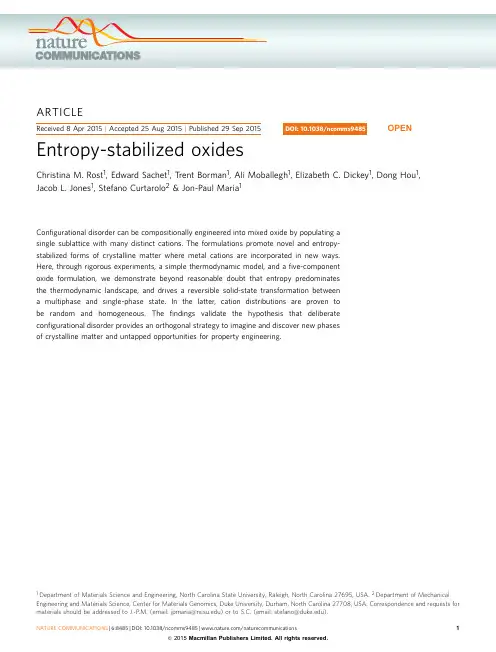
ARTICLEOPENReceived8Apr2015|Accepted25Aug2015|Published29Sep2015Entropy-stabilized oxidesChristina M.Rost1,Edward Sachet1,Trent Borman1,Ali Moballegh1,Elizabeth C.Dickey1,Dong Hou1,Jacob L.Jones1,Stefano Curtarolo2&Jon-Paul Maria1Conﬁgurational disorder can be compositionally engineered into mixed oxide by populating asingle sublattice with many distinct cations.The formulations promote novel and entropy-stabilized forms of crystalline matter where metal cations are incorporated in new ways.Here,through rigorous experiments,a simple thermodynamic model,and aﬁve-componentoxide formulation,we demonstrate beyond reasonable doubt that entropy predominatesthe thermodynamic landscape,and drives a reversible solid-state transformation betweena multiphase and single-phase state.In the latter,cation distributions are proven tobe random and homogeneous.Theﬁndings validate the hypothesis that deliberateconﬁgurational disorder provides an orthogonal strategy to imagine and discover new phasesof crystalline matter and untapped opportunities for property engineering.1Department of Materials Science and Engineering,North Carolina State University,Raleigh,North Carolina27695,USA.2Department of Mechanical Engineering and Materials Science,Center for Materials Genomics,Duke University,Durham,North Carolina27708,USA.Correspondence and requests for materials should be addressed to J.-P.M.(email:jpmaria@)or to S.C.(email:stefano@).A grand challenge facing materials science is the continuoushunt for advanced materials with properties that satisfythe demands of rapidly evolving technology needs.The materials research community has been addressing this problem since the early1900s when Goldschmidt reported the‘the method of chemical substitution’1that combined a tabulation of cationic and anionic radii with geometric principles of ion packing and ion radius ratios.Despite its simplicity,this model enabled a surprising capability to predict stable phases and structures.As early as1926many of the technologically important materials that remain subjects of contemporary research were identiﬁed (though their properties were not known);BaTiO3,AlN,GaP, ZnO and GaAs are among that list.These methods are based on overarching natural tendencies for binary,ternary and quaternary structures to minimize polyhedral distortions,maximize spaceﬁlling and adopt polyhedral linkages that preserve electroneutrality1–3.The structure-ﬁeld maps compiled by Muller and Roy catalogue the crystallographic diversity in the context of these largely geometry-based predictions4.There are,however,limitations to the predictive power,particularly when factors like partial covalency and heterodesmic bonding are considered.To further expand the library of advanced materials and property opportunities,our community explores possibilities based on mechanical strain5,artiﬁcial layering6,external ﬁelds7,combinatorial screening8,interface engineering9,10and structuring at the nanoscale6,11.In many of these efforts, computation and experiment are important companions.Most recently,high-throughput methods emerged as a power-ful engine to assess huge sections of composition space12–17and identiﬁed rapidly new Heusler alloys,extensive ion substitution schemes18,19,new18-electron ABX compounds20and new ferroic semiconductors21.While these methods offer tremendous predictive power and an assessment of composition space intractable to experiment, they often utilize density functional theory calculations conducted at0K.Consequently,the predicted stabilities are based on enthalpies of formation.As such,there remains a potential section of discovery space at elevated temperatures where entropy predominates the free-energy landscape.This landscape was explored recently by incorporating deliberatelyﬁve or more elemental species into a single lattice with random occupancy.In such crystals,entropic contributions to the free energy,rather than the cohesive energy, promote thermodynamic stability atﬁnite temperatures.The approach is being explored within the high-entropy-alloy family of materials(HEAs)22,in which extremely attractive properties continue to be found23,24.In HEAs,however,discussion remains regarding the true role of conﬁgurational entropy25–28, as samples often contain second phases,and there are uncertainties regarding short-range order.In response to these open discussions,HEAs have been referred to recently as multiple-principle-element alloys29.It is compelling to consider similar phenomena in non-metallic systems,particularly considering existing information from entropy studies in mixed oxides.In1967Navrotsky and Kleppa showed how conﬁgurational entropy regulates the normal-to-inverse transformation in spinels,where cations transition between ordered and disordered site occupancy among the available sublattices30,31.These fundamental thermodynamic studies lead one to hypothesize that in principle,sufﬁcient temperature would promote an additional transition to a structure containing only one sublattice with random cation occupancy.From experiment we know that before such transitions,normal materials melt,however,it is conceivable that synthetic formulations exist,which exhibit them.Inspired by research activities in the metal alloy communities and fundamental principles of thermodynamics we extend the entropy concept toﬁve-component oxides.With unambiguous experiments we demonstrate the existence of a new class of mixed oxides that not only contains high conﬁgurational entropy but also is indeed truly entropy stabilized.In addition,we present a hypothesis suggesting that entropy stabilization is particularly effective in a compound with ionic character.ResultsChoosing an appropriate experimental candidate.The candi-date system is an equimolar mixture of MgO,CoO,NiO,CuO and ZnO,(which we label as‘E1’)so chosen to provide the appropriate diversity in structures,coordination and cationic radii to test directly the entropic ansatz.The rationale for selection is as fol-lows:the ensemble of binary oxides should not exhibit uniform crystal structure,electronegativity or cation coordination,and there should exist pairs,for example,MgO–ZnO and CuO–NiO, that do not exhibit extensive solubility.Furthermore,the entire collection should be isovalent such that relative cation ratios can be varied continuously with electroneutrality preserved at the net cation to anion ration of unity.Tabulated reference data for each component,including structure and ionic radius,can be found in Supplementary Table1.Testing reversibility.In theﬁrst experiment,ceramic pellets of E1are equilibrated in an air furnace and quenched to room temperature.The temperature spanned a range from700to 1,100°C,in50-°C increments.X-ray diffraction patterns showing the phase evolution are depicted in Fig.1.After700°C,two prominent phases are observed,rocksalt and tenorite.The tenorite phase fraction reduces with increasing equilibration temperature.Full conversion to single-phase rocksalt occurs between850and900°C,after which there are no additional peaks,the background is low andﬂat,and peak widths are narrow in two-theta(2y)space.Reversibility is a requirement of entropy-driven transitions. Consequently,low-temperature equilibration should transform homogeneous1,000°C-equilibrated E1back to its multiphase state(and vice versa on heating).Figure1also shows a sequence of X-ray diffraction patterns for such a thermal excursion;initial equilibration at1,000°C,a second anneal at750°C,andﬁnally a return to1,000°C.The transformation from single phase,to multiphase,to single phase is evident by the X-ray patterns and demonstrates an enantiotropic(that is,reversible with tempera-ture32)phase transition.Testing entropy though composition variation.A composition experiment is conducted to further characterize this phase tran-sition to the random solid solution state.If the driving force is entropy,altering the relative cation ratios will inﬂuence the transition temperature.Any deviation from equimolarity will reduce the number of possible conﬁgurations O(S c¼k B log(O)), thus increasing the transition temperature.Because S c(x i)is logarithmically linked to mole fraction via B x i log(x i),the com-positional dependence is substantial.This dependency underpins our gedankenexperiment where the role of entropy can be tested by measuring the dependency of transition temperature as a function of the total number of components present,and of the composition of a single component about the equimolar formulation.The calculated entropy trends for an ideal mixture are illustrated in Fig.2b,which plots conﬁgurational entropy for a set of mixtures having N species where the composition of an individual species is changed and the others(NÀ1)are keptequimolar.Two dependencies become apparent:the entropy increases as new species are added and the maximum entropy is achieved when all the species have the same fraction.Both dependencies assume ideal random mixing.Two series of composition-varying experiments investigate the existence of these trends in formulation E1.The ﬁrst experiment monitors phase evolution in ﬁve compounds,each related to the parent E1by the extraction of a single component.The sets are equilibrated at 875°C (the threshold temperature for complete solubility)for 12h.The diffraction patterns in Fig.2a show that removing any component oxide results in material with multiple phases.A four-species set equilibrated under these conditions never yields a single-phase material.The second experiment uses ﬁve individual phase diagrams to explore the conﬁgurational entropy versus composition trend.In each,the composition of a single component is varied by ±2,±6and ±10%increments about the equimolar composition while the others are kept even.Since any departure from equimolarity reduces the conﬁgurational entropy,it should increase transition temperatures to single phase,if thattransitionI n t e n s i t y2030405060702 (°)801.81,100N =5No ZnONo MgON =4No CuON =3No NiONo CoON =21,0501,000950T e m p e r a t u r e (°C )T e m p e r a t u r e (°C )T e m p e r a t u r e (°C )T e m p e r a t u r e (°C )T e m p e r a t u r e (°C )S /k B9008501,1001,0501,0009509008501,1001,0501,0009509008501,1001,0501,0009509008501,1001,0501,0009509008500.0X NX NiOX CuOX ZnOX MgoX CoO0.5 1.00.10.20.30.10.20.30.10.20.30.10.20.30.10.20.31.62223112202001111.41.21.00.80.60.40.20.0J14**********Figure 2|Compositional analysis.(a )X-ray diffraction analysis for a composition series where individual components are removed from the parent composition E1and heat treated to the conditions that would otherwise produce full solid solution.Asterisks identify peaks from rocksalt while carrots identify peaks from other crystal structures.(b )Calculated conﬁgurational entropy in an N -component solid solutions as a function of mol%of the N th component,and (c –g )partial phase diagrams showing the transition temperature to single phase as a function of composition (solvus )in the vicinity of the equimolar composition where maximum conﬁgurational entropy is expected.Error bars account for uncertainty between temperature intervals.Each phase diagram varies systematically the concentration of one element.L o g i n t e n s i t y750 °C750 °C800 °C850 °C900 °C1,000 °C2001111,000 °C 2 (°)T (200)T (002)T (110)T (200)T (002)T (110)Figure 1|X-ray diffraction patterns for entropy-stabilized oxide formulation E1.E1consists of an equimolar mixture of MgO,NiO,ZnO,CuO and CoO.The patterns were collected from a single pellet.The pellet was equilibrated for 2h at each temperature in air,then air quenched to room temperature by direct extraction from the furnace.X-ray intensity is plotted on a logarthimic scale and arrows indicate peaks associated with non-rocksalt phases,peaks indexed with (T)and with (RS)correspond to tenorite and rocksalt phases,respectively.The two X-ray patterns for 1,000°C annealed samples are offset in 2y for clarity.is in fact entropy driven.The speciﬁc formulations used are given in Supplementary Table 2.Figure 2c–g are phase diagrams of composition versus transformation temperature for the ﬁve sample sets that varied mole fraction of a single component.The diagrams were produced by equilibrating and quenching individual samples in 25°C intervals between 825and 1,125°C to obtain the T trans -composition solvus .In all cases equimolarity always leads to the lowest transformation temperatures.This is in agreement with entropic promotion,and consistent with the ideal model shown in Fig.2b.One set of raw X-ray patterns used to identify T trans for 10%MgO is given as an example in Supplementary Fig.1.Testing endothermicity .Reversibility and compositionally dependent solvus lines indicate an entropy-driven process.As such,the excursion from polyphase to single phase should be endothermic.An entropy-driven solid–solid transformation is similar to melting,thus requires heat from an external source 33.To test this possibility,the phase transformation in formulation E1can be co-analysed with differential scanning calorimetry and in situ temperature-dependent X-ray diffraction using identical heating rates.The data for both measurements are shown in Fig.3.Figure 3a is a map of diffracted intensity versus diffraction angle (abscissa)as a function of temperature.It covers B 4°of 2y space centred about the 111reﬂection for E1.At a temperature interval between 825and 875°C,there is a distinct transition to single-phase rocksalt structure—all diffraction events in that range collapse into an intense o 1114rocksalt peak.Figure 3b contains the companion calorimetric result where one ﬁnds a pronounced endotherm in the identical temperature window.The endothermic response only occurs when the system adds heat to the sample,uniquely consistent with an entropy-driven transformation 33.We note the small mass loss (B 1.5%)at the endothermic transition.This mass loss results from the conversion of some spinel (an intermediate phase seen by X-ray diffraction)to rocksalt,which requires reduction of 3þto 2þcations and release of oxygen to maintain stoichiometry.To address concerns regarding CuO reduction,Supplementary Fig.2shows a differential scanning calorimetry and thermal gravimetric analysis curve for pure CuO collected under the same conditions.There is no oxygen loss in the vicinity of 875°C.Testing homogeneity .All experimental results shown so far support the entropic stabilization hypothesis.However,all assume that homogeneous cation mixing occurs above the tran-sition temperature.It is conceivable that local composition ﬂuc-tuations produce coherent clustering or phase separation events that are difﬁcult to discern by diffraction using a laboratory sealed tube diffractometer.The solvus lines of Fig.2c–g support random mixing,as the most stable composition is equimolar (a condition only expected for ideal/regular solutions),but it is appropriate to ensure self-consistency with direct measurements.To characterize the cation distributions,extended X-ray absorption ﬁne structure (EXAFS)and scanning transmission electron microscopy with energy dispersive X-ray spectroscopy (STEM EDS)is used to analyse structure and chemistry on the local scale.EXAFS data were collected for Zn,Ni,Cu and Co at the Advanced Photon Source 12-BM-B 34,35.The ﬁtted data are shown in Fig.4,the raw data are given in Supplementary Fig.3.The ﬁtted data for each element provide two conclusions:the cation-to-anion ﬁrst-near-neighbour distances are identical (within experimental error of ±0.01Å)and the local structures for each element to approximately seven near-neighbour distances are similar.Both observations are only consistent with a random cation distribution.As a corroborating measure of local homogeneity,chemical analysis was conducted using a probe-corrected FEI Titan STEM with EDS detection.Thin ﬁlm samples of E1,prepared by pulsed laser deposition,are the most suitable samples to make the assessment.Details of preparation are given in the methods,and X-ray and electron diffraction analysis for the ﬁlm are provided in Supplementary Figs 4and 5.The sample was thinned by mechanical polishing and ion milling.Figure 5shows a collection of images including Fig.5a,the high-angle annular dark-ﬁeld signal (HAADF).In Fig.5b–f,the EDS signals for the K a emission energies of Mg,Co,Ni,Cu and Zn are shown (additional lower magniﬁcation images are included in Supplementary Fig.6).All magniﬁcations reveal chemically and structurally homogeneous material.1,100R 111R 111Mass change (%)510151,000900800700600500400300200DSC –30–20Endo DSC (mW) Exo35.536.537.52θ (°)–10010Mass100T e m p e r a t u r e (°C )T e m p e r a t u r e (°C )Figure 3|Demonstrating endothermicity.(a )In situ X-ray diffraction intensity map as a function of 2y and temperature;and (b )differential scanning calorimetry trace for formulation ‘E1’.Note that the conversion to single phase is accompanied by an endotherm.Both experiments were conducted at a heating rate of 5°C min À1.04k (Å–1)(k )×k 2 (Å–2)2ZnNiCuCo681012Figure 4|Extended X-ray absorption ﬁne structure.EXAFS measured at Advanced Photon Source beamlime 12-BM after energy normalization and ﬁtting.Note that the oscillations for each element occur with similar relative intensity and at similar reciprocal spacing.This suggests a similar local structural and chemical environment for each.X-ray diffraction,EXAFS and STEM–EDS probes are sensitive to 10s of nm,10s of Åand 1Ålength scales,respectively.While any single technique could be misinterpreted to conclude homogenous mixing,the combination of X-ray diffraction,EXAFS and STEM–EDS provide very strong evidence.We note,in particular,the similarity in EXAFS oscillations (both in amplitude and position)out to 12inverse angstroms.This similarly would be lost if local ordering or clustering were present.Consequently,we conclude with certainty that the cations are uniformly dispersed.DiscussionThe set of experimental outcomes show that the transition from multiple-phase to single phase in E1is driven by conﬁgurational entropy.To complete our thermodynamic understanding of this system,it is important to understand and appreciate the enthalpic penalties that establish the transition temperature.In so doing,the data set can be tested for self-consistency,and the present data are brought into the context of prior research on oxide solubility.First,we consider an equation relating the initial and ﬁnal states of the proposed phase transition:MgO ðRS ÞþNiO ðRS ÞþCoO ðRS ÞþCuO ðT ÞþZnO ðW Þ¼Mg ;Ni ;Co ;Cu ;Zn ðÞO ðRS ÞFor MgO,NiO and CoO,the crystal structures of the initial and ﬁnal states are identical.If we assume that solution of each into the E1rocksalt phase is ideal,the enthalpy for mixing is zero.For CuO and ZnO,there must be a structural transition to rocksalt on dissolution from tenorite and wurtzite,respectively.If we again assume (for simplicity)that the solution is ideal,the mixing energy is zero,but there is an enthalpic penalty associated with the structure transition.From Davies et al.and Bularzik et al.,we know the reference chemical potential changes for the wurtzite-to-rocksalt and the tenorite-to-rocksalt transitions of ZnO and CuO;they are 25and 22kJ mol À1,respectively 36,37.If we make the assumption that the transition enthalpies of ZnO(wurtzite)to ZnO(rocksalt E1)and CuO(tenorite)to CuO(rocksalt E1)are comparable,then the enthalpic penalty for solution into E1can be estimated.For ZnO and CuO,the transition to solid solution in a rocksalt structure involves an enthalpy change of (0.2)Á(25kJ mol À1)þ(0.2)Á(22kJ mol À1),a total of þ10kJ mol À1.This calculation is based on the productof the mol fraction of each multiplied by the reference transition enthalpy.This assumption is consistent with the report of Davies et al.who showed that the chemical potential of a particular cation in a particular structure is associated with the molar volume of that structure 36.Since the rocksalt phases of ZnO and CuO have molar volumes comparable to E1,their reference transition enthalpy values are considered suitable proxies.In comparison,the maximum theoretically expected conﬁg-urational entropy difference at 875°C (the temperature were we observe the transition experimentally)between the single species and the random ﬁve-species solid solution is B 15kJ mol À1,5kJ mol À1larger than the calculated enthalpy of transition.It is possible that the origins of this difference are related to mixing energy as the reference energy values for structural transitions to rocksalt do not capture that aspect.While the present phase diagrams that monitor T trans as a function of composition demonstrate rather symmetric behaviour about the temperature minima,it is unlikely that mixing enthalpies are zero for all constituents.Indeed,literature reports show that enthalpies of mixing between the constituent oxides in E1are ﬁnite and of mixed sign,and their magnitudes are on the same order as the 5kJ mol À1difference between our calculated predictions 36.This energy difference may be accounted for by ﬁnite and positive mixing enthalpies.Following this argument,we can achieve a self-consistent appreciation for the entropic driving force and the enthalpic penalties for solution formation in E1by considering enthalpies of the associated structural transitions and expected entropy values for ideal cation mixing.As a ﬁnal test,these predictions can be compared with experiment,speciﬁcally by calculating the magnitude of the endotherm observed by DSC at the transition from multiple-phase to single-phase states.Doing so we ﬁnd a value B 12kJ mol À1(with an uncertainty of ±2kJ mol À1).While we acknowledge the challenge of quantitative calorimetry,we note that this experimental result is intermediate to and in close agreement with the predicted values.Compared with metallic alloys,the pronounced impact of entropy in oxides may be surprising given that on a per-atom basis the total disorder per volume of an oxide seems be lower than in a high-entropy alloy,as the anion sublattice is ordered (apart from point defects).The chemically uniform sublattice is perhaps the key factor that retains cation conﬁgurational entropy.As an illustration,consider a comparison between random metal alloys and random metal oxide alloys.Begin by reviewing the case of a two-component metallic mixture A–B.If the mixture is ideal,the energy of interaction E A–B ¼(E A–A þE B–B )/2,there is no enthalpic preference for bonding,and entropy regulates solution formation.In this scenario,all lattice sites are equivalent and conﬁgurational entropy is maximized.This situation,however,never occurs as no two elements have identical electronegativity and radii values.Figure 6a illustrates a two-component alloy scenario A–B where species B is more electronegative than A.Consequently,the interaction energies E A–A ,E B–B and E A–B will be different.A random mixture of A–B will produce lattice sites with a distribution of ﬁrst near neighbours,that is,species A coordinated to 4-B atoms,2-A and 2-B atoms,etc y Different coordinations will have different energy values and the sites are no longer indistinguishable.Reducing the number of equivalent sites reduces the number of possible conﬁgurations and S .Now consider the same two metallic ions co-populating a cation sublattice,as in Fig.6b.In this case,there is always an intermediate anion separating neighbouring cation lattice sites.Again,in the limiting case where only ﬁrst near neighboursareFigure 5|STEM–EDS analysis of E1.(a )HAADF image.Panels labelled as Zn,Ni,Cu,Mg and Co are intensity maps for the respective characteristic X-rays.The individual EDS maps show uniform spatial distributions for each element and are atomically resolved.considered,every cation lattice site is ‘identical’because each has the same immediate surroundings:the interior of an oxygen octahedron.Differentiation between sites is only apparent when the second near neighbours are considered.From the conﬁgura-tional disorder perspective,if each cation lattice site is identical,and thus energetically similar to all others,the number of microstates possible within the macrostate will approach the maximum value.This crystallographic argument is based on the limiting case where ﬁrst-near-neighbour interactions predominate the energy landscape,which is an imperfect approximation.Second and third near neighbours will inﬂuence the distribution of lattice site energies and the number of equivalent microstates—but the impact will be the same in both scenarios.A larger number of equivalent sites in a crystal with an intermediate sublattice will increase S and expand the elemental diversity containable in a single solid solution and to lower the temperature at which the transition to entropic stabilization occurs.We acknowledge the hypothesis nature of this model at this time,and the need for a rigorous theoretical exploration.It is presented currently as a possibility and suggestion for future consideration and testing.We demonstrate that conﬁgurational disorder can promote reversible transformations between a poly-phase mixture and a homogeneous solid solution of ﬁve binary oxides,which do not form solid solutions when any of the constituents are removed provided the same thermal budget.The outcome is representative of a new class of materials called ‘entropy-stabilized oxides’.While entropic effects are known for oxide systems,for example,random cation occupancy in spinels 30,order–disorder transfor-mations in feldspar 38,and oxygen nonstoichiometry in layered perovskites 39,the capacity to actively engineer conﬁgurational entropy by composition,to stabilize a quinternary oxide with a single cation sublattice,and to stabilize unusual cation coordination values is new.Furthermore,these systems provide a unique opportunity to explore the thermodynamics and structure–property relationships in systems with extreme conﬁgurational disorder.Experimental efforts exploring this composition space are important considering that such compounds will be challenging to characterize with computational approaches minimizing formation energy (for example,genetic algorithms)or with adhoc thermodynamic models (for example,CALPHAD,cluster expansion)6.We expect entropic stabilization in systems where near-neighbour cations are interrupted by a common intermediateanion (or vice versa),which includes broad classes of chalcogenides,nitrides and halides;particularly when covalent character is modest.The entropic driving force—engineered by cation composition—provides a departure from traditional crystal-chemical principles that elegantly predict structural trends in the major ternary and quaternary systems.A companion set of structure–property relationships that predict new entropy-stabilized structures with novel cation incorporation await discovery and exploitation.MethodsSolid-state synthesis of bulk materials .MgO (Alfa Aesar,99.99%),NiO (Sigma Aldrich,99%),CuO (Alfa Aesar,99.9%),CoO (Alfa Aesar,99%)and ZnO (Alfa Aesar 99.9%)are massed and combined using a shaker mill and 3-mm diameter yttrium-stabilized zirconia milling media.To ensure adequate mixing,all batches are milled for at least 2h.Mixed powders are then separated into 0.500-g samples and pressed into 1.27-cm diameter pellets using a uniaxial hydraulic press at 31,000N.The pellets are ﬁred in air using a Protherm PC442tube furnace.Temperature evolution of phases .Ceramic pellets of E1are equilibrated in an air furnace and quenched to room temperature by direct extraction from the hot zone.Phase analysis is monitored by X-ray diffraction using a PANalytical Empyrean X-ray diffractometer with Bragg-Brentano optics including programmable diver-gence and receiving slits to ensure constant illumination area,a Ni ﬁlter,and a 1-D 128element strip detector.The equivalent counting time for a conventional point detector would be 30s per point at 0.01°2y increments.Note that all X-ray are collected using substantial counting times and are plotted on a logarithmic scale.To the extent knowable using a laboratory diffractometer,the high-temperature samples are homogeneous and single phase:there are no additional minor peaks,the background is low and ﬂat,and peak widths are sharp in two-theta (2y )space.Temperature-dependent diffraction data are collected with PANalytical Empyrean X-ray diffractometer with Bragg-Brentano optics includingprogrammable divergence and receiving slits to ensure constant illumination area,a Ni ﬁlter,and a 1-D 256element strip detector.The samples are placed in a resistively heated HTK-1200N hot stage in air.The samples are ramped at a constant rate of 5°C min À1with a theta–two theta pattern captured every 1.5min.Calorimetry data are collected using a Netzsch STA 449F1Jupiter system in a Pt crucible at 5°C min À1in ﬂowing air.Determining solvus lines .Five series of powders are mixed where the amount of one constituent oxide is varied from the parent mixture E1.Supplementary Table 2lists the full set of samples synthesized for this experiment.Each individual sample is cycled through a heat-soak-quench sequence at 25°C increments from 850°C up to 1,150°C.The soak time for each cycle is 2h,and samples are then quenched to room temperature in o 1min.After the quenching step for each cycle,samples are immediately analysed for phase identiﬁcation using a PANalytical Empyrean X-ray diffractometer using the conditions identiﬁed above.If more than one phase is present,the sample would be put through the next temperature cycle.The temperature at which the structure is determined to be pure rocksalt,with no discernable evidence of peak splitting or secondary phases,is deemed the transition temperature as a function of composition.Supplementary Fig.1shows an example of the collected X-raypatterns after each cycle using the E1L series with þ10%MgO.Once single phase is achieved,the sample is removed from the sequence.Note that this entire experiment is conducted two times.Initially in 50°C increments and longer anneals,and to ensure accuracy of temperature values and reproducibility,a second time using shorter increments and 25°C anneals.Findings in both sets are identical to within experimental error bar values.In the latter case,error bars correspond to the annealing interval value of 25°C.In the main text relating to Fig.2a we note that in addition to small peaks from second phases,X-ray spectra for N ¼4samples with either NiO or MgO removed show anisotropic peak broadening in 2y and skewed relative intensities where I (200)/I (111)is less than unity.This ratio is not possible for the rocksalt structure.Supplementary Table 3shows the result of calculations of structure factors for a random equimolar rocksalt oxide with composition E1.Calculations show that the 200reﬂection is the strongest,and that the experimentally measured relative intensities of 111/200are consistent with calculations.We use this information as a means too best assess when the transition to single phase occurs since the most likely reason for the skewed relative intensity is an incomplete conversion to the single-phase state.This dependency is highlighted in Supplementary Fig.1.X-ray absorption ﬁne structure .X-ray absorption ﬁne structure (XAFS)is made possible through the general user programme at the Advanced Photon Source in Lemont,IL (GUP-38672).This technique provides a unique way to probe the local environment of a speciﬁc element based on the interference between an emitted core electron and the backscattering from surrounding species.XAFS makes no assumption of structure symmetry or elemental periodicity,making it an ideal means to study disordered materials.During the absorption process,coreelectronsBFigure 6|Binary metallic compared with a ternary oxide.A schematic representation of two lattices illustrating how the ﬁrst-near-neighbour environments between species having different electronegativity (the darker the more negative charge localized)for (a )a random binary metal alloy and (b )a random pseudo-binary mixed oxide.In the latter,near-neighbour cations are interrupted by intermediate common anions.。

非富勒烯受体有机光伏体系的激发态动力学

非富勒烯受体有机光伏体系的激发态动力学
张圣兵;张春峰
【期刊名称】《物理学进展》
【年(卷),期】2022(42)1
【摘要】受益于非富勒烯受体的不断发展,近年来有机光伏器件的性能得到长足进步。

传统富勒烯受体有机光伏体系下建立起来的电荷拆分和能量损耗模型,不完全
适用于非富勒烯受体体系。

我们利用超快光谱学方法,发现在模型体系中,非富勒烯
受体畴内非局域激发态代替界面电荷转移态介导了电荷拆分的空穴转移通道,在很
小的驱动能下实现高效电荷拆分。

非富勒烯体系中双分子复合过程在能量损耗中扮演重要角色,分子氟化设计可以改变能级排列,抑制双分子复合产生的三线态,从而抑制损耗。

分子间相互作用调控关键能级位置,可用以调控非富勒烯光伏体系光电流
产生机制,有效抑制损耗通道,进一步提升有机光伏体系的效率。

【总页数】7页(P27-33)
【作者】张圣兵;张春峰
【作者单位】江苏省通州高级中学;南京大学物理学院
【正文语种】中文
【中图分类】TQ317;TM914.4
【相关文献】
1.光电转换率超过12%的含氯非富勒烯受体基有机光伏器件
2.光电转换率超过12％的含氯非富勒烯受体基有机光伏器件
3.苯环侧链喹喔啉非富勒烯受体的合成及光
伏性能4.GW/BSE级别下的非绝热动力学模拟揭示桥连化学键对调控酞菁锌-富勒烯给体-受体复合物激发态弛豫过程的重要作用5.非富勒烯有机光伏体系三线态损耗通道的分子氟化调控
因版权原因，仅展示原文概要，查看原文内容请购买。

基于maxent_模型的迎春樱桃潜在适生区预测

第４７卷㊀第４期２０２３年７月南京林业大学学报（自然科学版）ＪｏｕｒｎａｌｏｆＮａｎｊｉｎｇＦｏｒｅｓｔｒｙＵｎｉｖｅｒｓｉｔｙ（ＮａｔｕｒａｌＳｃｉｅｎｃｅｓＥｄｉｔｉｏｎ）Ｖｏｌ．４７，Ｎｏ．４Ｊｕｌ．，２０２３㊀收稿日期Ｒｅｃｅｉｖｅｄ：２０２１⁃０８⁃０９㊀㊀㊀㊀修回日期Ａｃｃｅｐｔｅｄ：２０２２⁃０２⁃０６㊀基金项目：江苏省重点研发计划（现代农业）面上项目（ＥＢ２０２０３４３）；徐州市科技项目（ＫＣ２１３３６）㊂㊀第一作者：杨宏（１６２２８５１６４８＠ｑｑ．ｃｏｍ）㊂∗通信作者：伊贤贵（ｙｉｘｉａｎｇｕｉ＠ｎｊｆｕ．ｅｄｕ．ｃｎ），副教授，博士㊂㊀引文格式：杨宏，董京京，吴桐，等．基于ＭａｘＥｎｔ模型的迎春樱桃潜在适生区预测［Ｊ］．南京林业大学学报（自然科学版），２０２３，４７（４）：１３１－１３８．ＹＡＮＧＨ，ＤＯＮＧＪＪ，ＷＵＴ，ｅｔａｌ．ＰｒｅｄｉｃｔｉｏｎｏｆｐｏｔｅｎｔｉａｌｓｕｉｔａｂｌｅａｒｅａｓｏｆＣｅｒａｓｕｓｄｉｓｃｏｉｄｅａｉｎＣｈｉｎａｂａｓｅｄｏｎｔｈｅＭａｘＥｎｔｍｏｄｅｌ［Ｊ］．ＪｏｕｒｎａｌｏｆＮａｎｊｉｎｇＦｏｒｅｓｔｒｙＵｎｉｖｅｒｓｉｔｙ（ＮａｔｕｒａｌＳｃｉｅｎｃｅｓＥｄｉｔｉｏｎ），２０２３，４７（４）：１３１－１３８．ＤＯＩ：１０．１２３０２／ｊ．ｉｓｓｎ．１０００－２００６．２０２１０８０１４．基于ＭａｘＥｎｔ模型的迎春樱桃潜在适生区预测杨㊀宏，董京京，吴㊀桐，周华近，陈㊀洁，李㊀蒙，王贤荣，伊贤贵∗（南京林业大学，南方现代林业协同创新中心，南京林业大学生态与环境学院，南京林业大学樱花研究中心，江苏㊀南京㊀２１００３７）摘要：ʌ目的ɔ基于迎春樱桃（Ｃｅｒａｓｕｓｄｉｓｃｏｉｄｅａ）在当代（１９７０２０００年）及未来（２０５０ｓ，２０７０ｓ）气候变化下（ＲＣＰ２．６㊁ＲＣＰ４．５㊁ＲＣＰ８．５）适生区的面积变化研究，预测其潜在适生区为迎春樱桃的种质资源保护与利用提供参考依据㊂ʌ方法ɔ基于１９个气候变量和３个地形因子，结合迎春樱桃现有的５２条有效标本记录信息，利用最大熵ＭａｘＥｎｔ模型并结合地理信息系统软件（Ａｒｃ⁃ＧＩＳ），分析影响迎春樱桃分布的主要因素，预测迎春樱桃的潜在分布区㊂ʌ结果ɔ当前环境条件下迎春樱桃潜在适生区主要分布于长江中下游地区，影响物种分布的主要气候因子是最干季降水量（ｂｉｏ１７）㊁最冷月最低温（ｂｉｏ６）㊁季节性温度变化（ｂｉｏ４）和地形因子坡度（ｓｌｏ）㊂在未来气候（ＢＣＣ⁃ＣＳＭ１．１）条件下其适生区总面积呈减少趋势，但是在２０５０ｓ时期，温室气体中等浓度的排放条件下（ＲＣＰ４．５），物种总适生区面积出现最大值，为７．４９ˑ１０５ｋｍ２；而２０５０ｓ和２０７０ｓ时期低浓度（ＲＣＰ２．６）和中等浓度（ＲＣＰ４．５）温室气体的排放条件下，物种的中度适生区面积保持不变㊂ʌ结论ɔ迎春樱桃适生分布区主要分布于长江中下游地区，江西㊁安徽㊁湖北㊁江苏与浙江等低山地区为迎春樱桃种质资源分布的核心区域㊂关键词：迎春樱桃；适生区；ＭａｘＥｎｔ模型；种质资源中图分类号：Ｓ７１８㊀㊀㊀㊀㊀㊀㊀文献标志码：Ａ开放科学（资源服务）标识码（ＯＳＩＤ）：文章编号：１０００－２００６（２０２３）０４－０１３１－０８ＰｒｅｄｉｃｔｉｏｎｏｆｐｏｔｅｎｔｉａｌｓｕｉｔａｂｌｅａｒｅａｓｏｆＣｅｒａｓｕｓｄｉｓｃｏｉｄｅａｉｎＣｈｉｎａｂａｓｅｄｏｎｔｈｅＭａｘＥｎｔｍｏｄｅｌＹＡＮＧＨｏｎｇ，ＤＯＮＧＪｉｎｇｊｉｎｇ，ＷＵＴｏｎｇ，ＺＨＯＵＨｕａｊｉｎ，ＣＨＥＮＪｉｅ，ＬＩＭｅｎｇ，ＷＡＮＧＸｉａｎｒｏｎｇ，ＹＩＸｉａｎｇｕｉ∗（Ｃｏ⁃ＩｎｎｏｖａｔｉｏｎＣｅｎｔｅｒｆｏｒＳｕｓｔａｉｎａｂｌｅＦｏｒｅｓｔｒｙｉｎＳｏｕｔｈｅｒｎＣｈｉｎａ，ＣｏｌｌｅｇｅｏｆＢｉｏｌｏｇｙａｎｄｔｈｅＥｎｖｉｒｏｎｍｅｎｔ，ＣｅｒａｓｕｓＲｅｓｅａｒｃｈＣｅｎｔｅｒ，ＮａｎｊｉｎｇＦｏｒｅｓｔｒｙＵｎｉｖｅｒｓｉｔｙ，Ｎａｎｊｉｎｇ２１００３７，Ｃｈｉｎａ）Ａｂｓｔｒａｃｔ：ʌＯｂｊｅｃｔｉｖｅɔＢａｓｅｄｏｎＣｅｒａｓｕｓｄｉｓｃｏｉｄｅａｏｆｃｏｎｔｅｍｐｏｒａｒｙ（１９７０－２０００）ｓｕｉｔａｂｌｅａｒｅａｓａｎｄｔｈｅａｄａｐｔｉｖｅｒｅｇｉｏｎｏｆｔｈｅｆｕｔｕｒｅ（２０５０ｓ，２０７０ｓ）ｕｎｄｅｒｃｌｉｍａｔｅｃｈａｎｇｅ（ＲＣＰ２．６，ＲＣＰ４．５ａｎｄＲＣＰ８．５），ｔｈｅｓｅｒｅｓｕｌｔｓｐｒｏｖｉｄｅｄａｒｅｆｅｒｅｎｃｅｆｏｒｔｈｅｐｒｏｔｅｃｔｉｏｎａｎｄｕｔｉｌｉｚａｔｉｏｎｏｆＣ．ｄｉｓｃｏｉｄｅａｇｅｒｍｐｌａｓｍｒｅｓｏｕｒｃｅｓ．ʌＭｅｔｈｏｄɔＢａｓｅｄｏｎ１９ｃｌｉｍａｔｅｖａｒｉａｂｌｅｓａｎｄｔｈｒｅｅｔｏｐｏｇｒａｐｈｉｃｆａｃｔｏｒｓ，ｃｏｍｂｉｎｅｄｗｉｔｈ５２ｖａｌｉｄｓｐｅｃｉｍｅｎｓ，ｔｈｅｍａｘｉｍｕｍｅｎｔｒｏｐｙ（ＭａｘＥｎｔ）ｍｏｄｅｌａｎｄＡｒｃ⁃ＧＩＳｓｏｆｔｗａｒｅｗｅｒｅｕｓｅｄｔｏａｎａｌｙｚｅａｎｄｐｒｅｄｉｃｔｔｈｅｍａｉｎｆａｃｔｏｒｓａｎｄｔｈｅｉｒｐｏｔｅｎｔｉａｌｄｉｓｔｒｉｂｕｔｉｏｎａｒｅａｓｏｆｔｈｉｓｓｐｅｃｉｅｓ．ʌＲｅｓｕｌｔɔＵｎｄｅｒｃｕｒｒｅｎｔｅｎｖｉｒｏｎｍｅｎｔａｌｃｏｎｄｉｔｉｏｎｓ，ｔｈｅｐｏｔｅｎｔｉａｌｌｙｓｕｉｔａｂｌｅａｒｅａｓｆｏｒＣ．ｄｉｓｃｏｉｄｅａａｒｅｍａｉｎｌｙｄｉｓｔｒｉｂｕｔｅｄｉｎｔｈｅｍｉｄｄｌｅａｎｄｌｏｗｅｒｒｅａｃｈｅｓｏｆｔｈｅＹａｎｇｔｚｅＲｉｖｅｒ．Ｔｈｅｍａｉｎｃｌｉｍａｔｉｃｆａｃｔｏｒｓａｆｆｅｃｔｉｎｇｉｔｓｄｉｓｔｒｉｂｕｔｉｏｎｗｅｒｅｐｒｅｃｉｐｉｔａｔｉｏｎｏｆｔｈｅｄｒｉｅｓｔｑｕａｒｔｅｒ（ｂｉｏ１７），ｍｉｎｉｍｕｍｔｅｍｐｅｒａｔｕｒｅｏｆｔｈｅｃｏｌｄｅｓｔｍｏｎｔｈ（ｂｉｏ６），ｔｅｍｐｅｒａｔｕｒｅｓｅａｓｏｎａｌｉｔｙ（ｂｉｏ４），ａｎｄｓｌｏｐｅ（ｓｌｏ）．Ｉｎｔｈｅｆｕｔｕｒｅｃｌｉｍａｔｅ（ＢＣＣ⁃ＣＳＭ１．１），ｔｈｅｔｏｔａｌｓｕｉｔａｂｌｅａｒｅａｏｆｓｐｅｃｉｅｓｗｉｌｌｄｅｃｒｅａｓｅｄ，ｈｏｗｅｖｅｒ，ｉｎｔｈｅ２０５０ｓ，ｕｎｄｅｒｍｏｄｅｒａｔｅｇｒｅｅｎｈｏｕｓｅｇａｓｅｍｉｓｓｉｏｎｃｏｎｄｉｔｉｏｎｓ（ＲＣＰ４．５），ｔｈｅｔｏｔａｌｓｕｉｔａｂｌｅａｒｅａｏｆｓｐｅｃｉｅｓｗｉｌｌｒｅａｃｈａｍａｘｉｍｕｍｏｆ７．４９ˑ１０５ｋｍ２．Ｈｏｗｅｖｅｒ，ｕｎｄｅｒｔｈｅｃｏｎｄｉｔｉｏｎｓｏｆｌｏｗ（ＲＣＰ２．６）ａｎｄｍｏｄｅｒａｔｅ（ＲＣＰ４．５）ｇｒｅｅｎｈｏｕｓｅｇａｓｅｍｉｓｓｉｏｎｓｉｎｔｈｅ２０５０ｓａｎｄｔｈｅ２０７０ｓ，ｔｈｅｍｏｄｅｒａｔｅｌｙｓｕｉｔａｂｌｅａｒｅａｓｒｅｍａｉｎｅｄｕｎｃｈａｎｇｅｄ．ʌＣｏｎｃｌｕｓｉｏｎɔＴｈｅｓｕｉｔａｂｌｅｄｉｓｔｒｉｂｕｔｉｏｎａｒｅａｏｆＣ．ｄｉｓｃｏｉｄｅａｉｓｍａｉｎｌｙｉｎｔｈｅｍｉｄｄｌｅａｎｄｌｏｗｅｒｒｅａｃｈｅｓｏｆｔｈｅＹａｎｇｔｚｅＲｉｖｅｒ，ａｎｄｔｈｅｌｏｗｍｏｕｎｔａｉｎｏｕｓａｒｅａｓｏｆＪｉａｎｇｘｉ，Ａｎｈｕｉ，Ｈｕｂｅｉ，ＪｉａｎｇｓｕａｎｄＺｈｅｊｉａｎｇＰｒｏｖｉｎｃｅｓａｒｅｔｈｅｃｏｒｅａｒｅａｓｏｆｔｈｉｓｇｅｒｍｐｌａｓｍｒｅｓｏｕｒｃｅｓｄｉｓｔｒｉｂｕｔｉｏｎ．南京林业大学学报（自然科学版）第４７卷Ｋｅｙｗｏｒｄｓ：Ｃｅｒａｓｕｓｄｉｓｃｏｉｄｅａ；ｓｕｉｔａｂｌｅａｒｅａ；ＭａｘＥｎｔｍｏｄｅｌ；ｇｅｒｍｐｌａｓｍｒｅｓｏｕｒｃｅｓ㊀㊀樱花为世界著名观赏花木，隶属于蔷薇科（Ｒｏｓａｃｅａｅ）樱属（Ｃｅｒａｓｕｓ），广泛分布于北半球的温带与亚热带地区㊂我国拥有世界最丰富的樱属种质资源，野生樱花资源约４５种［１］，但极少数被推广利用㊂迎春樱桃（Ｃｅｒａｓｕｓｄｉｓｃｏｉｄｅａ）为我国特有的樱属种质资源，其树形优美，枝条纤细，先花后叶，花粉白色且密集而整齐，花期早，具有极高的观赏价值，是国产樱属资源中最具应用价值的早春观花树种之一㊂迎春樱桃主要分布于安徽㊁浙江㊁江西等省份［２］，喜光且喜温暖湿润的环境，天然分布于海拔２００１１００ｍ的山谷或溪边［３］㊂气候变化对植被［４］㊁生态系统功能［５］㊁生物多样性［６］㊁植物物候节律［７－８］等产生重大影响，了解未来气候变化对物种分布及适生区的潜在变化，对物种保护利用及对策制定具有重要意义㊂近些年来陆续有樱属植物适生区的研究，如：赖铭婕等［９］通过对６种原产我国的野生樱桃（Ｃｅｒａｓｕｓｓｐｐ．）在广东的适生区进行预测和分析，表明年均温是６个种共同的主导气候限制因子；李蒙等［１０］通过对山樱花（Ｃｅｒａｓｕｓｓｅｒｒｕｌａｔａ）地理分布与水热环境的因子关系分析表明，山樱花热量分布范围整体偏低，影响其分布的重要环境因子为年均温㊁纬度㊁极端低温㊁１月均温和海拔；朱弘等［１１］进行了浙闽樱桃（Ｃｅｒａｓｕｓｓｃｈｎｅｉｄｅｒｉａｎａ）地理分布模拟及气候限制因子分析，发现年降水量㊁最湿季节降雨量㊁最暖季降雨量㊁温度季节变化方差等水热条件是影响浙闽樱桃当下适生区的气候限制因子㊂有关迎春樱桃的研究主要集中在形态标记［１２］与遗传多样性分析［１３］等方面，对其在大尺度的潜在适生区及影响因子等研究鲜见报道㊂生态位理论的模型主要是利用已有的物种分布资料和环境数据产生以生态位为基础的物种生态需求［８］，目前常用于生态位研究的模型有ＧＡＲＰ㊁ＭａｘＥｎｔ㊁ＥＮＦＡ㊁Ｂｉｏｃｌｉｍ和Ｄｏｍａｉｎ等５种，相较而言，ＭａｘＥｎｔ模型具有更好的预测精度［１４］㊂在猕猴桃（Ａｃｔｉｎｉｄｉａａｒｇｕｔａ）［１５－１６］㊁金钱松（Ｐｓｅｕｄｏｌａｒｉｘａｍａｂｉｌｉｓ）［１７］㊁桫椤（Ａｌｓｏｐｈｉｌａｓｐｉｎｕ⁃ｌｏｓａ）［１８－１９］㊁青钱柳［２０］㊁珙桐（Ｄａｖｉｄｉａｉｎｖｏｌｕｃｒａ⁃ｔａ）［２１－２２］等中国特有物种的适生区研究中取得良好预测结果，为目标物种的保护与利用提供了科学依据㊂本研究以迎春樱桃的地理分布数据及当代（１９７０２０００年）和未来（２１世纪５０７０年代）气候数据为基础，利用ＭａｘＥｎｔ模型预测当代和未来气候环境下迎春樱桃的潜在分布区，分析影响迎春樱桃分布的主要因素，以期更好地了解迎春樱桃在未来气候变化下的分布范围，为其种质资源的保护与利用提供理论依据㊂１㊀材料与方法１．１㊀数据来源１）标本数据收集㊂为了获得迎春樱桃在我国的地理分布数据，借助中国数字植物标本馆（ｈｔ⁃ｔｐｓ：／／ｗｗｗ．ｃｖｈ．ａｃ．ｃｎ／）查阅公开发表的相关资料，并对迎春樱桃分布点进行统计，对于查阅到的标本只有分布点描述记录而没有经纬度记录时借助ｌｏ⁃ｃａｓｐａｃｅｖｉｅｒ网站（ｈｔｔｐ：／／ｗｗｗ．ｌｏｃａｓｐａｃｅ．ｃｎ／）进行解析并确定经纬度㊂将收集到的数据储存于Ｅｘｃｅｌ表格中，运用ＤＶＩ⁃Ａｒｃ⁃ＧＩＳ进行筛选并剔除重复数据，最终获得５２条分布数据用于模型的构建（分辨率１ｋｍ）㊂２）环境数据的收集㊂研究选择的当代（１９７０２０００年）１９个气候因子数据和３个地形因子数据（海拔㊁坡度㊁坡向），均来自世界气候数据库（ｈｔｔｐｓ：／／ｗｗｗ．ｗｏｒｌｄｃｌｉｍ．ｏｒｇ／）；未来２个时段（２１世纪５０年代和７０年代，简称２０５０ｓ㊁２０７０ｓ）的数据来自政府间气候变化委员会（ＩＰＣＣ）第５次气候评估报告中的ＢＣＣ⁃ＣＳＭ１．１大气环流模型［２３］，以及３种典型浓度途径（ｔｈｅｒｅｐｒｅｓｅｎｔａｔｉｖｅｃｏｎｃｅｎ⁃ｔｒａｔｉｏｎｐａｔｈｗａｙｓ，ＲＣＰ２．６㊁ＲＣＰ４．５和ＲＣＰ８．５），共４套气候模拟数据㊂根据ＩＰＣＣ第５次评估报告中的数据，ＲＣＰ２．６表示在严格减排下将全球气候变化控制在高于工业化之前温度２ħ以内的情景，ＲＣＰ４．５表示温室气体在中等浓度的情况，ＲＣＰ８．５代表温室气体在较高排放的情况㊂上述气候数据空间分辨率均为３０ｓ（分辨率１ｋｍ）㊂地图数据以国家基础地理信息中心（ｈｔｔｐ：／／ｗｗｗ．ｎｇｃｃ．ｃｎ／ｎｇｃｃ／）提供的１ʒ４００万中国行政地图为底图［底图审图号：ＧＳ（２０１９）１８２２］㊂１．２㊀气候数据的处理将迎春樱桃的地理信息在Ｅｘｃｅｌ表格中保存（．ｃｓｖ文件），在世界气候数据库中下载的栅格数据导入Ａｒｃ⁃ＧＩＳ中，利用ＳｐａｔｉａｌＡｎａｌｙｓｔ中的提取分析工具，掩膜提取中国行政区以内的１９个生物数据以及３个地形数据（海拔㊁坡度㊁坡向），将提取好的生物栅格数据转换为ＡＳＣ格式并保存㊂１．３㊀ＭａｘＥｎｔ模型建立将收集好的迎春樱桃地理分布数据㊁１９个气２３１㊀第４期杨㊀宏，等：基于ＭａｘＥｎｔ模型的迎春樱桃潜在适生区预测候因子变量以及３个地形因子数据（表１）导入ＭａｘＥｎｔ模型中，勾选ｃｒｅａｔｒｅｓｐｏｎｓｅｃｕｒｖｅｓ㊁ｄｏｊａｃｋ⁃ｋｎｉｉｆｅｔｏｍｅａｓｕｒｅｖａｒｉａｂｉｅｉｍｐｏｒｔａｎｃｅ㊁ｏｕｔｐｕｔｆｏｒｍａｔ为ｌｏｇｉｓｔｉｃ［２４］，随机选取２５％的分布数据作为检验数据，其他为训练数据［２５］，重复１０次运算以排除随机因素的影响，其余则使用模型的默认数值㊂将模型运算输出结果设为ＡＳＣ，输出即为分布概率㊂以０．５为阈值，删除相关系数大且贡献率小的变量，最终按贡献率选取５个气候因子和１个地形因子（ｂｉｏ１７㊁ｂｉｏ６㊁ｂｉｏ４㊁ｓｌｏ㊁ｂｉｏ１９㊁ｂｉｏ９）用于最终的模型构建㊂将选取的５个气候因子和１个地形因子以及地理分布数据导入ＭａｘＥｎｔ模型中再次运算１０次（其余不变）得到分布概率㊂表１㊀用于ＭａｘＥｎｔ模型构建筛选出的环境因子Ｔａｂｌｅ１㊀ＥｎｖｉｒｏｎｍｅｎｔａｌｆａｃｔｏｒｓｆｉｌｔｅｒｅｄｏｕｔｆｏｒＭａｘＥｎｔｍｏｄｅｌｃｏｎｓｔｒｕｃｔｉｏｎ１．４㊀分布图的制作及模型精度的验证将ＭａｘＥｎｔ输出的ＡＳＣ文件导入Ａｒｃ⁃ＧＩＳ转化为栅格文件后进行重分类，根据Ａｒｃ⁃ＧＩＳ中的自然断点法将迎春樱桃的潜在适生区划为４个等级，依次为非适生区㊁低度适生区㊁中度适生区和高度适生区㊂模型精度验证以软件内建的变量分析㊁响应曲线和刀切法验证模型中变量对迎春樱桃适应性的影响㊂以受试者工作特征（ＲＯＣ）曲线下面积（ＡＵＣ）的数值大小对模型精度做出评价，取值范围为［０，１］［２６］，数值越大模型精度越高，表明模型预测效果越好㊂２㊀结果与分析２．１㊀迎春樱桃当代分布图和标本记录点由ＭａｘＥｎｔ输出的ＲＯＣ曲线（图１）可知，该模型的ＡＵＣ均值为０．９８０，标准差为０．００９６［２７］，预测结果很好，且精度很高，因此此次建模结果适用于迎春樱桃在中国潜在适生区的预测㊂根据ＭａｘＥｎｔ模型预测以及Ａｒｃ⁃ＧＩＳ中自带的自然断点法将适生区划为４个等级，结果见图２㊂由图２可知，迎春樱桃主要分布在华中和华东地图１㊀ＭａｘＥｎｔ模型的ＲＯＣ曲线及ＡＵＣ面积Ｆｉｇ．１㊀ＲＯＣｃｕｒｖｅａｎｄＡＵＣａｒｅａｏｆＭａｘＥｎｔｍｏｄｅｌ区，其中：高度适生区主要分布于浙江北部㊁安徽南部和西部㊁江西北部和湖北东南部等地；中度适生区主要分布于江西西部㊁中部和西南部㊁湖南中部㊁浙江南部与江苏等地区；低度适生区主要分布在湖南北部和西部㊁福建北部㊁江西南部等地㊂在当前气候环境下迎春樱桃的适生区面积占中国陆地面积的７．７％，为７．４ˑ１０５ｋｍ２，其中：高度适生区面积为１．０６ˑ１０５ｋｍ２，占１．１％；中度适生区面积为２．２１ˑ１０５ｋｍ２，占２．３％；低度适生区面积为３３１南京林业大学学报（自然科学版）第４７卷底图审图号：ＧＳ（２０１９）１８２２㊂下同㊂Ｔｈｅｓａｍｅｂｅｌｏｗ．图２㊀迎春樱桃在中国的当代适生区和标本记录点Ｆｉｇ．２㊀ＣｏｎｔｅｍｐｏｒａｒｙｓｕｉｔａｂｌｅｇｒｏｗｉｎｇａｒｅａｓａｎｄｓｐｅｃｉｍｅｎｒｅｃｏｒｄｐｏｉｎｔｓｏｆＣｅｒａｓｕｓｄｉｓｃｏｉｄｅａｉｎＣｈｉｎａ４１３ˑ１０５ｋｍ２，占４．３％㊂但是高度适生区面积占比较小，说明迎春樱桃的生长范围比较狭窄，如果受到人为因素的干扰，其栖息地更容易遭到破坏导致种群数量减少㊂ａ．最干季降水量响应曲线ｐｒｅｃｉｐｉｔａｔｉｏｎｉｎｔｈｅｄｒｉｅｓｔｓｅａｓｏｎｒｅｓｐｏｎｓｅｃｕｒｖｅ；ｂ．最冷月最低温响应曲线ｍｉｎｔｅｍｐｅｒａｔｕｒｅｏｆｔｈｅｃｏｌｄｅｓｔｍｏｎｔｈｒｅｓｐｏｎｓｅｃｕｒｖｅ；ｃ．季节性温度变化响应曲线ｓｅａｓｏｎａｌｃｈａｎｇｅｏｆｔｅｍｐｅｒａｔｕｒｅｒｅｓｐｏｎｓｅｃｕｒｖｅ；ｄ．坡度响应曲线ｓｌｏｐｅｒｅｓｐｏｎｓｅｃｕｒｖｅ㊂图４㊀主要环境因子响应曲线Ｆｉｇ．４㊀Ｒｅｓｐｏｎｓｅｃｕｒｖｅｓｏｆｍａｊｏｒｅｎｖｉｒｏｎｍｅｎｔａｌｆａｃｔｏｒｓ２．２㊀环境因子对迎春樱桃适生区的影响２．２．１㊀环境变量分析刀切法检验结果可以反映不同环境变量对迎春樱桃潜在分布的影响，根据输出的Ｊａｃｋｎｉｆｅ图（图３）横坐标表示每次规范训练的结果，条带数值越大说明环境对其影响越大㊂由图３可知，最干旱季度的降水（ｂｉｏ１７）和最冷季度的降水量（ｂｉｏ１９）两个环境变量对迎春樱桃的适生区分布影响最大也是最重要的㊂说明如果预测中不包含这两个环境变量将对迎春樱桃适生区的预测产生极大的影响㊂此外温度和坡度对迎春樱桃分布的影响较大［２８］，这也说明迎春樱桃适宜生活在降水量丰沛且温暖的地区㊂预测结果与物种分布地点相符㊂图３㊀基于刀切法的环境变量分析Ｆｉｇ．３㊀Ａｎａｌｙｓｉｓｏｆｅｎｖｉｒｏｎｍｅｎｔａｌｖａｒｉａｂｌｅｓｂａｓｅｄｏｎｋｎｉｆｅ⁃ｃｕｔｔｉｎｇｍｅｔｈｏｄ２．２．２㊀环境变量贡献率分析根据ＭａｘＥｎｔ模型预测结果可知，温度㊁降水和坡度都不同程度影响迎春樱桃的适生区分布㊂从贡献率来看ｂｉｏ１７最干季降水贡献率最高达到７３４％，其次为最冷月最低温度（ｂｉｏ６）㊁季节性温度变化（ｂｉｏ４）㊁坡度（ｓｌｏ），其贡献率分别为９４％㊁５７％㊁５３％㊂其中最干季降水（ｂｉｏ１７）和最冷月最低温度（ｂｉｏ６）的合计贡献率超过８０％，说明这两个因子对迎春樱桃的分布范围影响最大，其次为ｂｉｏ４和ｓｌｏ，两者占比超过１０％，且ｂｉｏ４和ｓｌｏ两个环境变量在模型中的贡献率要高于重要性，说明环境因子增加了模型的可信度［２９］㊂２．２．３㊀环境变量响应曲线分析根据迎春樱桃环境变量（ｂｉｏ１７㊁ｂｉｏ６㊁ｂｉｏ４㊁ｓｌｏ）与对应的物种存在概率，可获得迎春樱桃环境变量主要响应曲线（图４），以存在概率＞０．５为适宜范围［３０］，则迎春樱桃适宜生长的最干季降水量在１３０１７０ｍｍ，其中最适宜的降水量为１５０ｍｍ；最冷月最低温在－４２ħ，最适宜的温度为０ħ上下；坡度在３ʎ ２７ʎ，其中４ʎ为最适宜的坡度㊂这也从侧面证实了迎春樱桃适宜生长在温暖㊁降水量适宜的缓坡地上㊂若最冷月温度过低或最干季降水量过少都将不利于迎春樱桃的生长㊂４３１㊀第４期杨㊀宏，等：基于ＭａｘＥｎｔ模型的迎春樱桃潜在适生区预测２．３㊀未来气候条件下迎春樱桃潜在的适生区根据ＭａｘＥｎｔ模型预测结果，在未来气候条件下迎春樱桃的适生区有向高纬度迁移的趋势，其中广东㊁福建的适生区面积呈减少趋势（图５）㊂由图５可知，未来迎春樱桃适生区面积总体上呈减少的态势，但是在２０５０ｓ⁃ＲＣＰ４５时总适生区面积达到最大值为７．４９ˑ１０５ｋｍ２，且高度适生区面积有所增加；而在ＲＣＰ２．６（低浓度）和ＲＣＰ４．５（中等浓度）温室气体排放条件下，迎春樱桃的中度适生区面积增加，但在（ＲＣＰ８．５）高浓度温室气体排放条件下中度适生区面积减少；同时在未来气候条件下低度适生区的总体面积也呈减少趋势（表２）㊂图５㊀迎春樱桃未来在中国的适生区Ｆｉｇ．５㊀ＴｈｅｆｕｔｕｒｅｓｕｉｔａｂｌｅｇｒｏｗｉｎｇａｒｅａｏｆＣ．ｄｉｓｃｏｉｄｅａｉｎＣｈｉｎａ表２㊀未来气候条件下迎春樱桃的潜在适生区面积及占当代适生区面积的比例Ｔａｂｌｅ２㊀ＴｈｅｐｏｔｅｎｔｉａｌｓｕｉｔａｂｌｅａｒｅａｏｆＣ．ｄｉｓｃｏｉｄｅａｉｎｔｈｅｆｕｔｕｒｅｃｌｉｍａｔｅａｎｄｉｔｓｐｒｏｐｏｒｔｉｏｎｔｏｔｈｅａｒｅａｏｆｃｏｎｔｅｍｐｏｒａｒｙｓｕｉｔａｂｌｅａｒｅａ情景及年代ｓｃｅｎａｒｉｏａｎｄｅｒａ总适生区ｔｏｔａｌｓｕｉｔａｂｌｅａｒｅａ高度适生区ｈｉｇｈｌｙｓｕｉｔａｂｌｅａｒｅａ中度适生区ｍｏｄｅｒａｔｅｓｕｉｔａｂｌｅａｒｅａ低度适生区ｌｏｗｓｕｉｔａｂｌｅａｒｅａ面积／ˑ１０５ｋｍ２ａｒｅａ占比／％ｐｅｒｃｅｎｔａｇｅ面积／ˑ１０５ｋｍ２ａｒｅａ占比／％ｐｅｒｃｅｎｔａｇｅ面积／ˑ１０５ｋｍ２ａｒｅａ占比／％ｐｅｒｃｅｎｔａｇｅ面积／ˑ１０５ｋｍ２ａｒｅａ占比／％ｐｅｒｃｅｎｔａｇｅ当代ｃｕｒｒｅｎｔ７．４０１．０６２．２１４．１３ＲＣＰ２．６２０５０ｓ７．０１９４．７３１．２５１１７．９２２．４０１０８．６０３．３６８１．３６２０７０ｓ７．２０９７．３０１．０６１００．００２．４０１０８．６０３．７４９０．５６ＲＣＰ４．５２０５０ｓ７．４９１０１．２２１．５４１４５．２８２．４０１０８．６０３．５５８５．６０２０７０ｓ７．３０９８．６５１．２５１１７．９２２．４０１０８．６０３．６５８８．３８ＲＣＰ８．５２０５０ｓ６．９１９３．３８１．２５１１７．９２２．１１９５．４８３．５５８５．６０２０７０ｓ６．９１９３．３８１．３４１２６．４２２．０２９１．４０３．５５８５．６０㊀㊀根据预测结果可知，迎春樱桃的总适生面积变化趋势主要取决于低度适生区面积的变化㊂在２０５０ｓ２０７０ｓ时期的高强度温室气体排放条件下（ＲＣＰ８．５），迎春樱桃总适生区面积出现最小值为６．９１ˑ１０５ｋｍ２，占当代适生区面积的９３．３８％，而在（ＲＣＰ４．５）中等浓度温室气体排放条件下，２０５０ｓ时５３１南京林业大学学报（自然科学版）第４７卷期物种高度适生区面积达到最大值１．５４ˑ１０５ｋｍ２，为当代适生区面积的１４５．２８％；在低等浓度（ＲＣＰ２．６）和中等浓度温室气体排放条件下（ＲＣＰ４．５），同一时期物种的中度适生区面积都保持不变，为２．４０ˑ１０５ｋｍ２，占当代适生区面积的１０８６０％；在低等浓度温室气体排放条件下（ＲＣＰ２６）２０５０ｓ时期的低度适生区面积出现最小值，为３３６ˑ１０５ｋｍ２，占当代低度适生区面积的８１３６％㊂这也说明随着全球气候变暖，水热条件发生改变，使得一些地区不再适宜迎春樱桃的生长，适生区缩小，物种生存压力和种间竞争力加大，物种有趋向濒危的风险㊂３㊀讨㊀论迎春樱桃潜在适生区和高度适生区分别占全国陆地面积的７．７％和１．１％，主要分布于安徽㊁江苏㊁浙江和江西４省，且最干季降水量对迎春樱桃的潜在分布影响最大，其次为温度，该物种能忍受的最冷月温度为－４２ħ，低于－４ħ时不能正常生长㊂环境因子中，坡度对其影响较大，结合野外调查情况，表明此物种适宜生长在光照良好的低山丘陵山地㊂基于ＭａｘＥｎｔ模型，结合气候㊁地理因子与迎春樱桃分布数据计算其适生区面积，通过交叉验证等得出迎春樱桃的适生区主要集中于华中和华东地区，其中高度适生区主要分布于浙江北部㊁安徽南部和西部㊁江西北部和湖北东南部等地；中度适生区主要分布于江西西部㊁中部和西南部㊁湖南中部㊁浙江南部等地区；低度适生区主要分布在湖南北部和西部㊁福建北部㊁江西南部等地㊂当代适生区的分析与南程慧等［３１］㊁商韬等［１３］所记录的分布范围高度吻合，并与‘中国植物志“［２］关于这一物种分布地点的描述一致㊂武夷山地区樱属植物资源丰富，但在长期调查中未发现有迎春樱桃的分布，推测原因与武夷山低度适生区模拟结果及其小乔木树型的性状相关，在发育良好的常绿阔叶林地带性植被中该物种无竞争优势㊂‘中国植物志“［２］与‘江苏植物志“［３２］都未记录迎春樱桃在江苏地区的分布，但实地调查发现，在江苏南部的宜溧山区（１１９ʎ４１ᶄ３５．１２ᵡＥ，３１ʎ１３ᶄ０５．４２ᵡＮ；１１９ʎ３１ᶄ０２．９７ᵡＥ，３１ʎ１０ᶄ１９．０７ᵡＮ）及江苏北部的云台山地区（１１９ʎ２６ᶄ３６．３０ᵡＥ，３４ʎ４２ᶄ４９．８０ᵡＮ）有分布，这与江苏南部宜溧山区为迎春樱桃中度适生区模拟结果一致㊂湖北和湖南地区有着众多的野生樱属资源，但‘湖北植物志“［３３］中没有迎春樱桃分布的记录，推测可能在之前的调查中因交通不便或高山阻隔导致其未被发现㊂根据前人对迎春樱桃系统发育的研究［３４－３６］表明，其与尾叶樱桃㊁山樱花和浙闽樱桃具有较近的遗传关系，同时这些类群地理分布相似，均广泛分布于华中㊁华东一带㊂通过对山樱花㊁浙闽樱桃和尾叶樱桃的适生区研究发现，影响它们分布范围的限制条件为水热条件，这与本研究结果相一致㊂前人对尾叶樱桃的适生区模拟分析［３７－３８］发现其有向东扩展的趋势，而本研究显示迎春樱桃的适生区有向高纬度扩张的趋势，表明樱属植物对水分和热量条件的要求较宽泛；笔者推测迎春樱桃对江苏北部等暖温带地区的次生落叶阔叶林具有较强的竞争优势与适应性，这也是迎春樱桃未来高度适生区朝东北方向扩张的主要原因㊂本研究中选取了３个地形因子结合１９个气候因子数据，发现地形因子也是影响樱属植物的重要因素之一㊂安徽㊁江苏㊁浙江和江西位于中国东部季风区及长江中下游地区，迎春樱桃主要分布于该区的低山丘陵山地，良好的水热条件以及低山环境为迎春樱桃提供了良好的生存环境，模拟结果显示，该区域也是未来气候条件下迎春樱桃的高度适生区㊂在此次模拟中西藏部分地区出现了迎春樱桃的潜在适生区，而查阅当前资料和野外调查暂未发现该地区有天然分布，推测山脉的阻隔以及传播路径过长影响了迎春樱桃在此区域的群体扩张㊂近年来，ＭａｘＥｎｔ模型广泛应用于物种分布方面的预测，本研究利用该模型较好地预测了迎春樱桃在中国的潜在分布区，分析了未来气候条件下迎春樱桃适生区面积的变化趋势㊂迎春樱桃适生区面积总体呈减少趋势，而人为干扰与生境破碎化等问题导致迎春樱桃种群更新与扩张困难㊂随着全球温室效应的加剧以及树种所处生存群落的不断发育，迎春樱桃在群落中将丧失竞争优势，种群数量将不断减少并极易导致其退出现有分布区，未来应注重其种质资源收集㊁引种繁殖及推广利用等方面的研究㊂参考文献（ｒｅｆｅｒｅｎｃｅ）：［１］陈涛，胡国平，王燕，等．我国野生樱属植物种质资源调查㊁收集与保护［Ｊ］．植物遗传资源学报，２０２０，２１（３）：５３２－５４１．ＣＨＥＮＴ，ＨＵＧＰ，ＷＡＮＧＹ，ｅｔａｌ．Ｓｕｒｖｅｙ，ｃｏｌｌｅｃｔｉｏｎａｎｄｃｏｎｓｅｒ⁃ｖａｔｉｏｎｏｆｗｉｌｄＣｅｒａｓｕｓＭｉｌｌ．ｇｅｒｍｐｌａｓｍｒｅｓｏｕｒｃｅｓｉｎＣｈｉｎａ［Ｊ］．ＪＰｌａｎｔＧｅｎｅｔＲｅｓｏｕｒ，２０２０，２１（３）：５３２－５４１．ＤＯＩ：１０．１３４３０／ｊ．ｃｎｋｉ．ｊｐｇｒ．２０１９０７１６００１．［２］中国科学院中国植物志编辑委员会．中国植物志：第３８卷［Ｍ］．北京：科学出版社，１９８６：５２．ＥｄｉｔｏｒｉａｌＣｏｍｍｉｔｔｅｅｏｆＣｈｉｎｅｓｅＦｌｏｒａ，ＣｈｉｎｅｓｅＡｃａｄｅｍｙｏｆＳｃｉｅｎｃｅｓ．ＦｌｏｒａｏｆＣｈｉｎａ：６３１㊀第４期杨㊀宏，等：基于ＭａｘＥｎｔ模型的迎春樱桃潜在适生区预测Ｖｏｌｕｍｅ３８［Ｍ］．Ｂｅｉｊｉｎｇ：ＳｃｉｅｎｃｅＰｒｅｓｓ，１９８６：５２．［３］严春风，徐梁，赵绮，等．我国原生樱属植物资源的分类研究［Ｊ］．江苏林业科技，２０１７，４４（３）：３５－４０．ＹＡＮＣＦ，ＸＵＬ，ＺＨＡＯＱ，ｅｔａｌ．ＣｌａｓｓｉｆｉｃａｔｉｏｎｒｅｓｅａｒｃｈｏｆＣｈｉｎｅｓｅｎａｔｉｖｅＣｅｒａｓｕｓｒｅｓｏｕｒｃｅｓ［Ｊ］．ＪＪｉａｎｇｓｕＦｏｒＳｃｉＴｅｃｈｎｏｌ，２０１７，４４（３）：３５－４０．ＤＯＩ：１０．３９６９／ｊ．ｉｓｓｎ．１００１－７３８０．２０１７．０３．００９．［４］李茂华，都金康，李皖彤，等．１９８２２０１５年全球植被变化及其与温度和降水的关系［Ｊ］．地理科学，２０２０，４０（５）：８２３－８３２．ＬＩＭＨ，ＤＵＪＫ，ＬＩＷＴ，ｅｔａｌ．ＧｌｏｂａｌｖｅｇｅｔａｔｉｏｎｃｈａｎｇｅａｎｄｉｔｓｒｅｌａｔｉｏｎｓｈｉｐｗｉｔｈｐｒｅｃｉｐｉｔａｔｉｏｎａｎｄｔｅｍｐｅｒａｔｕｒｅｂａｓｅｄｏｎＧＬＡＳＳ⁃ＬＡＩｉｎ１９８２－２０１５［Ｊ］．ＳｃｉＧｅｏｇｒＳｉｎ，２０２０，４０（５）：８２３－８３２．ＤＯＩ：１０．１３２４９／ｊ．ｃｎｋｉ．ｓｇｓ．２０２０．０５．０１７．［５］傅伯杰，牛栋，赵士洞．全球变化与陆地生态系统研究：回顾与展望［Ｊ］．地球科学进展，２００５，２０（５）：５５６－５６０．ＦＵＢＪ，ＮＩＵＤ，ＺＨＡＯＳＤ．Ｓｔｕｄｙｏｎｇｌｏｂａｌｃｈａｎｇｅａｎｄｔｅｒｒｅｓｔｒｉａｌｅｃｏｓｙｓｔｅｍｓ：ｈｉｓｔｏｒｙａｎｄｐｒｏｓｐｅｃｔ［Ｊ］．ＡｄｖＥａｒｔｈＳｃｉ，２００５，２０（５）：５５６－５６０．ＤＯＩ：１０．３３２１／ｊ．ｉｓｓｎ：１００１－８１６６．２００５．０５．０１１．［６］何远政，黄文达，赵昕，等．气候变化对植物多样性的影响研究综述［Ｊ］．中国沙漠，２０２１，４１（１）：５９－６６．ＨＥＹＺ，ＨＵＡＮＧＷＤ，ＺＨＡＯＸ，ｅｔａｌ．Ｒｅｖｉｅｗｏｎｔｈｅｉｍｐａｃｔｏｆｃｌｉｍａｔｅｃｈａｎｇｅｏｎｐｌａｎｔｄｉｖｅｒｓｉｔｙ［Ｊ］．ＪＤｅｓｅｒｔＲｅｓ，２０２１，４１（１）：５９－６６．ＤＯＩ：１０．７５２２／ｊ．ｉｓｓｎ．１０００－６９４Ｘ．２０２０．００１０４．［７］付永硕，李昕熹，周轩成，等．全球变化背景下的植物物候模型研究进展与展望［Ｊ］．中国科学：地球科学，２０２０，５０（９）：１２０６－１２１８．ＦＵＹＳ，ＬＩＸＸ，ＺＨＯＵＸＣ，ｅｔａｌ．Ｐｒｏｇｒｅｓｓｉｎｐｌａｎｔｐｈｅｎｏｌｏｇｙｍｏｄｅｌｉｎｇｕｎｄｅｒｇｌｏｂａｌｃｌｉｍａｔｅｃｈａｎｇｅ［Ｊ］．ＳｃｉＳｉｎ（Ｔｅｒｒａｅ），２０２０，５０（９）：１２０６－１２１８．［８］张文秀，寇一翾，张丽，等．采用生态位模拟预测濒危植物白豆杉５个时期的适宜分布区［Ｊ］．生态学杂志，２０２０，３９（２）：６００－６１３．ＺＨＡＮＧＷＸ，ＫＯＵＹＸ，ＺＨＡＮＧＬ，ｅｔａｌ．Ｓｕｉｔａｂｌｅｄｉｓ⁃ｔｒｉｂｕｔｉｏｎｏｆｅｎｄａｎｇｅｒｅｄｓｐｅｃｉｅｓＰｓｅｕｄｏｔａｘｕｓｃｈｉｅｎｉｉ（Ｃｈｅｎｇ）Ｃｈｅｎｇ（Ｔａｘａｃｅａｅ）ｉｎｆｉｖｅｐｅｒｉｏｄｓｕｓｉｎｇｎｉｃｈｅｍｏｄｅｌｉｎｇ［Ｊ］．ＣｈｉｎＪＥｃｏｌ，２０２０，３９（２）：６００－６１３．ＤＯＩ：１０．１３２９２／ｊ．１０００－４８９０．２０２００２．０２８．［９］赖铭婕，吴保欢，崔大方．基于ＤＩＶＡ⁃ＧＩＳ的广东适生樱花预测分析［Ｊ］．广东园林，２０２０，４２（４）：３７－４１．ＬＡＩＭＪ，ＷＵＢＨ，ＣＵＩＤＦ．ＰｒｅｄｉｃｔｉｏｎａｎｄａｎａｌｙｓｉｓｏｆｓｕｉｔａｂｌｅＣｅｒａｓｕｓｓｐｐ．ｉｎＧｕａｎｇｄｏｎｇＰｒｏｖｉｎｃｅｂａｓｅｄｏｎＤＩＶＡ⁃ＧＩＳ［Ｊ］．ＧｕａｎｇｄｏｎｇＬａｎｄｓｃＡｒｃｈｉｔ，２０２０，４２（４）：３７－４１．［１０］李蒙，伊贤贵，王华辰，等．山樱花地理分布与水热环境因子的关系［Ｊ］．南京林业大学学报（自然科学版），２０１４，３８（增刊）：７４－８０．ＬＩＭ，ＹＩＸＧ，ＷＡＮＧＨＣ，ｅｔａｌ．ＳｔｕｄｉｅｓｏｎｔｈｅｒｅｌａｔｉｏｎｓｈｉｐｂｅｔｗｅｅｎＣｅｒａｓｕｓｓｅｒｒｕｌａｔａｄｉｓｔｒｉｂｕｔｉｏｎｒｅｇｉｏｎａｎｄｔｈｅｅｎｖｉｒｏｎｍｅｎｔａｌｆａｃｔｏｒｓ［Ｊ］．ＪＮａｎｊｉｎｇＦｏｒＵｎｉｖ（ＮａｔＳｃｉＥｄ），２０１４，３８（Ｓ１）：７４－８０．ＤＯＩ：１０．３９６９／ｊ．ｉｓｓｎ．１０００－２００６．２０１４．Ｓ１．０１６．［１１］朱弘，尤禄祥，李涌福，等．浙闽樱桃地理分布模拟及气候限制因子分析［Ｊ］．热带亚热带植物学报，２０１７，２５（４）：３１５－３２２．ＺＨＵＨ，ＹＯＵＬＸ，ＬＩＹＦ，ｅｔａｌ．Ｍｏｄｅｌｉｎｇｔｈｅｇｅｏｇｒａｐｈｉｃａｌｄｉｓｔｒｉ⁃ｂｕｔｉｏｎｐａｔｔｅｒｎａｎｄｃｌｉｍａｔｉｃｌｉｍｉｔｅｄｆａｃｔｏｒｓｏｆＣｅｒａｓｕｓｓｃｈｎｅｉｄｅｒｉａｎａ［Ｊ］．ＪＴｒｏｐＳｕｂｔｒｏｐＢｏｔ，２０１７，２５（４）：３１５－３２２．ＤＯＩ：１０．１１９２６／ｊｔｓｂ．３７０２．［１２］南程慧．迎春樱居群变异与繁殖生物学研究［Ｄ］．南京：南京林业大学，２０１２．ＮＡＮＣＨ．Ｓｔｕｄｙｏｎｐｏｐｕｌａｔｉｏｎｖａｒｉａｔｉｏｎａｎｄｒｅ⁃ｐｒｏｄｕｃｔｉｖｅｂｉｏｌｏｇｙｏｆＣｅｒａｓｕｓｄｉｓｃｏｉｄｅａＹüｅｔＬｉ［Ｄ］．Ｎａｎｊｉｎｇ：ＮａｎｊｉｎｇＦｏｒｅｓｔｒｙＵｎｉｖｅｒｓｉｔｙ，２０１２．［１３］商韬，王贤荣，南程慧，等．基于ＳＳＲ标记的迎春樱自然居群遗传多样性分析［Ｊ］．甘肃农业大学学报，２０１３，４８（６）：１０４－１０９，１１５．ＳＨＡＮＧＴ，ＷＡＮＧＸＲ，ＮＡＮＣＨ，ｅｔａｌ．ＧｅｎｅｔｉｃｄｉｖｅｒｓｉｔｙｉｎｎａｔｕｒａｌｐｏｐｕｌａｔｉｏｎｓｏｆＣｅｒａｓｕｓｄｉｓｃｏｉｄｅａｂａｓｅｄｏｎＳＳＲｍａｒｋｅｒｓ［Ｊ］．ＪＧａｎｓｕＡｇｒｉｃＵｎｉｖ，２０１３，４８（６）：１０４－１０９，１１５．ＤＯＩ：１０．１３４３２／ｊ．ｃｎｋｉ．ｊｇｓａｕ．２０１３．０６．０２１．［１４］曹向锋，钱国良，胡白石，等．采用生态位模型预测黄顶菊在中国的潜在适生区［Ｊ］．应用生态学报，２０１０，２１（１２）：３０６３－３０６９．ＣＡＯＸＦ，ＱＩＡＮＧＬ，ＨＵＢＳ，ｅｔａｌ．ＰｒｅｄｉｃｔｉｏｎｏｆｐｏｔｅｎｔｉａｌｓｕｉｔａｂｌｅｄｉｓｔｒｉｂｕｔｉｏｎａｒｅａｏｆＦｌａｖｅｒｉａｂｉｄｅｎｔｉｓｉｎＣｈｉｎａｂａｓｅｄｏｎｎｉｃｈｅｍｏｄｅｌｓ［Ｊ］．ＣｈｉｎＪＡｐｐｌＥｃｏｌ，２０１０，２１（１２）：３０６３－３０６９．ＤＯＩ：１０．１３２８７／ｊ．１００１－９３３２．２０１０．０４３１．［１５］张童，黄治昊，彭杨靖，等．基于ＭａｘＥｎｔ模型的软枣猕猴桃在中国潜在适生区预测［Ｊ］．生态学报，２０２０，４０（１４）：４９２１－４９２８．ＺＨＡＮＧＴ，ＨＵＡＮＧＺＨ，ＰＥＮＧＹＪ，ｅｔａｌ．Ｐｒｅｄｉｃｔｉｏｎｏｆｐｏ⁃ｔｅｎｔｉａｌｓｕｉｔａｂｌｅａｒｅａｓｏｆＡｃｔｉｎｉｄｉａａｒｇｕｔａｉｎＣｈｉｎａｂａｓｅｄｏｎＭａｘＥｎｔｍｏｄｅｌ［Ｊ］．ＡｃｔａＥｃｏｌＳｉｎ，２０２０，４０（１４）：４９２１－４９２８．ＤＯＩ：１０．５８４６／ｓｔｘｂ２０１９０９１６１９２１．［１６］王茹琳，王明田，罗家栋，等．基于ＭａｘＥｎｔ模型的美味猕猴桃在中国气候适宜性分析［Ｊ］．云南农业大学学报（自然科学），２０１９，３４（３）：５２２－５３１．ＷＡＮＧＲＬ，ＷＡＮＧＭＴ，ＬＵＯＪＤ，ｅｔａｌ．ＴｈｅａｎａｌｙｓｉｓｏｆｃｌｉｍａｔｅｓｕｉｔａｂｉｌｉｔｙａｎｄｒｅｇｉｏｎａｌｉｚａｔｉｏｎｏｆＡｃｔｉｎｉｄｉａｄｅｌｉｃｉｏｓａｂｙｕｓｉｎｇＭａｘＥｎｔｍｏｄｅｌｉｎＣｈｉｎａ［Ｊ］．ＪＹｕｎｎａｎＡｇｒｉｃＵｎｉｖ（ＮａｔＳｃｉ），２０１９，３４（３）：５２２－５３１．ＤＯＩ：１０．１２１０１／ｊ．ｉｓｓｎ．１００４－３９０Ｘ（ｎ）．２０１７１１０３９．［１７］王国峥，耿其芳，肖孟阳，等．基于４种生态位模型的金钱松潜在适生区预测［Ｊ］．生态学报，２０２０，４０（１７）：６０９６－６１０４．ＷＡＮＧＧＺ，ＧＥＮＧＱＦ，ＸＩＡＯＭＹ，ｅｔａｌ．ＰｒｅｄｉｃｔｉｎｇＰｓｅｕｄｏｌａｒｉｘａｍａｂｉｌｉｓｐｏｔｅｎｔｉａｌｈａｂｉｔａｔｂａｓｅｄｏｎｆｏｕｒｎｉｃｈｅｍｏｄｅｌｓ［Ｊ］．ＡｃｔａＥｃｏｌＳｉｎ，２０２０，４０（１７）：６０９６－６１０４．ＤＯＩ：１０．５８４６／ｓｔｘｂ２０１９０７０２１３９０．［１８］杨启杰，李睿．桫椤的潜在适生区及其变化［Ｊ］．应用生态学报，２０２１，３２（２）：５３８－５４８．ＹＡＮＧＱＪ，ＬＩＲ．Ｐｒｅｄｉｃｔｉｎｇｔｈｅｐｏ⁃ｔｅｎｔｉａｌｓｕｉｔａｂｌｅｈａｂｉｔａｔｓｏｆＡｌｓｏｐｈｉｌａｓｐｉｎｕｌｏｓａａｎｄｔｈｅｉｒｃｈａｎｇｅｓ［Ｊ］．ＣｈｉｎＪＡｐｐｌＥｃｏｌ，２０２１，３２（２）：５３８－５４８．ＤＯＩ：１０．１３２８７／ｊ．１００１－９３３２．２０２１０２．０１５．［１９］许斌，朱文泉，李培先．不同气候条件下桫椤在中国的潜在适生区分布［Ｊ］．生态学报，２０２０，４０（１７）：６１０５－６１１７．ＸＵＢ，ＺＨＵＷＱ，ＬＩＰＸ．ＰｏｔｅｎｔｉａｌｄｉｓｔｒｉｂｕｔｉｏｎｓｏｆＡｌｓｏｐｈｉｌａｓｐｉｎｕｌｏｓａｕｎｄｅｒｄｉｆｆｅｒｅｎｔｃｌｉｍａｔｅｓｉｎＣｈｉｎａ［Ｊ］．ＡｃｔａＥｃｏｌＳｉｎ，２０２０，４０（１７）：６１０５－６１１７．ＤＯＩ：１０．５８４６／ｓｔｘｂ２０１９０７２４１５６５．［２０］刘清亮，李垚，方升佐．基于ＭａｘＥｎｔ模型的青钱柳潜在适宜栽培区预测［Ｊ］．南京林业大学学报（自然科学版），２０１７，４１（４）：２５－２９．ＬＩＵＱＬ，ＬＩＹ，ＦＡＮＧＳＺ．ＭａｘＥｎｄｍｏｄｅｌ⁃ｂａｓｅｄｉｎｄｅｎｔｉｆｉｃａｔｉｏｎｏｆｐｏｔｅｎｔｉａｌＣｙｃｌｏｃａｒｙａｐａｌｉｕｒｕｓｃｕｌｔｉｖａｔｉｏｎｒｅｇｉｏｎｓ［Ｊ］．ＪＮａｎｊｉｎｇＦｏｒｅＵｎｉｖ（ＮａｔＳｃｉＥｄ），２０１７，４１（４）：２５－２９．ＤＯＩ：１０．３９６９／ｊ．ｉｓｓｎ．１０００－２００６．２０１６０８０１０．［２１］王雨生，王召海，邢汉发，等．基于ＭａｘＥｎｔ模型的珙桐在中国潜在适生区预测［Ｊ］．生态学杂志，２０１９，３８（４）：１２３０－１２３７．ＷＡＮＧＹＳ，ＷＡＮＧＺＨ，ＸＩＮＧＨＦ，ｅｔａｌ．ＰｒｅｄｉｃｔｉｏｎｏｆｐｏｔｅｎｔｉａｌｓｕｉｔａｂｌｅｄｉｓｔｒｉｂｕｔｉｏｎｏｆＤａｖｉｄｉａｉｎｖｏｌｕｃｒａｔａＢａｉｌｌｉｎＣｈｉｎａｂａｓｅｄｏｎＭａｘＥｎｔ［Ｊ］．ＣｈｉｎＪＥｃｏｌ，２０１９，３８（４）：１２３０－１２３７．ＤＯＩ：１０．１３２９２／ｊ．１０００－４８９０．２０１９０４．０２４．［２２］陈俪心，和梅香，王彬，等．基于ＭａｘＥｎｔ模型的凉山山系珙桐种群适宜生境分布及其影响因素分析［Ｊ］．四川大学学报（自然科学版），２０１８，５５（４）：８７３－８８０．ＣＨＥＮＬＸ，ＨＥＭＸ，ＷＡＮＧＢ，ｅｔａｌ．Ａｎａｌｙｓｉｓｏｆｓｕｉｔａｂｌｅｈａｂｉｔａｔｄｉｓｔｒｉｂｕｔｉｏｎａｎｄｉｔｓｉｎ⁃ｆｌｕｅｎｃｅｆａｃｔｏｒｓｏｆＤａｖｉｄｉａｉｎｖｏｌｕｃｒａｔａｉｎＬｉａｎｇｓｈａｎＭｏｕｎｔａｉｎｓｂａｓｅｄｏｎＭａｘＥｎｔｍｏｄｅｌ［Ｊ］．ＪＳｉｃｈｕａｎＵｎｉｖ（ＮａｔＳｃｉＥｄ），２０１８，５５（４）：８７３－８８０．ＤＯＩ：１０．３９６９／ｊ．ｉｓｓｎ．０４９０－６７５６．２０１８．０４．０３５．７３１南京林业大学学报（自然科学版）第４７卷［２３］沈永平，王国亚．ＩＰＣＣ第一工作组第五次评估报告对全球气候变化认知的最新科学要点［Ｊ］．冰川冻土，２０１３，３５（５）：１０６８－１０７６．ＳＨＥＮＹＰ，ＷＡＮＧＧＹ．ＫｅｙｆｉｎｄｉｎｇｓａｎｄａｓｓｅｓｓｍｅｎｔｒｅｓｕｌｔｓｏｆＩＰＣＣＷＧＩｆｉｆｔｈａｓｓｅｓｓｍｅｎｔｒｅｐｏｒｔ［Ｊ］．ＪＧｌａｃｉｏｌＧｅｏｃｒｙｏｌ，２０１３，３５（５）：１０６８－１０７６．ＤＯＩ：１０．７５２２／ｊ．ｉｓｓｎ．１０００－０２４０．２０１３．０１２０．［２４］齐国君，陈婷，高燕，等．基于Ｍａｘｅｎｔ的大洋臀纹粉蚧和南洋臀纹粉蚧在中国的适生区分析［Ｊ］．环境昆虫学报，２０１５，３７（２）：２１９－２２３．ＱＩＧＪ，ＣＨＥＮＴ，ＧＡＯＹ，ｅｔａｌ．ＰｏｔｅｎｔｉａｌｇｅｏｇｒａｐｈｉｃｄｉｓｔｒｉｂｕｔｉｏｎｏｆＰｌａｎｏｃｏｃｃｕｓｍｉｎｏｒａｎｄＰ．ｌｉｌａｃｉｎｕｓｉｎＣｈｉｎａｂａｓｅｄｏｎＭａｘＥｎｔ［Ｊ］．ＪＥｎｖｉｒｏｎＥｎｔｏｍｏｌ，２０１５，３７（２）：２１９－２２３．ＤＯＩ：１０．３９６９／ｊ．ｉｓｓｎ．１６７４－０８５８．２０１５．０２．１．［２５］邹天娇，倪畅，郑曦．基于ＭａｘＥｎｔ模型的北京浅山区珍稀植物适生区预测及管理［Ｊ］．中国城市林业，２０２０，１８（４）：１７－２２．ＺＯＵＴＪ，ＮＩＣ，ＺＨＥＮＧＸ．ＰｒｅｄｉｃｔｉｏｎａｎｄｍａｎａｇｅｍｅｎｔｏｆｒａｒｅｐｌａｎｔｓｕｉｔａｂｌｅａｒｅａｉｎｈｉｌｌｙａｒｅａｓｏｆＢｅｉｊｉｎｇｂａｓｅｄｏｎＭａｘＥｎｔｍｏｄｅｌ［Ｊ］．ＪＣｈｉｎＵｒｂａｎＦｏｒ，２０２０，１８（４）：１７－２２．ＤＯＩ：１０．１２１６９／ｚｇｃｓｌｙ．２０１９．０３．２７．０００１．［２６］柳晓燕，李俊生，赵彩云，等．基于ＭａｘＥｎｔ模型和ＡｒｃＧＩＳ预测豚草在中国的潜在适生区［Ｊ］．植物保护学报，２０１６，４３（６）：１０４１－１０４８．ＬＩＵＸＹ，ＬＩＪＳ，ＺＨＡＯＣＹ，ｅｔａｌ．Ｐｒｅｄｉｃｔｉｏｎｏｆｐｏ⁃ｔｅｎｔｉａｌｓｕｉｔａｂｌｅａｒｅａｏｆＡｍｂｒｏｓｉａａｒｔｅｍｉｓｉｉｆｏｌｉａＬ．ｉｎＣｈｉｎａｂａｓｅｄｏｎＭａｘＥｎｔａｎｄＡｒｃＧＩＳ［Ｊ］．ＪＰｌａｎｔＰｒｏｔ，２０１６，４３（６）：１０４１－１０４８．ＤＯＩ：１０．１３８０２／ｊ．ｃｎｋｉ．ｚｗｂｈｘｂ．２０１６．０６．０２３．［２７］孙蓉，刘影．基于ＭａｘＥｎｔ模型的江西省白桂木生境适宜性评价［Ｊ］．南方林业科学，２０２０，４８（２）：２３－２７．ＳＵＮＲ，ＬＩＵＹ．ＨａｂｉｔａｔｓｕｉｔａｂｉｌｉｔｙｅｖａｌｕａｔｉｏｎｏｆＡｒｔｏｃａｒｐｕｓｈｙｐａｒｇｙｒｅｕｓＨａｎｃｅｉｎＪｉａｎｇｘｉＰｒｏｖｉｎｃｅｂａｓｅｄｏｎＭａｘＥｎｔｍｏｄｅｌ［Ｊ］．ＳｏｕｔｈＣｈｉｎａＦｏｒＳｃｉ，２０２０，４８（２）：２３－２７．ＤＯＩ：１０．１６２５９／ｊ．ｃｎｋｉ．３６－１３４２／ｓ．２０２０．０２．００５．［２８］樊信，盘金文，何嵩涛．气候变化背景下基于ＭａｘＥｎｔ模型的刺梨潜在适生区分布预测［Ｊ］．西北植物学报，２０２１，４１（１）：１５９－１６７．ＦＡＮＸ，ＰＡＮＪＷ，ＨＥＳＴ．ＰｒｅｄｉｃｔｉｏｎｏｆｔｈｅｐｏｔｅｎｔｉａｌｄｉｓｔｒｉｂｕｔｉｏｎｏｆＲｏｓａｒｏｘｂｕｒｇｈｉｉｕｎｄｅｒｔｈｅｂａｃｋｇｒｏｕｎｄｏｆｃｌｉｍａｔｅｃｈａｎｇｅｂａｓｅｄｏｎＭａｘＥｎｔｍｏｄｅｌ［Ｊ］．ＡｃｔａＢｏｔＢｏｒｅａｌｉＯｃｃｉｄｅｎｔａｌｉａＳｉｎ，２０２１，４１（１）：１５９－１６７．ＤＯＩ：１０．７６０６／ｊ．ｉｓｓｎ．１０００－４０２５．２０２１．０１．０１５９．［２９］姚祺，李佶芸，赵垦田．基于ＭａｘＥｎｔ模型的巨柏青藏高原生态适宜性研究［Ｊ］．高原农业，２０２１，５（２）：１０９－１１４．ＹＡＯＱ，ＬＩＪＹ，ＺＨＡＯＫＴ．ＲｅｓｅａｒｃｈｏｎｅｃｏｌｏｇｉｃａｌｓｕｉｔａｂｉｌｉｔｙｏｆｇｉａｎｔｃｙｐｒｅｓｓｏｎＱｉｎｇｈａｉ⁃ＴｉｂｅｔＰｌａｔｅａｕｂａｓｅｄｏｎＭａｘＥｎｔｍｏｄｅｌ［Ｊ］．ＪＰｌａｔｅａｕＡｇｒｉｃ，２０２１，５（２）：１０９－１１４．ＤＯＩ：１０．１９７０７／ｊ．ｃｎｋｉ．ｊｐａ．２０２１．０２．００１．［３０］王广，张莹，张娇，等．基于ＭａｘＥｎｔ模型的半夏潜在适宜分布研究［Ｊ］．武汉轻工大学学报，２０１８，３７（６）：３５－４０．ＷＡＮＧＧ，ＺＨＡＮＧＹ，ＺＨＡＮＧＪ，ｅｔａｌ．ＰｏｔｅｎｔｉａｌｄｉｓｔｒｉｂｕｔｉｏｎｏｆＰｉｎｅｌｌｉａｔｅｒｎａｔａｂａｓｅｄｏｎＭａｘＥｎｔｍｏｄｅｌ［Ｊ］．ＪＷｕｈａｎＰｏｌｙｔｅｃｈＵｎｉｖ，２０１８，３７（６）：３５－４０．ＤＯＩ：１０．３９６９／ｊ．ｉｓｓｎ．２０９５－７３８６．２０１８．０６．００５．［３１］南程慧，伊贤贵，王华辰，等．迎春樱群落主要种群生态位研究［Ｊ］．南京林业大学学报（自然科学版），２０１４，３８（增刊）：８９－９２．ＮＡＮＣＨ，ＹＩＸＧ，ＷＡＮＧＨＣ，ｅｔａｌ．ＳｔｕｄｙｏｎｔｈｅｎｉｃｈｅｏｆｔｈｅｍａｉｎｐｏｐｕｌａｉｔｉｏｎｉｎＣｅｒａｓｕｓｄｉｓｃｏｉｄｅａｃｏｍｍｕｎｉｔｙ［Ｊ］．ＪＮａｎｊｉｎｇＦｏｒＵｎｉｖ（ＮａｔＳｃｉＥｄ），２０１４，３８（Ｓ１）：８９－９２．ＤＯＩ：１０．３９６９／ｊ．ｉｓｓｎ．１０００－２００６．２０１４．Ｓ１．０１８．［３２］江苏省植物研究所．江苏植物志：上册［Ｍ］．南京：江苏人民出版社，１９７７．ＪｉａｎｇｓｕＩｎｓｔｉｔｕｔｅｏｆＢｏｔａｎｙ．ＦｌｏｒａｏｆＪｉａｎｇｓｕ：Ｖｏｌｕｍｅ１［Ｍ］．Ｎａｎｊｉｎｇ：ＪｉａｎｇｓｕＰｅｏｐｌｅｓＰｕｂｌｉｓｈｉｎｇＨｏｕｓｅ，１９７７．［３３］傅书遐．湖北植物志［Ｍ］．武汉：湖北科技出版社，２００２．ＦＵＳＸ．ＦｌｏｒａＨｕｂｅｉｅｎｓｉｓ［Ｍ］．Ｗｕｈａｎ：ＨｕｂｅｉＳｃｉｅｎｃｅａｎｄＴｅｃｈｎｏｌｏｇｙＰｒｅｓｓ，２００２．［３４］ＬＩＭ，ＳＯＮＧＹＦ，ＳＹＬＶＥＳＴＥＲＳＰ，ｅｔａｌ．ＣｏｍｐａｒａｔｉｖｅａｎａｌｙｓｉｓｏｆｔｈｅｃｏｍｐｌｅｔｅｐｌａｓｔｉｄｇｅｎｏｍｅｓｉｎＰｒｕｎｕｓｓｕｂｇｅｎｕｓＣｅｒａｓｕｓ（Ｒｏｓａ⁃ｃｅａｅ）：ｍｏｌｅｃｕｌａｒｓｔｒｕｃｔｕｒｅｓａｎｄｐｈｙｌｏｇｅｎｅｔｉｃｒｅｌａｔｉｏｎｓｈｉｐｓ［Ｊ］．ＰＬｏＳＯｎｅ，２０２２，１７（４）：ｅ０２６６５３５．ＤＯＩ：１０．１３７１／ｊｏｕｒｎａｌ．ｐｏｎｅ．０２６６５３５．［３５］ＹＡＮＪＷ，ＬＩＪＨ，ＹＵＬ，ｅｔａｌ．ＣｏｍｐａｒａｔｉｖｅｃｈｌｏｒｏｐｌａｓｔｇｅｎｏｍｅｓｏｆＰｒｕｎｕｓｓｕｂｇｅｎｕｓＣｅｒａｓｕｓ（Ｒｏｓａｃｅａｅ）：ｉｎｓｉｇｈｔｓｉｎｔｏｓｅｑｕｅｎｃｅｖａｒｉａｔｉｏｎｓａｎｄｐｈｙｌｏｇｅｎｅｔｉｃｒｅｌａｔｉｏｎｓｈｉｐｓ［Ｊ］．ＴｒｅｅＧｅｎｅｔＧｅｎｏｍｅｓ，２０２１，１７（６）：５０．ＤＯＩ：１０．１００７／ｓ１１２９５－０２１－０１５３３－８．［３６］朱弘，伊贤贵，朱淑霞，等．基于叶绿体ＤＮＡａｔｐＢ⁃ｒｂｃＬ片段的典型樱亚属部分种的亲缘关系及分类地位探讨［Ｊ］．植物研究，２０１８，３８（６）：８２０－８２７．ＺＨＵＨ，ＹＩＸＧ，ＺＨＵＳＸ，ｅｔａｌ．ＡｎａｌｙｓｉｓｏｎｒｅｌａｔｉｏｎｓｈｉｐａｎｄｔａｘｏｎｏｍｉｃｓｔａｔｕｓｏｆｓｏｍｅｓｐｅｃｉｅｓｉｎＳｕｂｇ．ＣｅｒａｓｕｓＫｏｅｈｎｅｗｉｔｈｃｈｌｏｒｏｐｌａｓｔＤＮＡａｔｐＢ⁃ｒｂｃＬｆｒａｇｍｅｎｔ［Ｊ］．ＢｕｌｌＢｏｔＲｅｓ，２０１８，３８（６）：８２０－８２７．ＤＯＩ：１０．７５２５／ｊ．ｉｓｓｎ．１６７３－５１０２．２０１８．０６．００４．［３７］朱弘．尾叶樱桃（Ｃｅｒａｓｕｓｄｉｅｌｓｉａｎａ）系统分类地位与种群生物地理学研究［Ｄ］．南京：南京林业大学，２０２０．ＺＨＵＨ．ＰｈｙｌｏｇｅｎｅｔｉｃｐｏｓｉｔｉｏｎａｎｄｐｏｐｕｌａｔｉｏｎｂｉｏｇｅｏｇｒａｐｈｙｏｆＣｅｒａｓｕｓｄｉｅｌ⁃ｓｉａｎａ（Ｒｏｓａｃｅａｅ）［Ｄ］．Ｎａｎｊｉｎｇ：ＮａｎｊｉｎｇＦｏｒｅｓｔｒｙＵｎｉｖｅｒｓｉｔｙ，２０２０．［３８］朱弘，伊贤贵，朱淑霞，等．中国亚热带特有植物尾叶樱桃的研究进展［Ｊ］．中国野生植物资源，２０２０，３９（１）：３５－４０．ＺＨＵＨ，ＹＩＸＧ，ＺＨＵＳＸ，ｅｔａｌ．ＲｅｓｅａｒｃｈｐｒｏｇｒｅｓｓｏｆＣｅｒａｓｕｓｄｉｅｌｓｉａｎａ，ａｎｅｎｄｅｍｉｃｐｌａｎｔｓｆｒｏｍｓｕｂｔｒｏｐｉｃａｌＣｈｉｎａ［Ｊ］．ＣｈｉｎＷｉｌｄＰｌａｎｔＲｅ⁃ｓｏｕｒ，２０２０，３９（１）：３５－４０．ＤＯＩ：１０．３９６９／ｊ．ｉｓｓｎ．１００６－９６９０．２０２０．０１．００９．（责任编辑㊀郑琰燚）８３１。

Semi-Heusler合金NiCrP和NiVAs半金属铁磁性稳定特性的第一性原理研究

Semi-Heusler合金NiCrP和NiVAs半金属铁磁性稳定特性的第一性原理研究姚仲瑜【摘要】采用基于密度泛函理论的全势能线性缀加平面波方法对semi-Heusler 合金NiCrP和NiVAs的电子结构进行自旋极化计算.semi-Heusler合金NiCrP和NiVAs处于平衡晶格常数时都具有半金属性质,它们自旋向下子能带的带隙分别是0.59 eV和0.46eV,合金分子的总磁矩分别为3.00/formula和2.00/formula.在晶体相对于平衡晶格发生各向同性形变的情况下,计算semi-Heusler合金NiCrP和NiVAs的电子结构.计算结果表明,在相对于平衡晶格的各向同性形变分别为-6%～2%和-2%～4%时,semi-Heusler合金NiCrP和NiVAs的总磁矩稳定,并且能保持其半金属铁磁性.【期刊名称】《海南师范大学学报（自然科学版）》【年(卷),期】2011(024)001【总页数】5页(P47-51)【关键词】第一性原理;NiCrP;NiVAs;半金属铁磁性【作者】姚仲瑜【作者单位】海南师范大学物理与电子工程学院,海南海口571158【正文语种】中文【中图分类】O562.1半金属半铁磁体（half-metallic ferromagnet）是指一个自旋子能带（一般为自旋向上子能带）是金属性的，而另一个自旋子能带是半导体性或绝缘体性的铁磁性物质.这一性质是de Groot等人在1983年对半霍伊斯勒（semi-Heusler）合金NiMnSb和Pt⁃MnSb进行能带计算时首次发现的[1].之后，已经有许多化合物在理论上被预言[2-7]或在实验上被证实具有半金属的性质[8-11]，本文将要研究的semi-Heu⁃sler合金NiCrP和NiVAs就具有这一性质[12-13].半金属铁磁体是制作自旋电子学器件（spin⁃tronci device）的关键性材料[14].半霍伊斯勒（semi-Heusler）合金NiMnSb和PtMnSb的晶格具有C1b结构（空间群编号：216）.作为制作自旋电子学器件的材料，半霍伊斯勒合金具有以下两方面的优势：1）它们具有相对较高的居里温度（Tc）[15-16]，例如，半霍伊斯勒（semi-Heusler）合金NiMnSb的居里温度为730 K[15]；2）它们与已在工业上广泛使用的闪锌矿相二元半导体（如ZnS、GaAs和GaP）的结构相似（空间群编号同为：216），因而半霍伊斯勒合金半金属与二元半导体有较好的晶格相容性，它有利于在二元半导体基底上外廷生长出半霍伊斯勒合金半金属（单层或多层）薄膜而制成自旋电子学器件，因此，半霍伊斯勒合金半金属是制作自旋电子学器件的理想候选材料.半霍伊斯勒合金NiCrP和NiVAs是铁磁性半金属，它们可能成为制作自旋电子学器件的备选材料.制作自旋电子学器件的方法通常是在器件的基底上外延生长半金属性质的薄膜.一般情况下，半金属材料的晶格与基底晶格是不同的（晶格结构和/或晶格常数），这种晶格失配（lattice mismatch）现象普遍存在于器件的制作之中，这必将导致与器件基底接触的NiCrP和NiVAs合金表面膜层晶格发生畸变.在晶体晶格发生形变的情况下，半霍伊斯勒合金NiCrP和NiVAs是否具有半金属性，这是一个有待于进一步研究的问题.经检索现有的文献资料，未见相关问题的研究报道，因此，本文将对这一问题进行研究.本文将通过使晶体晶格发生各向同性形变的方式来研究半霍伊斯勒合金NiCrP和NiVAs的半金属及其磁性的稳定性.具有C1b结构的半霍伊斯勒合金NiCrP和Ni⁃VAs的晶体晶格是由3个次面心结构套构而成，其空间群为（空间群编号：216）.半霍伊斯勒合金NiCrP晶格中对应原子的分数坐标位置分别是：Ni（1/4，1/4，1/4）、Cr（1/2，1/2，1/2），P（0，0，0），其空间结构图见图1.所有的电子结构都采用WIEN2K[17]计算程序软件包计算.在WIEN2K程序计算中，采用以Kohn-Sham密度泛函理论为基础的全势能线性缀加平面波（full-potential linearized augmented plane wave,FP_LAPW）方法.该方法将晶胞划分为非重叠的muffin-tin球区和剩余的间隙空间区.在muf⁃fin-tin球区内，电荷密度和势能函数按球谐函数展开，基函数为原子径向和球谐部分的乘积；在间隙区，由于势场变化比较平缓，电荷密度、势函数和基函数则采用平面波展开.交换-相关势采用广义梯度近似（GGA）下的Perdew-Burke-Ernzerhof’96方法处理[18].波矢积分采用四面体网格法，在第一布里渊区k点网格取10×10×10.在半霍伊斯勒合金NiCrP 和 NiVAs中，Ni、Cr、V、P 和 As原子的 muf⁃fin-tin 模型球半径 Rmt分别取为 2.1 a.u.，2.0 a.u.，2.0 a.u.，1.8 a.u.和2.1 a.u.（1a.u.=0.052 9177 nm）.取截断参数：Rmt×Kmax=8，其中，Rmt是分子中最小的muffin-tin球半径，Kmax是平面波展式中最大的倒格子矢量.自洽计算的收敛精度取为1×10-4e/cell.对半霍伊斯勒合金NiCrP和NiVAs的电子结构进行自旋极化计算，得到它们在平衡体积时（平衡晶格常数a0分别为5.59 Å[12]和5.85 Å[13]）的电子能带结构图见图2.从图中可看出，半霍伊斯勒合金NiCrP和NiVAs自旋向上的分能带是金属性的，而自旋向下分能带呈现明显的非导体性质，因此，它们是半金属性的.从计算结果可以看出，它们自旋向下的自旋子能带中费米能附近的能带带隙分别为0.59 eV和0.46 eV.为了研究晶体各向同性形变对半霍伊斯勒合金NiCrP和NiVAs半金属性的影响，在不改变晶体空间群结构的情况下改变其晶格常数，并对它们的电子结构进行自旋极化计算.我们用（a0为晶体平衡时的晶格常数，a为变化后的晶格常数，Δa=a-a0）表示晶体相对于平衡晶格的各向同性形变.在晶体相对于平衡晶格发生各向同性形变的条件下，我们计算半霍伊斯勒合金NiCrP和NiVAs的电子结构，并研究了它们的半金属性和磁性的稳定性.半霍伊斯勒合金NiCrP晶体相对于平衡晶格的各向同性形变为-6%和+2%时的电子态密度（density of states,DOS）分布在图3中给出.在图3中，当Δa/a0=-6%时，自旋向上子能带是金属性的，费米能恰好位于自旋向下子能带带隙的最右端，而当Δa/a0=+2%时，自旋向上子能带也是金属性的，费米能恰好位于自旋向下子能带带隙的最左端.半霍伊斯勒合金NiVAs晶体相对平衡晶格的各向同性形变为-2%和+4%的电子态密度分布在图4中给出.当Δa/a0=-2%时，自旋向上子能带是金属性的，费米能恰好位于自旋向下子能带带隙的最右端，而当Δa/a0=+4%时，自旋向上子能带也是金属性的，费米能恰位于自旋向下子能带带隙的最左端.从图3和图4可以看出，当Δa/a0增大时，费米能在自旋向下子能带带隙中的位置是会发生变化的，都有向左移动的趋势.为了进一步详细研究各向同性形变对半霍伊斯勒合金NiCrP和NiVAs的半金属性的稳定性的影响，将相对于平衡晶格的各向同性形变Δa/a0的变化步长减小为1%，并计算半霍伊斯勒合金NiCrP和NiVAs的电子结构.计算结果表明，半霍伊斯勒合金NiCrP和NiVAs在相对平衡晶格的各向同性形变从-8%变化到+8%的过程中其自旋向上子能带始终是金属性，因此，它们是否具有半金属性完全取决于自旋向下子能带的性质.从已得到的计算结果中将半霍伊斯勒合金NiCrP和NiVAs自旋向下费米能附近的DOS空白区域分别绘于图5中.从图5中可看出，当相对平衡晶格各向同性形变分别为-6%～2%和-2%～4%时，半霍伊斯勒合金NiCrP和NiVAs的费米能位于自旋向下DOS空白区内，因此，它们在上述形变范围内具有半金属性质.自旋磁矩的计算结果表明，当半霍伊斯勒合金NiCrP和NiVAs处于平衡体积时，它们的总磁矩分别为3.00 μB/formula和2.00 μB/formula.它们的整数总磁矩符合关系式[19]：M=（Z-18）μB，其中，Z为分子中各原子价电子之和（在Ni、Cr、V、P和As原子中，它们的价电子数分别为10、6、5、5和5），M为分子总磁矩（单位为μB）.在NiCrP合金中，Ni原子、Cr原子和P原子上的磁矩分别为0.048 3 μB、2.88 μB和-0.128 μB.NiCrP合金的总磁矩主要由Cr原子贡献，P原子的磁矩为负值而且相对而言很小，所以,半霍伊斯勒合金NiCrP是铁磁性的.在NiVAs合金中，分子总磁矩为2.00 μB，Ni、V 和 As原子的磁矩分别为0.0153 μB、1.68 μB、和-0.0730 μB，总磁矩主要来源于V原子，As原子的磁矩为负值而且相对而言很小，半霍伊斯勒合金NiVAs也是铁磁性的.整数总磁矩是半霍伊斯勒合金NiCrP和NiVAs的铁磁性特征之一.为了研究半霍伊斯勒合金NiCrP和NiVAs铁磁性的稳定性，我们仍以1%的变化步长改变相对于平衡晶格的各向同性形变Δa/a0来计算它们的总磁矩，并将所得的计算结果在图6中给出.从图6中可以看出，在相对于平衡晶格的各向同性形变分为-6%～2%和-2%～4%时，半霍伊斯勒合金NiCrP和NiVAs的总磁矩分别稳定于3.00 μB/formula和2.00 μB/formula.综合以上分析结果，半霍伊斯勒合金NiCrP和NiVAs相对于平衡晶格的各向同性形变分别在-6%～2%和-3%～4%的范围内具有稳定的半金属铁磁性.基于密度泛函理论的全势能线性缀加平面波（FP_LAPW）方法，计算了半霍伊斯勒合金NiCrP和NiVAs的电子结构.计算结果表明，半霍伊斯勒合金NiCrP和NiVAs处于平衡晶格常数时是半金属性的，并且它们自旋向下分能带上分别有0.59 eV和0.46 eV的能带带隙，它们的总磁矩分别为3.00 μB/formula和2.00 μB/formula.在晶体相对于平衡晶格发生各向同性形变的条件下，当相对平衡晶格的各向同性形变分别为-6%～2%和-2%～4%时，半霍伊斯勒合金NiCrP和NiVAs具有稳定的半金属铁磁性.【相关文献】[1]de Groot R A,Mueller F M,van Engen P G,et al.New Class of Materials:Half-Metallic Ferromagnets[J].Phys Rev Lett,1983,50:2024.[2]Yanase A,Siratori K.Band Structure in the High Tempera⁃ture Phase of Fe3O4[J].J Phys Soc Japan,1984,53:312-317.[3]Zhang M,Dai X F,Hu H N,et al.Search for new half-metallic ferromagnets in semi-Heusler alloys NiCrM(M=P,As,Sb,S,Se and Te)[J].J Phys:Condens Mat⁃ter.,2003,15:7891-7899.[4]Galanakis I.Appearance of half-metallicity in the quaterna⁃ry Heusler alloys[J].J Phys Condens Matter,2004,16:3089.[5]Schwarz K.CrO2predicted as a half-metallic ferromagnet[J].J Phys F:MetPhys,1986,16:L211-L215.[6]Xie W H,Xu Y Q,Liu B G,et al.Half-Metallic Ferro⁃magnetism and Structural Stability of Zincblende Phases of the Transition-Metal Chalcogenides[J].Phys Rev Lett,2003,91:037204.[7]Galanakis I,Mavropoulos P.Zinc-blende compounds of transition elements withN,P,As,Sb,S,Se,and Te as half-metallic systems[J].Phys Rev B,2003,67:104417.[8]Soulen R J,Jr Byers J M,Osofsky M S,et al.Measuring the Spin Polarization of a Metal with a Superconducting Point Contact[J].Science,1998,282:85-88.[9]Jedema F J,Filip A T,Van Wees B.Electrical spin injec⁃tion and accumulation at room temperature in an all-metal mesoscopic spin valve[J].Nature,2001,410:345.[10]Sakuraba Y,Hattori M,Oogane M,et al.Giant tunneling magnetoresistance inCo2MnSi/Al-O/Co2MnSi magnet⁃ic tunnel junctions[J].Appl Phys Lett,2006,88:192508. [11]Watts S M,Wirth S,von Molnar S,et al.Evidence for two-band magnetotransport in half-metallic chromium dioxide[J].Phys Rev B,2000,61:9621-9628.[12]Zhang M,Dai X F,Hu H N,et al..Search for new half-metallic ferromagnets in semi-Heusler alloys NiCrM(M=P,As,Sb,S,Se and Te)[J].J Phys:Con⁃dens Matter,2003,15:7891-7899.[13]Sasıoglu E,Sandratskii L M,Bruno P.Above-room-tem⁃perature ferromagnetism in half-metallic Heusler com⁃pounds NiCrP,NiCrSe,NiCrTe,and NiVAs:A fi rst-principlesstudy[J].Journal of Applied Physics,2005,98:063523.[14]Wolf S A,Awsclom D D,Buhrman R A,et al.Spintron⁃ics:A Spin-Based Electronics Vision for the Future[J].Science,2001,294:1488.[15]Webster P J,Ziebeck K R A.Alloys and Compounds of d-Elements with Main Group Elements Part 2(Land⁃olt-B¨ornstein,New Series,Group III)vol19[M].Ber⁃lin:Springer,1988:75-184.[16]Ziebeck K R A,Neumann K-U.Magnetic Properties of Metals(Landolt-B¨ornstein,New Series,Group III)vol 32/c[M].Berlin:Springer,2001:64-414.[17]Blaha P,Schwarz K,Soarntin P,et al.Full-potential lin⁃earized augment plane wave programs for crystalline sys⁃tems[J].Comput Phys Commun,1990,59:399.[18]Perdew J P,Burke K,Ernzerhof M.Generalized gradient approximation madesimple[J].Phys Rev Lett,1996,77:3865.[19]Galanakis I,Dederichs P H.Origin and properties of the gap in the half-ferromagnetic Heusler alloys[J].Phys Rev B,2002,66:134428.。

Effect of valence electron concentration on stability of fcc or bcc phase in high entropy alloys

See discussions, stats, and author profiles for this publication at: /publication/229595062 Effect of valence electron concentration on stability of fcc or bcc phase in high entropy alloysARTICLE in JOURNAL OF APPLIED PHYSICS · MAY 2011Impact Factor: 2.19 · DOI: 10.1063/1.3587228CITATIONS 80DOWNLOADS143VIEWS4104 AUTHORS, INCLUDING:Sheng GuoChalmers University of Technology29 PUBLICATIONS 329 CITATIONSSEE PROFILEAvailable from: Sheng GuoRetrieved on: 16 September 2015Effect of valence electron concentration on stability of fcc or bcc phase in high entropy alloysSheng Guo,1Chun Ng,1Jian Lu,2and C.T.Liu1,a)1Department of Mechanical Engineering,The Hong Kong Polytechnic University,Hung Hom,Kowloon,Hong Kong,People’s Republic of China2College of Science and Engineering,City University of Hong Kong,Kowloon,Hong Kong(Received8March2011;accepted3April2011;published online16May2011)Phase stability is an important topic for high entropy alloys(HEAs),but the understanding to it isvery limited.The capability to predict phase stability from fundamental properties of constituentelements would beneﬁt the alloy design greatly.The relationship between phase stability andphysicochemical/thermodynamic properties of alloying components in HEAs was studiedsystematically.The mixing enthalpy is found to be the key factor controlling the formation of solidsolutions or compounds.The stability of fcc and bcc solid solutions is well delineated by thevalance electron concentration(VEC).The revealing of the effect of the VEC on the phase stabilityis vitally important for alloy design and for controlling the mechanical behavior of HEAs.V C2011American Institute of Physics.[doi:10.1063/1.3587228]I.INTRODUCTIONHigh entropy alloys(HEAs)constitute a new type of metallic alloys for structural and particularly high-tempera-ture applications,due to their high hardness,wear resistance, high-temperature softening resistance and oxidation resist-ance.1–3HEAs are typically composed of more thanﬁve me-tallic elements in equal or near-equal atomic ratios,and interestingly they tend to form solid solution structure (mainly fcc and/or bcc)rather than multiple intermetallic compounds as expected from general physical metallurgy principles.They were termed as HEAs because the entropy of mixing is high when the alloying elements are in equia-tomic ratio,and it was initially believed that the high entropy of mixing leads to the formation of the solid solution struc-ture rather than intermetallic compounds.The generally used alloying elements in HEAs are fcc-type Cu,Al,Ni,bcc-type Fe,Cr,Mo,V and hcp-type Ti,Co (crystal structure at ambient temperature).When these alloy-ing elements are mixed with different combination,or with same combination but different amount of certain elements, fcc,bcc or mixed fcc and bcc structures may form.For example,cast CoCrCuFeNi(in atomic ratio,same after-wards)has the fcc structure while AlCoCrCuFeNi has the fccþbcc structure;4and the amount of Al in the Al x CoCrCu-FeNi system can tune the crystal structure from fcc to fccþbcc and to fully bcc4.The structure directly affects the mechanical properties,and to take again the Al x CoCrCuFeNi system as an example:with increasing x,the structure changes from fcc to fccþbcc andﬁnally to bcc;the hardness and strength increase with the increasing amount of bcc phases but the alloys get brittle.4,5Although the embrittle-ment mechanism by bcc phases still needs further explora-tion,it is certainly important to be able to control the formation of bcc phases.The target of this work is hence to ﬁnd out the physical parameters that control the stability for the fcc and bcc phases in HEAs.II.ANALYSISWang et al.brieﬂy discussed the reason of addition of Al in the Al x CoCrCu1Àx FeNiTi0.5system causing the struc-tural transition from fcc to bcc.6They claimed that the alloy-ing of larger Al atoms introduces the lattice distortion energy,and the formation of a lower atomic-packing-efﬁ-ciency structure,such as bcc,can decrease this distortion energy.This does make sense but is far away from being sat-isfactory;besides,it can not quantitatively predict when the bcc structure will form as a function of Al additions.Ke et al.claimed that,in the Al x Co y Cr z Cu0.5Fe v Ni w system,Ni and Co are fcc stabilizers and Al and Cr are bcc stablizers;1.11Co is equivalent to Ni as the fcc stablizers and2.23Cr is equivalent to Al for the bcc stablizers.Furthermore,if the equivalent Co%is greater than45at.%,the alloy has an fcc structure,and the alloy has a bcc structure if the equivalent Cr%is greater than55at.%.7This empirical rule is useful but it has no scientiﬁc merits and is valid only for the speciﬁc alloy systems.The establishment of scientiﬁc principles to control the crystal structures in HEAs can also contribute to the alloy design of HEAs with desirable properties.For example,we can use less expensive Ni to partially or com-pletely replace more expensive Co;or we can reduce the amount of Cu which is known to cause segregation issue because the mainly positive enthalpy of mixing between Cu and other alloying elements.4As a test to the equivalency of Ni and Co as fcc stabil-izers,we prepared a series of Al x CrCuFeNi2(0.2x 1.2) alloys to study the effect of Al amount on the phase stability in this alloy system,in comparison to the well studied Al x CoCrCuFeNi system.The alloys were prepared by arc-melting a mixture of the constituent elements with purity better than99.9%in a Ti-gettered high-purity argon atmos-phere.Repeated melting was carried out at leastﬁve times toa)Author to whom correspondence should be addressed.Electronic mail:mmct8tc@.hk.0021-8979/2011/109(10)/103505/5/$30.00V C2011American Institute of Physics109,103505-1JOURNAL OF APPLIED PHYSICS109,103505(2011)improve the chemical homogeneity of the alloy.The molten alloy was drop-cast into a10mm diameter copper mold.The phase constitution of the alloy was examined by X-ray dif-fractometer using Co radiation(Bruker AXS D8Discover). The X-ray diffraction patterns are shown in Fig.1where it is clear that at x0.8,the alloys have a single fcc structure and the bcc phase starts to appear at x¼1.0.In the Al x CoCrCu-FeNi system,fully fcc structure is obtained at x0.5and bcc phase starts to appear at x>0.8.4The experimental results indicate that Co is not necessarily required in obtain-ing the solid solution structure in HEAs,which is good foralloy design from economy concerns.This new alloy systemalso provides more data to study the phase stability in HEAs,ideally from the consideration of the fundamental propertiesof constituent alloying elements.Zhang et al.studied the relationship between the phasestability and the atomic size difference,d(¼100ﬃﬃﬃﬃﬃﬃﬃﬃﬃﬃﬃﬃﬃﬃﬃﬃﬃﬃﬃﬃﬃﬃﬃﬃﬃﬃﬃﬃﬃﬃﬃﬃﬃﬃﬃﬃP Ni¼1c ið1Àr i=rÞ2q,r¼P ni¼1c i r i,where c i and r i areatomic percentage and atomic radius of the i th component),and also the mixing enthalpy,D H mix(¼P ni¼1;i¼jX ij c i c j,X ij¼4D AB mix,where D AB mix is the mixing enthalpy of binaryliquid AB alloys)for multi-component alloys.8They foundthat the solid solution tends to form in the region delineatedbyÀ15KJ/mol D H mix5KJ/mol and1d 6.Therequirement of atomic size difference for formation of thesolid solution structure is not surprising as basically it is inline with the well established Hume-Rothery rule.9Othertwo requirements from the Hume-Rothery rule to form thesolid solution are electronegativity and electron concentra-tion.Fang et al.deﬁned the electronegativity difference in amulti-component alloy system as D v(¼ﬃﬃﬃﬃﬃﬃﬃﬃﬃﬃﬃﬃﬃﬃﬃﬃﬃﬃﬃﬃﬃﬃﬃﬃﬃﬃﬃﬃﬃﬃﬃﬃﬃP ni¼1c iðv iÀvÞ2q,v¼P ni¼1c i v i,where v i is the Pauling electronegativity forthe i th component).10The effect of electron concentration isa little bit more complex.There are basically two deﬁnitionsof the electron concentration:average number of itinerantelectrons per atom,e/a,and the number of total electronsincluding the d-electrons accommodated in the valenceband,valence electron concentration or VEC.11,12e/a orVEC for a multi-component alloy can be deﬁned as theweighted average from e/a or VEC of the constituent compo-nents:e/a¼P ni¼1c iðe=aÞi or VEC¼P ni¼1c iðVECÞi,where(e/a)i and(VEC)i are the e/a and VEC for the individual ele-ment.Hume-Rothery rule works with the e/a deﬁnition ande/a has clear effect on the crystal structure for the so-calledelectron compounds or Hume-Rothery compounds.9How-ever,the HEAs comprise mainly transition metals(TMs)ande/a for TMs are very controversial.11Very recently,Mizutanireviewed the various deﬁnitions of e/a for TMs and con-cluded that e/a for TMs are small positive numbers.11Unfortunately,not all e/a for TMs have been determined ande/a for a TM element even varies in different environment.For convenience,VEC was used here to study the electronconcentration effect on the phase stability in HEAs.III.RESULTSFollowing Zhang et al.’s method,8the atomic size dif-ference,d,and the mixing enthalpy,D H mix for the Al x CoCr-CuFeNi4and Al x CrCuFeNi2systems are plotted in Fig.2.The electronegativity difference,D v,and VEC are also plot-ted to show how these factors referred in the Hume-Rotheryrule affect the solid solution formation.D H mix,D v and VECare all plotted as a function of d in Fig.2for convenience,and this does not indicate these parameters are mutually de-pendent.For comparison,d,D H mix,D v and VEC for threeadditional systems of HEAs[CoCrCuFeNiTi x(see Ref.13),Al0.5CoCrCuFeNiTi x(see Ref.14),Al0.5CoCrCuFeNiV x(see Ref.15)],where compounds will form in the originallyfcc-typed alloy by increasingly doping the amount of onealloying element(Ti or V),are also plotted in Fig.2.The cal-culation required physicochemical and thermodynamicFIG.1.(Color online)X-ray diffraction patterns for Al x CrCuFeNi2alloys(x¼0.2$1.2).FIG.2.(Color online)Relationship between the mixing enthalpy,D H mix(a),the Electronegativity,D v(b)and the valence electron concentration,VEC,(c),and the atomic size difference,d,forﬁve HEA systems:Al x CoCrCu-FeNi,CoCrCuFeNiTi x,Al0.5CoCrCuFeNiTi x,Al0.5CoCrCuFeNiV x,andAl x CrCuFeNi2.Note on the legend:fully closed symbols for sole fcc phases;fully open symbols for sole bcc phase;top-half closed symbols for mixes fccand bcc phases;left or right-half closed symbols for phases containing atleast one compound phase(left or right half simply indicates different typesof compounds).parameters for the constituent alloying elements are from Refs.16–19and some of them are listed in Table I .As seen from Fig.2,using the deﬁnitions of atomic size difference,mixing enthalpy,valence electron concentration and electronegativity deﬁned here,D H mix is the only effec-tive parameter that can predict the formation of sole solid solutions (hence no formation of compounds)in HEAs.Solid solution form when À5KJ/mol D H mix 5KJ/mol,and compounds would form once D H mix is more negative.On the other hand,d ,D v and VEC all fail to effectively predict the formation of solid solution phases or compounds.Figure 2provides some clues to obtain the solely solid solution struc-ture in HEAs based simply on the fundamental properties of constituent elements.This is certainly useful but from Fig.2it is still unclear when the bcc phase will form and what is the determining factor controlling the bcc phase formation.A careful examination of Fig.2,however,suggests that bcc phases start to form when VEC reaches $8.0[Fig.2(c)].The other three parameters,D H mix ,d ,and D v do not behave such a clear indicator function.To make the point clearer,VEC for three HEA systems,Al x CoCrCuFeNi (see Ref.4),Al x CoCrCu 0.5FeNi (see Ref.7),and Al x CoCrCuFeNi 2(this work)in which increasingly doping of the same element Al would cause phase constitution from sole fcc to mixed fccand bcc,are plotted in Fig.3.Figure 3clearly shows that VEC can be used to quantitatively predict the phase stability for fcc and bcc phases in HEAs:at VEC !8.0,sole fcc phase exists;at 6.87 VEC <8.0,mixed fcc and bcc phases will co-exist and sole bcc phase exists at VEC <6.87.Note that at the boundary VEC ¼8.0,sometimes bcc phases also form but they are minor phases (see Fig.1and Ref.4).Although there is one exception for the Al x CoCrCu 0.5FeNi alloy where 6.87 VEC <8.0but the stable phase is sole bcc (not fcc þbcc),we suspect this VEC -deﬁned phase stability shall work effectively for most cases.To prove this,VEC for more HEA systems with fcc,fcc þbcc,or bcc structure containing other alloying elements like Ti,V,Mn,Nb,Mo,Ta,W even metalloid B and C,are plotted in Fig.4(data are from litera-tures in Ref.7and 20–24).Although there are still some exceptions,the fcc/bcc phase boundary can clearly be delineated by VEC .With a note to those exceptions,the VEC -deﬁned fcc/bcc phase boundary seems to work unsatis-factorily for Mn-containing HEA systems.TABLE I.Physiochemical properties for commonly used elements in HEAs.Element Atom radius (A˚)Pauling electronegativityVEC Al 1.4321.613B 0.8202.043C 0.773 2.554Co 1.251 1.889Cr 1.249 1.666Fe 1.241 1.838Mn 1.350 1.557Mo 1.363 2.166Nb 1.429 1.65Ni 1.246 1.9110Ta 1.430 1.505Ti 1.462 1.544V 1.316 1.635W1.3672.366FIG.3.(Color online)Relationship between VEC and the fcc,bcc phase sta-bility for three HEA systems:Al x CoCrCuFeNi,Al x CrCuFeNi 2and Al x CoCr-Cu 0.5FeNi.Note on the legend:fully closed symbols for sole fcc phases;fully open symbols for sole bcc phase;top-half closed symbols for mixes fcc and bccphases.FIG. 4.(Color online)Relationship between VEC and the fcc,bcc phase sta-bility for more HEA systems further to Fig.3.Note on the legend:fully closed symbols for sole fcc phases;fully open symbols for sole bcc phase;top-half closed symbols for mixes fcc and bcc phases.IV.DISCUSSIONThe effect of the VEC on the phase stability has been studied before by the current authors for the intermetallic compounds only.One example is on the(Fe,Co,Ni)3V inter-metallic alloys with long-range-ordered(LRO)structures.25 We found that these LRO alloys are characterized by speciﬁc sequences of stacked close-packed ordered layers and the stacking character can be altered systematically by control-ling the VEC of these alloys.With the decreasing VEC by partial substitution of Co and Ni by Fe,the LRO changes from purely hexagonal,to L12-type cubic ordered structure, through different ordered mixtures of hexagonal and cubic layers.As the hexagonal structure exhibits brittle fracture while the cubic ordered structures are ductile,the control of VEC can hence be used to tune the mechanical properties of LRO alloys.We also investigated the role of VEC in the phase stability of NbCr2-based transition-metal Laves phase alloys.26It was found that when the atomic size ratios were kept nearly identical,the VEC is the dominant factor in con-trolling the phase stability(C14,hexagonal or C15,cubic)in this type of high-temperature structural alloys.Our results in the present work prove that VEC also plays a decisive role in the stability of fcc and bcc solid solution phases in the multi-component HEAs.Mizutani has shown that VEC is crucial in determining the Fermi level whenﬁrst-principles band calcu-lations are carried out to study the band structure.11In the ﬁrst-principles band calculations,the integration of the den-sity of states(DOS)actually results in VEC,which includes not only s-and p-electrons but also d-electrons forming the valence band.11Mizutani emphasized that the parameter VEC,instead of e/a,should be used in realistic electronic structure calculations to take into account the d-electron con-tribution.11More theoretical work needs to be carried out to understand the physical basis for the mechanism behind the VEC rule on the phase stability,for example from the VEC-electronic structure-bind structure energy perspective.27 Two issues need to be emphasized here for the discussion of the VEC rule on the phase stability.First,the VEC ranges for different phases to be stable might overlap and these ranges also vary depending on the speciﬁc alloy systems.A very close example is in some ternary Mg alloys that possess typical Laves structures.9It was found that the electron con-centration(e/a though)ranges for MgCu2-type(cubic,with packing ABCABCABC),MgNi2-type(hexagonal,with pack-ing ABACABAC)and MgZn2-type(hexagonal,with packing ABABAB)structures differ in various alloy systems,and the e/a ranges for MgNi2-type structure and MgZn2-type struc-ture overlap for the Mg-Cu-Al system.This can probably explain the exceptions that appear in Figs.3and4.Second, the phases referred in this work are all identiﬁed in the as-cast state and they are hence very possibly in the metastable state. However,evidences have shown that these metastable phases have quite good thermal stability28–31and can hence be regarded as very close to the stable phases.This gives conﬁ-dence to the general applicability of the VEC rule,consider-ing it works so well for such an extended series of various alloy systems.More work is certainly needed to further verify this.Admitting these two issues mentioned above,one solid result out of our study is that,in HEAs the bcc phase is stable at lower VEC while the fcc phase is stable at higher VEC. This trend already sheds some light on the alloy design,and the fact that most HEA alloy systems satisfying the VEC (<6.87,bcc;!8,fcc)rule even simpliﬁes the process.As the VEC rule on the phase stability between the fcc and bcc phases is tested only for the HEAs in this work,its applicabil-ity to other alloy systems other than the nearly equiatomic HEAs(i.e.,in the traditional alloys where only one or two pri-mary elements dominate),awaits further analysis.In addition, it would be interesting to know whether this VEC rule can be used to predict the phase stability for other structured phases, like the hcp-typed phases.More work along these directions is under way.V.CONCLUSIONSIn summary,the phase stability in HEAs and its relation-ship to the physicochemical and thermodynamic properties of constituent alloying elements are systematically studied. The mixing enthalpy determines whether the solid solution phases or compounds form in the nearly equiatomic multi-component alloy systems.Most importantly the VEC is found to be the physical parameter to control the phase sta-bility for fcc or bcc solid solutions.Fcc phases are found to be stable at higher VEC(!8)and instead bcc phases are sta-ble at lower VEC(<6.87).This work provides valuable input for understanding of the phase stability and to design ductile crystal structures in HEAs. ACKNOWLEDGMENTSThis research was supported by the internal funding from HKPU.1B.Cantor,I.T.H.Chang,P.Knight,and A.J.B.Vincent,Mater.Sci. Eng.A375,213(2004).2W.H.Wu,C.C.Yang,and J.W.Yeh,Ann.Chim.Sci.Mater.31,737(2006). 3J.W.Yeh,Ann.Chim.Sci.Mater.31,633(2006).4C.J.Tong,Y.L.Chen,S.K.Chen,J.W.Yeh,T.T.Shun,C.H.Tsau, S.J.Lin,and S.Y.Chang,Metall.Mater.Trans.36A,881(2005).5C.W.Tsai,M.H.Tsai,J.W.Yeh,and C.C.Yang,J.Alloys Compd.490, 160(2010).6F.J.Wang,Y.Zhang,and G.L.Chen,J.Alloys Compd.478,321(2009). 7G.Y.Ke,S.K.Chen,T.Hsu,and J.W.Yeh,Ann.Chim.Sci.Mater.31, 669(2006).8Y.Zhang,Y.J.Zhou,J.P.Lin,G.L.Chen,and P.K.Liaw,Adv.Eng. Mater.10,534(2008).9R.W.Cahn and P.Hassen,Physical Metallurgy,4th ed.(North Holland, Amsterdam,1996),Vol.1.10S.S.Fang,X.Xiao,X.Lei,W.H.Li,and Y.D.Dong,J.Non-Cryst.Sol-ids321,120(2003).11U.Mizutani,Hume-Rothery Rules for Structurally Complex Alloy Phases (CRC Press,Boca Raton,2011).12T.B.Massalski,Mater.Trans51,583(2010).13X.F.Wang,Y.Zhang,Y.Qiao,and G.L.Chen,Intermetallics15,357 (2007).14M.R.Chen,S.J.Lin,J.W.Yeh,S.K.Chen,Y.S.Huang,and C.P.Tu, Mater.Trans.47,1395(2006).15M.R.Chen,S.J.Lin,J.W.Yeh,S.K.Chen,Y.S.Huang,and M.H. Chuang,Metall.Mater.Trans.37A,1363(2006).16A.Takeuchi and A.Inoue,Mater.Trans.41,1372(2000).17A.Takeuchi and A.Inoue,Mater.Trans.46,2817(2005).18O.N.Senkov and D.B.Miracle,Mater.Res.Bull.36,2183(2001).19WebElements:the periodic table on the web,available at:http://www. /.20C.C.Tung,J.W.Yeh,T.T.Shun,S.K.Chen,Y.S.Huang,and H.C. Chen,Mater.Lett.61,1(2007).21H.Y.Chen,C.W.Tsai,C.C.Tung,J.W.Yeh,T.T.Shun,C.C.Yang, and S.K.Chen,Ann.Chim.Sci.Mater.31,685(2006).22O.N.Senkov,G.B.Wilks,D.B.Miracle,C.P.Chuang,and P.K.Liaw, Intermetallics18,1758(2010).23C.Li,J.C.Li,M.Zhao,L.Zhang,and Q.Jiang,Mater.Sci.Technol.24, 376(2008).24Y.F.Li,L.J.Kong,Z.H.Gan,and Z.X.Yuan,J.Wuhan,Univ.Sci. Technol.32,60(2009).25C.T.Liu,Inter.Met.Rev.29,168(1984).26J.H.Zhu,P.K.Liaw,and C.T.Liu,Mater.Sci.Eng.A239–240,260 (1997).27D.Nguyen-Manh and D.G.Pettifor,Intermetallics7,1095(1999).28L.H.Wen,H.C.Kou,J.S.Li,H.Chang,X.Y.Xue and L.Zhou,Interme-tallics17,266(2009).29C.M.Lin,H.L.Tsai,and H.Y.Bor,Intermetallics18,1244(2010).30C.M.Lin and H.L.Tsai,pd.489,30(2010).31O.N.Senkov,G.B.Wilks,J.M.Scott,and D.B.Miracle,Intermetallics 19,698(2011).。

Phase_noise_and_frequency_stability_in_oscillators-Rubiola_2009

More informationPhase Noise and Frequency Stability in OscillatorsPresenting a comprehensive account of oscillator phase noise and frequency stability,this practical text is both mathematically rigorous and accessible.An in-depth treatmentof the noise mechanism is given,describing the oscillator as a physical system,andshowing that simple general laws govern the stability of a large variety of oscillatorsdiffering in technology and frequency range.Inevitably,special attention is given to am-pliﬁers,resonators,delay lines,feedback,andﬂicker(1/f)noise.The reverse engineeringof oscillators based on phase-noise spectra is also covered,and end-of-chapter exercisesare given.Uniquely,numerous practical examples are presented,including case studiestaken from laboratory prototypes and commercial oscillators,which allow the oscillatorinternal design to be understood by analyzing its phase-noise spectrum.Based on tuto-rials given by the author at the Jet Propulsion Laboratory,international IEEE meetings,and in industry,this is a useful reference for academic researchers,industry practitioners,and graduate students in RF engineering and communications engineering.Additional materials are available via /rubiola.Enrico Rubiola is a Senior Scientist at the CNRS FEMTO-ST Institute and a Professorat the Universit´e de Franche Comt´e.With previous positions as a Professor at theUniversit´e Henri Poincar´e,Nancy,and in Italy at the University Parma and thePolitecnico di Torino,he has also consulted at the NASA/Caltech Jet PropulsionLaboratory.His research interests include low-noise oscillators,phase/frequency-noisemetrology,frequency synthesis,atomic frequency standards,radio-navigation systems,precision electronics from dc to microwaves,optics and gravitation.More informationThe Cambridge RF and Microwave Engineering SeriesSeries EditorSteve C.CrippsPeter Aaen,Jaime Pl´a and John Wood,Modeling and Characterization of RF andMicrowave Power FETsEnrico Rubiola,Phase Noise and Frequency Stability in OscillatorsDominique Schreurs,M´a irt´ın O’Droma,Anthony A.Goacher and Michael Gadringer,RF Ampliﬁer Behavioral ModelingFan Y ang and Y ahya Rahmat-Samii,Electromagnetic Band Gap Structures in AntennaEngineeringForthcoming:Sorin V oinigescu and Timothy Dickson,High-Frequency Integrated CircuitsDebabani Choudhury,Millimeter W aves for Commercial ApplicationsJ.Stephenson Kenney,RF Power Ampliﬁer Design and LinearizationDavid B.Leeson,Microwave Systems and EngineeringStepan Lucyszyn,Advanced RF MEMSEarl McCune,Practical Digital Wireless Communications SignalsAllen Podell and Sudipto Chakraborty,Practical Radio Design TechniquesPatrick Roblin,Nonlinear RF Circuits and the Large-Signal Network AnalyzerDominique Schreurs,Microwave Techniques for MicroelectronicsJohn L.B.Walker,Handbook of RF and Microwave Solid-State Power AmpliﬁersPhase Noise and Frequency Stability in OscillatorsENRICO RUBIOLAProfessor of Electronics FEMTO-ST Institute CNRS and Universit´e de Franche Comt´e Besanc ¸on,FranceMore informationMore informationCAMBRIDGE UNIVERSITY PRESSCambridge,New Y ork,Melbourne,Madrid,Cape Town,Singapore,S˜a o Paulo,DelhiCambridge University PressThe Edinburgh Building,Cambridge CB28RU,UKPublished in the United States of America by Cambridge University Press,New Y orkInformation on this title:/9780521886772C Cambridge University Press2009This publication is in copyright.Subject to statutory exceptionand to the provisions of relevant collective licensing agreements,no reproduction of any part may take place withoutthe written permission of Cambridge University Press.First published2009Printed in the United Kingdom at the University Press,CambridgeA catalog record for this publication is available from the British LibraryISBN978-0-521-88677-2hardbackCambridge University Press has no responsibility for the persistence oraccuracy of URLs for external or third-party internet websites referred toin this publication,and does not guarantee that any content on suchwebsites is,or will remain,accurate or appropriate.More informationContentsForeword by Lute Maleki page ixForeword by David Leeson xiiPreface xv How to use this book xviSupplementary material xviii Notation xix 1Phase noise and frequency stability11.1Narrow-band signals11.2Physical quantities of interest51.3Elements of statistics91.4The measurement of power spectra131.5Linear and time-invariant(LTI)systems191.6Close-in noise spectrum221.7Time-domain variances251.8Relationship between spectra and variances291.9Experimental techniques30Exercises33 2Phase noise in semiconductors and ampliﬁers352.1Fundamental noise phenomena352.2Noise temperature and noiseﬁgure372.3Phase noise and amplitude noise422.4Phase noise in cascaded ampliﬁers492.5 Low-ﬂicker ampliﬁers522.6 Detection of microwave-modulated light62Exercises65 3Heuristic approach to the Leeson effect673.1Oscillator fundamentals673.2The Leeson formula72More informationvi Contents3.3The phase-noise spectrum of real oscillators753.4Other types of oscillator824Phase noise and feedback theory884.1Resonator differential equation884.2Resonator Laplace transform924.3The oscillator964.4Resonator in phase space1014.5Proof of the Leeson formula1114.6Frequency-ﬂuctuation spectrum and Allan variance1164.7 A different,more general,derivation of the resonatorphase response1174.8 Frequency transformations1215Noise in delay-line oscillators and lasers1255.1Basic delay-line oscillator1255.2Optical resonators1285.3Mode selection1305.4The use of a resonator as a selectionﬁlter1335.5Phase-noise response1385.6Phase noise in lasers1435.7Close-in noise spectra and Allan variance1455.8Examples1466Oscillator hacking1506.1General guidelines1506.2About the examples of phase-noise spectra1546.3Understanding the quartz oscillator1546.4Quartz oscillators156Oscilloquartz OCXO8600(5MHz AT-cut BV A)156Oscilloquartz OCXO8607(5MHz SC-cut BV A)159RAKON PHARAO5MHz quartz oscillator162FEMTO-ST LD-cut quartz oscillator(10MHz)164Agilent10811quartz(10MHz)166Agilent noise-degeneration oscillator(10MHz)167Wenzel501-04623(100MHz SC-cut quartz)1716.5The origin of instability in quartz oscillators1726.6Microwave oscillators175Miteq DRO mod.D-210B175Poseidon DRO-10.4-FR(10.4GHz)177Poseidon Shoebox(10GHz sapphire resonator)179UWA liquid-N whispering-gallery9GHz oscillator182More informationContents vii6.7Optoelectronic oscillators185NIST10GHz opto-electronic oscillator(OEO)185OEwaves Tidalwave(10GHz OEO)188 Exercises190Appendix A Laplace transforms192References196Index202More informationForeword by Lute MalekiGiven the ubiquity of periodic phenomena in nature,it is not surprising that oscillatorsplay such a fundamental role in sciences and technology.In physics,oscillators are thebasis for the understanding of a wide range of concepts spanningﬁeld theory and linearand nonlinear dynamics.In technology,oscillators are the source of operation in everycommunications system,in sensors and in radar,to name a few.As man’s study ofnature’s laws and human-made phenomena expands,oscillators have found applicationsin new realms.Oscillators and their interaction with each other,usually as phase locking,and withthe environment,as manifested by a change in their operational parameters,form thebasis of our understanding of a myriad phenomena in biology,chemistry,and evensociology and climatology.It is very difﬁcult to account for every application in whichthe oscillator plays a role,either as an element that supports understanding or insight oran entity that allows a given application.In all theseﬁelds,what is important is to understand how the physical parametersof the oscillator,i.e.its phase,frequency,and amplitude,are affected,either by theproperties of its internal components or by interaction with the environment in whichthe oscillator resides.The study of oscillator noise is fundamental to understanding allphenomena in which the oscillator model is used in optimization of the performance ofsystems requiring an oscillator.Simply stated,noise is the unwanted part of the oscillator signal and is unavoidablein practical systems.Beyond the inﬂuence of the environment,and the non-ideality ofthe physical elements that comprise the oscillator,the fundamental quantum nature ofelectrons and photons sets the limit to what may be achieved in the spectral purity of thegenerated signal.This sets the fundamental limit to the best performance that a practicaloscillator can produce,and it is remarkable that advanced oscillators can reach it.The practitioners who strive to advance theﬁeld of oscillators in time-and-frequencyapplications cannot be content with knowledge of physics alone or engineering alone.The reason is that oscillators and clocks,whether of the common variety or the advancedtype,are complex“systems”that interact with their environment,sometimes in waysthat are not readily obvious or that are highly nonlinear.Thus the physicist is needed toidentify the underlying phenomenon and the parameters affecting performance,and theengineer is needed to devise the most effective and practical approach to deal with them.The present monograph by Professor Enrico Rubiola is unique in the extent to which itsatisﬁes both the physicist and the engineer.It also serves the need to understand bothMore informationx Forewordsthe fundamentals and the practice of phase-noise metrology,a required tool in dealingwith noise in oscillators.Rubiola’s approach to the treatment of noise in this book is based on the input–output transfer functions.While other approaches lead to some of the same results,this treatment allows the introduction of a mathematical rigor that is easily tractable byanyone with an introductory knowledge of Fourier and Laplace transforms.In particular,Rubiola uses this approach to obtain a derivation,fromﬁrst principles,of the Leesonformula.This formula has been used in the engineering literature for the noise analysisof the RF oscillator since its introduction by Leeson in1966.Leeson evidently arrivedat it without realizing that it was known earlier in the physics literature in a differentform as the Schawlow–Townes linewidth for the laser oscillator.While a number ofother approaches based on linear and nonlinear models exist for analyzing noise inan oscillator,the Leeson formula remains particularly useful for modeling the noisein high-performance oscillators.Given its relation to the Schawlow–Townes formula,it is not surprising that the Leeson model is so useful for analyzing the noise in theoptoelectronic oscillator,a newcomer to the realm of high-performance microwave andmillimeter-wave oscillators,which are also treated in this book.Starting in the Spring of2004,Professor Rubiola began a series of limited-timetenures in the Quantum Sciences and Technologies group at the Jet Propulsion Labo-ratory.Evidently,this can be regarded as the time when the initial seed for this bookwas conceived.During these visits,Rubiola was to help architect a system for themeasurement of the noise of a high-performance microwave oscillator,with the sameexperimental care that he had previously applied and published for the RF oscillators.Characteristically,Rubiola had to know all the details about the oscillator,its principleof operation,and the sources of noise in its every component.It was only then that hecould implement the improvement needed on the existing measurement system,whichwas based on the use of a longﬁber delay in a homodyne setup.Since Rubiola is an avid admirer of the Leeson model,he was interested in applyingit to the optoelectronic oscillator,as well.In doing so,he developed both an approachfor analyzing the performance of a delay-line oscillator and a scheme based on Laplacetransforms to derive the Leeson formula,advancing the original,heuristic,approach.These two treatments,together with the range of other topics covered,should makethis unique book extremely useful and attractive to both the novice and experiencedpractitioners of theﬁeld.It is delightful to see that in writing the monograph,Enrico Rubiola has so openlybared his professional persona.He pursues the subject with a blatant passion,andhe is characteristically not satisﬁed with“dumbing down,”a concept at odds withmathematical rigor.Instead,he provides visuals,charts,and tables to make his treatmentaccessible.He also shows his commensurate tendencies as an engineer by providingnumerical examples and details of the principles behind instruments used for noisemetrology.He balances this with the physicist in him that looks behind the obvious forthe fundamental causation.All this is enhanced with his mathematical skill,of which healways insists,with characteristic modesty,he wished to have more.Other ingredients,missing in the book,that deﬁne Enrico Rubiola are his knowledge of ancient languagesMore informationForewords xi and history.But these could not inform further such a comprehensive and extremelyuseful book on the subject of oscillator noise.Lute MalekiNASA/Caltech Jet Propulsion Laboratoryand OEwaves,Inc.,February2008More informationForeword by David LeesonPermit me to place Enrico Rubiola’s excellent book Phase Noise and Frequency Stabilityin Oscillators in context with the history of the subject over the pastﬁve decades,goingback to the beginnings of my own professional interest in oscillator frequency stability.Oscillator instabilities are a fundamental concern for systems tasked with keeping anddistributing precision time or frequency.Also,oscillator phase noise limits the demod-ulated signal-to-noise ratio in communication systems that rely on phase modulation,such as microwave relay systems,including satellite and deep-space parablyimportant are the dynamic range limits in multisignal systems resulting from the mask-ing of small signals of interest by oscillator phase noise on adjacent large signals.Forexample,Doppler radar targets are masked by ground clutter noise.These infrastructure systems have been well served by what might now be termedthe classical theory and measurement of oscillator noise,of which this volume is acomprehensive and up-to-date tutorial.Rubiola also exposes a number of signiﬁcantconcepts that have escaped prior widespread notice.My early interest in oscillator noise came as solid-state signal sources began to beapplied to the radars that had been under development since the days of the MIT RadiationLaboratory.I was initiated into the phase-noise requirements of airborne Doppler radarand the underlying arts of crystal oscillators,power ampliﬁers,and nonlinear-reactancefrequency multipliers.In1964an IEEE committee was formed to prepare a standard on frequency stability.Thanks to a supportive mentor,W.K.Saunders,I became a member of that group,whichincluded leaders such as J.A.Barnes and L.S.Cutler.It was noted that the independentuse of frequency-domain and time-domain deﬁnitions stood in the way of the develop-ment of a common standard.To promote focused interchange the group sponsored theNovember1964NASA/IEEE Conference on Short Term Frequency Stability and editedthe February1966Special Issue on Frequency Stability of the Proceedings of the IEEE.The context of that time included the appreciation that self-limiting oscillators andmany systems(FM receivers with limiters,for example)are nonlinear in that theylimit amplitude variations(AM noise);hence the focus on phase noise.The modestfrequency limits of semiconductor devices of that period dictated the common usage ofnonlinear-reactance frequency multipliers,which multiply phase noise to the point whereit dominates the output noise spectrum.These typical circuit conditions were secondnature then to the“short-term stability community”but might not come so readily tomind today.More informationForewords xiii Theﬁrst step of the program to craft a standard that would deﬁne frequency stabilitywas to understand and meld the frequency-and time-domain descriptions of phaseinstability to a degree that was predictive and permitted analysis and optimization.Bythe time the subcommittee edited the Proc.IEEE special issue,the wide exchange ofviewpoints and concepts made it possible to synthesize concise summaries of the workin both domains,of which my own model was one.The committee published its“Characterization of frequency stability”in IEEE Trans.Instrum.Meas.,May1971.This led to the IEEE1139Standards that have served thecommunity well,with advances and revisions continuing since their initial publication.Rubiola’s book,based on his extensive seminar notes,is a capstone tutorial on thetheoretical basis and experimental measurements of oscillators for which phase noiseand frequency stability are primary issues.In hisﬁrst chapter Rubiola introduces the reader to the fundamental statistical de-scriptions of oscillator instabilities and discusses their role in the standards.Then in thesecond chapter he provides an exposition of the sources of noise in devices and circuits.In an instructive analysis of cascaded stages,he shows that,for modulative or parametricﬂicker noise,the effect of cascaded stages is cumulative without regard to stage gain.This is in contrast with the well-known treatment of additive noise using the Friisformula to calculate an equivalent input noise power representing noise that may originateanywhere in a cascade of real ampliﬁers.This example highlights the concept that“themodel is not the actual thing.”He also describes concepts for the reduction ofﬂickernoise in ampliﬁer stages.In his third chapter Rubiola then combines the elements of theﬁrst two chapters toderive models and techniques useful in characterizing phase noise arising in resonatorfeedback oscillators,adding mathematical formalism to these in the fourth chapter.Intheﬁfth chapter he extends the reader’s view to the case of delay-line oscillators suchas lasers.In his sixth chapter,Rubiola offers guidance for the instructive“hacking”ofexisting oscillators,using their external phase spectra and other measurables to estimatetheir internal conﬁguration.He details cases in which resonatorﬂuctuations mask circuitnoise,showing that separately quantifying resonator noise can be fruitful and that devicenoiseﬁgure and resonator Q are not merely arbitraryﬁtting factors.It’s interesting to consider what lies ahead in thisﬁeld.The successes of today’sconsumer wireless products,cellular telephony,WiFi,satellite TV,and GPS,arise directlyfrom the economies of scale of highly integrated circuits.But at the same time thisintroduces compromises for active-device noise and resonator quality.A measure ofthe market penetration of multi-signal consumer systems such as cellular telephonyand WiFi is that they attract enough users to become interference-limited,often fromsubscribers much nearer than a distant base station.Hence low phase noise remainsessential to preclude an unacceptable decrease of dynamic range,but it must now beachieved within narrower bounds on the available circuit elements.A search for new understanding and techniques has been spurred by this requirementfor low phase noise in oscillators and synthesizers whose primary character is integrationand its accompanying minimal cost.This body of knowledge is advancing througha speculative and developmental phase.Today,numerical nonlinear circuit analysisMore informationxiv Forewordssupports additional design variables,such as the timing of the current pulse in nonlinearoscillators,that have become feasible because of the improved capabilities of bothsemiconductor devices and computers.Theﬁeld is alive and well,with emerging players eager toﬁnd a role on the stage fortheir own scenarios.Professionals and students,whether senior or new to theﬁeld so ablydescribed by Rubiola,will beneﬁt from his theoretical rigor,experimental viewpoint,and presentation.David B.LeesonStanford UniversityFebruary2008More informationPrefaceThe importance of oscillators in science and technology can be outlined by two mile-stones.The pendulum,discovered by Galileo Galilei in the sixteenth century,persistedas“the”time-measurement instrument(in conjunction with the Earth’s rotation period)until the piezoelectric quartz resonator.Then,it was not by chance that theﬁrst inte-grated circuit,built in September1958by Jack Kilby at the Bell Laboratories,was aradio-frequency oscillator.Time,and equivalently frequency,is the most precisely measured physical quantity.The wrist watch,for example,is probably the only cheap artifact whose accuracy ex-ceeds10−5,while in primary laboratories frequency attains the incredible accuracy ofa few parts in10−15.It is therefore inevitable that virtually all domains of engineeringand physics rely on time-and-frequency metrology and thus need reference oscillators.Oscillators are of major importance in a number of applications such as wireless com-munications,high-speed digital electronics,radars,and space research.An oscillator’srandomﬂuctuations,referred to as noise,can be decomposed into amplitude noise andphase noise.The latter,far more important,is related to the precision and accuracy oftime-and-frequency measurements,and is of course a limiting factor in applications.The main fact underlying this book is that an oscillator turns the phase noise of itsinternal parts into frequency noise.This is a necessary consequence of the Barkhausencondition for stationary oscillation,which states that the loop gain of a feedback oscillatormust be unity,with zero phase.It follows that the phase noise,which is the integral ofthe frequency noise,diverges in the long run.This phenomenon is often referred to asthe“Leeson model”after a short article published in1966by David B.Leeson[63].Onmy part,I prefer the term Leeson effect in order to emphasize that the phenomenon isfar more general than a simple model.In2001,in Seattle,Leeson received the W.G.Cady award of the IEEE International Frequency Control Symposium“for clear physicalinsight and[a]model of the effects of noise on oscillators.”In spring2004I had the opportunity to give some informal seminars on noise in oscil-lators at the NASA/Caltech Jet Propulsion Laboratory.Since then I have given lecturesand seminars on noise in industrial contexts,at IEEE symposia,and in universities andgovernment laboratories.The purpose of most of these seminars was to provide a tuto-rial,as opposed to a report on advanced science,addressed to a large-variance audiencethat included technicians,engineers,Ph.D.students,and senior scientists.Of course,capturing the attention of such a varied audience was a challenging task.The stimu-lating discussions that followed the seminars convinced me I should write a workingMore informationxvi Prefacedocument1as a preliminary step and then this book.In writing,I have made a seriouseffort to address the same broad audience.This work could not have been written without the help of many people.The gratitudeI owe to my colleagues and friends who contributed to the rise of the ideas containedin this book is disproportionate to its small size:R´e mi Brendel,Giorgio Brida,G.JohnDick,Michele Elia,Patrice F´e ron,Serge Galliou,Vincent Giordano,Charles A.(Chuck)Greenhall,Jacques Groslambert,John L.Hall,Vladimir S.(Vlad)Ilchenko,LaurentLarger,Lutfallah(Lute)Maleki,Andrey B.Matsko,Mark Oxborrow,Stefania R¨o misch,Anatoliy B.Savchenkov,Franc¸ois Vernotte,Nan Yu.Among them,I owe special thanks to the following:Lute Maleki for giving me theopportunity of spending four long periods at the NASA/Caltech Jet Propulsion Labora-tory,where I worked on noise in photonic oscillators,and for numerous discussions andsuggestions;G.John Dick,for giving invaluable ideas and suggestions during numerousand stimulating discussions;R´e mi Brendel,Mark Oxborrow,and Stefania R¨o misch fortheir personal efforts in reviewing large parts of the manuscript in meticulous detail andfor a wealth of suggestions and criticism;Vincent Giordano for supporting my effortsfor more than10years and for frequent and stimulating discussions.I wish to thank some manufacturers and their local representatives for kindness andprompt help:Jean-Pierre Aubry from Oscilloquartz;Vincent Candelier from RAKON(formerly CMAC);Art Faverio and Charif Nasrallah from Miteq;Jesse H.Searles fromPoseidon Scientiﬁc Instruments;and Mark Henderson from Oewaves.Thanks to my friend Roberto Bergonzo,for the superb picture on the front cover,entitled“The amethyst stairway.”For more information about this artist,visit the website.Finally,I wish to thank Julie Lancashire and Sabine Koch,of the Cambridge editorialstaff,for their kindness and patience during the long process of writing this book.How to use this bookLet usﬁrst abstract this book in one paragraph.Chapter1introduces the language ofphase noise and frequency stability.Chapter2analyzes phase noise in ampliﬁers,includ-ingﬂicker and other non-white phenomena.Chapter3explains heuristically the physicalmechanism of an oscillator and of its noise.Chapter4focuses on the mathematics thatdescribe an oscillator and its phase noise.For phase noise,the oscillator turns out to bea linear system.These concepts are extended in Chapter5to the delay-line oscillatorand to the laser,which is a special case of the latter.Finally,Chapter6analyzes indepth a number of oscillators,both laboratory prototypes and commercial products.Theanalysis of an oscillator’s phase noise discloses relevant details about the oscillator.There are other books about oscillators,though not numerous.They can be divided intothree categories:books on radio-frequency and microwave oscillators,which generallyfocus on the electronics;books about lasers,which privilege atomic physics and classical1E.Rubiola,The Leeson Effect–Phase Noise in Quasilinear Oscillators,February2005,arXiv:physics/0502143,now superseded by the present text.PrefacexviideeperreadingbasictheoreticaladvancedtheoreticallegendexperimentalistlecturerdeeperreadingFigure1Asymptotic reading paths:on the left,for someone planning lectures on oscillatornoise;on the right,for someone currently involved in practical work on oscillators.optics;books focusing on the relevant mathematical physics.The present text is uniquein that we look at the oscillator as a system consisting of more or less complex interactingblocks.Most topics are innovative,and the overlap with other books about oscillatorsor time-and-frequency metrology is surprisingly small.This may require an additionaleffort on the part of readers already familiar with the subject area.The core of this book rises from my experimentalist soul,which later became con-vinced of the importance of the mathematics.The material was originally thought anddrafted in the following(dis)order(see Fig.1):3Heuristic approach,6Oscillator hack-ing,4Feedback theory,5Delay-line oscillators.Theﬁnal order of subjects aims at amore understandable presentation.In seminars,I have often presented the material in the3–6–4–5order.Y et,the best reading path depends on the reader.T wo paths are suggestedin Fig.1for two“asymptotic”reader types,i.e.a lecturer and experimentalist.Whenplanning to use this book as a supplementary text for a university course,the lecturer More information。

有序点集与无序点集的曲面重构方法比较

有序点集与无序点集的曲面重构方法比较
钟华颖
【期刊名称】《新建筑》
【年(卷),期】2011(000)003
【摘要】曲面重构在逆向工程领域是指利用物体表面的点集重新构建物体形状的操作,这一技术对于非标准建筑设计同样适用.从已知排列顺序的点集(有序点集)和未知排列顺序的点集(无序点集)出发,对自由曲面进行重构是曲面重构的两种基本方法.本文对此进行了对比研究,并由这两种出发点,生成包含表皮及支撑结构的双层曲面系统,验证了该技术在建筑设计领域应用的可行性.
【总页数】3页(P96-98)
【作者】钟华颖
【作者单位】东南大学建筑学院,南京,210096
【正文语种】中文
【中图分类】TU-05
【相关文献】
1.曲面模型重构方法比较及误差分析 [J], 莫海军;周佳军;林志生
2.基于点云数据的曲面重构方法及其比较 [J], 李红莉;邢渊
3.多约束的平面点集形状重构方法 [J], 朱杰;孙毅中
4.从点集重构曲面网格方法综述 [J], 王静;薛为民;毋茂盛
5.3D散列点集构造光滑曲面新方法 [J], 崔汉国;胡瑞安
因版权原因，仅展示原文概要，查看原文内容请购买。

Impedance-Based Stability Analysis of Single-Phase Inverter Connected to Weak Grid

Impedance-Based Stability Analysis of Single-Phase Inverter Connected to Weak Grid with Voltage Feed-
Forward Control
Jiangfeng Wang1, Jianhui Yao1, Haibing Hu1, Yan Xing1, Xiaobin He2, Kai Sun3
II. IMPENDANCE MODELING
Fig. 1 shows the main circuit of a single-phase LCL-type grid-connected inverter. The LCL filter consists of an inverterside inductor L1, a filter capacitor Cf, and a grid- side inductor L2. Uin is the input dc voltage, uinv is the inverter output voltage, iL is the inverter-side current, iC is the capacitor current sampled to realize the active damping, ig is the current injected to the grid. The weak grid is modeled as an ideal grid voltage source ug in series with grid impedance Zg. The PCC voltage upcc is sampled for the feed-forward and synchronizing purpose.

磁共振平衡式自由稳态序列原理

磁共振平衡式自由稳态序列原理哎，说到磁共振成像（MRI），你是不是也曾好奇过那些看似神秘的扫描背后到底有什么原理？比如，咱们今天说的这个“平衡式自由稳态序列”，听起来是不是有点高大上？别急，别急，我跟你说，这玩意儿其实并不像你想的那么复杂，反而还挺有意思的。

你要知道，MRI的那些“秘密”就像一台高端的料理机，里面有一堆精密的机制，但只要你知道它是怎么转动的，食物最后能变成美味，就很简单了。

就拿这个“平衡式自由稳态序列”来说吧，其实就是一种磁共振技术，让我们能看得更清楚，甚至让我们能“冻结”那些瞬间的变化，轻松搞定一些复杂的影像扫描任务。

说白了，这个“平衡式自由稳态序列”是MRI用来捕捉图像的“套路”之一。

它不依赖于传统的扫描方法那种像扫雷一样的逐一扫描，而是采取一种“稳稳的，稳稳的，别急”的方法，把整个过程都调成一个“持续稳定”的状态。

这就像咱们生活中有时候会慢慢地适应一个新环境，找到一个“舒服”的平衡点，哪里都不急，什么都不慌，最后反而事半功倍。

MRI也是这个道理，它通过“平衡式”方式确保成像过程中的各个步骤都能自如进行，而不会因为过度的能量波动而导致图像不清晰或失真。

而这个“平衡”的意思，也就跟我们生活中的“平衡”差不多，明白吧？它讲的就是一个“不轻不重，不急不躁”的中庸之道。

你想，普通的扫描方式，有时候会对身体产生一定的干扰，可能会影响成像质量。

而“平衡式自由稳态序列”这种方式就很聪明，它通过合理调节磁场、射频信号和梯度场，保持一种长期稳定的状态，这样即便身体内外有一点小波动，它也能很快恢复，反而成像更精准。

而且啊，这个序列其实还挺适合用来做一些特殊的影像诊断，比方说对比度很低的组织，或者是那些结构不太清晰的地方，它能通过精妙的“操作”把细节给突出出来。

这就好比你在一个黑暗的房间里，拿着手电筒照亮某个角落，虽然周围是漆黑的，但那个角落的细节却因为光线的精确聚焦，变得格外清晰。

嘿，你想过没有，其实MRI的每一次扫描就像一次静谧的“舞蹈”。

Polymer Blends

Encyclopedia of Polymer Sceince and TechnologyCopyright c 2005John Wiley&Sons,Inc.All rights reserved.POL YMER BLENDSPolymer BlendsMixing of two or more different polymers together makes it possible to achieve var-ious property combinations of theﬁnal material—usually in a more cost-effective way than in the case of synthesis of new polymers.Therefore,great attention has been paid to the investigation of these systems,as well as to the development of speciﬁc materials.Recently,the problem of polymer blends has also become im-portant for recycling industrial and/or municipal plastics scrap.A considerable amount of information has been collected during more than three decades,sum-marized in dozens of monographs(see General References).Basic problems associated with the equilibrium and interfacial behavior of polymers,compatibilization of immiscible components,phase structure develop-ment,and the methods of its investigation are described herein.Special attention is paid to mechanical properties of heterogeneous blends and their prediction. Commercially important types of polymer blends as well as the recycling of com-mingled plastic waste are brieﬂy discussed.Equilibrium Phase BehaviorMixing of two amorphous polymers can produce either a homogeneous mixture at the molecular level or a heterogeneous phase-separated blend.Demixing of poly-mer chains produces two totally separated phases,and hence leads to macrophase separation in polymer blends.Some speciﬁc types of organized structures may be formed in block copolymers due to microphase separation of block chains within one block copolymer molecule.Two terms for blends are commonly used in literature—miscible blend and compatible blend.The terminology recommended by Utracki(1)will be used in this article.By the miscible polymer blend,we mean a blend of two or more amorphous polymers homogeneous down to the molecular level and fulﬁlling the thermody-namic conditions for a miscible multicomponent system.An immiscible polymer blend is the blend that does not comply with the thermodynamic conditions of phase stability.The term compatible polymer blend indicates a commercially at-tractive polymer mixture that is visibly homogeneous,frequently with improved physical properties compared with the constituent polymers.12POLYMER BLENDSEquilibrium phase behavior of polymer blends complies with the general thermodynamic rules(2–6)G mix= H mix−T S mix<0(1) andµ i =µii=1,2,...,n(2)where G mix, H mix,and S mix are the Gibbs energy,enthalpy,and entropy of mixing of a system consisting of i components,respectively,µi andµi are the chemical potentials of the component i in the phaseµ andµ .The condition given in equation1is necessary but it is not sufﬁcient.Equation2must be also fulﬁlled.Generally for a compressible polymer blend the following requirement must be satisﬁed(5–7):∂2 G mix∂viT,P=∂2 G mix∂viV+∂V∂PT,v i∂2 G mix∂v i∂V>0(3)where v i is the volume fraction of component i,V molar volume of blend,P and T are pressure and temperature of the system.If we consider an incompressible system with V mix=0,the application of equation3to the simple Flory–Huggins relationship for G mix(4)leads to the condition of these stability1 N1v1+1N2v2−2χ12≥0(4)where N1,N2are the numbers of segments of polymer1or2,andχ12is theinteraction parameter between polymers1and2.The entropy contribution(theﬁrst and second terms on the left-hand side of equation4supporting miscibility ofpolymers is practically zero(N1,N2 1).In this case,the miscibility is controlled by the enthalpy of mixing(interaction parameterχ12).For nonpolar polymerswithout strong interactions,the temperature dependence ofχ12(Fig.1,curve1)is given asχ12=A+BT(5)where A and B are positive constants characterizing enthalpy and entropy parts of interaction parameterχ12,respectively.Its positive value indicates a very poor miscibility of high molecular weight nonpolar polymers.Relationships describing the compressibility of polymer blends are based on the equations-of-state theories(5,6,8–16).These relationships include contribu-tions to the entropy and enthalpy of mixing resulting from volume changes during mixing.The temperature dependence of free-volume interaction is schematically presented as curve2in Fig.1.This value plays a decisive role in determining phase behavior of a polymer blend at high temperature range.POL YMER BLENDS3Fig.1.Schematic temperature dependence of interaction parameters resulting from dif-ferent types of interactions in a polymer blend.(1-dispersive interactions,2-free-volume interactions,3-speciﬁc interactions,A-sum of1+2,B-sum of1+2+3).From the equation4it follows that the negative value of parameterχ12isnecessary to obtain a stable homogeneous polymer blend.The negative value of χ12is characteristic of systems with speciﬁc interactions such as dipole–dipole or hydrogen bond interactions(1,5,6,17).A schematic representation of the temper-ature dependence of a speciﬁc interaction parameter,according(13),is given inFigure1,curve3.The critical value of interaction parameterχc for“symmetric”polymer blendsof polymers1and2(N1=N2=N,N-number of segments in polymer chain)isχc =2/N.Whenχ12value crosses the critical value,a polymer blend separates into two macrophases.The character of the temperature dependence ofχ12determines the shape of the phase diagram(Fig.1).Figure2shows schematic binodal and spinodal curves corresponding to the different types of interaction parameters presented in Figure1.Binodal curves(Fig.2,curves1–4),deﬁning the two-phase region,are calculated from equation2(2,4–6,18).A spinodal curve is obtained by solving of equation4.The spinodal curve deﬁnes the region of absolute instability of the polymer blend.The point common to the binodal and spinodal curves is the critical point.The position of the critical point of a blend of monodisperse poly-mers coincides with the maximum(UCST-upper critical solution temperature) or minimum(LCST-lower critical solution temperature)of a binodal curve(18) (Fig.2).If only dispersive interactions among polymer molecules are effective in a blend(Fig.1,curve1),partial miscibility can be expected at low temperatures. Above the UCST,the polymer blend is homogeneous(Fig.2curve1)(4–6).Values4POLYMER BLENDSFig.2.Possible types of phase diagrams corresponding to interactions in Figure1(————binodal curves,———-spinodal curves,UCST—upper critical solution temperature, LCST—lower critical solution temperature).of interaction parameters of nonpolar polymers can be found in literature(1,5,6) or estimated from the solubility parameters,δ1andδ2,of the neat componentsχ≈(δ1−δ2)2(6) Theχparameter of disperse interactions is always positive,and miscibility is driven only by combinatorial entropy of mixing.In general,nonpolar polymers are rarely miscible with each other.Considerable data relevant to interaction energies obtained by different techniques can be found in the literature(5,6,19,20).The area below the spinodal curve is the region of absolute instability of a polymer blend.The phase separation in this region is controlled by a spin-odal mechanism.The region between spinodal and binodal curves is called the metastable region.Phase separation in this region is controlled by a nucleation mechanism.Phase structure at an initial stage of phase decomposition depends on the type of decomposition mechanisms.The characteristic trait of the spinodal decom-position in an absolutely unstable region is phase separation in the whole volume of a blend.Initially,the resulting structure is veryﬁne,but gradually gets coarse (5,21),and theﬁnal stage of separation is full macrophase separation.If the phase separation takes place in the metastable region,the decomposition of a blendPOL YMER BLENDS5 depends on the formation of a nucleus of a new phase.The resulting structure at the initial stage is grainy.The critical sizes of existing nuclei increase by Ostwald ripening mechanism(16)—small grains dissolve and large grains grow due to the dependence of the concentration gradient of dissolved molecules of the nucleating component,which are in turn dependent on grain radius.At theﬁnal stage,when the separation isﬁnished,the full phase-separated structure is again obtained(5).In unstable region,appearingﬂuctuations increase.Theﬂuctuations can be considered as a set of sinusoidal waves with a constant length(6,16).The am-plitude of theﬂuctuations appearing in the initial stage of the phase separation increases with time,as described by Kwei and Wang in Reference6.The phase structure of the system is co-continuous for a broad range of blend compositions. At the end of the process,separated phases are identical to the blend components. Theories describing various stages of spinodal decomposition(using various ap-proximations)have been developed(16).Scattering methods have been used for many experimental studies of phase structure decomposition in polymer blends. The initial,intermediate,and late stages of phase structure separation,differing in the time dependence of the domain size of individual phases were identiﬁed. The individual stages of the phase structure development are described by dif-ferent time dependences of the phase domain size.The development of spatial concentrationﬂuctuation is generally described by Ginsburg–Landau equation, considering chemical potential as a function of the order parameter,contribution of the random forces,and the hydrodynamic interaction between polymer molecules (16).Similar equations also describe polymer dissolution if,due to a change in thermodynamics parameters,an immiscible blend passes to a miscible one.The phase separation is affected by the presence of a copolymer and by a shearﬂow (16).A more detailed description of the kinetics of phase decomposition in polymer blends can be found in Reference16.If we have a system with free-volume or speciﬁc interactions,an increase in temperature causes phase separation at LCST.In real systems,where sev-eral types of interactions are effective,phase behavior with two regions of partial miscibility of components with UCST and LCST(Fig.2,binodals1and2)or hourglass-shaped binodal and spinodal curves(Fig.2,binodal3)can be expected (5,6,9,13–16).In some cases,a closed loop of immiscibility with LCST and UCST (Fig.2,binodal4)or a closed loop and region of partial immiscibility at high temperatures with LCST(Fig.2,binodals2and4)are observed.This pattern of phase behavior is caused by a diminishing intensity of speciﬁc interactions with increasing temperature.Whether polymers are miscible or not depends on a delicate balance of inter-actions among all components in a system(6).Any favorable gain in the energy of mixing is accompanied by an unfavorable noncombinatorial entropy effect(22,23).The effective value of the interaction parameterχeff of a multicomponent polymer blend is controlled by its composition.Blends containing statistical copolymers of A and B monomers can be used as ing the meanﬁeld-theory leads to the following relation forχeffχeff=ij>iχijv Ai−v B jv Bi−v A j(7)6POLYMER BLENDSwhereχij is the interaction parameter between segments i and j.For the identical type of segments,its value is zero.It follows from equation7that at a proper composition of copolymers,the value ofχij can be negative,and the resulting blend is homogeneous.The former discussion deals with liquid–liquid phase behavior;however,one or both components of the blend can sometimes crystallize.For a polymer pair that is miscible in the melt,cooling well below the melting point of pure crystallizable component leads to a pure crystalline phase of that component.Far below the melting point,the free energy of crystallization is considerably larger than that of mixing.Because polymers never become100%crystalline,the pure crystals coexist with a mixed amorphous phase consisting of the material that did not crystallize(6,7).The morphology of heterogeneous polymer blends is controlled by interfacial tension.The interfacial tension,σ,is intrinsically positive and can be deﬁned as the change in the Gibbs free energy when the interfacial area A is reversibly increased at constant temperature and pressure at closed system(24).σ=∂G∂AT,P(8)In a multicomponent system,the tendency to minimize the system Gibbs free energy leads to migration of the minor component on the interface.The re-sulting increase in concentration of this component at the interface(compared to its concentration in the bulk)(24)decreases the interfacial tension,as follows from equation9∂σ2=−RTN2VN1(9)where c2is the molar concentration of the component2, N2is the excess number of molecules of the component2on the interface,N1is the number of molecules of the component1,and V is volume of the system.Therefore low energy additives can greatly reduce the interfacial tension between polymers,and hence are ex-pected to increase the degree of dispersion in blends.Block and graft copolymers are the most effective interfacial agents.They show considerable surface activity of the low energy components,and their emulsifying property depends on their structure.CompatibilizationAs it follows from thermodynamics,the blends of immiscible polymers obtained by simple mixing show a strong separation tendency,leading to a coarse struc-ture and low interfacial adhesion.Theﬁnal material then shows poor mechanical properties.On the other hand,the immiscibility or limited miscibility of polymers enables formation of a wide range structures,some of which,if stabilized,can impart excellent end-use properties to theﬁnal material.To obtain such a stabi-lized structure,it is necessary to ensure a proper phase dispersion by decreasing interfacial tension to suppress phase separation and improve adhesion.This canPOL YMER BLENDS7 be achieved by modiﬁcation of the interface by the formation of bonds(physical or chemical)between the polymers.This procedure is known as compatibilization, and the active component creating the bonding as the compatibilizer(1,6,7).Two general methods are used for compatibilization of immiscible polymers:(i)incor-poration of suitable block or graft copolymers,or(ii)reactive compatibilization.Incorporation of Copolymers(Nonreactive Compatibilization). Block or graft copolymers with segments that are miscible with their respective polymer components show a tendency to be localized at the interface between immiscible blend phases.The copolymers anchor their segments in the relevant polymer,reducing interfacial tension and stabilizing dispersion against coales-cence(24–52).Random copolymers,sometimes also used as compatibilizers,re-duce interfacial tension,but their ability to stabilize the phase structure is limited (53).Finer morphology and higher adhesion of the blend lead to improved mechan-ical properties.The morphology of the resulting two-phase(multiphase)material, and consequently its properties,depend on a number of factors,such as copoly-mer architecture(type,number,and molecular parameters of segments),blend composition,blending conditions,and the like(25,38,39).Creton and co-workers (54)have reviewed the molecular criteria for copolymers linking two immiscible homopolymers that must be fulﬁlled to achieve a good stress-transfer ability of the interface.In Figure3,the conformation of different block,graft,or random copolymers at the interface is schematically drawn.Fig.3.Possible localization of A-B copolymer at the A/B interface.Schematic of connecting chains at an interface,a-diblock copolymers,b-end-grafted chains,c-triblock copolymers,d-multiply grafted chain,and e-random copolymer.8POLYMER BLENDSBesides copolymers synthesized specially for compatibilization of immiscible polymers,commercial products(typically used as impact modiﬁers)are utilized as compatibilizers in research as well as in practice.Typical examples are styrene-butadiene block copolymers and their styrene-hydrogenated butadiene analogues used for compatibilization of styrene polymers(PS,HIPS,SAN,ABS),with poly-oleﬁns(49),or ethylene–propylene copolymers for compatibilization of various polyoleﬁns(50).Mechanical properties that are sensitive to stress transfer(impact strength, tensile strength,elongation)are usually considered as criteria of compatibilization efﬁciency because they indirectly characterize interface adhesion(1,7,45).Mor-phological characteristics,such as particle size of the dispersed phase,structure homogeneity,character of interfacial layer,existence of micelles,or mesophases, also give evidence on the compatibilization efﬁciency(25,29,40–44).This process,however,inherently bears two practical limitations.Blending of an immiscible polymer pair requires a speciﬁc block or graft copolymer.Conse-quently,a speciﬁc synthetic procedure is necessary to obtain the desired copolymer. This can be costly,and sometimes there is no feasible technology at manufacturer’s disposal.Moreover,the amount of the copolymer to be added is often signiﬁcantly higher than that for saturation of the interface.A part of the copolymer may be trapped in the bulk phase during blending and never reach the interface.This fact can negatively affect the blend morphology and may lead to a higher compat-ibilizer consumption.During more than three decades,much information on nonreactive compat-ibilization has been obtained and successfully applied in the development of new multiphase materials.Moreover,the prove efﬁciency of block or graft copolymers in the controlling of the phase structure development has led to new,more effec-tive approaches to producing these copolymers directly during the blending.This process is known as reactive compatibilization.Reactive Compatibilization.Reactive compatibilization is the process that allows generating graft or block copolymers acting as compatibilizers in situ during melt blending(46,55).These copolymers are formed by reactions at the interfaces between suitably functionalized polymers,and they link the im-miscible phases by covalent or ionic bonds.In this process,the copolymers are formed directly at the interfaces,where they act like preformed copolymers,ie, they reduce the size of the dispersed phase and improve adhesion.For this rea-son,the problem with transport of the compatibilizer to interface is not rele-vant and structure control is easier than in the case of adding preformed copoly-mers.In order to achieve efﬁcient compatibilization of polymer blends,the reac-tions between the functional groups should be selective and fast,and the mixing conditions should minimize the limitation of mass transfer in the course of the reaction.There are several types of reactive compatibilization.If the mixed polymers contain reactive groups,the reaction is straightforward.The polymers without reactive groups have to be functionalized or a miscible polymer containing proper reactive groups is added to the respective component.Therefore,reactive groups such as anhydride,hydroxy,amine,or carboxy are incorporated,into one or both of the polymers to be compatibilized.Maleic anhydride-grafted polymers,such as PP,PE,EPR,EPDM,SEBS,or ABS(46,55),which can react with polymersPOL YMER BLENDS9 containing amino group can serve as examples:Reactive compatibilization of polymers through copolymer formation is also possible with the help of low molecular weight compounds(56),eg by combination of a peroxide with an oligomer coagent for preparation of PE/PP blends(57)or bis-maleic imide for PE/PBT(58).Special cases of reactive compatibilization can be considered radical-initiated reactions of monomers forming homopolymers and grafts on the chains of dissolved polymers.This process is used for manufacture of such important polymers as HIPS or ABS(59).Preparation and Phase Structure DevelopmentMethods of Blend Preparation.Most polymer pairs are immiscible,and therefore,their blends are not formed spontaneously.Moreover,the phase struc-ture of polymer blends is not equilibrium and depends on the process of their preparation.Five different methods are used for the preparation of polymer blends (60,61):melt mixing,solution blending,latex mixing,partial block or graft copoly-merization,and preparation of interpenetrating polymer networks.It should be mentioned that due to high viscosity of polymer melts,one of these methods is re-quired for size reduction of the components(to the order ofµm),even for miscible blends.Melt mixing is the most widespread method of polymer blend preparation in practice.The blend components are mixed in the molten state in extruders or batch mixers.Advantages of the method are well-deﬁned components and universality of mixing devices—the same extruders or batch mixers can be used for a wide range of polymer blends.Disadvantages of the method are high energy consumption and possible unfavorable chemical changes of blend components.Evolution of the phase structure in polymer blends during melt mixing and rules for prediction of the structure of the formed phases are discussed in the next section.During several past years,novel solid state processing methods,such as shear pulverization or cryogenic mechanical alloying,have been developed to pro-vide efﬁcient mixing of polymer blends(62).The polymers are disintegrated in pulverizers at cryogenic temperatures,and nanoscale blend morphologies are achieved.Since the blends are prepared as solid powders,they must be conse-quently processed in the melt for concrete manufacture.Mechanochemistry of this process makes it possible to obtain block or graft copolymers acting as com-patibilizers.In spite of these advantageous results,this procedure has not been used so far in industrial practice because of large energy consumption.Solution blending is frequently used for preparation of polymer blends on a laboratory scale.The blend components are dissolved in a common solvent and intensively stirred.The blend is separated by precipitation or evaporation of the10POL YMER BLENDSsolvent.The phase structure formed in the process is a function of blend compo-sition,interaction parameters of the blend components,type of the solvent,and history of its separation.Advantages of the process are rapid mixing of the system without large energy consumption and the potential to avoid unfavorable chem-ical reactions.On the other hand,the method is limited by the necessity toﬁnd a common solvent for the blend components,and in particular,to remove huge amounts of organic(frequently toxic)solvent.Therefore,in industry,the method is used only for preparation of thin membranes,surface layers,and paints.A blend with heterogeneities on the order of10µm can be prepared by mixing of latexes without using organic solvents or large energy consumption.Signiﬁcant energy is needed only for removing water and eventually achievement ofﬁner dispersion by melt mixing.The whole energetic balance of the process is usually better than that for melt mixing.The necessity to have all components in latex form limits the use of the process.Because this is not the case for most synthetic polymers,the application of the process in industrial practice is limited.In partial block or graft copolymerization,homopolymers are the primary product.But,an amount of a copolymer sufﬁcient for achieving good adhesion between immiscible phases is formed(59).In most cases,materials with better properties are prepared by this procedure than those formed by pure melt mix-ing of the corresponding homopolymers.The disadvantage of this process is the complicated and expensive startup of the production in comparison with other methods,eg,melt mixing.Another procedure for synthesis of polymer blends is by formation of in-terpenetrating polymer networks.A network of one polymer is swollen with the other monomer or prepolymer;after that,the monomer or prepolymer is crosslinked(63).In contrast to the preceding methods used for thermoplastics and uncrosslinked elastomers,blends of reactoplastics are prepared by this method.Phase Structure Development in Molten State.Starting Period of Melt Mixing.Most polymer blends are prepared by melt mixing and processed in the molten state.Therefore,the phase structure of a blend is formed during meltﬂow and is petriﬁed by solidiﬁcation.Formation of the phase structure at the initial stage of the mixing was intensively studied by Macosko’s group(64–68).It was found that sheets of minor phase are formed after the start of mixing.Quite rapidly,holes are formed in these sheets that coalesce.Further,the sheets transform toﬁbers or co-continuous structures,which can pass(depending on blend composition and properties of the components)to a dispersed structure (see Figs.4a–4e).If the softening or melting transition temperature of the minor phase is lower than that of the major phase,switching of phase continuity occurs at this stage of mixing(67).It was found that the reduction of characteristic size of phase domains from millimeters(characteristic size of polymer pellets)to micrometers is rapid.This reduction has been achieved during theﬁrst2min in batch mixers and in theﬁrst mixing zones in extruders.T ype of Phase Structure.For application of polymer blends,type andﬁne-ness of their phase structure are important.In blends of immiscible polymers1 and2with low content of2,particles of component2are dispersed in the matrix of component1.With rising fraction of2,partially continuous structure of2appears. With further increase in the amount of2,fully co-continuous structure is formed (see Fig.5).After that,phase inversion occurs,where2forms the matrix and1Fig.4.(a)Scheme of initial morphology development.(b)Holes and lace structure ob-served in ribbons at1.0min mixing.(c)Broken lace structure and small spherical particles at1.0min mixing.(d)Morphology of the dispersed phase particles at1.5min mixing.(e) Morphology of the dispersed phase particles at7min.mixing.Reproduced with permission from Reference64.the dispersed phase(69,70).Dependencies of continuity indexes or percentages of continuity(the continuous fraction of a component,determined as a fraction of the component that can be dissolved with a selective solvent)on volume fraction of component2are schematically shown on Figure15.In contrast to low molecularweight emulsions,where phase inversion occurs in one point or in a very narrowposition range of co-continuous structure.Full line continuity index of phase 2,broken line continuity index of phase1.v cr1,v cr2,v f1a v f2are volume fractions of phase 1or2at which partial or full co-continuity of the related phase start.v PI designate phase inversion composition.Reproduced with permission from Reference69.interval of composition,co-continuous range for polymer blends is frequently quite wide.Phase inversion points calculated as the center of the interval with full co-continuity of both the components and of the interval between critical volume fractions,v cr1and v cr2for starting continuity of components1and2,need not be the same.The interval of volume fractions of the components in which the blend structure is co-continuous depends on rheological properties of the components, interfacial tension,and mixing conditions.There have been several attempts to formulate a rule for prediction of the phase inversion point from the knowledge of viscosity of the components(69,71–74).They qualitatively describe the experi-mentally veriﬁed tendency of a less viscous component to be continuous down to low volume fractions.However,all fail in quantitative evaluation of a substantial portion of experimental data(69).The proposed rules for prediction of the phase inversion from the knowledge of elastic properties of the components(75–77)con-tain unknown parameters or have limited validity.Utracki and Lyngaae-Jørgensen(78)proposed a theory based on the as-sumption that the critical volume fractions relate to the percolation thresholdsof droplets,and phase inversion appears at the composition at which the blend。

动力系统中的混沌控制策略评估方法

动力系统中的混沌控制策略评估方法混沌控制是指利用混沌动力学原理对非线性系统进行控制的一种方法。

混沌动力学的特点是系统具有无序的特性，且对初始条件敏感，即微小的变化可能引起系统状态的巨大不同。

因此，混沌控制的目标是通过调节系统参数或设计控制器来实现系统性能的改善。

在混沌控制中，评估混沌控制策略的有效性是非常重要的。

下面将介绍一些常见的混沌控制策略评估方法。

一、相空间重构相空间重构是混沌控制中常用的一种方法，通过将一维时间序列映射到高维空间中，可以还原出系统的相空间结构。

在相空间中，系统的动态行为体现为相轨迹的形状和演化特征。

通过观察相轨迹的形态、判定其混沌性质，可以评估混沌控制策略的效果。

二、Lyapunov指数Lyapunov指数是评估动力系统稳定性和混沌性的重要指标。

其基本思想是通过计算系统中每个状态点相邻轨道之间的敏感度指数，来判断系统的演化行为。

对于混沌系统，Lyapunov指数为正值，表明系统具有混沌行为；而对于稳定系统，Lyapunov指数为负值，则系统趋于稳定。

三、Poincaré截面Poincaré截面是一种常用的评估混沌控制策略的方法。

截面是在系统相空间中选择的一个二维平面，通过观察系统在该平面上的交点分布，可以判断系统的混沌行为。

当截面上的交点密集且无规律性时，表明系统呈现混沌特征，反之则为稳定行为。

四、Lorenz吸引子Lorenz吸引子是混沌系统中最为著名的吸引子之一，用于评估混沌控制策略的效果。

通过计算系统状态变量的时间序列，绘制相空间中的吸引子结构，可以判断系统的混沌性质。

Lorenz吸引子通常呈现出扭曲的螺旋形状，其分支数量和形状可以反映系统的演化行为。

综上所述，相空间重构、Lyapunov指数、Poincaré截面和Lorenz吸引子等方法是评估动力系统中混沌控制策略有效性的常用手段。

在实际应用中，可以结合多种评估方法进行综合分析，以得出准确的评估结果。

FeCoNiCrMn高熵合金动态力学性能与微观结构

FeCoNiCrMn高熵合金动态力学性能与微观结构黄小霞;汪冰峰;刘彬【摘要】采用分离式霍普金森压杆研究了等原子比FeCoNiCrMn高熵合金的动态力学性能及其微观结构.结果表明,FeCoNiCrMn高熵合金的锯齿行为在高应变速率下表现出明显的应变率敏感性.高熵合金在高应变率下的屈服强度随应变率增加而显著增加.当真应变为3.07时,真应力达到1270 MPa,此时FeCoNiCrMn高熵合金帽型样品出现剪切失稳现象,并形成一条宽20μm左右的剪切带.利用光学显微镜、电子探针显微分析仪和透射电子显微镜分析了高熵合金显微组织的演变,发现在剪切带的边界处,位错胞和孪生结构沿剪切方向高度拉长,直径约为150 nm的超细等轴晶粒和纳米孪晶共同存在于剪切带的中心.【期刊名称】《矿冶工程》【年(卷),期】2018(038)003【总页数】4页(P136-139)【关键词】高熵合金;FeCoNiCrMn;粉末冶金;动态力学性能;应变率敏感;微观结构【作者】黄小霞;汪冰峰;刘彬【作者单位】中南大学材料科学与工程学院,湖南长沙410083;中南大学材料科学与工程学院,湖南长沙410083;中南大学粉末冶金研究院,湖南长沙410083【正文语种】中文【中图分类】TG132.32等原子比FeCoNiCrMn高熵合金因其强度高、硬度高、延展性好、耐磨和耐腐蚀等优异性能而备受广大材料研究者的青睐［1－10］。

虽然其静态力学性能研究较为广泛，但动态力学行为的研究还有待完善。

锯齿行为是材料在一定变形温度和应变速率下塑性变形过程中相应应力⁃应变曲线上出现的反复屈服现象［11］。

而剪切局域化则是材料在高应变速率变形下的一种典型现象，剪切局域化的产生意味着材料的损伤［12］。

了解材料高应变速率下的锯齿行为、绝热剪切局域化及其微观结构变化，对材料的应用有重大的意义。

本文主要针对等原子比FeCoNiCrMn高熵合金动态力学性能及其动态变形后的微观结构进行研究。

中英文力学对准

一般力学类：分析力学 analytical mechanics拉格朗日乘子 Lagrange multiplier拉格朗日[量] Lagrangian拉格朗日括号 Lagrange bracket循环坐标 cyclic coordinate循环积分 cyclic integral哈密顿[量] Hamiltonian哈密顿函数 Hamiltonian function正则方程 canonical equation正则摄动 canonical perturbation正则变换 canonical transformation正则变量 canonical variable哈密顿原理 Hamilton principle作用量积分 action integral哈密顿-雅可比方程 Hamilton-Jacobi equation作用--角度变量 action-angle variables阿佩尔方程 Appell equation劳斯方程 Routh equation拉格朗日函数 Lagrangian function诺特定理 Noether theorem泊松括号 poisson bracket边界积分法 boundary integral method并矢 dyad运动稳定性 stability of motion轨道稳定性 orbital stability李雅普诺夫函数 Lyapunov function渐近稳定性 asymptotic stability结构稳定性 structural stability久期不稳定性 secular instability弗洛凯定理 Floquet theorem倾覆力矩 capsizing moment自由振动 free vibration固有振动 natural vibration暂态 transient state环境振动 ambient vibration反共振 anti-resonance衰减 attenuation库仑阻尼 Coulomb damping同相分量 in-phase component非同相分量 out-of -phase component超调量 overshoot 参量[激励]振动 parametric vibration模糊振动 fuzzy vibration临界转速 critical speed of rotation阻尼器 damper半峰宽度 half-peak width集总参量系统 lumped parameter system 相平面法 phase plane method相轨迹 phase trajectory等倾线法 isocline method跳跃现象 jump phenomenon负阻尼 negative damping达芬方程 Duffing equation希尔方程 Hill equationKBM方法 KBM method, Krylov-Bogoliu- bov-Mitropol'skii method马蒂厄方程 Mathieu equation平均法 averaging method组合音调 combination tone解谐 detuning耗散函数 dissipative function硬激励 hard excitation硬弹簧 hard spring, hardening spring谐波平衡法harmonic balance method久期项 secular term自激振动 self-excited vibration分界线 separatrix亚谐波 subharmonic软弹簧 soft spring ,softening spring软激励 soft excitation邓克利公式 Dunkerley formula瑞利定理 Rayleigh theorem分布参量系统 distributed parameter system优势频率 dominant frequency模态分析 modal analysis固有模态natural mode of vibration同步 synchronization超谐波 ultraharmonic范德波尔方程 van der pol equation频谱 frequency spectrum基频 fundamental frequencyWKB方法 WKB methodWKB方法Wentzel-Kramers-Brillouin method缓冲器 buffer风激振动 aeolian vibration嗡鸣 buzz倒谱cepstrum颤动 chatter蛇行 hunting阻抗匹配 impedance matching机械导纳 mechanical admittance机械效率 mechanical efficiency机械阻抗 mechanical impedance随机振动 stochastic vibration, random vibration隔振 vibration isolation减振 vibration reduction应力过冲 stress overshoot喘振surge摆振shimmy起伏运动 phugoid motion起伏振荡 phugoid oscillation驰振 galloping陀螺动力学 gyrodynamics陀螺摆 gyropendulum陀螺平台 gyroplatform陀螺力矩 gyroscoopic torque陀螺稳定器 gyrostabilizer陀螺体 gyrostat惯性导航 inertial guidance 姿态角 attitude angle方位角 azimuthal angle舒勒周期 Schuler period机器人动力学 robot dynamics多体系统 multibody system多刚体系统 multi-rigid-body system机动性 maneuverability凯恩方法Kane method转子[系统]动力学 rotor dynamics转子[一支承一基础]系统 rotor-support- foundation system静平衡 static balancing动平衡 dynamic balancing静不平衡 static unbalance动不平衡 dynamic unbalance现场平衡 field balancing不平衡 unbalance不平衡量 unbalance互耦力 cross force挠性转子 flexible rotor分频进动 fractional frequency precession半频进动half frequency precession油膜振荡 oil whip转子临界转速 rotor critical speed自动定心 self-alignment亚临界转速 subcritical speed涡动 whirl固体力学类：弹性力学 elasticity弹性理论 theory of elasticity均匀应力状态 homogeneous state of stress 应力不变量 stress invariant应变不变量 strain invariant应变椭球 strain ellipsoid均匀应变状态 homogeneous state of strain应变协调方程 equation of strain compatibility拉梅常量 Lame constants各向同性弹性 isotropic elasticity旋转圆盘 rotating circular disk 楔wedge开尔文问题 Kelvin problem布西内斯克问题 Boussinesq problem艾里应力函数 Airy stress function克罗索夫--穆斯赫利什维利法 Kolosoff- Muskhelishvili method基尔霍夫假设 Kirchhoff hypothesis板 Plate矩形板 Rectangular plate圆板 Circular plate环板 Annular plate波纹板 Corrugated plate加劲板 Stiffened plate,reinforcedPlate中厚板 Plate of moderate thickness弯[曲]应力函数 Stress function of bending 壳Shell扁壳 Shallow shell旋转壳 Revolutionary shell球壳 Spherical shell[圆]柱壳 Cylindrical shell锥壳Conical shell环壳 Toroidal shell封闭壳 Closed shell波纹壳 Corrugated shell扭[转]应力函数 Stress function of torsion 翘曲函数 Warping function半逆解法 semi-inverse method瑞利--里茨法 Rayleigh-Ritz method松弛法 Relaxation method莱维法 Levy method松弛 Relaxation量纲分析 Dimensional analysis自相似[性] self-similarity影响面 Influence surface接触应力 Contact stress赫兹理论 Hertz theory协调接触 Conforming contact滑动接触 Sliding contact滚动接触 Rolling contact压入 Indentation各向异性弹性 Anisotropic elasticity颗粒材料 Granular material散体力学 Mechanics of granular media热弹性 Thermoelasticity超弹性 Hyperelasticity粘弹性 Viscoelasticity对应原理 Correspondence principle褶皱Wrinkle塑性全量理论 Total theory of plasticity滑动 Sliding微滑Microslip粗糙度 Roughness非线性弹性 Nonlinear elasticity大挠度 Large deflection突弹跳变 snap-through有限变形 Finite deformation 格林应变 Green strain阿尔曼西应变 Almansi strain弹性动力学 Dynamic elasticity运动方程 Equation of motion准静态的Quasi-static气动弹性 Aeroelasticity水弹性 Hydroelasticity颤振Flutter弹性波Elastic wave简单波Simple wave柱面波 Cylindrical wave水平剪切波 Horizontal shear wave竖直剪切波Vertical shear wave体波 body wave无旋波 Irrotational wave畸变波 Distortion wave膨胀波 Dilatation wave瑞利波 Rayleigh wave等容波 Equivoluminal wave勒夫波Love wave界面波 Interfacial wave边缘效应 edge effect塑性力学 Plasticity可成形性 Formability金属成形 Metal forming耐撞性 Crashworthiness结构抗撞毁性 Structural crashworthiness 拉拔Drawing破坏机构 Collapse mechanism回弹 Springback挤压 Extrusion冲压 Stamping穿透Perforation层裂Spalling塑性理论 Theory of plasticity安定[性]理论 Shake-down theory运动安定定理 kinematic shake-down theorem静力安定定理 Static shake-down theorem 率相关理论 rate dependent theorem载荷因子load factor加载准则 Loading criterion加载函数 Loading function加载面 Loading surface塑性加载 Plastic loading塑性加载波 Plastic loading wave简单加载 Simple loading比例加载 Proportional loading卸载 Unloading卸载波 Unloading wave冲击载荷 Impulsive load阶跃载荷step load脉冲载荷 pulse load极限载荷 limit load中性变载 nentral loading拉抻失稳 instability in tension加速度波 acceleration wave本构方程 constitutive equation完全解 complete solution名义应力 nominal stress过应力 over-stress真应力 true stress等效应力 equivalent stress流动应力 flow stress应力间断 stress discontinuity应力空间 stress space主应力空间 principal stress space静水应力状态hydrostatic state of stress对数应变 logarithmic strain工程应变 engineering strain等效应变 equivalent strain应变局部化 strain localization应变率 strain rate应变率敏感性 strain rate sensitivity应变空间 strain space有限应变 finite strain塑性应变增量 plastic strain increment 累积塑性应变 accumulated plastic strain 永久变形 permanent deformation内变量 internal variable应变软化 strain-softening理想刚塑性材料 rigid-perfectly plastic Material刚塑性材料 rigid-plastic material理想塑性材料 perfectl plastic material 材料稳定性stability of material应变偏张量deviatoric tensor of strain应力偏张量deviatori tensor of stress 应变球张量spherical tensor of strain应力球张量spherical tensor of stress路径相关性 path-dependency线性强化 linear strain-hardening应变强化 strain-hardening随动强化 kinematic hardening各向同性强化 isotropic hardening强化模量 strain-hardening modulus幂强化 power hardening塑性极限弯矩 plastic limit bending Moment塑性极限扭矩 plastic limit torque弹塑性弯曲 elastic-plastic bending弹塑性交界面 elastic-plastic interface弹塑性扭转 elastic-plastic torsion粘塑性 Viscoplasticity非弹性 Inelasticity理想弹塑性材料 elastic-perfectly plastic Material极限分析 limit analysis极限设计 limit design极限面limit surface上限定理 upper bound theorem上屈服点upper yield point下限定理 lower bound theorem下屈服点 lower yield point界限定理 bound theorem初始屈服面initial yield surface后继屈服面 subsequent yield surface屈服面[的]外凸性 convexity of yield surface截面形状因子 shape factor of cross-section 沙堆比拟 sand heap analogy屈服Yield屈服条件 yield condition屈服准则 yield criterion屈服函数 yield function屈服面 yield surface塑性势 plastic potential能量吸收装置 energy absorbing device能量耗散率 energy absorbing device塑性动力学 dynamic plasticity塑性动力屈曲 dynamic plastic buckling塑性动力响应 dynamic plastic response塑性波 plastic wave运动容许场 kinematically admissible Field静力容许场 statically admissibleField流动法则 flow rule速度间断 velocity discontinuity滑移线 slip-lines滑移线场 slip-lines field移行塑性铰 travelling plastic hinge塑性增量理论 incremental theory ofPlasticity米泽斯屈服准则 Mises yield criterion普朗特--罗伊斯关系 prandtl- Reuss relation特雷斯卡屈服准则 Tresca yield criterion洛德应力参数 Lode stress parameter莱维--米泽斯关系 Levy-Mises relation亨基应力方程 Hencky stress equation赫艾--韦斯特加德应力空间Haigh-Westergaard stress space洛德应变参数 Lode strain parameter德鲁克公设 Drucker postulate盖林格速度方程Geiringer velocity Equation结构力学 structural mechanics结构分析 structural analysis结构动力学 structural dynamics拱 Arch三铰拱 three-hinged arch抛物线拱 parabolic arch圆拱 circular arch穹顶Dome空间结构 space structure空间桁架 space truss雪载[荷] snow load风载[荷] wind load土压力 earth pressure地震载荷 earthquake loading弹簧支座 spring support支座位移 support displacement支座沉降 support settlement超静定次数 degree of indeterminacy机动分析 kinematic analysis 结点法 method of joints截面法 method of sections结点力 joint forces共轭位移 conjugate displacement影响线 influence line三弯矩方程 three-moment equation单位虚力 unit virtual force刚度系数 stiffness coefficient柔度系数 flexibility coefficient力矩分配 moment distribution力矩分配法moment distribution method力矩再分配 moment redistribution分配系数 distribution factor矩阵位移法matri displacement method单元刚度矩阵 element stiffness matrix单元应变矩阵 element strain matrix总体坐标 global coordinates贝蒂定理 Betti theorem高斯--若尔当消去法 Gauss-Jordan elimination Method屈曲模态 buckling mode复合材料力学 mechanics of composites 复合材料composite material纤维复合材料 fibrous composite单向复合材料 unidirectional composite泡沫复合材料foamed composite颗粒复合材料 particulate composite层板Laminate夹层板 sandwich panel正交层板 cross-ply laminate斜交层板 angle-ply laminate层片Ply多胞固体 cellular solid膨胀 Expansion压实Debulk劣化 Degradation脱层 Delamination脱粘 Debond纤维应力 fiber stress层应力 ply stress层应变ply strain层间应力 interlaminar stress比强度 specific strength强度折减系数 strength reduction factor强度应力比 strength -stress ratio横向剪切模量 transverse shear modulus 横观各向同性 transverse isotropy正交各向异 Orthotropy剪滞分析 shear lag analysis短纤维 chopped fiber长纤维 continuous fiber纤维方向 fiber direction纤维断裂 fiber break纤维拔脱 fiber pull-out纤维增强 fiber reinforcement致密化 Densification最小重量设计 optimum weight design网格分析法 netting analysis混合律 rule of mixture失效准则 failure criterion蔡--吴失效准则 Tsai-W u failure criterion 达格代尔模型 Dugdale model断裂力学 fracture mechanics概率断裂力学 probabilistic fracture Mechanics格里菲思理论 Griffith theory线弹性断裂力学 linear elastic fracturemechanics, LEFM弹塑性断裂力学 elastic-plastic fracture mecha-nics, EPFM断裂 Fracture脆性断裂 brittle fracture解理断裂 cleavage fracture蠕变断裂 creep fracture延性断裂 ductile fracture晶间断裂 inter-granular fracture准解理断裂 quasi-cleavage fracture穿晶断裂 trans-granular fracture裂纹Crack裂缝Flaw缺陷Defect割缝Slit微裂纹Microcrack折裂Kink椭圆裂纹 elliptical crack深埋裂纹 embedded crack[钱]币状裂纹 penny-shape crack预制裂纹 Precrack 短裂纹 short crack表面裂纹 surface crack裂纹钝化 crack blunting裂纹分叉 crack branching裂纹闭合 crack closure裂纹前缘 crack front裂纹嘴 crack mouth裂纹张开角crack opening angle,COA裂纹张开位移 crack opening displacement, COD裂纹阻力 crack resistance裂纹面 crack surface裂纹尖端 crack tip裂尖张角 crack tip opening angle,CTOA裂尖张开位移 crack tip openingdisplacement, CTOD裂尖奇异场crack tip singularity Field裂纹扩展速率 crack growth rate稳定裂纹扩展 stable crack growth定常裂纹扩展 steady crack growth亚临界裂纹扩展 subcritical crack growth 裂纹[扩展]减速 crack retardation止裂crack arrest止裂韧度 arrest toughness断裂类型 fracture mode滑开型 sliding mode张开型 opening mode撕开型 tearing mode复合型 mixed mode撕裂 Tearing撕裂模量 tearing modulus断裂准则 fracture criterionJ积分 J-integralJ阻力曲线 J-resistance curve断裂韧度 fracture toughness应力强度因子 stress intensity factorHRR场 Hutchinson-Rice-Rosengren Field守恒积分 conservation integral有效应力张量 effective stress tensor应变能密度strain energy density能量释放率 energy release rate内聚区 cohesive zone塑性区 plastic zone张拉区 stretched zone热影响区heat affected zone, HAZ延脆转变温度 brittle-ductile transitiontemperature剪切带shear band剪切唇shear lip无损检测 non-destructive inspection双边缺口试件double edge notchedspecimen, DEN specimen单边缺口试件 single edge notchedspecimen, SEN specimen三点弯曲试件 three point bendingspecimen, TPB specimen中心裂纹拉伸试件 center cracked tension specimen, CCT specimen中心裂纹板试件 center cracked panelspecimen, CCP specimen紧凑拉伸试件 compact tension specimen, CT specimen大范围屈服large scale yielding小范围攻屈服 small scale yielding韦布尔分布 Weibull distribution帕里斯公式 paris formula空穴化 Cavitation应力腐蚀 stress corrosion概率风险判定 probabilistic riskassessment, PRA损伤力学 damage mechanics损伤Damage连续介质损伤力学 continuum damage mechanics细观损伤力学 microscopic damage mechanics累积损伤 accumulated damage脆性损伤 brittle damage延性损伤 ductile damage宏观损伤 macroscopic damage细观损伤 microscopic damage微观损伤 microscopic damage损伤准则 damage criterion损伤演化方程 damage evolution equation 损伤软化 damage softening损伤强化 damage strengthening 损伤张量 damage tensor损伤阈值 damage threshold损伤变量 damage variable损伤矢量 damage vector损伤区 damage zone疲劳Fatigue低周疲劳 low cycle fatigue应力疲劳 stress fatigue随机疲劳 random fatigue蠕变疲劳 creep fatigue腐蚀疲劳 corrosion fatigue疲劳损伤 fatigue damage疲劳失效 fatigue failure疲劳断裂 fatigue fracture疲劳裂纹 fatigue crack疲劳寿命 fatigue life疲劳破坏 fatigue rupture疲劳强度 fatigue strength疲劳辉纹 fatigue striations疲劳阈值 fatigue threshold交变载荷 alternating load交变应力 alternating stress应力幅值 stress amplitude应变疲劳 strain fatigue应力循环 stress cycle应力比 stress ratio安全寿命 safe life过载效应 overloading effect循环硬化 cyclic hardening循环软化 cyclic softening环境效应 environmental effect裂纹片crack gage裂纹扩展 crack growth, crack Propagation裂纹萌生 crack initiation循环比 cycle ratio实验应力分析 experimental stressAnalysis工作[应变]片 active[strain] gage基底材料 backing material应力计stress gage零[点]飘移zero shift, zero drift应变测量 strain measurement应变计strain gage应变指示器 strain indicator应变花 strain rosette应变灵敏度 strain sensitivity机械式应变仪 mechanical strain gage 直角应变花 rectangular rosette引伸仪 Extensometer应变遥测 telemetering of strain横向灵敏系数 transverse gage factor 横向灵敏度 transverse sensitivity焊接式应变计 weldable strain gage 平衡电桥 balanced bridge粘贴式应变计 bonded strain gage粘贴箔式应变计bonded foiled gage粘贴丝式应变计 bonded wire gage 桥路平衡 bridge balancing电容应变计 capacitance strain gage 补偿片 compensation technique补偿技术 compensation technique基准电桥 reference bridge电阻应变计 resistance strain gage温度自补偿应变计 self-temperature compensating gage半导体应变计 semiconductor strain Gage集流器slip ring应变放大镜 strain amplifier疲劳寿命计 fatigue life gage电感应变计 inductance [strain] gage 光[测]力学 Photomechanics光弹性 Photoelasticity光塑性 Photoplasticity杨氏条纹 Young fringe双折射效应 birefrigent effect等位移线 contour of equalDisplacement暗条纹 dark fringe条纹倍增 fringe multiplication干涉条纹 interference fringe等差线 Isochromatic等倾线 Isoclinic等和线 isopachic应力光学定律 stress- optic law主应力迹线 Isostatic亮条纹 light fringe 光程差optical path difference热光弹性 photo-thermo -elasticity光弹性贴片法 photoelastic coating Method光弹性夹片法 photoelastic sandwich Method动态光弹性 dynamic photo-elasticity空间滤波 spatial filtering空间频率 spatial frequency起偏镜 Polarizer反射式光弹性仪 reflection polariscope残余双折射效应 residual birefringent Effect应变条纹值 strain fringe value应变光学灵敏度 strain-optic sensitivity 应力冻结效应 stress freezing effect应力条纹值 stress fringe value应力光图 stress-optic pattern暂时双折射效应 temporary birefringent Effect脉冲全息法 pulsed holography透射式光弹性仪 transmission polariscope 实时全息干涉法 real-time holographicinterfero - metry网格法 grid method全息光弹性法 holo-photoelasticity全息图Hologram全息照相 Holograph全息干涉法 holographic interferometry 全息云纹法 holographic moire technique 全息术 Holography全场分析法 whole-field analysis散斑干涉法 speckle interferometry散斑Speckle错位散斑干涉法 speckle-shearinginterferometry, shearography散斑图Specklegram白光散斑法white-light speckle method云纹干涉法 moire interferometry[叠栅]云纹 moire fringe[叠栅]云纹法 moire method云纹图 moire pattern离面云纹法 off-plane moire method参考栅 reference grating试件栅 specimen grating分析栅 analyzer grating面内云纹法 in-plane moire method脆性涂层法 brittle-coating method条带法 strip coating method坐标变换 transformation ofCoordinates计算结构力学 computational structuralmecha-nics加权残量法weighted residual method有限差分法 finite difference method有限[单]元法 finite element method配点法 point collocation里茨法 Ritz method广义变分原理 generalized variational Principle最小二乘法 least square method胡[海昌]一鹫津原理 Hu-Washizu principle 赫林格-赖斯纳原理 Hellinger-Reissner Principle修正变分原理 modified variational Principle约束变分原理 constrained variational Principle混合法 mixed method杂交法 hybrid method边界解法boundary solution method有限条法 finite strip method半解析法 semi-analytical method协调元 conforming element非协调元 non-conforming element混合元 mixed element杂交元 hybrid element边界元 boundary element强迫边界条件 forced boundary condition 自然边界条件 natural boundary condition 离散化 Discretization离散系统 discrete system连续问题 continuous problem广义位移 generalized displacement广义载荷 generalized load广义应变 generalized strain广义应力 generalized stress界面变量 interface variable 节点 node, nodal point[单]元 Element角节点 corner node边节点 mid-side node内节点 internal node无节点变量 nodeless variable杆元 bar element桁架杆元 truss element梁元 beam element二维元 two-dimensional element一维元 one-dimensional element三维元 three-dimensional element轴对称元 axisymmetric element板元 plate element壳元 shell element厚板元 thick plate element三角形元 triangular element四边形元 quadrilateral element四面体元 tetrahedral element曲线元 curved element二次元 quadratic element线性元 linear element三次元 cubic element四次元 quartic element等参[数]元 isoparametric element超参数元 super-parametric element亚参数元 sub-parametric element节点数可变元 variable-number-node element拉格朗日元 Lagrange element拉格朗日族 Lagrange family巧凑边点元 serendipity element巧凑边点族 serendipity family无限元 infinite element单元分析 element analysis单元特性 element characteristics刚度矩阵 stiffness matrix几何矩阵 geometric matrix等效节点力 equivalent nodal force节点位移 nodal displacement节点载荷 nodal load位移矢量 displacement vector载荷矢量 load vector质量矩阵 mass matrix集总质量矩阵 lumped mass matrix相容质量矩阵 consistent mass matrix阻尼矩阵 damping matrix瑞利阻尼 Rayleigh damping刚度矩阵的组集 assembly of stiffnessMatrices载荷矢量的组集 consistent mass matrix质量矩阵的组集 assembly of mass matrices 单元的组集 assembly of elements局部坐标系 local coordinate system局部坐标 local coordinate面积坐标 area coordinates体积坐标 volume coordinates曲线坐标 curvilinear coordinates静凝聚 static condensation合同变换 contragradient transformation形状函数 shape function试探函数 trial function检验函数test function权函数 weight function样条函数 spline function代用函数 substitute function降阶积分 reduced integration零能模式 zero-energy modeP收敛 p-convergenceH收敛 h-convergence掺混插值 blended interpolation等参数映射 isoparametric mapping双线性插值 bilinear interpolation小块检验 patch test非协调模式 incompatible mode 节点号 node number单元号 element number带宽 band width带状矩阵 banded matrix变带状矩阵 profile matrix带宽最小化minimization of band width波前法 frontal method子空间迭代法 subspace iteration method 行列式搜索法determinant search method逐步法 step-by-step method纽马克法Newmark威尔逊法 Wilson拟牛顿法 quasi-Newton method牛顿-拉弗森法 Newton-Raphson method 增量法 incremental method初应变 initial strain初应力 initial stress切线刚度矩阵 tangent stiffness matrix割线刚度矩阵 secant stiffness matrix模态叠加法mode superposition method平衡迭代 equilibrium iteration子结构 Substructure子结构法 substructure technique超单元 super-element网格生成 mesh generation结构分析程序 structural analysis program 前处理 pre-processing后处理 post-processing网格细化 mesh refinement应力光顺 stress smoothing组合结构 composite structure流体动力学类：流体动力学 fluid dynamics连续介质力学 mechanics of continuous media介质medium流体质点 fluid particle无粘性流体 nonviscous fluid, inviscid fluid连续介质假设 continuous medium hypothesis流体运动学 fluid kinematics水静力学 hydrostatics 液体静力学 hydrostatics支配方程 governing equation伯努利方程 Bernoulli equation伯努利定理 Bernonlli theorem毕奥-萨伐尔定律 Biot-Savart law欧拉方程Euler equation亥姆霍兹定理 Helmholtz theorem开尔文定理 Kelvin theorem涡片 vortex sheet库塔-茹可夫斯基条件 Kutta-Zhoukowskicondition布拉休斯解 Blasius solution达朗贝尔佯廖 d'Alembert paradox 雷诺数 Reynolds number施特鲁哈尔数 Strouhal number随体导数 material derivative不可压缩流体 incompressible fluid 质量守恒 conservation of mass动量守恒 conservation of momentum 能量守恒 conservation of energy动量方程 momentum equation能量方程 energy equation控制体积 control volume液体静压 hydrostatic pressure涡量拟能 enstrophy压差 differential pressure流[动] flow流线stream line流面 stream surface流管stream tube迹线path, path line流场 flow field流态 flow regime流动参量 flow parameter流量 flow rate, flow discharge涡旋 vortex涡量 vorticity涡丝 vortex filament涡线 vortex line涡面 vortex surface涡层 vortex layer涡环 vortex ring涡对 vortex pair涡管 vortex tube涡街 vortex street卡门涡街 Karman vortex street马蹄涡 horseshoe vortex对流涡胞 convective cell卷筒涡胞 roll cell涡 eddy涡粘性 eddy viscosity环流 circulation环量 circulation速度环量 velocity circulation 偶极子 doublet, dipole驻点 stagnation point总压[力] total pressure总压头 total head静压头 static head总焓 total enthalpy能量输运 energy transport速度剖面 velocity profile库埃特流 Couette flow单相流 single phase flow单组份流 single-component flow均匀流 uniform flow非均匀流 nonuniform flow二维流 two-dimensional flow三维流 three-dimensional flow准定常流 quasi-steady flow非定常流unsteady flow, non-steady flow 暂态流transient flow周期流 periodic flow振荡流 oscillatory flow分层流 stratified flow无旋流 irrotational flow有旋流 rotational flow轴对称流 axisymmetric flow不可压缩性 incompressibility不可压缩流[动] incompressible flow 浮体 floating body定倾中心metacenter阻力 drag, resistance减阻 drag reduction表面力 surface force表面张力 surface tension毛细[管]作用 capillarity来流 incoming flow自由流 free stream自由流线 free stream line外流 external flow进口 entrance, inlet出口exit, outlet扰动 disturbance, perturbation分布 distribution传播 propagation色散 dispersion弥散 dispersion附加质量added mass ,associated mass收缩 contraction镜象法 image method无量纲参数 dimensionless parameter几何相似 geometric similarity运动相似 kinematic similarity动力相似[性] dynamic similarity平面流 plane flow势 potential势流 potential flow速度势 velocity potential复势 complex potential复速度 complex velocity流函数 stream function源source汇sink速度[水]头 velocity head拐角流 corner flow空泡流cavity flow超空泡 supercavity超空泡流 supercavity flow空气动力学 aerodynamics低速空气动力学 low-speed aerodynamics 高速空气动力学 high-speed aerodynamics 气动热力学 aerothermodynamics亚声速流[动] subsonic flow跨声速流[动] transonic flow超声速流[动] supersonic flow锥形流 conical flow楔流wedge flow叶栅流 cascade flow非平衡流[动] non-equilibrium flow细长体 slender body细长度 slenderness钝头体 bluff body钝体 blunt body翼型 airfoil翼弦 chord薄翼理论 thin-airfoil theory构型 configuration后缘 trailing edge迎角 angle of attack失速stall脱体激波detached shock wave 波阻wave drag诱导阻力 induced drag诱导速度 induced velocity临界雷诺数critical Reynolds number前缘涡 leading edge vortex附着涡 bound vortex约束涡 confined vortex气动中心 aerodynamic center气动力 aerodynamic force气动噪声 aerodynamic noise气动加热 aerodynamic heating离解 dissociation地面效应 ground effect气体动力学 gas dynamics稀疏波 rarefaction wave热状态方程thermal equation of state喷管Nozzle普朗特-迈耶流 Prandtl-Meyer flow瑞利流 Rayleigh flow可压缩流[动] compressible flow可压缩流体 compressible fluid绝热流 adiabatic flow非绝热流 diabatic flow未扰动流 undisturbed flow等熵流 isentropic flow匀熵流 homoentropic flow兰金-于戈尼奥条件 Rankine-Hugoniot condition状态方程 equation of state量热状态方程 caloric equation of state完全气体 perfect gas拉瓦尔喷管 Laval nozzle马赫角 Mach angle马赫锥 Mach cone马赫线Mach line马赫数Mach number马赫波Mach wave当地马赫数 local Mach number冲击波 shock wave激波 shock wave正激波normal shock wave斜激波oblique shock wave头波 bow wave附体激波 attached shock wave激波阵面 shock front激波层 shock layer压缩波 compression wave反射 reflection折射 refraction散射scattering衍射 diffraction绕射 diffraction出口压力 exit pressure超压[强] over pressure反压 back pressure爆炸 explosion爆轰 detonation缓燃 deflagration水动力学 hydrodynamics液体动力学 hydrodynamics泰勒不稳定性 Taylor instability 盖斯特纳波 Gerstner wave斯托克斯波 Stokes wave瑞利数 Rayleigh number自由面 free surface波速 wave speed, wave velocity 波高 wave height波列wave train波群 wave group波能wave energy表面波 surface wave表面张力波 capillary wave规则波 regular wave不规则波 irregular wave浅水波 shallow water wave深水波deep water wave重力波 gravity wave椭圆余弦波 cnoidal wave潮波tidal wave涌波surge wave破碎波 breaking wave船波ship wave非线性波 nonlinear wave孤立子 soliton水动[力]噪声 hydrodynamic noise 水击 water hammer空化 cavitation空化数 cavitation number 空蚀 cavitation damage超空化流 supercavitating flow水翼 hydrofoil水力学 hydraulics洪水波 flood wave涟漪ripple消能 energy dissipation海洋水动力学 marine hydrodynamics谢齐公式 Chezy formula欧拉数 Euler number弗劳德数 Froude number水力半径 hydraulic radius水力坡度 hvdraulic slope高度水头 elevating head水头损失 head loss水位 water level水跃 hydraulic jump含水层 aquifer排水 drainage排放量 discharge壅水曲线back water curve压[强水]头 pressure head过水断面 flow cross-section明槽流open channel flow孔流 orifice flow无压流 free surface flow有压流 pressure flow缓流 subcritical flow急流 supercritical flow渐变流gradually varied flow急变流 rapidly varied flow临界流 critical flow异重流density current, gravity flow堰流weir flow掺气流 aerated flow含沙流 sediment-laden stream降水曲线 dropdown curve沉积物 sediment, deposit沉[降堆]积 sedimentation, deposition沉降速度 settling velocity流动稳定性 flow stability不稳定性 instability奥尔-索末菲方程 Orr-Sommerfeld equation 涡量方程 vorticity equation泊肃叶流 Poiseuille flow奥辛流 Oseen flow剪切流 shear flow粘性流[动] viscous flow层流 laminar flow分离流 separated flow二次流 secondary flow近场流near field flow远场流 far field flow滞止流 stagnation flow尾流 wake [flow]回流 back flow反流 reverse flow射流 jet自由射流 free jet管流pipe flow, tube flow内流 internal flow拟序结构 coherent structure 猝发过程 bursting process表观粘度 apparent viscosity 运动粘性 kinematic viscosity 动力粘性 dynamic viscosity 泊 poise厘泊 centipoise厘沱 centistoke剪切层 shear layer次层 sublayer流动分离 flow separation层流分离 laminar separation 湍流分离 turbulent separation 分离点 separation point附着点 attachment point再附 reattachment再层流化 relaminarization起动涡starting vortex驻涡 standing vortex涡旋破碎 vortex breakdown 涡旋脱落 vortex shedding压[力]降 pressure drop压差阻力 pressure drag压力能 pressure energy型阻 profile drag滑移速度 slip velocity无滑移条件 non-slip condition 壁剪应力 skin friction, frictional drag壁剪切速度 friction velocity磨擦损失 friction loss磨擦因子 friction factor耗散 dissipation滞后lag相似性解 similar solution局域相似 local similarity气体润滑 gas lubrication液体动力润滑 hydrodynamic lubrication 浆体 slurry泰勒数 Taylor number纳维-斯托克斯方程 Navier-Stokes equation 牛顿流体 Newtonian fluid边界层理论boundary later theory边界层方程boundary layer equation边界层 boundary layer附面层 boundary layer层流边界层laminar boundary layer湍流边界层turbulent boundary layer温度边界层thermal boundary layer边界层转捩boundary layer transition边界层分离boundary layer separation边界层厚度boundary layer thickness位移厚度 displacement thickness动量厚度 momentum thickness能量厚度 energy thickness焓厚度 enthalpy thickness注入 injection吸出suction泰勒涡 Taylor vortex速度亏损律 velocity defect law形状因子 shape factor测速法 anemometry粘度测定法 visco[si] metry流动显示 flow visualization油烟显示 oil smoke visualization孔板流量计 orifice meter频率响应 frequency response油膜显示oil film visualization阴影法 shadow method纹影法 schlieren method烟丝法smoke wire method丝线法 tuft method。

化学专业英语之物化

Course outlineBasic scientific EnglishIntroduction to chemistryInorganic chemistryOrganic chemistryPhysical chemistryAnalytical chemistryResearch methods and related equipments Academic communicationMiscellaneous (green chemistry, bio…video)Physical Chemistry物理化学Physical chemistry is a combined science of physics, chemistry, thermodynamics, electrochemistry, and quantum mechanics. It functions to provide molecular-level interpretations of observed macroscopic phenomena. Typically, changes in temperature, pressure, volume, heat, and work of systems in the solid, liquid, and or gas phase are correlated to microscopic atomic and molecular interactions.ThermodynamicsQuantum mechanicsModern physical chemistry is firmly grounded upon physics. Important areas of study include thermochemistry(chemical thermodynamics), chemical kinetics, quantum chemistry, statistical mechanics, electrochemistry, surface and solid state chemistry, and spectroscopy. Physical chemistry is also fundamental to modern materials science. Physical chemistry now strongly overlaps with chemical physics.Thermochemistry热化学Chemical kinetics 化学动力学Quantum chemistry 量子化学Statistical mechanics 统计力学Surface 表面Solid state 固态The relationships that physical chemistry tries to resolve include the effects of:1.Intermolecular forces（分子间力）on the physical properties ofmaterials (plasticity（可塑性）, tensile strength（张力）, surface tension（表面张力）in liquids).2. Reaction kinetics（反应动力学）on the rate of a reaction.3. The identity of ions on the electrical conductivity of materials.Molecules at the surface of a liquid are attracted only by other molecules at the surface and by molecules below the surface. Molecules in the interior of a liquid experience forces from neighboring molecules in allThe surface tension of water enables the steel needle, though denser than water, to float on the surface of the water. It alsosupports the water strider.H2 + Cl2 -> 2HCl Reaction kineticsOnly collisions with enough energy react to form products. The energy of the system changes as the reactants approach each other.ThermodynamicsClassical thermodynamicsStatistical thermodynamicsChemical thermodynamicsThermodynamic systemsIsolated （隔离）Systems–matter and energy may not cross the boundary. Adiabatic (绝热) Systems–heat may not cross the boundary.Diathermic(透热) Systems-heat may cross boundary.Closed (封闭) Systems–matter may not cross the boundary.Open (开放) Systems–heat, work, and matter may cross the boundary.When energy changes are measured in a chemical reaction, the system is the reaction mixture being studied, and the surroundings are the flask, the room, and the rest of the universe. The energy change is thedifference between final and initial states.Thermodynamic potentialsInternal energy内能U Helmholtz free energy亥姆霍兹自由能A=U-TS Enthalpy焓H=U+PV Gibbs free energy吉布斯自由能G=U+PV-TSEntropy (熵) is a measure of molecular randomness, or disorder. Gases have more randomness and higher entropy than liquids, which in turn have morerandomness and higher entropy than solids.The laws of thermodynamicsZeroth law of thermodynamics, stating that thermodynamic equilibrium is an equivalence relation.First law of thermodynamics, about the conservation of energySecond law of thermodynamics, about entropyThird law of thermodynamics, about absolute zero temperatureThermochemistry(chemical thermodynamics ) is the study of the heat evolved or absorbed in chemical reactions. Thermochemistry, generally, is concerned with the heat exchange accompanying transformations, such as mixing, phase transitions(相变), chemical reactions, etc., which includes calculations of such quantities as the heat capacity(热容), heat of combustion(燃烧热), heat of formation(生成热), etc.A calorimeter (热量计) formeasuring the heat flow in a reaction at constant pressure. The reaction takes place inside an insulated vessel outfitted with a loose-fitting top, a thermometer, and a stirrer. Measuring the temperature change that accompanies the reaction makes it possible to calculate heat.measuring the heatevolved at constantvolume in a combustionreaction. The reaction iscarried out inside a steelbomb, and the heatevolved is transferred tothe surrounding water,where the temperature riseis measured.Chemical kinetics or reaction kineticschemical kinetics or reaction kinetics study reaction rates in a chemical reaction. Analyzing the influence of different reaction conditions on the reaction rate gives information about the reaction mechanism(反应机理) and the transition state of a chemical reaction. In 1864, Peter Waage pioneered the development of chemical kinetics by formulating the law of mass action(质量作用定理), which states that the speed of a chemical reaction is proportional to the quantity of the reacting substances.Rate of reactionKinetics deal with the experimental determination of reaction rates：zero order reactions: rates are independent of initial concentration first order reactions second order reactionsIn consecutive reactions the rate-determining step(速决步) often determines the kinetics.The main factors that influence the reaction rate include: the physical state of the reactants, the concentrations of the reactants, the temperature at which the reaction occurs, and whether or not any catalysts(催化剂) are present in the reaction.Enzymes \en-zīm\are great catalysts because they can increase the A factor and decrease the energy of activation at the same time, both increasing the reaction rate without increasing the temperature.Quantum chemistryQuantum chemistry is a branch of theoretical chemistry, which applies quantum mechanics and quantum field theory to address issues and problems in chemistry. The description of the electronic behavior of atoms and molecules as pertaining to their reactivity is one of the applications of quantum chemistry. Quantum chemistry lies on the border between chemistry and physics, and significant contributions have been made by scientists from both fields. It has a strong and active overlap with the field of atomic physics and molecular physics, as well as physical chemistry.Statistical mechanicsStatistical mechanics is the application of probability theory(概率理论 ), which includes mathematical tools for dealing with large populations, to the field of mechanics, which is concerned with the motion of particles or objects when subjected to a force.© SL 2014Surface science or surface chemistry is the study of physical and chemical phenomena that occur at the interface(界面) of two phases, between a gas, usually the atmosphere, and a solid or between a liquid and a solid. Surface chemical research is closely related to surface functionalization(表面功能化), which aims at modifying the chemical composition of a surface by incorporation of selected elements or functional groups that produce various desired effects or improvements in the properties of the surface or interface. The adhesion of gas or liquid molecules to the surface is known as adsorption(吸附), which is due to either chemisorption(化学吸附) or by physisorption(物理吸附). Surface science is of particular importance to the field of heterogeneous catalysis.Adsorbent AbsorbentAdsorbate Absorbate（吸附）（吸收）The study and analysis of any surface involves both physical and chemical analysis techniques. Modern chemical analysis methods that analyze the topmost 1-10nm of the surface use XPS (ESCA), AES (Auger), ISS, TOF-SIMS and other surface chemical analysis methods. The advent of scanning probe microscopies like atomic force microscopy (AFM) and scanning-tunneling microscopy (STM) has stimulated considerable increase into the measurement of the physical structure of the surface of many materials. This increase is part of a more general interest in nanotechnology. The behavior of a surface or interface within a solution based interface is dependent on the surface charge, dipoles(偶极), energies and their distribution within the electrical double layer(双电层).Irving Langmuir was one of the founders of this field, and the scientific journal, Langmuir, on surface science bears his name. The Langmuir adsorption equation is used to model monolayer adsorption where all surface adsorption sites have the same affinity for the adsorbing species.XPS (X-Ray Photoelectron Spectroscopy) X射线光电子谱 also called ESCA (Electron Spectroscopy for Chemical Analysis)© SL 2014X-ray Photoelectron SpectroscopySmall Area DetectionElectrons are extracted only from a narrow solid angle.X-ray BeamX-ray penetration depth ~1µm. Electrons can be excited in this entire volume.10 nm 1 mm2© SL 2014X-ray excitation area ~1x1 cm2. Electrons are emitted from this entire areaXPS Analysis of Pigment from Mummy ArtworkPb3O4Egyptian Mummy 2nd Century AD World Heritage Museum University of IllinoisPbO2 C O 150 145 140 135 130Binding Energy (eV ) (eV)Pb PbN Ca Na ClPb5004003002001000XPS analysis showed that the pigment used on the mummy wrapping was Pb3O4 rather than Fe2O3© SL 2014Binding Energy (eV ) (eV)Auger Electron Spectroscopy (AES)俄歇电子谱Time-of-Flight Secondary Ion Mass Spectrometry (TOF-SIMS) 飞行时间二次离子质谱Ion scattering spectroscopy (ISS) 离子散射表面分析谱© SL 2014AFM: Atomic Force Microscopy 原子力显微镜photodiode laserAFM probe scans over the surface (in contact)probepiezoelement(压电器)© SL 2014e.g. living cells, chromatin fibersAFM: Atomic Force MicroscopyThe atomic force microscope measures topography(形貌) with a force probeCantilever（悬臂） touching a sampleOptical lever Tube scanner measures 24 mm in diameter, while the cantilever is 100 µm long.© SL 2014AFM: Atomic Force Microscopyphotodiode lasercantilever piezo x z y cantilever tip© SL 2014Atomic Force Microscopemirror laser beam photodiode SPM tip fluid in tipholder sample piezo translator motor control O-ring fluid out fluid cellx,y,z piezo translatorsamplein air and in buffer solutions© SL 2014Movement of the AFM Tip along the SampleAFM tipsuperhelical DNA plasmid path of AFM tip DNA double helixMg2+ Mg2+ Mg2+ Mg2+ Mg2+ Mg2+negatively charged mica surface© SL 2014AFM Image of a 6.8 kb Superhelical PlasmidAFM tip© SL 2014AFM: Image of DNA Strands© SL 2014AFM: Image of Carbon Nanotubes© SL 2014AFM imagesMicroscopy electronics electrode c-AFM tipMFM500nm© SL 20145x5 micrometer Oxide LithographyDNA (500nm)Scanning-Tunneling Microscopy (STM) 扫描隧道显微镜© SL 2014STM imagessample interactionsample interactionSEMElectron in SolidsSEM工作原理—放大原理SEM appliationsSolid-state chemistrySolid-state chemistry is the study of solid materials, which may be molecular. Solid-state chemistry studies both the synthesis, the structure and the physical properties of solids. It therefore has a strong overlap with solid-state physics, mineralogy(矿物学), crystallography(结晶学), ceramics(陶瓷), metallurgy(冶金学), thermodynamics, materials science and electronics with a focus on the synthesis of novel materials.。

有序·无序转变属二级相变的实验根据

有序·无序转变属二级相变的实验根据经典物理学家史蒂芬霍金曾经说过，“混沌不过是秩序的另一种表现形式”。

它让人们更深入地理解生命的本质，获得深刻的认识。

伟大的物理学家就是在借助“混沌”的概念探索宇宙奥秘的。

混沌领域的研究一直是物理学界最重要的研究领域之一，而有序无序转变又是混沌领域的一个重要组成部分。

由于有序无序转变中具备许多不可预测因素，因此它被认为是一种复杂的现象。

它也是一个重要而有趣的领域，是物理学家们探究混沌行为和实验技术开发的重要基础。

有序无序转变是一种在非线性系统和细节力学中的一种重要的物理现象。

它是一种不可逆的过程，当系统的状态从稳定的有序状态转变为复杂的无序状态时，就会发生有序无序转变。

实验中我们采用一个有序无序转变为实验来探究这一现象。

这个实验是将金属晶体填充到放置在平稳表面上的一个容器中，当晶体运动时，由于晶体之间的相互作用及容器内自本身的分子运动而形成有序无序转变。

通过对晶体运动的观察，我们发现在容器中，晶体的运动的定向是恒定的，没有明显的变化，这是由于容器的温度稳定，运动的能量并未被容器中的噪声或其他外界因素所影响，从而使晶体保持了有序的运动状态。

但当容器的温度发生变化或容器中的噪声增大时，晶体的运动状态也会随之发生变化。

由于温度变化或外界噪声的作用，晶体运动的能量时常受到打扰，而这些短暂的扰动使晶体发生变化，晶体由有序状态转变为复杂的无序状态，并形成有序无序二级相变。

通过实验，发现了晶体在稳定有序状态和复杂无序状态之间的变化，这也被称为有序无序转变。

有序无序转变是一种非线性现象，它的本质是晶体的运动能量受到环境的影响而发生变化，由有序状态转变为无序状态。

同时，实验中我们还发现有序无序转变是一种稳定的双级相变，即有序无序转变是金属晶体在环境条件不发生变化的情况下，只要晶体有运动，就会出现有序无序转变的现象。

实验结果表明，有序无序转变是一种重要的物理现象，它是非线性系统和细节力学中不可逆的一种过程，它揭示了宇宙中物质运动的复杂性。

1、下载文档前请自行甄别文档内容的完整性，平台不提供额外的编辑、内容补充、找答案等附加服务。
2、"仅部分预览"的文档,不可在线预览部分如存在完整性等问题,可反馈申请退款(可完整预览的文档不适用该条件!)。
3、如文档侵犯您的权益，请联系客服反馈,我们会尽快为您处理(人工客服工作时间：9:00-18:30)。

Entropy-driven phase stability and slow diffusion kinetics in an Al 0.5CoCrCuFeNi high entropy alloyChun Ng a ,Sheng Guo b ,Junhua Luan b ,c ,Sanqiang Shi a ,*,C.T.Liu b ,**aDepartment of Mechanical Engineering,The Hong Kong Polytechnic University,Hung Hom,Kowloon,Hong Kong,ChinabCenter of Advanced Structural Materials,Department of Mechanical and Biomedical Engineering,City University of Hong Kong,Kowloon,Hong Kong,China cSchool of Materials Science and Engineering,University of Science and Technology Beijing,Beijing 100083,PR Chinaa r t i c l e i n f oArticle history:Received 25March 2012Received in revised form 30April 2012Accepted 1July 2012Available online xxxKeywords:B.Thermal stabilityC.Thermomechanical treatment E.Phase stability,predictiona b s t r a c tPrevious work on the stability of the solid solution phases in the high entropy alloys is inconclusive.We used a series of thermo-mechanical treatments to study the stability of the solid solution phases in a high-entropy Al 0.5CoCrCuFeNi alloy.The solid solution phases were found to be stable,against the intermetallic compounds,at high temperatures >850 C and at low temperatures <300 C.At inter-mediate temperatures,however,the intermetallic s -phase co-existed with the solid solution phases.The experimental observations were veri ﬁed by the thermodynamic calculation results.The mechanisms for the phase stability,both at equilibrium and after quenching-equivalent annealing treatments,were discussed,and the roles of high entropy and slow diffusion kinetics were highlighted.Ó2012Elsevier Ltd.All rights reserved.1.IntroductionHigh entropy alloys (HEAs),are de ﬁned as alloys made of multiple (normally !5)principle elements and these principle elements are normally mixed in an equal or nearly-equal atomic ratio [1].This is a new alloying concept,differentiating HEAs from those traditional metallic alloys like steels,Al alloys,or NiAl-and TiAl-based alloys,where one or at most two elements dominate.They are termed as high entropy alloys because the equal atomic ratio means that the con ﬁguration entropy is high,according to Boltzmann ’s de ﬁnition of the entropy of mixing [2].One interesting characteristics of HEAs is their relatively simple phase constitution:quite often only single-phase or dual-phase solid solution phases (fcc and/or bcc type)form,without the formation of intermetallic compounds,as would otherwise be expected from the traditional physical metallurgy point of view.HEAs can possess some unique mechanical and functional properties,like high hardness,high wear resistance,high temperature softening resistance,good oxidation and corrosion resistance,and low thermal conductivity [3,4].As a result,HEAs are attracting ever-increasing interests from materials scientists and engineers.A great number of HEAs have been developed so far,however,the scienti ﬁc understanding toward HEAs is still at a preliminary stage,and particularly there lack scienti ﬁc or even empirical prin-ciples guiding the design of HEAs,to achieve the desired phase constitution and hence the mechanical properties.For example,although simple solid solution phases can form in HEAs,amor-phous phase and intermetallic compounds can also appear (note that all the phase constitutions are refereed to the as-cast state here and afterward,if not otherwise speci ﬁed)[5].It is thus important for us to predict the stability of phases (solid solution,amorphous phase or intermetallic compound)from a given HEA composition.On the other hand,assuming solid solution phases are formed,can we predict whether fcc-type solid solution or bcc-type solid solu-tion will form,also for a given HEA composition?As we already know that,fully fcc-typed HEAs are soft and ductile [6],while the bcc phase containing HEAs are generally hard but tend to be brittle [7],the answer to this question is critical to design the mechanical properties of HEAs for structural applications.We have recently addressed to these important issues [5,8],based on considerations of the fundamental properties of the constituent elements,including the atomic size mismatch,mixing entropy,mixing enthalpy,electronegativity and electron concentration.Some useful information,although still not de ﬁnitive,has been extracted from our analyses.For example,we have revealed that the atomic size mismatch plays a decisive role in forming solid solutions or bulk amorphous alloys [5],and the valence electron concentration can critically separate the fcc or bcc solid solution formation [8].*Corresponding author.Tel.:þ852********;fax:þ852********.**Corresponding author.Tel.:þ852********;fax:þ852********.E-mail addresses:mmsqshi@.hk (S.Shi),chainliu@.hk (C.T.Liu).Contents lists available at SciVerse ScienceDirectIntermetallicsjou rn al homepage:/locate/intermet0966-9795/$e see front matter Ó2012Elsevier Ltd.All rights reserved./10.1016/j.intermet.2012.07.001Intermetallics xxx (2012)1e 8Interested readers are recommended toﬁnd out more details in our previous publications[5,8]and also in Refs.[9,10].Previously,when we made the analysis on the phase selection in HEAs[5,8],we compared the phase constitution in different alloy compositions all in the as-cast conditions.This is a fair comparison and a reasonable starting point,considering most of the reported HEAs are in the as-cast conditions.In addition,since ourﬁrst priority was to see how stable the solid solution phases in HEAs are (fcc vs.bcc,or solid solution vs.amorphous phase and intermetallic compounds),and there do have some solid evidences showing that the solid solution phase in HEAs are quite stable[11e14],one was then tempted to think that the phase stability at the as-cast conditions has a broader indication,in terms of the range of temperature and time.However,we are also aware of the fact that in some alloy systems,the as-cast phases change after the thermo-mechanical treatments,and new solid solution phase or even intermetallic phase can appear[7,15,16].The stability of the solid solution phases in HEAs is hence inconclusive,and it becomes a critical issue for the study of this class of alloys.In this work,we used Al0.5CoCrCuFeNi,an extensively studied HE alloy[17],to exemplify the effect of thermo-mechanical treatments on the stability of the solid solution phases,with the hope to clarify the deterministic factors that control the phase stability in HEAs. Al0.5CoCrCuFeNi has the fcc structure in the as-cast condition, comprising mainly two fcc phases in the dendritic and inter-dendritic regions respectively[17,18],with some tiny amount of ordered fcc phases,which can only be detected by transmission electron microscope(TEM)but not by X-ray diffraction(XRD)[17]. Tong et al.once gave an approximate phase diagram for the Al x-CoCrCuFeNi(x¼0e3.0)alloys based on the phase transition temperatures measured from the differential temperature analysis(DTA)[17]according to which,only fcc-typed phases appear in the Al0.5CoCrCuFeNi alloy at the full temperature range. The accuracy of this DTA-determined phase diagram is certainly open to question.In fact,when the alloy was cold rolled and then annealed at900 C,bcc phases started to appear[19],which is against the prediction of the phase diagram;when the alloy was cold rolled and then annealed at intermediate temperatures (500e700 C),bcc phases also appeared together with some un-identiﬁed phases(at least for600 C and700 C,see Fig.10in Ref.[7]).The complicacy occurred to the Al0.5CoCrCuFeNi alloy makes it an ideal target alloy,to investigate the phase stability of the solid solution phases in HEAs.The work we did here differentiates with previous work mainly in two senses:ﬁrst,we used a much longer annealing time(up to20 days)at each temperature we chose,to alleviate as much as possible the kinetic effect on the achievement of the equilibrium phase;second,we did some thermodynamic calculations of the equilibrium phase diagram to verify our experimental observations. The calculated equilibrium phase diagram is critical for HEAs, characteristic of slow diffusion even at elevated temperatures[3], as otherwise there is no effective way to tell whether the experi-mentally observed phases have reached the stable states.To the best of our knowledge,this is theﬁrst effort to present an equilib-rium phase diagram for HEAs,based on the thermodynamic calculation.A combination of both experimental results and theo-retical prediction is expected to lead to some convincing conclu-sions on the phase stability of the high-entropy Al0.5CoCrCuFeNi alloy.2.ExperimentalThe target alloy studied in this work has a nominal composition of Al0.5CoCrCuFeNi(in atomic proportion).The alloy was prepared by arc-melting a mixture of the constituent elements with purity better than99.9%,in a Ti-gettered high-purity argon atmosphere. The melting was repeatedﬁve times to achieve a good chemical homogeneity of the alloy.The molten alloy was suction-cast into a15mm(width)*3mm(thickness)*50mm(length)copper mold. The3mm-thick as-cast(AC)alloy was cold rolled(CR)to1mm in thickness(a reduction of66.7%)intermittently,with two high-vacuum annealing treatmentsﬁrst at900 C for1h when rolled to1.7mm,and then at900 C for2h when rolled to1.4mm.After annealing,the samples cooled down inside the furnace.One piece of the1.7mm-thick samples was water quenched(WQ)after being annealed at900 C for1h,as a test of the cooling rate effect on the phase formation.The1mm-thick cold rolled samples were then annealed in the high vacuum at700,900and1100 C for1,5and20 days,respectively.All annealed samples cooled down inside the furnace.The phase constitution was identiﬁed using the Bruker AXS D8Discover X-ray diffractometer(XRD)with a Co target.The microstructure of the alloys was characterized using the JEOL JSM-6490scanning electron microscope(SEM)installed with an energy dispersive spectrometer(EDS),operating at20kV.For the micro-structure observation,the sample surface was sequentially pol-ished down to0.1m m grit alumina suspensionﬁnish.Vickers hardness was measured on the polished surfaces by applying a load of1kg for15s using a Future-Tech microhardness tester.3.Thermodynamic calculationAs we mentioned in the Introduction section,it is difﬁcult to determine whether the existent phases after the thermo-mechanical treatments reach the equilibrium state,since the sluggish diffusion in HEAs[3]would probably necessitate a sufﬁ-cient long time to complete the phase transformation process. Thermodynamic calculations,on the other hand,are not affected by the diffusion kinetics.They can supplement the experimental observations,and provide a prediction of the equilibrium phases and their fractions at the full temperature range.The Thermo-Calc program,with validated databases for the thermodynamic calcu-lations of the phase equilibrium,which uses the CALPHAD(calcu-lation of phase diagrams)method,has been widely used for the evaluation of the phase stability in the complex multi-component alloy systems[20].In this work the Thermo-Calc program was used to form a preliminary estimation of the equilibrium phase diagram(phase constitution vs.temperature)for the Al0.5CoCrCu-FeNi alloy.The obtained results will serve to evaluate the equilib-rium phase relationship for the multi-component alloys with equal or nearly-equal atomic ratio.In view of the fact that both Cu and Co can form continuous solid solutions with Ni at almost the full composition range[21],we approximated the Al0.5CoCrCuFeNi alloy as a Ni-based alloy,and did the preliminary calculations based on the TTNI8database for Ni-based alloys.4.Results4.1.Phase analysisFig.1shows the XRD patterns for the cast alloys fabricated through intermittent cold rolling and annealing to the1mm-thick cold rolled state.Two fcc phases(fcc1and fcc2)appear in the as-cast alloy;after cold rolling to1.7mm,the strain induced peak broadening masks the two fcc phases and only one set of fcc peaks can be observed,but apparently the peaks are not symmetric.bcc phase starts to appear after annealing at900 C for1h,which is similar to what Tsai et al.reported previously[19].Ordered bcc phase also already appears at this stage.Water quenching with a faster cooling rate from900 C does not prevent the bcc phases from being formed,although the amount of the bcc phases in theC.Ng et al./Intermetallics xxx(2012)1e8 2water-quenched condition appears to be less compared to that in the furnace-cooling condition,judging from their relative diffrac-tion intensities.On the other hand,Tsai et al.reported that the water quenching from 1100 C can prevent the formation of the bcc phase in the same alloy,while the furnace cooling can not.This probably indicates that the temperature,rather than the kinetic effect,affects the phase stability more signi ﬁcantly.We will come back to this point later in the Discussion section.No new phase appears at further cold rolling and annealing.The 1mm-thick cold rolled samples were then annealed at 700,900and 1100 C,for 1,5and 20days,respectively,and the corre-sponding XRD patterns are given in Fig.2.As seen in Fig.2,an extended annealing at 900 C essentially does not change the phase constitution,and two fcc phases,bcc phase and ordered bcc phase remain to exist.This,together with other evidences provided afterward,actually suggests that the solid solution phases are kinetically quite stable in some particular temperature ranges.Annealing at 700 C also results in the formation of two fcc phases,bcc phase and ordered bcc phase,but with additionally the formation of the intermetallic s -phase.To our knowledge,this is the ﬁrst report of forming the intermetallic phase in the Al 0.5CoCrCuFeNi alloy.As mentioned in the Introduction section,Tsai et al.did the annealing for this alloy at 600 C and 700 C for 10h,and from the XRD patterns they collected (Fig.10in Ref.[7]),the intermetallic phase also formed.However,they apparently ignored those weak peaks that are corresponding to the s bining the crystallography information and the matching alloying elements,the s -phase could be CoCr,CrFe,CoNiCr,or more possibly the CoCr-,CrFe-,CoNiCr-base solid solutions [22].Annealing at 1100 C,however,leads to a simpler phase constitu-tion where only fcc-typed phases exist:two fcc phases and ordered fcc phase.This phase constitution is similar to that in the as-cast state,except that the amount of the fcc2phase increases,and the amount of ordered phase is now suf ﬁcient to be detected by XRD.4.2.MicrostructureThe microstructures for the as-cast and 1mm-thick cold rolled alloys are shown in Fig.3.The as-cast alloy has a clear dendritic structure,and the interdendritic region has signi ﬁcant Cu segre-gation,mainly due to the positive mixing enthalpy between Cu and other alloying elements [17,23].The EDS results for the average chemical compositions in the dendritic region and interdendritic regions (Region I and II,respectively,as marked in Fig.3(a))are given in Table 1.Relating the phase analysis given in Fig.1,both the dendritic regions and interdendritic regions have the fcc-type structure,and more speci ﬁcally they correspond to the fcc1and fcc2phases,respectively,inferred from their relative amount.The Cu-rich fcc2phase has a larger lattice constant than that of the main fcc1phase,as revealed from their relative peak positions.Compared to the as-cast alloy,the 1mm-thick cold rolled alloy shows an elongated structure in the dendritic regions,while the interdendritic regions become discontinuous.There exist three distinguished chemically different regions (Region I,II and III),as seen in Fig.3(b),rather than two in the as-cast state.Naturally,this is also related to the phase analysis given in Fig.1.In addition to the fcc1and fcc2phases in the as-cast state,a bcc phase is formed and it shall correspond to Region III in Fig.3(b).Seen from the EDS analysis that is given in Table 1,the bcc phase is rich in Ni and Al,and the amount of Ni and Al is almost equal.In total,Ni and Al account for w 60at.%of the total alloying elements in this bcc-type phase.The nearly equal atomic ratio of Ni and Al in the bcc phase could also be responsible for the ordered bcc phase that is detected in XRD:Tong et al.had already shown that the ordered bcc phase has a NiAl-like (B2)crystal structure [17].The microstructures for the alloys (starting from the 1mm-thick cold rolled state)annealed at 700,900and 1100 C for 1,5and 20days,respectively,are shown in Fig.4.For the 700 C annealed conditions,as the annealing time increases,the elongated dendrites progressively transform to the poly-grained structure.There still left some long dendrites after 20days of annealing at this temperature,suggesting that the full recrystallization has not been completed.From the phase analysis given in Fig.2,we know that compared to the starting state,additional intermetallic s -phase also forms.Judging from Fig.4(a e c),the s -phase very possibly corresponds to the rod-like precipitates as indicated by the blue arrows.Although the sizes of these intermetallic compounds may prevent a meaningful EDS measurement of their chemical composition (the probe size of SEM/EDS is no better than 1m m),the darker contrast as shown in the back scattering electron images indicates that they could be CrFe-or CoCr-base solid solutions,if we recall the crystallography information that is obtained from the phase analysis.In the 900 C annealed alloys,the rod-like s -phase does not exist,in agreement with the XRD results.The micro-structure is now almost fully poly-grained,and no obvious elon-gated dendrites exist after one day of annealing at this temperature.Three regions of distinctive chemical contrast are clearly observable3040506070809010011012013011122221666663335I n t e n s i t y2 theta (degree)700oC/1D;700oC/5D;700oC/20D900oC/1D;900oC/5D;900oC/20D1100oC/1D;1100oC/5D;1100oC/20D1 fcc12 fcc23 bcc4 ordered bcc5 ordered fcc6 phase4σFig.2.XRD patterns for the Al 0.5CoCrCuFeNi alloys after annealing at 700,900and 1100 C for 1,5and 20days,respectively.2 theta (degree)Fig.1.XRD patterns for the as-cast,intermittently cold rolled and annealed,and the ﬁnally cold rolled to 1mm-thick Al 0.5CoCrCuFeNi alloys.C.Ng et al./Intermetallics xxx (2012)1e 83and their compositions are all very similar to those of the corre-sponding regions in the 1mm-thick cold rolled alloy (see Tables 1and 2).The 1100 C annealed alloys have a similar microstructure to that of the as-cast alloy,which is reasonable in that both alloys have the same phase constitutions (mainly fcc1þfcc2).The difference is in the 1100 C annealed alloys,the fully poly-grained structurereplaces the dendritic structure in the as-cast alloy.The amount of the fcc2phases also increases in the 1100 C annealed alloys,as seen from the comparison between Fig.3(a)and Fig.4(g e i),as well as between the XRD patterns in Figs.1and 2.The chemical compositions for the fcc1and fcc2in the 1100 C annealed samples,no matter the annealing time,are very close to those in the as-cast alloy,as seen from the EDS results given in Table 2.In terms of the grain growth occurred in the (900 C and 1000 C)annealed alloys,although ideally a detailed linear intercept method is required to analyze the grain size,and the secondary electron images of the etched samples are preferred than the back scattering electron images as provided in Fig.4(the grain boundary can be better revealed),a rough estimate of the grain size in the 1100 C annealed samples indicates that the grain growth is not signi ﬁcant:the grain size changes from w 10m m in the 1day annealed sample,to w 20m m in the 20day annealed sample.It is thus expected that the contribution to the mechanical properties from the grain size variation islimited.Fig.3.Back scattering electron images for the (a)as-cast and (b)1mm-thick cold rolled Al 0.5CoCrCuFeNi alloys.Table 1EDS analysis for the as-cast and 1mm-thick cold rolled Al 0.5CoCrCuFeNi alloys.MaterialRegionElement (at.%)AlCo Cr Cu Fe Ni Nominal9.0918.1818.1818.1818.1818.18AC 3mm I 8.0420.5621.0311.4919.7119.18II 13.33 6.18 6.3655.68 5.9312.51CR 1mmI 6.2520.5622.4811.8622.6316.22II 10.47 6.13 6.4359.04 5.8512.08III28.1811.248.0814.099.1929.22Fig.4.Back scattering electron images for the Al 0.5CoCrCuFeNi alloys after annealing.(a)700 C/1D;(b)700 C/5D;(c)700 C/20D;(d)900 C/1D;(e)900 C/5D;(f)900 C/20D;(g)1100 C/1D;(h)1100 C/5D;(i)1100 C/20D.C.Ng et al./Intermetallics xxx (2012)1e 844.3.HardnessThe hardness variation from the as-cast state,to the 1mm-thick cold rolled state,through the intermittent cold rolling and annealing,is given in Fig.5.The hardness of the as-cast sample is 212Hv,and it increases to 362Hv after being cold rolled to 1.7mm (w 43.3%reduction in thickness).One hour of annealing at 900 C decreases the hardness to w 341Hv,due to the reduced degree of cold work by the cold rolling;however,this recovery is partially compensated by the strengthening effect of the newly formed bcc (and ordered bcc)phases.This can also explain why in the water quenched alloy where less amounts of the bcc phase are formed,a lower hardness of 302Hv is obtained.The further increase and decrease of hardness in the following cold-rolled and annealed alloys are understandable,as basically they are all caused by the variation of the strain stored in the materials,and no noticeable phase transformation is involved.The 1mm-thick cold rolled alloyhas a hardness of 341Hv.It is noticed that after the ﬁrst annealing at 900 C for 1h,the hardness variation in the further cold-rolled and annealed alloys has become relatively slow.The hardness change for the alloys annealed at 700,900and 1100 C for 1,5and 20days is shown in Fig.6.In the 700 C annealed conditions,the hardness ﬁrst increases from 341Hv to 362Hv,mainly because of the contribution from the newly formed s -phases.The amount of the s -phase does not change signi ﬁcantly,as seen from both the XRD patterns in Fig.2and the microstruc-tures in Fig.4(a e c).On the other hand,the extended annealing at this temperature renders the progressive structural transformation from the dendrite to the poly-grained structure,and the release of the strain energy reduces the hardness to 341Hv after 5days,and to 307Hv after 20days of annealing.For the 900 C annealing conditions,the hardness decreases to 261Hv ﬁrst after 1day,then150200250300350400H a r d n e s s (H v )Fig.5.Vickers hardness for the as-cast,intermittently cold rolled and annealed,and the ﬁnally cold rolled to 1mm-thick Al 0.5CoCrCuFeNi alloys.200220240260280300320340360380400H a r d n e s s (H v )Annealing time (days)Fig.6.Vickers hardness for the Al 0.5CoCrCuFeNi alloys after annealing at 700,900and 1100 C for 1,5and 20days,respectively.The hardness for the as-cast and 1mm-thick cold rolled alloys are also given for reference.Table 2EDS results for the Al 0.5CoCrCuFeNi alloys annealed at 700,900and 1100 C for 1,5and 20days,respectively.MaterialElement (at.%)Region Al Co Cr Cu Fe Ni Nominal9.0918.1818.1818.1818.1818.18700C1DI 6.4221.4822.929.6921.8917.60II 6.607.647.6260.647.719.79III 30.1211.73 6.3210.799.3331.705DI 5.6721.8321.9510.0622.9917.50II 7.47 5.30 4.4566.94 5.1310.70III 31.0711.36 5.327.839.1735.2520DI 5.8521.3722.3110.5422.3617.58II 7.69 5.23 4.0569.14 4.329.57III 30.0211.31 5.859.689.3333.81900 C1DI 6.5321.3423.438.8823.3416.48II 9.34 5.14 4.8964.40 5.1111.13III 28.9712.057.4010.8210.0430.725DI 5.5323.3925.26 4.9523.7717.10II 9.077.597.7055.327.6512.67III 29.2812.037.259.939.6331.8920DI 5.1623.8324.92 4.7123.8617.52II 9.66 4.14 3.3767.62 3.6811.52III 30.7310.59 4.8311.428.4833.951100 C1D I 8.5719.6720.4813.1919.6518.45II 12.03 6.87 5.6853.86 6.4515.115D I 8.0019.9420.6912.5719.8818.92II 12.08 5.69 4.4157.55 5.5314.7420DI 8.2719.4420.9113.2820.3717.73II11.386.145.0357.766.0413.64C.Ng et al./Intermetallics xxx (2012)1e 85decreases slowly to254Hv and to248Hv,respectively,after5days and20days of annealing.This is reasonable as neither signiﬁcant phase transformation(Fig.2)nor microstructure evolution (Fig.4(d e f))occurs during the extended annealing at this temperature.As for the1100 C annealing alloys,the hardness changes from341Hv to265Hv after1day annealing.It is noted here that both the phase transformation(bcc phases disappear)and the microstructure variation(dendrites to poly-grains)occur during this process.The hardness decreases slowly to245Hv after5 day annealing,similar to the trend in the900 C annealed alloys, but increases to284Hv after20days of annealing.This increase in hardness must be accredited to the increase of the amount of the fcc2phase(and very possibly also of the ordered fcc phase),as is seen clearly in the XRD pattern in Fig.2,although this is less sensitively reﬂected in the microstructure in Fig.4(i).5.Discussion5.1.Equilibrium phase?The aim of this work is to verify the stability of the solid solution phases in HEAs,and for this purpose we employed a series of thermo-mechanical treatments.As shown in Figs.1and2,the solidsolution phases(fcc1þfcc2)in the as-cast Al0.5CoCrCuFeNi alloy are not thermally stable,at least when they are annealed at the temperature range between700 C and900 C.Interestingly,when annealed at a high temperature of1100 C(referring to the melting temperature of w1279 C for this alloy[17]),the phase constitution is the same as that in the as-cast condition,although the relative amount of each phase varies.It is also noted that the extended annealing for up to20days does not change the phase constitution at aﬁxed annealing temperature.These phenomena naturally lead us to put forward such a scenario:the phases we obtained after annealing at700,900and1100 C are actually the equilibrium ones at these corresponding temperatures,and they are frozen to the room temperature,as the annealing of HEAs is somehow equivalent to a quenching process for conventional alloys.Apparently,there are two premises for this conceptual scenario to be real:ﬁrst,the equilibrium phases at these relevant temperatures are in agree-ment with what we see experimentally;second,the equivalence of the annealing to quenching is valid for HEAs.The advocated sluggish diffusion features in the HEAs[3]can be responsible for the second premise,although so far there actually lacks exact diffusion data for the HEAs to support this claim.This, however,can be conceptually understood by considering the phase transformation process which requires the cooperative diffusion of elements to achieve the equilibrium partitioning among different phases,and the severe lattice distortion occurred in the HEAs[3,24] in fact hindering the atomic movement by which the diffusion happens.In other words,although in our annealing experiments the alloys cooled down to the room temperature inside the furnace, the(cooling)time scale can still be regarded as rapid enough, compared to the time scale of diffusion that is required to complete the phase transformation,or to form new phases.The annealing is hence equivalent to a quenching process in this sense.We then come back to theﬁrst premise:are the phases we observed experimentally the equilibrium ones at the relevant temperatures? To answer this question,we used the Thermo-Calc software to calculate the equilibrium phase diagram(phase constitution vs. temperature)for the Al0.5CoCrCuFeNi alloy,and the results are shown in Fig.7.Seen from Fig.7,the prediction from the calcula-tions is in a good agreement with the experimental observations:at 700 C,the predicted phases are fccþordered fccþordered bccþs-phase,and we observed fcc1þfcc2þbccþordered bccþs-phase;at900 C,the predicted phases are fccþordered fccþordered bcc,and we observed fcc1þfcc2þbccþordered bcc; at1100 C,the predicted phases are fccþordered fccþ(tiny amount of)ordered bcc,and we observed fcc1þfcc2þordered fcc. For convenience,this comparison on the phase constitution between experiments and thermodynamic calculations is shown in Fig.8.The discrepancy between the prediction and the experi-mental results is mainly on the fcc2phase and the ordering of the fcc and bcc phases.The fcc2phase is due to the Cu segregation,as explained in Sections4.1and4.2.This is not a major concern.The discrepancy on the ordering between the prediction and experi-mental observations could possibly arise from two causes.On one hand,in our experimental results,we judged the disordered or ordered solid solution phases mainly relying on the XRD patterns. However,the XRD method is inaccurate to give the quantitative information on the relative amount of disordered or ordered phases in HEAs,as the diffraction intensities decrease sharply due to the crystalline planes distorted by solid solutioning[24].As an example,Singh et al.detected not much ordered bcc phases in the cast Al1.0CoCrCuFeNi alloy from the XRD pattern;however,the transmission electron microscope(TEM)images showed thatthe Fig.7.Calculated phase diagram(phase constitution vs.temperature)for the Al0.5CoCrCuFeNi alloy using the Thermo-Calc software.The dash-dotted lines indicate the three annealing temperatures used in this work.Symbols in the plot:A1for disordered fcc phase,A2for disordered bcc phase,B2for ordered bcc phase,g0for ordered fcc phase,s for s-phase,and L for liquidphase.Fig.8.A comparison of the phase constitution between the experimental observations and the thermodynamic calculations.C.Ng et al./Intermetallics xxx(2012)1e8 6。