A Comparison of the Euclidean Distance Metric to a Similarity Metric based on Kolmogorov Co

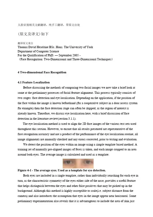
人脸识别相关文献翻译，纯手工翻译，带原文出处(原文及译文)如下翻译原文来自Thomas David Heseltine BSc. Hons. The University of YorkDepartment of Computer ScienceFor the Qualification of PhD. — September 2005 -《Face Recognition: Two-Dimensional and Three-Dimensional Techniques》4 Two-dimensional Face Recognition4.1 Feature LocalizationBefore discussing the methods of comparing two facial images we now take a brief look at some at the preliminary processes of facial feature alignment. This process typically consists of two stages: face detection and eye localisation. Depending on the application, if the position of the face within the image is known beforehand (fbr a cooperative subject in a door access system fbr example) then the face detection stage can often be skipped, as the region of interest is already known. Therefore, we discuss eye localisation here, with a brief discussion of face detection in the literature review(section 3.1.1).The eye localisation method is used to align the 2D face images of the various test sets used throughout this section. However, to ensure that all results presented are representative of the face recognition accuracy and not a product of the performance of the eye localisation routine, all image alignments are manually checked and any errors corrected, prior to testing and evaluation.We detect the position of the eyes within an image using a simple template based method. A training set of manually pre-aligned images of feces is taken, and each image cropped to an area around both eyes. The average image is calculated and used as a template.Figure 4-1 - The average eyes. Used as a template for eye detection.Both eyes are included in a single template, rather than individually searching for each eye in turn, as the characteristic symmetry of the eyes either side of the nose, provides a useful feature that helps distinguish between the eyes and other false positives that may be picked up in the background. Although this method is highly susceptible to scale(i.e. subject distance from the camera) and also introduces the assumption that eyes in the image appear near horizontal. Some preliminary experimentation also reveals that it is advantageous to include the area of skin justbeneath the eyes. The reason being that in some cases the eyebrows can closely match the template, particularly if there are shadows in the eye-sockets, but the area of skin below the eyes helps to distinguish the eyes from eyebrows (the area just below the eyebrows contain eyes, whereas the area below the eyes contains only plain skin).A window is passed over the test images and the absolute difference taken to that of the average eye image shown above. The area of the image with the lowest difference is taken as the region of interest containing the eyes. Applying the same procedure using a smaller template of the individual left and right eyes then refines each eye position.This basic template-based method of eye localisation, although providing fairly preciselocalisations, often fails to locate the eyes completely. However, we are able to improve performance by including a weighting scheme.Eye localisation is performed on the set of training images, which is then separated into two sets: those in which eye detection was successful; and those in which eye detection failed. Taking the set of successful localisations we compute the average distance from the eye template (Figure 4-2 top). Note that the image is quite dark, indicating that the detected eyes correlate closely to the eye template, as we would expect. However, bright points do occur near the whites of the eye, suggesting that this area is often inconsistent, varying greatly from the average eye template.Figure 4-2 一Distance to the eye template for successful detections (top) indicating variance due to noise and failed detections (bottom) showing credible variance due to miss-detected features.In the lower image (Figure 4-2 bottom), we have taken the set of failed localisations(images of the forehead, nose, cheeks, background etc. falsely detected by the localisation routine) and once again computed the average distance from the eye template. The bright pupils surrounded by darker areas indicate that a failed match is often due to the high correlation of the nose and cheekbone regions overwhelming the poorly correlated pupils. Wanting to emphasise the difference of the pupil regions for these failed matches and minimise the variance of the whites of the eyes for successful matches, we divide the lower image values by the upper image to produce a weights vector as shown in Figure 4-3. When applied to the difference image before summing a total error, this weighting scheme provides a much improved detection rate.Figure 4-3 - Eye template weights used to give higher priority to those pixels that best represent the eyes.4.2 The Direct Correlation ApproachWe begin our investigation into face recognition with perhaps the simplest approach,known as the direct correlation method (also referred to as template matching by Brunelli and Poggio [29 ]) involving the direct comparison of pixel intensity values taken from facial images. We use the term "Direct Conelation, to encompass all techniques in which face images are compared directly, without any form of image space analysis, weighting schemes or feature extraction, regardless of the distance metric used. Therefore, we do not infer that Pearson's correlation is applied as the similarity function (although such an approach would obviously come under our definition of direct correlation). We typically use the Euclidean distance as our metric in these investigations (inversely related to Pearson's correlation and can be considered as a scale and translation sensitive form of image correlation), as this persists with the contrast made between image space and subspace approaches in later sections.Firstly, all facial images must be aligned such that the eye centres are located at two specified pixel coordinates and the image cropped to remove any background information. These images are stored as greyscale bitmaps of 65 by 82 pixels and prior to recognition converted into a vector of 5330 elements (each element containing the corresponding pixel intensity value). Each corresponding vector can be thought of as describing a point within a 5330 dimensional image space. This simple principle can easily be extended to much larger images: a 256 by 256 pixel image occupies a single point in 65,536-dimensional image space and again, similar images occupy close points within that space. Likewise, similar faces are located close together within the image space, while dissimilar faces are spaced far apart. Calculating the Euclidean distance d, between two facial image vectors (often referred to as the query image q, and gallery image g), we get an indication of similarity. A threshold is then applied to make the final verification decision.d . q - g ( threshold accept ) (d threshold ⇒ reject ). Equ. 4-14.2.1 Verification TestsThe primary concern in any face recognition system is its ability to correctly verify a claimed identity or determine a person's most likely identity from a set of potential matches in a database. In order to assess a given system's ability to perform these tasks, a variety of evaluation methodologies have arisen. Some of these analysis methods simulate a specific mode of operation (i.e. secure site access or surveillance), while others provide a more mathematicaldescription of data distribution in some classification space. In addition, the results generated from each analysis method may be presented in a variety of formats. Throughout the experimentations in this thesis, we primarily use the verification test as our method of analysis and comparison, although we also use Fisher's Linear Discriminant to analyse individual subspace components in section 7 and the identification test for the final evaluations described in section 8. The verification test measures a system's ability to correctly accept or reject the proposed identity of an individual. At a functional level, this reduces to two images being presented for comparison, fbr which the system must return either an acceptance (the two images are of the same person) or rejection (the two images are of different people). The test is designed to simulate the application area of secure site access. In this scenario, a subject will present some form of identification at a point of entry, perhaps as a swipe card, proximity chip or PIN number. This number is then used to retrieve a stored image from a database of known subjects (often referred to as the target or gallery image) and compared with a live image captured at the point of entry (the query image). Access is then granted depending on the acceptance/rej ection decision.The results of the test are calculated according to how many times the accept/reject decision is made correctly. In order to execute this test we must first define our test set of face images. Although the number of images in the test set does not affect the results produced (as the error rates are specified as percentages of image comparisons), it is important to ensure that the test set is sufficiently large such that statistical anomalies become insignificant (fbr example, a couple of badly aligned images matching well). Also, the type of images (high variation in lighting, partial occlusions etc.) will significantly alter the results of the test. Therefore, in order to compare multiple face recognition systems, they must be applied to the same test set.However, it should also be noted that if the results are to be representative of system performance in a real world situation, then the test data should be captured under precisely the same circumstances as in the application environment.On the other hand, if the purpose of the experimentation is to evaluate and improve a method of face recognition, which may be applied to a range of application environments, then the test data should present the range of difficulties that are to be overcome. This may mean including a greater percentage of6difficult9 images than would be expected in the perceived operating conditions and hence higher error rates in the results produced. Below we provide the algorithm for executing the verification test. The algorithm is applied to a single test set of face images, using a single function call to the face recognition algorithm: CompareF aces(F ace A, FaceB). This call is used to compare two facial images, returning a distance score indicating how dissimilar the two face images are: the lower the score the more similar the two face images. Ideally, images of the same face should produce low scores, while images of different faces should produce high scores.Every image is compared with every other image, no image is compared with itself and nopair is compared more than once (we assume that the relationship is symmetrical). Once two images have been compared, producing a similarity score, the ground-truth is used to determine if the images are of the same person or different people. In practical tests this information is often encapsulated as part of the image filename (by means of a unique person identifier). Scores are then stored in one of two lists: a list containing scores produced by comparing images of different people and a list containing scores produced by comparing images of the same person. The final acceptance/rejection decision is made by application of a threshold. Any incorrect decision is recorded as either a false acceptance or false rejection. The false rejection rate (FRR) is calculated as the percentage of scores from the same people that were classified as rejections. The false acceptance rate (FAR) is calculated as the percentage of scores from different people that were classified as acceptances.For IndexA = 0 to length(TestSet) For IndexB = IndexA+l to length(TestSet) Score = CompareFaces(TestSet[IndexA], TestSet[IndexB]) If IndexA and IndexB are the same person Append Score to AcceptScoresListElseAppend Score to RejectScoresListFor Threshold = Minimum Score to Maximum Score:FalseAcceptCount, FalseRejectCount = 0For each Score in RejectScoresListIf Score <= ThresholdIncrease FalseAcceptCountFor each Score in AcceptScoresListIf Score > ThresholdIncrease FalseRejectCountF alse AcceptRate = FalseAcceptCount / Length(AcceptScoresList)FalseRej ectRate = FalseRejectCount / length(RejectScoresList)Add plot to error curve at (FalseRejectRate, FalseAcceptRate)These two error rates express the inadequacies of the system when operating at aspecific threshold value. Ideally, both these figures should be zero, but in reality reducing either the FAR or FRR (by altering the threshold value) will inevitably resultin increasing the other. Therefore, in order to describe the full operating range of a particular system, we vary the threshold value through the entire range of scores produced. The application of each threshold value produces an additional FAR, FRR pair, which when plotted on a graph produces the error rate curve shown below.False Acceptance Rate / %Figure 4-5 - Example Error Rate Curve produced by the verification test.The equal error rate (EER) can be seen as the point at which FAR is equal to FRR. This EER value is often used as a single figure representing the general recognition performance of a biometric system and allows for easy visual comparison of multiple methods. However, it is important to note that the EER does not indicate the level of error that would be expected in a real world application. It is unlikely that any real system would use a threshold value such that the percentage of false acceptances were equal to the percentage of false rejections. Secure site access systems would typically set the threshold such that false acceptances were significantly lower than false rejections: unwilling to tolerate intruders at the cost of inconvenient access denials.Surveillance systems on the other hand would require low false rejection rates to successfully identify people in a less controlled environment. Therefore we should bear in mind that a system with a lower EER might not necessarily be the better performer towards the extremes of its operating capability.There is a strong connection between the above graph and the receiver operating characteristic (ROC) curves, also used in such experiments. Both graphs are simply two visualisations of the same results, in that the ROC format uses the True Acceptance Rate(TAR), where TAR = 1.0 - FRR in place of the FRR, effectively flipping the graph vertically. Another visualisation of the verification test results is to display both the FRR and FAR as functions of the threshold value. This presentation format provides a reference to determine the threshold value necessary to achieve a specific FRR and FAR. The EER can be seen as the point where the two curves intersect.Figure 4-6 - Example error rate curve as a function of the score threshold The fluctuation of these error curves due to noise and other errors is dependant on the number of face image comparisons made to generate the data. A small dataset that only allows fbr a small number of comparisons will results in a jagged curve, in which large steps correspond to the influence of a single image on a high proportion of the comparisons made. A typical dataset of 720 images (as used in section 4.2.2) provides 258,840 verification operations, hence a drop of 1% EER represents an additional 2588 correct decisions, whereas the quality of a single image could cause the EER to fluctuate by up to 0.28.422 ResultsAs a simple experiment to test the direct correlation method, we apply the technique described above to a test set of 720 images of 60 different people, taken from the AR Face Database [ 39 ]. Every image is compared with every other image in the test set to produce a likeness score, providing 258,840 verification operations from which to calculate false acceptance rates and false rejection rates. The error curve produced is shown in Figure 4-7.Figure 4-7 - Error rate curve produced by the direct correlation method using no image preprocessing.We see that an EER of 25.1% is produced, meaning that at the EER threshold approximately one quarter of all verification operations carried out resulted in an incorrect classification. Thereare a number of well-known reasons for this poor level of accuracy. Tiny changes in lighting, expression or head orientation cause the location in image space to change dramatically. Images in face space are moved far apart due to these image capture conditions, despite being of the same person's face. The distance between images of different people becomes smaller than the area of face space covered by images of the same person and hence false acceptances and false rejections occur frequently. Other disadvantages include the large amount of storage necessaryfor holding many face images and the intensive processing required for each comparison, making this method unsuitable fbr applications applied to a large database. In section 4.3 we explore the eigenface method, which attempts to address some of these issues.4二维人脸识别4.1功能定位在讨论比较两个人脸图像，我们现在就简要介绍的方法一些在人脸特征的初步调整过程。

现代电子技术Modern Electronics TechniqueMay 2024Vol. 47 No. 102024年5月15日第47卷第10期0 引 言21世纪以来，随着智能电网的迅猛发展，电力系统成为了人们日常生活中不可或缺的一部分。

智能电网不仅直接关联着人们的用电需求，还对经济发展和国家安全具有重要影响。

在智能电网中，大量涉及用户用电数据的信息可以通过数据分析方法得以挖掘，这对于理解用户用电行为规律、用电负荷预测和防窃电检测等具有重要意义[1]。

研究用户用电行为规律对于电力系统运行和管理至关重要。

通过深入分析用户用电数据，可以揭示出不同时间段的用电负荷特征、高负荷时段以及用电行为的异常变化等信息。

这些分析结果为电力系统规划、电力调度和资源优化提供了宝贵的参考，有助于优化电力供应和提高电网运行的效率和稳定性[2]。

此外，利用用户用电数据进行负荷预测可以帮助电力系统工作人员做出准确的负荷调度安排，提前预测和应对高负荷时段的能源需求。

这对于实现电力系统的高效运行、优化能源资源利用以及提升供电质量都具有重要意义[3]。

因此，对用户用电行为规律的研究以及利用数据分析方法来挖掘和分析用户用电数据，在智能电网中具有重要的研究意义和实际应用价值。

这将为电力系统的可持续发DOI ：10.16652/j.issn.1004⁃373x.2024.10.001引用格式：李晗轲，李璟，王颖，等.用户用电负荷变化的异常检测与识别[J].现代电子技术，2024，47（10）：1⁃5.用户用电负荷变化的异常检测与识别李晗轲， 李 璟， 王 颖， 邹国平， 陈倩楠， 蔡 慧（中国计量大学 机电工程学院， 浙江 杭州 310018）摘 要： 在智能电网时代，大部分用电异常行为都会伴随用电负荷的变化，研究用户用电行为对于电力系统的运行和管理都至关重要。

为此，提出一种直接利用负荷数据进行计算，通过计算特征用电负荷曲线与日用电负荷曲线之间的相关度来判断用户是否存在异常用电行为的方法。

不同油梨品系果实品质特征的综合评价作者：徐丹刘远征张贺李艳霞马蔚红刘馨怡王甲水刘进平来源：《热带作物学报》2022年第04期摘要：本研究選用来自海南省儋州市及白沙县的9种油梨品系（DL-F、FR-1、LY-C、LY-L、RK-1、RK-2、RK-3、RK-4、RK-5）作为研究对象，分别测定其矿质元素、脂肪酸成分、维生素C、总酚、黄酮等31项重要果实品质性状，用火焰石墨炉原子吸收分光光度计测定果实中矿物质含量，采用索氏抽提法提取油梨果肉中的油脂，用气相色谱-质谱联用仪测定油脂中脂肪酸相对含量，根据国家相关标准对油梨油的理化性质进行测定，用高效液相色谱法测定维生素C，用NaNO2-AlNO3-NaOH法和酒石亚铁法测定黄酮及总酚等重要果实品质指标，并对测得的各个指标进行分析比较。

结果表明，不同油梨品系的大部分果实品质性状存在差异，9种油梨品系的油脂在密度和折射率上无显著差异，不同品系油梨含有丰富的维生素C，但其含量无显著差异;油梨果实的矿质元素含量较高，其中钾元素、磷元素以及油酸含量的测定结果与其他水果相比较，其含量较高，是评价油梨果实营养成分的重要指标。

聚类分析结果表明，在欧氏距离为5.0时，可以将9个品系聚为4大类。

第1类聚集了2个品系RK-2、RK-3，这2个品系碘价较高，皂化值很低;第2类聚集了5个品系，包括DL-F、LY-L、FR-1、RK-1、RK-4，这一类群的棕榈酸、皂化值、含水量和维生素C含量较高;第3类只有1个品系LY-C，该品系的各个指标均表现良好;第4类也只有1个品系RK-5，该品系果实品质表现较差。

综上所述，通过对海南本地不同品系油梨的多项品质性状指标进行检测，结合多种分析方法，综合分析油梨各项品质指标，可为海南地区油梨系统评价和品种改良提供参考。

关键词：油梨;果实品质;聚类分析;综合评价中图分类号：S667.9 文献标识码：AComprehensive Evaluation of Quality Characteristics of Fruit from Different Avocado StrainsXU Dan LIU Yuanzheng ZHANG He LI Yanxia MA Weihong LIU Xinyi WANG Jiashui LIU Jinping1. Haikou Experimental Station， Chinese Academy of Tropical Agricultural Sciences，Haikou， Hainan 571101， China;2. College of Tropical Crops， Hainan University， Haikou，Hainan 570228， China;3. College of Horticulture and Landscape Architecture， Tianjin Agricultural University， Tianjin 300392， ChinaAbstract：In this study， 9 avocado lines from Danzhou and Baisha， Hainan， China were selected as the research objects， namely DL-F， FR-1， LY-C， LY-L; RK-1， RK-2， RK-3，RK-4， RK-5. 31 important fruit quality traits， including mineral elements， fatty acid composition， vitamin C， total phenols， and flavonoids， of 9 varieties of avocados were determined. Graphite furnace atomic absorption spectrophotometer was used to determine the mineral content in the fruit. Soxhlet extraction was used to extract the oil in the avocado pulp. The relative contents of fatty acids in the oils and fats were determined by gas chromatography-mass spectrometry， the physicochemical properties of avocado oil were determined according to national standards， vitamin C was determined by high performance liquid chromatography， and important fruit quality indexes such as flavonoids and total phenolics were determined by NaNO2-AlNO3-NaOH method and ferrous tartrate method. Results showed that most of the fruit quality traits of different avocado lines were different. The oils of the nine lines had no significant differences in density and refractive index. The different avocado lines were rich in vitamin C， but there was no difference in its content. The fruits had a relatively high content of mineral elements. Compared with other fruits，the contents of potassium， phosphorus and oleic acid were relatively high， which is an important index for evaluating the nutritional content of avocado fruits. Cluster analysis results showed that when the Euclidean distance was 5， the varieties could be clustered into 4 categories. The first category included RK-2 and RK-3， which had high iodine value and low saponification value. The second category included DL-F， LY-L， FR-1， RK-1 and RK-4， which had higher palmitic acid， saponification value， water content and vitamin C content. The third category was LY-C，which performs well in all indicators. The fourth category was only RK-5， which had poor fruit quality. In summary， in this study， a comprehensive analysis of various quality traits of avocado was conducted in different lines from native Hainan， and several analytical methods may provide references for the systematic evaluation and variety improvement of avocado in Hainan. At the same time， the improvement and breeding of superior avocado cultivars should not only be evaluated forfruit quality， but also be combined with a wide range of indicators including disease resistance，fitness， and abundance of fruit， so that avocado cultivars with strong adaptability and suitable promotion can be screened.Keywords：avocado; fruit quality; cluster analysis; comprehensive evaluationDOI：10.3969/j.issn.1000-2561.2022.04.009油梨（Persea americana Mill.）又称为鳄梨、牛油果，为樟科（Lauraceae）鳄梨属（Persea）的常绿植物，原产于中美洲的热带、亚热带地区[1]。

Daniel D.LeeBell Laboratories Lucent Technologies Murray Hill,NJ07974H.Sebastian SeungDept.of Brain and Cog.Sci.Massachusetts Institute of TechnologyCambridge,MA02138 AbstractNon-negative matrix factorization(NMF)has previously been shown tobe a useful decomposition for multivariate data.Two different multi-plicative algorithms for NMF are analyzed.They differ only slightly inthe multiplicative factor used in the update rules.One algorithm can beshown to minimize the conventional least squares error while the otherminimizes the generalized Kullback-Leibler divergence.The monotonicconvergence of both algorithms can be proven using an auxiliary func-tion analogous to that used for proving convergence of the Expectation-Maximization algorithm.The algorithms can also be interpreted as diag-onally rescaled gradient descent,where the rescaling factor is optimallychosen to ensure convergence.1IntroductionUnsupervised learning algorithms such as principal components analysis and vector quan-tization can be understood as factorizing a data matrix subject to different constraints.De-pending upon the constraints utilized,the resulting factors can be shown to have very dif-ferent representational properties.Principal components analysis enforces only a weak or-thogonality constraint,resulting in a very distributed representation that uses cancellations to generate variability[1,2].On the other hand,vector quantization uses a hard winner-take-all constraint that results in clustering the data into mutually exclusive prototypes[3]. We have previously shown that nonnegativity is a useful constraint for matrix factorization that can learn a parts representation of the data[4,5].The nonnegative basis vectors that are learned are used in distributed,yet still sparse combinations to generate expressiveness in the reconstructions[6,7].In this submission,we analyze in detail two numerical algorithms for learning the optimal nonnegative factors from data.2Non-negative matrix factorizationWe formally consider algorithms for solving the following problem:Non-negative matrix factorization(NMF)Given a non-negative matrix,find non-negative matrix factors and such that:(1)NMF can be applied to the statistical analysis of multivariate data in the following manner. Given a set of of multivariate-dimensional data vectors,the vectors are placed in the columns of an matrix where is the number of examples in the data set.This matrix is then approximately factorized into an matrix and an matrix. Usually is chosen to be smaller than or,so that and are smaller than the original matrix.This results in a compressed version of the original data matrix.What is the significance of the approximation in Eq.(1)?It can be rewritten column by column as,where and are the corresponding columns of and.In other words,each data vector is approximated by a linear combination of the columns of, weighted by the components of.Therefore can be regarded as containing a basis that is optimized for the linear approximation of the data in.Since relatively few basis vectors are used to represent many data vectors,good approximation can only be achieved if the basis vectors discover structure that is latent in the data.The present submission is not about applications of NMF,but focuses instead on the tech-nical aspects offinding non-negative matrix factorizations.Of course,other types of ma-trix factorizations have been extensively studied in numerical linear algebra,but the non-negativity constraint makes much of this previous work inapplicable to the present case [8].Here we discuss two algorithms for NMF based on iterative updates of and.Because these algorithms are easy to implement and their convergence properties are guaranteed, we have found them very useful in practical applications.Other algorithms may possibly be more efficient in overall computation time,but are more difficult to implement and may not generalize to different cost functions.Algorithms similar to ours where only one of the factors is adapted have previously been used for the deconvolution of emission tomography and astronomical images[9,10,11,12].At each iteration of our algorithms,the new value of or is found by multiplying the current value by some factor that depends on the quality of the approximation in Eq.(1).We prove that the quality of the approximation improves monotonically with the application of these multiplicative update rules.In practice,this means that repeated iteration of the update rules is guaranteed to converge to a locally optimal matrix factorization.3Cost functionsTofind an approximate factorization,wefirst need to define cost functions that quantify the quality of the approximation.Such a cost function can be constructed using some measure of distance between two non-negative matrices and.One useful measure is simply the square of the Euclidean distance between and[13],(2)This is lower bounded by zero,and clearly vanishes if and only if.Another useful measure isWe now consider two alternative formulations of NMF as optimization problems: Problem1Minimize with respect to and,subject to the constraints .Problem2Minimize with respect to and,subject to the constraints .Although the functions and are convex in only or only,they are not convex in both variables together.Therefore it is unrealistic to expect an algorithm to solve Problems1and2in the sense offinding global minima.However,there are many techniques from numerical optimization that can be applied tofind local minima. Gradient descent is perhaps the simplest technique to implement,but convergence can be slow.Other methods such as conjugate gradient have faster convergence,at least in the vicinity of local minima,but are more complicated to implement than gradient descent [8].The convergence of gradient based methods also have the disadvantage of being very sensitive to the choice of step size,which can be very inconvenient for large applications.4Multiplicative update rulesWe have found that the following“multiplicative update rules”are a good compromise between speed and ease of implementation for solving Problems1and2.Theorem1The Euclidean distance is nonincreasing under the update rules(4)The Euclidean distance is invariant under these updates if and only if and are at a stationary point of the distance.Theorem2The divergence is nonincreasing under the update rules(5)The divergence is invariant under these updates if and only if and are at a stationary point of the divergence.Proofs of these theorems are given in a later section.For now,we note that each update consists of multiplication by a factor.In particular,it is straightforward to see that this multiplicative factor is unity when,so that perfect reconstruction is necessarily afixed point of the update rules.5Multiplicative versus additive update rulesIt is useful to contrast these multiplicative updates with those arising from gradient descent [14].In particular,a simple additive update for that reduces the squared distance can be written as(6) If are all set equal to some small positive number,this is equivalent to conventional gradient descent.As long as this number is sufficiently small,the update should reduce .Now if we diagonally rescale the variables and set(8) Again,if the are small and positive,this update should reduce.If we now setminFigure1:Minimizing the auxiliary function guarantees that for.Lemma2If is the diagonal matrix(13) then(15) Proof:Since is obvious,we need only show that.To do this,we compare(22)(23)is a positive eigenvector of with unity eigenvalue,and application of the Frobenius-Perron theorem shows that Eq.17holds.We can now demonstrate the convergence of Theorem1:Proof of Theorem1Replacing in Eq.(11)by Eq.(14)results in the update rule:(24) Since Eq.(14)is an auxiliary function,is nonincreasing under this update rule,accordingto Lemma1.Writing the components of this equation explicitly,we obtain(28)Proof:It is straightforward to verify that.To show that, we use convexity of the log function to derive the inequality(30) we obtain(31) From this inequality it follows that.Theorem2then follows from the application of Lemma1:Proof of Theorem2:The minimum of with respect to is determined by setting the gradient to zero:7DiscussionWe have shown that application of the update rules in Eqs.(4)and(5)are guaranteed to find at least locally optimal solutions of Problems1and2,respectively.The convergence proofs rely upon defining an appropriate auxiliary function.We are currently working to generalize these theorems to more complex constraints.The update rules themselves are extremely easy to implement computationally,and will hopefully be utilized by others for a wide variety of applications.We acknowledge the support of Bell Laboratories.We would also like to thank Carlos Brody,Ken Clarkson,Corinna Cortes,Roland Freund,Linda Kaufman,Yann Le Cun,Sam Roweis,Larry Saul,and Margaret Wright for helpful discussions.References[1]Jolliffe,IT(1986).Principal Component Analysis.New York:Springer-Verlag.[2]Turk,M&Pentland,A(1991).Eigenfaces for recognition.J.Cogn.Neurosci.3,71–86.[3]Gersho,A&Gray,RM(1992).Vector Quantization and Signal Compression.Kluwer Acad.Press.[4]Lee,DD&Seung,HS.Unsupervised learning by convex and conic coding(1997).Proceedingsof the Conference on Neural Information Processing Systems9,515–521.[5]Lee,DD&Seung,HS(1999).Learning the parts of objects by non-negative matrix factoriza-tion.Nature401,788–791.[6]Field,DJ(1994).What is the goal of sensory coding?Neural Comput.6,559–601.[7]Foldiak,P&Young,M(1995).Sparse coding in the primate cortex.The Handbook of BrainTheory and Neural Networks,895–898.(MIT Press,Cambridge,MA).[8]Press,WH,Teukolsky,SA,Vetterling,WT&Flannery,BP(1993).Numerical recipes:the artof scientific computing.(Cambridge University Press,Cambridge,England).[9]Shepp,LA&Vardi,Y(1982).Maximum likelihood reconstruction for emission tomography.IEEE Trans.MI-2,113–122.[10]Richardson,WH(1972).Bayesian-based iterative method of image restoration.J.Opt.Soc.Am.62,55–59.[11]Lucy,LB(1974).An iterative technique for the rectification of observed distributions.Astron.J.74,745–754.[12]Bouman,CA&Sauer,K(1996).A unified approach to statistical tomography using coordinatedescent optimization.IEEE Trans.Image Proc.5,480–492.[13]Paatero,P&Tapper,U(1997).Least squares formulation of robust non-negative factor analy-b.37,23–35.[14]Kivinen,J&Warmuth,M(1997).Additive versus exponentiated gradient updates for linearprediction.Journal of Information and Computation132,1–64.[15]Dempster,AP,Laird,NM&Rubin,DB(1977).Maximum likelihood from incomplete data viathe EM algorithm.J.Royal Stat.Soc.39,1–38.[16]Saul,L&Pereira,F(1997).Aggregate and mixed-order Markov models for statistical languageprocessing.In C.Cardie and R.Weischedel(eds).Proceedings of the Second Conference on Empirical Methods in Natural Language Processing,81–89.ACL Press.。

統計術語中英文對照[全]Absolute deviation, 絕對离差Absolute number, 絕對數Absolute residuals, 絕對殘差Acceleration array, 加速度立体陣Acceleration in an arbitrary direction, 任意方向上的加速度Acceleration normal, 法向加速度Acceleration space dimension, 加速度空間的維數Acceleration tangential, 切向加速度Acceleration vector, 加速度向量Acceptable hypothesis, 可接受假設Accumulation, 累積Accuracy, 准确度Actual frequency, 實際頻數Adaptive estimator, 自适應估計量Addition, 相加Addition theorem, 加法定理Additivity, 可加性Adjusted rate, 調整率Adjusted value, 校正值Admissible error, 容許誤差Aggregation, 聚集性Alternative hypothesis, 備擇假設Among groups, 組間Amounts, 總量Analysis of correlation, 相關分析Analysis of covariance, 協方差分析Analysis of regression, 回歸分析Analysis of time series, 時間序列分析Analysis of variance, 方差分析Angular transformation, 角轉換ANOVA （analysis of variance）, 方差分析ANOVA Models, 方差分析模型Arcing, 弧/弧旋Arcsine transformation, 反正弦變換Area under the curve, 曲線面積AREG , 評估從一個時間點到下一個時間點回歸相關時的誤差ARIMA, 季節和非季節性單變量模型的极大似然估計Arithmetic grid paper, 算術格紙Arithmetic mean, 算術平均數Arrhenius relation, 艾恩尼斯關系Assessing fit, 擬合的評估Associative laws, 結合律Asymmetric distribution, 非對稱分布Asymptotic bias, 漸近偏倚Asymptotic efficiency, 漸近效率Asymptotic variance, 漸近方差Attributable risk, 歸因危險度Attribute data, 屬性資料Attribution, 屬性Autocorrelation, 自相關Autocorrelation of residuals, 殘差的自相關Average, 平均數Average confidence interval length, 平均置信區間長度Average growth rate, 平均增長率Bar chart, 條形圖Bar graph, 條形圖Base period, 基期Bayes' theorem , Bayes定理Bell-shaped curve, 鐘形曲線Bernoulli distribution, 伯努力分布Best-trim estimator, 最好切尾估計量Bias, 偏性Binary logistic regression, 二元邏輯斯蒂回歸Binomial distribution, 二項分布Bisquare, 雙平方Bivariate Correlate, 二變量相關Bivariate normal distribution, 雙變量正態分布Bivariate normal population, 雙變量正態總体Biweight interval, 雙權區間Biweight M-estimator, 雙權M估計量Block, 區組/配伍組BMDP(Biomedical computer programs), BMDP統計軟件包Boxplots, 箱線圖/箱尾圖Breakdown bound, 崩潰界/崩潰點Canonical correlation, 典型相關Caption, 縱標目Case-control study, 病例對照研究Categorical variable, 分類變量Catenary, 懸鏈線Cauchy distribution, 柯西分布Cause-and-effect relationship, 因果關系Cell, 單元Censoring, 終檢Center of symmetry, 對稱中心Centering and scaling, 中心化和定標Central tendency, 集中趨勢Central value, 中心值CHAID -χ2 Automatic Interaction Detector, 卡方自動交互檢測Chance, 机遇Chance error, 隨机誤差Chance variable, 隨机變量Characteristic equation, 特征方程Characteristic root, 特征根Characteristic vector, 特征向量Chebshev criterion of fit, 擬合的切比雪夫准則Chernoff faces, 切爾諾夫臉譜圖Chi-square test, 卡方檢驗/χ2檢驗Choleskey decomposition, 喬洛斯基分解Circle chart, 圓圖Class interval, 組距Class mid-value, 組中值Class upper limit, 組上限Classified variable, 分類變量Cluster analysis, 聚類分析Cluster sampling, 整群抽樣Code, 代碼Coded data, 編碼數据Coding, 編碼Coefficient of contingency, 列聯系數Coefficient of determination, 決定系數Coefficient of multiple correlation, 多重相關系數Coefficient of partial correlation, 偏相關系數Coefficient of production-moment correlation, 積差相關系數Coefficient of rank correlation, 等級相關系數Coefficient of regression, 回歸系數Coefficient of skewness, 偏度系數Coefficient of variation, 變异系數Cohort study, 隊列研究Column, 列Column effect, 列效應Column factor, 列因素Combination pool, 合并Combinative table, 組合表Common factor, 共性因子Common regression coefficient, 公共回歸系數Common value, 共同值Common variance, 公共方差Common variation, 公共變异Communality variance, 共性方差Comparability, 可比性Comparison of bathes, 批比較Comparison value, 比較值Compartment model, 分部模型Compassion, 伸縮Complement of an event, 補事件Complete association, 完全正相關Complete dissociation, 完全不相關Complete statistics, 完備統計量Completely randomized design, 完全隨机化設計Composite event, 聯合事件Composite events, 复合事件Concavity, 凹性Conditional expectation, 條件期望Conditional likelihood, 條件似然Conditional probability, 條件概率Conditionally linear, 依條件線性Confidence interval, 置信區間Confidence limit, 置信限Confidence lower limit, 置信下限Confidence upper limit, 置信上限Confirmatory Factor Analysis , 驗證性因子分析Confirmatory research, 證實性實驗研究Confounding factor, 混雜因素Conjoint, 聯合分析Consistency, 相合性Consistency check, 一致性檢驗Consistent asymptotically normal estimate, 相合漸近正態估計Consistent estimate, 相合估計Constrained nonlinear regression, 受約束非線性回歸Constraint, 約束Contaminated distribution, 污染分布Contaminated Gausssian, 污染高斯分布Contaminated normal distribution, 污染正態分布Contamination, 污染Contamination model, 污染模型Contingency table, 列聯表Contour, 邊界線Contribution rate, 貢獻率Control, 對照Controlled experiments, 對照實驗Conventional depth, 常規深度Convolution, 卷積Corrected factor, 校正因子Corrected mean, 校正均值Correction coefficient, 校正系數Correctness, 正确性Correlation coefficient, 相關系數Correlation index, 相關指數Correspondence, 對應Counting, 計數Counts, 計數/頻數Covariance, 協方差Covariant, 共變Cox Regression, Cox回歸Criteria for fitting, 擬合准則Criteria of least squares, 最小二乘准則Critical ratio, 臨界比Critical region, 拒絕域Critical value, 臨界值Cross-over design, 交叉設計Cross-section analysis, 橫斷面分析Cross-section survey, 橫斷面調查Crosstabs , 交叉表Cross-tabulation table, 复合表Cube root, 立方根Cumulative distribution function, 分布函數Cumulative probability, 累計概率Curvature, 曲率/彎曲Curvature, 曲率Curve fit , 曲線擬和Curve fitting, 曲線擬合Curvilinear regression, 曲線回歸Curvilinear relation, 曲線關系Cut-and-try method, 嘗試法Cycle, 周期Cyclist, 周期性D test, D檢驗Data acquisition, 資料收集Data bank, 數据庫Data capacity, 數据容量Data deficiencies, 數据缺乏Data handling, 數据處理Data manipulation, 數据處理Data processing, 數据處理Data reduction, 數据縮減Data set, 數据集Data sources, 數据來源Data transformation, 數据變換Data validity, 數据有效性Data-in, 數据輸入Data-out, 數据輸出Dead time, 停滯期Degree of freedom, 自由度Degree of precision, 精密度Degree of reliability, 可靠性程度Degression, 遞減Density function, 密度函數Density of data points, 數据點的密度Dependent variable, 應變量/依變量/因變量Dependent variable, 因變量Depth, 深度Derivative matrix, 導數矩陣Derivative-free methods, 無導數方法Design, 設計Determinacy, 确定性Determinant, 行列式Determinant, 決定因素Deviation, 离差Deviation from average, 离均差Diagnostic plot, 診斷圖Dichotomous variable, 二分變量Differential equation, 微分方程Direct standardization, 直接標准化法Discrete variable, 离散型變量DISCRIMINANT, 判斷Discriminant analysis, 判別分析Discriminant coefficient, 判別系數Discriminant function, 判別值Dispersion, 散布/分散度Disproportional, 不成比例的Disproportionate sub-class numbers, 不成比例次級組含量Distribution free, 分布無關性/免分布Distribution shape, 分布形狀Distribution-free method, 任意分布法Distributive laws, 分配律Disturbance, 隨机扰動項Dose response curve, 劑量反應曲線Double blind method, 雙盲法Double blind trial, 雙盲試驗Double exponential distribution, 雙指數分布Double logarithmic, 雙對數Downward rank, 降秩Dual-space plot, 對偶空間圖DUD, 無導數方法Duncan's new multiple range method, 新复极差法/Duncan新法Effect, 實驗效應Eigenvalue, 特征值Eigenvector, 特征向量Ellipse, 橢圓Empirical distribution, 經驗分布Empirical probability, 經驗概率單位Enumeration data, 計數資料Equal sun-class number, 相等次級組含量Equally likely, 等可能Equivariance, 同變性Error, 誤差/錯誤Error of estimate, 估計誤差Error type I, 第一類錯誤Error type II, 第二類錯誤Estimand, 被估量Estimated error mean squares, 估計誤差均方Estimated error sum of squares, 估計誤差平方和Euclidean distance, 歐式距离Event, 事件Event, 事件Exceptional data point, 异常數据點Expectation plane, 期望平面Expectation surface, 期望曲面Expected values, 期望值Experiment, 實驗Experimental sampling, 試驗抽樣Experimental unit, 試驗單位Explanatory variable, 說明變量Exploratory data analysis, 探索性數据分析Explore Summarize, 探索-摘要Exponential curve, 指數曲線Exponential growth, 指數式增長EX SMOOTH, 指數平滑方法Extended fit, 擴充擬合Extra parameter, 附加參數Extrapolation, 外推法Extreme observation, 末端觀測值Extremes, 极端值/极值F distribution, F分布F test, F檢驗Factor, 因素/因子Factor analysis, 因子分析Factor Analysis, 因子分析Factor score, 因子得分Factorial, 階乘Factorial design, 析因試驗設計False negative, 假陰性False negative error, 假陰性錯誤Family of distributions, 分布族Family of estimators, 估計量族Fanning, 扇面Fatality rate, 病死率Field investigation, 現場調查Field survey, 現場調查Finite population, 有限總体Finite-sample, 有限樣本First derivative, 一階導數First principal component, 第一主成分First quartile, 第一四分位數Fisher information, 費雪信息量Fitted value, 擬合值Fitting a curve, 曲線擬合Fixed base, 定基Fluctuation, 隨机起伏Forecast, 預測Four fold table, 四格表Fourth, 四分點Fraction blow, 左側比率Fractional error, 相對誤差Frequency, 頻率Frequency polygon, 頻數多邊圖Frontier point, 界限點Function relationship, 泛函關系Gamma distribution, 伽瑪分布Gauss increment, 高斯增量Gaussian distribution, 高斯分布/正態分布Gauss-Newton increment, 高斯-牛頓增量General census, 全面普查GENLOG (Generalized liner models), 廣義線性模型Geometric mean, 几何平均數Gini's mean difference, 基尼均差GLM (General liner models), 通用線性模型Goodness of fit, 擬和优度/配合度Gradient of determinant, 行列式的梯度Graeco-Latin square, 希腊拉丁方Grand mean, 總均值Gross errors, 重大錯誤Gross-error sensitivity, 大錯敏感度Group averages, 分組平均Grouped data, 分組資料Guessed mean, 假定平均數Half-life, 半衰期Hampel M-estimators, 漢佩爾M估計量Happenstance, 偶然事件Harmonic mean, 調和均數Hazard function, 風險均數Hazard rate, 風險率Heading, 標目Heavy-tailed distribution, 重尾分布Hessian array, 海森立体陣Heterogeneity, 不同質Heterogeneity of variance, 方差不齊Hierarchical classification, 組內分組Hierarchical clustering method, 系統聚類法High-leverage point, 高杠杆率點HILOGLINEAR, 多維列聯表的層次對數線性模型Hinge, 折葉點Histogram, 直方圖Historical cohort study, 歷史性隊列研究Holes, 空洞HOMALS, 多重響應分析Homogeneity of variance, 方差齊性Homogeneity test, 齊性檢驗Huber M-estimators, 休伯M估計量Hyperbola, 雙曲線Hypothesis testing, 假設檢驗Hypothetical universe, 假設總体Impossible event, 不可能事件Independence, 獨立性Independent variable, 自變量Index, 指標/指數Indirect standardization, 間接標准化法Individual, 個体Inference band, 推斷帶Infinite population, 無限總体Infinitely great, 無窮大Infinitely small, 無窮小Influence curve, 影響曲線Information capacity, 信息容量Initial condition, 初始條件Initial estimate, 初始估計值Initial level, 最初水平Interaction, 交互作用Interaction terms, 交互作用項Intercept, 截距Interpolation, 內插法Interquartile range, 四分位距Interval estimation, 區間估計Intervals of equal probability, 等概率區間Intrinsic curvature, 固有曲率Invariance, 不變性Inverse matrix, 逆矩陣Inverse probability, 逆概率Inverse sine transformation, 反正弦變換Iteration, 迭代Jacobian determinant, 雅可比行列式Joint distribution function, 分布函數Joint probability, 聯合概率Joint probability distribution, 聯合概率分布K means method, 逐步聚類法Kaplan-Meier, 評估事件的時間長度Kaplan-Merier chart, Kaplan-Merier圖Kendall's rank correlation, Kendall等級相關Kinetic, 動力學Kolmogorov-Smirnove test, 柯爾莫哥洛夫-斯米爾諾夫檢驗Kruskal and Wallis test, Kruskal及Wallis檢驗/多樣本的秩和檢驗/H檢驗Kurtosis, 峰度Lack of fit, 失擬Ladder of powers, 冪階梯Lag, 滯后Large sample, 大樣本Large sample test, 大樣本檢驗Latin square, 拉丁方Latin square design, 拉丁方設計Leakage, 泄漏Least favorable configuration, 最不利构形Least favorable distribution, 最不利分布Least significant difference, 最小顯著差法Least square method, 最小二乘法Least-absolute-residuals estimates, 最小絕對殘差估計Least-absolute-residuals fit, 最小絕對殘差擬合Least-absolute-residuals line, 最小絕對殘差線Legend, 圖例L-estimator, L估計量L-estimator of location, 位置L估計量L-estimator of scale, 尺度L估計量Level, 水平Life expectance, 預期期望壽命Life table, 壽命表Life table method, 生命表法Light-tailed distribution, 輕尾分布Likelihood function, 似然函數Likelihood ratio, 似然比line graph, 線圖Linear correlation, 直線相關Linear equation, 線性方程Linear programming, 線性規划Linear regression, 直線回歸Linear Regression, 線性回歸Linear trend, 線性趨勢Loading, 載荷Location and scale equivariance, 位置尺度同變性Location equivariance, 位置同變性Location invariance, 位置不變性Location scale family, 位置尺度族Log rank test, 時序檢驗Logarithmic curve, 對數曲線Logarithmic normal distribution, 對數正態分布Logarithmic scale, 對數尺度Logarithmic transformation, 對數變換Logic check, 邏輯檢查Logistic distribution, 邏輯斯特分布Logit transformation, Logit轉換LOGLINEAR, 多維列聯表通用模型Lognormal distribution, 對數正態分布Lost function, 損失函數Low correlation, 低度相關Lower limit, 下限Lowest-attained variance, 最小可達方差LSD, 最小顯著差法的簡稱Lurking variable, 潛在變量Main effect, 主效應Major heading, 主辭標目Marginal density function, 邊緣密度函數Marginal probability, 邊緣概率Marginal probability distribution, 邊緣概率分布Matched data, 配對資料Matched distribution, 匹配過分布Matching of distribution, 分布的匹配Matching of transformation, 變換的匹配Mathematical expectation, 數學期望Mathematical model, 數學模型Maximum L-estimator, 极大极小L 估計量Maximum likelihood method, 最大似然法Mean, 均數Mean squares between groups, 組間均方Mean squares within group, 組內均方Means (Compare means), 均值-均值比較Median, 中位數Median effective dose, 半數效量Median lethal dose, 半數致死量Median polish, 中位數平滑Median test, 中位數檢驗Minimal sufficient statistic, 最小充分統計量Minimum distance estimation, 最小距离估計Minimum effective dose, 最小有效量Minimum lethal dose, 最小致死量Minimum variance estimator, 最小方差估計量MINITAB, 統計軟件包Minor heading, 賓詞標目Missing data, 缺失值Model specification, 模型的确定Modeling Statistics , 模型統計Models for outliers, 离群值模型Modifying the model, 模型的修正Modulus of continuity, 連續性模Morbidity, 發病率Most favorable configuration, 最有利构形Multidimensional Scaling (ASCAL), 多維尺度/多維標度Multinomial Logistic Regression , 多項邏輯斯蒂回歸Multiple comparison, 多重比較Multiple correlation , 复相關Multiple covariance, 多元協方差Multiple linear regression, 多元線性回歸Multiple response , 多重選項Multiple solutions, 多解Multiplication theorem, 乘法定理Multiresponse, 多元響應Multi-stage sampling, 多階段抽樣Multivariate T distribution, 多元T分布Mutual exclusive, 互不相容Mutual independence, 互相獨立Natural boundary, 自然邊界Natural dead, 自然死亡Natural zero, 自然零Negative correlation, 負相關Negative linear correlation, 負線性相關Negatively skewed, 負偏Newman-Keuls method, q檢驗NK method, q檢驗No statistical significance, 無統計意義Nominal variable, 名義變量Nonconstancy of variability, 變异的非定常性Nonlinear regression, 非線性相關Nonparametric statistics, 非參數統計Nonparametric test, 非參數檢驗Nonparametric tests, 非參數檢驗Normal deviate, 正態离差Normal distribution, 正態分布Normal equation, 正規方程組Normal ranges, 正常范圍Normal value, 正常值Nuisance parameter, 多余參數/討厭參數Null hypothesis, 無效假設Numerical variable, 數值變量Objective function, 目標函數Observation unit, 觀察單位Observed value, 觀察值One sided test, 單側檢驗One-way analysis of variance, 單因素方差分析Oneway ANOVA , 單因素方差分析Open sequential trial, 開放型序貫設計Optrim, 优切尾Optrim efficiency, 优切尾效率Order statistics, 順序統計量Ordered categories, 有序分類Ordinal logistic regression , 序數邏輯斯蒂回歸Ordinal variable, 有序變量Orthogonal basis, 正交基Orthogonal design, 正交試驗設計Orthogonality conditions, 正交條件ORTHOPLAN, 正交設計Outlier cutoffs, 离群值截斷點Outliers, 极端值OVERALS , 多組變量的非線性正規相關Overshoot, 迭代過度Paired design, 配對設計Paired sample, 配對樣本Pairwise slopes, 成對斜率Parabola, 拋物線Parallel tests, 平行試驗Parameter, 參數Parametric statistics, 參數統計Parametric test, 參數檢驗Partial correlation, 偏相關Partial regression, 偏回歸Partial sorting, 偏排序Partials residuals, 偏殘差Pattern, 模式Pearson curves, 皮爾遜曲線Peeling, 退層Percent bar graph, 百分條形圖Percentage, 百分比Percentile, 百分位數Percentile curves, 百分位曲線Periodicity, 周期性Permutation, 排列P-estimator, P估計量Pie graph, 餅圖Pitman estimator, 皮特曼估計量Pivot, 樞軸量Planar, 平坦Planar assumption, 平面的假設PLANCARDS, 生成試驗的計划卡Point estimation, 點估計Poisson distribution, 泊松分布Polishing, 平滑Polled standard deviation, 合并標准差Polled variance, 合并方差Polygon, 多邊圖Polynomial, 多項式Polynomial curve, 多項式曲線Population, 總体Population attributable risk, 人群歸因危險度Positive correlation, 正相關Positively skewed, 正偏Posterior distribution, 后驗分布Power of a test, 檢驗效能Precision, 精密度Predicted value, 預測值Preliminary analysis, 預備性分析Principal component analysis, 主成分分析Prior distribution, 先驗分布Prior probability, 先驗概率Probabilistic model, 概率模型probability, 概率Probability density, 概率密度Product moment, 乘積矩/協方差Profile trace, 截面跡圖Proportion, 比/构成比Proportion allocation in stratified random sampling, 按比例分層隨机抽樣Proportionate, 成比例Proportionate sub-class numbers, 成比例次級組含量Prospective study, 前瞻性調查Proximities, 親近性Pseudo F test, 近似F檢驗Pseudo model, 近似模型Pseudosigma, 偽標准差Purposive sampling, 有目的抽樣QR decomposition, QR分解Quadratic approximation, 二次近似Qualitative classification, 屬性分類Qualitative method, 定性方法Quantile-quantile plot, 分位數-分位數圖/Q-Q圖Quantitative analysis, 定量分析Quartile, 四分位數Quick Cluster, 快速聚類Radix sort, 基數排序Random allocation, 隨机化分組Random blocks design, 隨机區組設計Random event, 隨机事件Randomization, 隨机化Range, 极差/全距Rank correlation, 等級相關Rank sum test, 秩和檢驗Rank test, 秩檢驗Ranked data, 等級資料Rate, 比率Ratio, 比例Raw data, 原始資料Raw residual, 原始殘差Rayleigh's test, 雷氏檢驗Rayleigh's Z, 雷氏Z值Reciprocal, 倒數Reciprocal transformation, 倒數變換Recording, 記錄Redescending estimators, 回降估計量Reducing dimensions, 降維Re-expression, 重新表達Reference set, 標准組Region of acceptance, 接受域Regression coefficient, 回歸系數Regression sum of square, 回歸平方和Rejection point, 拒絕點Relative dispersion, 相對离散度Relative number, 相對數Reliability, 可靠性Reparametrization, 重新設置參數Replication, 重复Report Summaries, 報告摘要Residual sum of square, 剩余平方和Resistance, 耐抗性Resistant line, 耐抗線Resistant technique, 耐抗技術R-estimator of location, 位置R估計量R-estimator of scale, 尺度R估計量Retrospective study, 回顧性調查Ridge trace, 岭跡Ridit analysis, Ridit分析Rotation, 旋轉Rounding, 舍入Row, 行Row effects, 行效應Row factor, 行因素RXC table, RXC表Sample, 樣本Sample regression coefficient, 樣本回歸系數Sample size, 樣本量Sample standard deviation, 樣本標准差Sampling error, 抽樣誤差SAS(Statistical analysis system ), SAS統計軟件包Scale, 尺度/量表Scatter diagram, 散點圖Schematic plot, 示意圖/簡圖Score test, 計分檢驗Screening, 篩檢SEASON, 季節分析Second derivative, 二階導數Second principal component, 第二主成分SEM (Structural equation modeling), 結构化方程模型Semi-logarithmic graph, 半對數圖Semi-logarithmic paper, 半對數格紙Sensitivity curve, 敏感度曲線Sequential analysis, 貫序分析Sequential data set, 順序數据集Sequential design, 貫序設計Sequential method, 貫序法Sequential test, 貫序檢驗法Serial tests, 系列試驗Short-cut method, 簡捷法Sigmoid curve, S形曲線Sign function, 正負號函數Sign test, 符號檢驗Signed rank, 符號秩Significance test, 顯著性檢驗Significant figure, 有效數字Simple cluster sampling, 簡單整群抽樣Simple correlation, 簡單相關Simple random sampling, 簡單隨机抽樣Simple regression, 簡單回歸simple table, 簡單表Sine estimator, 正弦估計量Single-valued estimate, 單值估計Singular matrix, 奇异矩陣Skewed distribution, 偏斜分布Skewness, 偏度Slash distribution, 斜線分布Slope, 斜率Smirnov test, 斯米爾諾夫檢驗Source of variation, 變异來源Spearman rank correlation, 斯皮爾曼等級相關Specific factor, 特殊因子Specific factor variance, 特殊因子方差Spectra , 頻譜Spherical distribution, 球型正態分布Spread, 展布SPSS(Statistical package for the social science), SPSS統計軟件包Spurious correlation, 假性相關Square root transformation, 平方根變換Stabilizing variance, 穩定方差Standard deviation, 標准差Standard error, 標准誤Standard error of difference, 差別的標准誤Standard error of estimate, 標准估計誤差Standard error of rate, 率的標准誤Standard normal distribution, 標准正態分布Standardization, 標准化Starting value, 起始值Statistic, 統計量Statistical control, 統計控制Statistical graph, 統計圖Statistical inference, 統計推斷Statistical table, 統計表Steepest descent, 最速下降法Stem and leaf display, 莖葉圖Step factor, 步長因子Stepwise regression, 逐步回歸Storage, 存Strata, 層（复數）Stratified sampling, 分層抽樣Stratified sampling, 分層抽樣Strength, 強度Stringency, 嚴密性Structural relationship, 結构關系Studentized residual, 學生化殘差/t化殘差Sub-class numbers, 次級組含量Subdividing, 分割Sufficient statistic, 充分統計量Sum of products, 積和Sum of squares, 离差平方和Sum of squares about regression, 回歸平方和Sum of squares between groups, 組間平方和Sum of squares of partial regression, 偏回歸平方和Sure event, 必然事件Survey, 調查Survival, 生存分析Survival rate, 生存率Suspended root gram, 懸吊根圖Symmetry, 對稱Systematic error, 系統誤差Systematic sampling, 系統抽樣Tags, 標簽Tail area, 尾部面積Tail length, 尾長Tail weight, 尾重Tangent line, 切線Target distribution, 目標分布Taylor series, 泰勒級數Tendency of dispersion, 离散趨勢Testing of hypotheses, 假設檢驗Theoretical frequency, 理論頻數Time series, 時間序列Tolerance interval, 容忍區間Tolerance lower limit, 容忍下限Tolerance upper limit, 容忍上限Torsion, 扰率Total sum of square, 總平方和Total variation, 總變异Transformation, 轉換Treatment, 處理Trend, 趨勢Trend of percentage, 百分比趨勢Trial, 試驗Trial and error method, 試錯法Tuning constant, 細調常數Two sided test, 雙向檢驗Two-stage least squares, 二階最小平方Two-stage sampling, 二階段抽樣Two-tailed test, 雙側檢驗Two-way analysis of variance, 雙因素方差分析Two-way table, 雙向表Type I error, 一類錯誤/α錯誤Type II error, 二類錯誤/β錯誤UMVU, 方差一致最小無偏估計簡稱Unbiased estimate, 無偏估計Unconstrained nonlinear regression , 無約束非線性回歸Unequal subclass number, 不等次級組含量Ungrouped data, 不分組資料Uniform coordinate, 均勻坐標Uniform distribution, 均勻分布Uniformly minimum variance unbiased estimate, 方差一致最小無偏估計Unit, 單元Unordered categories, 無序分類Upper limit, 上限Upward rank, 升秩Vague concept, 模糊概念Validity, 有效性VARCOMP (Variance component estimation), 方差元素估計Variability, 變异性Variable, 變量Variance, 方差Variation, 變异Varimax orthogonal rotation, 方差最大正交旋轉Volume of distribution, 容積W test, W檢驗Weibull distribution, 威布爾分布Weight, 權數Weighted Chi-square test, 加權卡方檢驗/Cochran檢驗Weighted linear regression method, 加權直線回歸Weighted mean, 加權平均數Weighted mean square, 加權平均方差Weighted sum of square, 加權平方和Weighting coefficient, 權重系數Weighting method, 加權法W-estimation, W估計量W-estimation of location, 位置W估計量Width, 寬度Wilcoxon paired test, 威斯康星配對法/配對符號秩和檢驗Wild point, 野點/狂點Wild value, 野值/狂值Winsorized mean, 縮尾均值Withdraw, 失訪Youden's index, 尤登指數Z test, Z檢驗Zero correlation, 零相關Z-transformation, Z變換。

引用格式：王舒文, 章圣意, 林新霞, 等. 超声换能器动态性能一致性评估方法[J]. 中国测试，2023, 49(7): 118-124. WANG Shuwen, ZHANG Shengyi, LIN Xinxia, et al. Evaluation method of dynamic performance consistency of ultrasonic transducer[J].China Measurement & Test, 2023, 49(7): 118-124. DOI: 10.11857/j.issn.1674-5124.2022010013超声换能器动态性能一致性评估方法王舒文1， 章圣意2， 林新霞2， 林 恒2， 卜勤超3， 赵伟国1(1. 中国计量大学计量测试工程学院，浙江 杭州 310018; 2. 浙江苍南仪表集团股份有限公司，浙江 苍南 325800;3. 上海裕达实业有限公司，上海 200240)摘　要: 超声换能器是超声流量计中的核心传感器件，其动态性能决定超声流量计的计量准确性。

针对此问题，提出一种超声换能器动态性能测试方法，并对一致性进行评估。

该方法通过高斯模型和人工鱼群算法实现回波信号特征参数的最优估计，建立超声换能器的动态回波模型，并根据各超声换能器之间的回波特征参数计算欧氏距离，实现超声换能器的一致性评估。

流量实验结果表明，当超声换能器的欧氏距离减小时，零流量读数小于±0.012 m/s ，小流量的重复性优于0.2%，验证评估方法的可行性。

关键词: 超声换能器; 动态性能; 一致性评估; 流量测量中图分类号: TH814;TB9文献标志码: A文章编号: 1674–5124(2023)07–0118–07Evaluation method of dynamic performance consistency of ultrasonic transducerWANG Shuwen 1, ZHANG Shengyi 2, LIN Xinxia 2, LIN Heng 2, BU Qinchao 3, ZHAO Weiguo 1(1. College of Metrological and Measurement Engineering, China Jiliang University, Hangzhou 310018, China;2. Zhejiang Cangnan lnstrument Group Co., Ltd., Cangnan 325800, China;3. Shanghai YuDa Industrial Co., Ltd., Shanghai 200240, China)Abstract : Ultrasonic transducer is the core sensor of ultrasonic flowmeter and its dynamic performance determines the measurement accuracy of ultrasonic flowmeter. In order to solve this problem, a dynamic performance method of ultrasonic transducer is proposed and their consistency is evaluated. The Gaussian model and artificial fish-swarm algorithm are used to get the optimal estimation of echo signal characteristic parameters. The dynamic echo model of ultrasonic transducers is established. The Euclidean distance is adoped to calculated the consistency according to the echo characteristic parameters between ultrasonic transducers.Finally, the zero flowrate values are less than ±0.012 m/s and the repeatability of small flowrate is less than 0.2% when the ultrasonic transducers of the smaller Euclidean distance are used in the experiments. The feasibility of the evaluation method is verified.Keywords : keys:ultrasonic transducer; dynamic performance; consistency assessment; flow measurement收稿日期: 2022-01-04；收到修改稿日期: 2022-02-10基金项目: 国家市场监督管理总局科技计划项目(2019MK146)作者简介: 王舒文（1996- ），男，浙江杭州市人，硕士研究生，专业方向为流量计量测试和智能化仪表。

兰州交通大学硕士学位论文摘要机械设备故障诊断中，由于机械设备本身结构复杂，加之环境噪声的干扰，导致反映设备运行状态的信息常常被强噪声淹没。

尤其是在机械设备故障早期阶段，提取微弱故障特征更加困难。

此外，故障诊断所需信号主要由布置在结构上的传感器提供，传感器如何布局对故障信号获取及诊断结果至关重要。

本文从振动信号采集和处理的角度出发，针对采集过程中测点优化以及早期微弱故障的诊断两方面展开了研究，前者以泵体测点优化布置为例，后者以轴承故障诊断为例。

主要工作如下：以获取用于故障诊断的最佳信息为目标，实现用有限数量的传感器获得大量信息的同时最大限度的降低冗余信息，采用模糊C均值聚类方法，实现传感器优化布置。

首先，对结构进行模态分析，提取模态振型；其次，根据结构各自由度在重要模态中振型的动力相似性，用模糊C均值聚类对自由度进行分类，从各聚类自由度中筛选出信息较丰富的自由度作为待选测点，基于模态置信准则(modal assurance criterion, MAC)建立目标函数，采用遗传算法进行寻优，实现传感器位置的优化；最后，由模态矩阵奇异值比、Fisher 信息准则、MAC准则三个评价准则构成综合评价指标，对不同的布置结果进行评价。

以某机车泵体为例，仿真结果表明：该方法能在获得大量反映设备运行状态信息的同时有效避免测点聚集，解决了信息冗余问题。

引入改进奇异值分解(singular value decomposition, SVD)及参数优化变分模态分解(variational mode decomposition, VMD)方法，进行早期微弱故障诊断。

首先对原始故障信号进行SVD降噪、微弱故障信号分离，通过包络熵最小、峭度最大原则对其重构矩阵的秩进行优化；其次，对改进SVD降噪后所得信号进行VMD分解，将包络谱幅值峭度和峭度构成新的指标（合成峭度），通过所有本征模态分量(intrinsic mode function, IMF)的合成峭度均值最大原则对VMD的参数进行优化，获得若干IMFs；最后，根据峭度-欧氏距离指标筛选出含故障信息丰富的IMF，求取该IMF的包络谱，将幅值突出处的特征频率与理论值作对比，判断故障类型。

使⽤Matlab计算各种距离Distance计算距离的需求有两种： ⼀种是给定⼀个特征集合X，然后计算Pairwise距离矩阵，那么可使⽤D=pdist(X,distance)的⽅式； 另⼀种是给定两个对应的特征集合X和Y，然后计算X与Y对应的距离信息，使⽤D=pdist2(X,Y,distance)的⽅式；需注意，2011版本以前的Matlab是没有pdist2.m⽂件的，⽽早期的pdist2.m⽂件中的距离计算⽅式也⽐较少，所以建议使⽤最新的Matlab版本，很重要。

其中，distance的定义有如下⼏种：欧⼏⾥德距离Euclidean distance(‘euclidean’)欧⽒距离虽然很有⽤，但也有明显的缺点。

⼀：它将样品的不同属性（即各指标或各变量）之间的差别等同看待，这⼀点有时不能满⾜实际要求。

⼆：它没有考虑各变量的数量级(量纲)，容易犯⼤数吃⼩数的⽑病。

所以，可以先对原始数据进⾏规范化处理再进⾏距离计算。

标准欧⼏⾥德距离Standardized Euclidean distance(‘seuclidean’)相⽐单纯的欧⽒距离，标准欧⽒距离能够有效的解决上述缺点。

注意，这⾥的V在许多Matlab函数中是可以⾃⼰设定的，不⼀定⾮得取标准差，可以依据各变量的重要程度设置不同的值，如knnsearch函数中的Scale属性。

马哈拉诺⽐斯距离Mahalanobis distance(‘mahalanobis’)where C is the covariance matrix.马⽒距离是由印度统计学家马哈拉诺⽐斯(P. C. Mahalanobis)提出的，表⽰数据的协⽅差距离。

它是⼀种有效的计算两个未知样本集的相似度的⽅法。

与欧式距离不同的是它考虑到各种特性之间的联系（例如：⼀条关于⾝⾼的信息会带来⼀条关于体重的信息，因为两者是有关联的）并且是尺度⽆关的(scale-invariant)，即独⽴于测量尺度。

统计学专业名词·中英对照Lansexyhttp：//hi。

baidu。

com/new/lansexy我大学毕业已经多年,这些年来,越发感到外刊的重要性.读懂外刊要有不错的英语功底，同时,还需要掌握一定的专业词汇。

掌握足够的专业词汇，在国内外期刊的阅读和写作中会游刃有余。

在此小结，按首字母顺序排列。

这些词汇的来源，一是专业书籍，二是网上查找，再一个是比较重要的期刊。

当然,这些仅是常用专业词汇的一部分，并且由于个人精力、文献查阅的限制，难免有不足和错误之处，希望读者批评指出.Aabscissa 横坐标absence rate 缺勤率Absolute deviation 绝对离差Absolute number 绝对数absolute value 绝对值Absolute residuals 绝对残差accident error 偶然误差Acceleration array 加速度立体阵Acceleration in an arbitrary direction 任意方向上的加速度Acceleration normal 法向加速度Acceleration space dimension 加速度空间的维数Acceleration tangential 切向加速度Acceleration vector 加速度向量Acceptable hypothesis 可接受假设Accumulation 累积Accumulated frequency 累积频数Accuracy 准确度Actual frequency 实际频数Adaptive estimator 自适应估计量Addition 相加Addition theorem 加法定理Additive Noise 加性噪声Additivity 可加性Adjusted rate 调整率Adjusted value 校正值Admissible error 容许误差Aggregation 聚集性Alpha factoring α因子法Alternative hypothesis 备择假设Among groups 组间Amounts 总量Analysis of correlation 相关分析Analysis of covariance 协方差分析Analysis of data 分析资料Analysis Of Effects 效应分析Analysis Of Variance 方差分析Analysis of regression 回归分析Analysis of time series 时间序列分析Analysis of variance 方差分析Angular transformation 角转换ANOVA （analysis of variance）方差分析ANOVA Models 方差分析模型ANOVA table and eta 分组计算方差分析Arcing 弧/弧旋Arcsine transformation 反正弦变换Area 区域图Area under the curve 曲线面积AREG 评估从一个时间点到下一个时间点回归相关时的误差ARIMA 季节和非季节性单变量模型的极大似然估计Arithmetic grid paper 算术格纸Arithmetic mean 算术平均数Arithmetic weighted mean 加权算术均数Arrhenius relation 艾恩尼斯关系Assessing fit 拟合的评估Associative laws 结合律Assumed mean 假定均数Asymmetric distribution 非对称分布Asymmetry coefficient 偏度系数Asymptotic bias 渐近偏倚Asymptotic efficiency 渐近效率Asymptotic variance 渐近方差Attributable risk 归因危险度Attribute data 属性资料Attribution 属性Autocorrelation 自相关Autocorrelation of residuals 残差的自相关Average 平均数Average confidence interval length 平均置信区间长度average deviation 平均差Average growth rate 平均增长率BBar chart/graph 条形图Base period 基期Bayes’ theorem Bayes 定理Bell—shaped curve 钟形曲线Bernoulli distribution 伯努力分布Best—trim estimator 最好切尾估计量Bias 偏性Biometrics 生物统计学Binary logistic regression 二元逻辑斯蒂回归Binomial distribution 二项分布Bisquare 双平方Bivariate Correlate 二变量相关Bivariate normal distribution 双变量正态分布Bivariate normal population 双变量正态总体Biweight interval 双权区间Biweight M-estimator 双权M 估计量Block 区组/配伍组BMDP(Biomedical computer programs) BMDP 统计软件包Box plot 箱线图/箱尾图Breakdown bound 崩溃界/崩溃点CCanonical correlation 典型相关Caption 纵标目Cartogram 统计图Case fatality rate 病死率Case—control study 病例对照研究Categorical variable 分类变量Catenary 悬链线Cauchy distribution 柯西分布Cause-and—effect relationship 因果关系Cell 单元Censoring 终检census 普查Center of symmetry 对称中心Centering and scaling 中心化和定标Central tendency 集中趋势Central value 中心值CHAID -χ2 Automatic Interaction Detector 卡方自动交互检测Chance 机遇Chance error 随机误差Chance variable 随机变量Characteristic equation 特征方程Characteristic root 特征根Characteristic vector 特征向量Chebshev criterion of fit 拟合的切比雪夫准则Chernoff faces 切尔诺夫脸谱图chi—sguare(X2) test 卡方检验卡方检验/χ2 检验Choleskey decomposition 乔洛斯基分解Circle chart 圆图Class interval 组距Classification 分组、分类Class mid-value 组中值Class upper limit 组上限Classified variable 分类变量Cluster analysis 聚类分析Cluster sampling 整群抽样Code 代码Coded data 编码数据Coding 编码Coefficient of contingency 列联系数Coefficient of correlation 相关系数Coefficient of determination 决定系数Coefficient of multiple correlation 多重相关系数Coefficient of partial correlation 偏相关系数Coefficient of production-moment correlation 积差相关系数Coefficient of rank correlation 等级相关系数Coefficient of regression 回归系数Coefficient of skewness 偏度系数Coefficient of variation 变异系数Cohort study 队列研究Collection of data 资料收集Collinearity 共线性Column 列Column effect 列效应Column factor 列因素Combination pool 合并Combinative table 组合表Combined standard deviation 合并标准差Combined variance 合并方差Common factor 共性因子Common regression coefficient 公共回归系数Common value 共同值Common variance 公共方差Common variation 公共变异Communality variance 共性方差Comparability 可比性Comparison of bathes 批比较Comparison value 比较值Compartment model 分部模型Compassion 伸缩Complement of an event 补事件Complete association 完全正相关Complete dissociation 完全不相关Complete statistics 完备统计量Complete survey 全面调查Completely randomized design 完全随机化设计Composite event 联合事件Composite events 复合事件Concavity 凹性Conditional expectation 条件期望Conditional likelihood 条件似然Conditional probability 条件概率Conditionally linear 依条件线性Confidence interval 置信区间Confidence level 可信水平，置信水平Confidence limit 置信限Confidence lower limit 置信下限Confidence upper limit 置信上限Confirmatory Factor Analysis 验证性因子分析Confirmatory research 证实性实验研究Confounding factor 混杂因素Conjoint 联合分析Consistency 相合性Consistency check 一致性检验Consistent asymptotically normal estimate 相合渐近正态估计Consistent estimate 相合估计Constituent ratio 构成比，结构相对数Constrained nonlinear regression 受约束非线性回归Constraint 约束Contaminated distribution 污染分布Contaminated Gausssian 污染高斯分布Contaminated normal distribution 污染正态分布Contamination 污染Contamination model 污染模型Continuity 连续性Contingency table 列联表Contour 边界线Contribution rate 贡献率Control 对照质量控制图Control group 对照组Controlled experiments 对照实验Conventional depth 常规深度Convolution 卷积Coordinate 坐标Corrected factor 校正因子Corrected mean 校正均值Correction coefficient 校正系数Correction for continuity 连续性校正Correction for grouping 归组校正Correction number 校正数Correction value 校正值Correctness 正确性Correlation 相关，联系Correlation analysis 相关分析Correlation coefficient 相关系数Correlation 相关性Correlation index 相关指数Correspondence 对应Counting 计数Counts 计数/频数Covariance 协方差Covariant 共变Cox Regression Cox 回归Criteria for fitting 拟合准则Criteria of least squares 最小二乘准则Critical ratio 临界比Critical region 拒绝域Critical value 临界值Cross—over design 交叉设计Cross-section analysis 横断面分析Cross—section survey 横断面调查Crosstabs 交叉表Crosstabs 列联表分析Cross—tabulation table 复合表Cube root 立方根Cumulative distribution function 分布函数Cumulative frequency 累积频率Cumulative probability 累计概率Curvature 曲率/弯曲Curvature 曲率Curve Estimation 曲线拟合Curve fit 曲线拟和Curve fitting 曲线拟合Curvilinear regression 曲线回归Curvilinear relation 曲线关系Cut—and—try method 尝试法Cycle 周期Cyclist 周期性DD test D 检验data 资料Data acquisition 资料收集Data bank 数据库Data capacity 数据容量Data deficiencies 数据缺乏Data handling 数据处理Data manipulation 数据处理Data processing 数据处理Data reduction 数据缩减Data set 数据集Data sources 数据来源Data transformation 数据变换Data validity 数据有效性Data—in 数据输入Data—out 数据输出Dead time 停滞期Degree of freedom 自由度degree of confidence 可信度，置信度degree of dispersion 离散程度Degree of precision 精密度Degree of reliability 可靠性程度degree of variation 变异度Degression 递减Density function 密度函数Density of data points 数据点的密度Dependent variableDepth 深度Derivative matrix 导数矩阵Derivative-free methods 无导数方法Design 设计design of experiment 实验设计Determinacy 确定性Determinant 行列式Determinant 决定因素Deviation 离差Deviation from average 离均差diagnose accordance rate 诊断符合率Diagnostic plot 诊断图Dichotomous variable 二分变量Differential equation 微分方程Direct standardization 直接标准化法Direct Oblimin 斜交旋转Discrete variable 离散型变量DISCRIMINANT 判断Discriminant analysis 判别分析Discriminant coefficient 判别系数Discriminant function 判别值Dispersion 散布/分散度Disproportional 不成比例的Disproportionate sub-class numbers 不成比例次级组含量Distribution free 分布无关性/免分布Distribution shape 分布形状Distribution—free method 任意分布法Distributive laws 分配律Disturbance 随机扰动项Dose response curve 剂量反应曲线Double blind method 双盲法Double blind trial 双盲试验Double exponential distribution 双指数分布Double logarithmic 双对数Downward rank 降秩Dual-space plot 对偶空间图DUD 无导数方法Duncan’s new multiple range method 新复极差法/Duncan 新法EError Bar 均值相关区间图Effect 实验效应Effective rate 有效率Eigenvalue 特征值Eigenvector 特征向量Ellipse 椭圆Empirical distribution 经验分布Empirical probability 经验概率单位Enumeration data 计数资料Equal sun-class number 相等次级组含量Equally likely 等可能Equation of linear regression 线性回归方程Equivariance 同变性Error 误差/错误Error of estimate 估计误差Error of replication 重复误差Error type I 第一类错误Error type II 第二类错误Estimand 被估量Estimated error mean squares 估计误差均方Estimated error sum of squares 估计误差平方和Euclidean distance 欧式距离Event 事件Exceptional data point 异常数据点Expectation plane 期望平面Expectation surface 期望曲面Expected values 期望值Experiment 实验Experiment design 实验设计Experiment error 实验误差Experimental group 实验组Experimental sampling 试验抽样Experimental unit 试验单位Explained variance （已说明方差) Explanatory variable 说明变量Exploratory data analysis 探索性数据分析Explore Summarize 探索-摘要Exponential curve 指数曲线Exponential growth 指数式增长EXSMOOTH 指数平滑方法Extended fit 扩充拟合Extra parameter 附加参数Extrapolation 外推法Extreme observation 末端观测值Extremes 极端值/极值FF distribution F 分布F test F 检验Factor 因素/因子Factor analysis 因子分析Factor Analysis 因子分析Factor score 因子得分Factorial 阶乘Factorial design 析因试验设计False negative 假阴性False negative error 假阴性错误Family of distributions 分布族Family of estimators 估计量族Fanning 扇面Fatality rate 病死率Field investigation 现场调查Field survey 现场调查Finite population 有限总体Finite—sample 有限样本First derivative 一阶导数First principal component 第一主成分First quartile 第一四分位数Fisher information 费雪信息量Fitted value 拟合值Fitting a curve 曲线拟合Fixed base 定基Fluctuation 随机起伏Forecast 预测Four fold table 四格表Fourth 四分点Fraction blow 左侧比率Fractional error 相对误差Frequency 频率Freguency distribution 频数分布Frequency polygon 频数多边图Frontier point 界限点Function relationship 泛函关系GGamma distribution 伽玛分布Gauss increment 高斯增量Gaussian distribution 高斯分布/正态分布Gauss-Newton increment 高斯-牛顿增量General census 全面普查Generalized least squares 综合最小平方法GENLOG (Generalized liner models) 广义线性模型Geometric mean 几何平均数Gini’s mean difference 基尼均差GLM （General liner models）通用线性模型Goodness of fit 拟和优度/配合度Gradient of determinant 行列式的梯度Graeco-Latin square 希腊拉丁方Grand mean 总均值Gross errors 重大错误Gross-error sensitivity 大错敏感度Group averages 分组平均Grouped data 分组资料Guessed mean 假定平均数HHalf—life 半衰期Hampel M-estimators 汉佩尔M 估计量Happenstance 偶然事件Harmonic mean 调和均数Hazard function 风险均数Hazard rate 风险率Heading 标目Heavy-tailed distribution 重尾分布Hessian array 海森立体阵Heterogeneity 不同质Heterogeneity of variance 方差不齐Hierarchical classification 组内分组Hierarchical clustering method 系统聚类法High—leverage point 高杠杆率点High-Low 低区域图Higher Order Interaction Effects，高阶交互作用HILOGLINEAR 多维列联表的层次对数线性模型Hinge 折叶点Histogram 直方图Historical cohort study 历史性队列研究Holes 空洞HOMALS 多重响应分析Homogeneity of variance 方差齐性Homogeneity test 齐性检验Huber M-estimators 休伯M 估计量Hyperbola 双曲线Hypothesis testing 假设检验Hypothetical universe 假设总体IImage factoring 多元回归法Impossible event 不可能事件Independence 独立性Independent variable 自变量Index 指标/指数Indirect standardization 间接标准化法Individual 个体Inference band 推断带Infinite population 无限总体Infinitely great 无穷大Infinitely small 无穷小Influence curve 影响曲线Information capacity 信息容量Initial condition 初始条件Initial estimate 初始估计值Initial level 最初水平Interaction 交互作用Interaction terms 交互作用项Intercept 截距Interpolation 内插法Interquartile range 四分位距Interval estimation 区间估计Intervals of equal probability 等概率区间Intrinsic curvature 固有曲率Invariance 不变性Inverse matrix 逆矩阵Inverse probability 逆概率Inverse sine transformation 反正弦变换Iteration 迭代JJacobian determinant 雅可比行列式Joint distribution function 分布函数Joint probability 联合概率Joint probability distribution 联合概率分布KK-Means Cluster 逐步聚类分析K means method 逐步聚类法Kaplan—Meier 评估事件的时间长度Kaplan-Merier chart Kaplan-Merier 图Kendall's rank correlation Kendall 等级相关Kinetic 动力学Kolmogorov-Smirnove test 柯尔莫哥洛夫—斯米尔诺夫检验Kruskal and Wallis test Kruskal 及Wallis 检验/多样本的秩和检验/H 检验Kurtosis 峰度LLack of fit 失拟Ladder of powers 幂阶梯Lag 滞后Large sample 大样本Large sample test 大样本检验Latin square 拉丁方Latin square design 拉丁方设计Leakage 泄漏Least favorable configuration 最不利构形Least favorable distribution 最不利分布Least significant difference 最小显著差法Least square method 最小二乘法Least Squared Criterion，最小二乘方准则Least-absolute—residuals estimates 最小绝对残差估计Least—absolute—residuals fit 最小绝对残差拟合Least-absolute—residuals line 最小绝对残差线Legend 图例L—estimator L 估计量L—estimator of location 位置L 估计量L—estimator of scale 尺度L 估计量Level 水平Leveage Correction，杠杆率校正Life expectance 预期期望寿命Life table 寿命表Life table method 生命表法Light—tailed distribution 轻尾分布Likelihood function 似然函数Likelihood ratio 似然比line graph 线图Linear correlation 直线相关Linear equation 线性方程Linear programming 线性规划Linear regression 直线回归Linear Regression 线性回归Linear trend 线性趋势Loading 载荷Location and scale equivariance 位置尺度同变性Location equivariance 位置同变性Location invariance 位置不变性Location scale family 位置尺度族Log rank test 时序检验Logarithmic curve 对数曲线Logarithmic normal distribution 对数正态分布Logarithmic scale 对数尺度Logarithmic transformation 对数变换Logic check 逻辑检查Logistic distribution 逻辑斯特分布Logit transformation Logit 转换LOGLINEAR 多维列联表通用模型Lognormal distribution 对数正态分布Lost function 损失函数Low correlation 低度相关Lower limit 下限Lowest—attained variance 最小可达方差LSD 最小显著差法的简称Lurking variable 潜在变量MMain effect 主效应Major heading 主辞标目Marginal density function 边缘密度函数Marginal probability 边缘概率Marginal probability distribution 边缘概率分布Matched data 配对资料Matched distribution 匹配过分布Matching of distribution 分布的匹配Matching of transformation 变换的匹配Mathematical expectation 数学期望Mathematical model 数学模型Maximum L—estimator 极大极小L 估计量Maximum likelihood method 最大似然法Mean 均数Mean squares between groups 组间均方Mean squares within group 组内均方Means (Compare means）均值-均值比较Median 中位数Median effective dose 半数效量Median lethal dose 半数致死量Median polish 中位数平滑Median test 中位数检验Minimal sufficient statistic 最小充分统计量Minimum distance estimation 最小距离估计Minimum effective dose 最小有效量Minimum lethal dose 最小致死量Minimum variance estimator 最小方差估计量MINITAB 统计软件包Minor heading 宾词标目Missing data 缺失值Model specification 模型的确定Modeling Statistics 模型统计Models for outliers 离群值模型Modifying the model 模型的修正Modulus of continuity 连续性模Morbidity 发病率Most favorable configuration 最有利构形MSC(多元散射校正）Multidimensional Scaling (ASCAL）多维尺度/多维标度Multinomial Logistic Regression 多项逻辑斯蒂回归Multiple comparison 多重比较Multiple correlation 复相关Multiple covariance 多元协方差Multiple linear regression 多元线性回归Multiple response 多重选项Multiple solutions 多解Multiplication theorem 乘法定理Multiresponse 多元响应Multi—stage sampling 多阶段抽样Multivariate T distribution 多元T 分布Mutual exclusive 互不相容Mutual independence 互相独立NNatural boundary 自然边界Natural dead 自然死亡Natural zero 自然零Negative correlation 负相关Negative linear correlation 负线性相关Negatively skewed 负偏Newman—Keuls method q 检验NK method q 检验No statistical significance 无统计意义Nominal variable 名义变量Nonconstancy of variability 变异的非定常性Nonlinear regression 非线性相关Nonparametric statistics 非参数统计Nonparametric test 非参数检验Nonparametric tests 非参数检验Normal deviate 正态离差Normal distribution 正态分布Normal equation 正规方程组Normal P-P 正态概率分布图Normal Q—Q 正态概率单位分布图Normal ranges 正常范围Normal value 正常值Normalization 归一化Nuisance parameter 多余参数/讨厌参数Null hypothesis 无效假设Numerical variable 数值变量OObjective function 目标函数Observation unit 观察单位Observed value 观察值One sided test 单侧检验One—way analysis of variance 单因素方差分析Oneway ANOVA 单因素方差分析Open sequential trial 开放型序贯设计Optrim 优切尾Optrim efficiency 优切尾效率Order statistics 顺序统计量Ordered categories 有序分类Ordinal logistic regression 序数逻辑斯蒂回归Ordinal variable 有序变量Orthogonal basis 正交基Orthogonal design 正交试验设计Orthogonality conditions 正交条件ORTHOPLAN 正交设计Outlier cutoffs 离群值截断点Outliers 极端值OVERALS 多组变量的非线性正规相关Overshoot 迭代过度PPaired design 配对设计Paired sample 配对样本Pairwise slopes 成对斜率Parabola 抛物线Parallel tests 平行试验Parameter 参数Parametric statistics 参数统计Parametric test 参数检验Pareto 直条构成线图（佩尔托图）Partial correlation 偏相关Partial regression 偏回归Partial sorting 偏排序Partials residuals 偏残差Pattern 模式PCA（主成分分析)Pearson curves 皮尔逊曲线Peeling 退层Percent bar graph 百分条形图Percentage 百分比Percentile 百分位数Percentile curves 百分位曲线Periodicity 周期性Permutation 排列P—estimator P 估计量Pie graph 构成图饼图Pitman estimator 皮特曼估计量Pivot 枢轴量Planar 平坦Planar assumption 平面的假设PLANCARDS 生成试验的计划卡PLS(偏最小二乘法）Point estimation 点估计Poisson distribution 泊松分布Polishing 平滑Polled standard deviation 合并标准差Polled variance 合并方差Polygon 多边图Polynomial 多项式Polynomial curve 多项式曲线Population 总体Population attributable risk 人群归因危险度Positive correlation 正相关Positively skewed 正偏Posterior distribution 后验分布Power of a test 检验效能Precision 精密度Predicted value 预测值Preliminary analysis 预备性分析Principal axis factoring 主轴因子法Principal component analysis 主成分分析Prior distribution 先验分布Prior probability 先验概率Probabilistic model 概率模型probability 概率Probability density 概率密度Product moment 乘积矩/协方差Profile trace 截面迹图Proportion 比/构成比Proportion allocation in stratified random sampling 按比例分层随机抽样Proportionate 成比例Proportionate sub—class numbers 成比例次级组含量Prospective study 前瞻性调查Proximities 亲近性Pseudo F test 近似F 检验Pseudo model 近似模型Pseudosigma 伪标准差Purposive sampling 有目的抽样QQR decomposition QR 分解Quadratic approximation 二次近似Qualitative classification 属性分类Qualitative method 定性方法Quantile-quantile plot 分位数-分位数图/Q—Q 图Quantitative analysis 定量分析Quartile 四分位数Quick Cluster 快速聚类RRadix sort 基数排序Random allocation 随机化分组Random blocks design 随机区组设计Random event 随机事件Randomization 随机化Range 极差/全距Rank correlation 等级相关Rank sum test 秩和检验Rank test 秩检验Ranked data 等级资料Rate 比率Ratio 比例Raw data 原始资料Raw residual 原始残差Rayleigh's test 雷氏检验Rayleigh's Z 雷氏Z 值Reciprocal 倒数Reciprocal transformation 倒数变换Recording 记录Redescending estimators 回降估计量Reducing dimensions 降维Re—expression 重新表达Reference set 标准组Region of acceptance 接受域Regression coefficient 回归系数Regression sum of square 回归平方和Rejection point 拒绝点Relative dispersion 相对离散度Relative number 相对数Reliability 可靠性Reparametrization 重新设置参数Replication 重复Report Summaries 报告摘要Residual sum of square 剩余平方和residual variance （剩余方差)Resistance 耐抗性Resistant line 耐抗线Resistant technique 耐抗技术R-estimator of location 位置R 估计量R-estimator of scale 尺度R 估计量Retrospective study 回顾性调查Ridge trace 岭迹Ridit analysis Ridit 分析Rotation 旋转Rounding 舍入Row 行Row effects 行效应Row factor 行因素RXC table RXC 表SSample 样本Sample regression coefficient 样本回归系数Sample size 样本量Sample standard deviation 样本标准差Sampling error 抽样误差SAS(Statistical analysis system ) SAS 统计软件包Scale 尺度/量表Scatter diagram 散点图Schematic plot 示意图/简图Score test 计分检验Screening 筛检SEASON 季节分析Second derivative 二阶导数Second principal component 第二主成分SEM （Structural equation modeling) 结构化方程模型Semi-logarithmic graph 半对数图Semi—logarithmic paper 半对数格纸Sensitivity curve 敏感度曲线Sequential analysis 贯序分析Sequence 普通序列图Sequential data set 顺序数据集Sequential design 贯序设计Sequential method 贯序法Sequential test 贯序检验法Serial tests 系列试验Short-cut method 简捷法Sigmoid curve S 形曲线Sign function 正负号函数Sign test 符号检验Signed rank 符号秩Significant Level 显著水平Significance test 显著性检验Significant figure 有效数字Simple cluster sampling 简单整群抽样Simple correlation 简单相关Simple random sampling 简单随机抽样Simple regression 简单回归simple table 简单表Sine estimator 正弦估计量Single-valued estimate 单值估计Singular matrix 奇异矩阵Skewed distribution 偏斜分布Skewness 偏度Slash distribution 斜线分布Slope 斜率Smirnov test 斯米尔诺夫检验Source of variation 变异来源Spearman rank correlation 斯皮尔曼等级相关Specific factor 特殊因子Specific factor variance 特殊因子方差Spectra 频谱Spherical distribution 球型正态分布Spread 展布SPSS（Statistical package for the social science) SPSS 统计软件包Spurious correlation 假性相关Square root transformation 平方根变换Stabilizing variance 稳定方差Standard deviation 标准差Standard error 标准误Standard error of difference 差别的标准误Standard error of estimate 标准估计误差Standard error of rate 率的标准误Standard normal distribution 标准正态分布Standardization 标准化Starting value 起始值Statistic 统计量Statistical control 统计控制Statistical graph 统计图Statistical inference 统计推断Statistical table 统计表Steepest descent 最速下降法Stem and leaf display 茎叶图Step factor 步长因子Stepwise regression 逐步回归Storage 存Strata 层(复数）Stratified sampling 分层抽样Stratified sampling 分层抽样Strength 强度Stringency 严密性Structural relationship 结构关系Studentized residual 学生化残差/t 化残差Sub-class numbers 次级组含量Subdividing 分割Sufficient statistic 充分统计量Sum of products 积和Sum of squares 离差平方和Sum of squares about regression 回归平方和Sum of squares between groups 组间平方和Sum of squares of partial regression 偏回归平方和Sure event 必然事件Survey 调查Survival 生存分析Survival rate 生存率Suspended root gram 悬吊根图Symmetry 对称Systematic error 系统误差Systematic sampling 系统抽样TTags 标签Tail area 尾部面积Tail length 尾长Tail weight 尾重Tangent line 切线Target distribution 目标分布Taylor series 泰勒级数Test（检验)Test of linearity 线性检验Tendency of dispersion 离散趋势Testing of hypotheses 假设检验Theoretical frequency 理论频数Time series 时间序列Tolerance interval 容忍区间Tolerance lower limit 容忍下限Tolerance upper limit 容忍上限Torsion 扰率Total sum of square 总平方和Total variation 总变异Transformation 转换Treatment 处理Trend 趋势Trend of percentage 百分比趋势Trial 试验Trial and error method 试错法Tuning constant 细调常数Two sided test 双向检验Two—stage least squares 二阶最小平方Two—stage sampling 二阶段抽样Two-tailed test 双侧检验Two—way analysis of variance 双因素方差分析Two—way table 双向表Type I error 一类错误/α错误Type II error 二类错误/β错误UUMVU 方差一致最小无偏估计简称Unbiased estimate 无偏估计Unconstrained nonlinear regression 无约束非线性回归Unequal subclass number 不等次级组含量Ungrouped data 不分组资料Uniform coordinate 均匀坐标Uniform distribution 均匀分布Uniformly minimum variance unbiased estimate 方差一致最小无偏估计Unit 单元Unordered categories 无序分类Unweighted least squares 未加权最小平方法Upper limit 上限Upward rank 升秩VVague concept 模糊概念Validity 有效性V ARCOMP （Variance component estimation）方差元素估计Variability 变异性Variable 变量Variance 方差Variation 变异Varimax orthogonal rotation 方差最大正交旋转V olume of distribution 容积WW test W 检验Weibull distribution 威布尔分布Weight 权数Weighted Chi—square test 加权卡方检验/Cochran 检验Weighted linear regression method 加权直线回归Weighted mean 加权平均数Weighted mean square 加权平均方差Weighted sum of square 加权平方和Weighting coefficient 权重系数Weighting method 加权法W—estimation W 估计量W-estimation of location 位置W 估计量Width 宽度Wilcoxon paired test 威斯康星配对法/配对符号秩和检验Wild point 野点/狂点Wild value 野值/狂值Winsorized mean 缩尾均值Withdraw 失访X此组的词汇还没找到YYouden's index 尤登指数ZZ test Z 检验Zero correlation 零相关Z—transformation Z 变换。