第四章 MATLAB的数值计算功能

Matlab中常用的数值计算方法数值计算是现代科学和工程领域中的一个重要问题。

Matlab是一种用于数值计算和科学计算的高级编程语言和环境，具有强大的数值计算功能。

本文将介绍Matlab中常用的数值计算方法，包括数值积分、数值解微分方程、非线性方程求解和线性方程组求解等。

一、数值积分数值积分是通过数值方法来近似计算函数的定积分。

在Matlab中，常用的数值积分函数是'quad'和'quadl'。

'quad'函数可以用于计算定积分，而'quadl'函数可以用于计算无穷积分。

下面是一个使用'quad'函数计算定积分的例子。

假设我们想计算函数f(x) = x^2在区间[0, 1]上的定积分。

我们可以使用如下的Matlab代码：```f = @(x) x^2;integral = quad(f, 0, 1);disp(integral);```运行这段代码后，我们可以得到定积分的近似值，即1/3。

二、数值解微分方程微分方程是描述自然界各种变化规律的数学方程。

在科学研究和工程应用中，常常需要求解微分方程的数值解。

在Matlab中，可以使用'ode45'函数来求解常微分方程的数值解。

'ode45'函数是采用基于Runge-Kutta方法的一种数值解法。

下面是一个使用'ode45'函数求解常微分方程的例子。

假设我们想求解一阶常微分方程dy/dx = 2*x，初始条件为y(0) = 1。

我们可以使用如下的Matlab代码：```fun = @(x, y) 2*x;[x, y] = ode45(fun, [0, 1], 1);plot(x, y);```运行这段代码后，我们可以得到微分方程的数值解，并绘制其图像。

三、非线性方程求解非线性方程是指方程中包含非线性项的方程。

在很多实际问题中，我们需要求解非线性方程的根。

m a t l a b入门经典教程--第四章数值计算-CAL-FENGHAI.-(YICAI)-Company One1第四章数值计算4.1引言本章将花较大的篇幅讨论若干常见数值计算问题：线性分析、一元和多元函数分析、微积分、数据分析、以及常微分方程（初值和边值问题）求解等。

但与一般数值计算教科书不同，本章的讨论重点是：如何利用现有的世界顶级数值计算资源MATLAB。

至于数学描述，本章将遵循“最低限度自封闭”的原则处理，以最简明的方式阐述理论数学、数值数学和MATLAB计算指令之间的内在联系及区别。

对于那些熟悉其他高级语言（如FORTRAN，Pascal，C++）的读者来说，通过本章，MATLAB卓越的数组处理能力、浩瀚而灵活的M函数指令、丰富而友善的图形显示指令将使他们体验到解题视野的豁然开朗，感受到摆脱烦琐编程后的眉眼舒展。

对于那些经过大学基本数学教程的读者来说，通过本章，MATLAB精良完善的计算指令，自然易读的程序将使他们感悟“教程”数学的基础地位和局限性，看到从“理想化”简单算例通向科学研究和工程设计实际问题的一条途径。

对于那些熟悉MATLAB基本指令的读者来说，通过本章，围绕基本数值问题展开的内容将使他们体会到各别指令的运用场合和内在关系，获得综合运用不同指令解决具体问题的思路和借鉴。

由于MATLAB的基本运算单元是数组，所以本章内容将从矩阵分析、线性代数的数值计算开始。

然后再介绍函数零点、极值的求取，数值微积分，数理统计和分析，拟合和插值，Fourier分析，和一般常微分方程初值、边值问题。

本章的最后讨论稀疏矩阵的处理，因为这只有在大型问题中，才须特别处理。

从总体上讲，本章各节之间没有依从关系，即读者没有必要从头到尾系统阅读本章内容。

读者完全可以根据需要阅读有关节次。

除特别说明外，每节中的例题指令是独立完整的，因此读者可以很容易地在自己机器上实践。

MATLAB从版升级到版后，本章内容的变化如下：MATLAB从版起，其矩阵和特征值计算指令不再以LINPACK和EISPACK库为基础，而建筑在计算速度更快、运行更可靠的LAPACK和ARPACK程序库的新基础上。

MATLAB数值计算功能下面将详细介绍MATLAB数值计算功能的一些主要方面：1. 矩阵运算和线性代数：MATLAB具有强大的矩阵操作功能，可以直接对矩阵进行加减乘除、求逆矩阵、求特征值等运算。

MATLAB中的线性方程组求解函数（如`linsolve`和`inv`）可以更轻松地解决各种线性代数问题。

2. 数值积分和微分：MATLAB提供了多种数值积分和微分函数，用于求解一元和多元函数的定积分、不定积分、数值微分和数值求导。

例如，可以使用`integral`函数计算函数的定积分，并使用`diff`函数计算函数的导数或`gradient`函数计算梯度。

3. 方程求解：MATLAB提供了一系列函数，用于解决非线性方程和代数方程组。

这些函数包括`fsolve`（用于求解非线性方程），`roots`（用于求解多项式方程的根）和`solve`（用于求解代数方程组）等。

4. 曲线拟合和数据拟合：MATLAB提供了多个函数用于曲线拟合和数据拟合，包括`polyfit`（多项式拟合），`lsqcurvefit`（非线性最小二乘曲线拟合），`interp1`（一维插值）和`griddata`（多维数据插值）等。

这些函数可以帮助用户找到数据之间的模式和关系。

5. 常微分方程（ODE）求解：MATLAB提供了用于求解常微分方程组（ODE）的函数，既可以用传统的数值方法求解，也可以用符号计算求解。

用户可以使用`ode45`、`ode23`或`ode15s`等函数来求解初值问题或边界值问题。

6. 线性最小二乘拟合：MATLAB中的`lsqnonlin`函数可以用于线性最小二乘问题的求解，包括曲线拟合、数据拟合、参数估计等。

用户可以使用该函数来找到使得拟合曲线和观测数据之间残差最小的参数。

7. 数值优化：MATLAB包含一系列优化函数，可以求解常规优化问题、无约束优化问题、约束优化问题等。

用户可以使用函数`fminsearch`、`fminunc`和`fmincon`等来找到函数的最小值或最大值。

MATLAB数值计算功能
MATLAB是一种非常强大的数值计算软件，被广泛应用于科学计算、
工程计算和数据分析等领域。

它提供了丰富的数值计算功能，包括基本的
数学运算、线性代数、数值积分、微分方程求解、优化算法等。

下面将详
细介绍一些常见的数值计算功能。

1.数学运算：
MATLAB提供了丰富的数学函数，可以进行各种基本的算术运算，如
加减乘除、幂运算、取模运算等。

同时，它还提供了一些高级的数学函数，如三角函数、指数函数、对数函数等。

通过这些函数，用户可以进行各种
复杂的数学运算。

2.线性代数：
3.数值积分：
4.微分方程求解：
5.优化算法：
MATLAB提供了各种优化算法，如线性规划、非线性规划、整数规划、二次规划等。

用户可以通过设定目标函数和约束条件，利用MATLAB的优
化函数寻找最佳的解。

这对于优化问题的求解非常有用，如工程设计、生
产调度等。

6.统计分析：
7.数据可视化：
总之，MATLAB的数值计算功能非常丰富，可以满足各种数学计算和数据分析的需求。

它不仅提供了各种基本的数学运算功能，还提供了高级的线性代数、数值积分、微分方程求解、优化算法和统计分析等功能。

同时，其强大的数据可视化功能也是很多用户选择MATLAB作为数值计算工具的重要原因之一。

MATLAB的功能及特点经过MathWorks公司的不断完善升级，MATLAB进展得越来越优秀，主要表现在：1. 数值计算功能演草纸式的数学运算和高质量、高牢靠的数值运算力量使其优于其他数值计算软件。

2. 符号计算功能在数学、应用科学和工程计算领域，经常会遇到符号计算的问题。

MATLAB通过收购MAPLE的使用权，实现了符号计算功能。

3. 数据分析和可视化功能对科学讨论和工程计算中的大量原始数据，用MATLAB分析时通常可以用图形的方式显现出来，这不仅使数据间的关系清楚明白，而且对于揭示其内在本质往往起着较大的作用。

4. 文字处理功能MATLAB Notebook为用户供应了强大的文字处理功能。

他允许用户从一个文字处理程序（Microsoft Word）访问MATLAB的数值计算和可视化结果。

MATLAB Notebook就象一个会运算的文稿，在该文件中，可以编辑文字、随时修改计算命令、随时计算并绘制图形。

这对于撰写科技报告、论文、专著的科学工与老师，以及对于演算理工科习题的广阔同学，都是特别有用的。

5. SIMULINK动态仿真功能SIMULINK是用来建模、分析和仿真各种动态系统的交互环境，供应了采纳鼠标拖放的方法建立系统框图模型的交互界面。

通过SIMULINK供应的丰富的功能块，可以快速地创建系统的模型，不需要书写一行行代码。

与其他高级程序设计语言相比较，MATLAB不但在数学语言的表达与解释方面表现出人机交互的高度全都，而且具有如下特点：1. 基于向量、数组和矩阵的高级程序设计语言。

2. 界面友好、编程效率高。

3. 高级图形和可视化数据处理力量。

4. 广泛解决各学科专业领域内简单问题的力量。

5. 拥有一个强大的仿真工具——SIMULINK。

6. 支持科学和工程计算标准的开放式、可扩充结构。

7. 跨平台兼容。

MATLAB数值计算教程第一章：MATLAB入门1.1 MATLAB简介MATLAB（Matrix Laboratory）是一款强大的数值计算软件，广泛用于工程、科学和金融领域。

它的特点是简单易用、高效快速，并且拥有丰富的工具箱和函数库。

1.2 MATLAB环境搭建要使用MATLAB进行数值计算，首先需要安装MATLAB软件，并进行必要的配置。

通过官方网站下载安装程序，根据提示进行安装即可。

安装完成后，打开MATLAB环境，即可开始使用。

1.3 MATLAB基本操作在MATLAB环境中，可以通过命令行窗口输入和执行命令，也可以使用脚本文件进行批量处理。

常用的基本操作包括变量赋值、算术运算、函数调用等。

例如，使用"="符号赋值变量，使用"+"、"-"、"*"、"/"等符号进行算术运算。

第二章：向量和矩阵操作2.1 向量操作在MATLAB中，向量是一种特殊的矩阵，可以通过一组有序的元素构成。

向量可以进行基本的算术运算，如加法、减法、乘法、除法，还可以进行向量的点积、叉积等操作。

可以使用内置函数和运算符来实现。

2.2 矩阵操作矩阵是MATLAB中最常用的数据结构之一，使用矩阵可以进行多个向量的组合和运算。

可以进行矩阵的加法、减法、乘法、除法等操作，也可以进行矩阵的转置、求逆、求特征值等操作。

MATLAB提供了大量的函数和工具箱来支持矩阵的操作。

第三章：数值计算方法3.1 数值积分数值积分是一种用数值方法计算定积分的方法。

在MATLAB 中，可以使用内置函数来进行数值积分，如trapz函数和quad函数。

也可以使用Simpson法则、复合辛普森法等方法实现数值积分。

3.2 数值微分数值微分是一种用数值方法计算导数的方法。

在MATLAB中，可以使用内置函数进行数值微分，如diff函数和gradient函数。

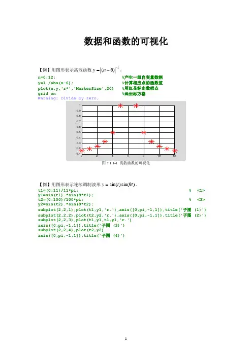
数据和函数的可视化【例】用图形表示离散函数1)6(--=n y 。

n=0:12; %产生一组自变量数据 y=1./abs(n-6); %计算相应点的函数值 plot(n,y,'r*','MarkerSize',20) %用红花标出数据点 grid on %画坐标方格【例】用图形表示连续调制波形)9sin()sin(t t y =。

t1=(0:11)/11*pi; % <1> y1=sin(t1).*sin(9*t1);t2=(0:100)/100*pi; % <3> y2=sin(t2).*sin(9*t2);subplot(2,2,1),plot(t1,y1,'r.'),axis([0,pi,-1,1]),title('子图 (1)') subplot(2,2,2),plot(t2,y2,'r.'),axis([0,pi,-1,1]),title('子图 (2)') subplot(2,2,3),plot(t1,y1,t1,y1,'r.') axis([0,pi,-1,1]),title('子图 (3)') subplot(2,2,4),plot(t2,y2)axis([0,pi,-1,1]),title('子图 (4)')【例】简单例题，比较方便的试验指令。

【例】用图形表示连续调制波形)9sin()sin(t t y 及其包络线。

t=(0:pi/100:pi)'; %长度为101的时间采样列向量 <1> y1=sin(t)*[1,-1]; %包络线函数值，是（101x2）的矩阵 <2> y2=sin(t).*sin(9*t); %长度为101的调制波列向量 <3> t3=pi*(0:9)/9; %<4>y3=sin(t3).*sin(9*t3);plot(t,y1,'r:',t,y2,'b',t3,y3,'bo') % <5> axis([0,pi,-1,1]) %控制轴的范围<6>【例】用复数矩阵形式画利萨如（Lissajous ）图形。