
a r X i v :0705.3182v 1 [a s t r o -p h ] 22 M a y 2007
2Lucio Mayer Alan Boss and Andrew F.Nelson
timescales compared to the accumulation of planetesimals by gravity and the subsequent accretion of gas by a rocky core,the conventional two-stage forma-tion giant planet formation theory known as core accretion(see the chapter by Marzari et al.).
The particular emphasis of this review chapter is on how gravitational instability develops when a protoplanetary disk is not isolated but is a member of a binary or multiple star system(see the chapter by Prato&Weinberger). Indeed such a con?guration is likely to be the most common in the Galaxy: the majority of solar-type stars in the Galaxy belong to double or multiple stellar systems(Duquennoy&Mayor1991;Eggenberger et al.2004).Radial velocity surveys have shown that planets exist in binary or multiple stellar systems where the stars have separations from~20to several thousand AU (Eggenberger et al.2004;see the chapter by Eggenberger&Udry).Although the samples are still small,attempts have been made to compare properties of planets in single and multiple stellar systems(Patience et al.2002;Udry et al.2004).Adaptive optics surveys designed to quantify the relative frequency of planets in single and multiple systems are underway(Udry et al.2004; Chauvin et al.2006).At least30%of extrasolar planetary systems appear to occur in binary or multiple star systems(Raghavan et al.2006).These surveys could o?er a new way to test theories of giant planet formation,provided that di?erent formation models yield di?erent predictions about the e?ects of a stellar companion.
1.1Gravitational instabilities
The parameter that determines whether GIs occur in thin gas disks is
Q=c sκ/πGΣ,(1) where c s is the sound speed,κis the epicyclic frequency at which a?uid element oscillates when perturbed from circular motion,G is the gravitational constant,andΣis the surface density.In a nearly Keplerian disk,κ≈the rotational angular speed?.For axisymmetric(ring-like)disturbances,disks are stable when Q>1(Toomre1964).At high Q-values,pressure,represented by c s in(1),stabilizes short wavelengths,and rotation,represented byκ, stabilizes long wavelengths.The most unstable wavelength when Q<1is given byλm≈2π2GΣ/κ2.
Modern numerical simulations,beginning with Papaloizou&Savonije (1991),show that nonaxisymmetric disturbances,which grow as multi-armed spirals,become unstable for Q<~1.5.Because the instability is both linear and dynamic,small perturbations grow exponentially on the time scale of a rotation period P rot=2π/?.The multi-arm spiral waves that grow have a predominantly trailing pattern,and several modes can appear simultaneously (Boss1998a;Laughlin et al.1997;Nelson et al.1998;Pickett et al.1998).
Numerical simulations show that,as GIs emerge from the linear regime, they may either saturate at nonlinear amplitude or grow enough to fragment
Gravitational instability in binary protoplanetary disks3 the disk.Two major e?ects control or limit the outcome–disk thermody-namics and nonlinear mode coupling.At this point,the disks also develop large surface distortions.As emphasized by Pickett et al.(1998,2000,2003), the vertical structure of the disk plays a crucial role,both for cooling and for essential aspects of the dynamics.As a result,except for isothermal disks,GIs tend to have large amplitudes at the surface of the disk.
Using second and third-order governing equations for spiral modes and comparing their results with a full nonlinear hydrodynamics treatment,Laugh-lin et al.1998studied nonlinear mode coupling in the most detail.Even if only a single mode initially emerges from the linear regime,power is quickly distributed over modes with a wide variety of wavelengths and number of arms,resulting in a self-gravitating turbulence that permeates the disk.In this gravitoturbulence,gravitational torques and even Reynold’s stresses may be important over a wide range of scales(Nelson et al.1998;Gammie2001; Lodato&Rice2004;Mej′?a et al.2005).
As the spiral waves grow,they can steepen into shocks that produce strong localized heating(Pickett et al.1998,2000a;Nelson et al.2000).Gas is also heated by compression and through net mass transport due to gravitational torques.The ultimate source of GI heating is work done by gravity.The subse-quent evolution depends on whether a balance can be reached between heating and the loss of disk thermal energy by radiative or convective cooling.The no-tion of a balance of heating and cooling in the nonlinear regime was described as early as1965by Goldreich&Lynden-Bell and has been used as a basis for proposingα-treatments for GI-active disks(Paczy′n ski1978;Lin&Pringle 1987).For slow to moderate cooling rates,numerical experiments verify that thermal self-regulation of GIs can be achieved(Tomley et al.1991;Pickett et al.1998,2000a,2003;Nelson et al.2000;Gammie2001;Rice et al.2003b; Lodato&Rice2004,2005;Mej′?a et al.2005;Cai et al.2006a,b).Q then hov-ers near the instability limit,and the nonlinear amplitude is controlled by the cooling rate.There have been various attempts to model radiative cooling in self-gravitating disks.For a recent overview of the di?erent methods appear-ing in the literature and for a general discussion of gravitational instability in protoplanetary disks,we point the reader to Durisen et al.(2007).In this chapter we will focus on the radiative cooling models that have been used in the few existing works on binary self-gravitating protoplanetary disks.
1.2Fragmentation and survival of clumps
As shown?rst by Gammie(2001)for local thin-disk calculations and later con?rmed by Rice et al.(2003b)and Mej′?a et al.(2005)in full3D hydro sim-ulations,disks with a?xed cooling time,t cool=U/˙U,fragment for su?ciently fast cooling,speci?cally when t cool≤3??1,or,equivalently,t cool≤P rot/2. Finite thickness has a slight stabilizing in?uence(Rice et al.2003b;Mayer et al.2004a).When dealing with realistic radiative cooling,however,one can-not apply this simple fragmentation criterion to arbitrary initial disk models.
4Lucio Mayer Alan Boss and Andrew F.Nelson
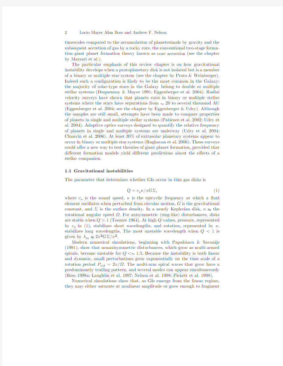
One has to apply it to the asymptotic phase after nonlinear behavior is well-developed(Johnson&Gammie2003).Cooling times can be much longer in the asymptotic state than they are initially(Cai et al.2006a,b;Mej′?a et al.,in preparation).For disks evolved under isothermal conditions,where a simple cooling time cannot be de?ned,local thin-disk calculations show fragmenta-tion when Q<1.4(Johnson&Gammie2003).This is roughly consistent with results from global simulations(e.g.,Boss2000;Nelson et al.1998;Pickett et al.2000a,2003;Mayer et al.2002,2004a).Figure1shows a classic example of a fragmenting disk.
Fig.1.Midplane density contours after339yr of evolution of a0.091M⊙disk in orbit around a single1M⊙protostar,showing the formation of a self-gravitating clump of mass1.4M Jup at4o’clock(Boss2001).
Rice et al.(2003b)also found that clumps could form in disks with even longer cooling times(t cool=5??1)if the disk mass was increased.This latter estimate is in agreement with the time scales for cooling found in3D models with di?usion approximation radiative transfer and convective-like motions that led to fragmentation into self-gravitating clumps(Boss2001,2004a).
Gravitational instability in binary protoplanetary disks5 Although there is general agreement on conditions for fragmentation,two important questions remain.Do real disks ever cool fast enough for fragmen-tation to occur,and do the fragments last long enough to contract into per-manent protoplanets before being disrupted by tidal stresses,shear stresses, physical collisions,and shocks?Recent simulations have just begun to address the issue of the long term survival of clumps once they have been produced in a disk(Durisen et al.2007).None of these long-term simulations has explored the case of binary systems and therefore their results are not necessarily valid in that case(for example they do not take into account the e?ect of even-tual orbital resonances with the companion that might)..However,except for clumps forming at the very periphery of one of the two disks,one would expect the tidal stresses to be dominated by the central star of their own disk,in which case the results of isolated disks are still relevant.In addition, clumps are unlikely to form near the outskirts of disks since the surface den-sity should be too low there.High spatial resolution appears to be crucial for the survival of clumps.Pickett et al.(2003)found that256azimuthal cells were not enough to resolve self-gravity on a scale of a fraction of AU,lead-ing to arti?cial dissolution of overdensities.An increased ability of clumps to persist and become gravitationally bound as the resolution is increased was also found by Boss(2001)and Mayer et al.(2004).High spatial resolution of the gravitational force is crucial,as is the accuracy of a gravity solver for a given resolution element.These features are extremely code-dependent and are brie?y discussed below in section2.2.
2Numerical Techniqes and Assumptions
To date,only three papers have been published that consider the possibility of forming giant planets by disk instability in binary star systems:Nelson (2000),Mayer et al.(2005),and Boss(2006b).In short,Nelson(2000)found that binarity prevented fragmentation from occurring,Boss(2006b)found that binarity could enhance clump formation,and Mayer et al.(2005)found the binarity could discourage fragmentation in some cases,but permit it in other cases.These three papers are the focus of the remainder of this chapter, as we try to decipher the reasons for this apparent dispersion in outcomes.
2.1Hydrodynamics methods
Three codes have been used so far to follow the evolution of binary proto-planetary disks,two smoothed particle hydrodynamics(SPH)codes(Nelson 2000;Mayer et al.2005)and one?nite-di?erence grid-based code(Boss2006b; described in detail by Boss&Myhill1992).The two SPH codes are,respec-tively,a modi?ed version(Nelson2000)of a code originally developed by Benz (1990)and GASOLINE(Wadsley et al.2004;Mayer et al.2005).We begin with a description of the codes.
6Lucio Mayer Alan Boss and Andrew F.Nelson
Although the two SPH codes are based on a very similar implementa-tion of SPH,there are di?erences in some aspects that might be important for understanding di?erences in results.One major di?erence is that the ver-sion of the code used in Nelson(2000)is2D while GASOLINE is3D,as is the Boss(2006b)code.Evidence has been accumulated recently that gravitational instability in a protoplanetary disk is an intrinsically three-dimensional phe-nomenon(Cai et al.2006a,b).At the same time,at the resolution for which a?ordable simulations can be done,3D codes resolve only very poorly the structure of the disk in the third dimension.Nelson(2006)has shown that if the vertical structure is not well resolved,both from a hydrodynamical stand-point and from a radiative transfer standpoint,serious errors in the evolution of the disks may develop.Therefore,even with all other things being equal, this di?erence alone could result in a di?erent evolution of the spiral patterns, and thus of the outcome of gravitational instability.In what follows we will highlight the most important features of the two SPH codes and we will ex-plicitly indicate in what ways the two codes di?er and what is the expected outcome of such di?erences.
SPH is an approach to hydrodynamical modeling?rst developed by Lucy (1976)and Gingold&Monaghan(1977).It is a particle-based method that does not refer to grids for the calculation of hydrodynamical quantities:all forces and?uid properties are determined by moving particles,thereby elimi-nating numerically di?usive advective terms.The Boss&Myhill(1992)code is an Eulerian code,with all quantities de?ned on a spherical coordinate grid. The code is second-order accurate in both space and time,a crucial factor for keeping numerical di?usion at a tolerable level.
The basis of the SPH method is the Lagrangian representation and evo-lution of smoothly varying?uid quantities whose value is only known at disordered discrete points in space occupied by particles.Particles are the fundamental resolution elements comparable to cells in a grid.SPH operates through local summation operations over particles weighted with a smooth-ing kernel,W,that approximates a local integral.The smoothing operation provides a basis from which to obtain derivatives.Thus,estimates of density-related physical quantities and gradients are generated.
Both GASOLINE and Nelson’s code use a fairly standard implementation of the hydrodynamical equations of motion for SPH(Monaghan1992).The density at the location of each particle with index i is calculated from a sum over particle masses m j
ρi=
n
j=1m j W ij.(2)
where j is an index running on the entire set of n particles.The momentum equation is expressed as
Gravitational instability in binary protoplanetary disks7
d v i
ρ2i +
P j
8Lucio Mayer Alan Boss and Andrew F.Nelson
uses reduced moments that require only n+1terms to be stored for the n th moment.For a detailed discussion of the accuracy and e?ciency of the tree algorithm as a function the order of the multipoles used,see Stadel(2001).
Relaxation e?ects compromise the attempt to model continuous?uids us-ing particles.Both in GASOLINE and in Nelson’s code the particle masses are e?ectively smoothed in space using the same spline kernels employed in the SPH calculation.This means that the gravitational forces vanish at zero separation and return to Newtonian1/r2at a separation of?i+?j where?i is the gravitational softening applied to each particle.In this sense the gravi-tational forces are well matched to the SPH forces.However,in GASOLINE gravitational softening is constant over time and?xed at the beginning of the simulation,while in Nelson’s code it is time-dependent and always equal to the local SPH smoothing length.
The use of adaptive softening in Nelson’s code ensures that gravitational and pressure forces are always represented with the same resolution.Bate& Burkert(1997)have shown that when an imbalance between pressure and gravitational forces occurs,arti?cial fragmentation or suppression of physical fragmentation can arise.While Bate&Burkert(1997)found that such im-balance leads to spurious results when it occurs at a scale comparable with the local Jeans length of the system,more recently Nelson(2006)has shown that particle clumping was ampli?ed for imbalances in softening/smoothing even when the Toomre wavelength was well resolved,which is a much more limiting codndition.When the gravitational softening is?xed over time,such as in GASOLINE,care has to be taken that this be comparable to the SPH smoothing length at the scale of the Jeans length.Mayer et al.(2005)choose the softening according to the latter prescription at the beginning of the simu-lation and set its value so that outside10AU the softening drops to~1/2the local smoothing length.An argument can be made that later in the evolution, when strong overdensities develop along the spiral arms the SPH smoothing length drops signi?cantly,becoming smaller than the gravitational softening, thereby degrading the propensity for numerical fragmentation.Both the ini-tial softening/smoothing inequality and the later evolution of disks towards fragmentation were examined by Nelson(2006),with the result that to frag-mentation was still enhanced,but after it began,simulations could be evolved much further,because the fragments did not continue to contract inde?nitely but rather remained comparable in size to the?xed softening value.No spe-ci?c tests of whether this occurs as well in the Mayer et al.work,or how the results may be a?ected,has yet been done.It may be of some note however, that the fragmentation in their work only occured in the outer half of their disks,where the force imbalances favor gravity,as seen in Nelson(2006).
An on going comparison between SPH and adaptive mesh re?nement (AMR)codes conducted at di?erent resolutions and particle softening is in preparation(Mayer et al.,in preparation,see also Durisen et al.2007)and may provide an independent check of the reliability of fragmentation in SPH. On the other hand,since this happens when the gas is optically thick,cooling
Gravitational instability in binary protoplanetary disks9 is also suppressed(see below),and this might be the dominant,physical e?ect in slowing down the collapse.Even so,compensating for insu?ciencies in a physical model,using?aws in a numerical code,would seem to be,at best, undesirable.Adaptive softening is also not without?aws–particles have a time-dependent potential energy,which induces?uctuations in the potential that can in principle increase force errors,possibly a?ecting the accuracy of the integration.This is known to be problematic for purely gravitational simu-lations such as those of cosmic structure formation,but its consequences have not been studied systematically for the case of self-gravitating?uids.Recent work of Price&Monaghan(2006)has shown how adpative softening may be used while still conserving energy,but their technique has not yet seen wide adoption.
In the Boss&Myhill(1992)code,Poisson’s equation is solved for the gravitational potential at each time step.This solution is achieved by using a spherical harmonic(Y lm)expansion of the density and gravitational potential, with terms in the expansion up to l,m=32or48typically being used.Boss (2000,2001)found that the number of terms in this expansion was just as important for robust clump formation as the spatial resolution.Because the computational e?ort involved scales as the number of terms squared,however, in practice this value cannot be increased much beyond48without having the Poisson solver dominate the e?ort.Boss(2005)showed that the introduction of point masses to represent very high density clumps led to better de?ned, more massive clumps,but the computational e?ort associated with introduc-ing these point masses also led to an appreciable slowing the execution speeds.
2.3Timestepping
Nelson’s code uses the Runge-Kutta-Fahlberg method to evolve the equations of motion.It employs a global timestep for all particles in the disk,which was increased or decreased depending on the conditions in the simulations.The integrator is a?rst order accurate method with second order error control and the scheme provides limits on the second order error term in all of the various variables.Gasoline incorporates the timestep scheme described as Kick-Drift-Kick(KDK)(see Wadsley et al.2004).Without gas forces this is a symplectic leap-frog integration,which ensures the conservation of total energy,this being not guaranteed with the Runge-Kutta method(Quinn et al.1997;Tremaine et al.2003),though much better conservation can be had when a single time step for all particles is used,as was done in Nelson(2000).The leap-frog scheme requires only one force evaluation and minimum storage.GASOLINE uses multiple timesteps,hence at any given time di?erent particles in the disk can be evolved with di?erent timesteps.The base(maximum)timestep is divided in a hierarchy of smaller steps(rungs),with di?erent particles being assigned to di?erent rungs.This allows to reach a much smaller step size when it is required,allowing to probe a much higher dynamic range and follow correctly the dynamics of regions with very high densities.The drawback is that the
10Lucio Mayer Alan Boss and Andrew F.Nelson
scheme is no longer strictly symplectic if particles change rungs during the integration which they generally must do to satisfy their individual timestep criteria.Adaptivity in the time integration,hence the ability to achieve small timesteps than the dynamics or hydrodynamics require so,can be important to model correctly the formation and evolution of overdensities and clumps. In fact,if the step size is not small enough the acceleration inside the over-densities,that goes as1/?t2,can be underestimated.This is equivalent to underestimate the self-gravity of clumps and can in principle lead to their arti?cial dissolution,although no systematic tests have ever been performed. GASOLINE uses a standard timestep criterion based on the particle acceler-ation(see Wadsley et al.2004)and for gas particles,the Courant condition and the expansion cooling rate.Nelson’s code adopts the Courant condition as well for hydrodynamical forces and addituonally a set of constraints based on the position and velocities of particles.If the latter are not met after a timestep,the scheme went back and tries again with a smaller timestep.
The Boss&Myhill(1992)code uses a single-size timestep based on the Courant condition,and uses a predictor-corrector method to achieve second-order accuracy in time.
2.4Arti?cial viscosity
Most hydrodynamic methods need arti?cial viscosity to stabilize the?ow by avoiding particle interpenetration and to resolve in an approximate manner the physical dissipation present in shocks,and SPH is no exception.Both Mayer et al.(2005)and Nelson(2000)use bulk and von Neumann-Richtmyer (so called‘ˉα’and‘β’)viscosities to simulate viscous pressures which are linear and quadratic in the velocity divergence.They both incorporate a switch(see Balsara1995)that acts to reduce substantially the large undesirable shear component associated with the standard form.
In both GASOLINE and Nelson’s code the arti?cial viscosity term reads
Πij= ?α11
r2
ij +0.01(h i+h j)2
,(5)
where r ij=r i?r j,v ij=v i?v j,and c j is the sound speed.α=1andβ=2 are standard values of the coe?cients of arti?cial viscosity,known to result in acceptable dissipative behavior across a wide variety of test problems.
In protoplanetary disks,Mach numbers are high(of order10-20)although shocks are not as strong(i.e.the density jumps are not as pronounced)as when gas collapses or collides with other gas along nearly radial trajecto-ries such as in cosmological structure formation.This is important because it
Gravitational instability in binary protoplanetary disks11 means that the standard settings for the viscous coe?cients may be higher than strictly necessary for correct evolution of the?ow.Since arti?cial vis-cosity is essentially a nuisance with regard to improving the modeling of the hydrodynamical?ow,any improvements which decrease the importance of unphysical side e?ects,while retaining the required stability and dissipative e?ects of the code,are desirable.
Mayer et al.(2004)have therefore experimented with lowering the coe?-cients of arti?cial viscosity,?nding that for e.g.α=0.5andβ=0orα=0.5 andβ=1fragmentation is more vigorous.However,the simulations of binary protoplanetary disks in Mayer et al.(2005)were designed following a conser-vative approach,hence the standard valuesα=1andβ=2were employed. They do,however,include a modi?cation due to Balsara(1995),to modify the computation of the velocity divergence from its usual form by multiplying the above equation by a correction factor
|(?·v i)|
f i=
12Lucio Mayer Alan Boss and Andrew F.Nelson
Fig.2.Color coded density maps of two isothermal runs evolved with1million SPH particles.The disk starts with a minimum Toomre parameter approaching Q~1. The snapshots after about8orbital times at10AU,i.e.about240years,are shown. On the left a run without the Balsara correction term is shown,on the right the same disk is evolved with the Balsara term on.
could actually be to enhance the growth and survival of the clumps by taking kinetic energy out of the system.
Arti?cial viscosity,be it explicitly inserted or implicit to the code,is one way in which actual physical processes ocurring on the sub-grid scale,such as shock front heating and dissipation,can be included in the calculation.A tensor formulation arti?cial viscosity is included in the Boss&Myhill(1992) code,but is generally not used in the disk instability models,except to dis-cern the extent to which arti?cial viscosity can suppress fragmentation(Boss 2006b).Numerical stability is maintained instead by using as small a fraction of the Courant time step as is needed,sometimes as low as1%of the Courant value.Boss(2006b)showed that his code reproduced an analytical(Burgers) shock wave solution nearly as well without any arti?cial viscosity as when a standard amount(C Q=1,see Boss&Myhill1992)of arti?cial viscosity was employed,implying that the intrinsic numerical viscosity of his code was su?cient to stabilize such a shock front.Tests on the full set of hydrodynamic equations have not been published.
2.5Internal energy equation
Both GASOLINE and Nelson’s code employ the following energy equation (called“asymmetric”),advocated by Evrard(1990)and Benz(1990),which conserves energy exactly in each pairwise exchange and is dependent only on the local particle pressure,
Gravitational instability in binary protoplanetary disks13
d u i
ρ2i
n
j=1m j v ij·?i W ij,(7)
where u i is the internal energy of particle i,which is equal to1/(γ?1)P i/ρi for an ideal gas.In this formulation entropy is closely conserved making it similar to alternative entropy integration approaches,such as that proposed by Springel&Hernquist(2002).The equation above includes only the part related to P dV work,while the full energy equation has a term due to arti?cial viscosity and one due to cooling to be discussed below.
The adiabatic indexγis di?erent in Nelson(2000)and Mayer et al.(2005) because Nelson(2000)perform only two dimensional simulations,In both cases the value ofγappropriate for a gas at temperatures T<1000K in which rotational transitions are active,but not the vibrational ones,is as-sumed.Because of the di?erences in dimensionality,this assumption yields γ=1.4in3D for the pure hydrogen gas(i.e.average molecular weight of2.0) assumed by Mayer et al.andγ~1.53in2D,for the solar composition gas (average molecular weight2.31)used by Nelson(see also Nelson2006for a discussion of issues that a?ect the ratio of speci?c heats in2D calculations).
A value ofγ=1.42was incorporated into the vertical structure models used in Nelson(2000)in order to remain consistent,since the assumptions implicit in that calculation required a3D treatment.Other published work adopts γ=5/3(Rice et al.2003a,2005;Cai et al.2006a,b).As we explain below, the value ofγcan have an impact on whether fragmentation occurs or not in a self-gravitating disk,both isolated and in a binary system.A recent paper (Boley et al.2006)explains how using just one or two values of the adiabatic independently on the actual temperature and density of the gas is probably a poor approximation of the real physics of molecular hydrogen transitions which can a?ect the outcome of gravitational instability.Future work will need to asess that.
A term dependent on arti?cial viscosity is added to eq.(7)
n
j=1m j1
14Lucio Mayer Alan Boss and Andrew F.Nelson
namic equations are solved.This energy equation includes the e?ects of com-pressional heating and cooling and of radiative transfer,in either the di?usion or Eddington approximations.In the latter case,a separate equation for the mean intensity must be solved.In the di?usion approximation,the energy equation is solved by Boss’s code(Boss2001)in the form
?(ρE)
3κρ
?(σT4)
whereρ=gas density,v=?uid velocity,E=speci?c internal energy= E(ρ,T),p=gas pressure=p(ρ,T),κ=Rosseland mean opacity of gas and dust=κ(ρ,T),T=gas and dust temperature,andσ=Stefan-Boltzmann constant=5.67×10?5cgs.The di?usion approximation energy equation has been used for all of Boss’s disk instability models with radiative transfer to date.However,the Eddington approximation energy equation was used to derive the initial quasi-steady state thermal pro?les(Boss1996)used for the initial conditions in Boss’s disk instability models.In the Eddington approx-imation code,the energy equation is
?(ρE)
3?·(
1
31
κρ
?J)?J=?B
The computational burden associated with the iterative solution of the mean intensity equation in the Eddington approximation has so far precluded its use in disk instability models with the high spatial resolution needed to follow the evolution over many orbital periods.Because of the high optical depths at the midplane(up toτ~104)of these disks,however,the di?usion approximation is valid near the critical disk midplane,and radiative transfer in the di?usion approximation imposes little added computational burden.
Gravitational instability in binary protoplanetary disks15 2.6Cooling in the simulations
Nelson et al.(2000)and Nelson(2000)requires that the disk be in instanta-neous vertical entropy equilibrium and instantaneous vertical thermal balance in order to determine its structure.This implicitly assumes that the disk will be convectively unstable vertically over a short timescale and quickly restore thermal balance.Convection is expected given the high optical depths of mas-sive gravitationally unstable disks(Ruden&Pollack1996);vigorous vertical currents with features resemblant of convective instabilities have been indeed observed in massive protoplanetary disks modeled with either SPH and grid codes(Boss2003,2004;Mayer et al.2006).Under these assumptions the gas is locally(and instantaneously)adiabatic as a function of z.In an adiabatic medium,the gas pressure and density are related by p=Kργand the heat capacity of the gas,C V,is a constant(by extension,also the ratio of speci?c heats,γ,see above).In fact,this will not be the case in general because,in various temperature regimes,molecular hydrogen will have active rotational or vibrational modes,it may dissociate into atomic form or it may become ionized.
From the now known(ρ,T)structure,Nelson et al.derive the temperature of the disk photosphere by a numerical integration of the optical depth,τ,from z=∞to the altitude at which the optical depth becomesτ=2/3
τ=2/3= z phot∞ρ(z)κ(ρ,T)dz.(9) In optically thin regions,for whichτ<2/3at the midplane,they assume the photosphere temperature is that of the midplane.The photosphere tem-perature is then tabulated as a function of the three input variables radius, surface density and speci?c internal energy.At each time the photosphere temperature is determined for each particle from such table and used to cool the particle as a blackbody at that temperature.The cooling of any particular particle proceeds as
du i
(10)
Σj
whereσR is the Stefan-Boltzmann constant,u i andΣi are the speci?c internal energy and surface density of particle i and T eff is its photospheric temperature.The factor of two accounts for the two surfaces of the disk.On every particle,the condition that the temperature(both midplane and photo-sphere)never falls below the3K cosmic background temperature is enfoced. Rosseland mean opacities from tables of Pollack,McKay&Christo?erson (1985)are used.Opacities for packets of matter above the grain destruction temperature are taken from Alexander&Ferguson(1994).
In parts of the disk where the calculated midplane temperature is greater than dust vaporization temperature,the opacity is temporarily reduced to ~5%of its tabulated values over the entire column above and below that
16Lucio Mayer Alan Boss and Andrew F.Nelson
point in the disk.This accounts for the fact that dust formation,after once being vaporized,may occur at rates slower than the timescales for vertical transport through the column.In other regions of the disk we assume that the opacity remains una?ected.
Cooling is treated very di?erently in Mayer et al.(2005).Cooling is in-dependent on distance from the midplane also in this case(so there is no dependence on z,as if there was constant thermal equilibrium vertically)but there is an explicit dependence on the distance from the center.The cooling term is proportional to the local orbital time,t orb=2π/?,where?is the angular velocity,via the following equation
Λ=dU/dt=U/A??1(11) The disk orbital time is a natural characteristic timescale for spiral modes developing in a rotating disk.Cooling is switched o?inside5AU in order to maintain temperatures high enough to be comparable to those in protosolar nebula models(e.g.Boss1998),and in regions reaching a density above10?10 g/cm3to account for the local high optical depth;indeed according to the sim-ulations of Boss(2002)with?ux-limited di?usion the temperature of the gas evolves nearly adiabatically above such densities.In practice in these regions the gas simply obeys eq.(7)with the arti?cial viscosity term(8).Mayer et al. (2005)considered cooling times going from0.3to1.5the local orbital time. The jury is still out on whether the cooling times adopted here are credible or excessively short.Recent calculations by Boss(2002,2004),Johnson&Gam-mie(2003)and Mayer et al.(2006),which use di?erent approximate treat-ments of radiative transfer,do?nd cooling times of this magnitude through a combination of radiative losses and convection,but other works such as those of Mejia et al.(2005),Cai et al.(2006)and Boley et al.(2006)encounter longer cooling times and never?nd fragmentation.The cooling times used in Nelson(2000)are about25times longer than the typical orbital time in the region(5?10AU),hence they were much longer than in Mayer et al.(2005). As we shall see,this will have profound implications on the?nal outcome of the simulations.
In work in progress,one of the authors,L.Mayer,has begun performing simulations of binary protoplanetary disks using the new?ux-limited di?u-sion scheme for radiative transfer adopted in Mayer et al.(2006),which adopts the?ux-limiter of Bodenheimer et al.(1991)in the transition between opti-cally thick and optically thin regions of the disk.The disk then radiates as a blackbody at the edge,with the radiative e?ciency being modulated by a pa-rameter that de?nes how large is the emitting surface area,or in other words, the part of the disk that quali?es as edge.In section5we brie?y describe some preliminary results of these new calculations.
Boss(2001)noted that in his di?usion approximation models,the radiative ?ux term is set equal to zero in regions where the optical depthτdrops below 10,so that the di?usion approximation does not a?ect the solution in low
Gravitational instability in binary protoplanetary disks17 optical depth regions where it is not valid.This assumption is intended to err on the conservative side of limiting radiative cooling.A test model(Boss 2001)that varied this assumption by using a criticalτc=1instead of10 led to essentially the same results as withτc=10,implying insensitivity of the results to this assumption.Another test model(Boss2001)used a more detailed?ux-limiter to ensure that the radiative energy?ux did not exceed the speed of light(speci?cally,that the magnitude of the net?ux vector H did not exceed the mean intensity J),and also yielded essentially the same results as the model with the standard assumptions.In low optical depth regions such as the disk envelope,the gas and dust temperature is assumed to be50K.
In the Boss(2006b)models,the disk was assumed to be embedded in an infalling envelope of gas and dust that formed a thermal bath with a temperature of50K.Thus the e?ective surface boundary condition on the disk is50K.Boss(2004a)found that convective-like motions occurred in the models with a vigor su?cient to transport the heat produced at the midplane by clump formation to the surface of the disk,where it is e?ectively assumed to be radiated away into the protostellar envelope.This code also employs a full thermodynamical description of the gas,including detailed equations of state for the gas pressure,the speci?c internal energy,and the dust grain and atomic opacities in the Rosseland mean approximation.
Molecular hydrogen dissociation is treated,as well as a parameterized treatment of the transition between para-and ortho-hydrogen.Linear inter-polation from100K to200K is used to represent the variations between a speci?c internal energy per gram of hydrogen of3/2R g T/μ(where R g is the gas constant,T is the temperature,andμ=2is the mean molecular weight for molecular hydrogen)for temperatures less than100K and of5/2R g T/μfor temperatures above200K.No discontinuities are present in this internal energy equation of state,which has been used in all of Boss’s disk instability models.
Ra?kov(2006)has noted that while vigorous convection is possible in disks,the disk photosphere will limit the disk’s radiative losses and so may control the outcome of a disk instability.Numerical experiments designed to further test the radiative transfer treatment employed in the Boss models (beyond the tests described above)have been completed,and other models are underway(Boss2007,in preparation).Understanding the extent to which the surface of a fully3D disk,with optical depths that vary in all directions and with corrugations that may shield the disk’s surface from the central protostar and other regions of the disk,requires a fully numerical treatment and is not amenable to a simple analytical approach.
18Lucio Mayer Alan Boss and Andrew F.Nelson
3Initial and Boundary Conditions
Here we describe the initial and boundary conditions for the models,focusing on the di?erent choices made by di?erent workers.These choices include(1) density and temperature pro?les of the disks,(2)disk masses and Toomre parameters,(3)spatial resolution,(4)the boundary conditions,and(5)the orbital con?guration in the binary experiments.
One important di?erence to point out is that Mayer et al.(2005)start their binary simulations after growing the individual disks in isolation.The disk mass is grown until it reaches the desired value while keeping the temperature of the particles constant over time.The Toomre parameter is prevented from falling below2by setting the temperature of the disk su?ciently high at the start.This way the initial conditions used for the binary experiments are those of a gravitationally stable disk.The Toomre parameter is then lowered to a value in the range1.4?2by resetting the temperature of the particles before placing the disk on the binary orbit(the temperature is set to65K,hence the Toomre parameter will depend on the mass of the disk,see below in the next two sections).As the disk evolves in isolation,it expands slightly,losing the sharp outer edges.The inner hole also?lls up partially,but most of the particles remain on very similar orbits.Once the disk is placed on an orbit around a companion disk,the system is further evolved using the full energy equation plus a cooling term dependent on the orbital time,therefore including adiabatic compression and expansion,irreversible shock heating and radiative cooling.Nelson(2000)do not grow the disk but start with a treatment that also solves the full energy equation but treats the cooling term di?erently(see above).
In both Mayer et al.(2005)and Nelson(2000)matter is set up on initially circular orbits assuming rotational equilibrium in the disk.The central star is modeled by a single massive,softened particle.Radial velocities are set to zero. Gravitational and pressure forces are balanced by centrifugal forces including the small contribution of the disk mass.The magnitudes of the pressure and self-gravitational forces are small compared to the stellar term,therefore the disk is nearly Keplerian in character.No explicit initial perturbations are as-sumed beyond computational roundo?error in either Mayer et al.(2005)or Nelson(2000).Due to the discrete representation of the?uid variables,this perturbation translates to a noise level of order~10?3?10?2for the SPH calculations.The relatively large amplitude of the noise originates from the fact that the hydrodynamic quantities are smoothed using a comparatively small number of neighbors(see Herant&Woosley1994).An increase in the number of particles does not necessarily decrease the noise unless the smooth-ing extends over a larger number of neighbors.This perturbation provides the initial seed that can be ampli?ed by gravitational instability.The initial disk model in Boss(2006b)is rotating with a near-Keplerian angular velocity chosen to maximize the stability of the initial equilibrium state,with zero translational motions.The envelope above the disk,however,is assumed to
Gravitational instability in binary protoplanetary disks19 be falling down with free-fall velocities but with the same angular velocity pro?le as the rotating disk.Random cell-to-cell noise at the level of10%is introduced to the disk density to seed the cloud with non-axisymmetry at a controlled level.
3.1Density and temperature pro?les
Mayer et al.(2005)grow the disks slowly over time until the desired mass is reached.The initial disk models extend from4to20AU and have a surface density pro?leΣ(r)~r?1.5with an exponential cut-o?at both the inner and outer edge.The initial vertical density structure of the disks is imposed by assuming hydrostatic equilibrium for an assumed temperature pro?le T(r). Nelson(2000)adopts a power law for the initial disk surface density pro?le of the form
Σ(r)=Σ0 1+ r2,(12)
where p is3/2andΣ0is the central surface density of the disk,which is de-termined once the total disk mass is assigned.The Nelson(2000)disk extends from0.3to15AU,and the core radius used for the power laws to the value r c=1AU.The stars had Plummer softening of0.2AU each,while a soften-ing length of2AU was used with the spline kernel softening in Mayer et al. (2005).
The shape of the initial temperature pro?le in Mayer et al.(2005)is similar to that used by Boss(1998,2001)and is shown in Figure3together with the pro?les of several runs with either binary or isolated disks after a few orbits of evolution.
The temperature depends only on radius,so there is no di?erence between midplane and an atmosphere.Between5and10AU the temperature varies as~r?1/2,which resembles the slope obtained if viscous accretion onto the central star is the key driver of disk evolution(Boss1993).Between4and 5AU the temperature pro?le rises more steeply,in agreement with the2D radiative transfer calculations of Boss(1996),while it smoothly?attens out for R>10AU and reaches a constant minimum temperature(an exponential cut-o?is used).The initial temperature pro?le of Nelson(2000)is instead
T(r)=T0 1+ r2,(13)
where q is1/2and T0is the central temperature,which is determined once the minimum desired Toomre parameter,and hence the minimum temperature, is determined(see above).
In Mayer et al.(2005)the minimum temperature is?xed to65K.It is implicitly assumed that the disk temperature is related to the temperature of
20Lucio Mayer Alan Boss and Andrew F.Nelson
Fig.3.Azimuthally averaged mid-plane temperature pro?les at the time of maxi-mum amplitude of the overdensities(at between120years and2000years of evolu-tion depending on the model)in some of the runs described in Mayer et al.(2005). The initial temperature pro?le is shown by the thick solid line.We show the results for a run with two massive disks(M=0.1M⊙,thick short-dashed line,the disks do not fragment)at a separation of about60AU,a run with just one of these two disks in isolation(thin long-dashed line,disk fragments),a run with the same massive disks at a larger separation of116AU(disks fragment)and a run with two light disks(M=0.01M⊙,the disks do not fragment)at a separation of60AU.The runs adopt cooling times in the range0.5?1.5the local orbital time.A smaller separation and a larger disk mass both favour stronger spiral shocks and hence a larger temperature increase during the evolution.
the embedding molecular cloud core from which the disk would be accreting material(Boss1996).Note that,at least for the protosolar nebula,50K is probably a conservative upper limit for the characteristic temperature at R>10AU based on the chemical composition of comets in the Solar System (temperatures as low as20K are suggested in the recent study by Kawakita et al.2001).Outer temperatures between30and70K are found also for several T Tauri disks by modeling their spectral energy distribution assuming a mixture of gas and dust and including radiative transfer(D’Alessio et al. 2001).
In the Boss(2006b)models,the initial disk is an approximate semi-analytic equilibrium model(Boss1993)with a temperature pro?le derived from the Eddingtion approximation radiative transfer models of Boss(1996).The outer disk temperatures were taken to be either40K,50K,60K,70K,or80K,in order to test the e?ects of starting with disks that were either marginally grav-itationally unstable(40K,50K)or gravitationally stable(60K,70K,80K).The
常用整流二极管 型号VRM/Io IFSM/ VF /Ir 封装用途说明1A5 600V/1.0A 25A/1.1V/5uA[T25] D2.6X3.2d0.65 1A6 800V/1.0A 25A/1.1V/5uA[T25] D2.6X3.2d0.65 6A8 800V/6.0A 400A/1.1V/10uA[T60] D9.1X9.1d1.3 1N4002 100V/1.0A 30A/1.1V/5uA[T75] D2.7X5.2d0.9 1N4004 400V/1.0A 30A/1.1V/5uA[T75] D2.7X5.2d0.9 1N4006 800V/1.0A 30A/1.1V/5uA[T75] D2.7X5.2d0.9 1N4007 1000V/1.0A 30A/1.1V/5uA[T75] D2.7X5.2d0.9 1N5398 800V/1.5A 50A/1.4V/5uA[T70] D3.6X7.6d0.9 1N5399 1000V/1.5A 50A/1.4V/5uA[T70] D3.6X7.6d0.9 1N5402 200V/3.0A 200A/1.1V/5uA[T105] D5.6X9.5d1.3 1N5406 600V/3.0A 200A/1.1V/5uA[T105] D5.6X9.5d1.3 1N5407 800V/3.0A 200A/1.1V/5uA[T105] D5.6X9.5d1.3 1N5408 1000V/3.0A 200A/1.1V/5uA[T105] D5.6X9.5d1.3 RL153 200V/1.5A 60A/1.1V/5uA[T75] D3.6X7.6d0.9 RL155 600V/1.5A 60A/1.1V/5uA[T75] D3.6X7.6d0.9 RL156 800V/1.5A 60A/1.1V/5uA[T75] D3.6X7.6d0.9 RL203 200V/2.0A 70A/1.1V/5uA[T75] D3.6X7.6d0.9 RL205 600V/2.0A 70A/1.1V/5uA[T75] D3.6X7.6d0.9 RL206 800V/2.0A 70A/1.1V/5uA[T75] D3.6X7.6d0.9 RL207 1000V/2.0A 70A/1.1V/5uA[T75] D3.6X7.6d0.9 RM11C 1000V/1.2A 100A/0.92V/10uA D4.0X7.2d0.78 MR750 50V/6.0A 400A/1.25V/25uA D8.7x6.3d1.35 MR751 100V/6.0A 400A/1.25V/25uA D8.7x6.3d1.35 MR752 200V/6.0A 400A/1.25V/25uA D8.7x6.3d1.35 MR754 400V/6.0A 400A/1.25V/25uA D8.7x6.3d1.35 MR756 600V/6.0A 400A/1.25V/25uA D8.7x6.3d1.35 MR760 1000V/6.0A 400A/1.25V/25uA D8.7x6.3d1.35 常用整流二极管(全桥) 型号VRM/Io IFSM/ VF /Ir 封装用途说明RBV-406 600V/*4A 80A/1.10V/10uA 25X15X3.6 RBV-606 600V/*6A 150A/1.05V/10uA 30X20X3.6 RBV-1306 600V/*13A 80A/1.20V/10uA 30X20X3.6 RBV-1506 600V/*15A 200A/1.05V/50uA 30X20X3.6 RBV-2506 600V/*25A 350A/1.05V/50uA 30X20X3.6 常用肖特基整流二极管SBD 型号VRM/Io IFSM/ VF Trr1/Trr2 封装用途说明EK06 60V/0.7A 10A/0.62V 100nS D2.7X5.0d0.6 SK/高速 EK14 40V/1.5A 40A/0.55V 200nS D4.0X7.2d0.78 SK/低速 D3S6M 60V/3.0A 80A/0.58V 130p SB340 40V/3.0A 80A/0.74V 180p SB360 60V/3.0A 80A/0.74V 180p SR260 60V/2.0A 50A/0.70V 170p MBR1645 45V/16A 150A/0.65V <10nS TO220 超高速
常用二极管参数 2008-10-22 11:48 05Z6.2Y 硅稳压二极管 Vz=6~6.35V, Pzm=500mW, 05Z7.5Y 硅稳压二极管 Vz=7.34~7.70V, Pzm=500mW, 05Z13X 硅稳压二极管 Vz=12.4~13.1V, Pzm=500mW, 05Z15Y 硅稳压二极管 Vz=14.4~15.15V, Pzm=500mW, 05Z18Y 硅稳压二极管 Vz=17.55~18.45V, Pzm=500mW, 1N4001 硅整流二极管 50V, 1A,(Ir=5uA, Vf=1V, Ifs=50A) 1N4002 硅整流二极管 100V, 1A, 1N4003 硅整流二极管 200V, 1A, 1N4004 硅整流二极管 400V, 1A, 1N4005 硅整流二极管 600V, 1A, 1N4006 硅整流二极管 800V, 1A, 1N4007 硅整流二极管 1000V, 1A, 1N4148 二极管 75V, 4PF, Ir=25nA, Vf=1V, 1N5391 硅整流二极管 50V, 1.5A,(Ir=10uA, Vf=1.4V, Ifs=50A) 1N5392 硅整流二极管 100V, 1.5A, 1N5393 硅整流二极管 200V, 1.5A, 1N5394 硅整流二极管 300V, 1.5A, 1N5395 硅整流二极管 400V, 1.5A, 1N5396 硅整流二极管 500V, 1.5A, 1N5397 硅整流二极管 600V, 1.5A, 1N5398 硅整流二极管 800V, 1.5A, 1N5399 硅整流二极管 1000V, 1.5A, 1N5400 硅整流二极管 50V, 3A,(Ir=5uA, Vf=1V, Ifs=150A) 1N5401 硅整流二极管 100V, 3A, 1N5402 硅整流二极管 200V, 3A, 1N5403 硅整流二极管 300V, 3A, 1N5404 硅整流二极管 400V, 3A, 1N5405 硅整流二极管 500V, 3A, 1N5406 硅整流二极管 600V, 3A, 1N5407 硅整流二极管 800V, 3A, 1N5408 硅整流二极管 1000V, 3A, 1S1553 硅开关二极管 70V, 100mA, 300mW, 3.5PF, 300ma, 1S1554 硅开关二极管 55V, 100mA, 300mW, 3.5PF, 300ma, 1S1555 硅开关二极管 35V, 100mA, 300mW, 3.5PF, 300ma, 1S2076 硅开关二极管 35V, 150mA, 250mW, 8nS, 3PF, 450ma, Ir≤1uA, Vf≤0.8V,≤1.8PF, 1S2076A 硅开关二极管 70V, 150mA, 250mW, 8nS, 3PF, 450ma, 60V, Ir≤1uA, Vf≤0.8V,≤1.8PF, 1S2471 硅开关二极管80V, Ir≤0.5uA, Vf≤1.2V,≤2PF, 1S2471B 硅开关二极管 90V, 150mA, 250mW, 3nS, 3PF, 450ma, 1S2471V 硅开关二极管 90V, 130mA, 300mW, 4nS, 2PF, 400ma, 1S2472 硅开关二极管50V, Ir≤0.5uA, Vf≤1.2V,≤2PF, 1S2473 硅开关二极管35V, Ir≤0.5uA, Vf≤1.2V,≤3PF,
1.塑封整流二极管 序号型号IF VRRM VF Trr 外形 A V V μs 1 1A1-1A7 1A 50-1000V 1.1 R-1 2 1N4001-1N4007 1A 50-1000V 1.1 DO-41 3 1N5391-1N5399 1.5A 50-1000V 1.1 DO-15 4 2A01-2A07 2A 50-1000V 1.0 DO-15 5 1N5400-1N5408 3A 50-1000V 0.95 DO-201AD 6 6A05-6A10 6A 50-1000V 0.95 R-6 7 TS750-TS758 6A 50-800V 1.25 R-6 8 RL10-RL60 1A-6A 50-1000V 1.0 9 2CZ81-2CZ87 0.05A-3A 50-1000V 1.0 DO-41 10 2CP21-2CP29 0.3A 100-1000V 1.0 DO-41 11 2DZ14-2DZ15 0.5A-1A 200-1000V 1.0 DO-41 12 2DP3-2DP5 0.3A-1A 200-1000V 1.0 DO-41 13 BYW27 1A 200-1300V 1.0 DO-41 14 DR202-DR210 2A 200-1000V 1.0 DO-15 15 BY251-BY254 3A 200-800V 1.1 DO-201AD 16 BY550-200~1000 5A 200-1000V 1.1 R-5 17 PX10A02-PX10A13 10A 200-1300V 1.1 PX 18 PX12A02-PX12A13 12A 200-1300V 1.1 PX 19 PX15A02-PX15A13 15A 200-1300V 1.1 PX 20 ERA15-02~13 1A 200-1300V 1.0 R-1 21 ERB12-02~13 1A 200-1300V 1.0 DO-15 22 ERC05-02~13 1.2A 200-1300V 1.0 DO-15 23 ERC04-02~13 1.5A 200-1300V 1.0 DO-15 24 ERD03-02~13 3A 200-1300V 1.0 DO-201AD 25 EM1-EM2 1A-1.2A 200-1000V 0.97 DO-15 26 RM1Z-RM1C 1A 200-1000V 0.95 DO-15 27 RM2Z-RM2C 1.2A 200-1000V 0.95 DO-15 28 RM11Z-RM11C 1.5A 200-1000V 0.95 DO-15 29 RM3Z-RM3C 2.5A 200-1000V 0.97 DO-201AD 30 RM4Z-RM4C 3A 200-1000V 0.97 DO-201AD 2.快恢复塑封整流二极管 序号型号IF VRRM VF Trr 外形 A V V μs (1)快恢复塑封整流二极管 1 1F1-1F7 1A 50-1000V 1.3 0.15-0.5 R-1 2 FR10-FR60 1A-6A 50-1000V 1. 3 0.15-0.5 3 1N4933-1N4937 1A 50-600V 1.2 0.2 DO-41 4 1N4942-1N4948 1A 200-1000V 1.3 0.15-0. 5 DO-41 5 BA157-BA159 1A 400-1000V 1.3 0.15-0.25 DO-41 6 MR850-MR858 3A 100-800V 1.3 0.2 DO-201AD
常用稳压管型号对照——(朋友发的) 美标稳压二极管型号 1N4727 3V0 1N4728 3V3 1N4729 3V6 1N4730 3V9 1N4731 4V3 1N4732 4V7 1N4733 5V1 1N4734 5V6 1N4735 6V2 1N4736 6V8 1N4737 7V5 1N4738 8V2 1N4739 9V1 1N4740 10V 1N4741 11V 1N4742 12V 1N4743 13V 1N4744 15V 1N4745 16V 1N4746 18V 1N4747 20V 1N4748 22V 1N4749 24V 1N4750 27V 1N4751 30V 1N4752 33V 1N4753 36V 1N4754 39V 1N4755 43V 1N4756 47V 1N4757 51V 需要规格书请到以下地址下载, 经常看到很多板子上有M记的铁壳封装的稳压管,都是以美标的1N系列型号标识的,没有具体的电压值,刚才翻手册查了以下3V至51V的型号与电压的对 照值,希望对大家有用 1N4727 3V0 1N4728 3V3 1N4729 3V6 1N4730 3V9
1N4733 5V1 1N4734 5V6 1N4735 6V2 1N4736 6V8 1N4737 7V5 1N4738 8V2 1N4739 9V1 1N4740 10V 1N4741 11V 1N4742 12V 1N4743 13V 1N4744 15V 1N4745 16V 1N4746 18V 1N4747 20V 1N4748 22V 1N4749 24V 1N4750 27V 1N4751 30V 1N4752 33V 1N4753 36V 1N4754 39V 1N4755 43V 1N4756 47V 1N4757 51V DZ是稳压管的电器编号,是和1N4148和相近的,其实1N4148就是一个0.6V的稳压管,下面是稳压管上的编号对应的稳压值,有些小的稳压管也会在管体 上直接标稳压电压,如5V6就是5.6V的稳压管。 1N4728A 3.3 1N4729A 3.6 1N4730A 3.9 1N4731A 4.3 1N4732A 4.7 1N4733A 5.1 1N4734A 5.6 1N4735A 6.2 1N4736A 6.8 1N4737A 7.5 1N4738A 8.2 1N4739A 9.1 1N4740A 10 1N4741A 11 1N4742A 12 1N4743A 13
二极管封装大全 篇一:贴片二极管型号、参数 贴片二极管型号.参数查询 1、肖特基二极管SMA(DO214AC) 2010-2-2 16:39:35 标准封装: SMA 2010 SMB 2114 SMC 3220 SOD123 1206 SOD323 0805 SOD523 0603 IN4001的封装是1812 IN4148的封装是1206 篇二:常见贴片二极管三极管的封装 常见贴片二极管/三极管的封装 常见贴片二极管/三极管的封装 二极管: 名称尺寸及焊盘间距其他尺寸相近的封装名称 SMC SMB SMA SOD-106 SC-77A SC-76/SC-90A SC-79 三极管: LDPAK
DPAK SC-63 SOT-223 SC-73 TO-243/SC-62/UPAK/MPT3 SC-59A/SOT-346/MPAK/SMT3 SOT-323 SC-70/CMPAK/UMT3 SOT-523 SC-75A/EMT3 SOT-623 SC-89/MFPAK SOT-723 SOT-923 VMT3 篇三:常用二极管的识别及ic封装技术 常用晶体二极管的识别 晶体二极管在电路中常用“D”加数字表示,如: D5表示编号为5的二极管。 1、作用:二极管的主要特性是单向导电性,也就是在正向电压的作用下,导通电阻很小;而在反向电压作用下导通电阻极大或无穷大。正因为二极管具有上述特性,无绳电话机中常把它用在整流、隔离、稳压、极性保护、编码控制、调频调制和静噪等电路中。 电话机里使用的晶体二极管按作用可分为:整流二极管(如1N4004)、隔离二极管(如1N4148)、肖特基二极管(如BAT85)、发光二极管、稳压二极管等。 2、识别方法:二极管的识别很简单,小功率二极管的N极(负极),在二极管外表大多采用一种色圈标出来,有些二极管也用二极管专用符号来表示P极(正极)或N极(负极),也有采用符号标志为“P”、“N”来确定二极管极性的。发光二极管的正负极可从引脚长短来识别,长
1N 系列常用整流二极管的主要参数
反向工作 峰值电压 URM/V 额定正向 整流电流 整流电流 IF/A 正向不重 复浪涌峰 值电流 IFSM/A 正向 压降 UF/V 反向 电流 IR/uA 工作 频率 f/KHZ 外形 封装
型 号
1N4000 1N4001 1N4002 1N4003 1N4004 1N4005 1N4006 1N4007 1N5100 1N5101 1N5102 1N5103 1N5104 1N5105 1N5106 1N5107 1N5108 1N5200 1N5201 1N5202 1N5203 1N5204 1N5205 1N5206 1N5207 1N5208 1N5400 1N5401 1N5402 1N5403 1N5404 1N5405 1N5406 1N5407 1N5408
25 50 100 200 400 600 800 1000 50 100 200 300 400 500 600 800 1000 50 100 200 300 400 500 600 800 1000 50 100 200 300 400 500 600 800 1000
1
30
≤1
<5
3
DO-41
1.5
75
≤1
<5
3
DO-15
2
100
≤1
<10
3
3
150
≤0.8
<10
3
DO-27
常用二极管参数: 05Z6.2Y 硅稳压二极管 Vz=6~6.35V,Pzm=500mW,
1N系列稳压管
快恢复整流二极管
常用整流二极管型号和参数 05Z6.2Y 硅稳压二极管 Vz=6~6.35V,Pzm=500mW, 05Z7.5Y 硅稳压二极管 Vz=7.34~7.70V,Pzm=500mW, 05Z13X硅稳压二极管 Vz=12.4~13.1V,Pzm=500mW, 05Z15Y硅稳压二极管 Vz=14.4~15.15V,Pzm=500mW, 05Z18Y硅稳压二极管 Vz=17.55~18.45V,Pzm=500mW, 1N4001硅整流二极管 50V, 1A,(Ir=5uA,Vf=1V,Ifs=50A) 1N4002硅整流二极管 100V, 1A, 1N4003硅整流二极管 200V, 1A, 1N4004硅整流二极管 400V, 1A, 1N4005硅整流二极管 600V, 1A, 1N4006硅整流二极管 800V, 1A, 1N4007硅整流二极管 1000V, 1A, 1N4148二极管 75V, 4PF,Ir=25nA,Vf=1V, 1N5391硅整流二极管 50V, 1.5A,(Ir=10uA,Vf=1.4V,Ifs=50A) 1N5392硅整流二极管 100V,1.5A, 1N5393硅整流二极管 200V,1.5A, 1N5394硅整流二极管 300V,1.5A, 1N5395硅整流二极管 400V,1.5A, 1N5396硅整流二极管 500V,1.5A, 1N5397硅整流二极管 600V,1.5A, 1N5398硅整流二极管 800V,1.5A, 1N5399硅整流二极管 1000V,1.5A, 1N5400硅整流二极管 50V, 3A,(Ir=5uA,Vf=1V,Ifs=150A) 1N5401硅整流二极管 100V,3A, 1N5402硅整流二极管 200V,3A, 1N5403硅整流二极管 300V,3A, 1N5404硅整流二极管 400V,3A,
常用稳压二极管技术参数及老型号代换 型号最大功耗 (mW) 稳定电压(V) 电流(mA) 代换型号国产稳压管日立稳压管 HZ4B2 500 3.8 4.0 5 2CW102 2CW21 4B2 HZ4C1 500 4.0 4.2 5 2CW102 2CW21 4C1 HZ6 500 5.5 5.8 5 2CW103 2CW21A 6B1 HZ6A 500 5.2 5.7 5 2CW103 2CW21A HZ6C3 500 6 6.4 5 2CW104 2CW21B 6C3 HZ7 500 6.9 7.2 5 2CW105 2CW21C HZ7A 500 6.3 6.9 5 2CW105 2CW21C HZ7B 500 6.7 7.3 5 2CW105 2CW21C HZ9A 500 7.7 8.5 5 2CW106 2CW21D HZ9CTA 500 8.9 9.7 5 2CW107 2CW21E HZ11 500 9.5 11.9 5 2CW109 2CW21G HZ12 500 11.6 14.3 5 2CW111 2CW21H HZ12B 500 12.4 13.4 5 2CW111 2CW21H HZ12B2 500 12.6 13.1 5 2CW111 2CW21H 12B2 HZ18Y 500 16.5 18.5 5 2CW113 2CW21J HZ20-1 500 18.86 19.44 2 2CW114 2CW21K HZ27 500 27.2 28.6 2 2CW117 2CW21L 27-3 HZT33-02 400 31 33.5 5 2CW119 2CW21M RD2.0E(B) 500 1.88 2.12 20 2CW100 2CW21P 2B1 RD2.7E 400 2.5 2.93 20 2CW101 2CW21S RD3.9EL1 500 3.7 4 20 2CW102 2CW21 4B2 RD5.6EN1 500 5.2 5.5 20 2CW103 2CW21A 6A1 RD5.6EN3 500 5.6 5.9 20 2CW104 2CW21B 6B2 RD5.6EL2 500 5.5 5.7 20 2CW103 2CW21A 6B1 RD6.2E(B) 500 5.88 6.6 20 2CW104 2CW21B RD7.5E(B) 500 7.0 7.9 20 2CW105 2CW21C RD10EN3 500 9.7 10.0 20 2CW108 2CW21F 11A2 RD11E(B) 500 10.1 11.8 15 2CW109 2CW21G RD12E 500 11.74 12.35 10 2CW110 2CW21H 12A1 RD12F 1000 11.19 11.77 20 2CW109 2CW21G RD13EN1 500 12 12.7 10 2CW110 2CW21H 12A3 RD15EL2 500 13.8 14.6 15 2CW112 2CW21J 12C3 RD24E 400 22 25 10 2CW116 2CW21H 24-1
常用稳压管型号参数对照 3V到51V 1W稳压管型号对照表1N4727 3V0 1N4728 3V3 1N4729 3V6 1N4730 3V9 1N4731 4V3 1N4732 4V7 1N4733 5V1 1N4734 5V6 1N4735 6V2 1N4736 6V8 1N4737 7V5
1N4739 9V1 1N4740 10V 1N4741 11V 1N4742 12V 1N4743 13V 1N4744 15V 1N4745 16V 1N4746 18V 1N4747 20V 1N4748 22V 1N4749 24V 1N4750 27V 1N4751 30V
1N4753 36V 1N4754 39V 1N4755 43V 1N4756 47V 1N4757 51V 摩托罗拉IN47系列1W稳压管IN4728 3.3v IN4729 3.6v IN4730 3.9v IN4731 4.3 IN4732 4.7 IN4733 5.1
IN4735 6.2 IN4736 6.8 IN4737 7.5 IN4738 8.2 IN4739 9.1 IN4740 10 IN4741 11 IN4742 12 IN4743 13 IN4744 15 IN4745 16 IN4746 18 IN4747 20
IN4749 24 IN4750 27 IN4751 30 IN4752 33 IN4753 34 IN4754 35 IN4755 36 IN4756 47 IN4757 51 摩托罗拉IN52系列 0.5w精密稳压管IN5226 3.3v IN5227 3.6v
G ENERAL PURPOSE RECTIFIERS – P LASTIC P ASSIVATED J UNCTION 1.0 M1 M2 M3 M4 M5 M6 M7 SMA/DO-214AC G ENERAL PURPOSE RECTIFIERS – G LASS P ASSIVATED J UNCTION S M 1.0 GS1A GS1B GS1D GS1G GS1J GS1K GS1M SMA/DO-214AC 1.0 S1A S1B S1D S1G S1J S1K S1M SMB/DO-214AA 2.0 S2A S2B S2D S2G S2J S2K S2M SMB/DO-214AA 3.0 S3A S3B S3D S3G S3J S3K S3M SMC/DO-214AB F AST RECOVERY RECTIFIERS – P LASTIC P ASSIVATED J UNCTION MERITEK ELECTRONICS CORPORATION
U LTRA FAST RECOVERY RECTIFIERS – G LASS P ASSIVATED J UNCTION
S CHOTTKY B ARRIER R ECTIFIERS
S WITCHING D IODES Power Dissipation Max Avg Rectified Current Peak Reverse Voltage Continuous Reverse Current Forward Voltage Reverse Recovery Time Package Part Number P a (mW) I o (mA) V RRM (V) I R @ V R (V) V F @ I F (mA) t rr (ns) Bulk Reel Outline 200mW 1N4148WS 200 150 100 2500 @ 75 1.0 @ 50 4 5000 SOD-323 1N4448WS 200 150 100 2500 @ 7 5 0.72/1.0 @ 5.0/100 4 5000 SOD-323 BAV16WS 200 250 100 1000 @ 7 5 0.8 6 @ 10 6 5000 SOD-323 BAV19WS 200 250 120 100 @ 100 1.0 @ 100 50 5000 SOD-323 BAV20WS 200 250 200 100 @ 150 1.0 @ 100 50 5000 SOD-323 BAV21WS 200 250 250 100 @ 200 1.0 @ 100 50 5000 SOD-323 MMBD4148W 200 150 100 2500 @ 75 1.0 @ 50 4 3000 SOT-323-1 MMBD4448W 200 150 100 2500 @ 7 5 0.72/1.0 @ 5.0/100 4 3000 SOT-323-1 BAS16W 200 250 100 1000 @ 7 5 0.8 6 @ 10 6 3000 SOT-323-1 BAS19W 200 250 120 100 @ 100 1.0 @ 100 50 3000 SOT-323-1 BAS20W 200 250 200 100 @ 150 1.0 @ 100 50 3000 SOT-323-1 BAS21W 200 250 250 100 @ 200 1.0 @ 100 50 3000 SOT-323-1 BAW56W 200 150 100 2500 @ 75 1.0 @ 50 4 3000 SOT-323-2 BAV70W 200 150 100 2500 @ 75 1.0 @ 50 4 3000 SOT-323-3 BAV99W 200 150 100 2500 @ 75 1.0 @ 50 4 3000 SOT-323-4 BAL99W 200 150 100 2500 @ 75 1.0 @ 50 4 3000 SOT-323- 5 350mW MMBD4148 350 200 100 5000 @ 75 1.0 @ 10 4 3000 SOT-23-1 MMBD4448 350 200 100 5000 @ 75 1.0 @ 10 4 3000 SOT-23-1 BAS16 350 200 100 1000 @ 75 1.0 @ 50 6 3000 SOT-23-1 BAS19 350 200 120 100 @ 120 1.0 @ 100 50 3000 SOT-23-1 BAS20 350 200 200 100 @ 150 1.0 @ 100 50 3000 SOT-23-1 BAS21 350 200 250 100 @ 200 1.0 @ 100 50 3000 SOT-23-1 BAW56 350 200 100 2500 @ 70 1.0 @ 50 4 3000 SOT-23-2 BAV70 350 200 100 5000 @ 70 1.0 @ 50 4 3000 SOT-23-3 BAV99 350 200 100 2500 @ 70 1.0 @ 50 4 3000 SOT-23-4 BAL99 350 200 100 2500 @ 70 1.0 @ 50 4 3000 SOT-23-5 BAV16W 350 200 100 1000 @ 75 0.86 @ 10 6 3000 SOD-123 410-500mW BAV19W 410 200 120 100 @ 100 1.0 @ 100 50 3000 SOD-123 BAV20W 410 200 200 100 @ 150 1.0 @ 100 50 3000 SOD-123 BAV21W 410 200 250 100 @ 200 1.0 @ 100 50 3000 SOD-123 1N4148W 410 150 100 2500 @ 75 1.0 @ 50 4 3000 SOD-123 1N4150W 410 200 50 100 @ 50 0.72/1.0 @ 5.0/100 4 3000 SOD-123 1N4448W 500 150 100 2500 @ 7 5 1.0 @ 200 4 3000 SOD-123 1N4151W 500 150 75 50 @ 50 1.0 @ 10 2 3000 SOD-123 1N914 500 200 100 25 @ 20 1.0 @ 10 4 1000 10000 DO-35 1N4148 500 200 100 25 @ 20 1.0 @ 10 4 1000 10000 DO-35 LL4148 500 150 100 25 @ 20 1.0 @ 10 4 2500 Mini-Melf SOT23-1 SOT23-2 SOT23-3 SOT23-4 SOT23-5 SOT323-1 SOT323-2 SOT323-3 SOT323-4 SOT323-5
齐纳二极管(稳压二极管)工作原理及主要参数 齐纳二极管也叫稳压二极管.一般二极管处于逆向偏压时,若电压超过PIV(逆向峰值电压)值时二极管将受到破坏,这是因为一般二极管在两端的电位差既高之下又要通过大量的电流,此时所产生的功率所衍生的热量足以使二极管烧毁。 齐纳二极管就是专门被设计在崩溃区操作,是一个具有良好的功率散逸装置,可以当做电压参考或定电压组件。若利用齐纳二极管作为电压调节器,将使附载电压保持在Vz附近且几乎唯一定值,不受附载电流或电源上电压变动影响。一般二极管之崩溃电压,在制作时可以随意加以控制,所以一般齐纳二极管之崩电压(Vz)从数伏特至上百伏特都有。一般齐纳二极管在特性表或电路上除了标住Vz外,均会注明Pz也就是齐纳二极管所能承受之做大功率,也可由Pz=Vz*Iz 换算出奇纳二极管可通过最大电流Iz。dz3w上有个在线计算器,电路设计时可以用来计算稳压二极管的相关参数. 齐纳二极管工作原理 齐纳二极管主要工作于逆向偏压区,在二极管工作于逆向偏压区时,当电压未达崩溃电压以前,二极管上并不会有电流产生,但当逆向电压达到崩溃电压时,每一微小电压的增加就会产生相当大的电流,此时二极管两端的电压就会保持于一个变化量相当微小的电压值(几乎等于崩溃电压),下图为齐纳二极管之电压电流曲线,可由此应证上述说明。 齐纳二极管(又叫稳压二极管)它的电路符号是:此二极管是一种直到临界反向击穿电压前都具有很高电阻的半导体器件.在这临界击穿点上,反向电阻降低到一个很少的数值,在这个低阻区中电流增加而电压则保持恒定,稳压二极管是根据击穿电压来分档的,因为这种特性,稳压管主要被作为稳压器或电压基准元件使用.其伏安特性,稳压二极管可以串联起来以便在较高的电压上使用,通过串联就可获得更多的稳定电压。 在通常情况下,反向偏置的PN结中只有一个很小的电流。这个漏电流一直
常用稳压管型号 2009-12-06 22:56 美标稳压二极管型号 TLV4732运算放大器,可饱和输出。当单电源供电时,可作为0V和5V的稳压器。 其他的如LM358等放大器,输出均不能达到0V或者5V,一般为4V。 1N4727 3V0 1N4728 3V3 1N4729 3V6 1N4730 3V9 1N4731 4V3 1N4732 4V7 1N4733 5V1 1N4734 5V6 1N4735 6V2 1N4736 6V8 1N4737 7V5 1N4738 8V2 1N4739 9V1 1N4740 10V 1N4741 11V 1N4742 12V 1N4743 13V 1N4744 15V
1N4746 18V 1N4747 20V 1N4748 22V 1N4749 24V 1N4750 27V 1N4751 30V 1N4752 33V 1N4753 36V 1N4754 39V 1N4755 43V 1N4756 47V 1N4757 51V 需要规格书请到以下地址下载, https://www.doczj.com/doc/3d9166770.html,/products/Rectifiers/Diode/Zener/ 经常看到很多板子上有M记的铁壳封装的稳压管,都是以美标的1N系列型号标识的,没有具体的电压值,刚才翻手册查了以下3V至51V的型号与电压的对照值,希望对大家有用 1N4727 3V0 1N4728 3V3 1N4729 3V6 1N4730 3V9 1N4731 4V3 1N4732 4V7
1N4734 5V6 1N4735 6V2 1N4736 6V8 1N4737 7V5 1N4738 8V2 1N4739 9V1 1N4740 10V 1N4741 11V 1N4742 12V 1N4743 13V 1N4744 15V 1N4745 16V 1N4746 18V 1N4747 20V 1N4748 22V 1N4749 24V 1N4750 27V 1N4751 30V 1N4752 33V 1N4753 36V 1N4754 39V 1N4755 43V
二极管的主要参数 正向电流IF:在额定功率下,允许通过二极管的电流值。 正向电压降VF:二极管通过额定正向电流时,在两极间所产生的电压降。 最大整流电流(平均值)IOM:在半波整流连续工作的情况下,允许的最大半波电流的平均值。 反向击穿电压VB:二极管反向电流急剧增大到出现击穿现象时的反向电压值。 正向反向峰值电压VRM:二极管正常工作时所允许的反向电压峰值,通常VRM为VP的三分之二或略小一些。 反向电流IR:在规定的反向电压条件下流过二极管的反向电流值。 结电容C:电容包括电容和扩散电容,在高频场合下使用时,要求结电容小于某一规定数值。最高工作频率FM:二极管具有单向导电性的最高交流信号的频率。 2.常用二极管 (1)整流二极管 将交流电源整流成为直流电流的二极管叫作整流二极管,它是面结合型的功率器件,因结电容大,故工作频率低。 通常,IF在1安以上的二极管采用金属壳封装,以利于散热;IF在1安以下的采用全塑料封装(见图二)由于近代工艺技术不断提高,国外出现了不少较大功率的管子,也采用塑封形式。2.常用二极管 (1)整流二极管 将交流电源整流成为直流电流的二极管叫作整流二极管,它是面结合型的功率器件,因结电容大,故工作频率低。 通常,IF在1安以上的二极管采用金属壳封装,以利于散热;IF在1安以下的采用全塑料封装(见图二)由于近代工艺技术不断提高,国外出现了不少较大功率的管子,也采用塑封形式。 2)检波二极管 检波二极管是用于把迭加在高频载波上的低频信号检出来的器件,它具有较高的检波效率和良好的频率特性。 (3)开关二极管 在脉冲数字电路中,用于接通和关断电路的二极管叫开关二极管,它的特点是反向恢复时间短,能满足高频和超高频应用的需要。 开关二极管有接触型,平面型和扩散台面型几种,一般IF<500毫安的硅开关二极管,多采用全密封环氧树脂,陶瓷片状封装,如图三所示,引脚较长的一端为正极。 4)稳压二极管 稳压二极管是由硅材料制成的面结合型晶体二极管,它是利用PN结反向击穿时的电压基本上不随电流的变化而变化的特点,来达到稳压的目的,因为它能在电路中起稳压作用,故称为、稳压二极管(简称稳压管)其图形符号见图4 稳压管的伏安特性曲线如图5所示,当反向电压达到Vz时,即使电压有一微小的增加,反向电流亦会猛增(反向击穿曲线很徒直)这时,二极管处于击穿状态,如果把击穿电流限制在一定的范围内,管子就可以长时间在反向击穿状态下稳定工作。
型号稳压值(V) 稳定电流 (mA) 功率(mW) 型号稳压值(V) 稳定电流 (mA) 功率(mW) MA1030 3 5 400 MA2180 18 20 1000 MA1033 3.3 5 400 MA2200 20 20 1000 MA1036 3.6 5 400 MA2220 22 10 1000 MA1039 3.9 5 400 MA2240 24 10 1000 MA1043 4.3 5 400 MA2270 27 5 1000 MA1047 4.7 5 400 MA2300 30 5 1000 MA1051 5.1 5 400 MA2330 33 5 1000 MA1056 5.6 5 400 MA2360 36 5 1000 MA1062 6.2 5 400 MA3047 4.7 5 150 MA1068 6.8 5 400 MA3051 5.1 5 150 MA1075 7.5 5 400 MA3056 5.6 5 150 MA1082 8.2 5 400 MA3062 6.2 5 150 MA1091 9.1 5 400 MA3082 8.2 5 150 MA1100 10 5 400 MA3091 9.1 5 150 MA1110 11 5 400 MA3100 10 5 150 MA1114 11.4 10 400 MA3110 11 5 150 MA1120 12 5 400 MA3120 12 5 150 MA1130 13 5 400 MA3130 13 5 150 MA1140 14 5 400 MA3150 15 5 150 MA1150 15 5 400 MA3160 16 5 150 MA1160 16 5 400 MA3180 18 5 150 MA1180 18 5 400 MA3200 20 5 150 MA1200 20 5 400 MA3220 22 5 150 MA1220 22 5 400 MA3240 24 5 150 MA1240 24 5 400 MA3270 27 2 150 MA1270 27 2 400 MA3300 30 2 150 MA1300 30 2 400 MA3330 33 2 150 MA1330 33 2 400 MA3360 36 2 150 MA1360 36 2 400 MA4030 3 5 370 MA2051 5.1 40 1000 MA4033 3.3 5 370 MA2056 5.6 40 1000 MA4036 3.6 5 370 MA2062 6.2 40 1000 MA4039 3.9 5 370 MA2068 6.8 40 1000 MA4043 4.3 5 370 MA2075 7.5 40 1000 MA4047 4.7 5 370 MA2082 8.2 40 1000 MA4051 5.1 5 370 MA2091 9.1 40 1000 MA4056 5.6 5 370 MA2100 10 40 1000 MA4062 6.2 5 370 MA2110 11 5 1000 MA4068 6.8 5 370
For personal use only in study and research; not for commercial use 1.塑封整流二极管 序号型号IF VRRM VF Trr 外形 A V V μs 1 1A1-1A7 1A 50-1000V 1.1 R-1 2 1N4001-1N4007 1A 50-1000V 1.1 DO-41 3 1N5391-1N5399 1.5A 50-1000V 1.1 DO-15 4 2A01-2A07 2A 50-1000V 1.0 DO-15 5 1N5400-1N5408 3A 50-1000V 0.95 DO-201AD 6 6A05-6A10 6A 50-1000V 0.95 R-6 7 TS750-TS758 6A 50-800V 1.25 R-6 8 RL10-RL60 1A-6A 50-1000V 1.0 9 2CZ81-2CZ87 0.05A-3A 50-1000V 1.0 DO-41 10 2CP21-2CP29 0.3A 100-1000V 1.0 DO-41 11 2DZ14-2DZ15 0.5A-1A 200-1000V 1.0 DO-41 12 2DP3-2DP5 0.3A-1A 200-1000V 1.0 DO-41 13 BYW27 1A 200-1300V 1.0 DO-41 14 DR202-DR210 2A 200-1000V 1.0 DO-15 15 BY251-BY254 3A 200-800V 1.1 DO-201AD 16 BY550-200~1000 5A 200-1000V 1.1 R-5 17 PX10A02-PX10A13 10A 200-1300V 1.1 PX 18 PX12A02-PX12A13 12A 200-1300V 1.1 PX 19 PX15A02-PX15A13 15A 200-1300V 1.1 PX 20 ERA15-02~13 1A 200-1300V 1.0 R-1 21 ERB12-02~13 1A 200-1300V 1.0 DO-15 22 ERC05-02~13 1.2A 200-1300V 1.0 DO-15 23 ERC04-02~13 1.5A 200-1300V 1.0 DO-15 24 ERD03-02~13 3A 200-1300V 1.0 DO-201AD 25 EM1-EM2 1A-1.2A 200-1000V 0.97 DO-15 26 RM1Z-RM1C 1A 200-1000V 0.95 DO-15 27 RM2Z-RM2C 1.2A 200-1000V 0.95 DO-15 28 RM11Z-RM11C 1.5A 200-1000V 0.95 DO-15 29 RM3Z-RM3C 2.5A 200-1000V 0.97 DO-201AD 30 RM4Z-RM4C 3A 200-1000V 0.97 DO-201AD 2.快恢复塑封整流二极管 序号型号IF VRRM VF Trr 外形 A V V μs (1)快恢复塑封整流二极管 1 1F1-1F7 1A 50-1000V 1.3 0.15-0.5 R-1 2 FR10-FR60 1A-6A 50-1000V 1. 3 0.15-0.5 3 1N4933-1N4937 1A 50-600V 1.2 0.2 DO-41 4 1N4942-1N4948 1A 200-1000V 1.3 0.15-0. 5 DO-41