Teleoperation

Teleoperation Remote-Controlled Robots Teleoperation of remote-controlled robots has become an integral part of various industries and sectors, including manufacturing, healthcare, and space exploration. This technology allows operators to control robots from a distance, enabling them to perform tasks in hazardous or hard-to-reach environments. While teleoperation offers numerous benefits, it also presents several challenges and limitations that need to be addressed.One of the primary advantages of teleoperated robots is their ability to access and operate in environments that are unsafe for humans. For example, in the field of disaster response, teleoperated robots can be deployed to search for survivors in collapsed buildings or navigate through hazardous materials. Similarly, in the healthcare sector, teleoperated surgical robots enable surgeons to perform minimally invasive procedures with precision and control. This capability not only enhances the safety of the operation but also reduces the risk of complications for the patient.Moreover, teleoperation allows for increased efficiency and productivity in various industrial processes. For instance, in manufacturing plants, remote-controlled robots can perform repetitive or physically demanding tasks with a high degree of accuracy, leading to improved production output and cost savings. Additionally, in the field of space exploration, teleoperated rovers and probes enable scientists to conduct research and gather data from distant planets and celestial bodies, expanding our understanding of the universe.Despite these benefits, teleoperation also presents several challenges, particularly in the areas of communication and feedback. The reliance on wireless communication for controlling remote robots introduces the risk of signal interference or latency, which can affect the real-time responsiveness of the robot. This can be particularly problematic in critical applications such as surgery or emergency response, where any delay or loss of control can have serious consequences. Therefore, ensuring robust and reliable communication systems is essential for the successful teleoperation of robots.Another significant challenge in teleoperation is the limited sensory feedback available to the operator. While modern teleoperated systems may provide visual and auditoryfeedback, they often lack the tactile and proprioceptive feedback that humans rely on for dexterous manipulation and spatial awareness. This limitation can make certain tasks more challenging for the operator, especially in complex and dynamic environments. Addressing this challenge requires the development of advanced haptic feedback systems that can simulate the sense of touch and enable operators to interact more intuitively with remote-controlled robots.Furthermore, the integration of artificial intelligence (AI) and autonomous capabilities into teleoperated robots raises ethical and safety concerns. As robots become increasingly autonomous and capable of making decisions without direct human input, questions arise regarding accountability and liability in the event of accidents or errors. Additionally, ensuring the ethical and responsible use of teleoperated robots, especially in sensitive areas such as healthcare and security, requires careful consideration of privacy, consent, and human oversight.In conclusion, teleoperation of remote-controlled robots offers significant advantages in terms of safety, efficiency, and access to remote environments. However, it also presents challenges related to communication, feedback, and ethical considerations that need to be carefully addressed. As technology continues to advance, addressing these challenges will be crucial in realizing the full potential of teleoperated robots across various industries and applications.。

Proceedings of the 35th International Symposium on Robotics (ISR2004), Paris-Nord Villepinte, France, March 23-26, 2004Robotics Research toward Next-GenerationHuman-Robot Networked SystemsSusumu TACHI, Ph.D.Professor, The University of TokyoDepartment of Information Physics & Computing7-3-1 Hongo, Bunkyo-ku, Tokyo 113-8656 Japanhttp://www.star.t.u-tokyo.ac.jp/Abstract. Research on human-robot systems started as teleoperation and cybernetic prostheses in the 1940's. Teleoperation developed into telerobotics, networked robotics, and telexistence. Telexistence is fundamentally a concept named for the technology that enables a human being to have a real-time sensation of being at a place other than where he or she actually exists, and to interact with the remote environment, which may be real, virtual, or a combination of both. It also refers to an advanced type of teleoperation system that enables an operator at the control to perform remote tasks dexterously with the feeling of existing in a surrogate robot. Although conventional telexistence systems provide an operator the real-time sensation of being in a remote environment, persons in the remote environment have only the sensation that a surrogate robot is present, not the operator. Mutual telexistence aims to solve this problem so that the existence of the operator is apparent to persons in the remote environment by providing mutual sensations of presence. This enables humans to be seemingly everywhere at the same time, i.e., to be virtually ubiquitous. This paper reviews the generation of robots and the prospects of future networked robotics.Keywords: generations of robots, networked robotics, real-time remote robotics (R-Cubed), humanoid robotics project (HRP), telexistence, mutual telexistence, telepresence, virtual reality, retro-reflective projection technology (RPT)1. IntroductionOne of humanity's most ancient dreams has been to have a substitute that can undertake those jobs that are dangerous, difficult or tedious. In primeval times, the dream was realized by utilizing animals, and unfortunately, by using fellowmen as slaves. In some countries, such conditions continued until nearly a hundred years ago.With the advent of robotics and automation technology, and also the progress of computers and electronics in recent years, it has become possible to let automated machinery replace human labor. Robots are expected to replace human work as the only tolerable slave from a humanitarian point of view. The “Human Use of Human Beings” of N. Wiener will be truly realized only when humans make robots to replace them for adverse tasks, supporting an important end in the development and safety of our modern society.The application fields are not limited only to ordinary manufacturing in secondary industry, but have been expanding gradually to mining, civil engineering and construction in the same secondary industry, as well as to agriculture, forestry and fisheries in primary industry.They are expanding also to retailing, wholesaling, finance, insurance, real estate, warehousing, transportation, communications, nuclear power, space, and ocean development, to social work, such as medical treatment, welfare and sanitation, and to disaster control, leisure, household, and other tertiary industry-related fields.Another dream of human beings has been to amplify human muscle power and sensing capability by using machines while reserving human dexterity with a sensation of direct operation. Also it has long been a desire of human beings to project themselves into a remote environment, that is, to have a sensation of being present or existing at the same time in a different place other than the place they really exist, i.e., to become virtually ubiquitous.This dream is now on the way to accomplishment using robots as surrogates of ourselves over networks through technologies such as virtual reality, augmented reality, wearable systems and ubiquitous computing.As this realization progresses our relations with the robot are becoming more and more important. These are called human-robot systems, human-robot interfaces, or human-robot communications, and are also referred to as teleoperation, telerobotics, networked robotics, r-cubed (real-time remoteS.Tachirobotics) or telexistence when robots are remotely placed. These are some of the most undeveloped areas despite being among the most important in robot technology.An example of the human-robot cooperation system, which will play an increasingly important role in the highly networked society of today and the future, as well as topics such as virtual reality and augmented realty for realizing such a system will be presented and intensively discussed.2. Generations of RobotsSince the latter half of the 1960’s, robots have been brought from the world of fiction to the practical world, and the development of the robot is characterized by generations, as in the case of the computer.With the rapid progress of science and technology after World War II, the robot, which had been only a dream, came to realize some human or animal functions, although it had a different shape. V ersatran and Unimate were the first robots made commercially available in 1960, and were introduced to Japan in 1967. They are called industrial robots and can be said to be the First Generation of robots finding practical use.This is considered to have resulted from a combination of two large areas of development after World War II: hardware configuration and control technology for a remote operational type mechanical hand (or manipulator), which had been under research and development for use in the hot radioactive cell of a nuclear reactor, and automation technology for automated machinery or NC machine tools.The term “industrial robot” is said to have originated under the title “Programmed Article Transfer,” which G. C. Devol applied for registration in 1954 and which was registered in 1961 in the United States. It has come into wide usage since the American Mental Market, a U.S. journal, used the expression in 1960. After passing through infancy in the latter half of the 1960’s, the industrial robot reached the age of practical use in the 1970’s.Thus the robot entered an age of prevalence in anticipation of a rapid increase in demand. That is why 1980 is called "the first year of the prevalence of the industrial robot." From a technical point of view, however, the first generation robot that found wide use is a kind of repetition machine, which plays back repeatedly its position and posture instructed in an embedding process before commencement of operation.In essence, it is a composite system of technology based on control techniques for various automated machines and NC machine tools, and design and control techniques of manipulators with multiple degrees of freedom. Naturally, the application area is limited. These robots can be most effectively used in manufacturing processes in secondary industry, especially in material handling, painting, spot welding, etc.In other areas, such as arc welding and assembling, it is necessary to vary actions and to better understand human instructions by using not only knowledge from within, like for the First Generation Robot, but also to acquire external information with sensors. A device that could change its actions according to the situation using a sensor is the so-called Second-Generation sensor-based adaptive robot. It came to prevail gradually in the 1970’s.The non-manufacturing areas of primary industry (agriculture, fisheries, and forestry), secondary industry (mining and construction), and tertiary industry (security and inspection) had so far been excluded from mechanization and automatization, as the older type First and Second Generation robots could not operate in environments that were dangerous and unregulated or unstructured. However, harsh and hazardous environments such as nuclear power plants, deep oceans, and areas affected with natural disasters, are where robots are needed the most as substitutes to humans who risk their lives working there. The Third Generation Robot was proposed to answer these problems.The key to the development of the Third Generation Robot was to figure out a way to enable the robot to work in an environment that was not maintained or structured. The First and Second Generation Robots possess the data of the maintained environment. This means that humans have a grasp of the entire scope of data concerning the environment. This is called the “structured environment.” The factory where first and second generation robots work is an example of the structured environment. All the information concerning the structure of the factory, such as where passages are and how things are arranged, is clear. One can also change the environment to accommodate the robot. For example, objects can be rearranged to where the robot's sensor can recognize them easily.However, there are structured environments that cannot be altered so easily. For example, it is not possible to change the environment in places such as the reactor of a nuclear power plant, objects in the ocean, and areas affected by disasters. Even with full knowledge about the environment, one cannot alter the environment to accommodate robots. In many cases, one cannot determine the vantage points and lighting. Furthermore, one can encounter an “unstructured environment” where humans do not possess accurate data. Nature is also full of environments where humans are totally disoriented.Proceedings of the 35th International Symposium on Robotics (ISR2004), Paris-Nord Villepinte, France, March 23-26, 2004In the development of the Third Generation Robot, one focused on the structuralization of the environment based on available information. Robots conduct their work automatically once the environment was structured, and worked under the direction of humans in an environment that was not structured. This system, called the supervisory controlled autonomous mobile robot system, was the major paradigm of the Third Generation Robot.Thus the Third Generation Robot was able to work in places where humans possessed basic data of the environment but were unable to alter the environment. These robots are engaged in security maintenance in such uncontrollable environments, and could deal with unpredictable events with the help of humans.In Japan, between 1983 and 1991, the Ministry of International Trade and Industry (now Ministry of Economy, Trade and Industry) promoted the research and development of a National Large-Scale Project under this paradigm called “Advanced Robot Technology in Hazardous Environments”. Telexistence played an important role in the paradigm of the Third Generation robots.Fig. 1 Generations of Robots.3. TelexistenceTelexistence (tel-existence) is a technology that enables us to control remote objects and communicate with others in a remote environment with a real-time sensation of presence by using surrogate robots, remote / local computers and cybernetic human interfaces. This concept has been expanded to include the projection of ourselves into computer-generated virtual environments, and also the use of a virtual environment for theaugmentation of the real environment. The concept of telexistence was proposed and patented in Japan in 1980, and became the fundamental guiding principle of the eight-year Japanese National Large Scale Project called "Advanced Robot Technology in Hazardous Environments," which was initiated in 1983 together with the concept of Third Generation Robotics. Through this project, we made theoretical considerations, established systematic design procedures, developed experimental hardware telexistence systems, and demonstrated the feasibility of the concept.Through the efforts of twenty years of research and development in the U.S., Europe and Japan [1-10], it has nearly become possible for humans to use a humanoid robot in a remote environment as if it was an other self, i.e., they are able to have the sensation of being just inside the robot in the remote environment.Our first report [5,7] proposed the principle of the telexistence sensory display, and explicitly defined its design procedure. The feasibility of a visual display with a sensation of presence was demonstrated through psychophysical measurements using experimental visual telexistence apparatus. A method was also proposed to develop a mobile telexistence system that can be driven remotely with both an auditory and visual sensation of presence. A prototype mobile televehicle system was constructed and the feasibility of the method was evaluated.In 1989, a preliminary evaluation experiment of telexistence was conducted with the first prototype telexistence master slave system for remote manipulation. An experimental telexistence system for real and/or virtual environments was designed and developed, and the efficacy and superiority of the telexistence master-slave system over conventional master-slave systems was demonstrated experimentally [11].Fig. 2 Telexistence Surrogate Anthropomorphic Robot (TELESAR) atWork (1988).S.TachiAugmented telexistence can be effectively used in numerous situations. For instance, to control a slave robot in a poor visibility environment, an experimental augmented telexistence system was developed that uses a virtual environment model constructed from design data of the real environment. To use augmented reality in the control of a slave robot, a calibration system using image measurements was proposed for matching the real environment and the environment model [12]. The slave robot has an impedance control mechanism for contact tasks and to compensate for errors that remain even after calibration. An experimental operation in a poor visibility environment was successfully conducted by using a humanoid robot called TELESAR (TELExistence Surrogate Anthropomorphic Robot), shown in Figure 2, and its virtual dual. Figure 3 shows the virtual TELESAR used in the experiment, and Figure 4 shows the master system for the control of both real TELESAR and virtual TELESAR.Experimental studies of tracking tasks demonstrated quantitatively that a human being can telexist in a remote and/or computer-generated environment by using the dedicated telexistence master slave system [11].Fig. 3 Virtual TELESAR at Work (1993).Fig. 4 Telexistence Master (1989).4. R-CubedIn order to realize a society where everyone can freelytelexist anywhere through a network, the Japanese Ministry of Economy, Trade and Industry (METI) together with the University of Tokyo, proposed a long-range national research and development scheme in 1995 dubbed R-Cubed (Real-time Remote Robotics) [13].Figure 5 shows an example of an artist's rendition of a future use of R-Cubed System. In this example, a handicapped person climbs a mountain with his friends using a networked telexistence system.In an R-Cubed system, each robot site includes its local robot's server. The robot type varies from a mobile camera on the low end, to a humanoid on the high end. A virtual robot canalso be a controlled system to be telexisted.Fig. 5 Mountain Climbing using R-Cubed.Each client has a teleoperation system called a cockpit, ranging from an ordinary personal computer system on the low end to a control cockpit with master manipulators and a Head Mounted Display (HMD), or a CA VE Automatic Virtual Environment (CA VE) on the high end. RCML/RCTP (R-Cubed Manipulation Language / R-Cubed Transfer Protocol) is now under development to support the lower end user's ability to control remote robots through a network [13]. To standardize the following control scheme, a language dubbed RCML (), which describes a remote robot's features and its working environment, has been proposed. A communication protocol RCTP has also been designed and developed to exchange control commands, status data, and sensory information between the robot and the user.5. Humanoid Robotics Project (HRP)After a two-year feasibility study called the Human Friendly Network Robot (FNR), which was conducted from April 1996 till March 1998 based on the R-Cubed Scheme, a National Applied Science & Technology Project called “Humanoid and Human Friendly Robotics (HRP)” was launched in 1998. It is a five-year project toward the realizationProceedings of the 35th International Symposium on Robotics (ISR2004), Paris-Nord Villepinte, France, March 23-26, 2004of a so-called R-Cubed Society by providing humanoid robots, control cockpits and remote control protocols.A novel robot system capable of assisting and cooperating with people is necessary for any human-centered system to be used for activities such as the maintenance of plants or power stations, the operation of construction work, the supply of aid in case of emergency or disaster, and the care of elderly people. If we consider such systems from both a technical and a safety point of view, however, it is clearly intractable to develop a completely autonomous robot system for these objectives.The robot system should therefore be realized with the combination of autonomous control and teleoperated control. By introducing telexistence techniques through an advanced type of teleoperated robot system, a human operator can be provided with information about the robot's remote site in the form of natural audio, visual, and force feedback, thus invoking the feeling of existing inside the robot itself [14,15].Fig. 6 Telexistence Cockpit for Humanoid Control (2000).In order to address the problem of narrow fields of view associated with HMD's, a surround visual display using immersive projection technology (as adopted in the CA VE), has recently been developed (Fig. 6). The surround visual display panoramically presents real images captured by a stereo multi-camera system for a wide field of view mounted on the robot, which allows the operator to have the feeling of on-board motion when he or she uses the robot to walk around.V arious teleoperation experiments using the developed telexistence master system confirmed that kinesthetic presentation by the master system through visual imagery greatly improves both the operator's sensation of walking, and dexterity at manipulating objects.If the operator issued a command to move the robot, the robot actually walked to the goal. As the robot walked around, real images captured by a wide field of view multi-camera system were displayed on four screens of the surrounded visual display. This made the operator feel as if he or she was inside the robot, walking around the robot site (Fig. 7).A CG model of the robot in the virtual environment was represented and updated according to the current location and orientation received from sensors on the real robot. The model was displayed on the bottom-right screen of the surround visual display, and by augmenting real images captured by the camera system, it supported the operator's navigation of the robot. Since the series of real images presented on the visual display are integrated with the movement of the motion base, the operator feels the real-time sensation of stepping up and down.This was the first experiment and success of controlling ahumanoid biped robot using telexistence [15].Fig. 7 HRP Humanoid Robot at Work (2000).6. Mutual Telexistence using RPTBy using a telexistence system, persons can control the robot by simply moving their bodies naturally, without using verbal commands. The robot conforms to the person’s motion, and through sensors on board the robot the human can see, hear and feel as if they sensed the remote environment directly. Persons can virtually exist in the remote environment without actually being there.For observers in the remote environment, however, the situation is quite different: they see only the robot moving and speaking. Although they can hear the voice and witness the behaviour of the human operator through the robot, it does not actually look like him or her. This means that the telexistence is not yet mutual. In order to realize mutual telexistence, we have been pursuing the use of projection technology with retro-reflective material as a surface, which we call Retro-reflective Projection Technology (RPT) [16,17,18,19].RPT is a new approach to augmented reality (AR) combining the versatility of projection technology with the tangibility of physical objects. By using RPT in conjunction with an HMP, the mutual telexistence problem can be solved asS.Tachishown in Figure 8: suppose a human user A uses his telexistence robot A' at the remote site where another human user B is present. The user B in turn uses another telexistence robot B', which exists in the site where the user A works. 3-D images of the remote scenery are captured by cameras on board both robots A' and B', and are sent to the HMP’s of human users A and B respectively, both with a sensation of presence. Both telexistence robots A' and B' are seen as if they were their respective human users by projecting the real image of the users onto their respective robots. The first demonstration of RPT together with an HMP was made at SIGGRAPH98, followed by demonstrations at SIGGRAPH99 and SIGGRAPH2000.Fig. 8 Concept of Robotic Mutual Telexistence (adopted from [16]). Fig. 9 Principle of Retro-reflective Projection Technology (RPT).Fig. 10 Head-Mounted Projector.Fig. 11 (A) Miniature of the HONDA Humanoid Robot,(B) Painted with Retro-reflective Material,(C) and (D) Examples of Projecting a Human onto it.(adopted from [16]).Figure 9 shows the principle of Retro-reflective Projection Technology (RPT) and Figure 10 shows a Head-Mounted Projector (HMP) constructed according to RPT [17,18,19].Figure 11 presents an example of how mutual telexistence can be achieved through the use of RPT. Figure 11(A) shows a miniature of the HONDA Humanoid Robot, while Figure 11(B) shows the robot painted with retro-reflective material. Figures 11 (C) and (D) show how they appear to a human wearing an HMP. The telexisted robot looks just like the human operator of the robot, and mutual telexistence can be naturally performed [16]. However, this preliminary experiment was conducted off-line, and real-time experiments are yet to be conducted by constructing and using a mutual telexistence hardware system.7. Toward the FutureThere are two major styles or ways of thinking inProceedings of the 35th International Symposium on Robotics (ISR2004), Paris-Nord Villepinte, France, March 23-26, 2004designing robots. An important point to note here is that these ways of thinking have nothing to do with the forms of robots, such as the distinction between humanoid robots or those with special forms. Other distinctions include those that perform general or specific functions, and those in the shapes of animals or those that are not. These distinctions are indeed important especially when the robots are applied to practical use, and must be considered in practical situations.However, the distinction that is discussed here concerns the philosophy toward robot design per se. The two different ways of thinking concern the question of whether to make "robots as independent beings" or "robots as extensions of humans". Robots as independent beings will ultimately have a will of their own, although that is far off from the stage of development today. Accordingly, commands toward the robots are made through language, such as spoken words, written manuals, or computer instructions.On the other hand, robots as extensions of humans do not have a will of their own. Robots are a part of the humans who command them, and humans are the only ones who possess will. Commands are made automatically according to human movements and internal states, and not through language. Robots move according to the human will.A prime example of robots as extensions of humans is a prosthetic upper-limb or an artificial arm, which substitutes lost arms. Humans move artificial arms as though they moved their own arms. What if one gained an artificial arm as a third arm, in addition to the existing two arms? The artificial arm would move according to the human will and function as an extra arm extending the human ability. The artificial arm, or, a robot as an extension of human, could physically be separate from the human body; it would still move according to the human will without receiving lingual commands. The robot would not have its own will and function as part of the human, even though the robot is physically separated from the human body. This is what can be called"one's other-self-robot". There may be multiple other-self-robots.It is also possible to create an environment where humans feel as if they are inside one's other-self-robots, thereby the human cognizes the environment through the sense organs of the robot and then operates the robot using its effect organs. This technology is known as telexistence. Telexistence enables humans to transcend time and space, and allow them to be virtually ubiquitous.Robots as independent beings must have the intelligence that pre-empts any attempt of the robots to harm humans. That is to say, "safety intelligence" is the number one priority in this type of robot. Isaac Asimov's three laws of robotics, for example, are quite relevant in designing this type of robot. It is crucial to find a solution to make sure that machines would never harm humans by any means.The safety intelligence requires high technology and its innovation will not an easy task. The intelligence must be perfect, as a partially successful safety intelligence would be totally useless. The robots need to possess safety intelligence that even exceeds human intelligence. As Alan M. Turing has argued, this idea was still not relevant in the twentieth century, when autonomous robots could not have true intelligence as humans have. However, inventing the safety intelligence is the most important mission in the twenty-first century as robots are about to enter the everyday lives of humans.On the other hand, there is an alternate approach to this problem. One could argue that the "one's other-self-robots" rather than the "independent robots" should be the priority in development. The other-self-robots are analogous to automobiles. The robots are machines and tools to be used by humans; robots are extensions of humans both intellectually and physically.This approach pre-empts the problem of robots having their own rights, as they remain extensions of humans. Humans therefore need not to be threatened by robots, as the robots remain subordinate to humans. One's other-self-robot therefore is a promising path that humans can follow.Take nursing for example. It is not desirable for a nursing robot that takes care of you to be an independent being. We can protect the patient's privacy the most when it is the patient who is taking care of himself. Accordingly, it is more appropriate if the nursing robot is the other-self-robot, an extension of oneself. The other-self-robot can either help himself or other people. The other-self-robot is more secure than the robot as an independent being, as the rights and the responsibilities associated with the robot are evident in the former type. The right and the responsibility of the robot belong to the humans who own the robot as their other self. Robots cannot claim their own rights or responsibilities.One can nurse himself not only by using his own other- self-robot but also by asking family members and professional nurses to take care of him by using robots. These people, who may live far away from the patient, can use telexistence technology to personify the robot near the patient to help him. One important consideration in using this technology is that through the robot the patient needs to feel as though a person he knows, rather than an impersonal robot, is taking care of him. It is essential that the robot have a "face": a clear marker。

移动操作机器人及其共享控制力反馈遥操作研究博士学位论文移动操作机器人及其共享控制的力反馈遥操作研究RESEARCH ON MOBILE MANIPULATOR AND ITSFORCE FEEDBACK TELEOPERATION BASED ONSHARED CONTROL MODE于振中哈尔滨工业大学2010年 11月国内图书分类号:TP242.2学校代码:10213国际图书分类号:681.5 密级:公开工学博士学位论文移动操作机器人及其共享控制的力反馈遥操作研究博士研究生 :于振中导师 :蔡鹤皋院士副导师 :赵杰教授申请学位 :工学博士学科 :机械电子工程所在单位 :机电工程学院答辩日期 : 2010 年 11 月授予学位单位 :哈尔滨工业大学Classified Index: TP242.2U.D.C: 681.5Dissertation for the Doctoral Degree in EngineeringRESEARCH ON MOBILE MANIPULATOR AND ITSFORCE FEEDBACK TELEOPERATION BASED ONSHARED CONTROL MODEYu ZhenzhongCandidate:Supervisor: Academician Cai HegaoVice-Supervisor: Prof. Zhao Jie Academic Degree Applied for: Doctor of EngineeringSpeciality: Mechantronics EngineeringUnit: School of Mechatronics EngineeringDate of Defense: Nov, 2010University: Harbin Institute of Technology摘要摘要移动操作机器人相比于固定操作机器人具有更大的操作空间和更强的操作灵活性,成为机器人领域研究的热点方向之一。

机器人顶刊论文机器人领域内除开science robotics以外，TRO和IJRR是机器人领域的两大顶刊，最近师弟在选择研究方向，因此对两大顶刊的论文做了整理。

TRO的全称IEEE Transactions on Robotics，是IEEE旗下机器人与自动化协会的汇刊，最新的影响因子为6.123。

ISSUE 61 An End-to-End Approach to Self-Folding Origami Structures2 Continuous-Time Visual-Inertial Odometry for Event Cameras3 Multicontact Locomotion of Legged Robots4 On the Combined Inverse-Dynamics/Passivity-Based Control of Elastic-Joint Robots5 Control of Magnetic Microrobot Teams for Temporal Micromanipulation Tasks6 Supervisory Control of Multirotor Vehicles in Challenging Conditions Using Inertial Measurements7 Robust Ballistic Catching: A Hybrid System Stabilization Problem8 Discrete Cosserat Approach for Multisection Soft Manipulator Dynamics9 Anonymous Hedonic Game for Task Allocation in a Large-Scale Multiple Agent System10 Multimodal Sensorimotor Integration for Expert-in-the-Loop Telerobotic Surgical Training11 Fast, Generic, and Reliable Control and Simulation of Soft Robots Using Model Order Reduction12 A Path/Surface Following Control Approach to Generate Virtual Fixtures13 Modeling and Implementation of the McKibben Actuator in Hydraulic Systems14 Information-Theoretic Model Predictive Control: Theory and Applications to Autonomous Driving15 Robust Planar Odometry Based on Symmetric Range Flow and Multiscan Alignment16 Accelerated Sensorimotor Learning of Compliant Movement Primitives17 Clock-Torqued Rolling SLIP Model and Its Application to Variable-Speed Running in aHexapod Robot18 On the Covariance of X in AX=XB19 Safe Testing of Electrical Diathermy Cutting Using a New Generation Soft ManipulatorISSUE 51 Toward Dexterous Manipulation With Augmented Adaptive Synergies: The Pisa/IIT SoftHand 22 Efficient Equilibrium Testing Under Adhesion and Anisotropy Using Empirical Contact Force Models3 Force, Impedance, and Trajectory Learning for Contact Tooling and Haptic Identification4 An Ankle–Foot Prosthesis Emulator With Control of Plantarflexion and Inversion–Eversion Torque5 SLAP: Simultaneous Localization and Planning Under Uncertainty via Dynamic Replanning in Belief Space6 An Analytical Loading Model for n -Tendon Continuum Robots7 A Direct Dense Visual Servoing Approach Using Photometric Moments8 Computational Design of Robotic Devices From High-Level Motion Specifications9 Multicontact Postures Computation on Manifolds10 Stiffness Modulation in an Elastic Articulated-Cable Leg-Orthosis Emulator: Theory and Experiment11 Human–Robot Communications of Probabilistic Beliefs via a Dirichlet Process Mixture of Statements12 Multirobot Reconnection on Graphs: Problem, Complexity, and Algorithms13 Robust Intrinsic and Extrinsic Calibration of RGB-D Cameras14 Reactive Trajectory Generation for Multiple Vehicles in Unknown Environments With Wind Disturbances15 Resource-Aware Large-Scale Cooperative Three-Dimensional Mapping Using Multiple Mobile Devices16 Control of Planar Spring–Mass Running Through Virtual Tuning of Radial Leg Damping17 Gait Design for a Snake Robot by Connecting Curve Segments and ExperimentalDemonstration18 Server-Assisted Distributed Cooperative Localization Over Unreliable Communication Links19 Realization of Smooth Pursuit for a Quantized Compliant Camera Positioning SystemISSUE 41 A Survey on Aerial Swarm Robotics2 Trajectory Planning for Quadrotor Swarms3 A Distributed Control Approach to Formation Balancing and Maneuvering of Multiple Multirotor UAVs4 Joint Coverage, Connectivity, and Charging Strategies for Distributed UAV Networks5 Robotic Herding of a Flock of Birds Using an Unmanned Aerial Vehicle6 Agile Coordination and Assistive Collision Avoidance for Quadrotor Swarms Using Virtual Structures7 Decentralized Trajectory Tracking Control for Soft Robots Interacting With the Environment8 Resilient, Provably-Correct, and High-Level Robot Behaviors9 Humanoid Dynamic Synchronization Through Whole-Body Bilateral Feedback Teleoperation10 Informed Sampling for Asymptotically Optimal Path Planning11 Robust Tactile Descriptors for Discriminating Objects From Textural Properties via Artificial Robotic Skin12 VINS-Mono: A Robust and Versatile Monocular Visual-Inertial State Estimator13 Zero Step Capturability for Legged Robots in Multicontact14 Fast Gait Mode Detection and Assistive Torque Control of an Exoskeletal Robotic Orthosis for Walking Assistance15 Physically Plausible Wrench Decomposition for Multieffector Object Manipulation16 Considering Uncertainty in Optimal Robot Control Through High-Order Cost Statistics17 Multirobot Data Gathering Under Buffer Constraints and Intermittent Communication18 Image-Guided Dual Master–Slave Robotic System for Maxillary Sinus Surgery19 Modeling and Interpolation of the Ambient Magnetic Field by Gaussian Processes20 Periodic Trajectory Planning Beyond the Static Workspace for 6-DOF Cable-Suspended Parallel Robots1 Computationally Efficient Trajectory Generation for Fully Actuated Multirotor Vehicles2 Aural Servo: Sensor-Based Control From Robot Audition3 An Efficient Acyclic Contact Planner for Multiped Robots4 Dimensionality Reduction for Dynamic Movement Primitives and Application to Bimanual Manipulation of Clothes5 Resolving Occlusion in Active Visual Target Search of High-Dimensional Robotic Systems6 Constraint Gaussian Filter With Virtual Measurement for On-Line Camera-Odometry Calibration7 A New Approach to Time-Optimal Path Parameterization Based on Reachability Analysis8 Failure Recovery in Robot–Human Object Handover9 Efficient and Stable Locomotion for Impulse-Actuated Robots Using Strictly Convex Foot Shapes10 Continuous-Phase Control of a Powered Knee–Ankle Prosthesis: Amputee Experiments Across Speeds and Inclines11 Fundamental Actuation Properties of Multirotors: Force–Moment Decoupling and Fail–Safe Robustness12 Symmetric Subspace Motion Generators13 Recovering Stable Scale in Monocular SLAM Using Object-Supplemented Bundle Adjustment14 Toward Controllable Hydraulic Coupling of Joints in a Wearable Robot15 Geometric Construction-Based Realization of Spatial Elastic Behaviors in Parallel and Serial Manipulators16 Dynamic Point-to-Point Trajectory Planning Beyond the Static Workspace for Six-DOF Cable-Suspended Parallel Robots17 Investigation of the Coin Snapping Phenomenon in Linearly Compliant Robot Grasps18 Target Tracking in the Presence of Intermittent Measurements via Motion Model Learning19 Point-Wise Fusion of Distributed Gaussian Process Experts (FuDGE) Using a Fully Decentralized Robot Team Operating in Communication-Devoid Environment20 On the Importance of Uncertainty Representation in Active SLAM1 Robust Visual Localization Across Seasons2 Grasping Without Squeezing: Design and Modeling of Shear-Activated Grippers3 Elastic Structure Preserving (ESP) Control for Compliantly Actuated Robots4 The Boundaries of Walking Stability: Viability and Controllability of Simple Models5 A Novel Robotic Platform for Aerial Manipulation Using Quadrotors as Rotating Thrust Generators6 Dynamic Humanoid Locomotion: A Scalable Formulation for HZD Gait Optimization7 3-D Robust Stability Polyhedron in Multicontact8 Cooperative Collision Avoidance for Nonholonomic Robots9 A Physics-Based Power Model for Skid-Steered Wheeled Mobile Robots10 Formation Control of Nonholonomic Mobile Robots Without Position and Velocity Measurements11 Online Identification of Environment Hunt–Crossley Models Using Polynomial Linearization12 Coordinated Search With Multiple Robots Arranged in Line Formations13 Cable-Based Robotic Crane (CBRC): Design and Implementation of Overhead Traveling Cranes Based on Variable Radius Drums14 Online Approximate Optimal Station Keeping of a Marine Craft in the Presence of an Irrotational Current15 Ultrahigh-Precision Rotational Positioning Under a Microscope: Nanorobotic System, Modeling, Control, and Applications16 Adaptive Gain Control Strategy for Constant Optical Flow Divergence Landing17 Controlling Noncooperative Herds with Robotic Herders18 ε⋆: An Online Coverage Path Planning Algorithm19 Full-Pose Tracking Control for Aerial Robotic Systems With Laterally Bounded Input Force20 Comparative Peg-in-Hole Testing of a Force-Based Manipulation Controlled Robotic HandISSUE 11 Development of the Humanoid Disaster Response Platform DRC-HUBO+2 Active Stiffness Tuning of a Spring-Based Continuum Robot for MRI-Guided Neurosurgery3 Parallel Continuum Robots: Modeling, Analysis, and Actuation-Based Force Sensing4 A Rationale for Acceleration Feedback in Force Control of Series Elastic Actuators5 Real-Time Area Coverage and Target Localization Using Receding-Horizon Ergodic Exploration6 Interaction Between Inertia, Viscosity, and Elasticity in Soft Robotic Actuator With Fluidic Network7 Exploiting Elastic Energy Storage for “Blind”Cyclic Manipulation: Modeling, Stability Analysis, Control, and Experiments for Dribbling8 Enhance In-Hand Dexterous Micromanipulation by Exploiting Adhesion Forces9 Trajectory Deformations From Physical Human–Robot Interaction10 Robotic Manipulation of a Rotating Chain11 Design Methodology for Constructing Multimaterial Origami Robots and Machines12 Dynamically Consistent Online Adaptation of Fast Motions for Robotic Manipulators13 A Controller for Guiding Leg Movement During Overground Walking With a Lower Limb Exoskeleton14 Direct Force-Reflecting Two-Layer Approach for Passive Bilateral Teleoperation With Time Delays15 Steering a Swarm of Particles Using Global Inputs and Swarm Statistics16 Fast Scheduling of Robot Teams Performing Tasks With Temporospatial Constraints17 A Three-Dimensional Magnetic Tweezer System for Intraembryonic Navigation and Measurement18 Adaptive Compensation of Multiple Actuator Faults for Two Physically Linked 2WD Robots19 General Lagrange-Type Jacobian Inverse for Nonholonomic Robotic Systems20 Asymmetric Bimanual Control of Dual-Arm Exoskeletons for Human-Cooperative Manipulations21 Fourier-Based Shape Servoing: A New Feedback Method to Actively Deform Soft Objects into Desired 2-D Image Contours22 Hierarchical Force and Positioning Task Specification for Indirect Force Controlled Robots。

List of related AI Classes CS229covered a broad swath of topics in machine learning,compressed into a sin-gle quarter.Machine learning is a hugely inter-disciplinary topic,and there are many other sub-communities of AI working on related topics,or working on applying machine learning to different problems.Stanford has one of the best and broadest sets of AI courses of pretty much any university.It offers a wide range of classes,covering most of the scope of AI issues.Here are some some classes in which you can learn more about topics related to CS229:AI Overview•CS221(Aut):Artificial Intelligence:Principles and Techniques.Broad overview of AI and applications,including robotics,vision,NLP,search,Bayesian networks, and learning.Taught by Professor Andrew Ng.Robotics•CS223A(Win):Robotics from the perspective of building the robot and controlling it;focus on manipulation.Taught by Professor Oussama Khatib(who builds the big robots in the Robotics Lab).•CS225A(Spr):A lab course from the same perspective,taught by Professor Khatib.•CS225B(Aut):A lab course where you get to play around with making mobile robots navigate in the real world.Taught by Dr.Kurt Konolige(SRI).•CS277(Spr):Experimental Haptics.Teaches haptics programming and touch feedback in virtual reality.Taught by Professor Ken Salisbury,who works on robot design,haptic devices/teleoperation,robotic surgery,and more.•CS326A(Latombe):Motion planning.An algorithmic robot motion planning course,by Professor Jean-Claude Latombe,who(literally)wrote the book on the topic.Knowledge Representation&Reasoning•CS222(Win):Logical knowledge representation and reasoning.Taught by Profes-sor Yoav Shoham and Professor Johan van Benthem.•CS227(Spr):Algorithmic methods such as search,CSP,planning.Taught by Dr.Yorke-Smith(SRI).Probabilistic Methods•CS228(Win):Probabilistic models in AI.Bayesian networks,hidden Markov mod-els,and planning under uncertainty.Taught by Professor Daphne Koller,who works on computational biology,Bayes nets,learning,computational game theory, and more.1Perception&Understanding•CS223B(Win):Introduction to computer vision.Algorithms for processing and interpreting image or camera information.Taught by Professor Sebastian Thrun, who led the DARPA Grand Challenge/DARPA Urban Challenge teams,or Pro-fessor Jana Kosecka,who works on vision and robotics.•CS224S(Win):Speech recognition and synthesis.Algorithms for large vocabu-lary continuous speech recognition,text-to-speech,conversational dialogue agents.Taught by Professor Dan Jurafsky,who co-authored one of the two most-used textbooks on NLP.•CS224N(Spr):Natural language processing,including parsing,part of speech tagging,information extraction from text,and more.Taught by Professor Chris Manning,who co-authored the other of the two most-used textbooks on NLP.•CS224U(Win):Natural language understanding,including computational seman-tics and pragmatics,with application to question answering,summarization,and inference.Taught by Professors Dan Jurafsky and Chris Manning.Multi-agent systems•CS224M(Win):Multi-agent systems,including game theoretic foundations,de-signing systems that induce agents to coordinate,and multi-agent learning.Taught by Professor Yoav Shoham,who works on economic models of multi-agent interac-tions.•CS227B(Spr):General game playing.Reasoning and learning methods for playing any of a broad class of games.Taught by Professor Michael Genesereth,who works on computational logic,enterprise management and e-commerce.Convex Optimization•EE364A(Win):Convex Optimization.Convexity,duality,convex programs,inte-rior point methods,algorithms.Taught by Professor Stephen Boyd,who works on optimization and its application to engineering problems.AI Project courses•CS294B/CS294W(Win):STAIR(STanford AI Robot)project.Project course with no lectures.By drawing from machine learning and all other areas of AI, we’ll work on the challenge problem of building a general-purpose robot that can carry out home and office chores,such as tidying up a room,fetching items,and preparing meals.Taught by Professor Andrew Ng.2。

起重机中英⽂对照外⽂翻译⽂献中英⽂对照外⽂翻译(⽂档含英⽂原⽂和中⽂翻译)Control of Tower Cranes WithDouble-Pendulum Payload DynamicsAbstract：The usefulness of cranes is limited because the payload is supported by an overhead suspension cable that allows oscilation to occur during crane motion. Under certain conditions, the payload dynamics may introduce an additional oscillatory mode that creates a double pendulum. This paper presents an analysis of this effect on tower cranes. This paper also reviews a command generation technique to suppress the oscillatory dynamics with robustness to frequency changes. Experimental results are presented to verify that the proposed method can improve the ability of crane operators to drive a double-pendulum tower crane. The performance improvements occurred during both local and teleoperated control.Key words：Crane , input shaping , tower crane oscillation , vibrationI. INTRODUCTIONThe study of crane dynamics and advanced control methods has received significant attention. Cranes can roughly be divided into three categories based upontheir primary dynamic properties and the coordinate system that most naturally describes the location of the suspension cable connection point. The first category, bridge cranes, operate in Cartesian space, as shown in Fig. 1(a). The trolley moves along a bridge, whose motion is perpendicular to that of the trolley. Bridge cranes that can travel on a mobile base are often called gantry cranes. Bridge cranes are common in factories, warehouses, and shipyards.The second major category of cranes is boom cranes, such as the one sketched in Fig. 1(b). Boom cranes are best described in spherical coordinates, where a boom rotates aboutaxes both perpendicular and parallel to the ground. In Fig. 1(b), ψis the rotation aboutthe vertical, Z-axis, and θis the rotation about the horizontal, Y -axis. The payload is supported from a suspension cable at the end of the boom. Boom cranes are often placed on a mobile base that allows them to change their workspace.The third major category of cranes is tower cranes, like the one sketched in Fig. 1(c). These are most naturally described by cylindrical coordinates. A horizontal jib arm rotates around a vertical tower. The payload is supported by a cable from the trolley, which moves radially along the jib arm. Tower cranes are commonly used in the construction of multistory buildings and have the advantage of having a small footprint-to-workspace ratio. Primary disadvantages of tower and boom cranes, from a control design viewpoint, are the nonlinear dynamics due to the rotational nature of the cranes, in addition to the less intuitive natural coordinate systems.A common characteristic among all cranes is that the pay- load is supported via an overhead suspension cable. While this provides the hoisting functionality of the crane, it also presents several challenges, the primary of which is payload oscillation. Motion of the crane will often lead to large payload oscillations. These payload oscillations have many detrimental effects including degrading payload positioning accuracy, increasing task completion time, and decreasing safety. A large research effort has been directed at reducing oscillations. An overview of these efforts in crane control, concentrating mainly on feedback methods, is provided in [1]. Some researchers have proposed smooth commands to reduce excitation of system flexible modes [2]–[5]. Crane control methods based on command shaping are reviewed in [6]. Many researchers have focused on feedback methods, which necessitate the addition necessitate the addition of sensors to the crane and can prove difficult to use in conjunction with human operators. For example, some quayside cranes have been equipped with sophisticated feedback control systems to dampen payload sway. However, the motions induced by the computer control annoyed some of the human operators. As a result, the human operators disabled the feedback controllers. Given that the vast majority of cranes are driven by human operators and will never be equipped with computer-based feedback, feedback methods are not considered in this paper.Input shaping [7], [8] is one control method that dramatically reduces payload oscillation by intelligently shaping the commands generated by human operators [9], [10]. Using rough estimates of system natural frequencies and damping ratios, a series of impulses, called the input shaper, is designed. The convolution of the input shaper and the original command is then used to drive the system. This process is demonstrated with atwo-impulse input shaper and a step command in Fig. 2. Note that the rise time of the command is increased by the duration of the input shaper. This small increase in the rise time isnormally on the order of 0.5–1 periods of the dominant vibration mode.Fig. 1. Sketches of (a) bridge crane, (b) boom crane, (c) and tower crane.Fig. 2. Input-shaping process.Input shaping has been successfully implemented on many vibratory systems including bridge [11]–[13], tower [14]–[16], and boom [17], [18] cranes, coordinate measurement machines[19]–[21], robotic arms [8], [22], [23], demining robots [24], and micro-milling machines [25].Most input-shaping techniques are based upon linear system theory. However, some research efforts have examined the extension of input shaping to nonlinear systems [26], [14]. Input shapers that are effective despite system nonlinearities have been developed. These include input shapers for nonlinear actuator dynamics, friction, and dynamic nonlinearities [14], [27]–[31]. One method of dealing with nonlinearities is the use of adaptive or learning input shapers [32]–[34].Despite these efforts, the simplest and most common way to address system nonlinearities is to utilize a robust input shaper [35]. An input shaper that is more robust to changes in system parameters will generally be more robust to system nonlinearities that manifest themselves as changes in the linearized frequencies. In addition to designing robust shapers, input shapers can also be designed to suppress multiple modes of vibration [36]–[38].In Section II, the mobile tower crane used during experimental tests for this paper is presented. In Section III, planar and 3-D models of a tower crane are examined to highlight important dynamic effects. Section IV presents a method to design multimode input shapers with specified levels of robustness. InSection V, these methods are implemented on a tower crane with double-pendulum payload dynamics. Finally, in Section VI, the effect of the robust shapers on human operator performance is presented for both local and teleoperated control.II. MOBILE TOWER CRANEThe mobile tower crane, shown in Fig. 3, has teleoperation capabilities that allow it to be operated in real-time from anywhere in the world via the Internet [15]. The tower portion of the crane, shown in Fig. 3(a), is approximately 2 m tall with a 1 m jib arm. It is actuated by Siemens synchronous, AC servomotors. The jib is capable of 340°rotation about the tower. The trolley moves radially along the jib via a lead screw, and a hoisting motor controls the suspension cable length. Motor encoders are used for PD feedback control of trolley motion in the slewing and radial directions. A Siemens digital camera is mounted to the trolley and records the swing deflection of the hook at a sampling rate of 50 Hz [15].The measurement resolution of the camera depends on the suspension cable length. For the cable lengths used in this research, the resolution is approximately 0.08°. This is equivalent to a 1.4 mm hook displacement at a cable length of 1 m. In this work, the camera is not used for feedback control of the payload oscillation. The experimental results presented in this paper utilize encoder data to describe jib and trolley position and camera data to measure the deflection angles of the hook. Base mobility is provided by DC motors with omnidirectional wheels attached to each support leg, as shown in Fig. 3(b). The base is under PD control using two HiBot SH2-based microcontrollers, with feedback from motor-shaft-mounted encoders. The mobile base was kept stationary during all experiments presented in this paper. Therefore, the mobile tower crane operated as a standard tower crane.Table I summarizes the performance characteristics of the tower crane. It should be noted that most of these limits areenforced via software and are not the physical limitations of the system. These limitations are enforced to more closely match theoperational parameters of full-sized tower cranes.Fig. 3. Mobile, portable tower crane, (a) mobile tower crane, (b) mobile crane base.TABLE I MOBILE TOWER CRANE PERFORMANCE LIMITSFig. 4 Sketch of tower crane with a double-pendulum dynamics.III. TOWER CRANE MODELFig.4 shows a sketch of a tower crane with a double-pendulum payload configuration. The jib rotates by an angle around the vertical axis Z parallelto the tower column. The trolley moves radially along the jib; its position along the jib is described by r . The suspension cable length from the trolley to the hook is represented by an inflexible, massless cable of variable length 1l . The payload is connected to the hook via an inflexible, massless cable of length 2l . Both the hook and the payload are represented as point masses having masses h m and p m , respectively.The angles describing the position of the hook are shown in Fig. 5(a). The angle φrepresents a deflection in the radial direction, along the jib. The angle χ represents a tangential deflection, perpendicular to the jib. In Fig. 5(a), φ is in the plane of the page, and χ lies in a plane out of the page. The angles describing the payload position are shown in Fig. 5(b). Notice that these angles are defined relative to a line from the trolley to the hook. If there is no deflection of the hook, then the angleγ describes radial deflections, along the jib, and the angle α represents deflections perpendicular to the jib, in the tangential direction. The equations of motion for this model were derived using a commercial dynamics package, but they are too complex to show in their entirety here, as they are each over a page in length.To give some insight into the double-pendulum model, the position of the hook and payload within the Newtonian frame XYZ are written as —h q and —p q , respectivelyWhere -I , -J and -K are unit vectors in the X , Y , and Z directions. The Lagrangian may then be written asFig. 5. (a) Angles describing hook motion. (b) Angles describing payload motion.Fig. 6. Experimental and simulated responses of radial motion.(a) Hook responses (φ) for m 48.01=l ，(b) Hook responses for m 28.11=lThe motion of the trolley can be represented in terms of the system inputs. The position of the trolley —tr q in the Newtonian frame is described byThis position, or its derivatives, can be used as the input to any number of models of a spherical double-pendulum. More detailed discussion of the dynamics of spherical double pendulums can be found in [39]–[42].The addition of the second mass and resulting double-pendulum dramatically increases the complexity of the equations of motion beyond the more commonly used single-pendulum tower model [1], [16], [43]–[46]. This fact can been seen in the Lagrangian. In (3), the terms in the square brackets represent those that remain for the single-pendulum model; no —p q terms appear. This significantly reduces the complexity of the equations because —p q is a function of the inputs and all four angles shown in Fig. 5.It should be reiterated that such a complex dynamic model is not used to design the input-shaping controllers presented in later sections. The model was developed as a vehicle to evaluate the proposed control method over a variety of operating conditions and demonstrate its effectiveness. The controller is designed using a much simpler, planar model.A. Experimental V erification of the ModelThe full, nonlinear equations of motion were experimentally verified using several test cases. Fig.6 shows two cases involving only radial motion. The trolley was driven at maximum velocity for a distance of 0.30 m, with 2l =0.45m .The payload mass p m for both cases was 0.15 kg and the hook mass h m was approximately 0.105 kg. The two cases shown in Fig. 6 present extremes of suspension cable lengths 1l . In Fig. 6(a), 1l is 0.48 m , close to the minimum length that can be measured by the overhead camera. At this length, the double-pendulum effect is immediately noticeable. One can see that the experimental and simulated responses closely match. In Fig. 6(b), 1l is 1.28 m, the maximum length possible while keeping the payload from hitting the ground. At this length, the second mode of oscillation has much less effect on the response. The model closely matches the experimental response for this case as well. The responses for a linearized, planar model, which will be developed in Section III-B, are also shown in Fig. 6. The responses from this planar model closely match both the experimental results and the responses of the full, nonlinear model for both suspension cable lengths.Fig. 7. Hook responses to 20°jib rotation:(a) φ (radial) response;(b) χ (tangential) response.Fig. 8. Hook responses to 90°jib rotation:φ(radial) response;(b) χ(tangential) response.(a)If the trolley position is held constant and the jib is rotated, then the rotational and centripetal accelerations cause oscillation in both the radial and tangential directions. This can be seen in the simulation responses from the full nonlinear model in Figs. 7 and 8. In Fig. 7, the trolley is held at a fixed position of r = 0.75 m, while the jib is rotated 20°. This relatively small rotation only slightly excites oscillation in the radial direction, as shown in Fig. 7(a). The vibratory dynamics are dominated byoscillations in the tangential direction, χ, as shown in Fig. 7(b). If, however, a large angular displacement of the jib occurs, then significant oscillation will occur in both the radial and tangential directions, as shown in Fig. 8. In this case, the trolley was fixed at r = 0.75 m and the jib was rotated 90°. Figs. 7 and 8 show that the experimental responses closely match those predicted by the model for these rotational motions. Part of the deviation in Fig. 8(b) can be attributed to the unevenness of the floor on which the crane sits. After the 90°jib rotation the hook and payload oscillate about a slightly different equilibrium point, as measured by the overhead camera.Fig.9.Planardouble-pendulummodel.B.Dynamic AnalysisIf the motion of the tower crane is limited to trolley motion, like the responses shown in Fig. 6, then the model may be simplified to that shown in Fig. 9. This model simplifies the analysis of the system dynamics and provides simple estimates of the two natural frequencies of the double pendulum. These estimates will be used to develop input shapers for the double-pendulum tower crane.The crane is moved by applying a force )(t u to the trolley. A cable of length 1l hangs below the trolley and supports a hook, of mass h m , to which the payload is attached using rigging cables. The rigging and payload are modeled as a second cable, of length 2l and point mass p m . Assuming that the cable and rigging lengths do not change during the motion, the linearized equations of motion, assuming zero initial conditions, arewhere φ and γ describe the angles of the two pendulums, R is the ratio of the payload mass to the hook mass, and g is the acceleration due to gravity.The linearized frequencies of the double-pendulum dynamics modeled in (5) are [47]Where Note that the frequencies depend on the two cable lengths and the mass ratio.Fig. 10. Variation of first and second mode frequencies when m l l 8.121=+.。

一种移动机器人遥操作接口系统的设计与实现作者：侯保民冯健翔杜芳王俊锋郭小强侯海英来源：《现代电子技术》2009年第10期摘要:针对移动机器人的远程操作问题,基于C++ Builder软件环境,设计和实现了一种移动机器人的遥操作接口系统,可利用方向盘、键盘和鼠标来操作机器人的移动。

基于此接口系统建立了遥操作系统原型,并且进行了室内试验。

室内试验表明,此遥操作接口系统具有简便、界面友好等特点。

关键词:遥操作;人机接口;移动机器人;软件环境中图分类号:TP311文献标识码:A文章编号:1004-373X(2009)10-034-02Design and Implement of Teleoperation Interface System for Mobile RobotHOU Baomin,FENG Jianxiang,DU Fang,WANG Junfeng,GUO Xiaoqiang,HOU Haiying(Academy of Equipment Command & Technology,Beijing,101416,China)Abstract:To resolve the teleoperation problem for a mobile robot,a kind of human-machine interface systembased on the C++ Builder software environment is designed.It can operate movement of the robot in three operation modes:steering wheels,keyboard and mouse.Based on it,a teleoperation system prototype is constructed and implemented.and it is tested in the laboratory.The experimentation in doors indicates that the teleoperation interface system issimple,convenient,friendly and so on.Keywords:teleoperation;human-machine interface;mobile robot;software environment0 引言遥操作就是远距离操作,是在远方人的行为动作远距离作用下,使事物产生运动变化。

电气工程学院六个研究所简介一、检测技术研究所研究方向，科研方向主要有三个：①工业过程控制、智能控制理论及应用。

以计算机、单片机、DSP、PLC等为技术手段，应用各种先进控制理论，以粮油食品加工的过程控制和智能控制为特色，开发面向工农业生产的先进过程控制系统。

②检测技术和智能仪表。

研究各种信号的获取与数据实时处理技术，采用各种先进传感器技术、应用先进的数据融合技术，研制面向工农业生产一线各种智能仪表、新型测控装置和系统。

③光电检测技术的理论和应用研究。

尤其侧重于光电检测技术在粮油食品行业的理论和应用研究。

二、先进制造研究所研究方向：快速制造技术：新的快速成型方法、设备和软件；1．逆向工程技术：三维扫描设备、软件和应用技术；2．制造业信息化技术：三维设计、制造、工艺规程编制、优化分析、产品数；3．据管理、企业资源管理，数控技术与装备。

重点研究内容：开发适合中小企业的先进制造技术，为企业提供数控技术及装备的技术支撑；1．围绕河南省汽车、摩托车及零部件行业，开发覆盖件快速设计技术；2．以青铜器为核心，开发文物三维数字化技术及装备、残缺文物智能修复技术，开发高档文物工艺品。

三、机器人研究所研究所的主要研究方向：空间遥控智能机器人、遥操作技术、自动控制、数控技术和机电一体化。

主要从事遥控智能机器人（Telerobots）、遥操作技术（Teleoperation）的理论、关键技术及应用方面的研究与开发，尤其侧重遥操作系统手控器、高级人机接口及其相关技术的研究。

十多年来连续承担国家863计划空间机器人研究项目，河南省机器人类重大研究项目以及为企业研究开发机器人技术的基础上滚动发展起来的一个跨学科、专兼职相结合的研究机构。

研究所目前在研各类纵向课题10余项，同时承担横向课题多项。

已毕业硕士生8人，在读4人。

自1992年以来，承担国家863计划项目5项、国家“八五计划”项目1项、河南省杰出人才创新基金项目1项；获机械部科技进步二等奖1项、河南省科技进步奖4项；发表学术论文26篇，其中被EI收录4篇。

一种基于共享控制的双臂协同遥操作控制方法黄攀峰;鹿振宇;党小鹏;刘正雄【摘要】For the delicate teleoperation task of the dual-arm space robot,a novel shared control method for the cooperative tasks is proposed,which is based on the traditional four-channel bilateral control architecture and the shared control method.Adding multiple dominant factors to the controllers in the master and slave side,a double closed-loop feedback loop,containing the information of force and position is built.By adjusting the shared control factors,the master operator can receive and share operation intentions with other operators.A space teleoperation experiment is conducted by CHAI paring with the two cases that single operator operates a dual-arm space robot and two operators handle one of the space robot arms respectively,the experimental results show that the proposed algorithm can improve the accuracy of operation and reduce the frequency of collision,thereby making the efficiency of the teleoperation task enhanced.%针对双臂空间机器人精细操作任务,提出一种双臂协同遥操作共享控制方法.该方法将传统的遥操作四通道控制结构与共享控制相结合,通过在主从端控制器中加入优势因子,实现操作者与机器人左右操作手力和位置信息的双闭环反馈回路,并通过调节优势因子使主端的操作者对从端机械臂具有不同的控制权重,且主端操作者在协同操作时可以感受到对方的操作意图.通过CHAI 3D搭建的实验平台设计典型空间操作实验,并与单个操作者单独进行双手操作和双操作者分别操作单机械臂的情况对比.实验结果表明,本算法操作精度和效率较高,操作中的碰撞次数较少.【期刊名称】《宇航学报》【年(卷),期】2018(039)001【总页数】7页(P104-110)【关键词】遥操作;双臂空间机器人;共享控制;优势因子【作者】黄攀峰;鹿振宇;党小鹏;刘正雄【作者单位】西北工业大学航天学院智能机器人研究中心,西安710072;西北工业大学航天飞行动力学重点实验室,西安710072;西北工业大学航天学院智能机器人研究中心,西安710072;西北工业大学航天飞行动力学重点实验室,西安710072;西北工业大学航天学院智能机器人研究中心,西安710072;西北工业大学航天飞行动力学重点实验室,西安710072;中国航天科技集团公司第四研究院第四十一研究所,西安710025;西北工业大学航天学院智能机器人研究中心,西安710072;西北工业大学航天飞行动力学重点实验室,西安710072【正文语种】中文【中图分类】TP242.30 引言随着目前空间深空探测和在轨服务技术的发展，在轨维修、在轨组装技术的需求越来越强烈。

【导语】北京时间2021年10⽉16⽇0时23分，搭载神⾈⼗三号载⼈飞船的长征⼆号F遥⼗三运载⽕箭，在酒泉卫星发射中⼼点⽕发射取得圆满成功。

以下是⽆忧考为⼤家整理的内容，欢迎阅读参考。

1.神⾈13号发射成功英语作⽂ At present, we are facing great changes that have not been seen in a century and have embarked on a new journey of building a modern socialist country in an all-round way. Opportunities and challenges coexist, and difficulties and hopes coexist. On the one hand, young cadres must take over the "baton" of the revolutionary cause, refine experience, inspire wisdom and forge ahead in the history of the party's struggle, learn to be old scalpers, carry forward the spirit of dedication that doesn't care about gain and loss and the sense of responsibility that work conscientiously, and shoulder the important task of creating a new era. On the other hand, we should study hard, increase our skills, act actively, answer the "responsibility volume" of youth, and make good achievements belonging to the young generation in the "relay race" of national rejuvenation. The majority of scientific research workers should further carry forward the aerospace spirit, always climb the peak of science and technology, and take the long march of the new era. Carry forward the patriotic spirit of "grow here and serve the country". In the early stage of the development of China's aerospace industry, many successful and talented scientists gave up favorable conditions abroad and returned to the motherland without hesitation. Many development workers are willing to be unsung heroes, hide their names, make silent contributions, and some even give their precious lives. With their blood and life, they wrote a moving poem that dedicated themselves to the motherland and the people and died. Scientific research talents in the new era should learn from the older generation of scientists, strengthen the idea of scientific and technological innovation and serving the country, integrate the pursuit of career into the needs of the country, inherit the tradition of patriotism and dedication of predecessors, take the needs of the country and the nation as the research guidance, and realize the perfect integration of individual, career and the country on the road of serving the country scientifically and strengthening the country through science and technology. Carry forward the fighting spirit of "thousands of grinding and thousands of hitting, but also perseverance". In the boundless Gobi wasteland and the sparsely populated deep mountain canyon, the older generation of scientific researchers have overcome all kinds of unimaginable difficulties and dangers. Using limited scientific research and experimental means, relying on science, they worked tenaciously, worked hard and made innovations, broke through technical difficulties one by one, and won a great victory in the cause of "two bombs and one satellite". In this era, we are undoubtedly lucky. Our living environment and scientific research conditions are much better than those of the older generation of scientists. Contemporary scientific research workers take the older generation of scientists as an example, vigorously carry forward the spirit of self-reliance and hard work, work down-to-earth and hard in their respective fields, and create new achievements. Carry forward the unity spirit of "everyone gathers firewood and the flame is high". In the extraordinary process of developing "two bombs and one satellite", thousands of scientific and technical personnel, engineering and technical personnel and logistics support personnel from all regions and departments across the country have united, cooperated and made concerted efforts to form a vast Team marching towards the peak of modern science and technology. With their brilliant achievements, they have added a dazzling page to the history of the creation of Chinese civilization. Scientific research is a complex and arduous group work. In scientific research activities, the interaction between people directly affects the scientific research cooperation and the completion of scientific research plans. The majority of scientific research workers should firmly establish the awareness of the overall situation, cooperation and service, focus on the common goal, and cooperate with each other while giving full play to their respective strengths.2.神⾈13号发射成功英语作⽂ In the early morning of this morning, the Long March 2 F remote 13 carrier rocket launched the Shenzhou 13 spacecraft in Jiuquan, carrying three astronauts to pierce the sky like sharp arrows and fly into space. This is another major success of China's manned space project and the "key battle" of China's space station construction. Qingdao science and technology has always provided escort technical support. As early as the early stage of the mission launch, the information support team of CETC 22 Institute has fully entered the working state. On the one hand, the team made every effort to provide the space radio wave environment situation and abnormal event prediction and early warning information for the mission, and provided technical support for the determination of the launch window; On the other hand, the team also provided high-precision radio wave environmental effect data for the mission system to ensure the reliable operation of aerospace measurement and control, satellite communication, space target monitoring radar and other systems. Portable orienteers, land beacons, sea beacons, astronaut communication stations and other equipment developed by CETC 22 are "on the battlefield", forming a three-dimensional search and life-saving network with near, medium and long-distance matching and sea, land and air cooperation. This set of "star equipment" that has repeatedly provided support for China's space mission launch once again provided a strong escort for the smooth departure of Shenzhou 13. "The deep space exploration real-time three-dimensional visualization technology developed by the aerospacevisualization team of the Institute of complex network and visualization has once again accepted the test of practical missions in this flight mission." Dr. Guo Yang of the team told reporters that it is difficult to directly observe the flight state of the spacecraft in space. This technology can process the massive data generated during the flight of the spacecraft in 0.1 seconds "Real time translation" drives the spacecraft model on the screen of the control center to adjust the position and attitude, so that the ground control personnel can see the "live" of the spacecraft for the first time. "This technology is like the 'eyes' of the spacecraft, so that it can maintain a better attitude and run." Guo Yang said that the aerospace visualization team is on a "space business trip" for the Shenzhou 13 manned spacecraft Provide key technical support and engineering support for orbit correction, attitude adjustment and flight control and command. The real-time three-dimensional visualization technology for deep space exploration developed by the team plays a key role in the autonomous rendezvous and docking mission between Shenzhou 13 spacecraft and Tianhe core module, and escorts the on orbit flight of Shenzhou 13 spacecraft. "The real-time three-dimensional visualization technology for deep space exploration developed by the team has helped China's aerospace industry for more than 10 years in the implementation of rendezvous and docking missions, and has become the normalized mission execution system of Beijing aerospace flight control center." According to Guo Yang, the team has served as a deduction platform for the whole process of the mission as early as the launch mission of firefly-1 Mars probe in 2011. It has successively participated in and successfully completed a number of engineering practical missions such as national major manned spaceflight, lunar exploration project and deep space exploration, mainly including tianwen-1 Mars exploration, Chang'e-2, chang'e-3 and chang'e-5 T1 flights Visual flight control command and teleoperation control tasks of the tester, chang'e-4 and chang'e-5 missions, real-time three-dimensional visual flight control and command of the manned space engineering Tiangong-1 and Shenzhou-8, shenzhou-9, shenzhou-10, tiangong-2 and shenzhou-11, tianzhou-1, and the rendezvous and docking tasks of the space station Tianhe core module and shenzhou-12 and tianzhou-2 Wave the task.3.神⾈13号发射成功英语作⽂ Just now, the Long March 2 F remote 13 carrier rocket carrying the Shenzhou 13 manned spacecraft ignited and took off at the Jiuquan Satellite Launch Center. About 40 minutes after the launch of the rocket, the Shenzhou 13 manned spacecraft successfully separated from the rocket and entered the predetermined orbit, successfully sent three astronauts into space, and the launch was a complete success! "This is my first time to watch the rocket launch on site." just before the launch of Shenzhou 13 manned spacecraft, the people watching turned on their mobile phones and couldn't help counting down, "the countdown is almost the same as the rocket ignition!" Because the launch was in the evening, when the countdown to the last second of ignition, Gu Xiaoyan saw the fire flashing from the bottom of the rocket, followed by flames and smoke rising, illuminating the whole launch area, and she also felt the vibration of the ground. A few seconds later, as the low roar spread to the crowd watching the launch, watching the rocket gradually rise into the air, at that moment, everyone began to cheer! "I'm so excited. I'm proud of my motherland! I'm proud of China's aerospace!" I felt her excitement about an hour after the launch. "We saw the whole process of Shenzhou 13 flying to the sky!"。

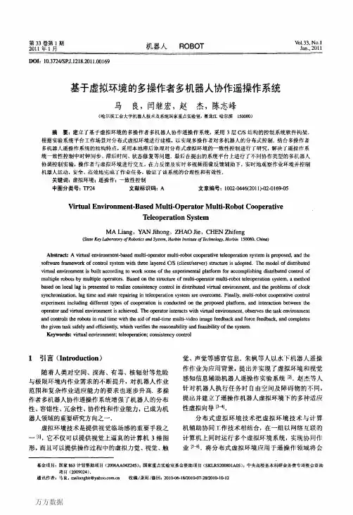
基于虚拟环境的多操作者多机器人协作遥操作系统作者：马良， 闫继宏， 赵杰， 陈志峰， MA Liang， YAN Jihong， ZHAO Jie， CHEN Zhifeng 作者单位：哈尔滨工业大学机器人技术及系统国家重点实验室,黑龙江,哈尔滨,150080刊名：机器人英文刊名：ROBOT年，卷(期)：2011,33(2)被引用次数：2次参考文献(9条)1.Burdea G C Invited review:The synergy between virtual reaIity and robotics[外文期刊] 1999(03)2.刘伟军;朱枫;董再励虚拟现实辅助机器人遥操作技术研究[期刊论文]-机器人 2001(05)3.闫继宏;赵楠;赵杰基于适应性虚拟向导的遥操作机器人系统[期刊论文]-哈尔滨工业大学学报 2007(01)4.赵杰;高胜;闻继宏基于虚拟向导的多操作者多机器人遥操作系统[期刊论文]-哈尔滨工业大学学报 2005(01)5.Cheng J P Research on distributed virtual environment based on web 20096.Ali A E E;El-Desoky A I;Salah M An allocation management algorithm for DVE system 20097.Chong N Y;Kotoku T;Ohba K A collaborative multi-siteteleoperation over an ISDN 2003(8/9)8.Chong N Y;Kotoku T;Ohba K Remote coordinated controis in multiple telerobot cooperation 20009.Alencastre-Miranda M;Munoz-Gomez L;Rudomin I Teleoperating robots in multiuser virtual envirorLments 2003本文读者也读过(3条)1.李珺.潘启树.周浦城.洪炳镕.LI Jun.PAN Qi-shu.Zhou Pu-cheng.HONG Bing-rong未知环境下多机器人协作追捕算法[期刊论文]-电子学报2011,39(3)2.刘利枚.蔡自兴.LIU Li-mei.CAI Zi-xing粒子群优化的多机器人协作定位方法[期刊论文]-中南大学学报（自然科学版）2011,42(3)3.丁滢颍.何衍.蒋静坪基于蚁群算法的多机器人协作策略[期刊论文]-机器人2003,25(5)引证文献(2条)1.王殿君移动机器人网络遥操作系统设计[期刊论文]-机床与液压 2013(9)2.李波.赵怀慈.孙士洁.花海洋空间机器人遥操作预测仿真系统研究[期刊论文]-计算机工程与设计 2013(10)引用本文格式：马良.闫继宏.赵杰.陈志峰.MA Liang.YAN Jihong.ZHAO Jie.CHEN Zhifeng基于虚拟环境的多操作者多机器人协作遥操作系统[期刊论文]-机器人 2011(2)。

DOI: 10.3785/j.issn.1008-973X.2021.05.004基于临场感的遥操作机器人共享控制研究综述陈英龙1,2，宋甫俊1，张军豪1,2，宋伟3，弓永军1,2(1. 大连海事大学 船舶与海洋工程学院，辽宁 大连 116026；2. 大连海事大学 辽宁省救助及打捞工程重点实验室，辽宁 大连 116026；3. 浙江大学 海洋电子与智能系统研究所，浙江 舟山 316021)摘 要：共享控制策略作为基于临场感的遥操作机器人的主要控制模式，能够充分利用操作者的感知、判断和决策能力，也能发挥出机器人自身的优势. 阐述遥操作机器人临场感技术；综述遥操作共享控制策略的发展现状，主要基于触觉反馈引导、运动学限制规避以及共享因子分配等，对各控制策略的原理进行介绍，并梳理和分析遥操作共享控制策略发展中的瓶颈和不足，如共享因素的单一化或僵硬化、时延问题和机器人自主判断能力有限等问题. 针对研究存在的局限性，从3个方面对未来的发展提出展望，分别为提升干预水平、加强机器人意图预测、结合机器学习, 具有一定的指导意义.关键词： 遥操作；共享控制；临场感技术；控制策略；共享因子；触觉反馈中图分类号： TH 11 文献标志码： A 文章编号： 1008−973X （2021）05−0831−12Telerobotic shared control strategy based on telepresence: a reviewCHEN Ying-long 1,2, SONG Fu-jun 1, ZHANG Jun-hao 1,2, SONG Wei 3, GONG Yong-jun 1,2(1. Naval Architecture and Ocean Engineering College , Dalian Maritime University , Dalian 116026, China ;2. Key Laboratory of Rescue and Salvage Engineering Liaoning Province , Dalian Maritime University , Dalian 116026, China ;3. Institute of Marine Electronics and Robotics , Zhejiang University , Zhoushan 316021, China )Abstract: The shared control strategy, as the main control mode of teleoperation robots based on telepresence, canmake full use of the operator's perception, judgment and decision-making ability, and utilize to the robot's own unique advantages. The telerobotic telepresence technology was introduced. The development of teleoperation shared control strategy was summarized. The principles of each control strategy were introduced mainly based on tactile feedback guidance, kinematic constraint avoidance and sharing factor assignment. The bottlenecks and shortcomings in the development of telerobotic shared control strategy were analyzed, such as the singleness or rigidity of shared factors, time delay and limited autonomous judgment ability of robots. The future research trends were proposed from three aspects in view of the limitations of the current study, namely, improving the intervention level, strengthening robot intention prediction, and combining machine learning, which have a certain guiding significance.Key words: teleoperation; shared control; telepresence technology; control strategy; shared factor; tactile feedback随着机器人技术的不断发展，在许多对人类不利的环境中执行任务时，依靠遥操作机器人既可以避免操作中的危险，又降低操作成本，提高了作业质量和效率[1]. 在过去的几十年里，关于机器人的智能自主性研究取得了不小进步. 然而，在目前可用的技术条件中，由于非结构环境的制约、人工智能和环境重构等相关限制，机器人自主化操作方式并不能保证任务安全、准确、平稳收稿日期：2020−11−02. 网址：/eng/article/2021/1008-973X/202105004.shtml基金项目：国家自然科学基金资助项目（51705452，51905067，U1908228）；工业和信息化部高科技船舶资助项目（2018ZX04001-021）；大连市科技创新基金重点学科重大资助项目（2020JJ25CY016）.作者简介：陈英龙（1984—），男，副教授，博士，从事流体传动及控制、机电系统高级运动控制和机器人技术研究./0000-0002-2149-093X. E-mail ：*********************.cn通信联系人：弓永军，男，教授，博士. /0000-0001-7665-7111. E-mail ：*******************第 55 卷第 5 期 2021 年 5 月浙 江 大 学 学 报(工学版)Journal of Zhejiang University (Engineering Science)Vol.55 No.5May 2021地完成，纯自主化机器人仍然具有挑战性[2]. 相反，人类在动态环境或意外情况下可以做出更加灵活和全面的反应. 对于如医疗手术、家庭服务、康复辅助等任务而言，既需要机器人的自动化，也要求训练有素的人员的专业知识，而完全自主系统一直以来受到安全、法律、成本等因素的限制[3-4].遥操作机器人技术允许人类扩展他们的物理能力，使人类能够实现干预操作或在对人类不利的环境中执行任务[5].自从1954年Goertz等[6]介绍了第1套机械驱动的遥操作机器人系统以来，遥操作机器人领域取得了较大进展. 在早期遥操作系统中，传感和控制由操作者本身掌握，操作者包含在底层的控制环中，远端机械臂在操作者的直接控制之下，不具有任何自主功能. 如在最早的遥控焊接实验中，通过夹持器夹持焊枪，再附带简单的距离保持器来完成核环境、水下环境、空间环境和其他极限环境下的遥控焊接[7]. 针对从端自主焊接控制不足的问题，哈工大通过对遥控焊接任务空间从宏观到微观的分析，建立焊接遥操作的人机协作智能分配模型，提出“宏观遥控、局部自主”的控制思想，设计遥控焊接任务的控制策略——人机协作控制策略[8]. 类似的遥操作机器人研究还有医疗手术辅助机器人[9]、水下机器人（remote op-erated vehicle，ROV）[10]、空间机器人[11]及灾难搜救机器人等[12]，它们的基本结构都是由人类操作员通过操纵杆或替代设备如鼠标和手势指令来遥控制机器人执行任务.虽然遥操作机器人领域已经取得了巨大进展，甚至其中一些已经商业化，得以应用于实际，但操作人员指挥从端机器人的方式并没有太大的改变. 一般来说，操作者在对从端机器人在远程环境中的行为进行视觉监控的同时，直接向从机器人发出特定的指令，称之为直接遥操作，它经常给操作者带来沉重的认知负担[13]. 除此之外，操作者与遥控机器人之间通信的时延和带宽限制一直是制约遥操作系统性能的主要因素；在使用传统的遥操作系统时，操作者的2种重要感知（视觉和力觉）被剥夺，严重影响操作者完成遥操作任务的能力[14]. 尤其是面对非结构环境、突发的事故时，人类操作者不能够及时处理问题，会降低任务成功率，甚至给用户带来人身安全隐患，也会使得操作者处于高度紧张状态，易产生精神疲劳，降低工作效率.为了解决上述问题，科研人员进行了许多研究，大致可以归为2类：其一，结合基于视觉、触觉、肌肉神经等感知信号的人机交互技术的特殊性能，能提高遥操作机器人系统的工作效率和控制精度[15-17]；其二，针对性地研究开发人机遥操作控制模式，充分发挥人类操作者与机器人各自的优势，在缓解人类操作者疲倦的同时提高系统的灵敏度、精确度，实现人机任务合理配置[18-19]. 目前，遥操作技术研究的相关综述侧重于人机交互技术的应用和人机交互下的共享控制系统发展，对于遥操作技术和控制策略的研究现状还未有详细的总结性报道[20].本研究概述遥操作机器人技术——临场感技术，分析其主要优势和应用特点；结合遥操作临场感技术对不同类型的遥操作机器人的共享控制策略进行总结，归纳出3个关键研究方面；着重对遥操作共享控制的未来发展进行探究，旨在为后续研究人员提供一定的参考.1 临场感技术在实际应用中普适性最高的技术是临场感技术（telepresence），主要可以分为2种：力反馈技术和虚拟现实技术. 两者的作用都是为了提高人类操作者遥操作过程的临场感能力. 作为新一代遥操作机器人系统的重要组成部分，临场感的核心理念在于为人类操作者提供身临现场的浸入式感官辅助，从而显著提高遥操作机器人完成复杂作业任务的效率[21].2006年Hokayem等[22]对临场感技术进行了相关综述. 宋爱国等[23-26]对相关领域进行了出色总结，自2013年起从4个方面对力觉临场感遥操作机器人进行了综述性分析. 综合考虑已有研究，临场感技术涵盖所有可以辅助提高人类操作者感知的方法，如触觉感知[27]、视觉感知[28]、脑机交互[29]等. 这些感知可以独立应用到机器人系统中，又可以通过互相配合提高系统多感知的能力，在环绕和避障任务的研究中很常见. 在遥操作应用中，以力反馈和虚拟现实为备受关注的研究热点.1.1 力反馈技术触觉感知的研究以临场感为代表. 触觉是许多遥操作机器人系统中不可缺少的一环，尤其在精度要求、控制安全要求高的场景. 力反馈技术832浙 江 大 学 学 报（工学版）第 55 卷是典型的临场感技术，其研究与应用更是与遥操作发展息息相关. 总而言之，现今的遥操作应用都包含力反馈内容，如图1所示为市场上较大众的力反馈设备.研究发现力反馈系统在克服时延影响方面发挥着重要的作用. 在面对低延迟时，利用波动变量和散射变换方法来解决[30-31]. 针对几秒或十多秒的通信延迟问题，Tanwani 等[32]提出模型预测的解决方法，根据设置的远程环境和机器人的几何和动力学模型，得到模拟视觉和实时的力反馈.在模型预测的基础上，Liang 等[33]提出人机协同半自主遥操作控制策略，不仅提高了操作精度，还可以减少操作人员的工作量. 结合模型预测和力反馈技术，王泓澈等[34]对大时延状态的带力反馈的主从式遥操作系统的控制器进行研究，通过单自由度力反馈遥操作系统的建模和分析，采用引入模型预测的方法对反馈力进行预测，减少时延对力反馈遥操作系统的操作性与稳定性的影响. 总的来说，利用力反馈预测可以在确保系统稳定的基础上削弱时延对系统性能的影响，并且有效提高遥操作系统的透明性和可操作性[35].因此，引入力反馈技术可以加强系统的抗干扰性. 张建军等[36]基于力反馈技术提出双边自适应阻抗控制，解决存在的机械手关节摩擦以及外部不确定干扰引起的模型不确定的问题. 甚至有的研究是将力反馈混合控制，达到提高主从异构型遥操作系统的稳定性和安全性的目的[37]. 相关的研究还包括如何减少主从两端干扰、误差影响方面研究.显而易见，力反馈技术并不限于提升机器人操作者的临场感知能力，在降低时延以及克服外在干扰方面也扮演着重要角色，还能优化系统安全性，更好地完成遥操作任务，减轻操作者工作负担.1.2 虚拟现实技术虚拟现实技术(virtual reality ，VR)是改善遥操作机器人工作效率的技术，作为提升临场感的关键技术，在遥操作的研究中占有较大比重. 虚拟现实技术是目前被认可的可以彻底解决网络时延问题最有效的方法，并在遥操作应用中得到证明[38].虚拟现实技术根据实际性能特点可以分为2种：虚拟环境技术和虚拟夹具技术. 前者是构建一个与从端类似的三维虚拟环境，从而避免主从通讯延迟引起的消极影响；后者在从端建立虚拟约束，既解决遥操作模式下的不足之处（如可视环境狭窄、延迟易导致反馈信息缺失），又能引导人类操作者实现避障、跟踪、路径优化等任务，提高工作效率和引导精度.虚拟环境能够在主端模拟一个与从端类似的三维虚拟环境，该环境容纳预设信息与从端反馈的传感器信息，使得全端与从端环境达到完全一致. 因此，在遥操作过程中，操作者可以直接通过人机交互设备与虚拟现实环境进行交互，能够实时产生视觉、听觉、触觉、力觉等感知，同时交互指令也可以被同步发送到从端，从而忽略时延干扰，达到真正的无时延交互的目的[39].虚拟夹具根据构型以及引导特性进行分类，虚拟夹具可以分为刚性、柔性虚拟夹具，前者在辅助机械臂的运动中具有引导速度快、引导精度高的优点；后者则更适应于处理空间复杂问题[40].刚性虚拟夹具构建方法主要有：基于点结构、基于线结构[41]、基于曲面结构[42]、基于几何体结构[43]和基于点云结构[44]等，它们的特点在于夹具的构型各不相同. Rosenberg [45]最早提出应用于遥操作手术、空间维护领域的虚拟夹具技术，在虚拟空间构建类似机械刚性夹具的约束，实现基础的人机共享操作，成功解决遥操作系统中的环境交互问题. 随着相关研究的不断深入，柔性虚拟约束也被广泛研究. 科研人员利用虚拟场分别构建作业对象及环境，构建对机器人的虚拟吸引力、虚拟排斥力，并通过力反馈设备实现虚拟夹具/约束[46].2 基于临场感的共享控制策略研究传统的遥操作技术本身具有一定的人机协作/协商/共享的特性，“共享”的概念既体现在遥操作控Omega SigmaLambda Delta图 1 常见力反馈设备Fig.1 Common force feedback devices第 5 期陈英龙, 等：基于临场感的遥操作机器人共享控制研究综述[J]. 浙江大学学报：工学版,2021, 55(5): 831–842.833制中，又体现在人机交互的过程中. 临场感加深了这个概念层次的表现，而基于此的共享控制策略更是被誉为带有鲜明的人机共享特色的控制模式. 这2种技术均为遥操作技术的重要组成部分，两者的融合能够提升遥操作机器人系统共享效果，是目前的研究热点和趋势.2.1 共享控制策略的发展遥操作机器人研发至今，其控制性能一直受时滞、环境反馈、人机交互方案低效等因素的影响.为了解决这些限制，国外很早就对共享控制展开研究，主要是作为研究设计较为直观的机器人遥操作系统的一种方法. 共享控制的概念最早是Sheridan[47]提出的，含义是指人、自主控制系统之间进行协调，共同对远端的机器人进行控制的控制策略. Sheridan[47]将共享控制方法引入机器人领域，机器人的不同自由度分别由手动和自动方式进行控制，人机各自完成任务，能够减轻操作员的负担，提高工作效率，并确保机器人控制的安全性、可靠性和稳定性. 该概念源于“遥操作”和“机器人”两者的有机结合，也就是说，机器人既能在遥操作下运行，也能在自主控制下运行[48].如图2所示，遥操作机器人控制方式主要为完全手动、半自主和全自主3种. 其中，完全手动控制因连续死板的低级操作而不被提倡，全自主控制由于安全隐患又不太现实. 因此，半自主控制成为当前遥操作机器人的主要控制方式和研究热点[49]. 不难看出，遥操作半自主控制与临场感之间的关系是互补的，通过虚拟现实技术和感知反馈技术，遥操作机器人系统实现了深度共享，在加深操作者浸入感的同时提高人机共享的程度.根据人机任务分配大小，常用的半自主控制主要有直接控制、监督控制和共享控制，如图3所示. 在直接控制中，从端完全跟随主端运动，所有决策都由操作者完成；在共享控制与监督控制中，它们的典型特征是2个控制环节：不包含操作者的远端控制环(内环)和包含操作者的整个系统控制环(外环). 图中，实线和虚线表示控制智能分配规模的程度，实线表示连通，虚线表示部分连通. 监督控制的特点是操作者不参与底层控制，只在上层监督；共享控制通过人机共享，实现高级决策（操作者）和底层动作（机器人）相结合的控制方式. 共享控制既具备直接控制和监督控制的优势，又避开了两者的不足之处[50]，表现如下. 1）根据系统的任务环境的即时信息，操作者可以如直接控制一般，利用自身感知、决策能力，通过人的智能实现高适应性，进而提高系统的安全性，避免自主控制误判失误操作引起的隐患. 2）也能和监督控制一样，将时延排除在底层控制回路之外，从而在局部获得较高的稳定性和控制精度.此外，在时延环节施加时延控制方法，能克服时延对遥操作系统稳定性和透明性的影响[51]. 3）引入协商操作机制，将机器人机械装置的精确控制能力与操作者的宏观决策能力集成起来，实现对机器人的高精度控制[52]. 尤其在高控制精度要求的遥操作场所，共享控制既可以利用机器人自主精细控制，又能发挥出操作者的引导判断能力.共享控制策略强调遥操作机器人系统的自主能力存在一定的局限性，故应当发挥操作人员智能水平，以达到操作者与机器人智能水平的平衡.具体操作是将协商操作机制引入该模型之中，即从端尽可能发挥其自主规划能力. 为了保证操作图 2 遥操作主要技术概述Fig.2 Overview of teleoperation techniques图 3 遥操作机器人控制模式Fig.3 Control mode of teleoperation robot834浙 江 大 学 学 报（工学版）第 55 卷执行的有效性，在从端执行具体动作之前，应向主端操作者提交即将执行的方案，且须经过主端操作者确认[53].共享控制也可以被理解为控制状态的角色切换，如“人主机辅”或者“人辅机主”，然而共享控制的协商机制是各不相同的. 王兴华等[54]提出基于行为的自主/遥控水下机器人（autonomous un-derwater vehicle ，AUV ）共享控制方法，通过设计的基于优先级的行为组织和融合方法，实现水下机器人以“人主机辅”模式执行环境探索，继而以“人辅机主”模式执行目标观察过程的有效共享.2.2 基于临场感的共享控制策略的研究方法在早期的共享控制策略中，人类操作员实际上只负责将高水平、直观的目标传递给机器人，由自主控制器将这些目标转换为运动指令，使得操作人员和自主控制器之间机器人系统的共享成为可能. 因此，如何实现人工操作者和自主控制器之间的角色划分，在很大程度上取决于任务本身、机器人系统和应用.C T C H C C C fe 如图4所示为传统的基于临场感的共享控制策略框架. 图中，、、分别为任务指令、人类指令和机器人指令；为反馈信息，既可以表示传感器反馈信息，也可以是人类操作者获取的信息.共享控制涉及了2个关键问题：1）什么时候应该混合使用这2个命令，使得遥操作指令与独立控制指令有效结合；2）如何修改每个命令. 因此，共享控制策略的核心内容可以分为两部分：1）选择/设计自主计划/控制方法（任务规划）；2）选择/设计控制方案（控制策略算法）.近年来遥操作的共享控制策略相关研究，与遥操作临场感技术——力反馈技术和虚拟现实技术紧密相关. 根据临场感技术和控制策略的实现原理，共享控制策略研究方法被分类归纳为以下3个方面：触觉反馈与引导（tactile feedback andguidance ，TFG ）、运动学规避限制（kinematic avoid-ance constraint ，KAC ）和共享因子分配（shared factor assignment ，SFC ），分析结果如表1所示.可以看出，大部分研究具有鲜明的针对性、专一性和应用性，往往都是对于某个类型遥操作机器人或者机器人系统设计或开发的一套共享控制策略算法. 然而，这三者之间其实是相辅相成的，事实上没有割裂独立，都与遥操作关键技术有联系，只是所侧重的研究方向不同. 体现出共享控制策略的研究范畴还是较大的，均涉及到上述的遥操作临场感技术.2.2.1 基于触觉反馈与引导　恰如骑马的这个比喻[74]，触觉共享控制能够给操作者提供更加直观的感知能力，使其能够更好地了解从端空间操作情况. 结合触觉反馈，当操作员远离任何物体时，只能收到关于存在不安全运动学构型的触觉反馈——关节极限和奇点；当目标在预先定义的距离内时，操作者则开始收到触觉提示，被引导做出最优姿态[75]. 换言之，触觉反馈可以近似为一个运动学约束，操作者则被提供类似动觉和振动的触觉反馈.甚至，若这些反馈引导操作者一个抓握的姿势，则只提供动觉反馈[76].总而言之，触觉共享控制的表现形式可以理解为在操作空间内给予从端机器人移动的指示信息（如禁区或禁行区），操作者根据机器人的指示信息改变移动指令. 如图5所示[77]为解决核环境下物体抓取的典型的触觉共享控制策略框图. 通过视觉反馈对点云（场景）进行抓握引导，同时操作者通过动觉反馈重新修正输入（重构）. 基于触觉的共享控制策略解决了多目标触觉引导问题，可以在不依赖概率估计或意图识别模型的情况下，确保平滑连续的目标抓取引导.除此之外，基于触觉的共享控制策略还能通过计算位姿极限或者奇异点的代价函数代替直接提供移动的提示指令，从而计算出最佳位姿以及施加在操作者手上的力信号. 基于此，Selvaggio 等[78]提出触觉引导的共享控制方法，解决在微创外科机器人执行缝合任务时，外科医生由于配置奇异点和关节限制而重新抓针的问题. 在整个触觉共享过程中被机器人告知最佳的抓取姿态/路线，操作者则最终控制机器人并做出决策选择何种抓取姿态/路线，从而考虑到其他非结构目标，避免不必要的操作，提高执行效率.除了上述触觉共享控制的研究外，Mario 等[79]图 4 基于临场感的共享控制框架Fig.4 Shared control framework based on presence第 5 期陈英龙, 等：基于临场感的遥操作机器人共享控制研究综述[J]. 浙江大学学报：工学版,2021, 55(5): 831–842.835将触觉引导与双边共享控制算法相结合，设计了基于触觉的人与机器人、机器人与环境的双边共享控制策略. 通过人机共享和双臂协调，在方向控制和避碰上进一步简化抓取任务的执行，使得人机的优势都能得以充分利用. 一些研究则通过融合人工力场（artificial force field，AFF)和虚拟阻抗力场（virtual impedance force field，VIF)，建立操作者、机器人及环境的交互界面. 相关研究[80]已经证明在遥操作过程中基于触觉的双边共享能够更好地应对复杂可变的操作空间，且可处理突发情况更广.综上考虑，从控制末端执行器的操作人员的角度来说，基于触觉的共享控制策略将远程机械手转向所需的目标位姿变为一项相当简单的任务. 主要体现为：1）既解决2个位置的复杂性问题，还调节了方向；2）解决若干约束条件（例如碰撞、关节极限、奇点）下对操作人员机动灵活性的限制（操作人员可以有直接或直观的意识）；3）不仅适应于静态的工作环境，也适用于动态的有障碍的环境.2.2.2 基于运动学限制规避　最近，在协作机器人研究中，运动学限制规避已经被成熟地用来改善性能和进行直观的物理人机交互. 在机器人遥操作中，这种方法也是通用的. 须解决的问题是：在不提供高保真的触觉反馈条件下，能够反映从端与环境之间的实际物理接触，而且为人类操作者表 1 共享控制策略研究简要汇总Tab.1 Brief summary of research on shared control strategy文献应用场景TFG KAC SFA研究特点[55]轨迹规划*权重由操作者当前输入动作和目标物体的距离决定[56]椎弓根螺钉固定手术**外科医生可以直接控制攻丝轴上的相互作用力/扭矩，而不会降低其他方向上的位置精度[57]远程操作热线工作**操作者和自主运动规划器共同生成笛卡尔任务轨迹[58]复杂环境避障、导航**考虑机器人与障碍物之间的距离，从而分别确定柔性控制器和导航控制器合适的合作权值[59]核电站高位重水更换*操作员仅控制从属机器人，而抑振任务分配给机器人系统[60]微创手术(MIS)*外科医生全程控制工具的位置，并得到系统的支持，即外科医生感觉到力，但同时不阻碍或影响手术过程[61]六足机器人爬梯**操作者和自主控制器的命令交由共享控制器中的控制权重函数进行处理[62]机器人避障**以稳定裕度与稳定裕度变化率为输入，共享因子为输出的模糊控制器，实现变权重共享控制[63]空间远程操作**根据操作员和自主控制模块的作用大小取加权融合[64]双臂协同**2名操作者通过优势因子调节各操作者的控制权重[65]无人机飞行任务**融合人主动操作和机器人自主运动的共享控制策略，使得机器人的控制权限可以在人和机器人之间平滑转移[66]辅助避障**人的权重和机器人的权重是分别受不同因素影响的[67]动态工作空间搬运*分别研究共享控制中提高机器人自主运动能力和辅助操作者提高操作能力的方法[68]ATRV机器人**遥操作系统允许人类扩展他们的物理能力，使他们能够干预危险操作或在他们不可能存在的地方[69]QBot机器人移动**同时考虑机器人的自主性和人的干预，通过阻抗和导纳模型保证从人的操作到机器人运动的无源性[70]手术教学引导**外科医生之间共享的控制权限是根据他们相对水平的手术技能和经验来选择的[71]非结构环境的探索***不仅根据给定环境上下文，而且根据用户当前行为的上下文来调节共享控制器提供的辅助水平[72]自由飞行太空机器人（FFSR）**将地面操作员的决策能力与空间机器人的自主能力有效地结合起来实现对目标更有效的捕获[73]微创外科手术(RMIS)**人工势场结合虚拟代理点，限制机器人执行机构的运动836浙 江 大 学 学 报（工学版）第 55 卷。

合肥研究院高层次人才招聘推荐（自荐）表
招聘单位合肥研究院智能机械研究所申报类别创新岗位研究员
申报学科(二级学科) 控制科学与工程
姓名高理富
工作部门仿生感知与控制研究中心
中国科学院合肥物质科学研究院
二○一○年七月
说明
一、请申请者实事求是地填写表中内容。

二、申请者除填写此表外，还需附发表文章的收录和引用情况的检
索证明、1－3篇代表性论文复印件、国外任职情况证明材料、博士学位证书及本人认为有必要提供的相关材料。

三、申请人联系地址及电话：
地址EMBL Hamburg c/o DESY, Notkestr 85, 22603 Hamburg, Germany
电话+49 40 89902- 241
传真+49 40 89902 106
E-mail lifuao@embl-hamburg.de
论文被收录情况统计
论文被引用情况统计
注：1. 论文被收录与引用的统计年度范围以申请年度前5年为限；
2. 自引部分不计入引文统计中;
3. 对列入统计表中的论文及引文均需附清单（作者、刊物
名称、年、卷（期）、起止页码）；
4. 请出据论文被引证明。

Teleoperation of ABB Industrial RobotsMohsen Moradi Dalvand and Saeid NahavandCentre for Intelligent Systems Research (CISR), Deakin University, Waurn Ponds Campus, AustraliaAbstractPurpose – This paper analyses teleoperation of an ABB industrial robot with an ABB IRC5 controller. A method to improve motion smoothness and decrease latency using the existing ABB IRC5 robot controller without access to any low level interface is proposed.Design/methodology/approach –The proposed control algorithm includes a high-level PID controller used to dynamically generate reference velocities for different travel ranges of the tool centre point (TCP) of the robot. Communication with the ABB IRC5 controller was performed utilising the ABB PC software development kit (SDK). The multitasking feature of the IRC5 controller was used in order to enhance the communication frequency between the controller and the remote application. Trajectory tracking experiments of a pre-defined 3D trajectory were carried out and the benefits of the proposed algorithm was demonstrated. The robot was intentionally installed on a wobbly table and its vibrations were recorded using a six degrees of freedom (DOF) force/torque sensor fitted to the tool mounting interface of the robot. The robot vibrations were used as a measure of the smoothness of the tracking movements.Findings – A communication rate of up to 250 Hz between computer and controller was established using C# .Net. Experimental results demonstrating the robot tool centre point (TCP), tracking errors, and robot vibrations for different control approaches were provided and analysed. It was demonstrated that the proposed approach results in the smoothest motion with less than 0.2 mm tracking errors.Research limitations/implications – The proposed approach may be employed to produce smooth motion for a remotely operated ABB industrial robot with the existing ABB IRC5 controller. However, in order to achieve high-bandwidth path following, the inherent latency of the controller must be overcome, for example by utilising a low level interface. It is particularly useful for applications including a large number of short manipulation segments, which is typical in teleoperation applications.Social implications – Using the proposed technique, off-the-shelf industrial robots can be used for research and industrial applications where remote control is required.Originality/value – Although low-level control interface for industrial robots seem to be the ideal long-term solution for teleoperation applications, the proposed remote control technique allows out-of-the-box ABB industrial robots with IRC5 controllers to achieve high efficiency and manipulation smoothness without requirements of any low-level programming interface.Keywords - Robotics, Teleoperation, Remote control,PID controller, Trajectory tracking, Force/torque sensor, VibrationIntroductionIndustrial robot manipulators are relatively cheap and mechanically optimised (Hirzinger et al., 2005, Brogårdh, 2007) and are therefore frequently utilised for both industrial applications and research projects (Desbats et al., 2006, You et al., 2012, Moradi Dalvand and Shirinzadeh, 2013). Commercial industrial robotic systems typically provide a static off-line programming interface (Xiao et al., 2012). Although off-line programming is sufficient for most industrial applications, some applications including teleoperation and force-guided manipulation require a more flexible and dynamic approach to incorporate online trajectory generation and path planning into the control architecture (Xiao et al., 2012, Cederberg et al., 2002, Nilsson and Johansson, 1999). In on-line control applications, new information including set points of the trajectory are calculated on-line from a remote client and sent to the controller “on-the-fly” (Neto et al., 2010). This approach enables the control architecture to react instantaneously to unforeseen events. Teleoperation applications typically involve a large number of short displacement commands executed consecutively. For force-controlled manipulation and teleoperation applications in stiff environments, control rates of more than 1 kHz are essential to avoid damaging the robot and its environment and to improve control stability/quality or perceptual stability, respectively (Cederberg et al., 2002, Kubus et al., 2009, Kroger et al., 2004, Moradi Dalvand et al., 2013, In press). Especially for high approach velocities and stiff environments, high update rates and low delays are key requirements for stability and thus for realistic haptic perception (Kubus et al., 2009). Different control techniques have been studied and investigated for teleportation of robot manipulators requiring direct access to motor controllers including feed-forward control, trajectory pre-filtering, and predictive control (Slama et al., 2007, Slama et al., 2008, Torfs et al., 1998). In the literature, to the best knowledge of the authors of this article, very limited research has been conducted to study and analyse control techniques to improve the smoothness and decrease the latency of the movements of off-the-shelf industrial robots for teleoperation applications (Cederberg et al., 2002, Li et al., 2003).While commercially available manipulators generally offer favourable mechanical and electrical characteristics for control-related research, the provided control interfaces do not allow for high-rate low-level control (Blomdell et al., 2005). The robot controllers provided by manufacturers typically lack high-rate low-latency communication interfaces and only provide control intervals in the two-digit millisecond range (Kubus et al., 2010). In ABB robot controllers, the delay between when a movement instruction executes and the time at which the robot moves comprises of the time it takes for the robot to plan for the next movement (approximately 0.1 s) and the servo lags (0-1.0 s depending on the velocity and the actual deceleration performance of the robot) (ABB-Robotics, 2000). Often the performance of robotic systems and the quality of research results can be improved significantly by employing an appropriate low-level control interface instead of the original controller (Kubus et al., 2010). Therefore, the main focus of the researchers in this field in the last decade have been concentrated on the development and implementation of low-level interfaces to the robot hardware in order to overcome the limitations of the commercially available control systems for the industrial robot manipulators (Kubus et al., 2010).Several suppliers of industrial robots have introduced a possibility of interoperability of their robot controllers with control algorithms executing on external computers and developed new control interfaces enabling open communication channels with rates higher than 1 kHz. Such communication channels allow the users low-level access (with given limits) to the control strategies of the commercial devices. Mitsubishi developed an optical ARCNet communication channel to the PA-10 robot arm with 400 Hz communication rate (Artemiadis and Kyriakopoulos, 2006). COMAU Robotics introduced a new policy and changed the open version of the industrial COMAU C3G 9000 controller produced by Tecnospazio into a partially opened C3G control system (Lippiello et al., 2007). KUKA Roboter GmbH introduced a real-time Ethernet channel at 1 kHz for the third generation of DLR lightweight robots (LWR III) (Albu-Schäffer et al., 2007). Finally, Staubli introduced a Low Level Interface (LLI) that allows an easy interface to the low level control loop and is integrated with CS8C controllers (Pertin and Bonnet des Tuves, 2004).Modifying commercial robot controllers or developing open robot controllers for commercial manipulators requires advanced knowledge in several fields and is difficult to achieve without compromising safety. Although low-level control interfaces seem to be the ideal long-term solution for applications like teleoperation, very little has been published about short-term solutions or methods to improve the performance of the current built-in commercial control systems. Only limited information can be obtained from the manufacturers and robot suppliers, and very little research has been conducted to analyse thefunctional properties of industrial robots and controllers (Cederberg et al., 2002, Li et al., 2003). In one limited study directly dealing with remote control of the industrial robots, the response frequency of an ABB industrial robot with an S4C+ controller was found to be 10 Hz. (Cederberg et al., 2002). This study also proposed a control technique; however, no experimental results and validation were provided. In another research effort, remote control of an ABB industrial robot for meat processing applications was studied (Li et al., 2003). This study utilised an ABB IRB 4400 robot with an S4C+ robot controller to evaluate the accuracy and latency of multi-point non-continuous trajectory tracking for a remote application. Experimental results indicated two cases of 800 ms delay with low tracking errors and 150 ms latency in remote control responses with 10 mm tracking errors. The conclusion was that although commercial industrial robots can achieve good accuracy, the motion response of industrial robots does not support real time control and it is therefore impossible to adapt an industrial robot directly to an application with real time or quick response operation requirements.Figure 1 – Experimental setup including an ABB IRB 120 robot incorporated with a force/torque sensor, an ABB IRC5 robot controller, and a standard computer connected to the controller through Ethernet network Both of these studies have revealed that it is challenging to produce remote control motions with high accuracy and low delay; however, more research is required to investigate other control techniques for modern robot controllers like the ABB IRC5 controller with built-in PC-Interface and Multitasking features. This paper focuses on evaluation and improvement of control techniques for teleoperation of an ABB IRB 120 robot with the ABB IRC5 controller (Figure 1). The objective was to follow 3D trajectories continuously generated from a remote location. Extensive experiments using various control techniques were conducted and the results were analysed. The remainder of this paper is organised as follows: A brief explanation of the remote control techniques of industrial robots is introduced in Section 2 while Section 3 describes the experimental setup. In Section 4, experimental results are reported and analysed. Finally, conclusions are presented in Section 5.Control TechniqueABB PC software development kit (SDK) makes it possible for system integrators, third parties or end-users to add their own customised operator interfaces to the IRC5 controller. This allows flexible solutions and customised interfaces fitting the specific requirements of an operator (ABB-Robotics, 2000). Such stand-alone applications with customised interfaces are able to communicate with the real robot controller over a network or with a virtual robot controller in ABB RobotStudio. There are several restrictions for remoteclients and specific privileges must be acquired by requesting so-called “mastership” of the controller domain explicitly by the remote application. The IRC5 controller must also be in automatic operating mode. The remote applications are able to monitor and access one or several robot controllers from one location and are less limited in terms of memory resources and process power compared with “local” clients on the FlexPendant (ABB-Robotics).ABB PC SDK provides a set of services to monitor and control the robot. These services include connection, communication, file and task management services (Cederberg et al., 2002). The connection management services basically provide support for other services, for example start, stop, and restart of a connection. The communication management service is responsible for retrieving information from the robot controller and updating data of the robot controller, for example reading or modifying predefined persistent controller variables. The functionality to access files on the robot controller, for example to open, read, write, close, rename and delete a file is provided by the file management services. Finally, the task management service provides methods such as start, stop, and restart of RAPID tasks in single task or multitask configurations.Normally, a RAPID program is prepared for a particular application and all of its parameters are predefined, updated and used within the program execution loop. It is realised as a stand-alone program and typically has no communication with the outside world except for digital and analogue input and output. However, for some applications (e.g. teleoperation) the local RAPID program must communicate with a remote program in order to send and receive RAPID data. Figure 2 presents an overview of the control architecture used in this research. The external computer interacts with an executing RAPID program by updating RAPID data defined as persistent variables in the program. This interaction is achieved by a remote master-slave application developed by the ABB PC SDK. The RAPID program on the slave side typically includes a sequence of MoveL instructions whose parameters are modified by a remote master application. The MoveL instruction refers to a linear movement to a given destination (ABB-Robotics, 2000). Its arguments include v and z that denote TCP velocity and zonedata structures, respectively. Zonedata is used to specify how a position is to be terminated and how close to the programmed position the robot must be before moving towards the next ordered position.Figure 2 – Remote Control Architecture (RAB: Robot Application Builder, PERS: persistent)The pseudo code for the RAPID program and remote program proposed in this paper are listed in Table 1. In the RAPIDprogram, two variables, p1 and p2, of RobTarget structures are predefined and act as buffers for the variables being updated by the remote application. A RobTarget structure defines the position and orientation of the robot and external axes. As a robot is often able to achieve the same position and orientation of the tool with two or more axis configurations, the RobTarget structure also includes data tounambiguously define the axis configuration of the robot. In order to enable read and write of variables between multiple RAPID programs in multitasking programming, the variables are declared as persistent. During execution, the values of p1 and p2 are dynamically updated in a circular fashion with the data sent by the remote application. The remote application and the RAPID code are synchronised so that the remote application keeps track of which MoveL instruction is currently running and which RobTarget structure needs to be updated for the next MoveL instruction.In order to achieve smooth transition between consecutive linear movements between positions that are updated on-the-fly, the zone value should be used. If the argument fine is used instead of a zone value, the following move instruction is executed after the robot is standing still in its destination. This results in a jaggy motion. If instead a zone value is defined, the next MoveL instruction is executed before the robot has reached the target position. This produces the smooth transitional motions which are desired in teleoperation applications. Utilising the zone argument requires that the RobTarget structure for the next MoveL instruction is defined before the interpolator is finished with the first destination. For example, when the robot starts moving to p2, the next point (p1) must be defined.Table 1 – Pseudo code for the RAPID program and remote programRAPID Program Remote Program! VARIABLE DECLARATIONS proc IntelliMove(start,end) Dist:=Distance(start,end); vVar:=PID(Dist);MoveL end, vVar, z, tool0; Dist_pre:=Dist;ENDPROCproc Main()!INITIALISATION...WHILE NOT ABORTED DOWaitUntil Flag1=FALSE;IntelliMove pre_p2,p1;pre_p1:=p1;curP:=2;Flag1:=FALSE;WaitUntil Flag2=FALSEIntelliMove pre_p1,p2;pre_p2:=p2;curP:=1;Flag2:=FALSE;ENDWHILEENDPROC // VARIABLE DECLARATIONS ... getControllerMASTERSHIP(); startRAPIDTasks();while (true){getRAPIDData();if NOT IsChanged(curP) continue;switch (curP){case 2:updateRAPIDData(p1);updateRAPIDData(Flag2); case 1:updateRAPIDData(p2);updateRAPIDData(Flag1); }}On the other hand, initiating a MoveL instruction ahead of a robot movement may lead to executing multiple MoveL instructions with identical RobTarget structures. This leads to a stop which also causes jaggy motions. To avoid this problem, a mechanism was established in order to make sure that the RobTarget value of the next MoveL instruction has already been updated with a Robtarget different than the previous one before initiating a MoveL instruction. Variables Flag1, Flag2 and curP are defined in the remote application (Table 1) to make sure the update sequence of the RAPID data are one step ahead of the move instruction sequence. Once the next Robtarget and consequently the corresponding variable (Flag1 or Flag2) are validated from the remote application on the master side, the RAPID program that is continuously monitoring the variables Flag1 and Flag2 is notified. The variableFlag1 or Flag2 confirms that the next RobTarget has been updated and the next MoveL instruction can be initiated. The variable curP is set at this exact time to avoid re-validation of the variable Flag1 or Flag2 by the remote application.The positions of the RobTarget variables updated by the remote application are not equidistant. Resultsfrom the experiments performed in this paper show that the size of the programmed velocity has a profound effect on the motion quality. If the programmed velocity deviates too much from an optimal value, the resulting motion becomes very jaggy. In order to resolve this problem, a PID control algorithm was implemented to dynamically calculate the necessary velocity of the TCP according to the required travel distance. The procedure IntelliMove in the pseudo code for the RAPID program (Table 1) calculates the dynamically updating velocity according to the distance to the new target and initiates the MoveL instruction.Experimental SetupIn order to verify the validity and effectiveness of the proposed teleoperation control technique, trajectory tracking experiments for a time-varying 3D figure-eight curve shaped like an ∞symbol (also known as lemniscate of Gerono) were carried out. Figure 3 presents consecutive photos of the ABB IRB 120 robot during the trajectory tracking experiment. Highlighted photos represent the robot states at start, middle and end of the tracking trajectory. Furthermore, to compare the smoothness of the robot motion for different control parameters, the robot was installed on a wobbly table and the vibrations caused by the robot movements were used as a measure of motion smoothness. The vibrations were captured by a 6-DOF force/torque sensor from Sunrise Instruments (/) mounted at the tool mounting interface of the robot.As shown in Figure 1, the experimental setup includes an ABB IRB 120 industrial robot incorporated with a force/torque sensor, an ABB IRC5 robot controller, and a standard computer that is connected to the robot controller through Ethernet network. Software including Visual Studio .Net, ABB PC SDK components of Robot Application Builder (RAP) and ABB RobotWare were installed on the computer. The IRC5 robot controller was integrated with the option PC Interface, which is required for communication with an external computer. Trajectory tracking manipulations were performed by updating the RobTarget data structures one by one and submitting them to the RAPID program to process and initiate the MoveL instructions accordingly.Figure 3 – Consecutive photos of the robot during the trajectory tracking motionstarting from left to right and top to bottomExperimental Results and DiscussionTo evaluate the proposed control technique various tracking experiments with different velocities of the MoveL instructions were conducted. Experiments were performed both with constant speed and by dynamically updating the speed using the proposed PID controller. The constant velocities were chosen as 40, 50, 60, 80, 100, 200, 500, 1000 and vmax mm/s, where vmax is the maximum achievable TCP speed in the present configuration. As listed in Table 1, vVar is the dynamic velocity calculated using the PID controller. The calculation of vVar is based on the distances between the ordered spatial positions along the tracking path and the orientations of the TCP at those points are not involved. If the manipulation involves sudden changes in the orientations of the TCP, the calculation method should be modified accordingly.Figure 4 shows the experimental results for the robot TCP displacements for the constant velocities vmax, 500, 200, 100, 80, 60, and 40 mm/s. Figure 5 illustrates the desired and real trajectories of the TCP for these experiments in 3D. Tracking errors for these experiments are listed in Figure 6. The vibration of the robot measured by the force/torque sensor is used as a measure of the smoothness of the tracking motion. The robot vibrations in the form of the force measured by the sensor for all of the constant velocities are presented in Figure 7. The latencies of the robot movement with respect to the desired time-varying trajectory for different constant velocities with zone value and fine argument as well as the dynamically updating velocity calculated using the proposed PID controller are listed in Table 2.As shown in Figures 4a-4c (and 5a-5-c), the results for the velocities vmax, 500, and 200 mm/s are similar and all relatively jagged. For these high speed experiments, the robot TCP reached the destinations along the tracking path fairly quickly before executing the next MoveL instruction available to the controller. In other words, the update rate of the RobTarget data structures were slower than the robot movements. Hence, the robot had stationary states in different intervals waiting for the next commands to be ready, explaining the jaggedness in the movements. The reason of having similar results for these high speed experiments is that the control system reduces the programmed speed to what is physically possible. The duration of each experiment was around 17.5 s and the each tracking error was less than 0.2 mm (Figures 6a-6c). As shown in Figures 7a-7c, the vibration of the robot in each experiment was extreme with a maximum of around 9 N.The robot tracking movement was greatly improved with much smoother tracking motions by decreasing the velocity to 100 mm/s (Figures 4d and 5d). The results are still jagged in some parts of the tracking trajectory, depending on the travel distances for different RobTarget structures along the tracking path and so the robot vibration remained at a high level with a maximum around 9 N (Figure 7d). Also in these cases, the duration of each tracking motion was around 17.5 s and the tracking error less than 0.2 mm (Figure 6d).Table 2 – Robot movement latencies for constant velocities with zone value and fine argument as well as the dynamically updating velocity calculated using the proposed PID controller Speed Type Constant DynamicZone zone value fine zone valueSpeed (mm/s) vmaxto200100 80 6050to40vmaxto200100 80 6050to40vVarLatency (ms) 430380 542 2786 N/A 327 710 1553 3417 N/A 344When the speed was decreased to 80 mm/s, uneven and irregular delays appeared at different stages of the tracking experiment (Figures 4e and 5e) and no improvement was made in terms of vibration which remained at the maximum level measured by the sensor (around 9 N in Figure 7e). The total time of the experiment was also slightly increased to around 18 s (Figures 4e and 5e). The tracking errors due to the irregular delays had a large jump to around 1.7 mm at the maximum level (Figure 6e). These problems increased when the speed was decreased to 60 and 40 mm/s (Figures 4f, 4g, 5f, and 5g), respectively, with huge delays between consecutive MoveL instructions and much longer time for the entire robot movement (20.5 and 23 s, respectively). The corresponding tracking errors at the maximum level increased to around 32 and 40 mm (Figures 6f and 6g), respectively. However, the vibration of the robot for these low speed manipulations were decreased, resulting in smoother plots with maximum value reduced to around 5 and 3.5 (N) (Figures 7f and 7g), respectively. The minimum latency in the robot motion was measured around 380 ms for the constant velocity of 100 mm/s (Table 2 and Figures 4d and 5d).Figure 4 – TCP displacements for seven differentconstant velocitiesFigure 5 – Desired and real trajectories in 3Dforce/torque sensor mounted at the TCP of therobot for seven different constant velocitiesdifferent constant velocitieswith fine argumentsrobot vibration, and dynamic velocity calculatedusing the proposed PID controller Figure 8 presents the results for TCP displacements, tracking errors, and robot vibrations using the constant speed vmax and the argument fine in the MoveL instructions. As shown in this figure, this leads to a very jagged tracking movement (Figure 8a) with the largest vibration of all the simulations (Figure 8c). However, this case also has the lowest tracking errors of all simulations (Figure 8b). The reason why the tracking errors are minimised in this case is that when a MoveL instruction is initiated with the argument fine, the robot does not process next instructions until the robot reaches the target. Therefore, no interpolation between the consecutive targets are used which minimises the tracking errors (Figure 8b). The manipulation latency using the constant speed vmax and the argument fine in the MoveL instructions was measured around 327 ms (Table 2 and Figure 8a).Figure 9 shows the experimental results for the TCP displacements, tracking errors, robot vibrations as well as the dynamics velocity calculated by the proposed controller PID using the proposed PID controller. The speed vVar was calculated on-the-fly and dynamically updated. As this figure indicates, this leads to a significantly smoother tracking motion compared with the best observed results for the constant speeds at 100 mm/s (Figure 4d and 5d). The tracking errors were less than 0.2 mm which are similar to the errors for the tracking motions with the constant velocities of 100 mm/s (Figure 6d) and higher (Figures 6a-6c). The amount of the vibration was also similar to the range of the vibrations for the low speed tracking motions with the constant velocities of 60 and 40 mm/s (Figures 7f and 7g). Figure 9 also illustrates the velocities calculated using the PID controller during the trajectory tracking experiment (Figure 7g). The manipulation latency using the dynamically updating velocity was around 344 ms (Table 2 and Figure 9).The experimental results imply that for each MoveL instruction, there exists one optimal constant TCPspeed which leads to the smoothest tracking motion. This specific speed depends on the type and time variance of the trajectory and employing a constant speed for all movements will therefore not be ideal neither in terms of smoothness nor in terms of vibration. Using a speed that is lower or higher than the optimal speed causes the stop-start scenarios, irregular delays and consequently jaggy or inaccurate motions shown in Figures 4-7. This issue was solved in the proposed control technique using the PID control algorithm designed to dynamically calculate the velocity according to the distance between the points along the desired trajectory (Figure 9). Using the proposed PID controller, the latency in the robot movements was also decreased from 420 ms for the constant velocity of 100 mm/s (Figures 4d and 5d) to 340 mm/s for the dynamically updating velocity.ConclusionDue to the inherent design of commercial robot control systems, industrial robots typically have limited capabilities for real time operations. Industrial robots typically exhibit a long delay between the time a motion is ordered and the robot actually moves. This latency makes standard industrial robots unsuitable for many applications requiring an immediate response to sensor inputs. However, this paper demonstrates that smooth motion with minimum latency can be achieved using a control technique based on circularly validating two pre-defined variables in the RAPID program using a remote application. Extensive experiments were conducted showing successful tracking motions with tracking errors less than 0.2 mm with constant speeds; however, the achieved motions were jaggy and caused lots of vibrations. To improve the motion smoothness, a PID control algorithm was introduced to dynamically update the programmed speed for the next consecutive motion based on the distance between ordered positions along the trajectory. It was demonstrated that this approach maintains good positioning accuracy and leads to a smooth tracking motion with minimised vibration and a latency of 344 ms. This result was achieved using the existing IRC5 robot controller without access to the low-level programs of the controller. The proposed control technique may be employed to remotely control industrial robots for applications in dangerous environments like nuclear power plants and microbial diseases laboratories, or any other application with hard and/or dangerous working condition.ReferencesABB-ROBOTICS PC SDK Application manual. ABB Robotics.ABB-ROBOTICS 2000. PC Rapid Reference Manual - Rapid Overview On-Line. ABB Robotics,3HAC 0966-50.ALBU-SCHÄFFER, A., OTT, C. & HIRZINGER, G. 2007. A unified passivity-based control framework for position, torque and impedance control of flexible joint robots. The International Journal of Robotics Research, 26, 23-39.ARTEMIADIS, P. K. & KYRIAKOPOULOS, K. J. Teleoperation of a robot arm in 2d catching movements using emg signals and a bio-inspired motion law. Biomedical Robotics and Biomechatronics, 2006.BioRob 2006. The First IEEE/RAS-EMBS International Conference on, 2006. IEEE, 41-46. BLOMDELL, A., BOLMSJO, G., BROGARDH, T., CEDERBERG, P., ISAKSSON, M., JOHANSSON, R., HAAGE, M., NILSSON, K., OLSSON, M. & OLSSON, T. 2005. Extending an industrial robot controller: implementation and applications of a fast open sensor interface. Robotics & Automation Magazine, IEEE, 12, 85-94.BROGÅRDH, T. 2007. Present and future robot control development—an industrial perspective. Annual Reviews in Control, 31, 69-79.CEDERBERG, P., OLSSON, M. & BOLMSJÖ, G. Remote control of a standard ABB robot system in real time using the Robot Application Protocol (RAP). Proceedings of the 33rd ISR (International Symposium on Robotics) October, 2002. 11.DESBATS, P., GEFFARD, F., PIOLAIN, G. & COUDRAY, A. 2006. Force-feedback teleoperation of an industrial robot in a nuclear spent fuel reprocessing plant. Industrial Robot: An International Journal, 33, 178-186.。

本文件界定了智能无人集群系统的架构、感知、控制、通信、任务和评估的术语和定义。

本文件适用于智能无人集群系统的设计、研制、使用和维护以及相关技术的贸易及交流。

本文件没有规范性引用文件。

在无人操作且有人监控情况下完成特定任务的系统。

示例：无人系统可以是移动的或固定的，包括无人地面设备、无人空中设备、无人水下设备、无人水面设备和其他使用智能传感器技术无人操作的设备及相关系统。

agent智能体代表另一个实体行动的实体。

unmanned swarm [system]一组共同自主、协调、鲁棒地完成特定任务的无人系统(3.1.1)。

异构[无人]集群[系统] heterogeneous unmanned swarm [system]具有不同属性的无人系统(3.1.1)组成的无人集群[系统](3.1.3)。

3.1.3.2同构[无人]集群[系统] homogeneous unmanned swarm [system]具有相同属性的无人系统(3.1.1)组成的无人集群[系统](3.1.3)。

3.1.4协调coordination通过无人系统(3.1.1)之间相互商定或由上级进行授权，指导或促进多个无人系统(3.1.1)的活1T/CESA 1192—2022动以完成某一任务的方式。

3.1.5协同cooperation合作多无人系统(3.1.1)基于信息、资源以及责任的共享机制合力规划、实施和评估，共同完成某一任务的方式。

3.1.6协作 collaboration无人集群[系统](3.1.3)中无人系统(3.1.1)配合其他无人系统(3.1.1)完成某一任务的方式。

3.1.7跨域协同cross-domain cooperation在陆、海、空、天及网络和电磁环境中联合执行任务，以协同方式共同完成任务。

3.1.8同构协同 homogeneous cooperation同构[无人]集群[系统](3.1.3.2)以协同方式完成任务。

第三届数字制造与自动化国际会议征稿通知2012年7月31日-8月2日（桂林）SCI、EI（1:2）第三届数字制造与自动化国际会议（ICDMA）(第一届，第二届数字制造与自动化会议均已被EI核心检索，第三届ICDMA将由应用力学与材料期刊(AMM)以及IEEE-CPS出版，并将被EI核心及ISTP检索)由上海师范大学，广西航空航天学会，中南大学，清华大学，国际机械促进联盟共同举办，将于2012年7月31日-8月2日在桂林召开，将邀请7-8名国际知名学者的国内外学者做关键发言，并与广西航空航天学会的年会一起召开，将有数十家相关企业参与，第二轮征稿录用论文将由IEEE-CPS出版，并将被EI和ISTP检索，并有总比例为2:1的比例推荐到SCI期刊（共约200篇）和高档次的Ei期刊，欢迎机械、电子、检测与传感、计算机、材料、控制类作者投稿，并欢迎各重点实验室主任、学院领导、教授进行组稿或者担任审稿专家。

重要日期：第二轮征稿截止日期;：2012年5月5号录用/拒稿通知：投稿后15天推荐的期刊列表：一、Ei 期刊：1）Sensors & Transducers journal (ISSN: 1726-5479) 传感器与变换2）Journal of Bionanoscience （ISSN: 1557-7910）生物纳诺科学二、SCI 期刊：1)Sensor Letters（ISSN 1546-198X，SCI+EI双源刊)；2)ADVANCED SCIENCE LETTERS (ISSN 1936-6612，SCI源刊))；3)Mechanika (ISSN 1392-1207 SCI+EI双源刊)；以上Ei期刊将会各出版我们约40篇论文,SCI期刊将出版约200篇论文(分期出)会议网址：论文格式：/some-related-imformation联系方式：Email: icmedm@Tel: +86-731 82618984+86-152********QQ群：222316287ICDMA'2012 SecretariatContributions covering theoretical developments and practical applications,including but not limited to the following technical areas are invited:A.Digital Manufacturing and Advanced Manufacturing1)Industrial automation, process control, manufacturing process and automation工业自动化，过程控制，制造过程自动化2)Advanced Manufacturing Technology, Sustainable Production, Recycling andRemanufacturing, Rapid Manufacturing 先进制造技术，可持续制造，循环和再制造，快速制造3)Micro-Machining Technology and Laser Processing Technology微细加工和激光加工技术4)Bionic Mechanisms and Bio-manufacturing仿生机械和生物制造5)Virtual Manufacturing and Network Manufacturing虚拟制造与网络制造6)High-speed Automation and Intelligent Control, Intelligent Manufacturing,Knowledge-based Engineering高速自动化与智能控制，智能制造与知识工程7)High-precision Manufacturing Automation Technology 高精度制造与自动化技术8)CAD/CAE/CAPP/CAM计算机辅助设计、计算机辅助工程、计算机辅助工艺过程设计、计算机辅助制造9)PLM, PDM, ERP/ERM产品数据管理系统、产品生命周期管理、企业资源管理、企业权限管理10)Manufacturing E-commerce System制造业电子商务系统11)Quality Monitoring and Control of the Manufacturing Process 加工过程中质量监控与管理B.Material Science and its Application1)Iron and Steel and composites 钢铁和复合材料2)Micro / Nano Materials 微/纳米材料3)Optical/Electronic/Magnetic Materials光学/电子/磁性材料4)New Functional Materials and Structure Materials新型功能和结构材料5)Hydrogen and Fuel Cell Science, Biofuels and biological materials ,Other New EnergyMaterials氢能/燃料电池/生物燃料/生物材料及新能源材料6)Non-ferrous Metal material 有色金属材料7)Materials Forming and machining 材料成型与加工8)Surface Engineering/Coatings 表面工程/涂料9)Modeling, Analysis and Simulation of Manufacturing Processes制造过程建模、分析与模拟10)Special material and Welding & Joining特种材料与焊接11)Smart/Intelligent Materials/Intelligent Systems智能材料/智能系统12)Machinery industrial materials机械工业原料C.Mechatronics and intelligent Robot Technology1)Mechatronics modeling, optimization and simulation techniques and methodologies机电一体化模型、优化、仿真技术与方法2)Intelligent mechatronics, biomimetics, automation and control systems 智能机电一体化，仿生机械，自治系统3)Opto-electronic elements and Materials, laser technology and laser processing 光电元件和材料，激光技术和激光处理4)Elements, structures, mechanisms, and applications of micro and nano systems 微系统、纳诺系统元件、结构、机理和应用5)Teleoperation,telerobotics, haptics, and teleoperated semi-autonomous systems 遥操作、遥控机器人、触觉和遥操作自治系统6)AI, intelligent control, neuro-control, fuzzy control and their applications 人工智能、智能控制、神经控制、模糊控制和应用7)Architecture of intelligent robots智能机器人体系8)Perception, navigation and control of intelligent robots智能机器人的认知，导航和控制9)Intelligent teleportation智能遥操作10)Image processing and robot vision图像处理和机器视觉11)Simultaneous localization and mapping of mobile robots移动机器人同步控制和定位12)Uncertain environment modeling非特定环境建模13)Novel interfaces and interaction modalities新型界面和交互方式14)Motion planning and navigation路径规划和导航15)Haptic interaction 触觉交互16)Robot software architecture and development tools（机器人软件结构开发工具）17)Context awareness（关联感知）18)Social robots（社会机器人）D.Deep sea Mining Equipment, Complex Equipment Design and Extreme Manufacturing深海采矿装备、巨型锻压装备、复杂装备设计及极限制造1)Deep-sea robot 深海机器人2)Optimal Location and Communication of Deep-Sea光学定位与深海通讯3)Ocean Data Acquisition, Visualization, Modeling and Information Management深海数据采集、可视化、建模和信息管理4)Ocean V ehicles and Floating Structures大洋车辆及浮体结构5)Deep-sea Mining Machine 深海采矿机器6)Huge-scale water press and forging press巨型水压机和巨型模锻压机7)Large tonnage press大吨位压机8)Manufacture and Equipment of High Performance Materials and Components in StrongField强场下的高性能材料与原器件制造与装备9)Micro-Nano Manufacture and Equipment of Microelectronic Devices微电子元器件的微纳制造与装备10)Digital Manufacture Technology and Equipment of Complex Parts复杂部件的数字制造技术和装备11)Equipment of Special Operation in Extremely Harsh Environment极端环境下特种操作装备12)Integrated Intelligent Control of Complex Electromechanical System复杂机电系统智能控制E.Agricultural Equipment and its Automation1)Modern production equipment design and manufacture of main crops主要农作物的现代生产装备设计和制造2)Animal husbandry and Aquatic equipment design and manufacture畜牧业和水产设备的制造3)Facility agriculture equipment design and manufacture农业设施与装备的设计与制造4)Mechanized production equipment design and manufacture of fruits and vegetables果蔬的机械化生产与装备的设计与制造5)Comprehensive utilization technology and equipment development of agricultural biomass农业生物质的综合利用技术和装备6)CAD/CAM/CIMS application in agricultural equipment 农业装备的计算机辅助设计,制造与柔性制造系统7)Agricultural mechanization planning and management农业机械化与设计及管理8)Advanced Control and sensor technology in Agricultural equipment农业装备的先进控制技术9)Navigation and positioning technology in Agricultural equipment 农业装备导航与定位10)Agriculture robot technology 农业机器人技术11)Remote Diagnosis and Maintenance of Agricultural equipment农业装备的远程诊断与保养12)Energy saving technology of agricultural equipment 农业装备节能技术13)The Optimization and Utilization of Irrigation Equipment in agriculture 灌溉设备的优化和应用F.Intelligent Control and Detection Technology1)Autonomous Control and Fuzzy Logic自治控制与模糊逻辑2)Complex System modeling and intelligent controller design复杂系统建模与智能控制设计3)Genetic algorithms ,Machine learning / adaptive systems, Knowledge-based and expertsystems遗传算法、机器学习、自适应系统、专家系统4)Intelligent control application 智能控制应用5)Failure detection and identification故障检测和分类6)Chemical Sensor, Gas Sensors, Biosensors, Optical Sensors, Mechanical Sensors, PhysicalSensors化学传感器，气体传感器，生物传感器，光学传感器，机械传感器，物理传感器7)Intelligent Sensor, Soft Sensor, Wireless Sensors and Wireless Sensor Networks,Multi-sensor fusion / integration智能传感器，软件传感器，无线传感器及网络，多传感器融合与结合技术8)Data Acquisition and Measurement Engineering数据采集与测量工程9)Adaptive Signal Processing, Multimedia Signal Processing自适应信号处理，多媒体信号处理。

House cleaning Lawn mowing Assistance to the elderly and handicapped Office assistants Security services
Robots

Robota (Czech) = A worker of forced labor

Traditional planning architectures Behavior-based control architectures Hybrid architectures
Modeling the Robot Mechanism

Forward kinematics describes how the robots joint angle configurations translate to locations in the world

14th – 19th century Europe

Water powered for ceremonies Clockwork driven for entertainment
Maillardet’s Automaton

Motor driven Robots


1928: First motor driven automata 1961: Unimate 1967: Shakey
Smart Home Technologies
Automation and Robotics
Motivation

Intelligent Environments are aimed at improving the inhabitants’ experience and task performance