Coincidence of Lyapunov exponents for random walks in weak random potentials

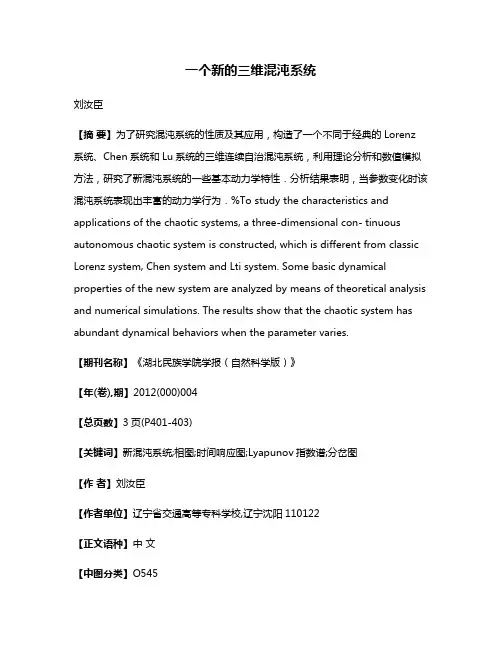
一个新的三维混沌系统刘汝臣【摘要】为了研究混沌系统的性质及其应用，构造了一个不同于经典的Lorenz 系统、Chen系统和Lu系统的三维连续自治混沌系统，利用理论分析和数值模拟方法，研究了新混沌系统的一些基本动力学特性．分析结果表明，当参数变化时该混沌系统表现出丰富的动力学行为．%To study the characteristics and applications of the chaotic systems, a three-dimensional con- tinuous autonomous chaotic system is constructed, which is different from classic Lorenz system, Chen system and Lti system. Some basic dynamical properties of the new system are analyzed by means of theoretical analysis and numerical simulations. The results show that the chaotic system has abundant dynamical behaviors when the parameter varies.【期刊名称】《湖北民族学院学报（自然科学版）》【年(卷),期】2012(000)004【总页数】3页(P401-403)【关键词】新混沌系统;相图;时间响应图;Lyapunov指数谱;分岔图【作者】刘汝臣【作者单位】辽宁省交通高等专科学校,辽宁沈阳110122【正文语种】中文【中图分类】O545由于混沌系统有1个正的Lyapunov指数，其动力学行为复杂，在非线性科学以及其他工程领域和社会科学领域得到了广泛的应用.自从1963年Lorenz［1］在分析气候数据时发现第一个混沌吸引子以来，后来人们称之为Lorenz系统.许多科研工作者对混沌的生成产生了浓厚的兴趣，不断地对Lorenz系统改进变形得到好多新的混沌系统［2－10］.这些新混沌系统的不断被发现，一方面丰富了混沌系统的数量，另一方面在混沌保密通讯方面以及控制和同步方面也有较广泛的应用.所以构造新的混沌系统是非常有好处的.本文通过计算机数值计算Lyapunov指数构造了一个新的混沌系统，通过一系列常规分析方法分析了系统的丰富的动力学行为.1 混沌模型及其混沌吸引子本文中所构造的新混沌系统数学模型为:这是一个非线性常微分方程组，其中x，y，z为系统的状态变量，a，b为系统的参数.当参数a=0.11，b=0.3时，利用 Wolf方法数值计算系统的三个 Lyapunov 指数为λ1=0.0647，λ2=－0.0023，λ3=－1.0331，说明此时系统处于混沌状态，图1给出了当参数a=0.11，b=0.3的混沌吸引子相图，轨线相互缠绕，动力学行为比较复杂.但目前轨线方程的计算还没有方法.2 新混沌系统的基本动力学分析2.1 时间响应对于非线性系统而言，从时间相应图上看状态值如果无规律的在一定范围内变化，说明系统可能在做混沌运动.图2给出了当参数a=0.11，b=0.3时系统的三个状态变量的时间响应图.图1 当参数a=0.11，b=0.3时系统的混沌吸引子 (a)xy平面;(b)xz平面;(c)yz平面Fig.1 Chaotic attractors of system when a=0.11，b=0.3(a)xy plane;(b)xz plane;(c)yz plane图2 系统的时间响应图(a)tx;(b)ty;(c)tzFig.2 Time responsedigram of the system(a)tx;(b)ty;(c)tz2.2 平衡点及其稳定性系统中当参数a=0.11，b=0.3时，令，可求得系统的2个平衡点分别为A(－0.5629，－0.5329，－0.0912)和 B(0.5329，0.5629，－0.1367).然后将系统线性化，将平衡点代入线性化矩阵得特征值都为不稳定的鞍焦点，当系统的平衡点不稳定时就会引发分岔与混沌现象，从而系统处于混沌状态.2.3 典型参数对系统运动状态的影响为了进一步研究系统参数变化时系统的运动变化情况.图3给出了固定参数b=0.3，系统随参数a∈［0，0.23］变化关于x的分岔图和Lyapunov指数谱图，几个典型参数下的周期轨如图4所示.图3 系统随参数a变化的分岔图和对应的Lyapunov指数谱图Fig.3 Bifurcation diagram and Lyapunov exponents spectrum of the system with parametera图4 系统在x－z平面的典型周期相图Fig.4 Typical cycle phase portraits of system in x－z plane图5给出了固定参数a=0.11，系统随参数b∈［0.1，0.3］变化关于x的分岔图和Lyapunov指数谱图，几个典型参数下的周期轨如图6所示.由这些图可见系统随参数变化表现出丰富的动力学行为，在混沌区域也有几处出现较窄的周期窗口. 图6 系统在x－z平面的典型周期相图Fig.6 Typical cycle phase portraits of system in x－zplane2.4 拓扑等价性由于本文构造的新混沌系统的混沌吸引子比较独特，与Lorenz吸引子形状完全不同，与Chen系统、Lü系统也不同，它们均有3个平衡点，而这个新系统只有2个平衡点，所以该新混沌系统与这3个混沌系统之间均不存在同胚变换，因此是一个新型的混沌系统.参考文献:［1］ Lorenz E N.Deterministic nonpefiodic flow［J］.At Mos Sci，1963，20(2):130－141.［2］ Chen G，Ueta T.Yet another chaotic attractor［J］.International Journal of Bifurcation and Chaos，1999，9(7):1465－1466.［3］Lü J.Chen G R.A new chaotic attractor cioned［J］.International Journal of Bifurcation and Chaos，2002，12(3):659－661.［4］Lü J，Chen G，Cheng D S.Celikovsky.Bridge the gap between the Lorenz system and the Chen system［J］.International Journal of Bifurcation and Chaos，2002，12(12):2917－2926.［5］高智中.一个新混沌系统［J］.湖南文理学院学报，2011，23(1):34－37. ［6］狄崇利，黄东卫，蔡为民.一类非线性系统的混沌特征分析［J］.天津师范大学学报，2010，30(2):1－5.［7］王杰智，陈增强，袁著祉.一个新的混沌系统及其性质研究［J］.物理学报，2006，55(8):3956－3963.［8］高智中.一个新自治混沌系统的动力学分析［J］.数值计算与计算机应用，2012，33(1):1－8.［9］韩春艳，薛华，吴新华.一个新的混沌模型及其数字伪随机信号的实现［J］.河北师范大学学报，2010，34(2):165－169.［10］张建雄，唐万生，徐勇.一个新的三维混沌系统［J］.物理学报，2008，57(11):6799－6809.。

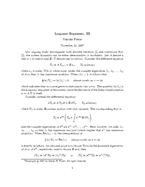
Lyapunov Exponents.IIISteven FinchNovember21,2007Our ongoing study encompasses both discrete iteration[1]and continuousflow [2];the system dynamics can be either deterministic or stochastic.Let A denote a real m×m matrix and B,X denote real m-vectors.Consider the difference equationX n=A X n−1+Bεn,X0arbitrarywhereεn is scalar N(0,1)white noise.Order the complex eigenvaluesλ1,λ2,...,λm of A so thatλ1has maximum modulus.When|λ1|>1,it follows that1ln|X n|→ln|λ1|>0almost surely as n→∞nwhich indicates that no convergence to stationarity can occur.The quantity ln|λ1|is the Lyapunov exponent of the system,since the derivative of the linear transformation x→A X is itself.Consider instead the differential equationdX t=A X t dt+B dW t,X0arbitrarywhere W t is scalar Brownian motion with unit variance.The correspondingflow isX t=e A t⎛⎝X0+t Z0e−A s B dW s⎞⎠and the complex eigenvalues of e A are eλ1,eλ2,...,eλm.Here,however,we orderλ1,λ2,...,λm so thatλ1has maximum real part(which implies that eλ1has maximum modulus).When Re(λ1)>0,the interpretation of1ln|Xt|→Re(λ1)almost surely as t→∞is exactly as before.An informal proof is to choose X0to be the dominant eigenvector of A or of e A,respectively,and to choose B=0;then|X n|=|A n X0|=|λ1|n|X0|or|X t|=|e A t X0|=|eλ1|t|X0|, 0Copyright c°2007by Steven R.Finch.All rights reserved.1respectively.See[3]for special treatment of the case m=1.The probability density ofln|X n|−n ln|λ1|,ln|X t|−t Re(λ1)is also of interest,and turns out to be doubly-exponential[3,4].Additive noise does not enter the formula for Lyapunov exponents;multiplicative noise contrasts in this regard.Let A,B denote real m×m matrices.The equations X n=A X n−1+B X n−1εn,X0arbitrary;dX t=A X t dt+B X t dW t,X0arbitraryrequire more intricate analysis.Let us focus only on the continuous-time case for now,leaving the discrete-time case for later.In the event A and B commute,that is,A B=B A,it can be proved that[5]X t=exp³³A−12B2´t+B W t´X0.There is,however,no consequential formula for the Lyapunov exponent that is valid for all m≥1and all A,B.Set m=1or m=2.Let us adhere to the convention of replacing A by A+1B2: dX t=³A+1B2´X t dt+B X t dW t,X0arbitrary.If m=1,A=a and B=σ>0,then the random variable ln|X t/X0|is normally distributed with mean a t and varianceσ2t(the process X t is often called geometric Brownian motion).Clearly1ln|Xt|→a almost surely as t→∞.Stability is unchanged by noise in this example.The same can be said if m=2,A=Ãa00b!and B=Ãσ00σ!where a>b andσ>0.If insteadB=Ã0−σσ0!then it can be proved that[6,7]1 t ln|X t|→12(a+b)+12(a−b)I1³a−b2´I0³a−b2´almost surelywhere I0,I1are modified Bessel functions[8].For example,when a=1,b=−2and σ=10,the Lyapunov exponent has value−0.4887503163...[9].For the same a and b,the Lyapunov exponent has value0.3941998582...whenσ=1,and is zero precisely whenσ=1.4560286969...[6].More noise implies enhanced stability in this example.If instead[10,11]A=Ã0100!and B=Ã00σ0!then1tln|X t|→κσ2/3=(0.2893082598...)σ2/3almost surelyandκ=π121/6Γ(1/3)2=31/3√π22/3Γ(1/6).What happens when the bottom row of A is nonzero?IfA=Ã01−α2β!and B=Ã00σ0!whereβ2>α,then more complicated formulation emerges.We avoid the hypergeo-metric functions in[12,13],preferring modified Bessel functions(of both integer and fractional types).Letγ=σ22,δ=4(β2−α)9γ2for convenience.Definef(α,β,γ)=32π3∞Z√z expµ−112γ2z3+³β2−α´z¶dz=δ1I−23³√´I−13³√´γ+2³2´1δ1I13³√´2(β2−α)γ1+δ1I13³√´I23³√´γ+ 6³2´2γ1δ2I23³√´2(β2−α)2+2³2´2(β2−α)δ1I13³√´I43³√´γ5+ 2³2´1(β2−α)1δ1I23³√´I53³√´γ43,g(α,β,γ)=32π3∞Z1√z expµ−112γ2z3+³β2−α´z¶dz=³23´13δ1µI−1³√´2+I−1³√´I1³√´+I1³√´2¶γ1=3ÃAiµ³3´2δ13¶2+Biµ³3´2δ13¶2!2γ1then1ln|Xt|→β+γ2f(α,β,γ)g(α,β,γ)almost surely.For example,whenα=1and|β|>1isfixed,the Lyapunov exponent is decreasing as a function ofγ∈(0,(β2−1)3/2γ0)and increasing forγ∈((β2−1)3/2γ0,∞),where γ0=1.6946141069....At criticality,we havef(1,β,(β2−1)3/2γ0) g(1,β,(β2−1)3/2γ0)=1(β2−1)γ0(1.4567743021...)=2(β2−1)γ0(1+0.8848441574...)−1/2;further stabilization by noise beyond this point is impossible.As another example, whenα=1andγ>0isfixed,we havelim |β|→1+f(1,β,γ)g(1,β,γ)=Ã4γ!2/3κ=2γκσ2/3,consistent with preceding zero-row results.The constantκ=0.2893082598...also appears in[14],but reasons for this connection are unclear.Explicit expressions like the above are quite rare in this area.We hope to report later on[15],which seems to present a promising approach but unfortunately gives no examples.References[1]S.R.Finch,Lyapunov exponents,unpublished note(2007).[2]S.R.Finch,Lyapunov exponents.II,unpublished note(2007).[3]S.R.Finch,Another look at AR(1),arXiv:0710.5419.[4]S.R.Finch,Extreme value constants,Mathematical Constants,Cambridge Univ.Press,2003,pp.363—367.[5]L.Arnold,Stochastic Differential Equations:Theory and Applications,Wiley,1974,pp.125—144,176—201;MR0443083(56#1456)[6]P.H.Baxendale,Moment stability and large deviations for linear stochasticdifferential equations,Probabilistic Methods in Mathematical Physics,Proc.1985 Katata/Kyoto conf.,ed.K.Itˆo and N.Ikeda,Academic Press,1987,pp.31—54;MR0933817(89c:60068).[7]P.E.Kloeden and E.Platen,Numerical Solution of Stochastic Differential Equa-tions,Springer-Verlag,1992,pp.103—126,148—152,232—241,396—399,540—548;MR1214374(94b:60069).[8]M.Abramowitz and I.A.Stegun,Handbook of Mathematical Functions,Dover,1972,pp.374—377;MR1225604(94b:00012).[9]D.Talay,Approximation of upper Lyapunov exponents of bilinear stochasticdifferential systems,SIAM J.Numer.Anal.28(1991)1141—1164;MR1111458 (92i:60119).[10]S.T.Ariaratnam and W.C.Xie,Lyapunov exponent and rotation number of atwo-dimensional nilpotent stochastic system,Dynam.Stability Systems5(1990) 1—9;MR1057870(91h:60086).[11]W.C.Xie,Lyapunov exponents and moment Lyapunov exponents of a two-dimensional near-nilpotent system,Trans.ASME J.Appl.Mech.68(2001)453—461;MR1836484.[12]P.Imkeller and C.Lederer,An explicit description of the Lyapunov exponentsof the noisy damped harmonic oscillator,Dynam.Stability Systems14(1999) 385—405;MR1746113(2000m:34122).[13]P.Imkeller and C.Lederer,Some formulas for Lyapunov exponents and rotationnumbers in two dimensions and the stability of the harmonic oscillator and the inverted pendulum,Dyn.Syst.16(2001)29—61;MR1835906(2002j:60100). [14]B.Derrida and E.Gardner,Lyapounov exponent of the one-dimensional An-derson model:weak disorder expansions,J.Physique45(1984)1283—1295;MR0763431(85m:82098).[15]A.Leizarowitz,Exact results for the Lyapunov exponents of certain linear Itosystems,SIAM J.Appl.Math.50(1990)1156—1165;MR1053924(91j:93120).。

a r X i v :c o n d -m a t /0407730v 1 [c o n d -m a t .s t a t -m e c h ] 28 J u l 2004On some common misconceptions regarding the ”Ergodic Hierarchy”.Henk van BeijerenInstitute for Theoretical PhysicsUtrecht UniversityLeuvenlaan 4,3584CE Utrecht,The Netherlands(Dated:February 6,2008)The well-known ergodic hierarchy of sheerly ergodic,mixing,Kolmogorov and Bernoulli systems,with each next level supposedly encompassing the previous one,is shown to be too simplistic in itsusual formulation.A K-system can be sheerly ergodic and sometimes may be reduced to a sheerlymixing system by some simple projection.More precise characterizations of ergodic properties ofdynamical systems should start out from a consideration of the full Lyapunov spectrum.I.INTRODUCTION In ergodic theory it has been common to define a hierarchy of degrees of ergodicity [1].The weakest property is sheer ergodicity .This implies that,under some given dynamics,the time average of any Lebesgue integrable function on phase space equals an average over some properly chosen subset S of phase space.If the dynamics leaves volumes in phase space unchanged,as is the case for Hamiltonian dynamics,this phase space average simply assigns weights proportional to phase space volume to various parts of this subset.If the dynamics is phase space contracting one has to choose an attractor as subset and use the SRB-measure for its weighting,i.e.each part of the subset has to be weighted by its asymptotic phase space contraction factor.The next property in the ergodic hierarchy is mixing .This implies that under the dynamics the image of any subset A of non-zero measure becomes uniformly distributed on S ,i.e.the measure of its intersection with an arbitrary other subset B of non-zero measure approaches µ(A )µ(B )/µ(S )as time increases.Mixing implies ergodicity,but not the other way around;therefore mixing is a stronger property than sheer ergodicity.In fact one may distinguish between strong mixing ,where the uniformity property holds pointwise in time,and weak mixing where it only holds on average over long stretches of time.The next property in the ergodic hierarchy is that of being a Kolmogorov system or K-system.The original definition of this is rather involved,but for my present purposes it suffices that K-systems are systems with positive Kolmogorov-Sinai entropy (or KS-entropy).For systems without escape,i.e.with dynamics mapping all points of S onto S ,according to Pesin’s theorem this is equivalent to the requirement that the system has at least one positive Lyapunov exponent,or in other words,is chaotic.It is commonly assumed that being a K-system implies mixing and therefore is a stronger property.An even stronger property,the strongest in the ergodic hierarchy,is for a system being a Bernoulli system.This is most easily defined for maps,rather than flows (for the latter one therefore may take recourse to time slices or to Poincar´e maps).It implies that S may be decomposed into a discrete collection of subsets A i with the following property:for any subset of all points on S with a given history,i.e.with a given sequence i −1,i −2,···of subsets visited at previous mappings,the fraction of points ending up in A i at the next mapping is simply proportional to the measure of this subset.In other words,without additional information on where the phase point is or came from,the outcome of the mapping is like determined by pure chance,irrespective of what happened before.Here I will argue that in fact this hierarchy should not be taken too litterally.A K-system may be non-mixing and even if it is mixing,its ergodic behavior in certain respects need not be stronger than that of a merely mixing system.II.MIXED BEHA VIORS A standard example of a map exhibiting the Bernoulli property is the baker map,defined on the unit square as B (x,y )=(2x mod 1,y/2+int (2x )),(1)with int (x )the integer part of x .This map is area conserving and has Lyapunov exponents ±log 2,with corresponding eigenvectors in tangent space (1,0)and (0,1).It satisfies a Bernoulli scheme with respect to the subdivision of the unit square into the two subsets 0≤x <1/2and 1/2≤x <1.It may be extended to a map on the unit cube of the formM (x,y,z )=(2x mod 1,y/2+int (2x ),f (z )),(2)with f (z )mapping the unit interval onto itself.This map is still Bernoulli,as it still satisfies a Bernoulli scheme with respect to the subdivision,now of the unit cube,into the subsets 0≤x <1/2and 1/2≤x <1.It still has a2 Lyapunov exponent log2,so it obviously is still a K-system,but whether it is mixing depends on the nature of the function f.If f is merely ergodic,e.g.a shift mod1over an irrational numberα,the map M is not mixing.So the statement that the property of being a K-system implies mixing,obviously is not true.In this case one may say that M combines the property of being Bernoulli when projected on the x−y plane,with that of being merely ergodic when projected on the z-axis.Therefore,to me it also seems dubious to state in general that K-systems are more strongly ergodic than mixing systems.In the present example I would say that the system is no more ergodic than the one defined by the one-dimensional mapping f alone.One may object now that the present example is very atypical because it can be factorized into a two-dimensional mapping that is Bernoulli and a one-dimensional mapping that is merely ergodic.It is not hard though to extend this example into non-factorizable mappings,e.g.M1(x,y,z)=(2x+z mod1,y/2+int(2x),z+α+(2x+z mod1)+y/2+int(2x)−x−y),(3) which acts like a shift map to which an x and y dependent constant is added.Going to higher dimensions one may,for example in d=4,devise mappings that asymptotically reduce to a baker map in the x−y plane times a quasi-periodic map on some curve in the remaining coordinates.In this case the decoupling of the two maps may easily be designed to hold only asymptotically on the attractor.No doubt increasingly more complicated scenario’s may be designed with increasing dimensionality.III.DISCUSSIONFor the general case of a mapping orflow in a high-dimensional phase space the ergodic properties of the dynamics on a given ergodic component willfirst of all depend on the spectrum of Lyapunov exponents.For simplicity,let us restrict ourself to symplectic maps orflows,for which the spectrum is odd(a Lyapunov exponentλalways comes together with−λ).Then,if there are no zero exponents,in the case of maps,or,in the case offlows,just a single pair related to displacements in the direction of theflow,one may say the system fully has the character of a K-system. No projections are possible in directions where the dynamics is merely mixing or even merely ergodic.Whether the system is also Bernoulli is a separate problem that has to be decided case by case.If there are more zero Lyapunov exponents,one should decidefirst of all what is the character of the behavior of the dynamics in the corresponding directions.This may be hard to decide,especially if the dynamics in these directions cannot be decoupled from that in the remaining ones.Without further specifications the usual ergodic hierarchy remains a qualitative characterization of increasingly randomizing and chaotic types of dynamics.As such it is extremely useful.But forfixing a rigorous sequence in which each next stage implies the previous one,obviously more precision is needed.AcknowledgmentsHvB acknowledges support by the Mathematical physics program of FOM and NWO/GBE.[1]V.I.Arnol’d and A.Avez,Ergodic Problems of Clasical Mechanics,(W.A.Benjamin,New york,1968)。

A new test for chaosin deterministic systemsBy Georg A.Gottwald†and Ian Melbourne‡We describe a new test for determining whether a given deterministic dynamical system is chaotic or nonchaotic.In contrast to the usual method of computing the maximal Lyapunov exponent,our method is applied directly to the time series data and does not require phase space reconstruction.Moreover,the dimension of the dynamical system and the form of the underlying equations is irrelevant.The input is the time series data and the output is0or1depending on whether the dynamics is non-chaotic or chaotic.The test is universally applicable to any deterministic dynamical system,in particular to ordinary and partial differential equations,and to maps.Our diagnostic is the real valued function p(t)= t0φ(x(s))cos(θ(s))d s whereφis an observable on the underlying dynamics x(t)andθ(t)=ct+ t0φ(x(s))d s.The constant c>0isfixed arbitrarily.We define the mean-square-displacement M(t) for p(t)and set K=lim t→∞log M(t)/log ing recent developments in ergodic theory,we argue that typically K=0signifying nonchaotic dynamics or K=1 signifying chaotic dynamics.Keywords:Chaos,deterministic dynamical systems,Lyapunov exponents,mean square displacement,Euclidean extension1.IntroductionThe usual test of whether a deterministic dynamical system is chaotic or nonchaotic is the calculation of the largest Lyapunov exponentλ.A positive largest Lyapunov exponent indicates chaos:ifλ>0,then nearby trajectories separate exponentially and ifλ<0,then nearby trajectories stay close to each other.This approach has been widely used for dynamical systems whose equations are known(Abarbanel et al.1993;Eckmann et al.1986;Parker&Chua1989).If the equations are not known or one wishes to examine experimental data,this approach is not directly applicable. However Lyapunov exponents may be estimated(Wolf et al.1985;Sana&Sawada 1985;Eckmann et al.1986;Abarbanel et al.1993)by using the embedding theory of Takens(1981)or by approximating the linearisation of the evolution operator. Nevertheless,the computation of Lyapunov exponents is greatly facilitated if the underlying equations are known and are low-dimensional.In this article,we propose a new0–1test for chaos which does not rely on knowing the underlying equations,and for which the dimension of the equations is irrelevant.The input is the time series data and the output is either a0or a1 depending on whether the dynamics is nonchaotic or chaotic.Since our method is †School of Mathematics and Statistics,University of Sydney,NSW2006,Australia‡Department of Mathematics and Statistics,University of Surrey,Guildford,Surrey GU27XH, UKArticle submitted to Royal Society T E X Paper2G.Gottwald and I.Melbourneapplied directly to the time series data,the only difference in difficulty between analysing a system of partial differential equations or a low-dimensional system of ordinary differential equations is the effort required to generate sufficient data.(As with all approaches,our method is impracticable if there are extremely long tran-sients or once the dimension of the attractor becomes too large.)With experimental data,there is the additional effect of noise to be taken into consideration.We briefly discuss this important issue at at the end of this paper.However,our aim in this paper is to present ourfindings in the situation of noise-free deterministic data.2.Description of the0–1test for chaosTo describe the new test for chaos,we concentrate on the continuous time case and denote a solution of the underlying system by x(t).The discrete time case is handled analogously with the obvious modifications.Consider an observableφ(x) of the underlying dynamics.The method is essentially independent of the actual form ofφ—almost any choice ofφwill suffice.For example if x=(x1,x2,...,x n) thenφ(x)=x1is a possible and simple choice.Choose c>0arbitrarily and defineθ(t)=ct+ t0φ(x(s))d s,p(t)= t0φ(x(s))cos(θ(s))d s.(2.1)(Throughout the examples in§3and§4wefix c=1.7once and for all.)We claim that(i)p(t)is bounded if the underlying dynamics is nonchaotic and(ii)p(t)behaves asymptotically like a Brownian motion if the underlying dynam-ics is chaotic.The definition of p in(2.1),which involves only the observableφ(x),highlights the universality of the test.The origin and nature of the data which is fed into the system(2.1)is irrelevant for the test,and so is the dimension of the underlying dynamics.Later on,we briefly explain the justification behind the claims(i)and(ii).For the moment,we suppose that the claims are correct and show how to proceed.To characterise the growth of the function p(t)defined in(2.1),it is natural to look at the mean square displacement(MSD)of p(t),defined to be1M(t)=limT→∞A new test for chaos3 which obviously does not change the slope K.)This allows for a clear distinction of a nonchaotic and a chaotic system as K may only take values K=0or K=1. We have lost though the possibility of quantifying the chaos by the magnitude of the largest Lyapunov exponentλ.Numerically one has to make sure that initial transients have died out so that the trajectories are on(or close to)the attractor at time zero,and that the integration time T is long enough to ensure T t.3.An example:the forced van der Pol oscillatorWe illustrate the0–1test for chaos with the help of a concrete example,the forced van der Pol system,˙x1=x2˙x2=−d(x21−1)x2−x1+a cosωt(3.1) which has been widely studied in nonlinear dynamics(van der Pol1927;Guck-enheimer&Holmes1990).Forfixed a and d,the dynamics may be chaotic or nonchaotic depending on the parameterω.Following Parlitz&Lauterborn(1987), we take a=d=5and letωvary from2.457to2.466in increments of0.00001. Chooseφ(x)=x1+x2and c=1.7.We stress that the results are independent of these choices for all practical purposes.As described below in§5,almost all choices will work.(Deliberately poor choices such as c=0,orφ=7orφ=t obviously fail;sensible choices that fail are virtually impossible tofind.)Infigure1we show a plot of K versusω.The periodic windows are clearly seen. As a comparison we show infigure2the largest Lyapunov exponentλversusω. Since the onset of chaos does not occur until afterω=2.462we display the results only for the range2.462<ω<2.466infigures1and2.(Both methods easily indicate regular dynamics for2.457<ω<2.462.)Naturally we do not obtain the values K=0and K=1exactly–the mathe-matical results that underpin our method predict these values in the limit of infi-nite integration time.(The same caveat applies equally to the Lyapunov exponent method.)In producing the data forfigures1and2,we allowed for a transient of 200,000units of time and then integrated up to time T=2,000,000.As can be seen infigure3,for most of the400data points in the range ofω,we obtain K>0.8or K<0.01.Next,we carry out the0–1test for the forced van der Pol system in the situation of a more limited quantity of data.The results are shown infigure4for2.463<ω<2.465.We again allow for a transient time200,000but then integrate only for T=50,000.The transitions between chaotic dynamics and periodic windows are almost as clear with T=50,000as they are with T=2,000,000even though the convergence of K to0or1is better with T=2,000,000.Article submitted to Royal Society4G.Gottwald and I.Melbourne 00.20.40.60.811.22.462 2.463 2.464 2.465 2.466Figure 1.Asymptotic growth rate K of the mean square displacement (2.2)versus ωfor the van der Pol system (3.1)determined by a numerical simulation of the skew product system (3.1)and (2.1)with a =d =5,c =1.7,φ(x )=x 1+x 2and ωvarying from 2.462to 2.466.The integration interval is T =2,000,000after an initial transient of 200,000units of time.-0.1-0.08-0.06-0.04-0.020.020.040.060.080.12.462 2.463 2.464 2.465 2.466Figure rgest Lyapunov exponent λversus ωfor the van der Pol system (3.1)with a =d =5and ωvarying from 2.462to 2.466(cf Parlitz &Lauterborn 1987).The integration interval is T =2,000,000after an initial transient of 200,000units of time.Article submitted to Royal SocietyA new test for chaos 500.20.40.60.811.22.462 2.463 2.464 2.465 2.466Figure 3.Asymptotic growth rate K versus ωfor the van der Pol system (3.1)as in figure 1with T =2,000,000.The horizontal lines represent K =0.01and K =0.8.0.20.40.60.811.22.463 2.464 2.46500.20.40.60.811.22.463 2.464 2.465Figure 4.Asymptotic growth rate K versus ωvarying from 2.463to 2.465for the van der Pol system as in figures 1and 3but with integration interval T =50,000after an initial transient of 200,000units of time.The horizontal lines represent K =0.01and K =0.8.Article submitted to Royal Society6G.Gottwald and I.Melbourne4.Further examplesTo test the method on high-dimensional systems we investigated the driven and damped Kortweg-de Vries(KdV)equation(Kawahara&Toh1988)u t+uu x+βu xxx+αu xx+νu xxxx=0,(4.1) on the interval[0,40]with periodic boundary conditions.This partial differential equation has non-chaotic solutions if the dispersionβis large and exhibits spatio-temporal chaos for sufficiently smallβ.Note that equation(4.1)reduces to the KdV equation whenα=ν=0,and reduces to the Kuramoto-Sivashinksy equation whenβ=0.Wefixα=2,ν=0.1and varyβ.Forβ=0,it is expected that the dynamics of the Kuramoto-Sivashinksy equation are chaotic for these parameter values.As an observable we usedφ(u(x,t))=u(x0,t)where x0is an arbitrarilyfixed position, and we iterated until time T=35,000.The0–1test confirms that the dynamics is chaotic atβ=0(with K=0.939).Also,we obtain K=0.989atβ=0.1and K=0.034atβ=4,indicating chaotic and regular dynamics respectively at these two parameter values.Finally,for discrete dynamical systems,we tried out the test with an ecological model whose chaotic component is coupled with strong periodicity(Brahona& Poon1996;Cazelles&Ferriere1992).The modelx k+1=118y k exp(−0.001(x k+y k))y k+1=0.2x k exp(−0.07(x k+y k))+0.8y k exp(−0.05(0.5x k+y k))has a non-connected chaotic attractor consisting of seven connected components. Our test yields K=1.023with only10,000data points and clearly shows that the dynamics is chaotic.5.Justification of the0–1test for chaosThe function p(t)can be viewed as a component of the solution to the skew product system˙θ=c+φ(x(t))˙p=φ(x(t))cosθ(5.1)˙q=φ(x(t))sinθdriven by the dynamics of the observableφ(x(t)).Here(θ,p,q)represent coordinates on the Euclidean group E(2)of rotationsθand translations(p,q)in the plane.We note that inspection of the dynamics of the(p,q)-trajectories of the group extension provides very quickly(for small T)a simple visual test of whether the underlying dynamics is chaotic or nonchaotic as can be seen fromfigure5.Article submitted to Royal SocietyA new test for chaos7(a)(b)Figure5.The dynamics of the translation components(p,q)of the E(2)-extension(5.1) for the van der Pol system(3.1)with a=d=5,c=1.7,φ(x)=x1+x2.These plots were obtained by integrating for T∼1400(with timestep0.01).In(a),an unbounded trajectory is shown corresponding to chaotic dynamics atω=2.46550.In(b),a bounded trajectory is shown corresponding to regular dynamics atω=2.46551.Article submitted to Royal Society8G.Gottwald and I.MelbourneIn Nicol et al.(2001)it has been shown that typically the dynamics on the group extension is sublinear and furthermore that typically the dynamics is bounded if the underlying dynamics is nonchaotic and unbounded(but sublinear)if the underlying dynamics is chaotic.Moreover,the p and q components each behave like a Brownian motion on the line if the chaotic attractor is uniformly hyperbolic(Field et al. 2002).A nondegeneracy result of Nicol et al.(2001)ensures that the variance of the Brownian motion is nonzero for almost all choices of observableφ.Recent work of Melbourne&Nicol(2002)indicates that these statements remain valid for large classes of nonuniformly hyperbolic systems,such as H´e non-like attractors.There is a weaker condition on the‘chaoticity’of X that guarantees the desired growth rate K=1for the mean square displacement(2.2):namely that the autocor-relation function ofφ(x)cos(θ)decays at a rate that is better than quadratic.More precisely,let x(t)andθ(t)denote solutions to the skew product equations(5.1)with initial conditions x0andθ0respectively.If there are constants C>0andα>2 such thatφ(x(t))cos(θ(t))φ(x0)cosθ0d x0dθ0 ≤Ct−α,for all t>0,then K=1as desired(Biktashev&Holden1998;Ashwin et al.2001; Field et al.2002).(Again,results of Nicol et al.(2001);Field et al.(2002);and Melbourne&Nicol(2002)ensure that the appropriate nondegeneracy condition holds for almost all choices ofφ.)There is a vast literature on proving decay of correlations(Baladi1999)and this has been generalised to the equivariant setting for discrete time by Field et al.(2002)and Melbourne&Nicol(2002)and for continuous time by Melbourne&T¨o r¨o k(2002).It follows from these references that K=1,for large classes of chaotic dynamical systems.One might ask why it is not better to work,instead of the E(2)-extension,with the simpler R-extension˙p=φ(x(t).In principle,p(t)can again be used as a detector for chaos.However,by the ergodic theorem p(t)will typically grow linearly with rate equal to the space average of φ.This would lead to K=2irrespective of whether the dynamics is regular or chaotic.Hence,it is necessary to subtract offthe linear term of p(t)in order to observe the bounded/diffusive growth that distinguishes between regular/chaotic dynamics.Subtracting this linear term is a highly nontrivial numerical obstruc-tion.The inclusion of theθvariable in the definition(2.1)of p(t)and in the skew product(5.1)kills offthe linear term.6.DiscussionWe have established a simple,inexpensive,and novel0–1test for chaos.The com-putational effort is of low cost,both in terms of programming efforts and in terms of actual computation time.The test is a binary test in the sense that it can only distinguish between nonchaotic and chaotic dynamics.This distinction is extremely clear by means of the diagnostic variable K which has values either close to0or close to1.The most powerful aspect of our method is that it is independent of the nature of the vectorfield(or data)under consideration.In particular the equationsArticle submitted to Royal SocietyA new test for chaos9 of the underlying dynamical system do not need to be known,and there is no prac-tical restriction on the dimension of the underlying vectorfield.In addition,our method applies to the observableφ(x(t))rather than the full trajectory x(t).Related ideas(though not with the aim to detect chaos)have been used for PDE’s in the context of demonstrating hypermeander of spirals in excitable me-dia(Biktashev&Holden1998)where the spiral tip appears to undergo a planar Brownian motion(see also Ashwin et al.2001).We note also the work of Coullet &Emilsson(1996)who studied the dynamics of Ising walls on a line,where the motion is the superposition of a linear drift and Brownian motion.(This is an ex-ample of an R-extension which we mentioned briefly in§5.As we pointed out then, the linear drift is an obstruction to using an R-extension to detect chaos.) From a purely computational point of view,the method presented here has a number of advantages over the conventional methods using Lyapunov exponents. At a more technical level,we note that the computation of Lyapunov exponents can be thought of abstractly as the study of the GL(n)-extension˙A=(d f)Ax(t)where GL(n)is the space of n×n matrices,A∈GL(n),and n is the size of the system.Note that the extension involves n2additional equations and is defined us-ing the linearisation of the dynamical system.To compute the dominant exponent, it is still necessary to add n additional equations,again governed by the linearised system.In contrast,our method requires the addition of two equations.In this paper,we have concentrated primarily on the idealised situation where there is an in principle unlimited amount of noise-free data.However,in§3we also demonstrated the effectiveness of our method for limited data sets.An issue which will be pursued in further work is the effect of noise which is inevitably present in all experimental time series.Preliminary results show that our test can cope with small amounts of noise without difficulty.A careful study of this capability,and comparison with other methods,is presently in progress.We are grateful to Philip Aston,Charlie Macaskill and Trevor Sweeting for helpful dis-cussions and suggestions.The research of GG was supported in part by the European Commission funding for the Research Training Network“Mechanics and Symmetry in Europe”(MASIE).ReferencesAbarbanel H.D.I.,Brown R.,Sidorovich J.J.&Tsimring L.S.1993The analysis of observed chaotic data in physical systems.Rev.Mod.Phys.65,1331–1392.Ashwin P.,Melbourne I.&Nicol M.2001Hypermeander of spirals;local bifurcations and statistical properties.Physica D14,275–300.Baladi V.1999Decay of correlations.In Smooth Ergodic Theory and its Applications, Amer.Maths.Soc.297–325.Biktashev V.N.&Holden.A.V.2001Deterministic Brownian motion in the hyperme-ander of spiral waves.Physica D116,342–382.Brahona M.&Poon C.-S.1996Detection of nonlinear dynamics in short,noisy time series.Nature381,215–217.Cazelles B.&Ferriere R.H.1992How predictable is chaos?Nature355,25–26.Article submitted to Royal Society10G.Gottwald and I.MelbourneCoullet P.&Emilsson K.1996Chaotically induced defect diffusion.In:Instabilities and Nonequilibrium Structures,V(ed.E.Tirapegui and W.Zeller),pp.55–62.Dordrecht: Kluwer.Eckmann J.-P.,Kamphurst S.O.,Ruelle D.&Ciliberto S.1986Liapunov exponents from time series.Phys.Rev.A34,4971–4979.Field M.,Melbourne I.&T¨o r¨o k A.2002Decay of correlations,central limit theorems and approximation by Brownian motion for compact Lie group extensions.Ergod.Th.& Dynam.Sys.To appear.Guckenheimer J.&Holmes P.1990Nonlinear Oscillations,Dynamical Systems,and Bi-furcations of Vector Fields.Appl.Math.Sci.42,New York:Springer.Kawahara T.&Toh S.1988Pulse interactions in an unstable disspative-dispersive non-linear system.Phys.Fluids31,2103–2111.Melbourne I.&Nicol M.2002Statistical properties of endomorphisms and compact group extensions.Preprint,University of Surrey.Melbourne I.&T¨o r¨o k A.2002Central limit theorems and invariance principles for time-one maps of hyperbolicflmun.Math.Physics229,57–71.Nicol M.,Melbourne I.&Ashwin P.2001Euclidean extensions of dynamical systems.Nonlinearity14,275–300.Parker T.S.&Chua L.O.1989Practical Numerical Algorithms for Chaotic Systems.New York:Springer.Parlitz U.&Lauterborn W.1987Period-doubling cascades and devil’s staircases of the driven van der Pol oscillator.Phys.Rev.A36,1428–1434.Press W.H.,Teukolsky S.A.,Vetterling W.T.&Flannery B.P.1992Numerical Recipes in C.Cambridge University Press.Sano M.&Sawada Y.1985Measurement of the Lyapunov spectrum from a chaotic time series.Phys.Rev.Lett.55,1082–1085.Takens F.1981Detecting strange attractors in turbulence.Lecture Notes in Mathematics 898,366–381,Berlin:Springer.van der Pol B.1927Forced oscillations in a circuit with nonlinear resistance(receptance with reactive triode).Philos Mag.43,700.Wolf A.,Swift J.B.,Swinney H.L.&Vastano J.A.1985Determining Lyapunov exponents from a time series.Physica D16,285–317.Article submitted to Royal Society。

With y y x x R J R J 1,1== and ()y x y x x yk k k J k J Q −+=22, the coefficients i a in the equation (9’) are:()()()()y x y x x y y x y x y x y x y x k k k J k J k k J J J J J J Q k k g a +−−+−++−=2222209991418()()()()(()()()()()())y y x x y x y x x y y x y x y x y x x y y x y x y x y x x y y x y x x y y x y x x y y x y y x x y x k J k J k k k J k J k k J J k k k J k J J J k k J J k J k J J J k J k J J J k J k J J J k J k J J J Q g a ++++++−+−+−+−−+++++=593576286332323223322222/31()()()(()()()())y x y x x y y x y x x y y x y x y x y x y x x y y x y x y x k k k k k J k J k J k J k k J J J J k k k J k J J J k k J J Q g a +++++−−−+−+++=4422222222222330141813()()()()()x y y x y x y x y x x y y x k J k J J J k k k J k J J J Q g a 332/13233+++−+=14=a1. Lord Rayleigh, “Investigations of the character of the equilibrium of an incompressible heavy fluid of variable density” Proc.Lond.Math.Soc. 14, 170 (1883)2. R.M.Davies, G.I.Taylor, “The mechanics of large bubbles rising through extended liquids and through liquids in tubes” Proc.Roy.Soc. A200, 375 (1950)3. D.H.Sharp, “An overview of Rayleigh-Taylor instability” Physica D 12, 3 19844. S.Chandrasekhar, Hydrodynamic and hydromagnetic stability, 3d ed. (Dover Publications Inc., New York, 1981), pp.428-477; K.O.Mikaelian, “Effect of viscosity on Rayleigh-Taylor and Richtmeyer-Meshkov instabilities” Phys.Rev.E 47, 375 (1993)5. K.I.Read, “Experimental investigation of turbulent mixing by Rayleigh-Taylor instability” Physica D 12, 45 (1984); Yu.A.Kucherenko at al, “Experimental study into the asymptotic stage of separation of the turbulized mixtures in gravitationally stable mode” Laser Part. Beams 15, 17 (1997); Izv. Akad. Nauk SSSR, Mekh. Zhidk. Gaza 6, 157 (1978)6. G.Dimonte M.Schneider, “Density ratio dependence of Rayleigh-Taylor mixing for sustained and impulsive acceleration histories” Phys.Fluids 12, 304 (2000);M.Schneider, G.Dimonte, B.Remington, “Large and small scale structures in Rayleigh-Taylor mixing” Phys.Rev.Lett. 80, 3507 (1998)7. F.H.Harlow, J.E.Welch, “Numerical study of large-amplitude free-surface motion” Phys.Fluids 9,842 (1966); D.L.Youngs, “Numerical simulations of turbulent mixing by Rayleigh-Taylor instability” Physica D 12, 32, (1984); R.Menikoff, C.Zemach,“Rayleigh-Taylor instability and the use of conformal maps for ideal fluid flow”p.Phys. 51, 28 (1983); G.R.Baker, D.I.Meiron, S.A.Orszag, “Vortexsimulations of the Rayleigh-Taylor instability” Phys.Fluids 23, 1485 (1980); G.Gardner, J.Glimm, O.McBryan, R.Menikoff, D.H.Sharp, Q.Zhang, “The dynamics of bubble growth for Rayleigh-Taylor instability” Phys.Fluids 31, 447 (1988)8. X.L.Li, “Study of three-dimensional Rayleigh-Taylor instability” Phys.FluidsA5, 1904 (1993); X.L.Li, “A numerical study of three-dimensional bubble merger in the Rayleigh-Taylor instability” Phys.Fluids 8, 336 (1996)9. D.L.Youngs, “Three-dimensional numerical simulations of turbulent mixing by Rayleigh-Taylor instability” Phys.Fluids A 3, 1312 (1991)10. U.Alon, J.Hecht, D.Offer, D.Sharts, “Power-laws and similarity of Rayleigh-Taylor and Richtmyer-Meshkov mixing fronts at all density ratios” Phys.Rev.Lett.74, 534 (1995)11. S.I.Abarzhi, “Stable steady flows in Rayleigh-Taylor instability”Phys.Rev.Lett.89, 1332 (1998); “Non-linear three-dimensional Rayleigh-Taylor instability” Phys.Rev.E, 59, 1729 (1999)12. A.V.Shubnikov and V.A.Koptsik, Symmetry in science and art, Plenum New York, 197413. yzer, “On the instability of superposed fluids in a gravitational field”Astrophys.Jour. 122, 1 (1955); P.R.Garabedian, “On steady-state bubbles generated by Taylor instability” Proc.Roy.Soc. A241, 423 (1957)14. S.I.Abarzhi, “The stationary spatially periodic flows in Rayleigh-Taylor instability: solutions multitude and its dimension” Physica Scripta T66, 238 (1996);“Stationary solutions of the Rayleigh-Taylor instability for spatially periodic flows:questions of uniqueness, dimensionality and universality” Zh.Eksp.Teor.Fiz. 110,1841 (1996) (Sov.Phys.JETP 83, 1012)15. S.I.Abarzhi and N.A.Inogamov, “Stationary solutions in the Rayleigh-Taylor instability for spatially periodic flow” Zh.Eksp.Teor.Fiz. 107,245 (1995) (Sov.Phys.JETP 80,132 (1995)); N.A.Inogamov, “Stationary solutions in the theory of the hydrodynamic Rayleigh-Taylor instability” Pis’ma Zh.Eksp.Teor.Fiz. 55, 505 (1992) (Sov.Phys.JETP Lett. 55, 521 (1992))16. A.Oparin, “Numerical simulations of Rayleigh-Taylor instability using quasi-monotonic grid-characteristic approach” private communication, 1998; M.F.Ivanov,A.M.Oparin, V.G.Sultanov, V.E.Fortov, “Certain features of development of the Rayleigh-Taylor instability in 3D geometry” Doklady Physics 44, 491 (1999) (Doklady Akademii Nauk 367, 464 (1999))17. R.J.Taylor, J.P.Dahlburg, A.Iwase, J.J.Gardner, D.E.Fyfe O.Willi,“Measurement and Simulation of Laser Imprinting and Consequent Rayleigh-Taylor growth” Phys.Rev.Lett.76, 1643 (1996); M.M.Marinak, S.G.Gledinning, R.J.Wallace, B.A.Remington, et al, “Non-linear evolution of a three-dimensional multimode perturbation” Phy.Rev.Lett. 80, 4426 (1998);18. Dalziel SB, Linden PF, Youngs DL, “Self-similarity and internal structure of turbulence induced by Rayleigh-Taylor instability” Jour.Fluid Mechanics, 399, 1 (1999)19. V.E.Zakharov, “Stability of periodic waves of finite amplitude on deep fluid surface” Prikl.Mat.Teor.Fiz 2, 86 (1968) (Sov.Math. Appl. Math. and Theor. Phys. 2, 86 (1968)); E.Fermi and J.von Newman, “Taylor instability of an incompressible liquid”(1951) in book: E.Fermi, Collected papers, The University of Chicago Press, Chicago 1962, v.2, 81620. J.W.Jacobs and I.Catton, “Three-dimensional Rayleigh-Taylor instability. Part I. Weakly nonlinear theory” Jour. Fluid Mech. 187, 329 (1988)21. X.Y.He, R.Y.Zhang, S.Y.Chen, G.D.Doolen, “On three-dimensional Rayleigh-Taylor instability” Phys.Fluids 11, 1143 (1999)22. J.Hecht, U.Alon, D.Shvarts, "Potential flow models of Rayleigh-Taylor and Richtmeyer-Meshkov bubble fronts" Phys.Fluids 6, 4019 (1994)23. V.S.Arpachi, A.Asmaeeli, “On interface dynamics” Phys.Fluids 12, 1244 (2000)Figure captionsFIG.1. Bubbles generated by the Rayleigh-Taylor instability. Flow symmetry group is p2mm , λx,y are spatial periods in the plane (x, y ), rotation axis 2 and mirror planes m are perpendicular to the plane of translations. Black circle marks the positions of bubble top.FIG.2.(a). Plane of parameters R x,y of steady solutions family, finite values of aspect ratio x y k k . Physical region is bounded by the flattened bubbles (“solitary spikes”) ∞→y x R ,and by the edge solutions cr y x R ,. Dashing line relates to bubbles with circular contour ()()2x y y x k k R R=. Bubbles are y -elongated at ()()2x y y x k R R < and x -elongated at ()()2x y y x k k R R >.(b). Low-symmetric steady solutions under the dimensional crossover 0→x y k k : the solutions with ()2x y y x k k R R ≥ are restricted to region of flattened bubbles (“solitary spikes”), while solutions with ()2x y y x k k R R < become solutions of the 2D flow.FIG.3. The real parts of the Lyapunov exponents for low-symmetric steady solutions.(a). Aspect ratio 2/1=x y k k and the radius of curvature ∞≡y R .(b). Limiting case of “square flow” p4mm , 1=x y k k and x y R R =.FIG.4. Stability region for the low-symmetric bubbles in first approximation (dashing area). Finite values of aspect ratio x y k k , dashing line relates to the bubbles with circular contour, ()()2x y y x k k R R =.FIG.5. Stability of steady solutions under dimensional crossover 0→x y k k .Dashing lines are real parts of the Lyapunov exponents of the 2D flow, unstable mode D D w 23− is plotted at 1.0=x y k k and 001.0=δ. cr c R k R ≈=2. Black points are the Hopf bifurcations, which bound the region of stability of the 2D flow at N =2.FIG.6. Secondary instabilities of the low-symmetric bubbles under spatial modulations: merging and splitting.。

收稿日期:2020-08-22基金项目:国家自然科学基金青年科学基金项目(11901054);国家自然科学基金数学天元基金(11926340,11926341) 作者简介:李贺宇(1989-),女,汉族,吉林长春人,长春工业大学讲师,博士,主要从事大偏差理论㊁随机偏微分方程和概率极限理论方向研究,E -m a i l :l i h e yu @c c u t .e d u .c n .第41卷第6期 长春工业大学学报 V o l .41N o .62020年12月 J o u r n a l o f C h a n g c h u nU n i v e r s i t y o fT e c h n o l o g yD e c .2020 D O I :10.15923/j.c n k i .c n 22-1382/t .2020.6.02带有渐近齐次G a u s s 噪声的随机热方程解的精确矩渐近性李贺宇, 邵艳茹, 王淑影(长春工业大学数学与统计学院,吉林长春 130012)摘 要:利用截尾法和大偏差原理在已有结论的基础上,证明了由广义渐近齐次G a u s s 噪声所驱动的抛物A n d e r s o n 方程解的精确矩渐近性㊂关键词:抛物A n d e r s o n 模型;广义G a u s s 噪声;大偏差原理;间歇性中图分类号:O211.9 文献标志码:A 文章编号:1674-1374(2020)06-0528-05P r e c i s em o m e n t a s y m p t o t i c s f o r t h e s t o c h a s t i c h e a t e qu a t i o nw i t h aa s y m p t o t i c a l l y h o m o ge n e o u sG a u s s i a n n o i s e L IH e y u , S H A O Y a n r u , WA N GS h u y i n g(S c h o o l o fM a t h e m a t i c s a n dS t a t i s t i c s ,C h a n g c h u nU n i v e r s i t y o fT e c h n o l o g y ,C h a n gc h u n130012,C h i n a )A b s t r a c t :B a s e do nt h ee x i s t i n g c o n c l u s i o n s ,b y u s i n g t h et a i l -c u t t i n g m e t h o da n dl a r g ede v i a t i o n p r i n c i p l e ,w e p r o v e dt h e p r e c i s e m o m e n ta s y m pt o t i c sf o rt h es o l u t i o no ft h e p a r a b o l i c A n d e r s o n e q u a t i o nw i t h t h e g e n e r a l i z e d a s y m p t o t i c a l l y h o m o g e n e o u sG a u s s i a nn o i s e .K e y wo r d s :p a r a b o l i c A n d e r s o n m o d e l ;g e n e r a l i z e d G a u s s i a n m o i s e ;l a r g e d e v i a t i o n p r i n c i p l e ;i n t e r m i t t e n c y.0 引 言抛物A n d e r s o n 模型作为一类非常重要的随机热方程被广泛应用到诸多领域中,如被用来刻画随机环境下的人口增长速度[1-2]㊁随机介质中的聚合物模型[3]等,受到人们的广泛关注㊂近年来,关于抛物A n d e r s o n 方程的研究取得了一系列成果,其中最受关注的为方程解的间歇性问题,它在数学上可以直接转化为求解的矩渐近性问题㊂C a r o m n a 等[4]对随机场时间上为白噪声,空间离散条件下方程解的间歇性问题进行了系统的研究㊂C h e n [5]给出了由1+1维时空白噪声驱动的抛物A n d e r s o n 模型解的精确矩渐近性㊂C h e n等[6]进一步证明了当随机场时间上为彩噪声,空间齐次情况下方程解的精确矩渐近性㊂为考虑随机场时间上比白噪声更粗糙的情况,C h e n 等[7]对如下抛物A n d e r s o n 方程进行了研究,∂u ∂t (t ,x )=12Δu (t ,x )+u (t ,x )∂W ∂t (t ,x ),u (0,x )=u 0(x ),ìîíïïï(1)式中:(t ,x )ɪR +ˑR d ;ΔL a pl a c e 算子;∂W∂t (t ,x )0均值G a u s s 场{W (t ,x );(t ,x )ɪR +ˑR d }关于时间t 的形式导数㊂对(t ,x ),(s ,y )ɪR +ˑR d ,W (t ,x )具有如下协方差函数C o v (W (t ,x ),W (s ,y ))= 12(t 2H 0+s 2H 0-|t -s |2H 0)Γ(x ,y ),(2)即W (t ,x )时间变量是H u r s t 参数为H 0ɪ(0,1)的分数B r o w n 运动,空间变量协方差函数为Γ(x ,y )㊂文献[7]证明了若存在常数αɪ(0,1]及常数C 0>0,使得对任意x ,y ɪR d有Γ(x ,x )+Γ(y ,y )-2Γ(x ,y )ɤC 0|x -y |2α,且2H 0+α>1,则F e yn m a n -K a c 表达式u (t ,x )=E x u 0(B t )e x p ʏt 0W (d s ,B t -s ){}[](3)为方程的解,其中{B t ,t ȡ0}为从x ɪR d 出发的d 维B r o w n 运动,E x 表示关于B r o w n 运动B t 的数学期望,积分ʏt 0W (d s ,B t -s )在L 2(Ω)中被定义为如下近似形式ʏt0W (d s ,B t -s )ʒ=l i m εң0+ʏt0∂W ε∂s(s ,B t -s )d s ,其中对于ε>0,∂W ε(s ,x )∂s=(2ε)-1(W (s +ε,x )-W (s -ε,x ))㊂ 在此基础上,文献[8]给出了当W (t ,x )的空间变量协方差函数Γ(x ,y )满足齐次性假设时(以下统一记为Γh (x ,y ))方程(1)解的精确矩渐近性㊂引理1[8]设0<H 0,H <1,1-2H 0<H <1,Γh (x ,y )局部有界且对任意x ,y ɪR d和常数C ɪR 满足如下齐次性假设Γh (C x ,C x )=|C |2HΓh (x ,x ),Γh (x ,x )+Γh (y ,y )-2Γh (x ,y)=P ,{(4)式中:P =Γh (x -y ,x -y )㊂ 则对任意x ɪR d 都有l i m t ᶱm ң¥t-2H 0+H1-Hm -2-H1-H l o gE u m (t ,x )=Φ(H 0),(5)其中,Φ(H 0)分别被表示为如下形式: 1)当1/2<H 0<1时,Φ(H 0)=s u px ɪH dC H 02ʏ10ʏ10Γh (x (s ),x (r ))|s -r |(2-2H 0)d s d r -Q {},式中:Q =12ʏ10|x .(s )|2ds ㊂ 2)当H 0=1/2时,Φ(H 0)=s u px ɪH d 12ʏ1Γh (x (s ),x (s ))d s -Q {},3)当0<H 0<1/2时,Φ(H 0)=s u px ɪH d |C H 0|4J +H 02K -Q {},式中:J =ʏ10ʏ10Γh (x (s )-x (r ),x (s )-x (r ))|s -r |(2-2H 0)d s d r ;K =ʏ10{s -(1-2H 0)+(1-s )-(1-2H 0)}Γh (x (s ),x (s ))d s ;C H 0=H 0(2H 0-1);H dC a m e r o n -M a r t i n 空间㊂H d ={x (s )ɪC 0{[0,1],R d },x (s )绝对连续且Q <¥},C 0{[0,1],R d }表示定义域为[0,1],取值到R d 上的初值为0的连续函数构成的空间㊂事实上,以上三种变差表达式可以统一整理成如下形式,当0<H 0<1时为高亮部分Φ(H 0)=s u px ɪH d12V a r ʏ10W h (d s ,x (s ))()-Q {},(6)且有0<Φ(H 0)<¥㊂文中在此基础上,假设当空间变量协方差函数Γ(x ,y )满足如下渐近齐次性质Γ(x ,x )~Γh (x ,x ), (|x |ң¥),Γ(x ,x )+Γ(y ,y )-2Γ(x ,y )=Γ(x -y ,x -y ),{(7)其中Γh (x ,x )满足条件(4),考虑此时方程解的精确矩渐近性㊂1 主要结果及证明我们注意到在引理1的齐次性假设条件下方程解的存在性条件自然成立,然而对于渐近齐次假设条件(7)来说,并不能直接推出方程(1)解的存在性,对定理的条件进行调整后,有如下结论成立㊂定理1 假设0<H 0,H <1,1-2H 0<H <925第6期 李贺宇,等:带有渐近齐次G a u s s 噪声的随机热方程解的精确矩渐近性1,Γ(x ,y )满足渐近齐次性假设(7)且对所有x ,y ɪR d都存在常数C >0,使得Γ(x ,x )ɤC |x |2H,(8)则对任意x ɪR d ,仍有式(5)成立㊂为证明定理1,需要用到如下V a r a d h a n 积分引理和S c h i l d e r 大偏差原理㊂引理2[9]设{Z ε}为取值于拓扑空间X 的一族随机变量,并且其上概率测度为{με}㊂假设{με}满足速率函数为I :X ң[0,1]的大偏差原理,若对于任意连续函数φ:X ңR 满足尾条件l i m M ң¥l i m εң0s u p εl o g E e x p φ(Z ε)ε{}1{φ(Z ε)ȡM }éëêêùûúú=-¥,或对于某些θ>1满足矩条件l i m εң0εl o g E [e x p{θε-1φ(Z ε)}]<¥,则有l i m εң0εl o g E e x p {ε-1φ(Z ε)}=s u p x εX{φ(x )-I (x )}㊂ 引理3[9] 定义I (x )=Q , x ɪH d ,¥,其它,{为C 0{[0,1],R d }上的速率函数,关于B r o w n 运动B s ,s ɪ[0,1]的S c h i l d e r 大偏差原理如下:对于C 0{[0,1],R d }中的每个闭集F ,都有l i m εң0+s u p ε2l o g P 0{εB s ɪF }ɤ-i n f x ɪFI (x )㊂ 对于C 0{[0,1],R d}中的每个开集G ,都有l i m εң0+s u p ε2l o gP 0{εB s ɪG }ȡ-i n f x ɪGI (x )㊂ 下面给出主要定理的证明㊂证明 不失一般性,证明过程中假设u 0(x )=1,类似文献[7]中对引理1的证明,对于任意x ɪR d ,E u m (t ,x )的渐近性可以由E u m (t ,0)的渐近行为推得,因此只需在x =0时证明式(5)成立,即证明l i m t ᶱm ң¥t-2H 0+H1-Hm -2-H1-H l o gE u m (t ,0)=Φ(H 0)㊂(9) 由于三种情况下证明过程相似,这里只给出当H 0=1/2时的证明㊂由条件G a u s s 性可得E u m(t ,0)=E 0e x p 12V a r ðmj =1ʏt0W (d s ,B j t -s )|B t (){},(10)式中:V a r (㊃|B t )关于B r o w n 运动B 1t ,B 2t, ,B mt的条件方差;{B j t ,1ɤj ɤm }初值为0且相互独立的d 维B r o w n 运动㊂为证明式(9)成立,先考虑其上界成立,由J e n s e n 不等式知m -1V a rðmj =1ʏtW (d s ,B j t -s )|B t()ɤ ðmj =1V a r ʏtW (ds ,B jt -s )|B jt(),进一步地,由{B j t ,1ɤj ɤm }之间的独立性,有E u m(t ,0)ɤE 0e x p 12m V a r ʏt0W (d s ,B 1t -s )|B 1t (){}æèçöø÷m,(11)类似于文献[7]中结论,在定理假设条件下V a rʏt 0W (d s ,B 1t -s )|B 1t()是指数可积的且可以表示为V a rʏt 0W (d s ,B 1t -s )|B 1t ()=ʏt 0Γ(B 1t ,B 1t )d s ㊂ 为计算简便,令t m =m12(1-H )t 2H 0+H 2(1-H ),对于给定的常数ε>0,分别取φ1(B 1t )=12ʏt 0Γ(B 1s ,B 1s )1{|B 1s |>εt m t }d s ,和φ2(B 1t )=12ʏt 0Γ(B 1s ,B 1s )1{|B 1s |ɤεt m t }d s ,经过变量替换以及B r o w n 运动的尺度变换性质,取p ,q >1且满足1/p +1/q =1,由H öl d e r 不等式和式(11)有l i m t ᶱm ң¥t -2m lo g E 0u m (t ,0)ɤ l i m t ᶱm ң¥t -2m l o g E 0e x p {m φ1(B 1t )+m φ2(B 1t )}ɤl i m t ᶱm ң¥t -2ml o g[R 1p 1㊃R 1q 2]=l i mt ᶱm ң¥1p t -2m l o g R 1+l i m t ᶱm ң¥1qt -2m lo g R 2,(12)式中:R 1=E 0e x p {m p φ1(B 1t )};R 2=E 0e x p {m q φ2(B 1t )}㊂ 对上式右端第一部分,由定理中的渐近齐次性假设条件式(7)可知,一定存在某个常数ρ>0,使得(1-ρ)Γh (x ,x )ɤΓ(x ,x )ɤ(1+ρ)Γh (x ,x ),(13)则由引理1,有l i m t ᶱm ң¥t -2m l o g R 1ɤ l i m t ᶱm ң¥t -2m lo g E 0e x p m p2(1+ρ)ʏt0S 1d s {}ɤs u p x ɪH dp 2(1+ρ)10S 2d s -12ʏ10S 3d s {},(14)035长春工业大学学报 第41卷式中:S 1=Γh (B 1s ,B 1s )1{|B 1s|>εt m t };S 2=Γh (x (s ),x (s ));S 3=|x .(s )|2㊂ 对于式(12)右端的第二部分可以在定理假设条件下证明其为有界的,由式(8)和B r o w n 运动的尺度变换性质可得l i m t ᶱm ң¥t -2ml o g E 0e x p {m q φ2(B 1t)}ɤ l i m t ᶱm ң¥t -2ml o g E 0e x p t m q2ʏ1S 4d s {}ɤl i m t ᶱm ң¥t -2ml o g E 0e x p t m q2C ㊃(t t mε)2H{}ɤC q ε2H,(15)式中:S 4=Γ(t B 1s,t B 1s)1{|t -1m B 1s|>ε}㊂ 其中C q >0是与ε无关的常数㊂因为ε>0为给定的常数,我们取εң0+,并先后让p ң1+,ρң0+,则由式(12)㊁式(14)和式(15)可得,当H 0=1/2时,有l i m t ᶱm ң¥t -2m m-1l o g E 0u m (t ,0)ɤ s u p x ɪH d 12ʏ10S 2d s -12ʏ1S 3d s {},即l i m t ᶱm ң¥t-2H 0+H1-Hm-2-H1-Hl o gE u m(t ,0)ɤΦ(H 0)㊂(16) 要证明式(9)成立,还需要证明下界成立,对于任意x ɪC 0{[0,1],R d },在积分有意义的条件下定义关于W (t ,x )可测的随机变量η(x )ʒ=ʏ1W (d s ,x (1-s ))㊂ 由B r o w n 运动的尺度变换性质,有V a r ðmj =1ʏtW (d s ,B j t -s )|B t ()=dm -1t 2mV a r 1m ðmj =1η(t -1m B j 1-s )|B t æèçöø÷㊂ 设y ɪH d 为任意给定的,结合式(10),有V a r 1m ðmj =1η(t -1m B j 1-s )|B t æèçöø÷ȡ -V a r (η(y ))+2C o v η(y ),1m ðmj =1η(t -1m B j 1-s )|B t æèçöø÷=-V a r (η(y ))+2m ðmj =1C o v (η(y ),η(t -1m B j 1-s )|B t ),代入到式(10)中,又由{B j s ,1ɤj ɤm }之间的独立性可得E u m (t ,0)ȡe x p -12m t 2m V a r (η(y )){}㊃ (E 0e x p {t 2m C o v (η(y ),η(t -1m B 11-s )|B 1t )})m ㊂(17) 对于H 0=1/2,由式(13)有V a r (η(y ))=ʏ1Γ(y (s ),y (s ))d s ȡ (1-ρ)ʏ1Γh (y (s ),y (s ))d s ,和C o v (η(y ),η(t -1m B 11-s )|B 1t )=ʏ10Γ(y (s ),t -1m B 1s )d s ȡ(1-ρ)ʏ10Γh(y (s ),t -1m B 1s)d s ㊂ 又由引理2和引理3可得l i m t ᶱm ң¥t -2m l o g E 0e x p {t 2m C o v (η(y ),η(t -1m B 11-s )|B 1t )}ȡl i m t ᶱm ң¥t -2m l o g E 0e x p t 2m (1-ρ)ʏ1Γh (y (s ),t -1m B 1s )d s {}=s u p x ɪH d12(1-ρ)ʏ10S 2d s -12ʏ10S 3d s {},代入式(17),并取x =y ,l i mi n f t ᶱm ң¥t -2m m -1lo g E 0u m (t ,0)ȡ 12(1-ρ)ʏ10Γh (y (s ),y (s ))d s -12ʏ10|y .(s )|2d s ㊂ 由于y ɪH d 是任意的,因此对上述不等式右端取遍y 后得到的上确界仍满足此不等关系成立,即有l i mi n f t ᶱm ң¥t -2m m -1lo g E 0u m (t ,0)ȡ s u px ɪH d 12(1-ρ)ʏ10S 2d s -12ʏ1S 3d s {},对上式取ρң0+,可得l i m t ᶱm ң¥t -2m m -1lo g E 0u m (t ,0)ȡ s u p x ɪH d 12ʏ10S 2d s -12ʏ1S 3d s {},即l i m t ᶱm ң¥t-2H 0+H1-Hm-2-H1-Hl o gE u m (t ,0)ȡΦ(H 0),(18)结合式(16)和式(18)即得式(9)成立,证毕㊂参考文献:[1] BAB o r o d i n ,I C o r w i n .M o m e n t s a n dL y a pu n o v e x -po n e n t s f o r t h e p a r a b o l i cA n d e r s o n m o d e l [J ].T h e A n n a l s o fA p p l i e d P r o b a b i l i t y,2014,24(3):1172-1198.[2] TS h i g a .S t e p p i n g s t o n em o d e l s i n p o pu l a t i o n g e n e t -i c s a n d p o p u l a t i o nd y n a m i c s [J ].S t o c h a s t i cP r o c e s -s e s i nP h y s i c s a n dE n g i n e e r i n g S p r i n ge rD o r d r e c h t ,1988,15:345-355.[3] D A H u s e ,CL H e n l e y .P i n n i n g a n dr o u g h e n i n g of d o m a i nw a l l s i n i s i ng s y s t e m s d u e t o r a n d o mi m pu -r i t i e s [J ].P h y s i c a lR e v i e w L e t t e r s ,1985,54(25):135第6期 李贺宇,等:带有渐近齐次G a u s s 噪声的随机热方程解的精确矩渐近性2708.[4] R A C a r m o n a,S A M o l c h a o v.P a r a b o l i ca n d e r s o np r o b l e m a n di n t e r m i t t e n c y[J].M e m o i r so f t h eA-m e r i c a n M a t h e m a t i c a l S o c i e t y,1994,518:125.[5] X C h e n.P r e c i s e i n t e r m i t t e n c y f o r t h e p a r a b o l i ca n-d e r s o ne q u a t i o n w i t ha n(1+1)-d i m e n s i o n a l t i m e-s p a c ew h i t en o i s e[J].A n n a l e sd el'I n s t i t u t H e n r iP o i n c a ré-P r o b a b i l i tés e tS t a t i s t i q u e s,2015,51(4): 1486-1499.[6] X C h e n,Y Z H u,JS o n g,e ta l.E x p o n e n t i a l a s-y m p t o t i c s f o r t i m e-s p a c e H a m i l t o n i a n s[J].A n n a l sd e l'I n s t i t u t H e n r iP o i n c a ré-P r o b a b i l i tée s e tS t a t i s-t i q u e s,2015,51(4):1529-1561.[7] L C h e n,Y Z H u,K K a l b a s i,e t a l.I n t e r m i t t e n c yf o r t h es t o c h a s t i ch e a te q u a t i o nd r i v e nb y ar o ug ht i m e f r a c t i o n a lG a u s s i a nn o i s e[J].P r o b a b i l i t y T h e-o r y a n dR e l a t i v eF i e l d s,2018,171:431-457. [8] H Y L i,X C h e n.P r e c i s em o m e n t a s y m p t o t i c s f o rt h es t o c h a s t i c h e a te q u a t i o n o fa t i m e-d e r i v a t i v eG a u s s i a n n o i s e[J].A c t a M a t h e m a t i c a S c i e n t i a,2019,39B(3):629-644.[9] A D e m b o,O Z e i t o u n i.L a r g ed e v i a t i o n s t e c h n i q u e sa n da p p l i c a t i o n s[M].2n d.N e w Y o r k:S p r i n g e r,1998.235长春工业大学学报第41卷。