Proceedings of the 2001 Winter Simulation Conference
- 格式:pdf
- 大小:127.61 KB
- 文档页数:9

国际气候变化研究趋势李思思;洪松;刘行健【摘要】@@ 以全球变暖为显著特征的气候变化现象引起了政府、公众和科学界的广泛关注.近年来,一系列极端气候事件更使气候变化成为一个全球性的重大议题.2009年哥本哈根会议中的争论表明,气候变化已经超出一般的环境或气候领域,是涉及到新的资源分配方式和经济发展模式的政治、经济、社会的综合性议题.目前,分析国际气候变化研究趋势的文章很少0-21,而全面系统的定量统计分析几乎没有.本文采用文献计量学方法131,对1995-2009年发表的有关气候变化的文献进行了较全面的定量统计分析.【期刊名称】《气候变化研究进展》【年(卷),期】2011(007)001【总页数】4页(P73-76)【作者】李思思;洪松;刘行健【作者单位】武汉大学资源与环境科学学院,武汉,430079;武汉大学资源与环境科学学院,武汉,430079;Department of Geography,University of Cambridge,Cambridge CB2 1TN,UK【正文语种】中文以全球变暖为显著特征的气候变化现象引起了政府、公众和科学界的广泛关注。
近年来,一系列极端气候事件更使气候变化成为一个全球性的重大议题。
2009年哥本哈根会议中的争论表明,气候变化已经超出一般的环境或气候领域,是涉及到新的资源分配方式和经济发展模式的政治、经济、社会的综合性议题。
目前,分析国际气候变化研究趋势的文章很少[1-2],而全面系统的定量统计分析几乎没有。
本文采用文献计量学方法[3],对1995—2009年发表的有关气候变化的文献进行了较全面的定量统计分析。
本文的数据来源于美国科学信息研究所(ISI)的SCIE数据库。
我们以“climat*-chang*”(检索范围包括climate change,climate changes,climatological change等关键词)为主题进行检索,将1995—2009年与气候变化有关的全部文献数据下载到EXCEL进行统计分析。
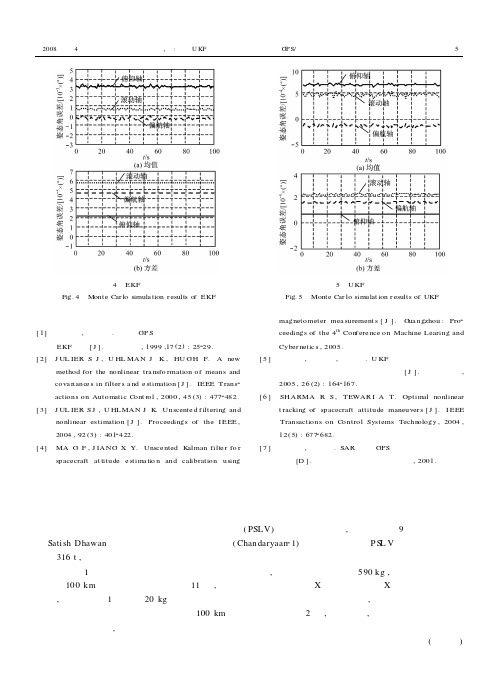
图4 EKF 仿真结果Fig.4 Monte Car lo simula tion r esults o fEKF图5 UKF 仿真结果Fig.5 Monte Car lo simulat ion r esults of UKF 参考文献[1] 罗建军,袁建平.利用GP S 进行航天器姿态确定的EKF 方法[J ].航天控制,1999,17(2):25229.[2] J UL IER S J ,U HL MAN J K ,HU GH F.A newmethod for the nonlinear tra nsfo rmation of means and cova riance s in filter s a nd e stimation [J ].IEEE Trans 2actions on Automatic Cont rol ,2000,45(3):4772482.[3] J UL IER S J ,U HLMAN J K .Unscente d f iltering andnonlinear estimation [J ].Proceedings of the I EEE ,2004,92(3):4012422.[4] MA G F ,J IANG X Y.Unsce nted K alman filte r fo rspacecraft at titude e stima tio n and calibration usingmagnetometer mea surement s [J ].G ua ngzhou :Pro 2ceedings of the 4th Con f ere nce on Machine Learing and Cyber netic s ,2005.[5] 张红梅,邓正隆,高玉凯.U KF 在基于修正罗得里格参数的飞行器姿态确定中的应用[J ].宇航学报,2005,26(2):1642167.[6] SHARMA R S ,TEWAR I A T.Optimal nonlineart racking of spacecraft attitude maneuver s [J ].I EEE Transactions on Control Systems Techn ology ,2004,12(5):6772682.[7] 张贵明,黄顺吉.SAR 卫星GPS 轨道和姿态测量技术研究[D ].电子科技大学博士学位论文,2001.印度月球初航航天器即将发射印度太空研究组织的增强型极轨卫星运载火箭(PSLV)的装配已经开始,准备在今年9月从印度东海岸Sati sh Dhawan 航天中心发射印度的月球初航(Chandaryaan 21)任务。

SIAM REV SIAM REVIEWJ AM MATH SOC JOURNAL OF THE AMERICAN MATHEMATICAL SOCIETYANN MATH ANNALS OF MATHEMATICSB AM MATH SOC BULLETIN OF THE AMERICAN MATHEMATICAL SOCIETYJ R STAT SOC B JOURNAL OF THE ROYAL STATISTICAL SOCIETY SERIES B-STATIS J AM STAT ASSOC JOURNAL OF THE AMERICAN STATISTICAL ASSOCIATION STRUCT EQU MODELING STRUCTURAL EQUATION MODELING-A MULTIDISCIPLINARY JOURNAL MULTIVAR BEHAV RES MULTIVARIATE BEHAVIORAL RESEARCHINT J INFECT DIS DYNAMICS OF CONTINUOUS DISCRETE AND IMPULSIVE SYSTEMS-SE COMMUN PUR APPL MATH COMMUNICATIONS ON PURE AND APPLIED MATHEMATICSRISK ANAL RISK ANALYSISANN STAT ANNALS OF STATISTICSSIAM J SCI COMPUT SIAM JOURNAL ON SCIENTIFIC COMPUTINGMATH MOD METH APPL S MATHEMATICAL MODELS & METHODS IN APPLIED SCIENCESSIAM J MATRIX ANAL A SIAM JOURNAL ON MATRIX ANALYSIS AND APPLICATIONS MULTISCALE MODEL SIM MULTISCALE MODELING & SIMULATIONINVENT MATH INVENTIONES MATHEMATICAEJ R STAT SOC A STAT JOURNAL OF THE ROYAL STATISTICAL SOCIETY SERIES A-STATIS STAT SCI STATISTICAL SCIENCEJ EUR MATH SOC JOURNAL OF THE EUROPEAN MATHEMATICAL SOCIETYSIAM J APPL MATH SIAM JOURNAL ON APPLIED MATHEMATICSDUKE MATH J DUKE MATHEMATICAL JOURNALPUBL MATH-PARIS PUBLICATIONS MATHEMATIQUES DE L IHESSIAM J NUMER ANAL SIAM JOURNAL ON NUMERICAL ANALYSISACTA MATH-DJURSHOLM ACTA MATHEMATICAINVERSE PROBL INVERSE PROBLEMSSTAT COMPUT STATISTICS AND COMPUTINGANN PROBAB ANNALS OF PROBABILITYANN I H POINCARE-AN ANNALES DE L INSTITUT HENRI POINCARE-ANALYSE NON LINEAIR J SCI COMPUT JOURNAL OF SCIENTIFIC COMPUTINGGEOM TOPOL GEOMETRY & TOPOLOGYFOUND COMPUT MATH FOUNDATIONS OF COMPUTATIONAL MATHEMATICSSIAM J CONTROL OPTIM SIAM JOURNAL ON CONTROL AND OPTIMIZATIONAPPL COMPUT HARMON A APPLIED AND COMPUTATIONAL HARMONIC ANALYSISANN APPL PROBAB ANNALS OF APPLIED PROBABILITYSIAM J OPTIMIZ SIAM JOURNAL ON OPTIMIZATIONLECT NOTES MATH LECTURE NOTES IN MATHEMATICSNONLINEAR ANAL-REAL NONLINEAR ANALYSIS-REAL WORLD APPLICATIONSBOREAL ENVIRON RES ANNALES ACADEMIAE SCIENTIARUM FENNICAE-MATHEMATICA FUZZY SET SYST FUZZY SETS AND SYSTEMSPROBAB THEORY REL PROBABILITY THEORY AND RELATED FIELDSRANDOM STRUCT ALGOR RANDOM STRUCTURES & ALGORITHMSJ DIFFER EQUATIONS JOURNAL OF DIFFERENTIAL EQUATIONSJ MATH PURE APPL JOURNAL DE MATHEMATIQUES PURES ET APPLIQUEESIMA J NUMER ANAL IMA JOURNAL OF NUMERICAL ANALYSISMATH COMPUT MATHEMATICS OF COMPUTATIONADV MATH ADVANCES IN MATHEMATICSSIAM J MATH ANAL SIAM JOURNAL ON MATHEMATICAL ANALYSISCOMPUT COMPLEX COMPUTATIONAL COMPLEXITYJ ALGORITHM JOURNAL OF ALGORITHMSNUMER MATH NUMERISCHE MATHEMATIKGEOM FUNCT ANAL GEOMETRIC AND FUNCTIONAL ANALYSISMATH FINANC MATHEMATICAL FINANCECONSTR APPROX CONSTRUCTIVE APPROXIMATIONCOMMUN PART DIFF EQ COMMUNICATIONS IN PARTIAL DIFFERENTIAL EQUATIONS INTERFACE FREE BOUND INTERFACES AND FREE BOUNDARIESDISCRETE CONT DYN S DISCRETE AND CONTINUOUS DYNAMICAL SYSTEMSMEM AM MATH SOC MEMOIRS OF THE AMERICAN MATHEMATICAL SOCIETYB SOC MATH FR BULLETIN DE LA SOCIETE MATHEMATIQUE DE FRANCEJ R STAT SOC C-APPL JOURNAL OF THE ROYAL STATISTICAL SOCIETY SERIES C-APPLIE ANN SCI ECOLE NORM S ANNALES SCIENTIFIQUES DE L ECOLE NORMALE SUPERIEUREJ DIFFER EQU APPL JOURNAL OF DIFFERENCE EQUATIONS AND APPLICATIONSSTUD APPL MATH STUDIES IN APPLIED MATHEMATICSINDIANA U MATH J INDIANA UNIVERSITY MATHEMATICS JOURNALCOMPLEXITY COMPLEXITYBERNOULLI BERNOULLIJ BUS ECON STAT JOURNAL OF BUSINESS & ECONOMIC STATISTICSJ COMPUT GRAPH STAT JOURNAL OF COMPUTATIONAL AND GRAPHICAL STATISTICSCALC VAR PARTIAL DIF CALCULUS OF VARIATIONS AND PARTIAL DIFFERENTIAL EQUATION AM STAT AMERICAN STATISTICIANDISCRETE CONT DYN-B DISCRETE AND CONTINUOUS DYNAMICAL SYSTEMS-SERIES BJ ALGEBRAIC GEOM JOURNAL OF ALGEBRAIC GEOMETRYAM J MATH AMERICAN JOURNAL OF MATHEMATICSCOMPUT STAT DATA AN COMPUTATIONAL STATISTICS & DATA ANALYSISSCAND J STAT SCANDINAVIAN JOURNAL OF STATISTICSP LOND MATH SOC PROCEEDINGS OF THE LONDON MATHEMATICAL SOCIETYMATH ANN MATHEMATISCHE ANNALENSTAT MODEL STATISTICAL MODELLINGDISCRETE MATH THEOR DISCRETE MATHEMATICS AND THEORETICAL COMPUTER SCIENCE ADV COMPUT MATH ADVANCES IN COMPUTATIONAL MATHEMATICSJ FUNCT ANAL JOURNAL OF FUNCTIONAL ANALYSISINT J BIFURCAT CHAOS INTERNATIONAL JOURNAL OF BIFURCATION AND CHAOSJ REINE ANGEW MATH JOURNAL FUR DIE REINE UND ANGEWANDTE MATHEMATIKNUMER LINEAR ALGEBR NUMERICAL LINEAR ALGEBRA WITH APPLICATIONSCOMMUN PUR APPL ANAL COMMUNICATIONS ON PURE AND APPLIED ANALYSIS ALGORITHMICA ALGORITHMICABIT BITAPPL NUMER MATH APPLIED NUMERICAL MATHEMATICSTOPOLOGY TOPOLOGYT AM MATH SOC TRANSACTIONS OF THE AMERICAN MATHEMATICAL SOCIETYINT STAT REV INTERNATIONAL STATISTICAL REVIEWINT MATH RES NOTICES INTERNATIONAL MATHEMATICS RESEARCH NOTICESAPPL MATH COMPUT APPLIED MATHEMATICS AND COMPUTATIONJ GEOM ANAL JOURNAL OF GEOMETRIC ANALYSISEUR J APPL MATH EUROPEAN JOURNAL OF APPLIED MATHEMATICSSTAT SINICA STATISTICA SINICASTOCH PROC APPL STOCHASTIC PROCESSES AND THEIR APPLICATIONSCOMPUT OPTIM APPL COMPUTATIONAL OPTIMIZATION AND APPLICATIONSJ COMB THEORY B JOURNAL OF COMBINATORIAL THEORY SERIES BADV APPL PROBAB ADVANCES IN APPLIED PROBABILITYCOMMENT MATH HELV COMMENTARII MATHEMATICI HELVETICICOMBINATORICA COMBINATORICAADV NONLINEAR STUD ADVANCED NONLINEAR STUDIESTHEOR COMPUT SYST THEORY OF COMPUTING SYSTEMSADV APPL MATH ADVANCES IN APPLIED MATHEMATICSJ MULTIVARIATE ANAL JOURNAL OF MULTIVARIATE ANALYSISJ FOURIER ANAL APPL JOURNAL OF FOURIER ANALYSIS AND APPLICATIONSJ COMPUT APPL MATH JOURNAL OF COMPUTATIONAL AND APPLIED MATHEMATICSJ MATH ANAL APPL JOURNAL OF MATHEMATICAL ANALYSIS AND APPLICATIONSJ COMB DES JOURNAL OF COMBINATORIAL DESIGNSANN I H POINCARE-PR ANNALES DE L INSTITUT HENRI POINCARE-PROBABILITES ET STA J DIFFER GEOM JOURNAL OF DIFFERENTIAL GEOMETRYELECTRON T NUMER ANA ELECTRONIC TRANSACTIONS ON NUMERICAL ANALYSIS TRANSFORM GROUPS TRANSFORMATION GROUPSCOMMUN ANAL GEOM COMMUNICATIONS IN ANALYSIS AND GEOMETRYIMA J APPL MATH IMA JOURNAL OF APPLIED MATHEMATICSEUR J COMBIN EUROPEAN JOURNAL OF COMBINATORICSSET-VALUED ANAL SET-VALUED ANALYSISANN I FOURIER ANNALES DE L INSTITUT FOURIERCAN J STAT CANADIAN JOURNAL OF STATISTICS-REVUE CANADIENNE DE STATI ERGOD THEOR DYN SYST ERGODIC THEORY AND DYNAMICAL SYSTEMSFORUM MATH FORUM MATHEMATICUMP ROY SOC EDINB A PROCEEDINGS OF THE ROYAL SOCIETY OF EDINBURGH SECTION A-J EVOL EQU JOURNAL OF EVOLUTION EQUATIONSJ COMB THEORY A JOURNAL OF COMBINATORIAL THEORY SERIES ANONLINEAR ANAL-THEOR NONLINEAR ANALYSIS-THEORY METHODS & APPLICATIONSESAIM-MATH MODEL NUM ESAIM-MATHEMATICAL MODELLING AND NUMERICAL ANALYSIS-MODE ELECTRON J PROBAB ELECTRONIC JOURNAL OF PROBABILITYCOMPOS MATH COMPOSITIO MATHEMATICAREV MAT IBEROAM REVISTA MATEMATICA IBEROAMERICANACOMMUN CONTEMP MATH COMMUNICATIONS IN CONTEMPORARY MATHEMATICSNUMER METH PART D E NUMERICAL METHODS FOR PARTIAL DIFFERENTIAL EQUATIONS COMB PROBAB COMPUT COMBINATORICS PROBABILITY & COMPUTINGELECTRON RES ANNOUNC ELECTRONIC RESEARCH ANNOUNCEMENTS OF THE AMERICAN MATHEM J SYMBOLIC LOGIC JOURNAL OF SYMBOLIC LOGICMATH RES LETT MATHEMATICAL RESEARCH LETTERSASTERISQUE ASTERISQUEPOTENTIAL ANAL POTENTIAL ANALYSISZ ANGEW MATH PHYS ZEITSCHRIFT FUR ANGEWANDTE MATHEMATIK UND PHYSIK NODEA-NONLINEAR DIFF NODEA-NONLINEAR DIFFERENTIAL EQUATIONS AND APPLICATIONS COMP GEOM-THEOR APPL COMPUTATIONAL GEOMETRY-THEORY AND APPLICATIONSB SCI MATH BULLETIN DES SCIENCES MATHEMATIQUESJ TIME SER ANAL JOURNAL OF TIME SERIES ANALYSISDESIGN CODE CRYPTOGR DESIGNS CODES AND CRYPTOGRAPHYINFIN DIMENS ANAL QU INFINITE DIMENSIONAL ANALYSIS QUANTUM PROBABILITY AND RE J OPTIMIZ THEORY APP JOURNAL OF OPTIMIZATION THEORY AND APPLICATIONSMATH LOGIC QUART MATHEMATICAL LOGIC QUARTERLYJ LOND MATH SOC JOURNAL OF THE LONDON MATHEMATICAL SOCIETY-SECOND SERIES J COMB OPTIM JOURNAL OF COMBINATORIAL OPTIMIZATIONJ ORTHOP SCI FINANCE AND STOCHASTICSPSYCHOMETRIKA PSYCHOMETRIKAJ CLASSIF JOURNAL OF CLASSIFICATIONMATH PHYS ANAL GEOM MATHEMATICAL PHYSICS ANALYSIS AND GEOMETRYJ MATH SOC JPN JOURNAL OF THE MATHEMATICAL SOCIETY OF JAPANISR J MATH ISRAEL JOURNAL OF MATHEMATICSLINEAR ALGEBRA APPL LINEAR ALGEBRA AND ITS APPLICATIONSAPPL MATH MODEL APPLIED MATHEMATICAL MODELLINGANN PURE APPL LOGIC ANNALS OF PURE AND APPLIED LOGICTEST TESTDISCRETE APPL MATH DISCRETE APPLIED MATHEMATICSADV GEOM ADVANCES IN GEOMETRYQ J MATH QUARTERLY JOURNAL OF MATHEMATICSANN SCUOLA NORM-SCI ANNALI DELLA SCUOLA NORMALE SUPERIORE DI PISA-CLASSE DI MATH Z MATHEMATISCHE ZEITSCHRIFTJ ALGEBRA JOURNAL OF ALGEBRAJ CONVEX ANAL JOURNAL OF CONVEX ANALYSISB LOND MATH SOC BULLETIN OF THE LONDON MATHEMATICAL SOCIETYFINITE FIELDS TH APP FINITE FIELDS AND THEIR APPLICATIONSEXP MATH EXPERIMENTAL MATHEMATICSSTAT NEERL STATISTICA NEERLANDICAMETRIKA METRIKAARCH MATH LOGIC ARCHIVE FOR MATHEMATICAL LOGICAPPL MATH LETT APPLIED MATHEMATICS LETTERSIZV MATH+IZVESTIYA MATHEMATICSMATH PROC CAMBRIDGE MATHEMATICAL PROCEEDINGS OF THE CAMBRIDGE PHILOSOPHICAL ZAMM-Z ANGEW MATH ME ZAMM-Zeitschrift fur Angewandte Mathematik und Mechanik MATH COMPUT SIMULAT MATHEMATICS AND COMPUTERS IN SIMULATIONINT J MATH INTERNATIONAL JOURNAL OF MATHEMATICSJ OPERAT THEOR JOURNAL OF OPERATOR THEORYB SYMB LOG BULLETIN OF SYMBOLIC LOGICSIAM J DISCRETE MATH SIAM JOURNAL ON DISCRETE MATHEMATICSSTUD MATH STUDIA MATHEMATICAP AM MATH SOC PROCEEDINGS OF THE AMERICAN MATHEMATICAL SOCIETYJ LIE THEORY JOURNAL OF LIE THEORYQ APPL MATH QUARTERLY OF APPLIED MATHEMATICSJ APPL PROBAB JOURNAL OF APPLIED PROBABILITYJ APPROX THEORY JOURNAL OF APPROXIMATION THEORYJ HYPERBOL DIFFER EQ Journal of Hyperbolic Differential Equations OPTIMIZATION OPTIMIZATIONDISCRETE DYN NAT SOC DISCRETE DYNAMICS IN NATURE AND SOCIETYJ STAT PLAN INFER JOURNAL OF STATISTICAL PLANNING AND INFERENCEADV COMPLEX SYST ADVANCES IN COMPLEX SYSTEMSOSAKA J MATH OSAKA JOURNAL OF MATHEMATICSINTEGR EQUAT OPER TH INTEGRAL EQUATIONS AND OPERATOR THEORYJ MATH SOCIOL JOURNAL OF MATHEMATICAL SOCIOLOGYJ APPL STAT JOURNAL OF APPLIED STATISTICSJ NUMBER THEORY JOURNAL OF NUMBER THEORYDISCRETE COMPUT GEOM DISCRETE & COMPUTATIONAL GEOMETRYJ KNOT THEOR RAMIF JOURNAL OF KNOT THEORY AND ITS RAMIFICATIONSMATH METHOD APPL SCI MATHEMATICAL METHODS IN THE APPLIED SCIENCESJ PURE APPL ALGEBRA JOURNAL OF PURE AND APPLIED ALGEBRACHINESE ANN MATH B CHINESE ANNALS OF MATHEMATICS SERIES BAPPL CATEGOR STRUCT APPLIED CATEGORICAL STRUCTURESNUMER ALGORITHMS NUMERICAL ALGORITHMSASYMPTOTIC ANAL ASYMPTOTIC ANALYSISCAN J MATH CANADIAN JOURNAL OF MATHEMATICS-JOURNAL CANADIEN DE MATH NAGOYA MATH J NAGOYA MATHEMATICAL JOURNALSTATISTICS STATISTICSK-THEORY K-THEORYINT J COMPUT GEOM AP INTERNATIONAL JOURNAL OF COMPUTATIONAL GEOMETRY & APPLIC LIFETIME DATA ANAL LIFETIME DATA ANALYSISAPPL STOCH MODEL BUS APPLIED STOCHASTIC MODELS IN BUSINESS AND INDUSTRYCR MATH COMPTES RENDUS MATHEMATIQUEMICH MATH J MICHIGAN MATHEMATICAL JOURNALACTA MATH SIN ACTA MATHEMATICA SINICA-ENGLISH SERIESMONATSH MATH MONATSHEFTE FUR MATHEMATIKANN GLOB ANAL GEOM ANNALS OF GLOBAL ANALYSIS AND GEOMETRYMATH COMPUT MODEL MATHEMATICAL AND COMPUTER MODELLINGJ GROUP THEORY JOURNAL OF GROUP THEORYINT J COMPUT MATH INTERNATIONAL JOURNAL OF COMPUTER MATHEMATICSACTA APPL MATH ACTA APPLICANDAE MATHEMATICAEPUBL MAT PUBLICACIONS MATEMATIQUESINT J GAME THEORY INTERNATIONAL JOURNAL OF GAME THEORYPAC J MATH PACIFIC JOURNAL OF MATHEMATICSGEOMETRIAE DEDICATA GEOMETRIAE DEDICATAPUBL RES I MATH SCI PUBLICATIONS OF THE RESEARCH INSTITUTE FOR MATHEMATICAL DIFFER GEOM APPL DIFFERENTIAL GEOMETRY AND ITS APPLICATIONSJ ANAL MATH JOURNAL D ANALYSE MATHEMATIQUENUMER FUNC ANAL OPT NUMERICAL FUNCTIONAL ANALYSIS AND OPTIMIZATIONJ GRAPH THEOR JOURNAL OF GRAPH THEORYDYNAM SYST APPL DYNAMIC SYSTEMS AND APPLICATIONSFUND MATH FUNDAMENTA MATHEMATICAEINDAGAT MATH NEW SER INDAGATIONES MATHEMATICAE-NEW SERIESSTOCH MODELS STOCHASTIC MODELSARK MAT ARKIV FOR MATEMATIKJ ALGEBR COMB JOURNAL OF ALGEBRAIC COMBINATORICSTOPOL APPL TOPOLOGY AND ITS APPLICATIONSJ COMPUT MATH JOURNAL OF COMPUTATIONAL MATHEMATICSMATH METHOD OPER RES MATHEMATICAL METHODS OF OPERATIONS RESEARCHACTA MATH HUNG ACTA MATHEMATICA HUNGARICAJ THEOR PROBAB JOURNAL OF THEORETICAL PROBABILITYMATH NACHR MATHEMATISCHE NACHRICHTENMATH SCAND MATHEMATICA SCANDINAVICAMANUSCRIPTA MATH MANUSCRIPTA MATHEMATICAILLINOIS J MATH ILLINOIS JOURNAL OF MATHEMATICSJPN J IND APPL MATH JAPAN JOURNAL OF INDUSTRIAL AND APPLIED MATHEMATICS SEMIGROUP FORUM SEMIGROUP FORUMP EDINBURGH MATH SOC PROCEEDINGS OF THE EDINBURGH MATHEMATICAL SOCIETYZ ANAL ANWEND ZEITSCHRIFT FUR ANALYSIS UND IHRE ANWENDUNGENINT J ALGEBR COMPUT INTERNATIONAL JOURNAL OF ALGEBRA AND COMPUTATION TAIWAN J MATH TAIWANESE JOURNAL OF MATHEMATICSANN I STAT MATH ANNALS OF THE INSTITUTE OF STATISTICAL MATHEMATICS HOUSTON J MATH HOUSTON JOURNAL OF MATHEMATICSDISCRETE MATH DISCRETE MATHEMATICSAUST NZ J STAT AUSTRALIAN & NEW ZEALAND JOURNAL OF STATISTICSACTA ARITH ACTA ARITHMETICAARCH MATH ARCHIV DER MATHEMATIKMATH INEQUAL APPL MATHEMATICAL INEQUALITIES & APPLICATIONSSTOCH ANAL APPL STOCHASTIC ANALYSIS AND APPLICATIONSMATH INTELL MATHEMATICAL INTELLIGENCEREXPO MATH EXPOSITIONES MATHEMATICAEGLASGOW MATH J GLASGOW MATHEMATICAL JOURNALJ KOREAN MATH SOC JOURNAL OF THE KOREAN MATHEMATICAL SOCIETYELECTRON J LINEAR AL Electronic Journal of Linear AlgebraRAMANUJAN J RAMANUJAN JOURNALMATH SOC SCI MATHEMATICAL SOCIAL SCIENCESLINEAR MULTILINEAR A LINEAR & MULTILINEAR ALGEBRARUSS MATH SURV+RUSSIAN MATHEMATICAL SURVEYSTHEOR PROBAB APPL+THEORY OF PROBABILITY AND ITS APPLICATIONSTOHOKU MATH J TOHOKU MATHEMATICAL JOURNALSB MATH+SBORNIK MATHEMATICSMETHODOL COMPUT APPL METHODOLOGY AND COMPUTING IN APPLIED PROBABILITYSTAT PROBABIL LETT STATISTICS & PROBABILITY LETTERSANZIAM J ANZIAM JOURNALRUSS J NUMER ANAL M RUSSIAN JOURNAL OF NUMERICAL ANALYSIS AND MATHEMATICAL M ALGEBR REPRESENT TH ALGEBRAS AND REPRESENTATION THEORYPUBL MATH-DEBRECEN PUBLICATIONES MATHEMATICAE-DEBRECENSTAT PAP STATISTICAL PAPERSJ NONPARAMETR STAT JOURNAL OF NONPARAMETRIC STATISTICSJ MATH KYOTO U JOURNAL OF MATHEMATICS OF KYOTO UNIVERSITYCOMMUN ALGEBRA COMMUNICATIONS IN ALGEBRAUTILITAS MATHEMATICA UTILITAS MATHEMATICAJ AUST MATH SOC JOURNAL OF THE AUSTRALIAN MATHEMATICAL SOCIETYB AUST MATH SOC BULLETIN OF THE AUSTRALIAN MATHEMATICAL SOCIETYP JPN ACAD A-MATH PROCEEDINGS OF THE JAPAN ACADEMY SERIES A-MATHEMATICAL S INTEGR TRANSF SPEC F INTEGRAL TRANSFORMS AND SPECIAL FUNCTIONSCAN MATH BULL CANADIAN MATHEMATICAL BULLETIN-BULLETIN CANADIEN DE MATH FUNCT ANAL APPL+FUNCTIONAL ANALYSIS AND ITS APPLICATIONSB BRAZ MATH SOC BULLETIN BRAZILIAN MATHEMATICAL SOCIETYAM MATH MON AMERICAN MATHEMATICAL MONTHLYCOMMUN STAT-THEOR M COMMUNICATIONS IN STATISTICS-THEORY AND METHODS ALGEBRA UNIV ALGEBRA UNIVERSALISLOGIC J IGPL LOGIC JOURNAL OF THE IGPLMATH COMP MODEL DYN MATHEMATICAL AND COMPUTER MODELLING OF DYNAMICAL SYSTEMS DIFF EQUAT+DIFFERENTIAL EQUATIONSJ STAT COMPUT SIM JOURNAL OF STATISTICAL COMPUTATION AND SIMULATION COMPUTATION STAT COMPUTATIONAL STATISTICSSIBERIAN MATH J+SIBERIAN MATHEMATICAL JOURNALCZECH MATH J CZECHOSLOVAK MATHEMATICAL JOURNALDYNAM CONT DIS SER B DYNAMICS OF CONTINUOUS DISCRETE AND IMPULSIVE SYSTEMS-SE APPL MATH MECH-ENGL PROCEEDINGS OF THE INDIAN ACADEMY OF SCIENCES-MATHEMATIC REND SEMIN MAT U PAD RENDICONTI DEL SEMINARIO MATEMATICO DELLA UNIVERSITA DI ROCKY MT J MATH ROCKY MOUNTAIN JOURNAL OF MATHEMATICSALGEBR COLLOQ ALGEBRA COLLOQUIUMSTUD SCI MATH HUNG STUDIA SCIENTIARUM MATHEMATICARUM HUNGARICAGRAPH COMBINATOR GRAPHS AND COMBINATORICSCOMMUN STAT-SIMUL C COMMUNICATIONS IN STATISTICS-SIMULATION AND COMPUTATION MATH NOTES+MATHEMATICAL NOTESACTA MATH SCI ACTA MATHEMATICA SCIENTIAB BELG MATH SOC-SIM BULLETIN OF THE BELGIAN MATHEMATICAL SOCIETY-SIMON STEVI BOL SOC MAT MEX BOLETIN DE LA SOCIEDAD MATEMATICA MEXICANAORDER ORDER-A JOURNAL ON THE THEORY OF ORDERED SETS AND ITS AP POSITIVITY POSITIVITYCALCOLO CALCOLOARS COMBINATORIA ARS COMBINATORIAHIST MATH HISTORIA MATHEMATICAABH MATH SEM HAMBURG ABHANDLUNGEN AUS DEM MATHEMATISCHEN SEMINAR DER UNIVERSI INDIAN J PURE AP MAT INDIAN JOURNAL OF PURE & APPLIED MATHEMATICS FIBONACCI QUART FIBONACCI QUARTERLYDOKL MATH DOKLADY MATHEMATICS0036-1445数学 2.6677.2 6.118 5.3326672922245921782519.66667 0894-0347数学 2.552 2.3 2.581 2.4853331457123011041263.66667 0003-486X数学 2.4262 1.845 2.0933336285529654555678.66667 0273-0979数学 2.385 1.8 2.962 2.3823332304194919862079.66667 1369-7412数学 2.3152 2.691 2.3223337168629556426368.33333 0162-1459数学 2.171 1.7 1.978 1.95314510131941272513476.3333 1070-5511数学 2.143 1.2 1.919 1.7693332549209317812141 0027-3171数学 2.095 1.20.952 1.4033331394124610551231.66667 1201-9712数学 2.0620.20.0860.7943335114920193.333333 0010-3640数学 2.031 1.8 1.694 1.8553334407390038584055 0272-4332数学 1.938 1.5 1.321 1.5896672521204419772180.66667 0090-5364数学 1.902 1.7 1.625 1.7347253631061186560.33333 1064-8275数学 1.824 1.5 1.231 1.5213334360367731623733 0218-2025数学 1.805 1.2 1.31 1.454333894768674778.666667 0895-4798数学 1.798 1.10.727 1.2243331658149711341429.66667 1540-3459数学 1.723 1.7 1.135 1.52966727814955160.666667 0020-9910数学 1.659 1.7 1.926 1.7456675025443846424701.66667 0964-1998数学 1.547 1.10.796 1.1393331296119310991196 0883-4237数学 1.531 1.8 1.423 1.6011599139712301408.66667 1435-9855数学 1.486 1.40.95 1.28333318311888129.666667 0036-1399数学 1.425 1.1 1.189 1.2446673682339732123430.33333 0012-7094数学 1.409 1.3 1.118 1.2773147278427622897.66667 0073-8301数学 1.353 1.2 1.529 1.354667760690809753 0036-1429数学 1.335 1.4 1.106 1.2776675308439936234443.33333 0001-5962数学 1.333 1.8 2.2 1.7703332103193419451994 0266-5611数学 1.319 1.5 1.344 1.4013332264208417242024 0960-3174数学 1.3050.80.7610.938667675530484563 0091-1798数学 1.301 1.1 1.189 1.2073332521222424382394.33333 0294-1449数学 1.29210.753 1.024873795718795.333333 0885-7474数学 1.281 1.70.978672543405 1364-0380数学 1.274 1.30.849667386236207.333333 1615-3375数学 1.2690.9 1.5 1.216333127826491 0363-0129数学 1.263 1.2 1.048 1.1553548306026333080.33333 1063-5203数学 1.226 1.4 1.456 1.354741603581641.666667 1050-5164数学 1.211 1.4 1.37 1.317108810709661041.33333 1052-6234数学 1.211 1.2 1.213 1.2206671816166413091596.33333 0075-8434数学 1.2060.40273042434.66667 1468-1218数学 1.1940.70.4770.77666722311777139 1239-6095数学 1.1880.50.5560.736667327412373370.666667 0165-0114数学 1.18110.7340.9846676477474544055209 0178-8051数学 1.180.9 1.164 1.081330122613771311 1042-9832数学 1.16710.966 1.052333779633614675.333333 0022-0396数学 1.1660.90.8770.9933334386360433583782.666670021-7824数学 1.161 1.20.926 1.09412059929601052.33333 0272-4979数学 1.159 1.30.75 1.055667658583458566.333333 0025-5718数学 1.1550.90.9130.9736674119353834383698.33333 0001-8708数学 1.1431 1.067 1.0672589221821942333.66667 0036-1410数学 1.134 1.10.966 1.0532379209919722150 1016-3328数学 1.12520.615 1.246667382391354375.666667 0196-6774数学 1.119 1.10.849 1.0353331219125311581210 0029-599X数学 1.116 1.2 1.011 1.1163333339313027023057 1016-443X数学 1.11510.8890.99812663572682.333333 0960-1627数学 1.102 1.3 1.9 1.449639672606639 0176-4276数学 1.0940.90.5780.860333580542394505.333333 0360-5302数学 1.0940.70.6710.8286671797141413991536.66667 1463-9971数学 1.0911 1.205 1.106667164126104131.333333 1078-0947数学 1.08710.994 1.035333707554468576.333333 0065-9266数学 1.077 1.3 1.193 1.1951334124212391271.66667 0037-9484数学 1.0730.50.50.702667799743789777 0035-9254数学 1.0720.60.4630.725333864798850837.333333 0012-9593数学 1.0711 1.186 1.0856671054106210981071.33333 1023-6198数学 1.0470.60.6710.777667552316256374.666667 0022-2526数学 1.0310.70.5360.756825716654731.666667 0022-2518数学 1.0290.80.7840.8606671784155515281622.33333 1076-2787数学 1.018 1.10.689667275266180.333333 1350-7265数学 1.0110.70.9640.890333491399442444 0735-0015数学11 1.208 1.0606671816160113841600.33333 1061-8600数学10.8 1.0810.9486671266113911181174.33333 0944-2669数学0.9920.90.7860.879667573481404486 0003-1305数学0.9760.90.7830.8771750146513801531.66667 1531-3492数学0.9721 1.31 1.11290236155227 1056-3911数学0.9670.70.7760.801333364336333344.333333 0002-9327数学0.93310.9380.9496672618249325392550 0167-9473数学0.9280.7 1.0220.89433312849128831026.33333 0303-6898数学0.9030.80.8490.8581104914911976.333333 0024-6115数学0.9020.80.8720.8636672277214320832167.66667 0025-5831数学0.9020.80.790.844124360237003808.66667 1471-082X数学0.90.60.4983331569985 1365-8050数学0.895 1.10.5930.849667106876385.3333333 1019-7168数学0.868 1.10.7630.924667710602488600 0022-1236数学0.8660.80.9620.8784066350435893719.66667 0218-1274数学0.8660.8 1.0190.912978270225322737.33333 0075-4102数学0.860.90.8850.8823332735260126642666.66667 1070-5325数学0.860.80.7270.792667560457334450.333333 1534-0392数学0.8570.40.6180.636162704492 0178-4617数学0.8510.9230.931225120111441190 0006-3835数学0.8410.50.5620.637333876820730808.666667 0168-9274数学0.8350.60.6390.687667128310379461088.66667 0040-9383数学0.8260.80.7270.7743331642150515121553 0002-9947数学0.820.80.8390.8286677527681164696935.666670306-7734数学0.820.80.6940.771333632528559573 1073-7928数学0.8170.70.9060.8153331036793631820 0096-3003数学0.8160.70.5670.6903333518221114192382.66667 1050-6926数学0.8140.271333302100.666667 0956-7925数学0.8080.50.6150.657399347295347 1017-0405数学0.8080.9 1.55 1.0946671068888814923.333333 0304-4149数学0.8020.90.9040.8612171194720452054.33333 0926-6003数学0.80.90.8150.833667508448320425.333333 0095-8956数学0.7920.70.6180.6896671308123612721272 0001-8678数学0.7890.70.7660.7626671198119112931227.33333 0010-2571数学0.7840.90.8160.8203331051931923968.333333 0209-9683数学0.7840.80.3880.671333977878862905.666667 1536-1365数学0.7780.40.3060.50592412753.3333333 1432-4350数学0.7690.80.5380.708333193182132169 0196-8858数学0.7640.80.7330.774333679563550597.333333 0047-259X数学0.7630.70.4080.639121010579681078.33333 1069-5869数学0.7610.90.7970.805667473363402412.666667 0377-0427数学0.7590.60.4860.6046672971260820382539 0022-247X数学0.7580.60.490.6097816608060046633.33333 1063-8539数学0.7570.50.6620.637333244216269243 0246-0203数学0.7470.60.8620.743411361367379.666667 0022-040X数学0.7440.70.8630.7612123189718951971.66667 1068-9613数学0.7380.60.5650.637218166110164.666667 1083-4362数学0.7350.50.5710.606667202136165167.666667 1019-8385数学0.7280.50.5950.61378278258304.666667 0272-4960数学0.7250.60.6270.640333431347351376.333333 0195-6698数学0.710.30.3030.444333784625574661 0927-6947数学0.7070.80.5530.686667279263204248.666667 0373-0956数学0.6980.50.480.5583331121930938996.333333 0319-5724数学0.6960.50.6090.604333502479447476 0143-3857数学0.6910.70.4840.635122011079871104.66667 0933-7741数学0.690.60.5870.630333299266234266.333333 0308-2105数学0.6840.50.4870.5673331135103010521072.33333 1424-3199数学0.6790.70.6840.700333129866894.3333333 0097-3165数学0.6770.60.4850.5793331249116210541155 0362-546X数学0.6770.50.4590.5516673561278227003014.33333 0764-583X数学0.6760.90.560.697667416357241338 1083-6489数学0.6760.22533318060 0010-437X数学0.6750.80.9060.7796671221113411961183.66667 0213-2230数学0.6720.90.5650.697333444367379396.666667 0219-1997数学0.6670.70.5610.645333193173120162 0749-159X数学0.6670.70.6310.657333578415401464.666667 0963-5483数学0.6670.50.4040.52326220231259 1079-6762数学0.6670.40.320.44933377455258 0022-4812数学0.6640.50.3310.4883331509136112271365.66667 1073-2780数学0.6640.60.7160.670667749634626669.666667 0303-1179数学0.6580.40.570.53966710108931075992.6666670926-2601数学0.6570.50.570.582667312285262286.333333 0044-2275数学0.6520.50.5460.551928854778853.333333 1021-9722数学0.6520.30.3960.434333150101103118 0925-7721数学0.640.60.7420.670333808779765784 0007-4497数学0.6370.40.3850.479387321322343.333333 0143-9782数学0.6370.60.410.553333897718685766.666667 0925-1022数学0.6370.70.690.662667546500495513.666667 0219-0257数学0.6340.80.5690.671667520508447491.666667 0022-3239数学0.6330.60.5930.6126672236219017662064 0942-5616数学0.6290.40.2630.426240154136176.666667 0024-6107数学0.6170.70.6630.6586672031190318051913 1382-6905数学0.6150.30.560.488667213170158180.333333 0949-2658数学0.614 1.4 1.471 1.171333782397353510.666667 0033-3123数学0.6080.70.7850.6883333283335229993211.33333 0176-4268数学0.60.80.2270.548333398356286346.666667 1385-0172数学0.5930.70.7670.6973535761 0025-5645数学0.590.40.3660.465686641674667 0021-2172数学0.5860.40.410.4813331565141014751483.33333 0024-3795数学0.5850.60.5010.5586673748357430663462.66667 0307-904X数学0.5830.40.6170.544333859638610702.333333 0168-0072数学0.5820.50.5090.522333725600562629 1133-0686数学0.581 1.20.8810.875174163135157.333333 0166-218X数学0.5770.60.5570.5732036183216661844.66667 1615-715X数学0.5770.40.2820.43533395813971.6666667 0033-5606数学0.5740.90.4080.616667824713694743.666667 0391-173X数学0.5710.190333864288 0025-5874数学0.570.70.5460.5943332814244424322563.33333 0021-8693数学0.5680.50.5540.5274303387539394039 0944-6532数学0.5670.40.4250.456333187166142165 0024-6093数学0.5560.50.4040.479968851797872 1071-5797数学0.5560.30.5420.478667147100108118.333333 1058-6458数学0.5540.50.3560.466359300267308.666667 0039-0402数学0.5520.60.2930.489333214209173198.666667 0026-1335数学0.5510.50.390.464261222216233 1432-0665数学0.5480.50.2950.444333303250151234.666667 0893-9659数学0.5460.30.4140.4351177820762919.666667 1064-5632数学0.5450.60.398249265171.333333 0305-0041数学0.5360.50.4380.4981138106810721092.66667 0044-2267数学0.5340.40.29511411033724.666667 0378-4754数学0.5340.60.5120.533333840683643722 0129-167X数学0.5310.50.3230.440333412405347388 0379-4024数学0.5270.30.490.446667507455474478.666667 1079-8986数学0.5250.40.2780.404333169129118138.666667 0895-4801数学0.5180.90.6360.679667875852676801 0039-3223数学0.5150.50.5270.5266671310110712051207.33333 0002-9939数学0.5130.40.5080.4833335758505851785331.33333 0949-5932数学0.5070.30.280.36866713692811030033-569X数学0.5060.30.8520.5611376129813091327.66667 0021-9002数学0.5040.60.6350.5733331684159917491677.33333 0021-9045数学0.50.50.360.4436671028949736904.333333 0219-8916数学0.50.30.274333331114.6666667 0233-1934数学0.50.30.330.385377349301342.333333 1026-0226数学0.50.10.4810.37233367675964.3333333 0378-3758数学0.4970.50.4460.4746671521129212181343.66667 0219-5259数学0.4910.60.368667166192119.333333 0030-6126数学0.4850.40.2140.351667523428456469 0378-620X数学0.4810.50.5110.494681589590620 0022-250X数学0.480.60.1670.418667296247254265.666667 0266-4763数学0.480.30.6650.483667642486467531.666667 0022-314X数学0.4790.40.3880.407984803857881.333333 0179-5376数学0.4770.70.620.610667907944898916.333333 0218-2165数学0.4750.30.3080.368667427327246333.333333 0170-4214数学0.4730.50.4680.489730693677700 0022-4049数学0.470.60.4460.4891560150614181494.66667 0252-9599数学0.470.30.4310.406235234210226.333333 0927-2852数学0.4680.20.2920.3326671349193106 1017-1398数学0.4660.50.2640.395333470491326429 0921-7134数学0.4650.40.4250.438667389361354368 0008-414X数学0.4640.40.4460.4416671461148414061450.33333 0027-7630数学0.4640.30.2570.353333490460500483.333333 0233-1888数学0.4610.50.3230.425667368343368359.666667 0920-3036数学0.4580.50.4560.462667411350373378 0218-1959数学0.4490.40.4630.449242225190219 1380-7870数学0.4460.30.5330.430333230186173196.333333 1524-1904数学0.4430.30.2310.32214895101114.666667 1631-073X数学0.4430.50.2840.398667740566236514 0026-2285数学0.440.50.3870.428659590592613.666667 1439-8516数学0.440.30.4270.391667598406406470 0026-9255数学0.4390.40.3480.411333458402435431.666667 0232-704X数学0.4340.50.370.439333249202184211.666667 0895-7177数学0.4320.40.4790.4443331624134812151395.66667 1433-5883数学0.4290.50.4710.457333140107119122 0020-7160数学0.4280.30.2160.299333480405423436 0167-8019数学0.4250.50.3540.411667576473450499.666667 0214-1493数学0.4220.70.2410.440667130129111123.333333 0020-7276数学0.4110.20.2440.274667517519501512.333333 0030-8730数学0.4110.40.4650.4273332426222922282294.33333 0046-5755数学0.4080.30.4330.390333740608647665 0034-5318数学0.4070.40.2550.354544526486518.666667 0926-2245数学0.4070.40.4180.405333253195197215 0021-7670数学0.4050.50.6340.515727657633672.333333 0163-0563数学0.4050.30.3660.362385354284341 0364-9024数学0.4030.30.460.394865872844860.333333 1056-2176数学0.4030.20.2560.27833314190126119。

阈值期刊数期刊数3.4585225序号12345678910111213141516171819 2021 222324 25 26 2728 2930 31 32BIOTECCUBIOTECHNOLOGYAnnualBiomolecular EngineePROGRESSCHARACTERIZATION OF MACM CCHEMINTERNATIOPROCJOU377分区ADVANNUALRESEARCHNANaNATUEnergy EducPROGRESMATERIALSR-REPORTSPROGCOMBUSTION SCIENANNUALENGINEERINGPROGRETRENDADVANCEDNanomedicand MedicinePROGRE111111111111111111111111111111111062-7995PROG PHOTOVOLTAICS0018-9219P IEEE0021-9517J CATAL0950-6608INT MATER REV1549-9634NANOMED-NANOTECHNOL1947-5438ANNU REV CHEM BIOMOL1613-6810SMALL0960-8974PROG CRYST GROWTH CH1473-0197LAB CHIP0360-0300ACM COMPUT SURV1558-3724POLYM REV0897-4756CHEM MATER1369-7021MATER TODAY0142-9612BIOMATERIALS1531-7331ANNU REV MATER RES1936-0851ACS NANO0079-6816PROG SURF SCI0958-1669CURR OPIN BIOTECH0167-7799TRENDS BIOTECHNOL1616-301X ADV FUNCT MATER0734-9750BIOTECHNOL ADV0935-9648ADV MATER0927-796X MAT SCI ENG R1748-0132NANO TODAY0360-1285PROG ENERG COMBUST1530-6984NANO LETT1523-9829ANNU REV BIOMED ENG1748-3387NAT NANOTECHNOL1087-0156NAT BIOTECHNOL1301-8361ENERGY EDUC SCI TECH0079-6425PROG MATER SCI3区期刊数1区2区阈值阈值ISSN刊名简称1476-1122NAT MATER1.931 1.1123334 35 36 37 38 39 40 41 42 43 44 45 46 4748 49 50 51 5253 54 55 56 57 58 59 60 61 62 63 64BIORESADVANCEELCOMMUNICATIONSMOLECURESEARCHIEEE TRANELECTRONICSMACRCOMMUNICATIONSSOLAR ESOLAR CELLSJOURNACRITICAL RAND NUTRITIONCURRENTMATERIALS SCIENCINTERNCOMPUTER VISIONIEEEEVOLUTIONARY COMPUSIAM JoPROELECTRONICSJOURNAL OMETARENEWABLREVIEWSCRBIOTECHNOLOGYINTERNPLASTICITYBiotIEEE CoTutorialsIEEE SIGNAIEEE TRAANALYSIS AND MACHINTELLIGENCEMNBIOSENS111111111111111111111111111111111089-778X IEEE T EVOLUT COMPUT0278-0046IEEE T IND ELECTRON1022-1336MACROMOL RAPID COMM0927-0248SOL ENERG MAT SOL C0920-5691INT J COMPUT VISION0378-7753J POWER SOURCES1040-8398CRIT REV FOOD SCI1359-0286CURR OPIN SOLID ST M1388-2481ELECTROCHEM COMMUN1613-4125MOL NUTR FOOD RES1754-6834BIOTECHNOL BIOFUELS0276-7783MIS QUART1936-4954SIAM J IMAGING SCI0065-2156ADV APPL MECH1744-683X SOFT MATTER1742-7061ACTA BIOMATER0960-8524BIORESOURCE TECHNOL0024-9297MACROMOLECULES0749-6419INT J PLASTICITY1364-0321RENEW SUST ENERG REV0738-8551CRIT REV BIOTECHNOL2040-3364NANOSCALE0162-8828IEEE T PATTERN ANAL1553-877X IEEE COMMUN SURV TUT1053-5888IEEE SIGNAL PROC MAG0008-6223CARBON0959-9428J MATER CHEM1096-7176METAB ENG0883-7694MRS BULL1884-4049NPG ASIA MATER0956-5663BIOSENS BIOELECTRON0079-6727PROG QUANT ELECTRON65 6667 68 69 70 71 7273 74 75 7677 7879 8081 82 83 84 8586 87 8889 90 91 92 93 949596FJournMicrofINTERNNONLINEAR SCIENCESNUMERICAL SIMULATFOSENSOCHEMICALAPPLIED SIEEE JOURIN QUANTUM ELECTROIEEE TRSYSTEMSTRENDTECHNOLOGYIEEE JOURIN COMMUNICATIONORGAAACS AppACM TRANJOURNALBIOBIOENGINEERINGIEEE TRAELECTRONICSBIOELEAnnual RTechnologyNAMEDIHUMAN-CMiInternationINTERNHYDROGEN ENERGJOURNAL O222222221111112211111211111111110360-5442ENERGY0016-2361FUEL1565-1339INT J NONLIN SCI NUM0740-0020FOOD MICROBIOL1741-2560J NEURAL ENG1613-4982MICROFLUID NANOFLUID0376-7388J MEMBRANE SCI0925-4005SENSOR ACTUAT B-CHEM0570-4928APPL SPECTROSC REV1557-1955PLASMONICS1077-260X IEEE J SEL TOP QUANT1063-6706IEEE T FUZZY SYST0308-8146FOOD CHEM0957-4484NANOTECHNOLOGY0730-0301ACM T GRAPHIC0306-2619APPL ENERG1944-8244ACS APPL MATER INTER0006-3592BIOTECHNOL BIOENG1941-1413ANNU REV FOOD SCI T0885-8993IEEE T POWER ELECTR0961-9534BIOMASS BIOENERG0013-4686ELECTROCHIM ACTA1566-1199ORG ELECTRON1359-6454ACTA MATER0304-3894J HAZARD MATER1361-8415MED IMAGE ANAL0737-0024HUM-COMPUT INTERACT0733-8716IEEE J SEL AREA COMM1475-2859MICROB CELL FACT0129-0657INT J NEURAL SYST0924-2244TRENDS FOOD SCI TECH0360-3199INT J HYDROGEN ENERG9798 99 100 101 102 103 104 105106 107108 109 110 111 112 113 114 115116 117 118 119120 121 122 123 124125 126IEEE TRAMAN AND CYBERNETICSCYBERNETICSInternationScienceJOURNAIEEE CompuJournaManagementIEEE TRPROCESSINGCOMICROSCJournal ofBiomedical MaterialCOMINTERNROBOTICS RESEARENVIROSOFTWAREDECOMPTECHNOLOGYIEEE COMJOURNRESEARCHMARIJournINFOInternationCHEMICASCIENCADVANCED MATERIAFOOIEEE JOCIRCUITSINTERNATMICROBIOLOGYBIOMEAPPLIEBIOTECHNOLOGYCBiomeMechanobiology2222222222222222222222222222220266-3538COMPOS SCI TECHNOL0168-1656J BIOTECHNOL1556-603X IEEE COMPUT INTELL M1452-3981INT J ELECTROCHEM SC1392-3730J CIV ENG MANAG1057-7149IEEE T IMAGE PROCESS1083-4419IEEE T SYST MAN CY B0020-0255INFORM SCIENCES0109-5641DENT MATER0278-3649INT J ROBOT RES1364-8152ENVIRON MODELL SOFTW0163-6804IEEE COMMUN MAG1548-7660J STAT SOFTW1615-6846FUEL CELLS1388-0764J NANOPART RES1436-2228MAR BIOTECHNOL1751-6161J MECH BEHAV BIOMED0010-2180COMBUST FLAME0168-1605INT J FOOD MICROBIOL1178-2013INT J NANOMED1385-8947CHEM ENG J1431-9276MICROSC MICROANAL1468-6996SCI TECHNOL ADV MAT0268-005X FOOD HYDROCOLLOID0010-938X CORROS SCI1617-7959BIOMECH MODEL MECHAN0018-9200IEEE J SOLID-ST CIRC1570-1646CURR PROTEOMICS1387-2176BIOMED MICRODEVICES0175-7598APPL MICROBIOL BIOT127128 129130131 132133 134 135 136 137 138 139 140 141 142143 144145 146 147 148 149150 151 152 153 154155 156NanoIEEE ELEIEEEINFORMATION THEOFUEL PROInnovativeTechnologiesJournalRehabilitationBMPROGRESSIEEE TRANENGINEERINGFOOD RESciencADVANENGINEERING / BIOTECHNJOUJOURNCOMPATIBLE POLYMJOURNALRESEARCHPROCEEDIINSTITUTEDYIEEE InduSEPARATECHNOLOGYSCIBM JOURDEVELOPMENTCOMPINFRASTRUCTURE ENGINJOURNAL ORESEARCH PARTJOURNAL OIEEE TRANETWORKS2222222222222222222222222222220956-7135FOOD CONTROL0724-6145ADV BIOCHEM ENG BIOT1472-6750BMC BIOTECHNOL1466-8564INNOV FOOD SCI EMERG1743-0003J NEUROENG REHABIL0376-0421PROG AEROSP SCI1947-2935SCI ADV MATER1758-5082BIOFABRICATION0098-5589IEEE T SOFTWARE ENG0963-9969FOOD RES INT0018-9448IEEE T INFORM THEORY0378-3820FUEL PROCESS TECHNOL0018-8646IBM J RES DEV0004-5411J ACM0883-9115J BIOACT COMPAT POL0741-3106IEEE ELECTR DEVICE L1532-4435J MACH LEARN RES1066-8888VLDB J1931-7573NANOSCALE RES LETT1045-9227IEEE T NEURAL NETWOR1359-6462SCRIPTA MATER1932-4529IEEE IND ELECTRON M1383-5866SEP PURIF TECHNOL0969-0239CELLULOSE0896-8446J SUPERCRIT FLUID0017-1557GOLD BULL1093-9687COMPUT-AIDED CIV INF1549-3296J BIOMED MATER RES A1540-7489P COMBUST INST0143-7208DYES PIGMENTS157158 159 160161 162 163164 165166167168 169 170171 172173174 175 176 177178179180 181 182 183 184 185 186187 188REACTIVEECOMPOSCIENCE AND MANUFACIEEE TRACONVERSIONISPHOTOGRAMMETRY ANDSENSINGIEEE PCEMENT AIEEE TRACOMPUTINGCOMPEnterpEARJourIEEE TRAPROCESSINGIEEE TRANSTRANSPORTATION SYSREIEEE-ASMECHATRONICSCOMPREHSCIENCE AND FOOD SABIOCHEMICPATFOOD ANDIEEE TIEEE ININTEGRAENGINEERINGIEEE TRANSAND REMOTE SENSIANNUAL RSCIENCE AND TECHNOIEEE INJouARTIF222222222222222222222222222222220924-2716ISPRS J PHOTOGRAMM1540-7977IEEE POWER ENERGY M0008-8846CEMENT CONCRETE RES1536-1233IEEE T MOBILE COMPUT0360-1315COMPUT EDUC1751-7575ENTERP INF SYST-UK1359-835X COMPOS PART A-APPL S0885-8969IEEE T ENERGY CONVER0031-3203PATTERN RECOGN0272-1732IEEE MICRO8755-2930EARTHQ SPECTRA0887-0624ENERG FUEL1570-8268J WEB SEMANT1053-587X IEEE T SIGNAL PROCES1381-5148REACT FUNCT POLYM0196-2892IEEE T GEOSCI REMOTE1369-703X BIOCHEM ENG J1942-0862MABS-AUSTIN1541-4337COMPR REV FOOD SCI F0278-6915FOOD CHEM TOXICOL1069-2509INTEGR COMPUT-AID E1552-3098IEEE T ROBOT0005-1098AUTOMATICA1089-7801IEEE INTERNET COMPUT1083-4435IEEE-ASME T MECH0736-6205BIOTECHNIQUES0066-4200ANNU REV INFORM SCI1541-1672IEEE INTELL SYST0960-1481RENEW ENERG1556-4959J FIELD ROBOT0004-3702ARTIF INTELL1524-9050IEEE T INTELL TRANSP189 190 191 192 193 194 195 196 197 198 199 200 201 202 203 204 205 206 207 208 209 210211 212 213 214215 216JOURNALAUSTRALIAWINE RESEARCHJOURMICROBIOLOGY & BIOTECHCHEMICAIEEE TransaDevelopmentBIOTECAPPLIINFORMJourMaterialsMaterials for Biological AppIEEE CONTCOMPUTIEEE TRASYSTEMSLEBENSMITTECHNOLOGIE-FOOD SCIETECHNOLOGYEXPAPPLICATIONSIEEE TRANDEVICESJOURNAL OSOCIETYIEEINTERNAPLANT FOOTRANSPORMETHODOLOGICAJOUTHERMODYNAMICARCHIVMETHODS IN ENGINEEANNALS OFJOURTECHNOLOGYJOURNAJOURTECHNOLOGYJOURNAL OSOCIETY22222222222222222222222222220023-6438LWT-FOOD SCI TECHNOL1367-5435J IND MICROBIOL BIOT0009-2509CHEM ENG SCI1322-7130AUST J GRAPE WINE R1943-0604IEEE T AUTON MENT DE8756-7938BIOTECHNOL PROGR0260-8774J FOOD ENG0921-9668PLANT FOOD HUM NUTR0885-8950IEEE T POWER SYST1066-033X IEEE CONTR SYST MAG0824-7935COMPUT INTELL-US0957-4174EXPERT SYST APPL0958-6946INT DAIRY J0018-9383IEEE T ELECTRON DEV0955-2219J EUR CERAM SOC1943-0655IEEE PHOTONICS J1748-0221J INSTRUM0928-4931MAT SCI ENG C-MATER0733-5210J CEREAL SCI0191-2615TRANSPORT RES B-METH0021-9614J CHEM THERMODYN0378-7206INFORM MANAGE-AMSTER1134-3060ARCH COMPUT METHOD E0090-6964ANN BIOMED ENG1568-4946APPL SOFT COMPUT0013-4651J ELECTROCHEM SOC0733-8724J LIGHTWAVE TECHNOL0268-3962J INF TECHNOL217 218219 220 221 222 223 224 225 226 227 228 229 230 231 232233234 235 236 237 238 239 240 241242 243 244FUTURESYSTEMSJOURINFORMATION SYSTEJOURCOMPOUNDSPhotonFundamentals and ApplicJOURNAL ORESEARCH PART B-APBIOMATERIALSCOMPUTMECHANICS AND ENGINEINTERNATGEOLOGYJOURNAL OFOR INFORMATION SCIENTECHNOLOGYIEEEVISUALIZATION AND COMGRAPHICSJOURNAL OANALYSISDECISIOMATERIALSULJOURNALMATERIALS IN MEDICBIEEE PUSER MODINTERACTIONEVOLUTIEEE TRANCONTROLFOOD QUIEEE WIREIEEE JournaProcessingIEEE TRANCOMMUNICATIONSCOMMU22222222222222222222222222220167-9236DECIS SUPPORT SYST1552-4973J BIOMED MATER RES B0045-7825COMPUT METHOD APPL M0166-5162INT J COAL GEOL0889-1575J FOOD COMPOS ANAL1532-2882J AM SOC INF SCI TEC1077-2626IEEE T VIS COMPUT GR0011-9164DESALINATION0925-8388J ALLOY COMPD1569-4410PHOTONIC NANOSTRUCT0018-9286IEEE T AUTOMAT CONTR0254-0584MATER CHEM PHYS0304-3991ULTRAMICROSCOPY0963-8687J STRATEGIC INF SYST0957-4530J MATER SCI-MATER M1748-6041BIOMED MATER0167-739X FUTURE GENER COMP SY0001-0782COMMUN ACM1934-8630BIOINTERPHASES0924-1868USER MODEL USER-ADAP1063-6560EVOL COMPUT0950-3293FOOD QUAL PREFER1536-1276IEEE T WIREL COMMUN1536-1284IEEE WIREL COMMUN1932-4553IEEE J-STSP0038-092X SOL ENERGY0309-1740MEAT SCI1536-1268IEEE PERVAS COMPUT245246 247 248 249250 251252 253 254255 256257 258259 260261262 263 264 265 266267 268269 270 271 272COMENGINEERINGIEEE TRAAND SYSTEMS FOR VTECHNOLOGYJOURELECTROCHEMISTRJOURNINFORMATION SYSTEIEEE TransaIEEE TRANENGINEERINGJOURINEUInternationalInformation SystemBUILDINIEEE JELECTRONICSCOMPJOURNAPPLICATIONSENERMANAGEMENTIEEE ROMAGAZINECHEMOMLABORATORY SYSTEINTERNATAND MASS TRANSFFLUIIEEE TRAMAN AND CYBERNETICSSYSTEMS AND HUMAJOURNAL OSOCIETYJOURNAL OMICROENGINEERINIEEE-ANETWORKINGMAKNOWLESYSTEMS22222222222222222222222222221432-8488J SOLID STATE ELECTR0742-1222J MANAGE INFORM SYST0196-8904ENERG CONVERS MANAGE1551-3203IEEE T IND INFORM0018-9294IEEE T BIO-MED ENG1051-8215IEEE T CIRC SYST VID0933-2790J CRYPTOL0966-9795INTERMETALLICS0098-1354COMPUT CHEM ENG0001-1541AICHE J0885-3282J BIOMATER APPL0890-8044IEEE NETWORK0263-8223COMPOS STRUCT1070-9932IEEE ROBOT AUTOM MAG1083-4427IEEE T SYST MAN CY A0169-7439CHEMOMETR INTELL LAB0017-9310INT J HEAT MASS TRAN0378-3812FLUID PHASE EQUILIBR0360-1323BUILD ENVIRON0018-9197IEEE J QUANTUM ELECT1064-5462ARTIF LIFE0002-7820J AM CERAM SOC0960-1317J MICROMECH MICROENG1552-6283INT J SEMANT WEB INF1063-6692IEEE ACM T NETWORK0167-577X MATER LETT0899-7667NEURAL COMPUT0219-1377KNOWL INF SYST273 274275 276 277 278 279 280 281 282 283 284 285 286287288 289290 291 292 293 294 295ACM TransHYENEMATEENGINEERING A-STRUCMATERIALS PROPERTIESIEEE PHLETTERSIEEE ENGINBIOLOGY MAGAZININTERNADHESION AND ADHESINTERNNUMERICAL METHODENGINEERINGFuncINTERNMACHINE TOOLS & MANUFJOURNAL OPOLYMER EDITIONNEJOURNAL OAND BIOTECHNOLOMICROELECTROMECHASYSTEMSIEEE TRAMAN AND CYBERNETICSAPPLICATIONS ANDINDUSCHEMISTRY RESEAREUROPEJournal of tSystemsMATERIAFOOD ADDIJOUREDUCATIONBaltic JoEngineeringINTERNELECTRICAL POWER & ESYSTEMS222222222222222222222221041-1135IEEE PHOTONIC TECH L0739-5175IEEE ENG MED BIOL0143-7496INT J ADHES ADHES0029-5981INT J NUMER METH ENG1793-6047FUNCT MATER LETT0378-7788ENERG BUILDINGS0921-5093MAT SCI ENG A-STRUCT1292-8941EUR PHYS J E0890-6955INT J MACH TOOL MANU0920-5063J BIOMAT SCI-POLYM E0304-386X HYDROMETALLURGY0893-6080NEURAL NETWORKS0268-2575J CHEM TECHNOL BIOT1550-4859ACM T SENSOR NETWORK0142-0615INT J ELEC POWER0888-5885IND ENG CHEM RES1057-7157J MICROELECTROMECH S1094-6977IEEE T SYST MAN CY C1536-9323J ASSOC INF SYST1822-427X BALT J ROAD BRIDGE E0025-5408MATER RES BULL1944-0049FOOD ADDIT CONTAM A1069-4730J ENG EDUC296297298299300301302303304305306307308309310311312313314315316317318319320321322323JOURNATRANSPORPOLICY AND PRACTMECHANICPROCESSINGMACROMOENGINEERING Journ JOURNENGINEERING CHEMIS IEEENANOTECHNOLOGELECTROCLETTERS APPLIED SURFACE &IEEE TRANSAND DATA ENGINEERBIOPROENGINEERINGSTRUCTURAN INTERNATIONAL JOUCEMENT &COA IET DATA MDISCOVERYINTERNAPPROXIMATE REASO POW JournaBIEEE TRANAND PROPAGATIO MECH INTERNATIORESEARCHCOMPU IEEE TRANTHEORY AND TECHNIQ SMART MA STR32233333333333322222222222221475-9217STRUCT HEALTH MONIT 0965-8564TRANSPORT RES A-POL 0888-3270MECH SYST SIGNAL PR 1438-7492MACROMOL MATER ENG1756-4646J FUNCT FOODS 0362-028XJ FOOD PROTECT0032-5910POWDER TECHNOL 1615-7591BIOPROC BIOSYST ENG 0257-8972SURF COAT TECH 1041-4347IEEE T KNOWL DATA EN0958-9465CEMENT CONCRETE COMP 0888-613X INT J APPROX REASON 0378-3839COAST ENG1751-8741IET NANOBIOTECHNOL 1384-5810DATA MIN KNOWL DISC 1099-0062ELECTROCHEM SOLID ST1359-4311APPL THERM ENG 0891-2017COMPUT LINGUIST 1551-319X J DISP TECHNOL 0923-9820BIODEGRADATION 1536-125X IEEE T NANOTECHNOL 0018-926X IEEE T ANTENN PROPAG0167-6636MECH MATER 1226-086X J IND ENG CHEM 0167-4730STRUCT SAF 0363-907X INT J ENERG RES 0964-1726SMART MATER STRUCT0018-9480IEEE T MICROW THEORY324325 326327 328 329 330 331332 333 334335 336337 338 339 340341 342 343344 345 346 347348 349350 351 352JOURNENGINEERING DATIEEE Transand SystemsACM TRANSYSTEMSEIEEE-ACM TBiology and BioinformaPLASMAPROCESSINGOPCHEMICSENSOPHYSICALMAIEEE MICCOMPONENTS LETTEPROGRESIEEE TrForensics and SecurACMMATHEMATICAL SOFTWCOMPRESEARCHSYACM TJOURNALINTERNTHERMAL SCIENCEARAPPLIEADSORPINTERNATIONAL ADSORSOCIETYDIAMONDTRANSPORLOGISTICS AND TRANSPOREVIEWTCOMPUUNDERSTANDINGIEEE TRAN333333333333333333333333333331531-1309IEEE MICROW WIREL CO1545-5963IEEE ACM T COMPUT BI1876-4517FOOD SECUR0272-4324PLASMA CHEM PLASMA P0261-3069MATER DESIGN0925-3467OPT MATER0948-1907CHEM VAPOR DEPOS0924-4247SENSOR ACTUAT A-PHYS0734-2071ACM T COMPUT SYST0195-6574ENERG J0169-4332APPL SURF SCI0300-9440PROG ORG COAT1556-6013IEEE T INF FOREN SEC1932-4545IEEE T BIOMED CIRC S0018-9162COMPUTER0098-3500ACM T MATH SOFTWARE0021-9568J CHEM ENG DATA1520-9210IEEE T MULTIMEDIA0160-564X ARTIF ORGANS0959-1524J PROCESS CONTR1290-0729INT J THERM SCI0929-5607ADSORPTION1077-3142COMPUT VIS IMAGE UND0925-9635DIAM RELAT MATER1366-5545TRANSPORT RES E-LOG0040-6090THIN SOLID FILMS0379-6779SYNTHETIC MET1559-1131ACM T WEB0305-0548COMPUT OPER RES353 354355 356 357358359 360361362 363 364 365366 367368 369370 371 372373 374375 376377378 379 380 381382 383384MEDICALINTERNATIOMECHANICSBioinJOURNACHEMISTS SOCIETMACROMEXPINTERNATIOCOMPUTER STUDIESIAM JOMACOMPOSITIET RenPOLYMTECHNOLOGIESKNOWLPFOOD ANINTERNATAND FLUID FLOWJOURNALEMPIRICALAAPPLIEBIOTECHNOLOGYINTERNATIOTHEORY AND APPLICATTRANSPOREMERGING TECHNOLOJOURNINSTITUTE-ENGINEERING ANMATHEMATICSJOURNALIEEEBROADCASTINGCHEMICPROCESSING333333333333333333333333333333330003-021X J AM OIL CHEM SOC1598-5032MACROMOL RES0723-4864EXP FLUIDS1071-5819INT J HUM-COMPUT ST1056-7895INT J DAMAGE MECH1748-3182BIOINSPIR BIOMIM0142-727X INT J HEAT FLUID FL0097-5397SIAM J COMPUT0885-6125MACH LEARN1080-5370GPS SOLUT1359-8368COMPOS PART B-ENG1557-1858FOOD BIOPHYS1350-4533MED ENG PHYS0273-2289APPL BIOCHEM BIOTECH0379-5721FOOD NUTR BULL1566-2535INFORM FUSION0142-9418POLYM TEST0043-1648WEAR0149-1423AAPG BULL0022-3115J NUCL MATER1382-3256EMPIR SOFTW ENG1559-128X APPL OPTICS1042-7147POLYM ADVAN TECHNOL0950-7051KNOWL-BASED SYST0255-2701CHEM ENG PROCESS0098-9886INT J CIRC THEOR APP0968-090X TRANSPORT RES C-EMER1752-1416IET RENEW POWER GEN0016-0032J FRANKLIN I0022-2461J MATER SCI1424-8220SENSORS-BASEL0018-9316IEEE T BROADCAST385386387 388389390 391392 393 394395 396397 398399 400 401 402 403 404 405 406 407 408409 410APPLIEEEULTRASONICS FERROELECFREQUENCY CONTRCOMPUDigest JoBiostructuresMODELLMATERIALS SCIENCEENGINEERINGJOURNAL OIEEE TRAAND SYSTEMS I-FUNDAMTHEORY AND APPLICJOURNAL OCIRP ANTECHNOLOGYJOURNTECHNOLOGYIEEE TRANMATERIALS RELIABILACM TRANENGINEERING AND METHOJOURNAPPLIEDSCIENCE & PROCESSIEEE TRASYSTEMS TECHNOLOEUROPSCIENCE AND TECHNOMacromoleIEEEINFORMATION TECHNOLBIOMEDICINECJOURNALANNUALBIOTE333333333333333333333333330265-2048J MICROENCAPSUL0003-7028APPL SPECTROSC0885-3010IEEE T ULTRASON FERR0947-8396APPL PHYS A-MATER1549-8328IEEE T CIRCUITS-I1063-8016J DATABASE MANAGE1570-8705AD HOC NETW0007-8506CIRP ANN-MANUF TECHN0022-1147J FOOD SCI1059-9630J THERM SPRAY TECHN1530-4388IEEE T DEVICE MAT RE1049-331X ACM T SOFTW ENG METH1842-3582DIG J NANOMATER BIOS0965-0393MODEL SIMUL MATER SC0026-1394METROLOGIA0740-7459IEEE SOFTWARE1063-6536IEEE T CONTR SYST T1996-1944MATERIALS1438-7697EUR J LIPID SCI TECH1862-832X MACROMOL REACT ENG0045-7949COMPUT STRUCT0141-5492BIOTECHNOL LETT1089-7771IEEE T INF TECHNOL B1367-5788ANNU REV CONTROL1573-4137CURR NANOSCI0022-2720J MICROSC-OXFORD411412 413 414 415 416 417 418 419 420 421 422 423 424 425 426 427 428 429 430431432433 434 435 436437 438TRJOUINTELLIGENCE RESEATRIBODRCOMPUINTERNREFRIGERATION-REVINTERNATIONALE DU FNUMERICAAPPLICATIONSNanoscale aEngineeringMETALLUTRANSACTIONS A-PHYMETALLURGY AND MATAUTONOMAGENT SYSTEMSBIOLOIEEE TransLanguage ProcessinJOELECTROCHEMISTRIEEE COAPPLICATIONSJOURNAL OCERAMACROMSIMULATIONSCONTROLLETTERS IIEEE TRANTECHNOLOGYJournal of thEngineersDATA & KNINTERNREFRACTORY METALS &MATERIALSIEEE TraIntelligence and AI in GaINTERNATIOAND NONLINEAR CONINTERNATIO33333333333333333333333333330737-3937DRY TECHNOL0167-7055COMPUT GRAPH FORUM0140-7007INT J REFRIG1040-7782NUMER HEAT TR A-APPL0301-679X TRIBOL INT0968-4328MICRON0967-0661CONTROL ENG PRACT1556-7265NANOSC MICROSC THERM1073-5623METALL MATER TRANS A1076-9757J ARTIF INTELL RES1387-2532AUTON AGENT MULTI-AG1095-4244WIND ENERGY1023-8883TRIBOL LETT1943-068X IEEE T COMP INTEL AI1022-1344MACROMOL THEOR SIMUL0168-7433J AUTOM REASONING0272-8842CERAM INT0266-8254LETT APPL MICROBIOL0263-4368INT J REFRACT MET H0018-9545IEEE T VEH TECHNOL1876-1070J TAIWAN INST CHEM E0169-023X DATA KNOWL ENG0021-891X J APPL ELECTROCHEM0272-1716IEEE COMPUT GRAPH1558-7916IEEE T AUDIO SPEECH1049-8923INT J ROBUST NONLIN0142-1123INT J FATIGUE0340-1200BIOL CYBERN439440 441442 443444 445 446447 448 449450 451452 453454 455 456 457 458 459 460 461 462 463 464 465 466467ADVAINFORMATICSNONIEEE TranSecure ComputingCOMPENGINEERINGMICROELSCHEMICAL EDESIGNIEEE TRANAND DISTRIBUTED SYSElecSIEEENANOBIOSCIENCECONSTRMATERIALSCMC-ComJournal ofNetworkingADVANCEDINTERNATIOHEAT AND MASS TRANOPTICS ANCOMPENGINEEWOOD SCJOURNAL OSYSTEMS AND STRUCTMobiJouINFOMaterialsAdvanced Functional Solid-StaIEEE MIMAGE AJOURNAL OTECHNOLOGYAUT333333333333333333333333333331546-2218CMC-COMPUT MATER CON0924-090X NONLINEAR DYNAM1545-5971IEEE T DEPEND SECURE0360-8352COMPUT IND ENG0167-9317MICROELECTRON ENG1474-0346ADV ENG INFORM1618-0240ENG LIFE SCI0950-0618CONSTR BUILD MATER1539-445X SOFT MATER1536-1241IEEE T NANOBIOSCI1943-0620J OPT COMMUN NETW0166-3615COMPUT IND1438-1656ADV ENG MATER0735-1933INT COMMUN HEAT MASS0143-8166OPT LASER ENG1045-9219IEEE T PARALL DISTR1738-8090ELECTRON MATER LETT0921-5107MATER SCI ENG B-ADV0043-7719WOOD SCI TECHNOL1045-389X J INTEL MAT SYST STR0263-8762CHEM ENG RES DES1574-017X MOB INF SYST1934-2608J NANOPHOTONICS1432-7643SOFT COMPUT0929-5593AUTON ROBOT0306-4379INFORM SYST0924-0136J MATER PROCESS TECH1527-3342IEEE MICROW MAG0262-8856IMAGE VISION COMPUT468 469 470 471 472 473 474 475 476 477 478 479 480 481 482 483 484485 486 487 488 489 490 491 492 493 494 495 496INTERNATIENGINEERINGEUROPEATECHNOLOGYJOURNALTRANSMATERIAREVIEW OFIEEEEURINFORMATION SYSTENENGINEEARTIFICIAL INTELLIGEElectroniApplicationsJOURNALTECHNOLOGYFLAVOUR AIEEE TRANSTRUCTURAOPTIMIZATIONEARTHQSTRUCTURAL DYNAMINTERNPHOTOENERGYBulletinINFORMTECHNOLOGYCOMPUTEAGRICULTURECOMPUTATIEEECOMMUNICATIONSSCIENCWELDING AND JOINIINDUSTRISYSTEMSINFORMMANAGEMENTIEEEIEEE TRASCIENCEARTIFICIAL333333333333333333333333333331567-4223ELECTRON COMMER R A1044-5803MATER CHARACT1996-1073ENERGIES0034-6748REV SCI INSTRUM0952-1976ENG APPL ARTIF INTEL1939-1412IEEE T HAPTICS0960-085X EUR J INFORM SYST0925-2312NEUROCOMPUTING0884-2914J MATER RES0041-1655TRANSPORT SCI0090-6778IEEE T COMMUN0928-0707J SOL-GEL SCI TECHN0882-5734FLAVOUR FRAG J1438-2377EUR FOOD RES TECHNOL0018-9340IEEE T COMPUT1615-147X STRUCT MULTIDISCIP O0734-743X INT J IMPACT ENG0933-3657ARTIF INTELL MED0927-0256COMP MATER SCI0950-5849INFORM SOFTWARE TECH0168-1699COMPUT ELECTRON AGR1362-1718SCI TECHNOL WELD JOI0018-9499IEEE T NUCL SCI0263-5577IND MANAGE DATA SYST0306-4573INFORM PROCESS MANAG1530-437X IEEE SENS J1110-662X INT J PHOTOENERGY1570-761X B EARTHQ ENG0098-8847EARTHQ ENG STRUCT D497 498 499500 501 502503504 505506 507 508 509 510 511 512 513 514 515 516 517 518519 520521 522 523 524 525 526InternationaTechnologyBIOTECBIOCHEMISTRYJOURNASOLIDSCHEMTECHNOLOGYACM TrDiscovery from DataNDTJOURSTRUCTURESELECTRESEARCHJourHJOURNAL OTJOURNAIEEE TransaIEEE GeosLettersJOURNANANOTECHNOLOGJOURNAL OSEMICOTECHNOLOGYInternationServicesENGINEBOUNDARY ELEMENJOURNAL OCOLD RTECHNOLOGYIEEE Transaand EngineeringNUMERICAFUNDAMENTALSSYSTEMJOURNALENVIRONMENTJOURNAL OB-POLYMER PHYSICCOMPUTEAPPLICATIONSCOMP3333333333333333333333333333331556-4681ACM T KNOWL DISCOV D0963-8695NDT&E INT0022-3093J NON-CRYST SOLIDS0930-7516CHEM ENG TECHNOL0268-1242SEMICOND SCI TECH0889-9746J FLUID STRUCT0378-7796ELECTR POW SYST RES0885-4513BIOTECHNOL APPL BIOC1570-7873J GRID COMPUT0018-3830HOLZFORSCHUNG1546-542X INT J APPL CERAM TEC1040-7790NUMER HEAT TR B-FUND0361-5235J ELECTRON MATER1545-598X IEEE GEOSCI REMOTE S1533-4880J NANOSCI NANOTECHNO1741-1106INT J WEB GRID SERV1545-5955IEEE T AUTOM SCI ENG0955-7997ENG ANAL BOUND ELEM0022-460X J SOUND VIB0165-232X COLD REG SCI TECHNOL0887-8250J SENS STUD1939-1374IEEE T SERV COMPUT0010-4485COMPUT AIDED DESIGN0167-6911SYST CONTROL LETT1566-2543J POLYM ENVIRON0049-4488TRANSPORTATION0887-6266J POLYM SCI POL PHYS0898-1221COMPUT MATH APPL0165-5515J INF SCI0868-4952INFORMATICA-LITHUAN。
Proceedings of the 2003 Winter Simulation ConferenceS. Chick, P. J. Sánchez, D. Ferrin, and D. J. Morrice, eds.THE USE OF SIMULATION AND DESIGN OF EXPERIMENTS FOR ESTIMATINGMAXIMUM CAPACITY IN AN EMERGENCY ROOMFelipe F. BaeslerHector E. Jahnsen Departamento de Ingeniería Industrial Universidad del Bío-BíoAv. Collao 1202, Casilla 5-CConcepción, CHILE MahalDaCostaFacultad de MedicinaUniversidad de ConcepciónAv. Roosevelt 1550Concepción, CHILEABSTRACTThis work presents the results obtained after using a simu-lation model for estimating the maximum possible demand increment in an emergency room of a private hospital in Chile. To achieve this objective the first step was to create a simulation model of the system under study. This model was used to create a curve for predicting the behavior of the variable patient’s time in system and estimate the maximum possible demand that the system can absorb. Fi-nally, a design of experiments was conducted in order to define the minimum number of physical and human re-sources required to serve this demand.1 INTRODUCTIONThe Hospital del Trabajador in Concepción city in Chile is an institution that offers a wide variety of healthcare ser-vices. The hospital is mainly oriented to serve patients that are workers in local companies who have had work acci-dents or diseases developed from their professional activi-ties. The companies have contracts with the hospital in or-der to get treatment for their workers. For this reason the most important part of the demand is controlled by the hospital based on the number of companies affiliated to them. In other words, if more companies were affiliated to the hospital it could be said that they were incrementing their demand. The hospital interest is to estimate the amount of extra demand that they are able to absorb con-sidering two main issues, maintain the patients’ waiting time standard and to consider some physical and human resources limitations.2 BACKGROUNDSimulation is an excellent and flexible tool to model dif-ferent types of environments. It is possible to find in the literature several simulation experiences in healthcare. For example, in the area of emergency rooms simulation it is possible to highlight Garcia et al. (1995). They present a simulation model focused on reduction of waiting time in the emergency room of Mercy Hospital in Miami. A simi-lar application is presented in Baesler et al. (1998) where important issues that have to be considered when interact-ing with healthcare practitioners during a simulation pro-ject are presented. Other cases not related to emergency rooms can be found in Pitt (1997). They present a simula-tion system to support strategic resource planning in healthcare. Lowery (1996) presents an introduction to simulation in healthcare showing very important considera-tions and barriers in a simulation project. Sepulveda et al. (1999) shows how simulation is used to understand and improve patient flow in an ambulatory cancer treatment center. This same study is complemented in Baesler & Se-pulveda (2001) where a multi-objective optimization analysis is performed.3 SYSTEM DESCRIPTIONThe emergency department of the hospital is open 24 hours a day and receives an average of 1560 patients a year. Be-sides their internal capacity the emergency department shares resources with other hospital services such as, X rays, Scanner, MRI, clinical laboratory, blood bank, phar-macy, and surgery. The human resources work in shifts, but at every moment three physicians are available, one nurse, and two or three paramedics depending on the time of the day. The patients get their examination and general treatment in five rooms, three of them for general use, the other two for specific cases. The general patient´s process is presented in Figure 1.When the patient arrives to the hospital, a receptionist collects their personal information. After this, the patient waits for availability of a treatment room and a paramedic. When this occurs the patient is walked to the room whereFigure 1: Patient Flowthe paramedic takes their vital signs. Then the physician is informed that a patient is waiting for treatment. If the phy-sician is available goes to see the patient and performs the examination. After the physician evaluates the patient he could conclude that additional exams are required. In this case the patient is transported to the corresponding test area, such as X rays, scanner, MRI, etc. Finally the patient returns to the exam room and the physician concludes the treatment and the patient is sent home.4 THE SIMULATION MODELThe simulation model was constructed using the simulation package Arena 4.0. The information required as input for the model was collected from the hospital databases, such as inter arrival rates, type of diagnosis, type and duration of treatments. A replication/deletion approach was used in or-der to run the model for a length of 1 month and a warm-up period of 4 days. A total of 57 replication were neces-sary in order to obtain the statistical precision required. The results obtained after running the as-is scenario were validated using hospital data.The objective of this project was to predict the maxi-mum demand that the emergency room is able to afford without increasing the waiting time over an acceptable level. The response variable “time in system”, that repre-sents the total time a patient spends inside the emergency room, was used as a service level parameter. Currently, pa-tients spend an average of approximately 70 minutes inside the system. The management is willing to increase the time up to 100 minutes in order to increment their demand.At the same time they are willing to expand their re-sources within a range that offers feasibility to this project, this means, add one receptionist, two physicians, two paramedics and build one extra room. The question that arises is “which is the maximum demand that the emer-gency room can afford without going over 100 minutes of patient average time in system with this new configuration of resources. In order to answer this question it was neces-sary to understand the behavior of the variable time in sys-tem versus changes in demand. This was done running the simulation model with the new configuration of resources in 5 different levels of demand. Table 1 shows the percent-age of demand increased and the number of patients asso-ciated to that level of demand.Table 1: Changes in Demand% DemandIncreasePatientsper dayPatientsper monthAs-Is 52 156021 63 189044 75 225070 88 2640100 106 3180150 131 3930 The results obtained after running these five scenarios as well as a polynomial curve that fits the behavior of the time in system is presented in Figure 2.Interpolating this curve it is possible to estimate that the level of demand that generates an average time in sys-tem of 100 minutes corresponds to a 130% increase of de-mand. The question now is to determine the minimum number of resources required to achieve this level of de-mand. The simulation scenarios were carried out using the maximum feasible hospital capacity, but it could be possi-ble that one or more resources of this configuration wereFigure 2 : Demand Curveunder utilized. In this case the same level of demand could be satisfied using less resources. To do this it is necessary to determine which resources could be decreased without altering the system’s performance. In order to answer this question it was decided to perform an experimental design analysis. 5DESIGN OF EXPERIMENTSIn order to determine the significance of the resources in the system’s behavior, a design of experiments was per-formed. The experiments considered a fixed level of de-mand (130%) and four factors, physicians, paramedics, exam rooms and receptionists. Table 2 shows the settings of this experiment.Table 2: Factor LevelsLevel Receptionist Physician Paramedic Room - 1 3 3 5 + 2 5 5 6A fractional factorial design with resolution IV was con-ducted. This requires a total of 24-1 = 8 simulation scenar-ios. With this resolution it is possible to determine the significance of the main effects, but the two-way interac-tions are confounded. The results obtained after perform-ing the experiments are presented in the pareto chart shown in Figure 3.This chart shows that the main effects receptionist and paramedics as well as the confounded interactions AC+BDare significant. Since it is not possible to determine which one of the interactions AC or BD is the significant one, it is necessary to conduct additional experiments that permit to understand the significance of the interaction AC (Physi-cians- Rooms). The design selected was a full factorialdesign considering two factors, Physicians and Rooms. Since the main factors receptionists and paramedics re-sulted to be significant from the previous experiment, it was decided to fix these factors in the high level, this means, two receptionists and five paramedics and a level of demand of 130% increase. The experiments were performed and it was concluded that the two factors were significant, so they have to be set in a high level. Figure 4 presents a response surface plot of the two factors.The response surface plot indicates that in order to de-crease the time in system it is necessary to set the two fac-tors in a high level, six rooms and five physicians. Even though it is clear that the two factors are significant, the plot shows that the maximum time in system allowed (100 minutes) is reached before the level of five physicians. A contour map can explained better this issue and it is pre-sented in Figure 5.Figure 5: Contour MapThe contour line highlighted with the two arrows represents the level of resources required to reach a time in system of 102 minutes, very close to 100 minutes. It can be concluded that fixing the factor physicians in a level of 4.5, it is possible to maintain the time in system in 100 minutes. This interesting result could be interpreted as a requirement of four fulltime physicians plus one halftime physician.6 CONCLUSIONSThis study showed how simulation could be used to esti-mate the maximum level of demand that an emergency room is able to absorb and which is the configuration of resources required to maintain a quality of service. The re-sults showed that the resources required to reach this level of demand are close to the feasible maximum level. For example, the hospital layout permits to build just one extra exam room. Probably the most important conclusion of this study is that 4.5 physician are required (four fulltime and one halftime). Of course, this means important saving to the hospital.REFERENCESBaesler, F., Sepúlveda, J.A., Thompson, W., Kotnour, T.(1998), Working with Healthcare Practitioners to Im-prove Hospital Operations with Simulation, in Pro-ceedings of Arena Sphere ’98, 122-130.Baesler, F., Sepúlveda, J., (2001) “Multi-Objective Simula-tion Optimization for a Cancer Treatment Center” in Proceedings of Winter Simulation Conference 2001, Virginia, USA. B. A. Peters, J. S. Smith, D. J.Medeiros, and M. W. Rohrer, (eds.) 1405-1411. Garcia, M.L., Centeno M.A., Rivera, C., DeCario N.(1995), Reducing Time in an Emergency Room Via a Fast-Track, in Proceedings of the 1995 Winter Simula-tion Conference, Alexopoulus, Kang, Lilegdon & Goldman (eds.), 1048-1053.Pitt, M. (1997), A Generalised Simulation System to Sup-port Strategic Resource Planning in Healthcare, Pro-ceedings of the 1997 Winter Simulation Conference, S.Andradóttir, K. J. Healy, D. H. Withers, and B. L.Nelson (eds), 1155-1162.Lowery, J. C. (1996), Introduction to Simulation in Health Care, in Proceedings of the 1996 Winter Simulation Conference, J. M. Charnes, D.J. Morrice, D. T. Brun-ner, and J. J. Swain (eds), 78-84.Sepúlveda, J.A.,., Thompson, W., Baesler, F., Alvarez, M.(1999), “The Use of Simulation for Process Improve-ment in a Cancer Treatment Center”, Proceedingsof the1999 Winter Simulation Conference, Phoenix, Ari-zona, USA, 1551-1548.BIOGRAPHIESFELIPE F. BAESLER is an Assistant Professor of Indus-trial Engineering at Universidad del Bio-Bio in Concep-ción Chile. He received his Ph.D. from University of Cen-tral Florida in 2000. His research interest are in Simulation Optimization and Artificial Intelligence. His email is <fbaesler@ubiobio.cl>.HECTOR E. JAHNSEN is a graduate student in the De-partment of Industrial Engineering at the University of Bio-Bio. He works as a research assistant in projects re-lated to industrial and healthcare simulation. His e-mail is <hjahnsen@alumnos.ubiobio.cl>.MAHAL DACOSTA is an assistant professor at the col-lege of medicine at the Universidad de Concepción in Chile. She has a Doctorate degree in Bio-ethics and a Mas-ter degree in public health. Her research interests are in the field of public health management. Her email is <gdacosta@udec.cl>.。

技术综述收稿日期:2004 04 16作者简介:徐百平(1969 ),男,吉林公主岭人,博士,从事高分子材料加工动力学模拟仿真、化工过程强化传热与节能以及传热过程的热力学效能评价方面的工作。
文章编号:1000 7466(2004)05 0041 04管外翅片强化传热途径与研究进展徐百平1,2,朱冬生2,黄晓峰1,顾雏军1(1 华南理工大学,广东广州 510640; 2.广东科龙电器股份有限公司博士后工作站,广东佛山 528303)摘要:介绍了管翅式换热器管外翅片强化传热的措施及其最新研究进展,总结了不同翅片形式强化传热的机理及翅片参数对传热与流阻的影响规律。
提出了翅片尺度的新概念,并指出了今后的研究方向。
关 键 词:换热器;翅片;强化传热中图分类号:TQ 051 501 文献标识码:AThe measurements and study advances for the heat transfer enhancement of outer fins of tubeXU Bai pi ng 1,2,ZHU Dong sheng 2,HUANG Xiao feng 1,GU Chu jun 1(1 College of Industrial Eq uipment and Control Eng ,SouthChina University of Technology,Guangzhou 510640,Chi na;2 Guangdong Kelon Electrical Holding Co Ltd ,Foshan 528303,China)Abstract :The measurements and up to datestudy advances for the heat transfer enhancement of ou ter fins in tube fin heatexchangers are reviewed,the mechanism of heat transfer enhancement and effectof fin parameters on heat transfer and flow resistance are sum marized Meanwhile,the novel concept of fin scale is proposed and further research direction is g i venKey words :heat ex changer;fin;heat transfer enhancement 管翅式换热器是空调中最常用的换热器结构形式,冷、热流体间壁错流换热,管内走冷媒,管外为空气。
基金项目:国家自然科学基金资助项目(20074022);作者简介:史炜,25岁,男,四川大学高分子科学与工程学院2001级研究生,研究方向为负泊松比材料。
*通讯联系人。
负泊松比材料研究进展史 炜,杨 伟,李忠明,谢邦互,杨鸣波*(四川大学高分子科学与工程学院,高分子材料工程国家重点实验室,成都 610065) 摘要:介绍了近年来材料科学的一大热点———负泊松比材料的研究概况,通过讨论负泊松比材料的微观结构与形变机理,阐述了该材料所具有的特殊物理机械性能,并通过与普通材料的性能的比较,指出了此类材料所具有的巨大应用前景和实用价值。
关键词:负泊松比;微观结构;形变机理引 言以著名法国数学家西蒙·泊松命名的泊松比,定义为负的横向收缩应变与纵向伸长应变之比。
用公式表示为:νij =-εj εi 式中:εj 表示横向收缩应变,εi 表示纵向伸长应变。
i ,j 分别为两相互垂直的坐标轴。
通常认为,几乎所有的材料泊松比值都为正,约为1/3,橡胶类材料为1/2,金属铝为0.33,铜为0.27,典型的聚合物泡沫为0.1~0.4等,即这些材料在拉伸时材料的横向发生收缩。
而负泊松比(Negative Poisson 's Ratio )效应,是指受拉伸时,材料在弹性范围内横向发生膨胀;而受压缩时,材料的横向反而发生收缩。
这种现象在热力学上是可能的,但通常材料中并没有普遍观察到负泊松比效应的存在。
近年来发现的一些特殊结构的材料具有负泊松比效应,由于其奇特的性能而倍受材料科学家和物理学家们的重视。
1987年,Lakes [1]把一个110×38×38mm 的普通聚氨酯泡沫放入75×25×25mm 的铝制模具中,进行三维压缩后再对其进行加热、冷却和松弛处理,得到的泡孔单元呈内凹(re _entrant )结构(如图1所示),首次通过对普通聚合物泡沫的处理得到具有特殊微观结构的负泊松比材料,并测得其泊松比值为-0.7。
第39卷第3期自动化学报Vol.39,No.3 2013年3月ACTA AUTOMATICA SINICA March,2013模型预测控制—现状与挑战席裕庚1,2李德伟1,2林姝1,2摘要30多年来,模型预测控制(Model predictive control,MPC)的理论和技术得到了长足的发展,但面对经济社会迅速发展对约束优化控制提出的不断增长的要求,现有的模型预测控制理论和技术仍面临着巨大挑战.本文简要回顾了预测控制理论和工业应用的发展,分析了现有理论和技术所存在的局限性,提出需要加强预测控制的科学性、有效性、易用性和非线性研究.文中简要综述了近年来预测控制研究和应用领域发展的新动向,并指出了研究大系统、快速系统、低成本系统和非线性系统的预测控制对进一步发展预测控制理论和拓宽其应用范围的意义.关键词模型预测控制,约束控制,大系统,非线性系统引用格式席裕庚,李德伟,林姝.模型预测控制—现状与挑战.自动化学报,2013,39(3):222−236DOI10.3724/SP.J.1004.2013.00222Model Predictive Control—Status and ChallengesXI Yu-Geng1,2LI De-Wei1,2LIN Shu1,2Abstract Since last30years the theory and technology of model predictive control(MPC)have been developed rapidly. However,facing to the increasing requirements on the constrained optimization control arising from the rapid development of economy and society,the current MPC theory and technology are still faced with great challenges.In this paper,the development of MPC theory and industrial applications is briefly reviewed and the limitations of current MPC theory and technology are analyzed.The necessity to strengthen the MPC research around scientificity,effectiveness,applicability and nonlinearity is pointed out.We briefly summarize recent developments and new trends in the area of MPC theoretical study and applications,and point out that to study the MPC for large scale systems,fast systems,low cost systems and nonlinear systems,will be significant for further development of MPC theory and broadening MPC applicationfields. Key words Model predictive control(MPC),constrained control,large scale system,nonlinear systemsCitation Yu-Geng Xi,De-Wei Li,Shu Lin.Model predictive control—status and challenges.Acta Automatica Sinica, 2013,39(3):222−236模型预测控制(Model predictive control, MPC)从上世纪70年代问世以来,已经从最初在工业过程中应用的启发式控制算法发展成为一个具有丰富理论和实践内容的新的学科分支[1−3].预测控制针对的是有优化需求的控制问题,30多年来预测控制在复杂工业过程中所取得的成功,已充分显现出其处理复杂约束优化控制问题的巨大潜力.进入本世纪以来,随着科学技术的进步和人类社会的发展,人们对控制提出了越来越高的要求,不收稿日期2012-06-25录用日期2012-09-29Manuscript received June25,2012;accepted September29, 2012本文为黄琳院士约稿Recommended by Academician HUANG Lin国家自然科学基金(60934007,61074060,61104078)资助Supported by National Natural Science Foundation of China (60934007,61074060,61104078)1.上海交通大学自动化系上海2002402.系统控制与信息处理教育部重点实验室(上海交通大学)上海2002401.Department of Automation,Shanghai Jiao Tong University, Shanghai2002402.Key Laboratory of System Control and Information Processing of Ministry of Education(Shanghai Jiao Tong University),Shanghai200240该文的英文版同时发表在Acta Automatica Sinica,vol.39,no.3, pp.222−236,2013.再满足于传统的镇定设计,而希望控制系统能通过优化获得更好的性能.但在同时,优化受到了更多因素的制约,除了传统执行机构等物理条件的约束外,还要考虑各种工艺性、安全性、经济性(质量、能耗等)和社会性(环保、城市治理等)指标的约束,这两方面的因素对复杂系统的约束优化控制提出了新的挑战.近年来,在先进制造、能源、环境、航天航空、医疗等许多领域中,都出现了不少用预测控制解决约束优化控制问题的报道,如半导体生产的供应链管理[4]、材料制造中的高压复合加工[5]、建筑物节能控制[6]、城市污水处理[7]、飞行控制[8]、卫星姿态控制[9]、糖尿病人血糖控制[10]等,这与上世纪预测控制主要应用于工业过程领域形成了鲜明对照,反映了人们对预测控制这种先进控制技术的期望.本文将在分析现有成熟的模型预测控制理论和工业预测控制技术的基础上,指出存在的问题,综述当前针对这些问题的研究动向,并对模型预测控制未来可能的研究提出若干看法.3期席裕庚等:模型预测控制—现状与挑战2231现有预测控制理论和应用技术存在的问题上世纪70年代从工业过程领域发展起来的预测控制,是在优化控制框架下处理约束系统控制问题的,反映了约束控制的研究从反馈镇定向系统优化的发展.大量的预测控制权威性文献都无一例外地指出,预测控制最大的吸引力在于它具有显式处理约束的能力[1−3,11−12],这种能力来自其基于模型对系统未来动态行为的预测,通过把约束加到未来的输入、输出或状态变量上,可以把约束显式表示在一个在线求解的二次规划或非线性规划问题中.随着预测控制工业应用的普及和软件产品的成熟,标准二次规划算法和序贯二次规划算法被引入预测控制的优化求解.在全球数千个大型工业设施上的成功应用,表明预测控制作为一种实际可用的约束控制算法,已受到了工业过程控制领域的广泛认同[1].Qin等在2003年发表的著名论文[1]中对工业预测控制的发展历程和应用现状做了完整的综述,根据到1999年对于国际上5家主要预测控制软件厂商产品应用的不完全统计,预测控制技术已在全球4600多个装置和过程中得到应用,涉及炼油、石化、化工、聚合、制汽、制浆与造纸等工业领域,预测控制软件产品也已经历了四个发展升级阶段.在我国,预测控制软件开发及典型工程应用被纳入国家“九五”科技攻关,浙江大学、清华大学、上海交通大学等单位都开发了具有自主知识产权的多变量预测控制软件并在一些工业过程中得到成功应用.浙大中控技术有限公司等还实现了预测控制软件的商品化并在国内推广,有力地推动了预测控制在我国的工业应用.尽管预测控制在国内外工业过程中都得到了成功应用,但作为要解决当前经济社会面临的约束优化控制问题的有效技术,仍有以下局限性:1)从现有算法来看,主要还只适用于慢动态过程和具有高性能计算机的环境,从而大大限制了其在更广阔应用领域和应用场合的推广现有的工业预测控制算法需要在线求解把模型和约束嵌入在内的优化问题,每一步都需采用标准规划算法进行迭代,涉及很大的计算量和计算时间,使其只能用于可取较大采样周期的动态变化慢的过程,并且不能应用在计算设备配置较低的应用场合(如DCS的底层控制).Qin在文献[1]中对已投运的线性预测控制产品的应用领域进行了分类,在所统计的2942个案例中,炼油、石化、化工领域占了绝大部分,分别为1985、550、144例.虽然这只是到1999年为止的数据,而且统计的只是国际上主要预测控制商用软件产品的应用状况,但还是趋势性地反映出预测控制的规模应用主要局限在过程工业领域,特别是炼油、石化工业.对于制造、机电、航空等领域内的大量快速动态系统,如果不采用性能较高的计算设备,这类标准优化算法就很难满足小采样周期下的实时计算要求,所以至今未能在这些领域内形成规模应用.2)从应用对象来看,主要还限于线性或准线性过程现有工业预测控制技术的主流是针对线性系统的,成熟的商用软件及成功案例的报道以线性系统为多,虽然软件厂商也推出了一些非线性预测控制产品,但据文献[1]统计,其投运案例数大致只及线性预测控制产品的2%,远未形成规模.即使在过程工业中,预测控制技术的应用也只局限在某些过程非线性不严重的行业,如精炼、石化等,而在非线性较强的聚合、制气、制浆与造纸等领域应用不多.造成这一现象主要是由于在工业过程中非线性机理建模要耗费很大代价,而且很难得到准确的模型,此外非线性约束优化问题的在线求解尚缺乏实时性高的有效数值算法.面对着经济社会发展各行各业对预测控制技术的需求,对象或问题的非线性将更为突出.控制界和工业界都认识到发展非线性预测控制的重要性,例如以非线性模型预测控制为主题的两次国际研讨会NMPC05、NMPC08,就汇聚了国际知名学者和工业界专家认真评价和讨论非线性模型预测控制的现状、未来方向和未解决的问题[13−14].但到目前为止,虽然非线性模型预测控制已成为学术界研究的热点,但在工业实践中仍然处于刚起步的状态[15].3)从应用技巧来看,主要还需依靠经验和基于专用技巧(Ad-hoc)的设计现有的预测控制算法多数采用工业界易于获得的阶跃响应或脉冲响应这类非参数模型,并通过在线求解约束优化问题实现优化控制,对于约束系统无法得到解的解析表达式,这给用传统定量分析方法探求设计参数与系统性能的关系带来了本质的困难,使得这些算法中的大量设计参数仍需人为设定并通过大量仿真进行后验,因此除了需要花费较大的前期成本外,现场技术人员的经验对应用的成败也起着关键的作用,实施和维护预测控制技术所需要的高水平专门知识成为进一步应用预测控制的障碍.30多年来,工业预测控制的技术和产品仍保持着其原有的模式,并没有从预测控制丰富的理论成果中获取有效的支持.最近,应用界已认识到长期以来在过程工业中成功应用但其基本模式保持不变的工业预测控制算法的局限性,研发预测控制技术的著名软件公司Aspen Technology正在考虑摆脱传224自动化学报39卷统的模式,通过吸取理论研究的成果研发预测控制的新产品[16].综上所述,预测控制技术的应用虽然取得了很大的成功,特别在过程控制界已被认为是唯一能以系统和直观的方式处理多变量约束系统在线优化控制的先进技术,但它的应用领域和对象仍因现有算法存在的瓶颈而受到局限,对于更广泛的应用领域和更复杂的应用对象,只能从原理推广的意义上去研究开发相应的预测控制技术,远没有形成系统的方法和技术.此外,现有的工业预测控制算法与近年来迅速发展的预测控制理论几乎没有联系,也没有从中汲取相关的成果来指导算法的改进.因此在解决由于科学技术和经济社会发展所带来的各类新问题时,还面临着一系列新的挑战.与预测控制的实际应用相比较,预测控制的理论研究从一开始就落后于其实践.纵观预测控制理论研究的进程,不难发现它经历了两个阶段[17]:上世纪80年代到90年代以分析工业预测控制算法性能为特征的预测控制定量分析理论,以及上世纪90年代以来从保证系统性能出发设计预测控制器的预测控制定性综合理论.由于后者能够处理包括线性或非线性的对象,包括输入、输出和状态约束在内的相当一般的约束,包括稳定性、优化性能和鲁棒稳定等不同要求的问题,因此引起了学术界极大的兴趣.十多年来,在国际主流学术刊物上已涌现了大量相关论文,呈现出学术的深刻性和方法的创新性,也为约束系统优化控制的研究带来了新的亮点.经过十多年的发展后,预测控制的定性综合理论虽然已取得了丰硕的成果,发表了数以百计的具有很高理论价值的论文,但就目前的研究成果来看,还未能被应用领域所接受.除了这些理论所综合出的算法具有工业界不常采用的模型外,其从综合出发的研究思路也存在着本质的不足.1)物理意义不明确,难以与应用实践相联系预测控制的定性综合理论与定量分析理论不同,在每一时刻的滚动优化中,不是面对一个已有的、根据实际优化要求和约束条件确定的在线优化问题,而需要把在线优化的内容结合控制律一并综合设计.为了得到系统性能的理论保证,往往需要在具有物理意义的原始优化问题中修改性能指标(加入终端惩罚项),加入诸如终端状态约束、终端集约束等人为约束[18],这不但增加了设计的保守性,而且因为这些人为约束与系统受到的实际物理约束一并表达为同一优化问题中的约束条件,使得优化问题中具有物理意义的原始约束湮没在一系列复杂数学公式所表达的整体条件中,这些条件需要通过计算后验,缺乏对实际应用中关注的带有物理意义的分析结论.最典型的如在实际应用中的可行解指的是系统满足所有硬约束的解,而在预测控制定性综合理论中,可行性是指除了满足对系统状态和输入的硬约束外,还要满足包括不变集、Lyapunov函数递减、性能指标上限等在内的由系统设计所引起的一系列附加约束,甚至后者还成为约束的主体,因此很难与应用实践紧密联系.此外,约束下系统状态的可行域有多大,线性矩阵不等式是否有解,如果无解,约束放松到何种程度可以求解等,都无法从现有的研究结果中得到.2)在线计算量大,无法为应用领域所接受预测控制定性综合理论研究的出发点是如何在理论上保证闭环系统在算法滚动实施时的稳定性、最优性和鲁棒性,通常要把原优化问题转化为由新的性能指标和一系列线性矩阵不等式(Linear matrix inequality,LMI)约束描述的优化算法,所以几乎每一篇论文都会根据所研究的问题提出一个甚至多个预测控制综合算法.但是这些研究的重点几乎都放在算法条件如何保证性能的理论证明上,至于算法的具体实施,则认为已有相应的求解软件包即可,并不关注其在线实现的代价.大量人为约束的加入,虽然对系统性能保证是必要的,但同时也极大地增加了优化求解的计算量.特别对鲁棒预测控制问题,由于所附加的LMI条件不但与优化时域相关,而且与系统不确定性随时域延伸的各种可能性有关,LMI的数目将会急剧增长,对在线计算量的影响更为突出.虽然近年来这一问题已开始得到重视,但总体上因其在线计算量大的不足,很难受到应用领域的关注,也很少有在实际中成功应用的案例报道.在预测控制形成的初期,人们曾多次指出其理论研究落后于实际应用,两者之间存在着较大的差距.经过十多年来学术界的努力,虽然形成了成果丰富的预测控制定性综合理论,但由于两者的出发点不同,其理论意义明显高于实用价值,实际上并没有缩小预测控制理论和应用间的差距,远未成为可支持实际应用的约束优化控制的系统理论.综合以上对预测控制应用状况和理论发展的分析可以看出,虽然预测控制的工业应用十分成功,预测控制的理论研究体系也相当完善,但现有的预测控制理论和应用之间存在着严重的脱节,不能满足当前经济社会发展对约束优化控制的要求.我们可以把现有预测控制理论和应用技术存在的问题主要归结为:1)有效性问题.无论是工业预测控制算法还是由预测控制定性综合理论所设计的控制算法,均面临着在线求解约束优化问题计算量大这一瓶颈,极3期席裕庚等:模型预测控制—现状与挑战225大地限制了其应用范围和应用场合.2)科学性问题.预测控制理论研究和实际应用仍有较大距离,商品化应用软件很少吸收理论研究的新成果,理论研究的进展也不注意为实际应用提供指导,缺少既有性能保证又兼顾计算量和物理直观性的综合设计理论和算法.3)易用性问题.目前的预测控制算法都建立在约束优化控制问题一般描述和求解的基础上,对计算环境的要求和培训维护成本都比较高,缺少像PID控制器那样形式简洁、可应用于低配置计算环境、易于理解和掌握的“低成本”约束预测控制器.4)非线性问题.目前预测控制理论和算法的主要成果是针对线性系统的,由于实际应用领域中存在大量非线性控制问题,这方面的研究特别是应用还很不成熟.2当前研究动态随着本世纪科技、经济和社会的发展,各应用领域对约束优化控制的需求日益增长,人们对上面提到的工业预测控制算法和现有预测控制理论的不足有了越来越清晰的认识,促使预测控制理论和应用的研究向着更深的层次发展.当前,模型预测控制已成为控制界高度关注的热点,在各类学术刊物和会议上发表的与预测控制相关的论文居高不下.仅在2007年∼2011年的五年中,通过对Elsevier出版物及IEEE数据库的不完全检索,已查到预测控制相关论文1319篇,其中在Au-tomatica、Control Engineering Practice、Journal of Process Control、IEEE Transactions on Auto-matic Control等刊物上发表的相关论文数分别为74篇、75篇、164篇、35篇.2008年和2011年两次IFAC世界大会上,与预测控制有关的论文分别为131篇和138篇.对预测控制工业应用技术做出全面综述的论文“A survey of industrial model predictive control technology”[1]在2008年IFAC 世界大会上获得CEP最佳论文奖,全面综述预测控制稳定性理论的论文“Constrained model predic-tive control:stability and optimality”[2]在2011年IFAC世界大会上获得了最有影响力奖(High Impact Award).在国内,除了与国际同步开展的对预测控制理论的研究外[19−26],预测控制的应用已从传统的炼油、石化、化工行业延伸到电力[27]、钢铁[28]、船舶[29]、空天[30]、机电[31]、城市交通[32]、渠道[33]、农业温室[34]等领域,各种新的改进算法和策略也屡见报道.通过对近年来国内外预测控制研究工作的分析,可以清楚地看到,一方面,人们对预测控制解决在线约束优化控制寄予很高的期望,试图利用它解决各自领域中更多更复杂的问题;另一方面,工业预测控制算法的不足和现有预测控制理论的局限,又使人们在解决这些问题时不能简单地应用已有的理论或算法,必须研究克服其不足的新思路和新方法.这种需求和现状的矛盾,构成了近年来预测控制理论和算法发展的强大动力,同时也是预测控制理论和算法尽管似乎已很成熟,但人们仍然还在不断研究的主要原因.针对上述预测控制理论和算法的不足,近阶段国内外开展的研究可大致归结为以下几个方面:1)研究降低预测控制在线优化计算量的结构、策略和算法预测控制在线求解约束优化问题计算量大这一瓶颈,极大地限制了其应用范围和应用场合.针对这一问题,人们从结构、策略、算法层面开展了广泛的研究.a)结构层面:递阶和分布式控制结构随着制造、能源、环境、交通、城市建设等领域的迅猛发展,企业集成优化系统、交通控制系统、排水系统、污水处理系统、灌溉系统等大规模系统的预测控制受到了格外的关注[7,35−38],这类大系统的特点是组成单元多、模型复杂、变量数目巨大,整体求解其大规模约束优化问题在实际中几乎不可行.因此,针对实际系统的应用需求,人们普遍借鉴传统大系统理论提供的递阶控制结构把整体优化求解的复杂性进行分解.虽然基于同一模型分解协调的多级递阶控制方法在理论上已发展得较为成熟,但考虑到模型和实际环境的复杂性,在研究中通常更倾向于应用在不同层次采用不同模型的多层递阶结构[39],其研究的重点在于确定各层次的模型和优化控制目标以及协调各层次之间的关系,由此发展有效可行的控制框架和算法,所提出的控制方案和算法常通过仿真或实际运行数据加以验证.在大规模系统预测控制的研究中,近年来更受到重视的是采用分布式结构降低计算复杂性[40−41],分布式预测控制基于用局部信息进行局部控制的思想把大规模约束优化控制问题分解为多个小规模问题,不仅可以大大降低计算负担,而且提高了整体系统的鲁棒性.分布式预测控制的研究重点包括各子系统之间耦合关联的处理、子系统的优化决策及相互间的信息交换机制、全局稳定性的保证及最优性的评估等[42].近年来通信技术的发展和分布式控制软硬件的完善,使分布式预测控制从理论走向实践,应用已遍及到多个领域,包括过程控制[43]、电力系统[44]、交通系统[45]及近年来十分活跃的多智能体协作控制等[46].b)策略层面:离线设计/在线综合与输入参数226自动化学报39卷化策略在预测控制定性综合理论研究中,虽然系统性能可得到严格的理论保证,但设计所带来的额外计算负担十分庞大,导致本来已成为应用瓶颈的在线计算复杂性更为突出,这也是应用界对这些理论研究成果可用性的主要质疑.针对这一问题,在预测控制的定性综合中提出了“离线设计、在线综合”的策略,通过把所综合控制律的部分在线计算转换为离线计算,达到降低在线计算量的目的.文献[47]应用该思路给出了文献[18]提出的约束鲁棒预测控制器的简化设计方法;文献[48]利用名义系统指标离线设计不变集序列,在线时通过核算当前状态所在的最优不变集来确定控制律;类似的设计还包括文献[49];文献[50]通过离线求解有限时域优化控制序列,并采用Set membership来得到近似最优解,以提高求解效率.在这里特别要提到的是由Bemporad等提出的显式(Explicit)模型预测控制器[51−52],它通过对预测控制在线约束优化问题的分析,离线求解多参数规划问题,对约束状态空间分区并设计各区间的显式反馈控制律;在线控制时,只需依据系统的当前状态,选择实施相应的状态反馈控制律.这种方法把大量计算转移到离线进行,在线控制律的计算十分简易,而且有坚实的理论基础,因此受到了广泛的关注,进一步研究算法简化和对非线性系统的推广、以及算法在微处理器中的应用等也已见报道,如文献[53−54].但该方法离线需求解一个NP-hard的多参数规划问题,离线计算量随着问题规模增大而急剧增加,同时由于分区数的指数增长而导致巨大的内存需求,只能应用于小规模的问题[55].为此,近年来国内外学者进行了进一步的探索.文献[56]采用分段连续网格函数(Lattice PWA function)表示显式预测控制的解,以降低其对于存储空间和在线计算的要求;文献[57]通过分析二次规划问题求解方法在存储和计算方面的复杂度,提出一种半在线的显式预测控制算法,在存储量和在线计算时间之间进行平衡;文献[58]将动态规划和显式预测控制方法相结合,把预测控制的优化问题分解为小规模问题;而文献[59]针对非线性系统预测控制问题提出了近似的显式预测控制方法.离线设计、在线综合的方法能有效地解决预测控制在线优化计算量大的瓶颈问题,但要求原有的预测控制器设计方法可以进行分解,并且需要为在线综合保留一定的自由度,因此不能适用于所有的预测控制定性综合算法.在工业预测控制算法中,为了降低在线优化的计算量,很早就采用了启发式的“输入参数化”策略[1],包括输入“分块化(Blocking)”技术[60]和预测函数控制算法[61],前者把一定时间段内的控制量设置为不变,以减少控制自由度的代价来降低在线优化问题的规模,后者则把控制量表达为一组基函数的组合,使在线优化变量转化为数目较少的基函数的系数.这些策略虽然有很强的实用性并已大量应用于实际过程,但缺乏对系统稳定性等的理论保证.现有的预测控制稳定性综合方法在用于这类系统时,又因输入参数化造成递归可行性难以保证而不能奏效.近年来国内外学者对此进行了进一步的研究.对于Blocking技术,文献[62]采用时变的集结矩阵保证集结预测控制器的闭环稳定性,文献[63−64]就集结预测控制器的可行性问题进行了研究,并提出改善其可行性的方法.文献[65]提出了预测控制优化变量的广义集结策略,这一框架不但可以涵盖以上两种方法,而且由于把原有输入参数化的物理映射扩展为集结变换的数学映射,提供了更大的设计自由度,也为系统分析建立了必要的基础.在此基础上,文献[66]进一步设计了等效/拟等效集结策略以改善集结预测控制的控制性能.c)算法层面:各种改进或近似优化算法针对约束预测控制在线优化的问题形式,对标准优化算法进行改进或做适当近似,也是近期来降低预测控制在线计算量的一类尝试.文献[3]列举了在线求解大型二次规划(Quadratic programming, QP)和非线性规划问题时对算法的若干改进工作.文献[55]提出用扩展的Newton-Raphson算法取代现有算法中常用的二次规划和半定规划(Semi-definite programming,SDP)算法,可使计算量降低10倍以上.文献[67]提出了三种针对预测控制在线求解QP问题的快速算法.文献[68]打破了求解优化问题中“优化直至收敛”的概念,提出了实时迭代的概念,它在每一采样时刻只需计算一次迭代,其结果通过特定的移位与下一时刻的优化问题联系起来,在此基础上,文献[69]又提出了基于伴随导数和非精确雅可比阵的优化算法.文献[70]提出了采用部分列表的快速、大规模模型预测控制方法.此外,采用神经网络求解二次规划等问题又有了新的发展,与以往的工作相比,新的神经网络方法在保证收敛到全局最优解及降低神经网络结构复杂度方面都取得了较好的结果[71].2)鲁棒预测控制理论的研究更加注重实际可用性鲁棒预测控制理论在上世纪90年代中期已初步形成,从本世纪以来更成为预测控制理论研究的重点,在已有大量成果基础上,近年的研究更注意向实际靠拢和解决相关的难点问题.。
Proceedings of the2001Winter Simulation ConferenceB.A.Peters,J.S.Smith,D.J.Medeiros,and M.W.Rohrer,eds.CHESSBOARD DISTRIBUTIONSSoumyadip GhoshShane G.HendersonSchool of Operations Research and Industrial EngineeringCornell UniversityIthaca,NY14853,U.S.A.ABSTRACTWe review chessboard distributions for modeling partially specifiedfinite-dimensional random vectors.Chessboard distributions can match a given set of marginals,a given covariance structure,and various other constraints on the distribution of a random vector.It is necessary to solve a potentially large linear program to set up a chessboard dis-tribution,but random vectors can then be rapidly generated.1INTRODUCTIONIn the construction of stochastic models,it is often the case that dependence among the primitive inputs is essential. Ignoring this dependence and using independent inputs can result in a model that might not be valid for the system being modelled:1.Hodgson et al.(2000)observe that correlationsbetween various factors play an important role indetermining the statistical properties of real jobshop scheduling problems,which are fundamen-tally different in nature from those of problemsthat are generated artificially.2.Cost estimation for new projects are nowadaysoften accompanied by an analysis of the risk of costoverruns(Lurie and Goldberg1998).The analysisbegins by assessing the uncertainty in the individualelements and then these factors are aggregated intoa distribution of the total cost.Dependence amongthe various elements can be very important to thisaggregation.There is hence a growing realization of the need to consider the dependence among input random variables when generating samples for a simulation of a stochastic model.This translates into the need for a method that can efficiently generate samples of correlated random variables. In our study we look at the case where the correlated primitive inputs of a model arefinite in number and hence can be characterized jointly as a random vector.For the case of afinite-dimensional random vector, its full joint distribution gives complete information about the dependencies among its components.Hence the ideal approach would be to try to model and generate from the complete joint distribution of the random vector.Indeed several such methods have been suggested,but almost all of them suffer from some serious drawbacks.Some methods need an enormous amount of information for modelling the joint distribution and are hence efficiently implemented only for random vectors of low dimensionality.These methods are also usually very specific in nature and cannot be easily adapted to handle any arbitrary joint distribution.Hence these methods can become impractical for a model of even moderate complexity.A practical alternative is to specify just the marginal dis-tributions of the components of the random vector along with some reasonable measure of dependence,like the correlation or covariance matrix,and require that a joint distribution be constructed that satisfies the given criteria.This joint distribution is not necessarily the unique joint distribution that fully describes the situation,but might be a reasonable (relative to the application at hand)approximation.The covariance measure could be Spearman’s rank covariance, Pearson’s product-moment covariance,Kendall’sτ,or any other convenient covariance measure.Hill and Reilly(1994,2000)describe a method for constructing joint distributions as probability mixtures or convex compositions of extremal distributions and the inde-pendent joint distribution.Extremal distributions are those that induce the extreme possible correlations between its components.Whitt(1976)gave the main analytical results for the bivariate case.While this method is very effective for random vectors of low dimensions(d<=3say),the computational requirements quickly become expensive for higher dimensional random vectors.Meeuwissen and Bedford(1997)study minimally infor-mative bivariate distributions with uniform marginals anda specified rank correlation.These are distributions that have the maximum entropy,and hence the minimum in-formation,possible with respect to the independent joint distribution subject to the constraint of having the right rank correlation.Minimally informative distributions are used in constructing tree-dependent and vine-dependent random vectors.Tree-dependent random vectors(Meeuwissen and Cooke1994)are constructed from an undirected acyclic graph and a set of bivariate distributions for those pairs of components which are connected in the graph.This method can generate samples on thefly,and is very easily implemented.But the input rank correlations this method can match is limited in number to a maximum of d−1for a d-dimensional random vector(Cooke1997).Cooke(1997) introduces the vine-dependent random vectors as a gener-alization of the tree-dependent random vectors to remedy this limiting disadvantage while maintaining its advantage of extremely fast generation.Cario and Nelson(1997)described a method for generat-ing random vectors with prescribed Pearson product-moment covariance matrix,which they called the“NORmal To Any-thing”(NORTA)method.Variations and specializations of the NORTA method are developed in Mardia(1970),Li and Hammond(1975)and Iman and Conover(1982).The NORTA methodfirst starts with a correlated joint normal random vector and transforms each individual component through an appropriate inversion function to a corresponding random variable with the desired marginal distribution.The correlation matrix of the random vector that results from the transformation is different from the correlation matrix of the joint normal vector due to the(generally nonlinear) transformation.Hence,the correlation matrix for the joint normal vector has to be chosen such that the correlations that result from the transformations are exactly those desired. Cario and Nelson(1997)outline a numerical method for determining the right correlation matrix for the joint normal random vector.The NORTA method capitalizes on the fact that mul-tivariate correlated normal vectors are easily generated.It is one of the most efficient general purpose methods avail-able in practice to generate random vectors.Some of its attractive features include its generality and ease of im-plementation.The NORTA procedure,when it works,is often the method of choice for generating random vectors with arbitrary marginals and any given feasible covariance matrix.One can,however,experience a difficulty while using the approaches mentioned above.We say that a covariance matrix is feasible for a given set of marginal distributions if there exists a random vector(that is,a joint distribution) with the prescribed marginals and covariance matrix.A matrix must necessarily be positive semidefinite to be a feasible covariance matrix,but this condition is not,in general,sufficient.Consider a random vector that consists of an exponential random variable with mean1and a uniform(0,1]random variable.The maximum(minimum) correlation that can be induced between the two is strictly less(greater)than+1(-1).This is because if two random variables have a correlation of±1,then one is a linear function of the other,which clearly cannot hold in this case.This is also why two exponential random variables cannot achieve a negative correlation of-1.In general, the range of correlations that can be achieved between two random variables is a strict subinterval of the interval[-1,1]. Hence determining the feasibility or not of a given matrix for a specified set of marginals is not trivial.Ghosh and Henderson(2001)developed a computa-tional technique that was then used to show that there are sets of marginals with feasible covariance matrix that cannot be matched using either the extremal distributions technique or the NORTA method.(It is not yet clear whether the vine-dependent random vector technique can be used to model all feasible covariance matrices.)The computational technique involves solving a linear program to try and construct a chessboard distribution,as defined in Section2,that matches the desired marginals and covariance matrix.We review this technique and its properties in the remainder of this paper.Chessboard distributions are perhaps closest in nature to the“piecewise-uniform copulae”that Mackenzie(1994) develops.Mackenzie(1994)assumes that a covariance matrix is feasible for uniform marginal distributions,and then proceeds to try to identify one with maximum entropy. In contrast,we do not assume feasibility but develop this family of distributions as a tool to investigate the feasibility or not of given covariance matrices.The next section reviews the construction of a chess-board distribution and Section3shows how to match a given measure of dependence.Section4summarizes the key theoretical results that we have been able to derive re-garding the properties of these distributions.Section5deals with an extension where we try to match other information available regarding the distribution of the random vector.A consequence of the computational matching procedure is that when a random vector exists,the procedure returns an explicit construction of a chessboard distribution for that random vector,which,it turns out,can be rapidly generated from.Section6deals with the issues involved in generating from a constructed distribution.Section7details topics of ongoing research.2CONSTRUCTING A CHESSBOARD DISTRIBUTIONSuppose that we wish to generate a random vector with3 components.The extension to the general d component case with d≥2is straightforward.Let F i denote the desired marginal distribution function of the i th component,fori=1,2,3.In this paper we assume that the distributions F i have densities f i(with respect to Lebesgue measure)for all i.However,much of what follows can be generalized.We construct a random vector X=(X1,X2,X3)where the joint distribution of X has a special structure.We divide 3into a large grid of rectangular regions(cells) with sides parallel to the coordinate axes.Within each cell, the components of X are conditionally independent with marginal distributions given by the F i s restricted to the cell. Let n≥1denote a parameter that is used to determine the cells.We divide each coordinate direction into n regions.To be precise,for i=1,2,3let−∞≤y i0<y i1<...<y in≤∞denote breakpoints on the i th axis such that for j= 1,2,...,nF i(y ij)−F i(y i,j−1)=1/n.Note that we explicitly allow y i0=−∞and y in=∞to capture distributions with unbounded support.The break-points divide the i th coordinate axis into n intervals of equal probability with respect to the marginal distribution function F i for i=1,2,3.For1≤j1,j2,j3≤n define the cell C(j1,j2,j3)to be the(j1,j2,j3)th rectangular region{x=(x1,x2,x3):y i,ji−1<x i≤y i,j i i=1,2,3}∩ 3. Defineq(j1,j2,j3)=P(X∈C(j1,j2,j3))to be the probability that the constructed random vector appears in the(j1,j2,j3)th cell.To be consistent with the given marginals,the q(j1,j2,j3)values must satisfy the constraintsn j2=1nj3=1q(j1,j2,j3)=1/n j1=1,...,nn j1=1nj3=1q(j1,j2,j3)=1/n j2=1,...,n(1)n j1=1nj2=1q(j1,j2,j3)=1/n j3=1,...,nq(j1,j2,j3)≥01≤j1,j2,j3≤n.The density f(x)of X evaluated at x∈C(j1,j2,j3)is then given byq(j1,j2,j3)f1(x1)1/nf2(x2)1/nf3(x3)1/n,(2)so that conditional on X∈C(j1,j2,j3),the components ofX are independent,and are distributed according to the de-sired marginals f1,f2,f3restricted to the cell C(j1,j2,j3).But does X then have the desired marginals?Theorem1.If q satisfies the constraints(1),and X isconstructed with density f as given in(2),then X has thedesired marginals.A proof of this result may be found in Ghosh andHenderson(2001).We repeat the proof because it is usefulin understanding the nature of chessboard distributions.Proof:Clearly,f is nonnegative and integrates to1.Weneed only show that the marginals of f are as specified tocomplete the proof.Let the marginal density function ofX1be denoted by g1(·).Then we have to prove that g1isequal to f1.For any x∈(y1,j1−1,y1,j1),we have thatg1(x)dx=nj2,j3=1P(X1∈[x,x+dx)|X∈C(j1,j2,j3))×P(X∈C(j1,j2,j3))=nj2,j3=1P(X1∈[x,x+dx)|X1∈(y1,j1−1,y1,j1])×q(j1,j2,j3)=nj2,j3=1f1(x)dx1/nq(j1,j2,j3)=n f1(x)dxnj2,j3=1q(j1,j2,j3)=f1(x)dxThefirst equation follows by conditioning on the cellin which the random vector lies,and the second by theconditional independence of X1,X2and X3given that Xlies in C(j1,j2,j3).Thefinal equation follows from(1).A similar result holds for the marginals of X2and X3,andso the joint density f has the desired marginals.23MATCHING COV ARIANCEThere are several measures of correlation/covariance be-tween random variables.Two of the most popular arePearson’s product moment covariance and Spearman’s rankcorrelation.The Pearson product-moment covariance be-tween two random variables V and W is given bycov(V,W)=E(V W)−EV EWand is well-defined if E(V2+W2)<∞.The Spearman rank covariance between V and W is given byrcov(V,W)=cov(F(V),G(W))=E[F(V)G(W)]−E[F(V)]E[G(W)],where F and G are the distribution functions of V and W respectively.In contrast to product-moment covariance, the rank covariance is always well-defined andfinite since F(V)and G(W)are bounded random variables.Indeed, if F is continuous,then F(V)has a uniform distribution on the interval(0,1).Another attractive property of rank covariance that is not shared by product-moment covariance is that rank covariance is preserved under strictly increasing transformations,i.e.,if h is a strictly increasing function, then rcov(h(V),W)=rcov(V,W).We give methods for matching both rank and product-moment covariance.In both cases we restrict attention to the case where the marginal distributions all have densities. First we consider rank covariance.3.1RANK COV ARIANCELet X be a random vector of the form introduced in the previous section.Let X denote the actual rank covariance matrix of X,and let denote the desired rank covariance matrix of X.In order to match X to ,it suffices to look at the elements above the diagonal,since covariance matrices are symmetric,and the diagonal elements of X are1/12 (recall that F i(X i)is uniformly distributed on(0,1),since F has a density and is therefore continuous).Our approach is to construct a random vector as given in the previous section that minimizes the distance r( , X)between and X,wherer( , X)=1≤i<j≤3| (i,j)− X(i,j)|.In other words,we wish tomin r( , X),(3)subject to the constraints(1).The rank covariance X(1,2)between X1and X2is given byE[F1(X1)F2(X2)]−E[F1(X1)]E[F2(X2)]=E[F1(X1)F2(X2)]−14(4)=j1,j2,j3E[F1(X1)F2(X2)|X∈C(j1,j2,j3)]×q(j1,j2,j3)−14=j1,j2,j3{E[F1(X1)|X∈C(j1,j2,j3)]×(5) E[F2(X2)|X∈C(j1,j2,j3)]}q(j1,j2,j3)−14 =j1,j2,j3(2j1−1)2n(2j2−1)2nq(j1,j2,j3)−14.(6)Equation(4)follows since F i(X i)have uniform distribu-tions on(0,1)for all i.The equality(5)holds because conditional on X lying in a specified cell,the components of X are independent.Thefinal equality(6)holds be-cause conditional on X lying in cell C(j1,j2,j3),F i(X i) is uniformly distributed on the intervalj i−1n,j in,for i=1,2,3.Equation(6)gives the rank covariance between X1 and X2as a linear function of q(·,·,·).We can do the same for X2and X3,and X1and ing standard linear programming techniques,we can then reexpress(3) to remove the nonlinear absolute values.In particular,we can use the linear programmin1≤i<j≤3z+ij+z−ijz+ij−z−ij= (i,j)− X(i,j)i<jz+ij,z−ij≥0i<jtogether with the constraints(1)to identify the distribution of X.For a d-dimensional random vector,this linear program has n3+d(d−1)variables and d(d−1)/2+dn constraints. In the3-dimensional case,the variables are the q(j1,j2,j3) (1≤j1,j2,j3≤n)which appear implicitly in the term X(i,j),and the z+ij,z−ij(1≤i<j≤3).We can tighten the feasible region of the linear program through the addition of bounds on the z+ij and z−ij variables. These bounds are obtained byfirst assuming the existence of a random vector Z with the desired marginals and rank covariance matrix .We then convert Z into another randomvector˜Z that gives a feasible solution to the above LP.This is done by setting q(j1,j2,j3)=P(Z∈C(j1,j2,j3))for all j1,j2,j3,and then creating the density of˜Z from q(·,·,·) as in the previous section.One can bound the change in the rank covariance matrix when transforming from Z to˜Z in this fashion,and these bounds translate into bounds on the z+ij and z−ij variables.See Ghosh and Henderson(2001) for details.3.2PRODUCT-MOMENT COV ARIANCENow suppose that the marginals of X havefinite second mo-ments,and we want the actual product-moment covariance matrix X to match the desired product-moment covariance matrix .The diagonal elements of the covariance matrices and X are determined by the marginal distributions, and so our objective is again tomin r( , X),subject to the constraints(1).Using similar reasoning to that used for computing the rank covariance,wefind that for i=k,X(i,k)=j1,j2,j3γi(j i)γk(j k)q(j1,j2,j3)−EX i EX k,(7) where,for1≤i≤3and1≤m≤n,γi(m)=E[X i|X i∈(y i,m−1,y im]]is the conditional mean of X i given that it lies in the m th subinterval.Thus,we have again expressed X(i,k)as a linear function of q.To match the desired covariance matrix , we solve the linear programmin1≤i<j≤3z+ij+z−ijz+ij−z−ij= (i,j)− X(i,j)i<j z+ij,z−ij≥0i<jtogether with the constraints(1).Here,we use the expres-sion(7)for X in place of(6).In the case where all of the marginal distributions have bounded support,we can tighten the feasible region through the addition of explicit bounds on the z+ij and z−ij variables (Ghosh and Henderson2001).These additional bounds are important,because they enable one to provide a“feasibiliy check”for a given covariance matrix;see Section4.The bounds in Ghosh and Henderson(2001)require that the maximum side-length of a cell converges to0as n→∞. This may not be true with our existing cell layout if one of the marginal distribution functions has a“flat patch”,i.e.,there is some i and x<y such that F i(x)=F i(y). However,if we redesign the cell layout so that the maximum side-length of a cell converges to0as n→∞,which is easily done,then we can add explicit bounds.When some of the marginals have unbounded support, we do not have explicit bounds on these variables.4PROPERTIESWe have now introduced linear programs for constructing chessboard distributions with given marginals and covari-ance matrix.But how effective are these methods?In this section we summarize key results from Ghosh and Hen-derson(2001)on this topic without proof.In giving these results,we allow the random vector to have arbitrary,but finite,dimension d>1.We restrict attention to marginal distributions with densities and bounded support,but we believe that most of the results can be established under weaker conditions.Definition1.We say that a product-moment covariancematrix is product-moment-feasible for a given set ofmarginal distributions if a random vector can be constructedwith the given marginals and product-moment covariancematrix.We can similarly define rank-feasible covariance ma-trices for a given set of marginals.Theorem2.Suppose that all of the marginal distributionshave densities and bounded support.Then a covariancematrix is product-moment-infeasible(rank-infeasible)forthe marginals if,and only if,the chessboard LP constructedearlier to match product-moment covariances(rank covari-ances)is infeasible for some n≥1.This result establishes that if one of the LPs is infeasible for any discretization level n,then the proposed covariancematrix is infeasible.Furthermore,the theorem establishes that if a covariance matrix is infeasible,then one will eventually discover this by solving an LP with n sufficiently large.To our knowledge,this is thefirst example of a tight characterization of infeasible covariance matrices for random vectors of dimension d≥3.Of course,we are more interested in a positive result. Given the sharp characterization in Theorem2,it would be nice if chessboard distributions could exactly match any arbitrary feasible covariance matrix.Unfortunately,this is not the case,as the following example shows. Example1.Suppose that Z1=Z2is uniformly distributed on(0,1),so that cov(Z1,Z2)=var(Z1)=1/12.Forgiven n,the covariance between X1and X2is maximizedby concentrating all mass on the cells(i,i),and so q(i,i)=n−1for1≤i≤n.In that case,we have thatcov(X1,X2)=112−112n2Therefore,cov(X1,X2)<1/12for allfinite n.This example shows that chessboard distributions can-not exactly match all feasible covariance matrices.Notice though,that the error in the covariance matrix can be made arbitrarily small.In fact it is possible to show,for cer-tain marginals,that chessboard distributions can arbitrarily closely approximate any feasible covariance matrix. Theorem3.Suppose that the marginal distributions have densities and bounded support,and that pm( r)is product-moment(rank)feasible.Then for all >0, there exists a chessboard distribution with product-moment (rank)covariance matrix pm( r)with the property that r( pm, pm)< (r( r, r)< ).Not only can chessboard distributions closely approx-imate any feasible covariance matrix,but they can exactly match“almost all”feasible covariance matrices.To for-mulate and state this result precisely,we need some more terminology and a definition.Suppose that the marginal distributions F1,...,F d are fixed.We can,with an abuse of notation,view a d×d covariance matrix as an element of d(d−1)/2dimen-sional space.This follows because there are d(d−1)/2 elements above the diagonal,the matrix is symmetric,and the diagonals are determined by the marginal distributions. Let pm( r)denote the set of feasible product-moment (rank)covariance matrices.We view these sets as subsets of d(d−1)/2dimensional space.Ghosh and Henderson (2001)prove the following two results.Proposition4.If the marginal distributions have densi-ties and bounded support,then the sets pm and r are nonempty,convex,closed and full-dimensional.Let A◦denote the interior of the set A.Theorem5.Suppose that the marginal distributions have densities and bounded support.Then there is a chessboard distribution with product-moment(rank)covariance matrix pm( r)if,and only if, pm∈ ◦pm( r∈ ◦r).In summary then,under certain assumptions on the marginal distributions,chessboard distributions•can arbitrarily closely approximate any feasible covariance matrix,•can exactly match any feasible covariance matrix in the interior of the set of feasible covariancematrices,but•cannot exactly match any covariance matrix on the boundary of the set of feasible covariance matrices.We have stated all of these results under the assumption that the marginal distributions have densities and bounded support.We believe that the results apply more generally, and are working on extending these results to more general marginals.5OTHER CONSTRAINTSIn the previous sections we developed a method for con-structing a partially specified random vector and stated some of its theoretical properties.In particular,we looked at random vectors with prescribed marginals and covariance matrix.But one may have other forms of information about the random vector.Clemen,Fischer and Winkler(2000) surveyed and presented a variety of measures chosen pri-marily for their potential use in eliciting information from experts.Among those presented were correlations and the measures presented below.Those measures that,for chessboard distributions,can be expressed as linear functions of the q(j1,j2,j3)s can be incorporated as requirements into our LPs either as constraints or as part of the objective function.Therefore, for each measure,we consider whether it can be expressed in linear form or not.For simplicity,we assume that all of the marginals have densities.1.(Joint probabilities.)Forfixed i=j,b i and b j,letJP ij(b i,b j)=P(X i≤b i,X j≤b j)be the joint probability that X i is at most b i and X j isat most b j.Then JP ij(b i,b j)can be represented asa linear function of the variables q(·,·,·)introducedin Section2.This is particularly straightforward ifb i and b j coincide with breakpoints between cells,but also holds even if this is not the case.Leti=1and j=2.Then,for any x=(x1,x2,x3),assuming that the points(b1,b2,·)belong to thecells C(J 1,J 2,·),we can writeJP 12(b 1,b 2)= b 1−∞ b 2−∞+∞−∞f (x)dx=J 1−1 j 1=1J 2−1 j 2=1n j 3=1q(j 1,j 2,j 3)+nA 1(b 1)J 2−1j 2=1nj 3=1q(J 1,j 2,j 3)+nA 2(b 2)J 1−1 j 1=1nj 3=1q(j 1,J 2,j 3)+n 2A 1(b 1)A 2(b 2)n j 3=1q(J 1,J 2,j 3)where,for i =1,2,3,A i (b i )=b iy i,J i −1f i (x i )dx i .Clearly,this expression is linear in the variables q(·,·,·).2.(Conditional fractiles.)For fixed i =j and 0<p <1,letCF ij (p)=E [F i |j (X i )|F j (X j )=p ]be the conditional expectation of a percentile of X i given that F j (X j )=p .Let i =1and j =2.Let J 2be such that F −1j (p)∈{y 2,J 2−1,y 2,J 2}.Then it is possible to show that CF 12(p)=E [F 1|2(X 1)|F 2(X 2)=p ]=12nj 1=1n j 3=1q(j 1,J 2,j 3)(2j 1−1)Thus,CF 12(p)is also a linear function of the variables q(·,·,·).3.(Concordance probabilities).Let i =j be fixed,and let X and Y be independent,identically dis-tributed random vectors.LetCNC ij =P (X i >Y i |X j >Y j ).This performance measure can be expressed as a quadratic function of the variables q(·,·,·),but not as a linear function.Therefore,to incorpo-rate this measure into the chessboard distributioncalculation,one would have to solve a quadratic program.Extending the theoretical results of the previous section to incorporate LPs with these additional constraints is the subject of ongoing research.6GENERATIONHow should one go about generating random vectors with achessboard distribution?Many methods are possible.The methods vary in terms of their time and storage requirements for setup,and for generating random vectors once the setup is complete.In this section we sketch an approach that requires a moderate amount of time and storage for setup,but once the setup is complete requires very little time to generate random vectors.Let d denote the dimension of the random vector X with marginal distribution functions F 1,...,F d .Suppose that q(·,...,·)is the solution to one of the linear programs discussed earlier.We propose the following 2-step proce-dure for generating chessboard random vectors with these characteristics.1.Generate the indices (j 1,...,j d )of the cell con-taining X from the probabilities q(·,...,·).2.Generate X from its conditional distribution given that it lies in the cell C(j 1,...,j d ).The first step can be performed efficiently using,for example,the alias method.The alias method,developed by Walker (1977)and discussed in detail in Law and Kelton (2000),can generate the appropriate cell in constant time,and requires O(m)storage and O(m)setup time,where m is the number of positive q(j 1,j 2,...,j d )values.If q(·,...,·)is an extreme-point solution to one of the linear programs developed earlier,then there are on the order of nd strictly positive cell probabilities.This follows from a standard result in linear programming that any extreme point solution to a system of m linear equalities in nonnegative variables has at most m strictly positive values.The exact number of positive values depends on the number of equality constraints in the LP and the degree to which the extreme-point solution is degenerate.(A degenerate extreme-point solution is one with less than m strictly positive values.)The fact that m =O(nd)is relatively small can be viewed as an advantage with respect to variate generation since it reduces the setup time required to implement the alias method.However,it can also be viewed as a disadvantage in terms of modeling power.For a given dimension d and discretization level n there are n d cells.Of these,O(nd)receive strictly positive probabilities q(j 1,...,j d ).So as the dimension d increases,the fraction of cells receiving positive probabilities is vanishingly small.This means that。