An Introduction to Cluster Analysis for Data Mining
10/02/2000 11:42 AM
1.INTRODUCTION (4)
1.1.Scope of This Paper (4)
1.2.What Cluster Analysis Is (4)
1.3.What Cluster Analysis Is Not (5)
2.OVERVIEW (5)
2.1.Definitions (5)
2.1.1.The Data Matrix (5)
2.1.2.The Proximity Matrix (6)
2.1.3.The Proximity Graph (7)
2.1.4.Some Working Definitions of a Cluster (7)
2.2.Measures (Indices) of Similarity and Dissimilarity (9)
2.2.1.Proximity Types and Scales (9)
2.2.2.Requirements on Similarity and Dissimilarity Measures (10)
https://www.doczj.com/doc/301630326.html,mon Proximity Measures (11)
2.2.3.1.Distance Measures (11)
2.2.3.2.Ordinal Measures (12)
2.2.3.3.Similarity Measures Between Binary Vectors (12)
2.2.3.4.Cosine Measure (13)
3.BASIC CLUSTERING TECHNIQUES (13)
3.1.Types of Clustering (13)
3.2.Objective Functions: Clustering as an Optimization Problem (15)
4.SPECIFIC CLUSTERING TECHNIQUES (15)
4.1.Center-Based Partitional Clustering (15)
4.1.1.K-means Clustering (16)
4.1.1.1.Basic Algorithm (16)
4.1.1.2.Time and Space Complexity (16)
4.1.1.3.Choosing initial centroids (17)
4.1.1.4.Updating Centroids Incrementally (18)
4.1.1.5.Different Definitions of Centroid (19)
4.1.1.6.Pre and Post Processing (20)
4.1.1.7.Limitations and problems (22)
4.1.2.K-medoid Clustering (22)
4.1.3.CLARANS (23)
4.2.Hierarchical Clustering (24)
4.2.1.Agglomeration and Division (24)
4.2.2.Simple Divisive Algorithm (Minimum Spanning Tree (MST) ) (24)
4.2.3.Basic Agglomerative Hierarchical Clustering Algorithm (25)
4.2.4.Time and Space Complexity (25)
4.2.5.MIN or Single Link (26)
4.2.6.MAX or Complete Link or CLIQUE (26)
4.2.7.Group Average (26)
4.2.8.Ward’s Method and Centroid methods (27)
4.2.9.Key Issues in Hierarchical Clustering (27)
https://www.doczj.com/doc/301630326.html,ck of a Global Objective Function (27)
4.2.9.2.Cluster Proximity and Cluster Representation (28)
4.2.9.3.The Impact of Cluster Size (28)
4.2.9.4.Merging Decisions are Final (28)
4.2.10.Limitations and problems (29)
4.2.11.CURE (29)
4.2.12.Chameleon (30)
4.3.Density Based Clustering (32)
4.3.1.DBSCAN (32)
4.3.2.DENCLUE (33)
4.3.3.WaveCluster (34)
4.4.Graph-Based Clustering (35)
4.4.1.Historical techniques (35)
4.4.1.1.Shared Nearest Neighbor Clustering (35)
4.4.1.2.Mutual Nearest Neighbor Clustering (36)
4.4.2.Hypergraph-Based Clustering (36)
4.4.3.ROCK (38)
4.4.4.Sparsification (39)
4.4.4.1.Why Sparsify? (39)
4.4.4.2.Sparsification as a Pre-processing Step (40)
4.4.4.3.Sparsification Techniques (41)
4.4.4.4.Keeping the Proximity Matrix Symmetric? (41)
4.4.4.5.Description of Sparsification Techniques (41)
4.4.4.6.Evaluating Sparsification Results (42)
4.4.4.7.Tentative Conclusions (43)
5.ADVANCED TECHNIQUES FOR SPECIFIC ISSUES (43)
5.1.Scalability (43)
5.1.1.BIRCH (43)
5.1.2.Bubble and Bubble-FM (45)
5.2.Clusters in Subspaces (46)
5.2.1.CLIQUE (46)
5.2.2.MAFIA (pMAFIA) (47)
6.EVALUATIONS (47)
6.1.Requirements for Clustering Analysis for Data Mining (47)
6.2.Typical Problems and Desired Characteristics (47)
6.2.1.Scalability (47)
6.2.2.Independence of the order of input (48)
6.2.3.Effective means of detecting and dealing with noise or outlying points (48)
6.2.4.Effective means of evaluating the validity of clusters that are produced (48)
6.2.5.Easy interpretability of results (48)
6.2.6.The ability to find clusters in subspaces of the original space (48)
6.2.7.The ability to handle distances in high dimensional spaces properly (48)
6.2.8.Robustness in the presence of different underlying data and cluster characteristics (49)
6.2.9.An ability to estimate any parameters (50)
6.2.10.Ability to function in an incremental manner (50)
7.DATA MINING FROM OTHER PERSPECTIVES (50)
7.1.Statistics-Based Data Mining (50)
7.1.1.Mixture Models (50)
7.2.Text Mining and Information Retrieval (51)
https://www.doczj.com/doc/301630326.html,es of Clustering for Documents (51)
https://www.doczj.com/doc/301630326.html,tent Semantic Indexing (52)
7.3.Vector Quantization (52)
7.4.Self-Organizing Maps (53)
7.4.1.SOM Overview (53)
7.4.2.Details of a Two-dimensional SOM (53)
7.4.3.Applications (55)
7.5.Fuzzy Clustering (56)
8.RELATED TOPICS (59)
8.1.Nearest-neighbor search (Multi-Dimensional Access Methods) (59)
8.2.Pattern Recognition (61)
8.3.Exploratory Data Analysis (61)
9.SPECIAL TOPICS (62)
9.1.Missing Values (62)
https://www.doczj.com/doc/301630326.html,bining Attributes (62)
9.2.1.Monothetic or Polythetic Clustering (62)
9.2.2.Assigning Weights to features (62)
10.CONCLUSIONS (62)
LIST OF ARTICLES AND BOOKS FOR CLUSTERING FOR DATA MINING..64
1. Introduction
1.1. Scope of This Paper
Cluster analysis divides data into meaningful or useful groups (clusters). If meaningful clusters are the goal, then the resulting clusters should capture the “natural” structure of the data. For example, cluster analysis has been used to group related documents for browsing, to find genes and proteins that have similar functionality, and to provide a grouping of spatial locations prone to earthquakes. However, in other cases, cluster analysis is only a useful starting point for other purposes, e.g., data compression or efficiently finding the nearest neighbors of points. Whether for understanding or utility, cluster analysis has long been used in a wide variety of fields: psychology and other social sciences, biology, statistics, pattern recognition, information retrieval, machine learning, and data mining.
The scope of this paper is modest: to provide an introduction to cluster analysis in the field of data mining, where we define data mining to be the discovery of useful, but non-obvious, information or patterns in large collections of data. Much of this paper is necessarily consumed with providing a general background for cluster analysis, but we also discuss a number of clustering techniques that have recently been developed specifically for data mining. While the paper strives to be self-contained from a conceptual point of view, many details have been omitted. Consequently, many references to relevant books and papers are provided.
1.2. What Cluster Analysis Is
Cluster analysis groups objects (observations, events) based on the information found in the data describing the objects or their relationships. The goal is that the objects in a group will be similar (or related) to one other and different from (or unrelated to) the objects in other groups. The greater the similarity (or homogeneity) within a group, and the greater the difference between groups, the “better” or more distinct the clustering.
The definition of what constitutes a cluster is not well defined, and, in many applications clusters are not well separated from one another. Nonetheless, most cluster analysis seeks as a result, a crisp classification of the data into non-overlapping groups. Fuzzy clustering, described in section 7.5, is an exception to this, and allows an object to partially belong to several groups.
To better understand the difficulty of deciding what constitutes a cluster, consider figures 1a through 1d, which show twenty points and three different ways that they can be divided into clusters. If we allow clusters to be nested, then the most reasonable interpretation of the structure of these points is that there are two clusters, each of which has three subclusters. However, the apparent division of the two larger clusters into three subclusters may simply be an artifact of the human visual system. Finally, it may not be unreasonable to say that the points form four clusters. Thus, we stress once again that the definition of what constitutes a cluster is imprecise, and the best definition depends on the type of data and the desired results.
Figure 1a: Initial points.
Figure 1b: Two clusters.
Figure 1c: Six clusters Figure 1d: Four clusters.
1.3. What Cluster Analysis Is Not
Cluster analysis is a classification of objects from the data, where by classification we mean a labeling of objects with class (group) labels. As such, clustering does not use previously assigned class labels, except perhaps for verification of how well the clustering worked. Thus, cluster analysis is distinct from pattern recognition or the areas of statistics know as discriminant analysis and decision analysis, which seek to find rules for classifying objects given a set of pre-classified objects.
While cluster analysis can be useful in the previously mentioned areas, either directly or as a preliminary means of finding classes, there is much more to these areas than cluster analysis. For example, the decision of what features to use when representing objects is a key activity of fields such as pattern recognition. Cluster analysis typically takes the features as given and proceeds from there.
Thus, cluster analysis, while a useful tool in many areas (as described later), is normally only part of a solution to a larger problem which typically involves other steps and techniques.
2. Overview
2.1. Definitions
2.1.1. The Data Matrix
Objects (samples, measurements, patterns, events) are usually represented as points (vectors) in a multi-dimensional space, where each dimension represents a distinct attribute (variable, measurement) describing the object. For simplicity, it is normally assumed that values are present for all attributes. (Techniques for dealing with missing values are described in section 9.1.)
m by n matrix, where there are m rows, one for each object, and n columns, one for each attribute. This matrix has different names, e.g., pattern matrix or data matrix, depending on the particular field. Figure 2, below, provides a concrete example of some points and their corresponding data matrix.
The data is sometimes transformed before being used. One reason for this is that different attributes may be measured on different scales, e.g., centimeters and kilograms. In cases where the range of values differs widely from attribute to attribute, these differing attribute scales can dominate the results of the cluster analysis and it is common to standardize the data so that all attributes are on the same scale.
The following are some common approaches to data standardization:
(In what follows, x i , is the i th object, x ij is the value of the j th attribute of the i th object, and x ij ′ is the standardized attribute value.) a) ij i
ij ij x x x max =′. Divide each attribute value of an object by the maximum observed absolute value of that attribute. This restricts all attribute values to lie between –1 and
1. Often all values are positive, and thus, all transformed values lie between 0 and 1. b) j
j ij ij x x σμ?=′. For each attribute value subtract off the mean, μj , of that attribute and then divide by the attribute’s standard deviation, σj . If the data are normally distributed, then most attribute values will lie between –1 and 1 [KR90].
(μj = ?=m i ij x m 11is the mean of the j th feature, σj = ()2
1
1?=?m i j ij x m μis the standard deviation of the j th feature.)
c) A j j ij
ij x x σμ?=′. For each attribute value subtract off the mean of that attribute and divide by the attribute’s absolute deviation, σj A , [KR90]. Typically, most attribute
values will lie between –1 and 1. (σj A = ?=?m i j ij x m 11μis the absolute standard deviation of the j th feature.)
The first approach, (a), may not produce good results unless the attributes are uniformly distributed, while both the first and second approaches, (a) and (b), are sensitive to outliers. The third approach, (c), is the most robust in the presence of outliers, although an attempt to eliminate outliers is sometimes made before cluster analysis begins.
Another reason for initially transforming the data is to reduce the number of dimensions, particularly if the initial number of dimensions is large. (The problems caused by high dimensionality are discussed more fully in section 6.2.7.) This can be accomplished by discarding features that show little variation or that are highly correlated with other features. (Feature selection is a complicated subject in its own right.)
Another approach is to project points from a higher dimensional space to a lower dimensional space. Typically this is accomplished by applying techniques from linear algebra, which are based on the eigenvalue decomposition or the singular value decomposition of a data matrix or normalized data matrix. Examples of such techniques are Principal Component Analysis [DJ88] or Latent Semantic Indexing [FO95] (section
7.2.2).
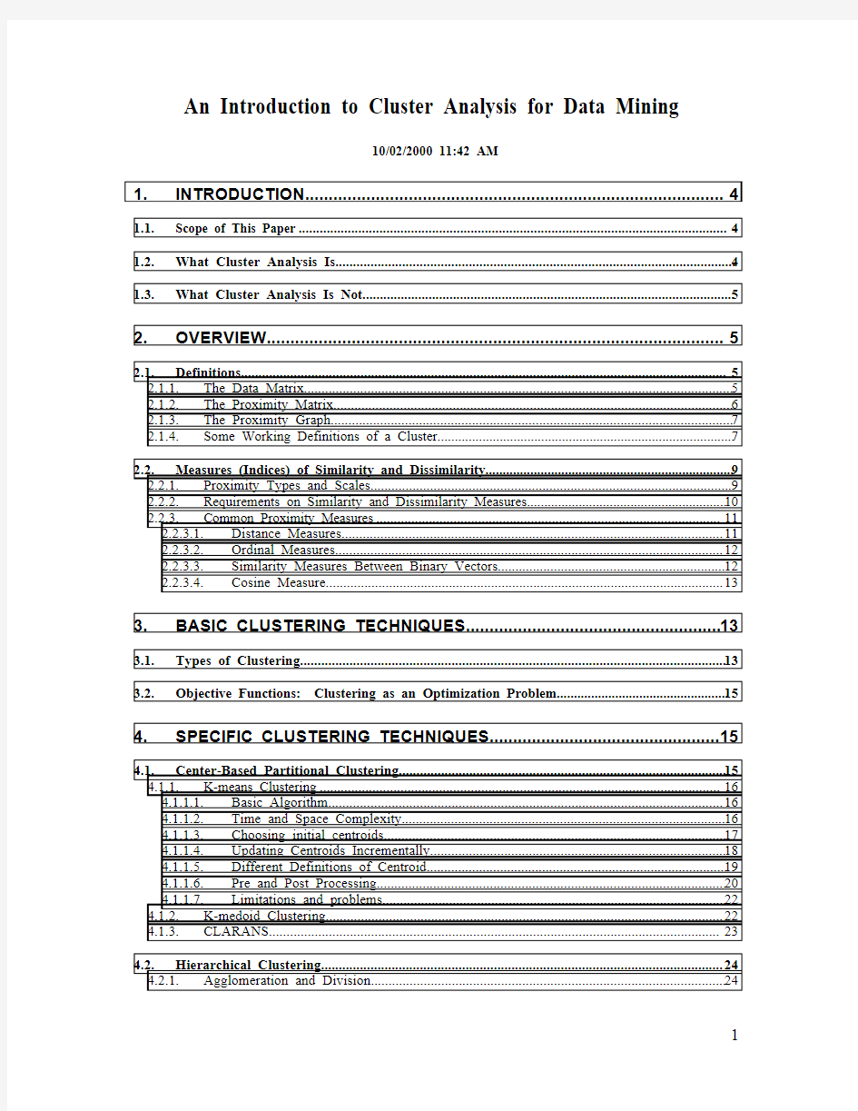
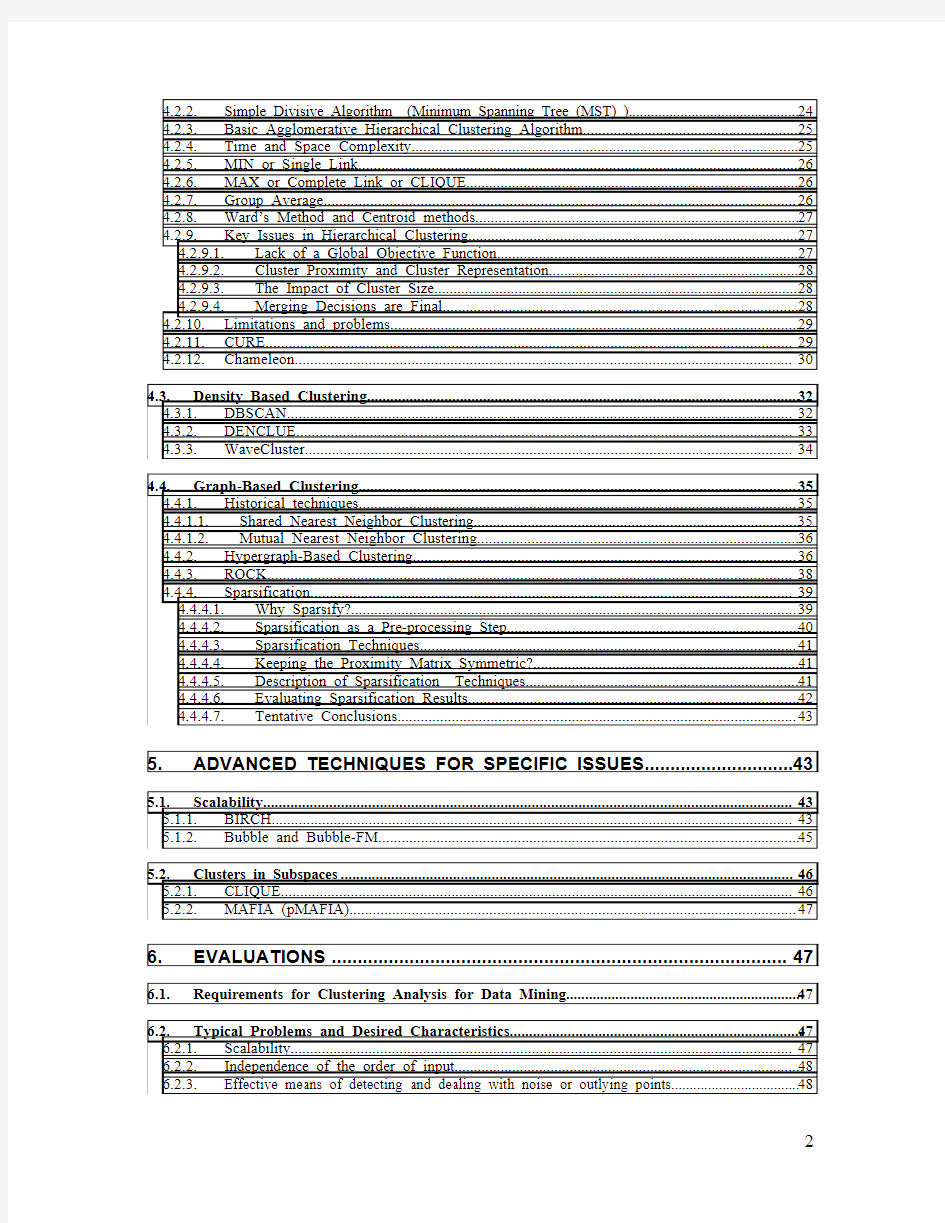
2.1.2. The Proximity Matrix
While cluster analysis sometimes uses the original data matrix, many clustering algorithms use a similarity matrix, S, or a dissimilarity matrix, D. For convenience, both matrices are commonly referred to as a proximity matrix, P. A proximity matrix, P, is an m by m matrix containing all the pairwise dissimilarities or similarities between the objects being considered. If x i and x j are the i th and j th objects, respectively, then the entry
at the i th row and j th column of the proximity matrix is the similarity, s ij , or the dissimilarity, d ij , between x i and x j . For simplicity, we will use p ij to represent either s ij or d ij . Figure 2 shows four points and the corresponding data and proximity (distance) matrices. More examples of dissimilarity and similarity will be provided shortly. point x y p1 0 2 p2 2 0 p3 3 1 p4 5 1
p1 p2 p3 p4 p1 0.000 2.828 3.162 5.099 p2 2.828 0.000 1.414 3.162 p3 3.162 1.414 0.000 2.000 p4 5.099 3.162 2.000 0.000 Figure 2. Four points and their corresponding data and proximity (distance) matrices.
For completeness, we mention that objects are sometimes represented by more complicated data structures than vectors of attributes, e.g., character strings. Determining the similarity (or differences) of two objects in such a situation is more complicated, but if a reasonable similarity (dissimilarity) measure exists, then a clustering analysis can still be performed. In particular, clustering techniques that use a proximity matrix are unaffected by the lack of a data matrix.
2.1.
3. The Proximity Graph
A proximity matrix defines a weighted graph, where the nodes are the points being clustered, and the weighted edges represent the proximities between points, i.e., the entries of the proximity matrix. While this proximity graph can be directed, which corresponds to an asymmetric proximity matrix, most clustering methods assume an undirected graph. Relaxing the symmetry requirement can be useful for clustering or pattern recognition, but we will assume undirected proximity graphs (symmetric proximity matrices) in our discussions.
From a graph point of view, clustering is equivalent to breaking the graph into connected components, one for each cluster. Likewise, many issues related to clustering can be cast in graph-theoretic terms, e.g., the issues of cluster cohesion and the degree of coupling with other clusters can be measured by the number and strength of links between and within clusters. Also, many clustering techniques, e.g., minimum spanning tree (section 4.2.1), single link (section 4.2.5), and complete link (section 4.2.6), are most Some clustering algorithms, e.g., Chameleon (section 4.2.12), first sparsify the the links of the proximity graph. (This corresponds to setting a proximity matrix entry to 0 or ∞, depending on whether we are using similarities or dissimilarities, respectively.) See section 4.4.4 for details.
2.1.4. Some Working Definitions of a Cluster
As mentioned above, the term, cluster, does not have a precise definition. However, several working definitions of a cluster are commonly used.
1) Well-Separated Cluster Definition: A cluster is a set of points such that any point in
a cluster is closer (or more similar) to every other point in the cluster than to any
point not in the cluster. Sometimes a threshold is used to specify that all the points in
a cluster must be sufficiently close (or similar) to one another.
Figure 3: Three well-separated clusters of 2 dimensional points.
However, in many sets of data, a point on the edge of a cluster may be closer (or more similar) to some objects in another cluster than to objects in its own cluster.
Consequently, many clustering algorithms use the following criterion.
2) Center-based Cluster Definition: A cluster is a set of objects such that an object in a
cluster is closer (more similar) to the “center” of a cluster, than to the center of any other cluster. The center of a cluster is often a centroid, the average of all the points in the cluster, or a medoid, the most “representative” point of a cluster.
Figure 4: Four center-based clusters of 2 dimensional points.
3) Contiguous Cluster Definition (Nearest neighbor or Transitive Clustering): A
cluster is a set of points such that a point in a cluster is closer (or more similar) to one or more other points in the cluster than to any point not in the cluster.
Figure 5: Eight contiguous clusters of 2 dimensional points.
4) Density-based definition: A cluster is a dense region of points, which is separated by low-density regions, from other regions of high density. This definition is more often used when the clusters are irregular or intertwined, and when noise and outliers are present. Note that the contiguous definition would find only one cluster in figure 6. Also note that the three curves don’t form clusters since they fade into the noise, as does the bridge between the two small circular clusters.
Figure 6: Six dense clusters of 2 dimensional points.
5) Similarity-based Cluster definition: A cluster is a set of objects that are “similar”,
and objects in other clusters are not “similar.” A variation on this is to define a cluster as a set of points that together create a region with a uniform local property, e.g., density or shape.
2.2. Measures (Indices) of Similarity and Dissimilarity
2.2.1. Proximity Types and Scales
The attributes of the objects (or their pairwise similarities and dissimilarities) can be of different data types and can be measured on different data scales.
The different types of attributes are
1) Binary(two values)
2) Discrete(a finite number of values)
3) Continuous(an effectively infinite number of values)
The different data scales are
1) Qualitative
a) Nominal – the values are just different names.
Example 1: Zip Codes
Example 2: Colors: white, black, green, red, yellow, etc.
Example 3: Sex: male, female
Example 4: 0 and 1 when they represent Yes and No.
b) Ordinal – the values reflect an ordering, nothing more.
Example 1: Good, Better, Best
Example 2: Colors ordered by the spectrum.
Example 3: 0 and 1 are often considered to be ordered when used as Boolean
values (false/true), with 0 < 1.
2) Quantitative
a) Interval – the difference between values is meaningful, i.e., a unit of
measurement exits.
Example 1: On a scale of 1 to 10 rate the following potato chips.
b) Ratio – the scale has an absolute zero so that ratios are meaningful.
Example 1: The height, width, and length of an object.
Example 2: Monetary quantities, e.g., salary or profit.
Example 3: Many physical quantities like electrical current, pressure, etc.
Data scales and types are important since the type of clustering used often depends on the data scale and type.
2.2.2. Requirements on Similarity and Dissimilarity Measures
Proximities are normally subject to a number of requirements [DJ88]. We list these below. Recall that p ij is the proximity between points, x i and x j.
1) (a) For a dissimilarity: p ii= 0 for all i. (Points aren’t different from themselves.)
(b) For a similarity: p ii> max p ij(Points are most similar to themselves.)
(Similarity measures are often required to be between 0 and 1, and in that case
p ii= 1, is the requirement.)
2) p ij= p ji (Symmetry)
This implies that the proximity matrix is symmetric. While this is typical, it is not
always the case. An example is a confusion matrix, which implicitly defines a
similarity between entities that is measured by how often various entities, e.g.,
characters, are misclassified as one another. Thus, while 0’s and O’s are confused
with each other, it is not likely that 0’s are mistaken for O’s at the same rate that O’s are mistaken for 0’s.
3) p ij> 0 for all i and j (Positivity)
Additionally, if the proximity measure is real-valued and is a true metric in a mathematical sense, then the following two conditions also hold in addition to conditions 2 and 3.
4) p ij= 0 only if i = j.
5) p ik p ij+ p jk for all i, j, k. (Triangle inequality.)
Dissimilarities that satisfy conditions 1-5 are called distances, while “dissimilarity” is a term commonly reserved for those dissimilarities that satisfy only conditions 1-3.
2.2.
3. Common Proximity Measures
2.2.
3.1. Distance Measures
The most commonly used proximity measure, at least for ratio scales (scales with an absolute 0) is the Minkowski metric, which is a generalization of the normal distance between points in Euclidean space. It is defined as
where, r is a parameter, d is the dimensionality of the data object, and x ik and x jk are, respectively, the k th components of the i th and j th objects, x i and x j .
The following is a list of the common Minkowski distances for specific values of r .
1) r = 1. City block (Manhattan, taxicab, L 1 norm) distance.
A common example of this is the Hamming distance, which is just the number of bits that are different between two binary vectors.
2) r = 2. Euclidean distance. The most common measure of the distance between two points.
3) r → ∞. “supremum” (L max norm, L ∞ norm) distance.
This is the maximum difference between any component of the vectors.
Figure 7 gives the proximity matrices for L1, L2 and L ∞ , respectively using the given data matrix which we copied from an earlier example.
point x y
p1 0 2
p2 2 0
p3 3 1
p4 5 1
L1 p1 p2 p3 p4
p1 0.000 4.000 4.000 6.000
p2 4.000 0.000 2.000 4.000
p3 4.000 2.000 0.000 2.000
p4 6.000 4.000 2.000 0.000 L2 p1 p2 p3 p4 p1 0.000 2.828 3.162 5.099 p2 2.828 0.000 1.414 3.162 p3 3.162 1.414 0.000 2.000 p4 5.099 3.162 2.000 0.000 L ∞ p1 p2 p3 p4 p1 0.000 2.000 3.000 5.000 p2 2.000 0.000 1.000 3.000 p3 3.000 1.000 0.000 2.000 p4 5.000 3.000 2.000 0.000 Figure 7. Data matrix and the L1, L2, and L ∞ proximity matrices.
The r parameter should not be confused with the dimension, d . For example, Euclidean, Manhattan and supremum distances are defined for all values of d , 1, 2, 3, …, and specify different ways of combining the differences in each dimension (attribute) into an overall distance.
r
r d k jk ik ij x x p /11÷÷????è??=?=
2.2.
3.2. Ordinal
Measures
Another common type of proximity measure is derived by ranking the distances between pairs of points from 1 to m * (m - 1) / 2. This type of measure can be used with most types of data and is often used with a number of the hierarchical clustering algorithms that are discussed in section 4.2. Figure 8 shows how the L2 proximity matrix
L2 p1 p2 p3 p4 p1 0.000 2.828 3.162 5.099 p2 2.828 0.000 1.414 3.162 p3 3.162 1.414 0.000 2.000 p4 5.099 3.162 2.000 0.000 ordinal
p1 p2 p3 p4 p1 0 3 4 5 p2 3 0 1 4 p3 4 1 0 2 p4 5 4 2 0
Figure 8. An L2 proximity matrix and the corresponding ordinal proximity matrix.
2.2.
3.3. Similarity Measures Between Binary Vectors
There are many measures of similarity between binary vectors. These measures are referred to as similarity coefficients, and have values between 0 and 1. A value of 1 indicates that the two vectors are completely similar, while a value of 0 indicates that the vectors are not at all similar. There are many rationales for why one coefficient is better than another in specific instances [DJ88, KR90], but we will mention only a few.
The comparison of two binary vectors, p and q, leads to four quantities:
M01 = the number of positions where p was 0 and q was 1
M10 = the number of positions where p was 1 and q was 0
M00 = the number of positions where p was 0 and q was 0
M11 = the number of positions where p was 1 and q was 1
The simplest similarity coefficient is the simple matching coefficient
SMC = (M11 + M00) / (M01 + M10 + M11 + M00)
Another commonly used measure is the Jaccard coefficient.
J = (M11) / (M01 + M10 + M11)
Conceptually, SMC equates similarity with the total number of matches, while J considers only matches on 1’s to be important. It is important to realize that there are situations in which both measures are more appropriate.
For example, consider the following pairs of vectors and their simple matching and Jaccard similarity coefficients
a = 1 0 0 0 0 0 0 0 0 0 SMC = .8
b = 0 0 0 0 0 0 1 0 0 1J = 0
If the vectors represent student’s answers to a True-False test, then both 0-0 and 1-1 matches are important and these two students are very similar, at least in terms of the grades they will get.
Suppose instead that the vectors indicate whether 10 particular items are in the “market baskets” of items purchased by two shoppers. Then the Jaccard measure is a more appropriate measure of similarity since it would be very odd to say that two market baskets that don’t contain any similar items are the same. For calculating the similarity of market baskets, and in many other cases, the presence of an item is far more important than absence of an item.
Measure
2.2.
3.
4. Cosine
For purposes of information retrieval, e.g., as in Web search engines, documents are often stored as vectors, where each attribute represents the frequency with which a particular term (word) occurs in the document. (It is much more complicated than this, of course, since certain common words are ignored and normalization is performed to account for different forms of the same word, document length, etc.) Such vectors can have thousands or tens of thousands of attributes.
If we wish to compare the similarity of two documents, then we face a situation much like that in the previous section, except that the vectors are not binary vectors. However, we still need a measure like the Jaccard measure, which ignores 0-0 matches. The motivation is that any two documents are likely to “not contain” many of the same words, and thus, if 0-0 matches are counted most documents will be highly similar to most other documents. The cosine measure, defined below, is the most common measure of document similarity. If d1 and d2 are two document vectors, then
cos( d1, d2 ) = (d1?d2) / ||d1|| ||d2|| ,
where ? indicates vector dot product and ||d|| is the length of vector d.
For example,
d1= 3 2 0 5 0 0 0 2 0 0
d2 = 1 0 0 0 0 0 0 1 0 2
d1?d2= 3*1 + 2*0 + 0*0 + 5*0 + 0*0 + 0*0 + 0*0 + 2*1 + 0*0 + 0*2 = 5
||d1|| = (3*3 + 2*2 + 0*0 + 5*5 + 0*0 +0*0 + 0*0 + 2*2 + 0*0 + 0*0)0.5 = 6.480
||d2|| = (1*1 + 0*0 + 0*0 + 0*0 + 0*0 + 0*0 + 0*0 + 1*1 + 0*0 + 2*2) 0.5 = 2.236
cos( d1, d2 ) = .31
3. Basic Clustering Techniques
3.1. Types of Clustering
Many different clustering techniques that have been proposed over the years. These techniques can be described using the following criteria [DJ88]:
1) Hierarchical vs. partitional (nested and unnested). Hierarchical techniques
produce a nested sequence of partitions, with a single, all inclusive cluster at the top
and singleton clusters of individual points at the bottom. Each intermediate level can be viewed as combining (splitting) two clusters from the next lower (next higher) level. (While most hierarchical algorithms involve joining two clusters or splitting a cluster into two sub-clusters, some hierarchical algorithms join more than two clusters in one step or split a cluster into more than two sub-clusters.)
The following figures indicate different ways of graphically viewing the hierarchical clustering process. Figures 9a and 9b illustrate the more “traditional” view of hierarchical clustering as a process of merging two clusters or splitting one cluster into two. Figure 9a gives a “nested set” representation of the process, while Figure 9b shows a “tree’ representation, or dendogram. Figure 9c and 9d show a different, hierarchical clustering, one in which points p1 and p2 are grouped together in the same step that also groups points p3 and p4 together.
Figure 9a . Traditional nested set. Figure 9b . Traditional dendogram Figure 9c. Non-traditional nested set Figure 9d. Non-traditional dendogram.
Partitional techniques create a one-level (unnested) partitioning of the data points. If K is the desired number of clusters, then partitional approaches typically find all K clusters at once. Contrast this with traditional hierarchical schemes, which bisect a cluster to get two clusters or merge two clusters to get one. Of course, a hierarchical approach can be used to generate a flat partition of K clusters, and likewise, the repeated application of a partitional scheme can provide a hierarchical clustering.
p4
p1p2p3 p4
p1p2p3
2) Divisive vs. agglomerative. Hierarchical clustering techniques proceed either from
the top to the bottom or from the bottom to the top, i.e., a technique starts with one large cluster and splits it, or starts with clusters each containing a point, and then merges them.
3) Incremental or non-incremental. Some clustering techniques work with an item at
a time and decide how to cluster it given the current set of points that have already
been processed. Other techniques use information about all the points at once. Non-incremental clustering algorithms are far more common.
3.2. Objective Functions: Clustering as an Optimization Problem
Many clustering techniques are based on trying to minimize or maximize a global objective function. The clustering problem then becomes an optimization problem, which, in theory, can be solved by enumerating all possible ways of dividing the points into clusters and evaluating the “goodness” of each potential set of clusters by using the given objective function. Of course, this “exhaustive” approach is computationally infeasible (NP complete) and as a result, a number of more practical techniques for optimizing a global objective function have been developed.
One approach to optimizing a global objective function is to rely on algorithms, which find solutions that are often good, but not optimal. An example of this approach is the K-means clustering algorithm (section 4.1.1) which tries to minimize the sum of the Another approach is to fit the data to a model. An example of such techniques is mixture models (section 7.1.1), which assume that the data is a “mixture” of a number of underlying statistical distributions. These clustering algorithms seek to find a solution to a clustering problem by finding the maximum likelihood estimate for the statistical parameters that describe the clusters.
Still another approach is to forget about global objective functions. In particular, hierarchical clustering procedures proceed by making local decisions at each step of the clustering process. These ‘local’ or ‘per-step’ decisions are also based on an objective function, but the overall or global result is not easily interpreted in terms of a global objective function This will be discussed further in one of the sections on hierarchical clustering techniques (section 4.2.9).
4. Specific Clustering Techniques
4.1. Center-Based Partitional Clustering
As described earlier, partitional clustering techniques create a one-level partitioning of the data points. There are a number of such techniques, but we shall only describe two approaches in this section: K-means (section 4.1.1) and K-medoid (section 4.1.2).
Both these techniques are based on the idea that a center point can represent a cluster. For K-means we use the notion of a centroid, which is the mean or median point of a group of points. Note that a centroid almost never corresponds to an actual data point. For K-medoid we use the notion of a medoid, which is the most representative
(central) point of a group of points. By its definition a medoid is required to be an actual data point.
Section 4.1.3 introduces CLARANS, a more efficient version of the basic
clustering methods for data mining that are based on center-based partitional approaches. (BIRCH is more like K-means and Bubble is more like K-medoid.) However, both of BIRCH and Bubble use a wide variety of techniques to help enhance their scalability, i.e., their ability to handle large data sets, and consequently, their discussion is postponed to sections 5.1.1 and section 5.1.2, respectively.
4.1.1. K-means Clustering
4.1.1.1. Basic
Algorithm
The K-means clustering technique is very simple and we immediately begin with a description of the basic algorithm. We elaborate in the following sections.
Basic K-means Algorithm for finding K clusters.
1. Select K points as the initial centroids.
2. Assign all points to the closest centroid.
3. Recompute the centroid of each cluster.
4. Repeat steps 2 and 3 until the centroids don’t change.
In the absence of numerical problems, this procedure always converges to a solution, although the solution is typically a local minimum. The following diagram gives an example of this. Figure 10a shows the case when the cluster centers coincide with the circle centers. This is a global minimum. Figure 10b shows a local minima.
Figure 10a. A globally minimal clustering solution
Figure 10b. A locally minimal clustering solution.
4.1.1.2. Time and Space Complexity
Since only the vectors are stored, the space requirements are basically O(mn), where m is the number of points and n is the number of attributes. The time requirements are O(I*K*m*n), where I is the number of iterations required for convergence. I is typically small (5-10) and can be easily bounded as most changes occur in the first few
iterations. Thus, K-means is linear in m, the number of points, and is efficient, as well as simple, as long as the number of clusters is significantly less than m.
4.1.1.3. Choosing initial centroids
Choosing the proper initial centroids is the key step of the basic K-means procedure. It is easy and efficient to choose initial centroids randomly, but the results are often poor. It is possible to perform multiple runs, each with a different set of randomly chosen initial centroids – one study advocates 30 - but this may still not work depending on the data set and the number of clusters sought.
We start with a very simple example of three clusters and 16 points. Figure 11a indicates the “natural” clustering that results when the initial centroids are “well” distributed. Figure 11b indicates a “less natural” clustering that happens when the initial centroids are poorly chosen.
Figure 11a: Good starting centroids and a “natural” clustering.
Figure 11b: Bad starting centroids and a “less natural” clustering.
We have also constructed the artificial data set, shown in figure 12a as another illustration of what can go wrong. The figure consists of 10 pairs of circular clusters, where each cluster of a pair of clusters is close to each other, but relatively far from the other clusters. The probability that an initial centroid will come from any given cluster is 0.10, but the probability that each cluster will have exactly one initial centroid is 10!/1010
= 0.00036. (Technical note: This assumes sampling with replacement, i.e., that two initial centroids could be the same point.)
There isn’t any problem as long as two initial centroids fall anywhere in a pair of clusters, since the centroids will redistribute themselves, one to each cluster, and so achieve a globally minimal error,. However, it is very probable that one pair of clusters will have only one initial centroid. In that case, because the pairs of clusters are far apart, the K-means algorithm will not redistribute the centroids between pairs of clusters, and thus, only a local minima will be achieved. When starting with an uneven distribution of initial centroids as shown in figure 12b, we get a non-optimal clustering, as is shown in figure 12c, where different fill patterns indicate different clusters. One of the clusters is split into two clusters, while two clusters are joined in a single cluster.
Figure 12a: Data distributed in 10 circular regions
Figure 12b: Initial Centroids
Figure 12c: K-means clustering result
Because random sampling may not cover all clusters, other techniques are often used for finding the initial centroids. For example, initial centroids are often chosen from dense regions, and so that they are well separated, i.e., so that no two centroids are chosen from the same cluster.
4.1.1.4. Updating Centroids Incrementally
Instead of updating the centroid of a cluster after all points have been assigned to clusters, the centroids can be updated as each point is assigned to a cluster. In addition, the relative weight of the point being added may be adjusted. The goal of these modifications is to achieve better accuracy and faster convergence. However, it may be difficult to make a good choice for the relative weight. These update issues are similar to those of updating weights for artificial neural nets.
Incremental update also has another advantage – empty clusters are not produced. (All clusters start with a single point and if a cluster ever gets down to one point, then that point will always be reassigned to that cluster.) Empty clusters are often observed when centroid updates are performed only after all points have been assigned to clusters.
This imposes the need for a technique to choose a new centroid for an empty cluster, for otherwise the squared error will certainly be larger than it would need to be. A common approach is to choose as the new centroid the point that is farthest away from any current center. If nothing else, this eliminates the point that currently contributes the most to the squared error.
Updating points incrementally may introduce an order dependency problem, which can be ameliorated by randomizing the order in which the points are processed. However, this is not really feasible unless the points are in main memory. Updating the centroids after all points are assigned to clusters results in order independence approach.
Finally, note that when centers are updated incrementally, each step of the process may require updating two centroids if a point switches clusters. However, K-means tends to converge rather quickly and so the number of points switching clusters will tend to be small after a few passes over all the points.
4.1.1.
5. Different Definitions of Centroid
The K-means algorithm is derived by asking how we can obtain a partition of the data into K clusters such that the sum of the squared distance of a point from the “center” of the cluster is minimized. In mathematical terms we seek to minimize
Error = ??=∈?K 1i C x 2i i c x H H H = ???=∈=?K i C x d j ij j i c x 11
2)(H where x H is a vector (point) and i c H is the “center” of the cluster, d is the dimension of x H and i c H and x j and c ij are the components of x H and i c H .)
We can solve for the p th cluster,p c H , by solving for each component, c pk , 1 ≤ k ≤ d by differentiating the Error , setting it to 0, and solving as the following equations indicate.
???=∈=???=??K
i C x d j ij j pk pk i c x c Error c 11
2)(H ???=∈=???=
K i C x d
j ij j pk i c x c 112)(H ?∈=?=p C x pk k c x H 0)(*2 ???∈∈∈=
T=T=?p p p C x k p pk C x k pk p C x pk k x n c x c n c x H H H 1
0)(*2 Thus, we find that ?∈=p C x p x c H H H p n 1, the mean of the points in the cluster. This is
pleasing since it agrees with our intuition of what the center of a cluster should be.
However, we can instead ask how we can obtain a partition of the data into K clusters such that the sum of the distance of a point from the “center” of the cluster is minimized. In mathematical terms, we now seek to minimize the equation
Error = ??=∈?K 1i C x i i
c x H H H
This problem has been extensively studied in operations research under the name of the multi-source Weber problem [Ta98] and has obvious applications to the location of warehouses and other facilities that need to be centrally located. We leave it as an exercise to the reader to verify that the centroid in this case is still the mean.
Finally, we can instead ask how we can obtain a partition of the data into K clusters such that the sum of the L1 distance of a point from the “center” of the cluster is minimized. In mathematical terms, we now seek to minimize the equation
Error = ???=∈=?K 1i C x i H d
1j ij j c x We can solve for the p th cluster,p c H , by solving for each component, c pk , 1 ≤ k ≤ d
by differentiating the Error , setting it to 0, and solving as the following equations indicate.
???=∈=???=??K
i C x d j ij j pk pk i c x c Error c 11H . ???=∈=???=K i C x d j ij j pk i
c x c 11H . 01=???=
??∈=p C x d j pk k pk c x c H .
0)(01=?T=??????∈∈=p p C x pk k C x d j pk k pk
c x sign c x c H H Thus, if we solve for p c H , we fin
d that ()p p C x c ∈=H H median , th
e point whose coordinates are the median values o
f the correspondin
g coordinate values of the points in the cluster. While the median of a group of points is straightforward to compute, this computation is not as efficient as the calculation of a mean.
In the first case we say we are attempting to minimize the within cluster squared error, while in the second case and third cases we just say that we are attempting to minimize the absolute within cluster error, where the error may either the L1 or L2 distance.
4.1.1.6. Pre and Post Processing
Sometimes the quality of the clusters that are found can be improved by pre-processing the data. For example, when we use the squared error criteria, outliers can