东南大学matlab第三次大作业
- 格式:doc
- 大小:2.92 MB
- 文档页数:14
数值分析大作业三四五六七数值分析大作业三四五六七Document number【SA80SAB-SAA9SYT-SAATC-SA6UT-SA18】大作业三1. 给定初值0x 及容许误差,编制牛顿法解方程f (x )=0的通用程序. 解:Matlab 程序如下:函数m 文件:fu.mfunction Fu=fu(x)Fu=x^3/3-x;end函数m 文件:dfu.mfunction Fu=dfu(x)Fu=x^2-1;end用Newton 法求根的通用程序Newton.mclear;x0=input('请输入初值x0:');ep=input('请输入容许误差:');flag=1;while flag==1x1=x0-fu(x0)/dfu(x0);if abs(x1-x0)<ep< p="">flag=0;endx0=x1;endfprintf('方程的一个近似解为:%f\n',x0);寻找最大δ值的程序:Find.mcleareps=input('请输入搜索精度:');ep=input('请输入容许误差:');flag=1;k=0;x0=0;while flag==1sigma=k*eps;x0=sigma;k=k+1;m=0;flag1=1;while flag1==1 && m<=10^3x1=x0-fu(x0)/dfu(x0);if abs(x1-x0)endm=m+1;x0=x1;endif flag1==1||abs(x0)>=epflag=0;endendfprintf('最大的sigma 值为:%f\n',sigma);2.求下列方程的非零根5130.6651()ln 05130.665114000.0918x x f x x +??=-= ?-解:Matlab 程序为:(1)主程序clearclcformat longx0=765;N=100;errorlim=10^(-5);x=x0-f(x0)/subs(df(),x0);n=1;while n<n< p="">x=x0-f(x0)/subs(df(),x0);if abs(x-x0)>errorlimn=n+1;elsebreak;endx0=x;enddisp(['迭代次数: n=',num2str(n)])disp(['所求非零根: 正根x1=',num2str(x),' 负根x2=',num2str(-x)])(2)子函数非线性函数ffunction y=f(x)y=log((513+0.6651*x)/(513-0.6651*x))-x/(1400*0.0918);end(3)子函数非线性函数的一阶导数dffunction y=df()syms x1y=log((513+0.6651*x1)/(513-0.6651*x1))-x1/(1400*0.0918);y=diff(y);end运行结果如下:迭代次数: n=5所求非零根: 正根x1=767.3861 负根x2=-767.3861大作业四试编写MATLAB 函数实现Newton 插值,要求能输出插值多项式. 对函数21()14f x x=+在区间[-5,5]上实现10次多项式插值.分析:(1)输出插值多项式。
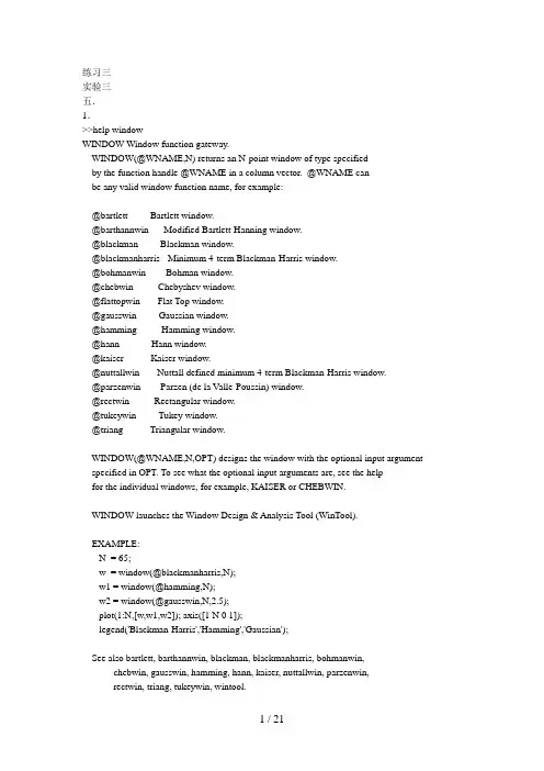
练习三实验三五.1.>>help windowWINDOW Window function gateway.WINDOW(@WNAME,N) returns an N-point window of type specifiedby the function handle @WNAME in a column vector. @WNAME canbe any valid window function name, for example:@bartlett - Bartlett window.@barthannwin - Modified Bartlett-Hanning window.@blackman - Blackman window.@blackmanharris - Minimum 4-term Blackman-Harris window.@bohmanwin - Bohman window.@chebwin - Chebyshev window.@flattopwin - Flat Top window.@gausswin - Gaussian window.@hamming - Hamming window.@hann - Hann window.@kaiser - Kaiser window.@nuttallwin - Nuttall defined minimum 4-term Blackman-Harris window.@parzenwin - Parzen (de la Valle-Poussin) window.@rectwin - Rectangular window.@tukeywin - Tukey window.@triang - Triangular window.WINDOW(@WNAME,N,OPT) designs the window with the optional input argument specified in OPT. To see what the optional input arguments are, see the helpfor the individual windows, for example, KAISER or CHEBWIN.WINDOW launches the Window Design & Analysis Tool (WinTool).EXAMPLE:N = 65;w = window(@blackmanharris,N);w1 = window(@hamming,N);w2 = window(@gausswin,N,2.5);plot(1:N,[w,w1,w2]); axis([1 N 0 1]);legend('Blackman-Harris','Hamming','Gaussian');See also bartlett, barthannwin, blackman, blackmanharris, bohmanwin,chebwin, gausswin, hamming, hann, kaiser, nuttallwin, parzenwin,rectwin, triang, tukeywin, wintool.Overloaded functions or methods (ones with the same name in other directories) help fdesign/window.mReference page in Help browser doc window 2.>>N = 128;w = window(@rectwin,N); w1 = window(@bartlett,N); w2 = window(@hamming,N);plot(1:N,[w,w1,w2]); axis([1 N 0 1]); legend('矩形窗','Bartlett','Hamming');2040608010012000.10.20.30.40.50.60.70.80.913.>>wvtool(w,w1,w2)六.ts=0.01;N=20;t=0:ts:(N-1)*ts;x=2*sin(4*pi*t)+5*cos(6*pi*t);g=fft(x,N);y=abs(g)/100;figure(1):plot(0:2*pi/N:2*pi*(N-1)/N,y); grid;01234560.050.10.150.20.250.30.350.40.45ts=0.01; N=30;t=0:ts:(N-1)*ts;x=2*sin(4*pi*t)+5*cos(6*pi*t); g=fft(x,N); y=abs(g)/100;figure(2):plot(0:2*pi/N:2*pi*(N-1)/N,y); grid;012345670.10.20.30.40.50.60.7ts=0.01; N=50;t=0:ts:(N-1)*ts;x=2*sin(4*pi*t)+5*cos(6*pi*t); g=fft(x,N); y=abs(g)/100;figure(3):plot(0:2*pi/N:2*pi*(N-1)/N,y); grid;123456700.10.20.30.40.50.60.70.80.91ts=0.01; N=100;t=0:ts:(N-1)*ts;x=2*sin(4*pi*t)+5*cos(6*pi*t); g=fft(x,N); y=abs(g)/100;figure(4):plot(0:2*pi/N:2*pi*(N-1)/N,y); grid;012345670.511.522.5ts=0.01; N=150;t=0:ts:(N-1)*ts;x=2*sin(4*pi*t)+5*cos(6*pi*t); g=fft(x,N); y=abs(g)/100;figure(5):plot(0:2*pi/N:2*pi*(N-1)/N,y); grid;012345670.511.522.53实验八 1.%冲激响应 >> clear; b=[1,3]; a=[1,3,2]; sys=tf(b,a); impulse(sys); 结果:Impulse ResponseTime (sec)A m p l i t u d e%求零输入响应 >> A=[1,3;0,-2]; B=[1;2]; Q=A\B Q = 4-1>> clear B=[1,3]; A=[1,3,2];[a,b,c,d]=tf2ss(B,A) sys=ss(a,b,c,d); x0=[4;-1]; initial(sys,x0); grid; a =-3 -2 1 0 b =1 0 c =1 3 d = 001234560.20.40.60.811.21.4Response to Initial ConditionsTime (sec)A m p l i t u d e2.%冲激响应 >> clear; b=[1,3]; a=[1,2,2]; sys=tf(b,a); impulse(sys)Impulse ResponseTime (sec)A m p l i t u d e%求零输入响应 >> A=[1,3;1,-2]; B=[1;2]; Q=A\B Q =1.6000 -0.2000 >> clear B=[1,3]; A=[1,2,2];[a,b,c,d]=tf2ss(B,A) sys=ss(a,b,c,d); x0=[1.6;-0.2]; initial(sys,x0); grid; a =-2 -2 1 0 b = 10 c =1 3 d = 0Response to Initial ConditionsTime (sec)A m p l i t u d e3.%冲激响应 >> clear; b=[1,3]; a=[1,2,1]; sys=tf(b,a); impulse(sys)Impulse ResponseTime (sec)A m p l i t u d e%求零输入响应 >> A=[1,3;1,-1]; B=[1;2]; Q=A\B Q =1.7500 -0.2500>> clear B=[1,3]; A=[1,2,1];[a,b,c,d]=tf2ss(B,A) sys=ss(a,b,c,d); x0=[1.75;-0.25]; initial(sys,x0); grid; a =-2 -1 1 0 b =1 0 c =1 3 d = 00510150.20.40.60.811.21.41.6Response to Initial ConditionsTime (sec)A m p l i t u d e二. >> clear; b=1;a=[1,1,1,0]; sys=tf(b,a); subplot(2,1,1);impulse(sys);title('冲击响应'); subplot(2,1,2);step(sys);title('阶跃响应'); t=0:0.01:20; e=sin(t);r=lsim(sys,e,t); figure;subplot(2,1,1);plot(t,e);xlabel('Time');ylabel('A');title('激励信号'); subplot(2,1,2);plot(t,r);xlabel('Time');ylabel('A');title('响应信号');024681012141618200.511.5冲击响应Time (sec)A m p l i t u d e024681012141618205101520阶跃响应Time (sec)A m p l i t u d e02468101214161820-1-0.500.51Time A激励信号2468101214161820-10123TimeA响应信号三. 1.>> clear; b=[1,3]; a=[1,3,2]; t=0:0.08:8; e=[exp(-3*t)]; sys=tf(b,a); lsim(sys,e,t);0.10.20.30.40.50.60.70.80.91Linear Simulation ResultsTime (sec)A m p l i t u d e2.>> clear; b=[1,3]; a=[1,2,2]; t=0:0.08:8; sys=tf(b,a); step(sys)0.20.40.60.811.21.41.6Step ResponseTime (sec)A m p l i t u d e3.>> clear; b=[1,3]; a=[1,2,1]; t=0:0.08:8; e=[exp(-2*t)]; sys=tf(b,a); lsim(sys,e,t);0.10.20.30.40.50.60.70.80.91Linear Simulation ResultsTime (sec)A m p l i t u d eDoc: 1.>> clear; B=[1]; A=[1,1,1]; sys=tf(B,A,-1); n=0:200;e=5+cos(0.2*pi*n)+2*sin(0.7*pi*n); r=lsim(sys,e); stem(n,r);0204060801001201401601802002.>> clear;B=[1,1,1];A=[1,-0.5,-0.5];sys=tf(B,A,-1);e=[1,zeros(1,100)];n=0:100;r=lsim(sys,e);stem(n,r);010203040506070809010021 / 21。
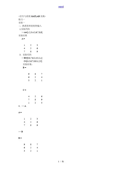
<信号与系统MATLAB实践> 练习一实验一二. 熟悉简单的矩阵输入1.实验代码>>A=[1,2,3;4,5,6;7,8,9]实验结果A =1 2 34 5 67 8 93.实验代码>>B=[9,8,7;6,5,4;3,2,1]C=[4,5,6;7,8,9;1,2,3]实验结果:B =9 8 76 5 43 2 1C =4 5 67 8 91 2 3 4.>> AA =1 2 34 5 67 8 9>> BB =9 8 76 5 43 2 1C =4 5 67 8 91 2 3三. 根本序列运算1.>>A=[1,2,3],B=[4,5,6]A =1 2 3B =4 5 6 >> C=A+BC =5 7 9 >> D=A-BD =-3 -3 -3 >> E=A.*BE =4 10 18 >> F=A./BF =>> G=A.^B1 32 729 >> stem(A)>>stem(B)>> stem(D)>> stem(F)再举例:>> a=[-1,-2,-3] a =-1 -2 -3 >> b=[-4,-5,-6]b =-4 -5 -6 >> c=a+bc =-5 -7 -9 >> d=a-bd =3 3 3 >> e=a.*be =4 10 18 >> f=a./bf =>> g=a.^bg =>> stem(a)>> stem(c)>> stem(e)>> stem(g)2. >>t=0:0.001:10f=5*exp(-t)+3*exp(-2*t);plot(t,f)ylabel('f(t)');xlabel('t');title('(1)');>> t=0:0.001:3;f=(sin(3*t))./(3*t);plot(t,f)ylabel('f(t)');xlabel('t');title('(2)');>> k=0:1:4;f=exp(k); 1 1.52 2.53 3.54 4.550102030405060四. 利用MATLAB求解线性方程组2.>>A=[1,1,1;1,-2,1;1,2,3]b=[2;-1;-1]x=inv(A)*bA =1 1 11 -2 11 2 3b =2-1-1x =4.>> A=[2,3,-1;3,-2,1;1,2,1]b=[18;8;24]x=inv(A)*bA =2 3 -13 -2 11 2 1b =18824x =468实验二二.1.>> k=0:50x=sin(k);stem(x)xlabel('k');ylabel('sinX');title('sin(k)ε(k)');2.>> k=-25:1:25x=sin(k)+sin(pi*k); stem(k,x)xlabel('k');ylabel('f(k)');title('sink+sinπk');3.>> k=3:50x=k.*sin(k);stem(k,x)xlabel('k');ylabel('f(k)');title('ksinkε(k-3)');4.%函数function y=f1(k)if k<0y=(-1)^k;else y=(-1)^k+(0.5)^k; end%运行代码for k=-10:1:10;y4(k+11)=f1(k);endk=-10:1:10;stem(k,y4);xlabel('k');ylabel('f(k)');title('4');七.2.>> f1=[1 1 1 1];f2=[3 2 1];conv(f1,f2)ans =3 5 6 6 3 1 3.函数定义:function [r]= pulse( k )if k<0r=0;elser=1;endend运行代码for k=1:10f1(k)=pulse(k);f2(k)=(0.5^k)*pulse(k);endconv(f1,f2)结果ans =Columns 1 through 10 Columns 11 through 20 Columns 21 through 30 Columns 31 through 394for i=1:10f1(i)=pulse(i);f2(i)=((-0.5)^i)*pulse(i); endconv(f1,f2)结果ans =Columns 1 through 10 Columns 11 through 20 Columns 21 through 30 Columns 31 through 39实验三2.clear;x=[1,2,3,4,5,6,6,5,4,3,2,1];N=0:11;w=-pi:0.01:pi;m=length(x);n=length(w);for i=1:nF(i)=0;for k=1:mF(i)=F(i)+x(k)*exp(-1j*w(i)*k);endendF=F/10;subplot(2,1,1);plot(w,abs(F),'b-');xlabel('w');ylabel('F');title('幅度频谱');grid subplot(2,1,2);plot(w,angle(F),'b-');xlabel('w');X=fftshift(fft(x))/10;subplot(2,1,1);hold on;plot(N*2*pi/12-pi,abs(X),'r.');legend('DIFT算法','DFT算法');subplot(2,1,2);hold on;plot(N*2*pi/12-pi,angle(X),'r.');xlabel('w');ylabel('相位');title('相位频谱');grid三.1.function y=fun1(x)if((-pi<x) && (x<0))y=pi+x;elseif ((0<x) && (x<pi))y=pi-x;elsey=0endclear allclcfor i=1:1000g(i)=fun1(2/1000*i-1);w(i)=(i-1)*0.2*pi;endfor i=1001:10000g(i)=0;w(i)=(i-1)*0.2*pi;endG=fft(g)/1000;subplot(1,2,1);plot(w(1:50),abs(G(1:50)));xlabel('w');ylabel('G');title('DFT幅度频谱'); subplot(1,2,2);plot(w(1:50),angle(G(1:50)))xlabel('w');ylabel('Fi');title('DFT相位频谱');0102030400.511.522.53wGDFT 幅度频谱010203040-3.5-3-2.5-2-1.5-1-0.5wF iDFT 相位频谱2.function y=fun2(x) if x<1 && x>-1 y=cos(pi*x/2); elsey=0; endfor i=1:1000g(i)=fun2(2/1000*i-1); w(i)=(i-1)*0.2*pi; endfor i=1001:10000 g(i)=0;w(i)=(i-1)*0.2*pi; endG=fft(g)/1000; subplot(1,2,1);plot(w(1:50),abs(G(1:50)));xlabel('w');ylabel('G');title('幅度频谱');subplot(1,2,2);plot(w(1:50),angle(G(1:50)))xlabel('w');ylabel('Fi');title('相位频谱');0102030400.10.20.30.40.50.60.7wGDFT 幅度频谱010203040-4-3-2-1123wF iDFT 相位频谱3.function y=fun3(x) if x<0 && x>-1 y=1;elseif x>0 && x<1 y=-1; elsey=0 endfor i=1:1000g(i)=fun3(2/1000*i-1); w(i)=(i-1)*0.2*pi; endfor i=1001:10000 g(i)=0;w(i)=(i-1)*0.2*pi;G=fft(g)/1000; subplot(1,2,1);plot(w(1:50),abs(G(1:50)));xlabel('w');ylabel('G');title('DFT 幅度频谱'); subplot(1,2,2);plot(w(1:50),angle(G(1:50)))xlabel('w');ylabel('Fi');title('DFT 相位频谱');0102030400.10.20.30.40.50.60.70.8wGDFT 幅度频谱010203040-4-3-2-1123wF iDFT 相位频谱练习二实验六一.用MA TLAB 语言描述如下系统,并求出极零点、 1.>> Ns=[1]; Ds=[1,1];sys1=tf(Ns,Ds) 实验结果: sys1 =-----s + 1>> [z,p,k]=tf2zp([1],[1,1])z =Empty matrix: 0-by-1p =-1k =12.>>Ns=[10]Ds=[1,-5,0]sys2=tf(Ns,Ds)实验结果:Ns =10Ds =1 -5 0sys2 =10---------s^2 - 5 s>>[z,p,k]=tf2zp([10],[1,-5,0]) z =Empty matrix: 0-by-1p =5k =10二.系统的系统函数如下,用MATLAB描述如下系统。
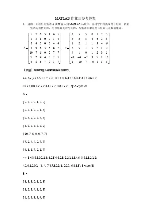
MA TLAB 作业三参考答案1、 请将下面给出的矩阵A 和B 输入到MA TLAB 环境中,并将它们转换成符号矩阵。
若某一矩阵为数值矩阵,另以矩阵为符号矩阵,两矩阵相乘是符号矩阵还是数值矩阵。
576516535501232310014325462564206441211346,39636623515212107600774101201724407734737812486721711076815A B ⎡⎤⎡⎤⎢⎥⎢⎥⎢⎥⎢⎥⎢⎥⎢⎥⎢⎥⎢⎥==⎢⎥⎢⎥⎢⎥⎢⎥⎢⎥⎢⎥---⎢⎥⎢⎥⎢⎥⎢⎥--⎣⎦⎣⎦【求解】矩阵的输入与转换是很直接的。
>> A=[5,7,6,5,1,6,5; 2,3,1,0,0,1,4; 6,4,2,0,6,4,4; 3,9,6,3,6,6,2; 10,7,6,0,0,7,7; 7,2,4,4,0,7,7; 4,8,6,7,2,1,7]; A=sym(A) A =[ 5, 7, 6, 5, 1, 6, 5] [ 2, 3, 1, 0, 0, 1, 4] [ 6, 4, 2, 0, 6, 4, 4] [ 3, 9, 6, 3, 6, 6, 2] [ 10, 7, 6, 0, 0, 7, 7] [ 7, 2, 4, 4, 0, 7, 7] [ 4, 8, 6, 7, 2, 1, 7]>> B=[3,5,5,0,1,2,3; 3,2,5,4,6,2,5; 1,2,1,1,3,4,6; 3,5,1,5,2,1,2; 4,1,0,1,2,0,1; -3,-4,-7,3,7,8,12; 1,-10,7,-6,8,1,5]; B=sym(B) B =[ 3, 5, 5, 0, 1, 2, 3] [ 3, 2, 5, 4, 6, 2, 5] [ 1, 2, 1, 1, 3, 4, 6] [ 3, 5, 1, 5, 2, 1, 2] [ 4, 1, 0, 1, 2, 0, 1][ -3, -4, -7, 3, 7, 8, 12] [ 1, -10, 7, -6, 8, 1, 5]2、 利用MA TLAB 语言提供的现成函数对习题1中给出的两个矩阵进行分析,判定它们是否为奇异矩阵,得出矩阵的秩、行列式、迹和逆矩阵,检验得出的逆矩阵是否正确。
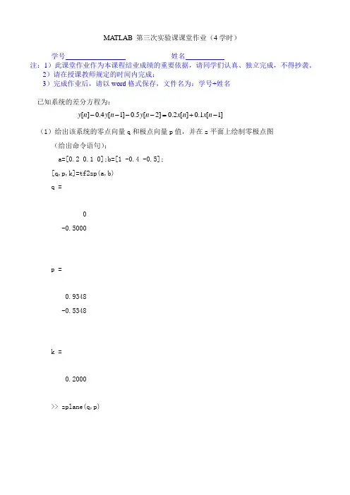
MATLAB 第三次实验课课堂作业(4学时)学号 姓名注:1)此课堂作业作为本课程结业成绩的重要依据,请同学们认真、独立完成,不得抄袭。
2)请在授课教师规定的时间内完成;3)完成作业后,请以word 格式保存,文件名为:学号+姓名已知系统的差分方程为:(1)给出该系统的零点向量q 和极点向量p 值,并在z 平面上绘制零极点图(给出命令语句);a=[0.2 0.1 0];b=[1 -0.4 -0.5];[q,p,k]=tf2zp(a,b)q =0 -0.5000 p =0.9348 -0.5348 k =0.2000>> zplane(q,p)[]0.4[1]0.5[2]0.2[]0.1[1]y n y n y n x n x n ----=+--1-0.500.51-1-0.8-0.6-0.4-0.200.20.40.60.81Real PartI m a g i n a r y P a r t(2)给出求该系统的单位冲激响应,并作出冲激响应的时域图(给出命令语句); a=[0.2 0.1 0];b=[1 -0.4 -0.5]; [h,t]=impz(a,b,7,1000) h =0.2000 0.1800 0.1720 0.1588 0.1495 0.1392 0.1304 t =0 0.0010 0.0020 0.0030 0.0040 0.0050 0.0060>> subplot(1,2,1);stem(t,h) >> subplot(1,2,2);impz(a,b)246x 10-3n (samples)A m p l i t u d e(3)绘制该系统的频响特性图(给出命令语句); >> num=[0.2 0.1 0] num =0.2000 0.1000 0>> den=[1 -0.4 -0.5] den =1.0000 -0.4000 -0.5000>> num=[0.2 0.1 0] num =0.2000 0.1000 0>> freqz(num,den)00.10.20.30.40.50.60.70.80.91-80-60-40-20Normalized Frequency (⨯π rad/sample)P h a s e (d e g r e e s )00.10.20.30.40.50.60.70.80.91-20-1010Normalized Frequency (⨯π rad/sample)M a g n i t u d e (d B )(4)试在Simulink 下绘制系统的结构图,并给出该系统的单位阶跃响应波形图。

m a t l a b综合大作业(附详细答案)-标准化文件发布号:(9456-EUATWK-MWUB-WUNN-INNUL-DDQTY-KII《MATLAB语言及应用》期末大作业报告1.数组的创建和访问(20分,每小题2分):1)利用randn函数生成均值为1,方差为4的5*5矩阵A;实验程序:A=1+sqrt(4)*randn(5)实验结果:A =0.1349 3.3818 0.6266 1.2279 1.5888-2.3312 3.3783 2.4516 3.1335 -1.67241.2507 0.9247 -0.1766 1.11862.42861.5754 1.6546 5.3664 0.8087 4.2471-1.2929 1.3493 0.7272 -0.6647 -0.38362)将矩阵A按列拉长得到矩阵B;实验程序:B=A(:)实验结果:B =0.1349-2.33121.25071.5754-1.29293.38183.37830.92471.65461.34930.62662.4516-0.17665.36640.72721.22793.13351.11860.8087-0.66471.5888-1.67242.42864.2471-0.38363)提取矩阵A的第2行、第3行、第2列和第4列元素组成2*2的矩阵C;实验程序:C=[A(2,2),A(2,4);A(3,2),A(3,4)]实验结果:C =3.3783 3.13350.9247 1.11864)寻找矩阵A中大于0的元素;]实验程序:G=A(find(A>0))实验结果:G =0.13491.25071.57543.38183.37830.92471.65461.34930.62662.45165.36640.72721.22793.13351.11860.80871.58882.42864.24715)求矩阵A的转置矩阵D;实验程序:D=A'实验结果:D =0.1349 -2.3312 1.2507 1.5754 -1.29293.3818 3.3783 0.9247 1.6546 1.34930.6266 2.4516 -0.1766 5.3664 0.72721.2279 3.1335 1.1186 0.8087 -0.66471.5888 -1.67242.4286 4.2471 -0.38366)对矩阵A进行上下对称交换后进行左右对称交换得到矩阵E;实验程序:E=flipud(fliplr(A))实验结果:E =-0.3836 -0.6647 0.7272 1.3493 -1.29294.2471 0.80875.3664 1.6546 1.57542.4286 1.1186 -0.1766 0.9247 1.2507-1.6724 3.1335 2.4516 3.3783 -2.33121.5888 1.2279 0.6266 3.3818 0.13497)删除矩阵A的第2列和第4列得到矩阵F;实验程序:F=A;F(:,[2,4])=[]实验结果:F =0.1349 0.6266 1.5888-2.3312 2.4516 -1.67241.2507 -0.17662.42861.5754 5.3664 4.2471-1.2929 0.7272 -0.38368)求矩阵A的特征值和特征向量;实验程序:[Av,Ad]=eig(A)实验结果:特征向量Av =-0.4777 0.1090 + 0.3829i 0.1090 - 0.3829i -0.7900 -0.2579 -0.5651 -0.5944 -0.5944 -0.3439 -0.1272-0.2862 0.2779 + 0.0196i 0.2779 - 0.0196i -0.0612 -0.5682 -0.6087 0.5042 - 0.2283i 0.5042 + 0.2283i 0.0343 0.6786 0.0080 -0.1028 + 0.3059i -0.1028 - 0.3059i 0.5026 0.3660 特征值Ad =6.0481 0 0 0 00 -0.2877 + 3.4850i 0 0 00 0 -0.2877 - 3.4850i 0 00 0 0 0.5915 00 0 0 0 -2.30249)求矩阵A的每一列的和值;实验程序:lieSUM=sum(A)实验结果:lieSUM =-0.6632 10.6888 8.9951 5.6240 6.208710)求矩阵A的每一列的平均值;实验程序:average=mean(A)实验结果:average =-0.1326 2.1378 1.7990 1.1248 1.24172.符号计算(10分,每小题5分):1)求方程组20,0++=++=关于,y z的解;uy vz w y z w实验程序:S = solve('u*y^2 + v*z+w=0', 'y+z+w=0','y,z');y= S. y, z=S. z实验结果:y =[ -1/2/u*(-2*u*w-v+(4*u*w*v+v^2-4*u*w)^(1/2))-w] [ -1/2/u*(-2*u*w-v-(4*u*w*v+v^2-4*u*w)^(1/2))-w] z =[ 1/2/u*(-2*u*w-v+(4*u*w*v+v^2-4*u*w)^(1/2))] [ 1/2/u*(-2*u*w-v-(4*u*w*v+v^2-4*u*w)^(1/2))]2)利用dsolve 求解偏微分方程,dx dyy x dt dt==-的解; 实验程序:[x,y]=dsolve('Dx=y','Dy=-x')实验结果:x =-C1*cos(t)+C2*sin(t)y = C1*sin(t)+C2*cos(t)3.数据和函数的可视化(20分,每小题5分):1)二维图形绘制:绘制方程2222125x y a a +=-表示的一组椭圆,其中0.5:0.5:4.5a =;实验程序:t=0:0.01*pi:2*pi; for a=0.5:0.5:4.5; x=a*cos(t); y=sqrt(25-a^2)*sin(t); plot(x,y) hold on end实验结果:2) 利用plotyy 指令在同一张图上绘制sin y x =和10x y =在[0,4]x ∈上的曲线;实验程序:x=0:0.1:4; y1=sin(x); y2=10.^x;[ax,h1,h2]=plotyy(x,y1,x,y2); set(h1,'LineStyle','.','color','r'); set(h2,'LineStyle','-','color','g'); legend([h1,h2],{'y=sinx';'y=10^x'});实验结果:3)用曲面图表示函数22z x y =+;实验程序:x=-3:0.1:3; y=-3:0.1:3; [X,Y]=meshgrid(x,y); Z=X.^2+Y.^2; surf(X,Y,Z)实验结果:4)用stem 函数绘制对函数cos 4y t π=的采样序列;实验程序:t=-8:0.1:8;y=cos(pi.*t/4); stem(y)实验结果:4. 设采样频率为Fs = 1000 Hz ,已知原始信号为)150π2sin(2)80π2sin(t t x ⨯+⨯=,由于某一原因,原始信号被白噪声污染,实际获得的信号为))((ˆt size randn x x+=,要求设计出一个FIR 滤波器恢复出原始信号。

Matlab Worksheet 1Part A1. Get into Matlab: Use the diary command to record your activity in to a file: diary mydiary01.doc before you start your work. (And diary off to switch off your diary when you finish your work.)At the Command Window assign a v alue x=10, then use the Up Key ↑ to repeat the expression, editing it to show the effect of using a semicolon after the 10, namely x=10;Answers:>> x=10x =10>> x=10;2. Confirm whether the following names of variables are acceptable: a) Velocity Yes Nob) Velocity1 Yes Noc) Velocity.1 Yes Nod) Velocity_1 Yes Noe) Velocity-01 Yes Nof) velocityONE Yes Nog) 1velocity Yes No3. Assign two scalar variables x and y values x=1.5, y=2.3, then construct Matlab expressions for the following: a) y x y x z +=35 b) ()3/27y x z = c) ()y e x x z 25106/111log -⋅⎥⎦⎤⎢⎣⎡+-= d) )2cos()2sin(x e y x z x ππ+-=Answers:>> x=1.5;y=2.3z1=5*x^3*y/(x+y)z2=(x^7*y^0.5)^(2/3)z3=(x^(1/6)/(log10(x^5-1))+1)*exp(-2*y)z4=sin(2*pi*x-y)+exp(x).*cos(2*pi*x)z1 =10.2138z2 =8.7566z3 =0.0232z4 =-3.73604. Assign two variables with complex values u=2+3j and v=4+10j and then construct expression for:a) v u b) j uv 2+ c) ju 2 d) u j ve π2- Answers:>> u=2+3j;v=4+10j;z1=u/vz2=u*v+2jz3=u/2jz4=v*exp(-j*2*pi*u)z1 =0.3276 - 0.0690iz2 =-22.0000 +34.0000iz3 =1.5000 - 1.0000iz4 =6.1421e+08 + 1.5355e+09ie the colon operator : to assign numerical values between 0 and 1 to vector arrayvariable a in steps of 0.1.Answer:>> V=0:0.1:1V =Columns 1 through 100 0.1000 0.2000 0.3000 0.4000 0.5000 0.6000 0.7000 0.80000.9000Column 111.0000e linspace function to assign 20 values to vector variable y between 20 and 30.Answer:>> V=linspace(20,30,20)V =Columns 1 through 1020.0000 20.5263 21.0526 21.5789 22.1053 22.6316 23.1579 23.684224.2105 24.7368Columns 11 through 2025.2632 25.7895 26.3158 26.8421 27.3684 27.8947 28.4211 28.947429.4737 30.00007.Assign 20 values to a variable h increasing logarithmically between 10 and 1000.Next, use the colon operator to assign the first 10 elements of h to a variable p.Answers:>> v=logspace(1,3,20)v =1.0e+03 *Columns 1 through 100.0100 0.0127 0.0162 0.0207 0.0264 0.0336 0.0428 0.05460.0695 0.0886Columns 11 through 200.1129 0.1438 0.1833 0.2336 0.2976 0.3793 0.4833 0.61580.7848 1.0000>> p=v(1:10)p =10.0000 12.7427 16.2378 20.6914 26.3665 33.5982 42.8133 54.5559 69.519388.58678.Create 6 element row vector z with values 1.0 1.2 1.6 -1.7 1.8 1.9, then constructan expression for the sum of the 2nd 4th and 6th elements of z.Answers:>> z=[1.0 1.2 1.6 -1.7 1.8 1.9]x=z(2)+z(4)+z(6)z =1.0000 1.2000 1.6000 -1.7000 1.8000 1.9000x =1.4000e the colon operator to create a vector array x between 10 and -10in steps of -1,and second, an array vector y between 20 and -20 in steps -2 .a)Add x and y, b) subtract 10x from 5y.Answers:>> x=10:-1:-10y=20:-2:-20x =Columns 1 through 1710 9 8 7 6 5 4 3 2 1 0 -1 -2 -3 -4 -5 -6Columns 18 through 21-7 -8 -9 -10y =Columns 1 through 1720 18 16 14 12 10 8 6 4 2 0 -2 -4 -6 -8 -10 -12Columns 18 through 21-14 -16 -18 -20>> x+yans =Columns 1 through 1730 27 24 21 18 15 12 9 6 3 0 -3 -6 -9 -12 -15 -18Columns 18 through 21-21 -24 -27 -30>> 5*y-10*xans =Columns 1 through 170 0 0 0 0 0 0 0 0 0 0 0 0 0 0 0 0Columns 18 through 210 0 0 0e the size,length, who and whos commands to establish the size and length of xand y from Question 9, and use transpose operator ’ to convert vector x fromQuestion 9.Answers:>> size(x)length(x)ans =1 21ans =21>> whoYour variables are:ans x y>> whosName Size Bytes Class Attributesans 1x1 8 doublex 1x21 168 doubley 1x21 168 double>> z=x'z =10987654321-1-2-3-4-5-6-7-8-9-1011.Show that if w=[ 2i 3i 3+i] the .’ operator creates the transpose. What effect does theoperator ’ applied to w have on its own?Answer:>> w=[ 2i 3i 3+i]w =0 + 2.0000i 0 + 3.0000i 3.0000 + 1.0000i>> x=w'x =0 - 2.0000i0 - 3.0000i3.0000 - 1.0000i>> y=w.'y =0 + 2.0000i0 + 3.0000i3.0000 + 1.0000ie the ones function to create a 4 by 6 array of 1’s. Considering just the shape ofthe resulting array, what do the expression ones(3), ones(5) and ones(7) all have in common?Answer:>> v=ones(4,6)v =1 1 1 1 1 11 1 1 1 1 11 1 1 1 1 11 1 1 1 1 1>> ones(3)ans =1 1 11 1 11 1 1>> ones(5)ans =1 1 1 1 11 1 1 1 11 1 1 1 11 1 1 1 11 1 1 1 1Ones(n)是n阶全为1的方阵13.Create using the rand function a 5 by 4 random matrix and assign it to matrix arrayvariable A and observe carefully what A(:,3) A(1:2) and A(3,[2 4]) mean.Answer:>> A=rand(5,4)A =0.8147 0.0975 0.1576 0.14190.9058 0.2785 0.9706 0.42180.1270 0.5469 0.9572 0.91570.9134 0.9575 0.4854 0.79220.6324 0.9649 0.8003 0.9595>> A(:,3)ans =0.15760.97060.95720.48540.8003>> A(1:2)ans =0.8147 0.9058>> A(3,[2 4])ans =0.5469 0.9157ing array subscripts, create an expression for the sum of the element in the topright-hand-corner of A and the bottom left-hand-corner of A. Also assign the 2nd column of A to a column vector b, and assign the 3rd row of A to a row vector d.Answer:>> A=rand(5,4)A =0.7513 0.9593 0.8407 0.35000.2551 0.5472 0.2543 0.19660.5060 0.1386 0.8143 0.25110.6991 0.1493 0.2435 0.61600.8909 0.2575 0.9293 0.4733>> x=A(1,4)+A(4,1)x =1.0491>> b=A(:,2)b =0.95930.54720.13860.14930.2575>> d=A(3,:)d =0.5060 0.1386 0.8143 0.2511>>diary off to switch off your diary now.15. Using the colon operator, assign a row vector array t, values between 0 and 10 in steps of 0.01. Use the ; operator to prevent displaying the information. Obtain the term-by-term values of functions:a) t e z 05.0-= b) )sin(05.0t e z t π-= c) )2cos()sin(05.0t t e z t ππ-=Answers:0.5874 0.6186 0.6473 0.6731 0.6958 0.7153 0.7314 0.7439 0.75280.7581Columns 551 through 5600.7596 0.7573 0.7513 0.7417 0.7284 0.7117 0.6916 0.6684 0.64210.6131Columns 561 through 5700.5815 0.5476 0.5117 0.4741 0.4350 0.3948 0.3538 0.3123 0.27060.2291Columns 571 through 5800.1880 0.1477 0.1085 0.0706 0.0344 0.0000 -0.0322 -0.0621-0.0895 -0.1141Columns 581 through 590-0.1359 -0.1548 -0.1705 -0.1832 -0.1928 -0.1992 -0.2025 -0.2027 - 0.2000 -0.1944Columns 591 through 600-0.1861 -0.1753 -0.1621 -0.1467 -0.1295 -0.1105 -0.0901 -0.0686 -0.0462 -0.0232Columns 601 through 610-0.0000 0.0232 0.0461 0.0684 0.0898 0.1099 0.1287 0.1457 0.1608 0.1737Columns 611 through 6200.1843 0.1923 0.1976 0.2001 0.1997 0.1962 0.1897 0.1801 0.1675 0.1518Columns 621 through 6300.1332 0.1117 0.0875 0.0607 0.0315 -0.0000 -0.0335 -0.0687 -0.1055 -0.1435Columns 631 through 640-0.1824 -0.2221 -0.2621 -0.3022 -0.3420 -0.3813 -0.4197 -0.4569 -0.4927 -0.5267Columns 641 through 650-0.5587 -0.5885 -0.6157 -0.6403 -0.6619 -0.6804 -0.6957 -0.7076 -0.7161 -0.7211Columns 651 through 660-0.7225 -0.7204 -0.7147 -0.7055 -0.6929 -0.6770 -0.6579 -0.6358 -0.6108 -0.5832Columns 661 through 670-0.5532 -0.5209 -0.4868 -0.4510 -0.4138 -0.3756 -0.3366 -0.2971 -0.2574 -0.2179Columns 671 through 680-0.1788 -0.1405 -0.1032 -0.0672 -0.0327 -0.0000 0.0307 0.05910.0851 0.1085Columns 681 through 6900.1293 0.1472 0.1622 0.1743 0.1834 0.1895 0.1926 0.1928 0.1902 0.1849Columns 691 through 7000.1771 0.1667 0.1542 0.1396 0.1231 0.1051 0.0857 0.0652 0.0439 0.0221Columns 701 through 7100.0000 -0.0221 -0.0439 -0.0650 -0.0854 -0.1046 -0.1224 -0.1386 - 0.1530 -0.1653Columns 711 through 720-0.1753 -0.1829 -0.1880 -0.1903 -0.1899 -0.1866 -0.1805 -0.1713 - 0.1593 -0.1444Columns 721 through 730-0.1267 -0.1063 -0.0832 -0.0577 -0.0299 0.0000 0.0318 0.06540.1003 0.1365Columns 731 through 7400.1735 0.2113 0.2493 0.2874 0.3253 0.3627 0.3992 0.4346 0.4686 0.5010Columns 741 through 7500.5315 0.5598 0.5857 0.6090 0.6296 0.6472 0.6618 0.6731 0.68120.6859Columns 751 through 7600.6873 0.6853 0.6798 0.6711 0.6591 0.6440 0.6258 0.6048 0.5810 0.5548Columns 761 through 7700.5262 0.4955 0.4630 0.4290 0.3936 0.3573 0.3201 0.2826 0.2449 0.2073Columns 771 through 7800.1701 0.1336 0.0981 0.0639 0.0311 0.0000-0.0292 -0.0562 -0.0809 -0.1033Columns 781 through 790-0.1230 -0.1400 -0.1543 -0.1658 -0.1744 -0.1802 -0.1832 -0.1834 -0.1810 -0.1759Columns 791 through 800-0.1684 -0.1586 -0.1467 -0.1328 -0.1171 -0.1000 -0.0815 -0.0621 -0.0418 -0.0210Columns 801 through 810-0.0000 0.0210 0.0417 0.0619 0.0812 0.0995 0.1164 0.1318 0.1455 0.1572Columns 811 through 8200.1667 0.1740 0.1788 0.1811 0.1807 0.1775 0.1717 0.1630 0.1516 0.1374Columns 821 through 8300.1205 0.1011 0.0792 0.0549 0.0285 0.0000 -0.0303 -0.0622 -0.0954 -0.1298Columns 831 through 840-0.1651 -0.2010 -0.2372 -0.2734 -0.3094 -0.3450 -0.3797 -0.4134 - 0.4458 -0.4766Columns 841 through 850-0.5055 -0.5325 -0.5571 -0.5793 -0.5989 -0.6157 -0.6295 -0.6403 - 0.6480 -0.6525Columns 851 through 860-0.6538 -0.6518 -0.6467 -0.6384 -0.6270 -0.6126 -0.5953 -0.5753 - 0.5527 -0.5277Columns 861 through 870-0.5005 -0.4714 -0.4405 -0.4081 -0.3744 -0.3398 -0.3045 -0.2688 - 0.2329 -0.1972Columns 871 through 880-0.1618 -0.1271 -0.0934 -0.0608 -0.0296 -0.0000 0.0277 0.05350.0770 0.0982Columns 881 through 8900.1170 0.1332 0.1468 0.1577 0.1659 0.1714 0.1743 0.1745 0.1721 0.1673Columns 891 through 9000.1602 0.1509 0.1395 0.1263 0.1114 0.0951 0.0776 0.0590 0.0398 0.0200Columns 901 through 9100.0000 -0.0200 -0.0397 -0.0589 -0.0773 -0.0946 -0.1108 -0.1254 - 0.1384 -0.1495Columns 911 through 920-0.1586 -0.1655 -0.1701 -0.1722 -0.1718 -0.1689 -0.1633 -0.1550 - 0.1442 -0.1307Columns 921 through 930-0.1147 -0.0962 -0.0753 -0.0522 -0.0271 -0.0000 0.0288 0.05910.0908 0.1235Columns 931 through 9400.1570 0.1912 0.2256 0.2601 0.2944 0.3281 0.3612 0.3932 0.4240 0.4533Columns 941 through 9500.4809 0.5065 0.5300 0.5511 0.5697 0.5856 0.5988 0.6091 0.6164 0.6207Columns 951 through 9600.6219 0.6200 0.6151 0.6072 0.5964 0.5827 0.5663 0.5472 0.5257 0.5020Columns 961 through 9700.4761 0.4484 0.4190 0.3882 0.3562 0.3233 0.2897 0.2557 0.2216 0.1876Columns 971 through 9800.1539 0.1209 0.0888 0.0578 0.0281 0.0000-0.0264 -0.0509 -0.0732 -0.0934Columns 981 through 990-0.1113 -0.1267 -0.1396 -0.1500 -0.1578 -0.1631 -0.1658 -0.1660 -0.1637 -0.1592Columns 991 through 1000-0.1524 -0.1435 -0.1327 -0.1201 -0.1060 -0.0905 -0.0738 -0.0562 -0.0378 -0.0190Column 1001-0.000016.For Question 15 c), use the plot function to plot the value z against t. And usexlabel and ylabel to label the t axis ‘time’ and z axis ‘Response’ and use title to give your figure a title. Copy the figure into your mydiary01.doc (from the figure edit menu, select copy, then open mydiary01.doc and paste in the figure as an object).Answers:>> plot(t,z3,'m','LineWidth',2)xlabel('time')ylabel('Response')title('z=exp(-0.05*t)*sin(πt)*cos(2πt))')Part B1.Create a new Script m-file, called myfirst.m, to assign values to three vector arraysa, b, and c; add each component together and assign to array d, whereA=[ 1, 2, 3], b=[4 5 6], c=[7 8 9]. Run myfirst.m. Examine the variable values in the WorkSpace . Edit myfirst.m to change variable b to b=[10 20 30]. Re-run myfirst.mAnswers:myfirst.mA=[ 1, 2, 3];B=[4 5 6];C=[7 8 9];D=A+B+Cresult:>> myfirstD =12 15 18myfirst.mA=[ 1, 2, 3];B=[10 20 30];C=[7 8 9];D=A+B+C(2-2)result:>> myfirstD =18 30 422.Create a function m-file, called myfun.m, that accepts two arrays x and y asarguments, and produces the sum of x and y, and gives as the function output, the maximum of x+y.Answer:(1)myfun.mfunction[M] = myfun(x,y)%MAXIMUMsum=x+y;t=length(x)-1;fori=1:t;ifsum(1+i)>sum(i)max=sum(1+i);sum(1+i)=sum(i);endendM=maxend(2)result>> x=[1 2 3]y=[4 5 6]x =1 2 3y =4 5 6>> myfun(x,y)M =9ans =93.Modify your script m-file myfirst.m by calling in it myfun.m twice, namely with aand b as parameters in the argument list, and second with parameters b and c. Run myfirst.mand afterwards. Examine the WorkSpace variable values.Answers:(1)myfirst_modify.mA=[ 1, 2, 3];B=[10 20 30];myfun(A,B);disp('calling myfun again')C=[7 8 9];myfun(B,C);(2)result>> myfirst_modifyM =33calling myfun againM =394. Modify your script m-file myfirst.m by introducing variables A and B. Assignscalar values A=1, B=2. Declare A and B as global variables both in myfirst.m and myfun.m. Modify myfun.m by adding A and B to the maximum value of x+y. Answers:(1)myfirst.mglobalA B;A=1;a=[ 1, 2, 3];b=[10 20 30];myfun(a,b);disp('calling myfun again')c=[7 8 9];d=a+b+c;;myfun(c,d);(2)myfun.mfunction[M] = myfun(x,y)%MAXIMUMglobalA B;A=1;B=2;sum=x+y;t=length(x)-1;fori=1:t;ifsum(1+i)>sum(i)max=sum(1+i);sum(1+i)=sum(i);endM=max+A+Bend(3)result>> myfirstM =36calling myfun againM =545.Create a script m-file and, using a pair of nested for loops, assign to a 5 by 5matrix array A, values equal to the sum of the subscripts. Ensure that the array is first cleared before the loops and afterwards display the array values. Run the m-file.Answer:(1)home_work_1_B_5.mclearall;closeall;fori=1:5forj=1:5A(i,j)=i+j;endendA(2)result>> home_work_1_B_5A =2 3 4 5 63 4 5 6 74 5 6 7 85 6 7 8 96 7 8 9 106. Relational Operators:- Assign variables x=1 and y=2, then examine the values of the expressions:a) x>y, b)x<y, c) x==y. What is the value of z=(x>y)*(x==y)?Answer:(1)home_work_1_B_6.mx=1;y=2;u1=x>yu2=x<yu3=(x==y)z=(x>y)*(x==y)(2)result>> home_work_1_B_6u1 =u2 =1u3 =z =7. While loop:- Create a script m-file, and using a ‘while loop’, generate the partial sum for the series: ...31211+++πππ which stops adding-on terms when they are less than 1e-6 times the total sum.Answer:(1)home_wor_1_B_7.mclear all;close all;i=1;sum=0;t=1/pi;whilet>=exp(-6)sum=sum+t;i=i+1;t=1/(i*pi);enddisp('多项式之和sum') sumdisp('循环次数i')idisp('多项式最后一项t') t(2)result>> >> home_work_1_B_7 多项式之和sumsum =1.7294循环次数ii =129多项式最后一项tt =0.00258. While loop:- Use a ‘while loop’ to keep adding array A to itself until just one ofthe elements in A is greater than, but not equal to 40 where, initially ⎥⎦⎤⎢⎣⎡=4321A .Answer:(1)home_work_1_B_8.mA=[1 2 3 4 ];m=max(A(:));whilem<=40;A=A+A;m=max(A(:));endA(2)result>> home_work_1_B_8A =16 3248 649. If statements:- Create a function m-file that receives variable x and y as arguments, then uses an ‘if’ statement internally to execute the condition that: ‘if x is greater than y the function takes the value x, otherwise it takes the value y’. Test it on 2 numbers x=1 and y=1.Answer(1)greater.mfunction[ max ] = greater( x,y )%lbs_home_work_1_B_9ifx>y max=x;elsemax=y;endend(1) result>> x=1;y=1;>> greater(x,y)ans =110.If statements:- Create a function m-file that receives variable x, y and z asarguments, then uses an ‘if elseif and else’ statements, generate the output value to be =x if first of all x>1, otherwise =y if y>10, otherwise =z if z>20, otherwise =1 if none of those conditions hold. Test it on values (100,100,100) and (0, 0,0).Answer:(1)compare.mfunction[max] = compare( x,y,z )%lbs_home_work_1_B_10ifx>1 max=x;elseify>10 max=y;elseifz>2 max=z;elsemax=1;endendendmaxend(2)result>> compare(100,100,100)max =100ans =100>> compare(0,0,0)max =1ans =111.Switch Statement:- Create a function with one input argument x to test whether theexpression: real(x^2) is equal to 0,1, or -1, which then displays a string stating appropriately whether: ‘x is equal to zero’, ‘x is equal to +1 or -1’ or ‘x is equal to +j or –j’; otherwise display ‘test failed’. Test your m-file on three values: x=0, x=10 and x=j (1j).-=(1)test.mfunctionf = test( x%lbs home work 1 partB 11t=real(x^2);Switch tcase 0, disp('x is equal to zero');case1, disp('x is equal to +1');case-1, disp('x is equal to -1');otherwisedisp('test failed');end(2) result>> test(10)test failed>> test(0)x is equal to zero>> test(j)x is equal to -112. Polynomials:- Create a script m-file to generate the 5th degree polynomial:104322345+++++x x x x x and find all the roots. Use the plot function to plot the polynomial between x=-2 and x=2. Give the plot a title ‘A 5th degree polynomial for different domains’.Answer:(1)home_work_1_B_12.mclear all;close all;x=-2:2;y=x.^5+2*x.^4+3*x.^3+4*x.^2+x+10plot(x,y,'m','LineWidth',2)axis([-2 2 -2 120])p=[1 2 3 4 1 10]roots(p)(2)result:home_work_1_B_12y =0 11 10 21 116p =1 2 3 4 1 10-2.0000-0.6566 + 1.6409i-0.6566 - 1.6409i0.6566 + 1.0815i0.6566 - 1.0815i(3)home_work_1_B_12.fig。
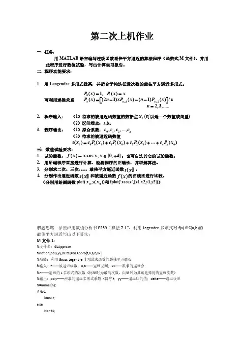
第二次上机作业一. 任务: 用MATLAB 语言编写连续函数最佳平方逼近的算法程序(函数式M 文件)。
并用此程序进行数值试验,写出计算实习报告。
二. 程序功能要求:1.用Lengendre 多项式做基,并适合于构造任意次数的最佳平方逼近多项式。
可利用递推关系0112()1,()()(21)()(1)()/2,3,.....n n n P x P x x P x n xP x n P x nn --===---⎡⎤⎣⎦=2.程序输入:(1)待求的被逼近函数值的数据点(可以是一个数值或向量)0x (2)区间端点:a,b 。
3. 程序输出:(1)拟合系数:012,,,...,nc c c c (2)待求的被逼近函数值00001102200()()()()()n n s x c P x c P x c P x c P x =++++ 三:数值试验要求:1.试验函数:;也可自选其它的试验函数。
()cos ,[0,4]f x x x x =∈+2.用所编程序直接进行计算,检测程序的正确性,并理解算法。
3.分别求二次、三次、。
最佳平方逼近函数。
)x s (4.分别作出逼近函数和被逼近函数的曲线图进行比较。
)x s ()(x f (分别用绘图函数plot(,s())和fplot(‘x cos x ’,[x 1 x 2,y 1,y 2]))0x 0x 解题思路:参照应用数值分析书P259“算法7-1”,利用Legendre 多项式对f(x)∈C(a,b)的最佳平方逼近写出以下算法:M 文件1:%文件名:GLAppro.mfunction[poly,yy,delta]=GLAppro(f,n,a,b,xx)%功能:利用Gauss Legendre 多项式求函数的最佳平方逼近%输入:f ——被逼近函数;a,b ——逼近区间;xx ——欲求的逼近点%n ——逼近的L 多项式的次数(标量时为最高次数,向量时为其所选择的的逼近次数)%输出:poly ——所求的逼近多项式系数(降序);yy ——逼近店的值;delta ——逼近误差N=numel(n);if N>1id=n+1;elseN=n+1;enddelta=quad(@myfun,-1,1,[],[],f,a,b);c=zeros(1,N);poly=zeros(1,id(N)); for k=1:Nc(k)=(2*id(k)-1)*quad(@fLegPoly,-1,1,[],[],f,id(k)-1,a,b)/2;delta=delta-c(k)^2*2/(2*id(k)-1);endif nargin==5t0=(2*xx-a-b)/(b-a);yy=zeros(size(xx));for k=1:Np=LegPoly(id(k)-1);yy=yy+c(k)*polyval(p,t0);poly(id(N)-id(k)+1:(id(N)))=poly(id(N)-id(k)+1:(id(N)))+c(k)*p;endelsefor k=1:Np=LegPoly(k-1);poly(N-k+1:N)=poly(N-k+1:N)+c(k)*p;endendM文件2:function y=myfun(t,f,a,b)%功能:GLAppro子函数,变换到区间[-1,1]x=(b-a)*t/2+(b+a)/2;y=f(x).*f(x);M文件3:function f=fLegPoly(t,f1,n,a,b)%功能:GLAppro子函数,求变换后的积分函数p=LegPoly(n);x=(b-a)*t/2+(b+a)/2;f=f1(x).*polyval(p,t);M文件4:function p=LegPoly(n)%功能:递归法求n次Gauss Legendre多项式%输入:n——多项式次数%输出:p——降幂排列的多项式系数p0=1;p1=[1,0];if n==0p=p0;elseif n==1p=p1;elsep=((2*n-1)*[LegPoly(n-1),0]-(n-1)*[0,0,LegPoly(n-2)])/n;end%文件名:homework2.mf=@(x)(x.*cos(x));n=cell(3,1);n{1}=2;n{2}=3;n{3}=4;a=0;b=4;x0=linspace(a,b)';color=['k','g','b'];y=f(x0);plot(x0,y,'r-','linewidth',1.5);hold on;syms t x;for i=1:3[poly,py,delta]=GLAppro(f,n{i},a,b,x0);pt=vpa(poly2sym(poly,t),4);poly=simple(subs(pt,t,(2*x-a-b)/(b-a)));poly=vpa(poly,4);disp(['所求的最佳评分那个逼近多项式为(n=' int2str(n{i}) '):']);disp(poly);disp(['误差为:' num2str(delta)]);plot(x0,py,color(i),'linewidth',1.5)end分别求两次、三次和四次最佳平方逼近函数s(x)输入:homework2输出:所求的最佳评分那个逼近多项式为(n=2):- 0.1599*x^2 - 0.572*x + 0.8268误差为:0.45032所求的最佳评分那个逼近多项式为(n=3):0.3818*x^3 - 2.45*x^2 + 3.093*x - 0.3948误差为:0.02393所求的最佳评分那个逼近多项式为(n=4):0.08539*x^4 - 0.3014*x^3 - 0.6939*x^2 + 1.531*x - 0.08255误差为:0.002258调整图象并标注:yx第三次上机作业一. 任务一:用MATLAB 语言编写化工原理流体力学中d-u-Re-λ试差法的算法程序(函数式M 文件)。
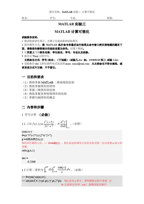
MATLAB 实验三MATLAB 计算可视化试验报告说明:1 做试验前请先预习,并独立完成试验和试验报告。
2 报告解答方式:将MATLAB 执行命令和最后运行结果从命令窗口拷贝到每题的题目下面,请将报告解答部分的底纹设置为灰色,以便于批阅。
3 在页眉上写清报告名称,学生姓名,学号,专业以及班级。
3 报告以Word 文档书写。
文档命名方式: 学号+姓名+_(下划线)+试验几.doc 如:110400220张三_试验1.doc 4 试验报告doc 文档以附件形式发送到maya_email@ 。
凡文档命名不符合规范,或者发送方式不正确,不予登记。
一 目的和要求(1)熟练掌握MATLAB 二维曲线的绘制(2)熟练掌握图形的修饰(3)掌握三维图形的绘制(4)熟练掌握各种特殊图形的绘制(5)掌握句柄图形的概念二 内容和步骤1 符号计算 (必做)1.1 已知725),(23+-=x y y x y x f ,求12=x dxdy f d 。
(必做) syms x yf=(x^3*y-5*y)/(2*x^2+7)g =diff(diff(f,x),y)%有同学调用方式:>> f1=diff(f,2) ,要注意这种调用方法其实是对第一自由变量x 求2阶导数。
subs(g,x,1)ans =0.53091.2计算二重积分⎰⎰-ππππy dx x x dy )sin(2。
(必做) >> f=sym('sin(x)/x');>> int(int(f,'x','y-pi',pi),'y',pi,2*pi) %注意对y 积分,要明确指定积分变量‘y ’ % 注意积分区间(a,b ),参数的前后顺序ans =21.3解方程组:221,2x y xy +== 。
(必做) >> S=solve('x^2+y^2=1','x*y=2',’x ’,’y ’);>> xx=double(S.x),yy=double(S.y)xx =1.1180 - 0.8660i1.1180 + 0.8660i-1.1180 - 0.8660i-1.1180 + 0.8660iyy =1.1180 + 0.8660i1.1180 - 0.8660i-1.1180 + 0.8660i-1.1180 - 0.8660i1.4 求微分方程022=+'+''y y y ,当0)0(=y ,1)0(='y 时的解。
matlab 期末大作业(30分,每题6分)1. 积分运算(第四数值和五章符号)(1)定积分运算:分别采用数值法(quad ,dblquad )和符号运算(syms, int )一重定积分π⎰1. 数值法(quad )a) 运行代码:b) 运行结果:2. 符号运算(syms )a) 运行代码:b) 运行结果:二重定积分112200()x y dxdy+⎰⎰1.数值法(dblquad):a)运行代码:b)运行结果:2.符号运算(syms):a)运行代码:b)运行结果:(2) 不定积分运算sin dxdy ⎰⎰((x/a)+b/y) i.运行代码:ii.运行结果:2. 用符号法和数值法求解线性代数方程 (第五章和第二章)⎩⎨⎧=+=+12*22x *213*12x *a11y a a y a (1) 用syms 定义待解符号变量x,y 和符号参数a11,a12,a21,a22,用符号solve 求x,y 通解 1. 运行代码:2. 运行结果:(2) 用subs 带入a11=2,a12=4,a21=6,a22=8,求x 和y 特解,用vpa 输出有效数值4位的结果 1. 运行代码:2. 运行结果:(3) 采用左除(\)和逆乘法求解符号参数赋值后的方程 ⎩⎨⎧=+=+12*8x *63*4x *2y y1. 运行代码:2. 运行结果:3.数值法和符号法求解非线性方程组(第四数值和五章符号 )(1)采用数值法(fsolve )求解初始估计值为x0 = [-5; -5]的数值解1. 运行代码:2. 运行结果:21x 21x 21e x 2x e x x 2--=+-=-(2)符号法(solve )的符号结果用eval 或double 转化为数值结果.1. 运行代码:2. 运行结果:4. 解二阶微分方程 (第四数值和五章符号 )⎪⎩⎪⎨⎧===++6)0(',0)0(09322y y y dx dy dx y d(1)数值ode 求特解,用plot (x,y) 画t 在[0,10]范围内(x ,y )数值曲线 1. 运行代码:2. 运行结果:(2)符号运算dsolve求通解,用ezplot画t在[0,10]范围内(x,y)符号曲线1. 运行代码:2. 运行结果:5. 三维绘图(第六章)已知:x和y都在[-8,8]范围内,采用subplot(3,1,x)绘制三个子图,它们分别是用meshgrid和mesh绘制网格图、用c=contour 绘制等位线和用surf 绘制曲面图1.运行代码:2.运行结果:。
《数学实验》报告实验名称 matlab的二维和三维曲线绘制学院材料科学与工程专业班级材料1009姓名周少坤学号 41030264日期 2012年4月30日一、【实验目的】1、学会并练习matlab二维和三维曲线绘图操作。
2、熟练掌握二维和三维绘图的图形标注。
3、掌握多个子窗口的图形绘制。
4、练习图形的阅读、调制。
二、【实验任务】1、练习79页1、3、5题。
三、【实验程序】&【实验结果】1/79:⑴:程序:结果:024********程序:结果:012345678910程序:结果:-202-202y=xcosxX 轴Y 轴4681012-101y=xtan(1/x)sin(x 3)X 轴Y 轴12345678910-2y=exp(1/x)sin(x)X 轴Y 轴5/79: 程序:结果:-100100X 轴Y 轴Z 轴四、【实验总结】通过本次实验,学会了matlab二维和三维的曲线绘制,熟练掌握了对所绘曲线的图名标注、图例标注、坐标轴标注以及多个子窗口的绘图等操作。
在多次练习的基础上,也加速了在命令窗口的命令输入操作,提高了绘图的一次成功率。
并在实验中出现只会出一个点和函数输入后总提示维数错误等问题,使我深刻认识到了命令窗口中分号与冒号的混淆,以及点乘与星乘的区别。
同时也掌握了在绘图窗口中对图形、图例等的调节,以及多方位、多视角的对图形进行阅读。
《MATLAB及应用》上机作业学院名称:机械工程学院专业班级:测控1201学生姓名:学生学号:201 年 4 月《MATLAB及应用》上机作业要求及规范一、作业提交方式:word文档打印后提交。
二、作业要求:1.封面:按要求填写学院、班级、姓名、学号,不要改变封面原有字体及大小。
2.内容:只需解答过程(结果为图形输出的可加上图形输出结果),不需原题目;为便于批阅,题与题之间应空出一行;每题答案只需直接将调试正确后的M文件内容复制到word 中(不要更改字体及大小),如下所示:%作业1_1clcA=[1 2 3 4;2 3 5 7;1 3 5 7;3 2 3 9;1 8 9 4];B=[1+4*i 4 3 6 7 7;2 3 3 5 5 4+2*i;2 6+7*i 5 3 4 2;1 8 9 5 4 3];C=A*BD=C(4:5,4:6)三、大作业评分标准:1.提交的打印文档是否符合要求;2.作业题的解答过程是否完整和正确;3.答辩过程中阐述是否清楚,问题是否回答正确;4.作业应独立完成,严禁直接拷贝别人的电子文档,发现雷同者都以无成绩论处。
作业11、用MATLAB 可以识别的格式输入下面两个矩阵12342357135732391894A ⎛⎫⎪⎪ ⎪= ⎪⎪ ⎪⎝⎭,144367723355422675342189543i i B i +⎛⎫⎪+⎪= ⎪+ ⎪⎪⎝⎭再求出它们的乘积矩阵C ,并将C 矩阵的右下角23⨯子矩阵赋给D 矩阵。
赋值完成后,调用相应的命令查看MATLAB 工作空间的占有情况。
解:A=[1 2 3 4;2 3 5 7;1 3 5 7 ;3 2 3 9 ;1 8 9 4;]B=[1+4i 4 3 6 7 7;2 3 3 5 5 4+2i;2 6+7i 5 3 4 2;1 8 9 5 4 3;] B=[1+4i 4 3 6 7 7;2 3 3 5 5 4+2i;2 6+7i 5 3 4 2;1 8 9 5 4 3;] C=A*B D=C(4:5,4:6);2、设矩阵16231351110897612414152⎛⎫⎪⎪ ⎪ ⎪⎝⎭,求A ,1A -,3A ,12A A -+,1'3A A --,并求矩阵A 的特征值和特征向量。
Matlab Worksheet 3Part A1. Using function conv_m.m to make convolution between the following to functions (x and h):x=[3, 11, 7, 0, -1, 7, -5, 0, 2]; h=[11, 9, 0, -7, -3, 2, 0 -1]; nx=[-2:6]; nh=[0:7];Plot the functions and convolution results.x=[3, 11, 7, 0, -1, 7,5,0, 2]; nx=[-2:6];h=[11, 9, 0, -7, -3,2,0,-1]; nh=[0:7];[y, ny]=conv_m(x,nx,h,nh); subplot(3,1,1); stem(nx,x); ylabel('x[n]');axis([-6 10 -20 20]); subplot(3,1,2); stem(nh,h); ylabel('h[n]');axis([-4 10 -20 20]); subplot(3,1,3); stem(ny,y); xlabel('n'); ylabel('y[n]');axis([-6 15 -200 200]);2. Plot the frequency response over π≤Ω≤0for the following transfer function by lettingΩ=j e z , where Ωis the frequency (rad/sample)., with appropriate labels and title.9.06.1)(2++=z z zz H .delta=0.01;Omega=0:delta:pi;H= (exp(j .* Omega)) ./ ((exp(j .* Omega)).^2+1.6*exp(j .* Omega)+0.9); subplot(2,1,1);plot(Omega, abs(H)); xlabel('0<\Omega<\pi'); ylabel('|H(\Omega)|');axis([0 pi 0 max(abs(H))]); subplot(2,1,2);plot(Omega,atan2(imag(H),real(H))); xlabel('0<\Omega<\pi');ylabel(' -\pi < \Phi_H <\pi') axis([0 pi -pi pi]);3. Use fft to analyse following signal by plotting the original signal and its spectrum.⎪⎭⎫ ⎝⎛+⎪⎭⎫ ⎝⎛+⎪⎭⎫ ⎝⎛=10244672sin 10241372sin 1024322sin ][n n n n x πππ.% fft N=1024; dt=1/N;t=0:dt:1-dt;x=sin(2*pi*32 .*t) +sin(2*pi*137 .*t)+sin(2*pi*467 .*t) ; subplot(2,1,1);plot(t,x), xlabel('t sec'),ylabel('x'); title('Signal and its Fourier Transform'); axis([min(t) max(t) 1.5*min(x) 1.5*max(x)]); X=fft(x); f=0:N-1;subplot(2,1,2);stem(f,abs(X)), xlabel('Hz'), ylabel('|X|'); axis([ 0 N/2 0 1.5*max(abs(X))]);4. Use the fast Fourier transform function fft to analyse following signal. Plot the original signal,and the magnitude of its spectrum linearly and logarithmically. Apply Hamming window to reduce the leakage.⎪⎭⎫ ⎝⎛+⎪⎭⎫ ⎝⎛+⎪⎭⎫ ⎝⎛=10247.4672sin 10244.1372sin 10245.322sin ][n n n n x πππ.The hamming window can be coded in Matlab asfor n=1:Nhamming(n)=0.54+0.46*cos((2*n-N+1)*pi/N); end;where N is the data length in the FFT.%Examine signal components %sampling rate 1024Hz N=1024; dt=1/N;t=0:dt:1-dt;%****define the signal**x=0.1*sin(2*pi*32.5 .*t ) + ... 0.2*sin(2*pi*137.4 .*t )+ ... 0.15*sin(2*pi* 467.7 .*t ) ; %*********************** subplot(3,1,1); plot(t,x);axis([0 1 -1 1]);xlabel('nT (seconds)'); ylabel('x[n]');%hamming window for n=1:Nw(n)=0.54+0.46*cos((2*n-N+1)*pi/N); end ;x1=x .*w;subplot(3,1,2); plot(t,x1);axis([0 1 -5 5]);xlabel('nT (seconds)'); ylabel('x[n] Hamming win'); X=fft(x1);df=1;f=0:df:N-1;subplot(3,1,3);plot(f,20*log10(abs(X))); axis([0 N/2 -60 60]);xlabel('k (Hz)');ylabel('|X[k]| (db)');Part BSimulation Using SIMULINKINTRODUCTIONThe objective of this laboratory is to learn about various properties of signals and systems by doing simulations in SIMULINK.PART 1. BASICS OF SIMULINK1.1 UNDERSTANDING SIMPLE WAVEFORMS AND INTEGRATIONCreate a pulse of height 2 units from time 0 to 4 seconds by subtracting two unit steps and adding a gain. Connect this pulse to an integrator with a gain of 0.5 and a zero initial condition. Connect oscilloscopes to show the pulse and the output of the integrator. You may wish to name your simulation (block) diagram; to do so use the save as feature under edit. Your block diagram should be similar as below.Before simulating you need to pull down the simulation header and double click on parameters. Unless told otherwise always assume that you can use the ode 45 integration algorithm shown in this window and the other default parameters. Typically you will only alter the start and stop times but for this first simulation you can use the default values of 0 and 10 seconds. Double click on the oscilloscopes to get the windows in which the traces will appear, pull down the simulate menu and click on run. Plot below the integrator input and output waveforms.Repeat the experiment but with an initial condition of –2 on the integrator. Again draw the results.Repeat the experiment but with an initial condition of –2 on the integrator. Again draw the results.1.2 FIRST ORDER SYSTEMA single time constant may be simulated using the transfer function block in which you enter the coefficients of the numerator and denominator polynomials. Set up the configuration in a new SIMULINK window to realise the transfer function 1/(s+2) with the input unit step and an oscilloscope connected to the output of the transfer function block. Plot the block diagram in the space below. Simulate the system for 5 seconds and plot the response.1.3 SECOND ORDER SYSTEMFor the second order all pole transfer function )2/(200220ωωζω++s s you will recall that if a time scale of ω0t is used for plotting the step response, the response shape will only be affected by changes in the damping ratio ζ. This can also be shown if we normalise the transfer function by replacing (s/ω0) by s n togive )12/(12++n n s s ζ. To study the effect of varying ζ on the step response we will therefore use the transfer function 1/(s 2+2ζs+1). Set up the following configuration for a simulation study.i) A unit step input. ii) Connect the unit step to a transfer function of 1/(s 2+2ζs+1) with ζ = 1.0. iii) Take a summing block and connect the input step to a +ve input and the transfer functionoutput to a –ve input.iv) Connect the output of this summer to a square function. This is obtained by using f(u) in thenonlinear blocks.v)Connect the output of this squarer to an integrator.vi)Connect two oscilloscopes to the circuit, one to the transfer function output and the other to the output of the integrator.vii)Also connect simout blocks to the same signals as the oscilloscopes. Rename the one connected to the integrator output simout1.Simulate the system with the values of ζ listed in the table below and fill in the other figures from the simulation results. To get an accurate value at the end of each run you can type simout1 in the MATLAB window. You can also measure the overshoot by making use of the maximum command: simply type max(simout) in the MATLAB window.% overshoot 2.1076 1.2500 1.1778 1.0571 1.0000 1.1285 2.1431PART 2. SIMULATION OF AIRCRAFT PITCH ANGLE AND ALTITUTEThe purpose IS to use "SIMULINK" to simulate a (much simplified) model of the longitudinal motion of a fighter aircraft.The "angle of attack", is the angle between the direction a plane is pointing, and the direction in which it actually moves through the air. For a plane flying at approximately constant altitude, this is equivalent to the "pitch angle", φ, as illustrated in Fig.2.1. This angle is important because it produces a lift force perpendicular to the axis of the plane, and hence a "normal acceleration", a n , (also shown in the figure).vThe pilot wants to be able to control the pitch angle (倾斜角度), and does so ultimately by rotating the front fins, and tail elevators of the aircraft, shown in Fig. 2.2. The first task is therefore to model theeffect of these movements on the "pitch rate" q ()=φ, and "normal acceleration" a n .Fig. 2.2 Illustration of control surfaces2.1: MODELLING THE AIRCRAFT AND ACTUATOR DYNAMICSi) Normal Acceleration, a nThe acceleration of the aircraft in a direction perpendicular to its axis, (the "normal accel.", a n ), is determined mainly by the angle θ1 of the tail elevators of the aircraft shown in Fig. 2.2. Indeed aerodynamic modelling shows that this relationship can be described by the differential equation,11116342.364.1982.81.3θθθ++=-+ n n n a a aConvert this relationship into a transfer function form:-ii) Pitch Rate, qThe rate at which the pitch angle changes, (the "pitch rate", q ), is determined mainly by the angle θ2 of the front fins of the aircraft shown in Fig. 2.2. Indeed aerodynamic modelling shows that this relationship can be described by the differential equation,2227.1125.782.81.3θθ++=-+ q q qConvert this relationship into a transfer function form:-iii) Actuator Dynamics + GearsThe tail elevators of the aircraft are driven directly by a hydraulic actuator which has a transfer function,G s s ()()=-+1414/ (3)To a unit step input U(s)=1/s , the response R(s) = G(s)⋅U(s)= 1411)14(14++-=+-s s s s . What form ofstep response r(t) would you expect from this actuator, and what is its time constant?The front fins and the tail elevators are both driven from the actuator by the same drive shaft through a gear box. The same gear on this drive shaft connects to the tail elevator gear wheel, which has 500 teeth, and the front fin gear wheel, which has 100 teeth, the relationship between θ1 and θ2 is52112==t t θθ(4) 2.2: SIMULATING THE AIRCRAFT AND ACTUATOR DYNAMICSi) F or the aircraft model you will need from the Continuous or Maths Library:-∙a Transfer Fcn block to represent the "tail elevator angle → normal accel" relationship (eqn (1))∙ a Transfer Fcn block to represent "front fin angle → pitch rate" relationship, (see eqn (2)) ∙ a Transfer Fcn block to represent the hydraulic "actuator dynamics", (see eqn (3)) ∙ a Gain block to represent the "gears", (see eqn (4))from the Sources Library:-∙ a Step Input block to act as a test input - (set Step time = 5sec, and Final value = 0.01 rad)from the Sinks Library:- ∙a ‘Scope block to monitor the pitch rate output - (set Horizontal Range = 20sec).ii) Now connect the blocks together, using the step input to drive the actuator, and the actuator to drive the tail elevators. The actuator is also used to drive the front fins via the gearbox. The 'Scope should be connected to the output of the "front fin angle → pitch rate" block. Note: you can take a branch from a signal line by dragging with the right mouse button from the point on the line at which you want the branch to start.Plot the block diagram you have created in the box below:-iii) From the pull-down menus of your simulation window, select Simulation/Parameters , in order to define how the simulation is to be performed. Set:-Stop Time = 20 sec; Initial Step Size = 0.001; Max Step Size = 0.01;iv) Finally double click on your ‘scope, so that you can watch the progress of the simulation, and then select Simulation/Start from the pull-down menu of your simulation window. You may want to adjustthe Vertical Range of your 'Scope, and re-run the simulation to get a good picture. Plot the response of the aircraft pitch rate below, and comment on these results. Note that it can be shown that if a transfer function has a denominator polynomial with a zero or negative coefficient then it must have a root with a zero or positive real part.2.3: SIMULATING THE PITCH RATE CONTROL SYSTEMThe designers are quite glad they simulated the response of the aircraft, before trying it for real. They now decide to improve the response by measuring the output (ie. what is actually happening to the pitch rate), and subtracting this from the input (ie. what they would like to happen), to produce an error signal. The error signal will be amplified, and then used to drive the actuator (see Fig. 2.3). In this way the actuator will automatically act so as to reduce any differences between the input demand, and the output response.Fig. 2.3 Feedback control of pitch ratei) Before you simulate the control system described above, you will probably find that you are short of space in your simulation window. Besides it would be nice to package the aircraft + actuator dynamics as a single block, so that they are distinct from anything added later as shown in Fig. 2.3.If you press the left mouse button in an empty space of the window, you get a "rubber band" box which you can drag to surround a group of elements. When you release the button, all elements inside are "selected". Use this technique to select all the aircraft + actuator dynamics, (but leave out the step input and ‘scope monitor). From the pull-down menu under Edit select Create a Subsystem, and your diagram will suddenly look as shown in Fig. 2.4.Fig. 2.4 New diagramii) Rename the "Subsystem" as "Actuator + Aircraft Dynamics" as shown in Fig. 2.3 by editing the text below the block. You can see what is inside by double clicking on the block itself, - try it! Notice that the input and output connections are labelled "in_1", "out_1" etc. Edit these to give them more meaningful names.iii) Now construct the planned control system, as illustrated in Fig. 2.3. Notice the pilot is now represented by a Signal Generator (from the Sources library), which should be set to produce a Square Wave, of frequency 0.1 Hz and peak amplitude 0.5.iv) The designers are unsure what value to use for the Gain. Open the Pitch Rate 'Scope, and run the simulation first for the Gain = -0.5 (as shown above), and then for the Gain = -5. Plot the two responses you obtain, and comment on the relative advantages and disadvantages of each:-Comments on responses (in terms of overshot and response time etc):PART 3: SIMILATION OF NONLINEAR SHIP ROLL DYNAMICSThe rolling motion of ships is of considerable interest to naval architects because even today around 50% of ships lost at sea, sink as a result of a capsize. The aim of this laboratory is to study such behaviour by:-∙constructing a nonlinear differential equation model for the system∙converting this model into a phase variable block diagram form suitable for simulation∙simulating the (nonlinear) response to sinusoidal excitation∙calculating the steady state response for a ship whose cargo has shifted dangerously to one sideFig. 3.1 Ship schematic3.1: MODELLING AND SIMULATION OF SHIP DYNAMICSi) Consider the ship sketch shown in Fig. 3.1. Given that:-∙ The effective inertia of the ship about its roll axis = J (1) ∙ The damping moment / torque due to friction between the body of the ship and the water, and due to turbulence round the "bilge keels" = c c 123 θθ+ (2) ∙ The restoring moment / torque due to the buoyancy and shape of the ship, as it is pushed to oneside = k k k 12335θθθ++ (3) ∙ The input / forcing moment due to the wave forces acting on the ship = u t ()- Using Newton’s second law of motion ∑=Torque Moment J / θ , the nonlinear differential equation which describes the rolling motion of the ship can be written as:-()()53321321)(θθθθθθk k k c c t u J ++-+-= (4)(ii) Re-arrange equation (4) to obtain an expression for the highest derivative of the output signal θ:-()()()53321321)(1θθθθθθk k k c c t u J++-+-= (5)iii) Hence complete the drawing of the SIMULINK block diagram for the ship roll system:-3.2: SIMULATING THE SHIP DYNAMICSi) For the ship model you will need:-from the Continuous and Maths Library:-∙ a few Integrator blocks - (assume zero initial conditions for now)∙ a few Gain blocks (not absolutely necessary)from the Nonlinear Library:-∙ a couple of Fcn blocks to implement the damping and stiffness terms (eqns (2), and (3)) from the Sources Library:- ∙ a Sine Wave block to simulate the sea waves u(t) - (set Ampl = 0.3 , and Freq = 0.6 rad/s)from the Sinks Library:-∙ a To Workspace block for the output ship roll angle, θ, of the simulation. This stores the results in a MATLAB variable which we can plot later, -(set the Variable name = theta, and the Maximum number of timesteps (ie points stored) = 5000)∙ an oscilloscope if you wish to see a waveform whilst the simulation is taking placeii) Drag the appropriate blocks over into your simulation window using the mouse, and double click on them to enter the appropriate parameter values. The numerical values for the coefficients of eqn (4) are:-;150;20;8.0;8.0;02.0;132121======k k k c c J(6)Note these values are given in consistent units so that θ is in radians. Finally by clicking on the text under each block, you can also enter a suitable description for each.iii) Now connect the blocks together, according to the phase variable block diagram you have plotted in section A. Note that some blocks will need changing so they "face the other way"; you can do this by selecting the block and "Flipping Horizontally " using the Options pulldown menu. Remember too that you can take a branch from a signal line by dragging with the right mouse button from the point on the line at which you want the branch to start.iv) From the pull-down menus of your simulation window, select Simulation/Parameters , in order to define how the simulation is to be performed. Set:-Stop Time = 10*pi (sec); Initial Step Size = 0.001; Max Step Size = 0.1;v) Now run the simulation by selecting Simulation/Start from the pull-down menu of your simulation window. If you do not use an oscilloscope you probably won't see much happening because the results are being stored in the MATLAB variable called 'theta', instead of being displayed immediately. After a few seconds however, you should hear a slight beep indicating the simulation is complete. Use of an oscilloscope is, however, recommended so that you can see if things ‘look all right’.vi)Now plot your results by typing plot(theta)at the MATLAB prompt in the MATLAB command window. Plot the response below, and comment on how it differs from what you would expect from a linear system if this were also excited with a sine wave input.。