Implicit Surface Reconstruction with Radial Basis
- 格式:pdf
- 大小:611.05 KB
- 文档页数:8
![[ToG13]Poisson Surface Reconstruction](https://uimg.taocdn.com/3e647acb89eb172ded63b75e.webp)
Screened Poisson Surface ReconstructionMICHAEL KAZHDANJohns Hopkins UniversityandHUGUES HOPPEMicrosoft ResearchPoisson surface reconstruction creates watertight surfaces from oriented point sets.In this work we extend the technique to explicitly incorporate the points as interpolation constraints.The extension can be interpreted as a generalization of the underlying mathematical framework to a screened Poisson equation.In contrast to other image and geometry processing techniques,the screening term is defined over a sparse set of points rather than over the full domain.We show that these sparse constraints can nonetheless be integrated efficiently.Because the modified linear system retains the samefinite-element discretization,the sparsity structure is unchanged,and the system can still be solved using a multigrid approach. Moreover we present several algorithmic improvements that together reduce the time complexity of the solver to linear in the number of points, thereby enabling faster,higher-quality surface reconstructions.Categories and Subject Descriptors:I.3.5[Computer Graphics]:Compu-tational Geometry and Object ModelingAdditional Key Words and Phrases:screened Poisson equation,adaptive octree,finite elements,surfacefittingACM Reference Format:Kazhdan,M.,and Hoppe,H.Screened Poisson surface reconstruction. ACM Trans.Graph.NN,N,Article NN(Month YYYY),PP pages.DOI=10.1145/XXXXXXX.YYYYYYY/10.1145/XXXXXXX.YYYYYYY1.INTRODUCTIONPoisson surface reconstruction[Kazhdan et al.2006]is a well known technique for creating watertight surfaces from oriented point samples acquired with3D range scanners.The technique is resilient to noisy data and misregistration artifacts.However, as noted by several researchers,it suffers from a tendency to over-smooth the data[Alliez et al.2007;Manson et al.2008; Calakli and Taubin2011;Berger et al.2011;Digne et al.2011].In this work,we explore modifying the Poisson reconstruc-tion algorithm to incorporate positional constraints.This mod-ification is inspired by the recent reconstruction technique of Calakli and Taubin[2011].It also relates to recent work in im-age and geometry processing[Nehab et al.2005;Bhat et al.2008; Chuang and Kazhdan2011],in which a datafidelity term is used to“screen”the associated Poisson equation.In our surface recon-struction context,this screening term corresponds to a soft con-straint that encourages the reconstructed isosurface to pass through the input points.The approach we propose differs from the traditional screened Poisson formulation in that the position and gradient constraints are defined over different domain types.Whereas gradients are constrained over the full3D space,positional constraints are introduced only over the input points,which lie near a2D manifold. We show how these two types of constraints can be efficiently integrated,so that we can leverage the original multigrid structure to solve the linear system without incurring a significant overhead in space or time.To demonstrate the benefits of screening,Figure1compares results of the traditional Poisson surface reconstruction and the screened Poisson formulation on a subset of11.4M points from the scan of Michelangelo’s David[Levoy et al.2000].Both reconstructions are computed over a spatial octree of depth10,corresponding to an effective voxel resolution of10243.Screening generates a model that better captures the input data(as visualized by the surface cross-sections overlaid with the projection of nearby samples), even though both reconstructions have similar complexity(6.8M and6.9M triangles respectively)and required similar processing time(230and272seconds respectively,without parallelization).1 Another contribution of our work is to modify both the octree structure and the multigrid implementation to reduce the time complexity of solving the Poisson system from log-linear to linear in the number of input points.Moreover we show that hierarchical point clustering enables screened Poisson reconstruction to attain this same linear complexity.2.RELA TED WORKReconstructing surfaces from scanned points is an important and extensively studied problem in computer graphics.The numerous approaches can be broadly categorized as follows. Combinatorial Algorithms.Many schemes form a triangula-tion using a subset of the input points[Cazals and Giesen2006]. Space is often discretized using a tetrahedralization or a voxel grid,and the resulting elements are partitioned into inside and outside regions using an analysis of cells[Amenta et al.2001; Boissonnat and Oudot2005;Podolak and Rusinkiewicz2005], eigenvector computation[Kolluri et al.2004],or graph cut [Labatut et al.2009;Hornung and Kobbelt2006].Implicit Functions.In the presence of sampling noise,a common approach is tofit the points using the zero set of an implicit func-tion,such as a sum of radial bases[Carr et al.2001]or piecewise polynomial functions[Ohtake et al.2005;Nagai et al.2009].Many techniques estimate a signed-distance function[Hoppe et al.1992; 1The performance of the unscreened solver is measured using our imple-mentation with screening weight set to zero.The implementation of the original Poisson reconstruction runs in412seconds.ACM Transactions on Graphics,V ol.VV,No.N,Article XXX,Publication date:Month YYYY.2•M.Kazhdan and H.HoppeFig.1:Reconstruction of the David head ‡,comparing traditional Poisson surface reconstruction (left)and screened Poisson surface reconstruction which incorporates point constraints (center).The rightmost diagram plots pixel depth (z )values along the colored segments together with the positions of nearby samples.The introduction of point constraints significantly improves fit accuracy,sharpening the reconstruction without amplifying noise.Bajaj et al.1995;Curless and Levoy 1996].If the input points are unoriented,an important step is to correctly infer the sign of the resulting distance field [Mullen et al.2010].Our work extends Poisson surface reconstruction [Kazhdan et al.2006],in which the implicit function corresponds to the model’s indicator function χ.The function χis often defined to have value 1inside and value 0outside the model.To simplify the derivations,inthis paper we define χto be 12inside and −12outside,so that its zero isosurface passes near the points.The function χis solved using a Laplacian system discretized over a multiresolution B-spline basis,as reviewed in Section 3.Alliez et al.[2007]form a Laplacian system over a tetrahedral-ization,and constrain the solution’s biharmonic energy;the de-sired function is obtained as the solution to an eigenvector prob-lem.Manson et al.[2008]represent the indicator function χusing a wavelet basis,and efficiently compute the basis coefficients using simple local sums over an adapted octree.Calakli and Taubin [2011]optimize a signed-distance function to have value zero at the points,have derivatives that agree with the point normals,and minimize a Hessian smoothness norm.The resulting optimization involves a bilaplacian operator,which requires estimating derivatives of higher order than in the Laplacian.The reconstructed surfaces are shown to have good accuracy,strongly suggesting the importance of explicitly fitting the points within the optimization.This motivated us to explore whether a Laplacian system could be extended in this respect,and also be compatible with a multigrid solver.Screened Poisson Surface Fitting.The method of Nehab et al.[2005],which simultaneously fits position and normal constraints,may also be viewed as the solution of a screened Poisson equation.The fitting algorithm assumes that a 2D parametric domain (i.e.,a plane or triangle mesh)is already established.The position and derivative constraints are both defined over this 2D domain.In contrast,in Poisson surface reconstruction the 2D domain manifold is initially unknown,and therefore the goal is to infer an indicator function χrather than a parametric function.This leads to a hybrid problem with derivative (Laplacian)constraints defined densely over 3D and position constraints defined sparsely on the set of points sampled near the unknown 2D manifold.3.REVIEW OF POISSON SURFACE RECONSTRUCTIONThe approach of Poisson surface reconstruction is based on the observation that the (inward pointing)normal field of the boundary of a solid can be interpreted as the gradient of the solid’s indicator function.Thus,given a set of oriented points sampling the boundary,a watertight mesh can be obtained by (1)transforming the oriented point samples into a continuous vector field in 3D,(2)finding a scalar function whose gradients best match the vector field,and (3)extracting the appropriate isosurface.Because our work focuses primarily on the second step,we review it here in more detail.Scalar Function Fitting.Given a vector field V :R 3→R 3,thegoal is to solve for the scalar function χ:R 3→R minimizing:E (χ)=∇χ(p )− V (p ) 2d p .(1)Using the Euler-Lagrange formulation,the minimum is obtainedby solving the Poisson equation:∆χ=∇· V .System Discretization.The Galerkin formulation is used totransform this into a finite-dimensional system [Fletcher 1984].First,a basis {B 1,...,B N }:R 3→R is chosen,namely a collection of trivariate (usually triquadratic)B-spline functions.With respect to this basis,the discretization becomes:∆χ,B i [0,1]3= ∇· V ,B i [0,1]31≤i ≤Nwhere ·,· [0,1]3is the standard inner-product on the space of(scalar-and vector-valued)functions defined on the unit cube:F ,G [0,1]3=[0,1]3F (p )·G (p )d p , U , V [0,1]3=[0,1]3U (p ), V (p ) d p .Since the solution is itself expressed in terms of the basis functions:χ(p )=N∑i =1x i B i (p ),ACM Transactions on Graphics,V ol.VV ,No.N,Article XXX,Publication date:Month YYYY .Screened Poisson Surface Reconstruction•3finding the coefficients{x i}of the solution reduces to solving the linear system Ax=b where:A i j= ∇B i,∇B j [0,1]3and b i= V,∇B i [0,1]3.(2) The basis functions{B1,...,B N}are chosen to be compactly supported,so most pairs of functions do not have overlapping support,and thus the matrix A is sparse.Because the solution is expected to be smooth away from the input samples,the linear system is discretized byfirst adapting an octree to the input samples and then associating an(appropriately scaled and translated)trivariate B-spline function to each octree node. This provides high-resolution detail in the vicinity of the surface while reducing the overall dimensionality of the system.System Solution.Given the hierarchy defined by an octree of depth D,a multigrid approach is used to solve the linear system. The basis functions are partitioned according to the depths of their associated nodes and,for each depth d,a linear system A d x d=b d is defined using the corresponding B-splines{B d1,...,B d Nd},such thatχ(p)=∑D d=0∑i x d i B d i(p).Because the octree-selected B-spline functions do not form a complete grid at each depth,it is generally not possible to prolong the solution x d at depth d into the solution x d+1at depth d+1. (The B-spline associated with a given node is a sum of B-spline functions associated not only with its own child nodes,but also with child nodes of its neighbors.)Instead,the constraints at depth d+1are adjusted to account for the part of the solution already realized at coarser depths.Pseudocode for a cascadic solver,where the solution is only relaxed on the up-stroke of the V-cycle,is given in Algorithm1.Algorithm1:Cascadic Poisson Solver1For d∈{0,...,D}Iterate from coarse tofine2For d ∈{0,...,d−1}Remove the constraints3b d=b d−A dd x d met at coarser depths4Relax A d x d=b d Adjust the system at depth dHere,A dd is the N d×N d matrix used to transform solution coefficients at depth d into constraints at depth d:A dd i j= ∇B d i,∇B d j [0,1]3.Note that,by definition,A d=A dd.Isosurface Extraction.Solving the Poisson equation,one obtains a functionχthat approximates the indicator function.Ideally,the function’s zero level-set should therefore correspond to the desired surface.In practice however,the functionχcan differ from the true indicator function due to several sources of error:—The point sampling may be noisy,possibly containing outliers.—The Galerkin discretization is only an approximation of the continuous problem.—The point sampling density is approximated during octree construction.To mitigate these errors,in[Kazhdan et al.2006]the implicit function is adjusted by globally subtracting the average value of the function at the input samples.4.INCORPORA TING POINT CONSTRAINTSThe original Poisson surface reconstruction algorithm adjusts the implicit function using a single global offset such that its average value at all points is zero.However,the presence of errors can cause the implicit function to drift so that no global offset is satisfactory. Instead,we seek to explicitly interpolate the points.Given the set of input points P with weights w:P→R≥0,we add to the energy of Equation1a term that penalizes the function’s deviation from zero at the samples:E(χ)=V(p)−∇χ(p) 2d p+α·Area(P)∑p∈P∑p∈Pw(p)χ2(p)(3)whereαis a weight that trades off the importance offitting the gradients andfitting the values,and Area(P)is the area of the reconstructed surface,estimated by computing the local sampling density as in[Kazhdan et al.2006].In our implementation,we set the per-sample weights w(p)=1,although one can also use confidence values if these are available.The energy can be expressed concisely asE(χ)= V−∇χ, V−∇χ [0,1]3+α χ,χ (w,P)(4)where ·,· (w,P)is the bilinear,symmetric,positive,semi-definite form on the space of functions in the unit-cube,obtained by taking the weighted sum of function values:F,G (w,P)=Area(P)∑p∈P w(p)∑p∈Pw(p)·F(p)·G(p).4.1Interpretation as a Screened Poisson EquationThe energy in Equation4combines a gradient constraint integrated over the spatial domain with a value constraint summed at discrete points.As shown in the appendix,its minimization can be interpreted as a screened Poisson equation(∆−α˜I)χ=∇· V with an appropriately defined operator˜I.4.2DiscretizationWe apply a discretization similar to that in Section3to the minimization of the energy in Equation4.The coefficients of the solutionχwith respect to the basis{B1,...,B N}are again obtained by solving a linear system of the form Ax=b.The right-hand-side b is unchanged because the constrained value at the sample points is zero.Matrix A now includes the point constraints:A i j= ∇B i,∇B j [0,1]3+α B i,B j (w,P).(5) Note that incorporating the point constraints does not change the sparsity of matrix A because B i(p)·B j(p)is nonzero only if the supports of the two functions overlap,in which case the Poisson equation has already introduced a nonzero entry in the matrix.As in Section3,we solve this linear system using a cascadic multigrid algorithm–iterating over the octree depths from coarsest tofinest,adjusting the constraints,and relaxing the system.Similar to Equation5,the matrix used to transform a solution at depth d to a constraint at depth d is expressed as:A dd i j= ∇B d i,∇B d j [0,1]3+α B d i,B d j (w,P).ACM Transactions on Graphics,V ol.VV,No.N,Article XXX,Publication date:Month YYYY.4•M.Kazhdan and H.HoppeFig.2:Visualizations of the reconstructed implicit function along a planar slice through the cow ‡(shown in blue on the left),for the original Poisson solver,and for the screened Poisson solver without and with scale-independent screening.This operator adjusts the constraint b d (line 3of Algorithm 1)not only by removing the Poisson constraints met at coarser resolutions,but also by modifying the constrained values at points where the coarser solution does not evaluate to zero.4.3Scale-Independent ScreeningTo balance the two energy terms in Equation 3,it is desirable to adjust the screening parameter αsuch that (1)the reconstructed surface shape is invariant under scaling of the input points with respect to the solver domain,and (2)the prolongation of a solution at a coarse depth is an accurate estimate of the solution at a finer depth in the cascadic multigrid approach.We achieve both these goals by adjusting the relative weighting of position and gradient constraints across the different octree depths.Noting that the magnitude of the gradient constraint scales with resolution,we double the weight of the interpolation constraint with each depth:A ddi j = ∇B d i ,∇B dj [0,1]3+2d α B d i ,B dj (w ,P ).The adaptive weight of 2d is chosen to keep the Laplacian and screening constraints around the surface in balance.To see this,assume that the points are locally planar,and consider the row of the system matrix corresponding to an octree node overlapping the points.The coefficients of the system in that row are the sum of Laplacian and screening terms.If we consider the rows corresponding to the child nodes that overlap the surface,we find that the contribution from the Laplacian constraints scales by a factor of 1/2while the contribution from the screening term scales by a factor of 1/4.2Thus,scaling the screening weights by a factor of two with each resolution keeps the two terms in balance.Figure 2shows the benefit of scale-independent screening in reconstructing a cow model.The leftmost image shows a plane passing through the bounding cube of the cow,and the images to the right show the values of the computed indicator function along that plane,for different implementations of the solver.As the figure shows,the unscreened Poisson solver provides a good approximation of the indicator functions,with values inside (resp.outside)the surface approximately 1/2(resp.-1/2).However,applying the same solver to the screened Poisson equation (second from right)provides a solution that is only correct near the input samples and returns to zero near the faces of the bounding cube,2Forthe Laplacian term,the Laplacian scales by a factor of 4with refinement,and volumetric integrals scale by a factor of 1/8.For the screening term,area integrals scale by a factor of 1/4.potentially resulting in spurious surface sheets away from the surface.It is only with scale-independent screening (right)that we obtain a high-quality solution to the screened Poisson ing this resolution adaptive weighting,our system has the property that the reconstruction obtained by solving at depth D is identical to the reconstruction that would be obtained by scaling the point set by 1/2and solving at depth D +1.To see this,we consider the two energies that guide the reconstruc-tion,E V (χ)measuring the extent to which the gradients of the so-lution match the prescribed vector field,and E (w ,P )(χ)measuring the extent to which the solution meets the screening constraint:E V (χ)=V (p )−∇χ(p )2d p E (w ,P )(χ)=Area (P )∑p ∈P w (p )∑p ∈Pw (p )χ2(p ).Scaling by 1/2,we obtain a new point set (˜w ,˜P)with positions scaled by 1/2,unchanged weights,˜w (p )=w (2p ),and scaled area,Area (˜P )=Area (P )/4;a new scalar field,˜χ(p )=χ(2p );and a new vector field,˜ V (p )=2 V (2p ).Computing the correspondingenergies,we get:E ˜ V (˜χ)=1E V(χ)and E (˜w ,˜P )(˜χ)=1E (w ,P )(χ).Thus,scaling the screening weight by a factor of two with eachsuccessive depth ensures that the sum of energies is unchanged (up to multiplication by a constant)so the minimizer remains the same.4.4Boundary ConditionsIn order to define the linear system,it is necessary to define the behavior of the function space along the boundary of the integration domain.In the original Poisson reconstruction the authors imposed Dirichlet boundary conditions,forcing the implicit function to havea value of −12along the boundary.In the present work we extend the implementation to support Neumann boundary conditions as well,forcing the normal derivative to be zero along the boundary.In principle these two boundary conditions are equivalent for watertight surfaces,since the indicator function has a constant negative value outside the model.However,in the presence of missing data we find Neumann constraints to be less restrictive because they only require that the implicit function have zero derivative across the boundary of the integration domain,a property that is compatible with the gradient constraint since the guiding vector field V is set to zero away from the samples.(Note that when the surface does cross the boundary of the domain,the Neumann boundary constraints create a bias to crossing the domain boundary orthogonally.)Figure 3shows the practical implications of this choice when reconstructing the Angel model,which was only scanned from the front.The left image shows the original point set and the reconstructions using Dirichlet and Neumann boundary conditions are shown to the right.As the figure shows,imposing Dirichlet constraints creates a water-tight surface that closes off before reaching the boundary while using Neumann constraints allows the surface to extend out to the boundary of the domain.ACM Transactions on Graphics,V ol.VV ,No.N,Article XXX,Publication date:Month YYYY .Screened Poisson Surface Reconstruction•5Fig.3:Reconstructions of the Angel point set‡(left)using Dirichlet(center) and Neumann(right)boundary conditions.Similar results can be seen at the bases of the models in Figures1 and4a,with the original Poisson reconstructions obtained using Dirichlet constraints and the screened reconstructions obtained using Neumann constraints.5.IMPROVED ALGORITHMIC COMPLEXITYIn this section we discuss the efficiency of our reconstruction al-gorithm.We begin by analyzing the complexity of the algorithm described above.Then,we present two algorithmic improvements. Thefirst describes how hierarchical clustering can be used to re-duce the screening overhead at coarser resolutions.The second ap-plies to both the unscreened and screened solver implementations, showing that the asymptotic time complexity in both cases can be reduced to be linear in the number of input points.5.1Efficiency of basic solverLet us begin by analyzing the computational complexity of the unscreened and screened solvers.We assume that the points P are evenly distributed over a surface,so that the depth of the adapted octree is D=O(log|P|)and the number of octree nodes at depth d is O(4d).We also note that the number of nonzero entries in matrix A dd is O(4d),since the matrix has O(4d)rows and each row has at most53nonzero entries.(Since we use second-order B-splines, basis functions are supported within their one-ring neighborhoods and the support of two functions will overlap only if one is within the two-ring neighborhood of the other.)Assuming that the matrices A dd have already been computed,the computational complexity for the different steps in Algorithm1is: Step3:O(4d)–since A dd has O(4d)nonzero entries.Step4:O(4d)–since A d has O(4d)nonzero entries and the number of relaxation steps performed is constant.Steps2-3:∑d−1d =0O(4d)=O(4d·d).Steps2-4:O(4d·d+4d)=O(4d·d).Steps1-4:∑D d=0O(4d·d)=O(4D·D)=O(|P|·log|P|). There still remains the computation of matrices A dd .For the unscreened solver,the complexity of computing A dd is O(4d),since each entry can be computed in constant time.Thus, the overall time complexity remains O(|P|·log|P|).For the screened solver,the complexity of computing A dd is O(|P|)since defining the coefficients requires accumulating the screening contribution from each of the points,and each point contributes to a constant number of rows.Thus,the overall time complexity is dominated by the cost of evaluating the coefficients of A dd which is:D∑d=0d−1∑d =0O(|P|)=O(|P|·D2)=O(|P|·log2|P|).5.2Hierarchical Clustering of Point ConstraintsOurfirst modification is based on the observation that since the basis functions at coarser resolutions are smooth,it is unnecessary to constrain them at the precise sample locations.Instead,we cluster the weighted points as in[Rusinkiewicz and Levoy2000]. Specifically,for each depth d,we define(w d,P d)where p i∈P d is the weighted average position of the points falling into octree node i at depth d,and w d(p i)is the sum of the associated weights.3 If all input points have weight w(p)=1,then w d(p i)is simply the number of points falling into node i.This alters the computation of the system matrix coefficients:A dd i j= ∇B d i,∇B d j [0,1]3+2dα B d i,B d j (w d,P d).Note that since d>d ,the value B d i,B d j (w d,P d)is obtained by summing over points stored with thefiner resolution.In particular,the complexity of computing A dd for the screened solver becomes O(|P d|)=O(4d),which is the same as that of the unscreened solver,and both implementations now have an overall time complexity of O(|P|·log|P|).On typical examples,hierarchical clustering reduces execution time by a factor of almost two,and the reconstructed surface is visually indistinguishable.5.3Conforming OctreesTo account for the adaptivity of the octree,Algorithm1subtracts off the constraints met at all coarser resolutions before relaxing at a given depth(steps2-3),resulting in an algorithm with log-linear time complexity.We obtain an implementation with linear complexity by forcing the octree to be conforming.Specifically, we define two octree cells to be mutually visible if the supports of their associated B-splines overlap,and we require that if a cell at depth d is in the octree,then all visible cells at depth d−1must also be in the tree.Making the tree conforming requires the addition of new nodes at coarser depths,but this still results in O(4d)nodes at depth d.While the conforming octree does not satisfy the condition that a coarser solution can be prolonged into afiner one,it has the property that the solution obtained at depths{0,...,d−1}that is visible to a node at depth d can be expressed entirely in terms of the coefficients at depth d−ing an accumulation vector to store the visible part of the solution,we obtain the linear-time implementation in Algorithm2.3Note that the weight w d(p)is unrelated to the screening weight2d introduced in Section4.3for scale-independent screening.ACM Transactions on Graphics,V ol.VV,No.N,Article XXX,Publication date:Month YYYY.6•M.Kazhdan and H.HoppeHere,P d d−1is the B-spline prolongation operator,expressing a solution at depth d−1in terms of coefficients at depth d.The number of nonzero entries in P d d−1is O(4d),since each column has at most43nonzero entries,so steps2-5of Algorithm2all have complexity O(4d).Thus,the overall complexity of both the unscreened and screened solvers becomes O(|P|).Algorithm2:Conforming Cascadic Poisson Solver1For d∈{0,...,D}Iterate from coarse tofine.2ˆx d−1=P d−1d−2ˆx d−2Upsample coarseraccumulation vector.3ˆx d−1=ˆx d−1+x d−1Add in coarser solution.4b d=b d−A d d−1ˆx d−1Remove constraintsmet at coarser depths.5Relax A d x d=b d Adjust the system at depth d.5.4Implementation DetailsThe algorithm is implemented in C++,using OpenMP for multi-threaded parallelization.We use a conjugate-gradient solver to re-lax the system at each multigrid level.With the exception of the octree construction,most of the operations involved in the Poisson reconstruction can be categorized as operations that either“accu-mulate”or“distribute”information[Bolitho et al.2007,2009].The former do not introduce write-on-write conflicts and are trivial to parallelize.The latter only involve linear operations,and are par-allelized using a standard map-reduce approach:in the map phase we create a duplicate copy of the data for each thread to distribute values into,and in the reduce phase we merge the copies by taking their sum.6.RESULTSWe evaluate the algorithm(Screened)by comparing its accuracy and computational efficiency with several prior methods:the original Poisson reconstruction of Kazhdan et al.[2006](Poisson), the Wavelet reconstruction of Manson et al.[2008](Wavelet),and the Smooth Signed Distance reconstruction of Calakli and Taubin [2011](SSD).For the new algorithm,we set the screening weight toα=4and use Neumann boundary conditions in all experiments.(Numerical results obtained using Dirichlet boundaries were indistinguishable.) For the prior methods,we set algorithmic parameters to values recommended by the authors,using Haar Wavelets in the Wavelet reconstruction and setting the value/normal/Hessian weights to 1/1/0.25in the SSD reconstruction.For Poisson,SSD,and Screened we set the“samples-per-node”parameter to1and the “bounding-box-scale”parameter to1.1.(For Wavelet the bounding box scale is hard-coded at1and there is no parameter to adjust the sampling density.)6.1AccuracyWe run three different types of experiments.Real Scanner Data.To evaluate the accuracy of the different reconstruction algorithms on real-world data,we gathered several scanned datasets:the Awakening(10M points),the Stanford Bunny (0.2M points),the David(11M points),the Lucy(1.0M points), and the Neptune(2.4M points).For each dataset,we randomly partitioned the points into two equal-sized subsets:input points for the reconstruction algorithms,and validation points to measure point-to-reconstruction distances.Figure4a shows reconstructions results for the Neptune and David models at depth10.It also shows surface cross-sections overlaid with the validation points in their vicinity.These images reveal that the Poisson reconstruction(far left),and to a lesser extent the SSD reconstruction(center left),over-smooth the data,while the Wavelet reconstruction(center left)has apparent derivative discontinuities.In contrast,our screened Poisson approach(far right)provides a reconstruction that faithfullyfits the samples without introducing noise.Figure4b shows quantitative results across all datasets,in the form of RMS errors,measured using the distances from the validation points to the reconstructed surface.(We also computed the maximum error,but found that its sensitivity to individual outlier points made it an unreliable and unindicative statistic.)As thefigure indicates,the Screened Poisson reconstruction(blue)is always more accurate than both the original Poisson reconstruction algorithm(red)and the Wavelet reconstruction(purple),and generates reconstruction whose RMS errors are comparable to or smaller than those of the SSD reconstruction(green).Clean Uniformly Sampled Data.To evaluate reconstruction accuracy on clean data,we used the approach of Osada et al.[2001] to generate oriented point sets by uniformly sampling the surfaces of the Fandisk,Armadillo Man,Dragon,and Raptor models.For each model,we generated datasets of100K and1M points and reconstructed surfaces from each point set using the four different reconstruction algorithms.As an example,Figure5a shows the reconstructions of the fandisk and raptor models using1M point samples at depth10.Despite the lack of noise in the input data,the Wavelet reconstruction has spurious high-frequency detail.Focusing on the sharp edges in the model,we also observe that the screened Poisson reconstruction introduces less smoothing,providing a reconstruction that is truer to the original data than either the original Poisson or the SSD reconstructions.Figure5b plots RMS errors across all models,measured bidirec-tionally between the original surface and the reconstructed surface using the Metro tool[Cignoni and Scopigno1998].As in the case of real scanner data,screened Poisson reconstruction always out-performs the original Poisson and Wavelet reconstructions,and is comparable to or better than the SSD reconstruction. Reconstruction Benchmark.We use the benchmark of Berger et al.[2011]to evaluate the accuracy of the algorithms under different simulations of scanner error,including nonuniform sampling,noise,and misalignment.The dataset consists of mul-tiple virtual scans of implicit surfaces representing the Anchor, Dancing Children,Daratech,Gargoyle,and Quasimodo models. As an example,Figure6a visualizes the error in the reconstructions of the anchor model from a virtual scan consisting of210K points (demarked with a dashed rectangle in Figure6b)at depth9.The error is visualized using a red-green-blue scale,with red signifyingACM Transactions on Graphics,V ol.VV,No.N,Article XXX,Publication date:Month YYYY.。

Proceedings of the 2007 Industrial Engineering Research ConferenceG. Bayraksan, W. Lin, Y. Son, and R. Wysk, eds.Periodic Loci Surface Reconstruction in Nano Material DesignYan WangDepartment of Industrial Engineering and Management SystemsUniversity of Central FloridaOrlando, FL 32816, USAAbstractRecently we proposed a periodic surface (PS) model for computer aided nano design (CAND). This implicit surface model allows for parametric model construction at atomic, molecular, and meso scales. In this paper, loci surface reconstruction is studied based on a generalized PS model. An incremental searching algorithm is developed to reconstruct PS models from crystals. Two metrics to measure the quality of reconstructed loci surfaces are proposed and an optimization method is developed to avoid overfitting.KeywordsPeriodic surface, implicit surface, computer-aided nano-design, reverse engineering1. IntroductionComputer-aided nano-design (CAND) is an extension of computer based engineering design traditionally at bulk scales to nano scales. Enabling efficient structural description is one of the key research issues in CAND. Traditional boundary-based parametric solid modeling methods do not construct nano-scale geometries efficiently due to some special characteristics at the low levels. For example, the boundaries of atoms and molecules are vague and indistinguishable. Volume packing of atoms is the major theme in crystal or protein structures, which have much more complex topology than macro-scale structures. Non-deterministic geometries and topologies are the manifestations of thermodynamic and kinetic properties at the molecular scale.With the observation that hyperbolic surfaces exist in nature ubiquitously and periodic features are common in condensed materials, we recently proposed an implicit surface modeling approach, periodic surface (PS) model [1, 2], to represent the geometric structures in nano scales. This model enables rapid construction of crystal and molecular models. At the molecular scale, periodicity of the model allows thousands of particles to be built efficiently. At the meso scale, inherent porosity of the model is able to characterize morphologies of polymer and macromolecules. Some seemingly complex shapes are easy to build with the PS model.Periodic surfaces are either loci (in which discrete particles are embedded) or foci (by which discrete particles are enclosed). In this paper, we study loci surface reconstruction for reverse engineering purpose. The PS model is generalized with geometric and polynomial description. An incremental searching algorithm is developed to reconstruct loci surfaces from crystals. In the rest of the paper, Section 2 reviews related work. Section 3 describes the generalized PS model. Section 4 presents an incremental searching algorithm, illustrates with several examples, and proposes evaluation metrics for the quality of reconstructed surfaces.2. Background and Related Work2.1 Molecular Surface ModelingTo visualize 3D molecular structures, there has been some research work on molecular surface modeling [3]. Lee and Richards [4] first introduced solvent-accessible surface, the locus of a probe rolling over Van der Waals surface, to represent boundary of molecules. Connolly [5] presented an analytical method to calculate the surface. Recently, Bajaj et al. [6] represent solvent accessible surface by NURBS (non-uniform rational B-spline). Carson [7] represents molecular surface with B-spline wavelet. These research efforts concentrate on boundary representation of molecules mainly for visualization, while model construction itself is not considered.2.2 Periodic SurfaceWe recently proposed a periodic surface (PS) model to represent nano-scale geometries. It has the implicit formC p Ak k k k k =+⋅=∑]2cos[)(λπψ)(r h r (1)where r is the location vector in Euclidean space 3E , k h is the k th lattice vector in reciprocal space, k A is the magnitude factor, k λ is the wavelength of periods, k p is the phase shift, and C is a constant. Specific periodicstructures can be modeled based on this generic form. The periodic surface model can approximate triply periodic minimal surfaces (TPMSs) very well, which have been reported from atomic to meso scales. Compared to the parametric TPMS representation known as Weierstrass formula, the PS model has a much simpler form.Figure 1 lists some examples of PS models, including TPMS structures, such as P-, D-, G-, and I-WP cubic morphologies which are frequently referred to in chemistry literature. Besides the cubic phase, other mesophase Mesh MembraneFigure 1: Periodic surface models of cubic phase and mesophase structures 3. Generalized Periodic Surface ModelIn this paper, periodic surface model is generalized with geometric and polynomial descriptions. This generalization allows us to interpret control parameters geometrically and manipulate surfaces interactively. A periodic surface is defined as()0)(2cos )(11=⋅=∑∑==L l M m T m l lm r p r πκµψ (2) where l κ is the scale parameter , T m m m m m c b a ],,,[θ=p is a basis vector , such as one of{}⎪⎪⎪⎭⎪⎪⎪⎬⎫⎪⎪⎪⎩⎪⎪⎪⎨⎧⎥⎥⎥⎥⎥⎦⎤⎢⎢⎢⎢⎢⎣⎡−⎥⎥⎥⎥⎥⎦⎤⎢⎢⎢⎢⎢⎣⎡−⎥⎥⎥⎥⎥⎦⎤⎢⎢⎢⎢⎢⎣⎡−⎥⎥⎥⎥⎥⎦⎤⎢⎢⎢⎢⎢⎣⎡−⎥⎥⎥⎥⎥⎦⎤⎢⎢⎢⎢⎢⎣⎡−⎥⎥⎥⎥⎥⎦⎤⎢⎢⎢⎢⎢⎣⎡−⎥⎥⎥⎥⎥⎦⎤⎢⎢⎢⎢⎢⎣⎡⎥⎥⎥⎥⎥⎦⎤⎢⎢⎢⎢⎢⎣⎡⎥⎥⎥⎥⎥⎦⎤⎢⎢⎢⎢⎢⎣⎡⎥⎥⎥⎥⎥⎦⎤⎢⎢⎢⎢⎢⎣⎡⎥⎥⎥⎥⎥⎦⎤⎢⎢⎢⎢⎢⎣⎡⎥⎥⎥⎥⎥⎦⎤⎢⎢⎢⎢⎢⎣⎡⎥⎥⎥⎥⎥⎦⎤⎢⎢⎢⎢⎢⎣⎡⎥⎥⎥⎥⎥⎦⎤⎢⎢⎢⎢⎢⎣⎡=……11111111111111101101101111111110110110111100101010011000,,,,,,,,,,,,,,131211109876543210e e e e e e e e e e e e e e (3)which represents a basis plane in the projective 3-space 3P , T w z y x ],,,[=r is the location vector with homogeneous coordinates, and lm µis the periodic moment . We assume 1=w throughout this paper if not explicitly specified. It is also assumed that the scale parameters are natural numbers (N ∈l κ).If mapped to a density space T M s s ],,[1…=s where ))(2cos(r p ⋅=T m m s π, )(s ψcan be represented in a polynomial form, known as Chebyshev polynomial,)1()()(11≤=∑∑==m L l M m m lm s s T l κµψs (4)where ()s s T 1cos cos )(−=κκ. In a Hilbert space, the basis functions κT ’s are orthogonal with respect to density in the normalized domain, with the inner product defined as⎪⎪⎩⎪⎪⎨⎧≠===≠=−=∫−)0(2/)0()(0)()(11:,112j i j i j i ds s T s s T T j i j i ππ (5) where both i and j are natural integers (N ∈j i ,). Orthonormal bases are particularly helpful in surface reconstruction. The periodic moments are determined by the projection)0()()(112,,112≠−==∫−j ds s T s f s T T T f j j j jj πµ (6)Lemma 1. If a periodic surface )(r ψ is scaled up or down to )('r ψ, and there are no common basis vectors at the same scales between the two, then )(r ψ is orthogonal to )('r ψ.4. Loci Surface Reconstruction3D crystal or protein structures are usually inferred by using experimental techniques such as X-ray crystallography and archived in structure databases. Given actual crystal structures, loci surfaces can be reconstructed. This reverse engineering process is valuable in nano material design. It can be widely applied in material re-engineering and re-design, comparison and analysis of unknown structures, and improving interoperability of different models. In general, the loci surface reconstruction process is to find a periodic surface )(r ψ to approximate the original but unknown surface )(r f , assuming there always exists a continuous surface )(r f that passes through a finite number of discrete locations in 3E . Determining the periodic moments from the given locations is the main theme.4.1 Incremental Searching AlgorithmIn the case of sparse location data, spectral analysis is helpful to derive periodic moments. Given N known positions ),,1(3N n n …=∈P r through which a loci surface passes, loci surface reconstruction is to find a 0)(=r ψ such that the sum of Lp norms is minimized in∑=N n p n1)(min r ψ (7)Given a set of scale parameters ),,1(L l l …=κ and a set of basis vectors ),,1(M m m …=p , deriving the moments can be reduced to solving the linear system()()N n L l M m lm n T m l ,,10)(2cos 11…==⋅∑∑==µπκr p (8) or simply denoted as 01=××LM LM N µA(9) Solving (9) is to find the null space of A . The singular value decomposition (SVD) method can be applied. If the decomposed matrix is T LMLM k LM LM j LM N i v w u ×××=][][][A , any column of ][k v whose corresponding j w is zero yields a solution. With the consideration of experimental or numerical errors, least-square approximation is usually used in actual algorithm implementation. We select the last column of ][k v as the approximated solution.In general cases, the periodic vectors and scale parameters may be unknown, an incremental searching algorithm is developed to find moments as well as periodic vectors and scale parameters, as shown in Figure 2. We can use a general set of periodic vectors such as the one in (3) and incrementally reduce the scales (i.e., increase scale parameters). The searching process continues until the maximum approximation error )(max n nr ψ is less than a threshold.In the Hilbert space, the orthogonality of periodic basis functions allows for concise representation in reconstruction. In the incremental searching, the newly created small scale information in iteration t is an approximation of the difference between the original surface )(r f and the previously constructed surface )()1(r −t ψ in iteration 1−t .Input : location vectors ),,1(N n n …=rOutput : periodic moments }{lm µ, scale parameters }{l κ, and periodic vectors }{m p1. Normalize coordinates n r if necessary (e.g. limit them within the range of [0,1]);2. Set an error threshold ε;3. Initialize periodic vectors }{}{0)0(e p =m , initialize scale parameter }1{}{)0(=l κ, t =1;4. Update the periodic vectors },,{}{}{1)1()(M t m t m e e p p …∪=−, update the scale parameters with anew scale t s so that }{}{}{)1()(t t l t l s ∪=−κκ;5. Decompose matrix ()[]T n T m l t UWV r p A =⋅=)(2cos )(πκ and find )(t µ as the last column of V ; 6. If ε<⋅)()(max t t nµA , stop; otherwise, t =t +1, go to Step 4 and repeat.Figure 2: Incremental searching algorithm for loci surface reconstructionLemma 2. If the original surface )(r f is dtimes continuously differentiable, the convergence rate of the incremental searching algorithm is )(d O −κ where κ is the scale parameter.4.2 ExamplesAs the first example, we reconstruct the periodic surface model of a Faujasite crystal. As shown in Figure 3-a, each vertex in the polygon model represents a Si atom of the crystal. Within a periodic unit, we apply the incremental searching algorithm to it. With different stopping criteria, we have two surfaces with 14 and 15 vectors, as shown in Figure 3-b and Figure 3-c respectively. The reconstructed surfaces are listed in Table 1.(a) Faujasite crystal (b) Reconstructed surfacedim.=14, max_error=0.6691 (c) Reconstructed surface dim.=15, max_error= 1.686e-15 Figure 3: Loci surfaces of a Faujasite crystal with 232 atomsTable 1: PS models of the Faujasite crystal in Figure 3 with different dimensionsDimension PS model14 ))(2cos(414070))(2cos(414070))(2cos(414070))(2cos(440820))(2cos(0119920))(2cos(0119920))(2cos(0119920))(2cos(00394820))(2cos(00394820))(2cos(00394820)2cos(00859260)2cos(00859260)2cos(0085926053909.0z y x .x z y .z y x .z y x .z y .x z .y x .z y .z x .y x .z .y .x .−++−+++−+++−−−−−−−+−+−+−−−−−πππππππππππππ15 ))(4cos(0720760))(4cos(0720760))(4cos(0720760))(4cos(0720760))(4cos(103620))(4cos(103620))(4cos(103620))(4cos(103620))(4cos(103620))(4cos(103620))(2cos(402460))(2cos(402460))(2cos(402460))(2cos(402460516620z y x .x z y .z y x .z y x .z y .x z .y x .z y .z x .y x .z y x .x z y .z y x .z y x ..−++−+++−++++−+−+−++−+−+−−+−−+−+−−+++ππππππππππππππThe second example includes surface models of a synthetic Zeolite crystal, as in Figure 4-a. Each vertex represents an O atom. Three surfaces with different numbers of vectors thus different resolutions are shown in Figure 4-b, -c, and -d. The PS models are listed in Table 2.(a) Zeolite crystal (b) Reconstructed surfacedim.=14, max_error=0.2515 (c) Reconstructed surface dim.=24, max_error=0.0092(d) Reconstructed surface dim.=33, max_error=3.059e-15 Figure 4: Loci surfaces of a synthetic Zeolite crystal with 312 atomsTable 2: PS models of the synthetic Zeolite crystal in Figure 4 with different dimensions DimensionPS model 14 ))(2cos(432910))(2cos(432910))(2cos(432910))(2cos(432910))(2cos(001388.0))(2cos(001388.0))(2cos(001388.0))(2cos(001388.0))(2cos(001388.0))(2cos(001388.0)2cos(288870)2cos(288870)2cos(2888700037436.0z y x .x z y .z y x .z y x .z y x z y x z y z x y x z .y .x .−+−−+−+−−++−−+−+−+++++++−−−−πππππππππππππ24 ))(4cos(15927.0))(4cos(15927.0))(4cos(15927.0))(4cos(15927.0))(4cos(24617.0))(4cos(24617.0))(4cos(24617.0))(4cos(24617.0))(4cos(24617.0))(4cos(24617.0)4cos(32147.0)4cos(32147.0)4cos(32147.0))(2cos(000718640))(2cos(000718640))(2cos(000718640))(2cos(000718640))(2cos(18191.0))(2cos(18191.0))(2cos(18191.0))(2cos(18191.0))(2cos(18191.0))(2cos(18191.016232.0z y x x z y z y x z y x z y x z y x z y z x y x z y x z y x .x z y .z y x .z y x .z y x z y x z y z x y x −+−−+−+−−++−−−−−−−+−+−+−−−−−++−+++−++++−+−+−+++++++−πππππππππππππππππππππππ33 ))(8cos(0091814.0))(8cos(0091814.0))(8cos(0091814.0))(8cos(0091814.0))(8cos(081757.0))(8cos(081757.0))(8cos(081757.0))(8cos(081757.0))(8cos(081757.0))(8cos(081757.0)8cos(11405.0)8cos(11405.0)8cos(11405.0))(4cos(020038.0))(4cos(020038.0))(4cos(020038.0))(4cos(020038.0))(4cos(098288.0))(4cos(098288.0))(4cos(098288.0))(4cos(098288.0))(4cos(098288.0))(4cos(098288.0)4cos(086043.0)4cos(086043.0)4cos(086043.0))(2cos(37384.0))(2cos(37384.0))(2cos(37384.0))(2cos(37384.0))(2cos(37384.0))(2cos(37384.001531.0z y x x z y z y x z y x z y x z y x z y z x y x z y x z y x x z y z y x z y x z y x z y x z y z x y x z y x z y x z y x z y z x y x −++−+++−++++−−−−−−+−+−+−−−−−+−−+−+−−++−−−−−−−+−+−+−−−−−+−+−+++++++ππππππππππππππππππππππππππππππππ4.3 Quality of SurfaceThe maximum approximation error used in the incremental searching algorithm is not the only metric to measure the quality of reconstructed surfaces. It should be recognized that the maximum approximation error may cause overfitting during the least square error reconstruction. Thus, another proposed metric to measure the quality of loci surfaces is porosity , which is defined as())(/)(:32P D D D ⊆=∫∫∫∫∫∫∈∈r r r r r d d M ψψφ (11) where )(max r r ψψD ∈∀=M . The porosities of reconstructed surfaces in Figure 3 and Figure 4 are listed in Table 3. Givena fixed number of known positions that surfaces pass through, there are an infinite number of surfaces can be reconstructed. Intuitively, the surfaces with unnecessarily high surface areas have low porosities, which should be avoided.Table 3: Metrics comparison of different PS surfacesDimension Maximum approximation errorPorosity14 0.6691 0.2115Faujasite surface (Figure 3) 15 1.686e-15 0.122614 0.2515 0.0073824 0.0092 0.0394Zeolite surface (Figure 4) 33 3.059e-15 0.0829The quality of reconstructed surfaces depends on the selection of periodic vectors, scale parameters, and volumetric domain of periodic unit. Based on porosity, a surface optimization problem is to solve()),,1()(max ..},{},{max N n t s n n l m …=≤εψκφr p D(12)We apply (12) to optimize basis vectors ),,(m m m c b a of the PS model of Zeolite crystal in Figure 4. The result is shown in Figure 5 and Table 4. The dimension is reduced from 33 to 25 while porosity is increased to 0.1140 with a similar maximum approximation error.Figure 5: Optimized Zeolite surfaceTable 4: Optimized PS model of the synthetic Zeolite crystal in Figure 5Optimized PS model Dimension = 25Porosity = 0.1140Max Approx. Error= 2.1417e-15 ))(8cos(1013.0))(8cos(1013.0))(8cos(1013.0))(8cos(1013.0))(8cos(1013.0))(8cos(1013.0)8cos(13904.0)8cos(13904.0)8cos(13904.0))(4cos(072615.0))(4cos(072615.0))(4cos(072615.0))(4cos(072615.0))(4cos(072615.0))(4cos(072615.0)4cos(036561.0)4cos(036561.0)4cos(036561.0))(2cos(37489.0))(2cos(37489.0))(2cos(37489.0))(2cos(37489.0))(2cos(37489.0))(2cos(37489.0038986.0z y x z y x z y z x y x z y x z y x z y x z y z x y x z y x z y x z y x z y z x y x −+−+−++++++++++−+−+−++++++++++−−−−−−+−+−+−−ππππππππππππππππππππππππ6. Concluding RemarksIn this paper, loci surface reconstruction is studied based on the generalized periodic surface model. An incremental searching algorithm is developed to reconstruct loci surfaces from crystals. To avoid overfitting, metrics of surface quality are proposed and an optimization method is developed. Future research will include reconstruction of foci surfaces.AcknowledgementThis work is supported in part by the NSF CAREER Award CMMI-0645070.References1. Wang, Y., 2006, “Geometric modeling of nano structures with periodic surfaces,” Lecture Notes inComputer Science, 4077, 343-3562. Wang, Y., 2007, “Periodic surface modeling for computer aided nano design,” Computer-Aided Design,39(3), 179-1893. Connolly, M.L., 1996, “Molecular surfaces: A review, Network Science,”/Science/Compchem/index.html4. Lee, B., Richards, F.M., 1971, “The interpretation of protein structures: Estimation of static accessibility,”Journal of Molecular Biology, 55(3), 379-4005. Connolly, M.L., 1983, “Solve-accessible surfaces of proteins and nucleic acids,” Science, 221(4612), 709-7136. Bajaj, C., Pascucci, V., Shamir, A., Holt, R., Netravali, A., 2003, “Dynamic Maintenance and visualizationof molecular surfaces,” Discrete Applied Mathematics, 127(1), 23-517. Carson, M, 1996, “Wavelets and molecular structure,” Journal of Computer Aided Molecular Design, 10(4),273-283。
Reconstruction of Specular Surfaces using Polarization ImagingStefan Rahmann and Nikos CanterakisInstitute for Pattern Recognition and Image ProcessingComputer Science Department,University of Freiburg79110Freiburg,Germanyrahmann,canterakis@informatik.uni-freiburg.deAbstractTraditional intensity imaging does not offer a general approach for the perception of textureless and specular re-flecting surfaces.Intensity based methods for shape recon-struction of specular surfaces rely on virtual(i.e.mirrored) features moving over the surface under viewer motion.We present a novel method based on polarization imaging for shape recovery of specular surfaces.This method over-comes the limitations of the intensity based approach,be-cause no virtual features are required.It recovers whole surface patches and not only single curves on the surface. The presented solution is general as it is independent of the illumination.The polarization image encodes the projec-tion of the surface normals onto the image and therefore provides constraints on the surface geometry.Taking polar-ization images from multiple views produces enough con-straints to infer the complete surface shape.The reconstruc-tion problem is solved by an optimization scheme where the surface geometry is modelled by a set of hierarchical ba-sis functions.The optimization algorithm proves to be well converging,accurate and noise resistant.The work is sub-stantiated by experiments on synthetic and real data.1.IntroductionThe problem of shape recovery for the class of specu-lar reflection objects has attracted a lot of researchers in the past.However,no general solution has been found so far.This paper presents an approach based on polarization imaging which overcomes previous restrictions.An important contribution was the work by Oren and Na-yar[8];they tracked virtual features traveling along the sur-face under viewer motion.From the known motion and the trajectory of the virtual feature the corresponding surface profile was computed.The main drawbacks are twofold. First,this approach is highly illumination depending since a virtual feature corresponding to a highlight on the surface must be observed.A more diffuse or dynamic illumination will corrupt the analysis.Secondly,the surface geometry can only be computed at profiles,not on the whole surface under inspection.The aim of local shape analysis was pursued for example in[2]and[4]based on stereo and reflectance modelling re-spectively.Among the techniques using active illumination we mention the work[18]where objects are rotated on a turn table,and the work[9]where structured light was used. There also were a lot of attempts to model the reflec-tion properties incorporating specularities for photometric stereo,e.g in[7],or stereo approaches as in[1].An alternative approach is the reconstruction of objects us-ing apparent contours which has been performed for exam-ple in[3];however,a necessary condition is the convexity of the surface.Thefirst approach for shape analysis from multiple polar-ization images has been achieved by Wolff in[16]where the orientation of a plane was computed form two views. This previous work is generalized by our contribution.Un-der ideal lighting condition and a known refraction index of the object,shape recovery from a single polarization image was carried out in[11].For the special case of a transparent planar surface a method determining the orientation from a single image is presented in[12].The general problem of highlight analysis using polarization is treated in[6].This paper presents a novel approach for the reconstruc-tion of specular surfaces.It is designed to determine the depth of global surface regions.In this respect we claim, that our method is superior to the method proposed in[8], as no virtual features need to be present in the image and the depth of whole surface regions instead of only surface curves can be computed.The method is a passive one and hence do not requires special or active lighting conditions. It handles even modest concavities(as long as no inter-reflection occurs)and therefore covers a broader range of objects than approaches based on silhouettes,like for ex-ample[3].We stress that the presented approach does not incorporate any additional intensity based information,suchas surface texture,surface edges or apparent contours.This will be done in the future and it is to be expected that the integration of intensity clues will encrease the performance of the proposed method.After presenting the relevant aspects of polarization imaging we state the shape from polarization problem.We summarize our previous work[10]where shape analysis from a single polarization image was carried out.It is shown,that a single polarization image provides not enough constraints on the surface geometry for a complete recon-struction.Then,the case of multiple polarization images is tackled.It is motivated that an adequate framework for shape recovery is a global optimization ing hi-erarchical basis functions for the approximation of the sur-face,guarantees good convergence in the optimization pro-cess.Experiments on synthetic and real world data show that a precise reconstruction is achieved.2.Polarization AnalysisUnpolarized light becomes partially linear polarized upon reflection on both dielectrics and metals.Since com-mon light sources emit unpolarized light,the analysis of partial linear polarization of the reflected light covers all materials.The cases of multiple interreflection,like in[15], or polarized light sources,are not treated in this context.Polarization analysis is the determination of the com-plete state of polarization of the light.For the analysis of partial linear polarized light,the polarization image is a set of three images encoding the intensity(that is what a normal camera would see),the degree of polarization and the orien-tation of polarization(figure5).The orientation of polariza-tion is encoded in the so called phase image(the intensity encodes the angle of orientation).The two basic assumptions for a geometric scene inter-pretation using polarization imaging are thatfirst the object under investigation exhibits a smooth surface structure and secondly the light illuminating the scene is not polarized.A smooth surface has no micro-structure and as a consequence the geometry of specular reflection,which is the plane of reflection,is only defined by the ray of observation and the corresponding surface normal.Assuming the lighting to be unpolarized results in the fact that the phase image is in-variant concerning the intensity of the illumination and a characteristic entity of the object’s shape,which is clearly shown infigure5(b).The physics of the electromagnetic theory tells us,that upon specular or surface reflection,which is a reflection in a proper physical sense,unpolarized light becomes partial linear polarized with an orientation orthogonal to the plane of reflection.On the other hand,diffuse or body reflected light,which is,physically spoken,a refraction,is partial linear polarized parallel to the plane of reflection.There-fore,the difference between a phase image produced by a specular and a diffuse reflecting object is justto phase values corresponding to specular re-flection and keep the values corresponding to diffuse reflec-tion.Then the phase values will correspond to the orienta-tion of the surface normals projected onto the image plane. Notice that the phase images are defined modulo;in order to formulate addition and subtraction of phase values in a convenient way,phase values are defined over the interval .Commonly the analysis of specular surfaces concen-trates on highlights,that are surface regions mirroring strong light sources.But,it is understood that even specular surfaces can emit light resulting from diffuse or body reflec-tion.The only object exhibiting only surface and no body reflection is the perfect mirror.Therefore,it is necessary to conceive a polarization based framework which covers both types of reflection.This can be performed based for exam-ple on the work in[17],where a method is proposed infer-ring the reflection type directly from the polarization image. Addingplane can be spanned by the projecting ray and the vectorgenerated by the phase value as.So,we can say that the phase value induces one constrainton the surface normal,as it has to lie within the reflec-tion plane.Conversely,the phase value vector is the pro-jection of the normal onto the image plane.Let be aworld point projecting under orthographic projection ontothe image point with.The correspond-ing surface normal can be parameterized as follows:,where is the above defined phase value vector.So,the key observation is:The phase image encodes the direction of the surface normals projecting onto the image plane.We just mention,that this observation is not new,as it is used already in[16]and[11].Instead of a point based in-terpretation of the phase values a global interpretation can be deduced as well.This leads to a complete new insight in the geometrical analysis of polarization imaging.Each phase image point encodes a direction which is the projection of the cooresponding surface normal.Then,the image encodes a direction perpendicular to the sur-face normal.Going from one pixel to the next in the direc-tion of we end up with a curve.Mathematically more precisely,we can think of as a normalized vec-torfield defined on the image domain by the phase image as.Then,the curves are thefield lines of the vectorfield.Field lines are the envelopes of theflow vectors or,in other words,flow vectors are the tangent vectors to thefield lines.In the sequel we will call thefield lines of level curves,which is due to the following fact proven in[10]:Level curves are the(orthographic)projection of sur-face profiles parallel to the image plane(Iso-depth pro-files).The phenomenon is depicted infigure1.From image measurements,i.e.the phase image,level curves can be computed.As outlined above,points on a single level curve are the projection of surface points on a profile,denoted ,all having constant depth.Surface points with constant depth are surface profiles,where the cutting plane is paral-lel to the image plane.Since the actual depth of the surface profiles is unknown the complete surface shape can be pa-rameterized by the set of profile depth values.A very inter-esting aspect is that by the use of level curves the problem of reconstructing depth values is reduced to the prob-lem offinding the depth of only level curves representing the complete surface.3.2.The correspondence problem for multiple im-agesThe classical approach for depth recovery is the trian-gulation of corresponding features seen in two or more im-ages.Textureless and specular reflecting surfaces do notstruction approach this would be redundant since the sur-face normals can be computed from the depth function.In the experimental section we show that a global scheme is adequate,because even on the basis of only two polariza-tion images correct reconstruction is achieved.4.Optimization approach for shape from po-larizationInspired by variational approaches used for solving the shape from shading problem,like for example in[5],we choose a similar way for the shape from polarization prob-lem.Unlike the shape from shading problem,no addi-tional constraints are required since the problem is over-determined.We employ the idea of modelling the surface by hierarchical basis functions,which performed well in the case of the shape from shading problem[14]too.An im-plementation using an explicit formulation of the Jacobian results in a fast and well converging algorithm.4.1.A functional for optimizationAn object surface observed by a camera will pro-duce a phase image.Let be the unknown real surface and the reconstructed surface.The surface best approximates the real surface if the squared differ-ences between the phase images and are minimal over all cameras.Hence,the functional to be minimized by the surface is:(1)where the integral is evaluated over the image plane of the corresponding camera.Nevertheless,a formulation of the functional in world coordinates is more appropri-ate.In world coordinates the object surface is mod-elled as a depth function over some discrete lat-tice.The surface normals are defined as,with the partial derivatives.World pointsproject onto image pointsas,where is the scaling factor, the rotation matrix between world and camera coordinate system and a vector incorporating camera translation and the principal point.The surface will generate a phase image as a function of the surface normals and the pro-jection matrix,more explicitly:. The real phase image in terms of world coordinates is.Now,the functional can be defined over the definition domain of the surface:(2)4.2.Optimization based on hierarchical basis func-tions and a least squares algorithmA standard strategy for minimizing the above functional would be to formulate the corresponding Euler-Lagrange equation.This would result in a partial differential equation in.But,as the partial derivatives of depend on itself,we prefer a formulation where the functionalis function of only the depth.Then we have a classi-cal least squares optimization problem to solve and standard techniques can be applied.Using the functional as defined in equation(2)will result in an optimization algorithm which converges very slowly or even not at all depending on the initial solution.The reason for that can be seen in the local nature of the formu-lation:changing the depth at one point will change the error difference at onlyfive points given by the4-connected neighborhood since the depth value itself and thefirst order partial derivatives occur in the formula2.In a numerical context this is called the computational molecule orfive-point star.In this scheme global errors have to be reduced through local interactions.To overcome these problems,hierarchical basis func-tions are used and we follow the work in[13],[14],where the reader is referred for more details.The key idea is to set up a multiresolution pyramid where the entries at each level are the coefficients of the basis functions.Going up in this pyramid fromfine to coarse corresponds to basis functions with a larger support.Assuming that the dimensionsof the definition domain are a power of two(),it follows that the pyramid has levels.At thefinest level the basis functions have a support of two,which means that the corresponding coefficient changes the depth of the center point and the derivatives of the direct neigh-bors.The basis functions at general level have a support of changing depth and derivatives likewise.The top most level acts as a depth offset.To complete the scheme,a bilinear interpolation operator is selected which defines how each level is interpolated to thefinest resolution.The operator acts on the coefficients of the basis function and we get the formula for the actual depth function:(3)Rearranging the depth functions and in vector form the interpolation operators can be written in a matrix form with sparse structure.In[13]the multiresolution pyramid is only partially populated such that the total number of populated nodes in the complete pyramid is equal to the number of grid points at thefinest resolution,which is.In contrast, we chose the pyramid to be completely populated resulting inill-posed problem like in the shape from shading case,since the shape from polarization formulation providesdata points,where is the number of images.Now,the formulation has more degrees of freedom(over parameteri-zation)than the original problem,but the complexity of the problem remains the same and thefinal algorithm still con-verges very well.The optimization itself is implemented within MATLAB,which provides a least squares optimiza-tion procedure.MATLAB offers an algorithm specially tuned for large-scale problems,incorporating the sparsity structure of the problem and the explicit use of derivative information in the form of the Jacobian.The actual opti-mization procedure is of the type“trust-region reflective Newton”.Using the derivative information explicitly results in a more accurate and faster implementation.The Jacobian can be derived directly from the formulation of the functional.5.Experiments5.1.Simulated dataIn order to prove the convergence of our algorithm and to assess the accuracy of the reconstruction result we test our method on a synthetically generated object,like the one shown infigure2.In a previous section we stated that,in principle,three polarization views are sufficient for surface reconstruction.Below we show that even two views can be sufficient for a complete reconstruction.To do so,two phase images of the synthetic surface were generated,seefigure 3.These two images are used as input for our algorithm. As initial guess for the optimization routine we computed a plane,minimizing the error functional,seefigure4(a). The evolution of the surface is shown in the images4(a) to4(d).After20iterations convergence is almost reached. The reconstruction result is identical to the original object, within an error of less than.The error is a relative error defined as(a)(b)(c)(d)Figure4.The evolution of the surface duringthe optimization process:initial surface(a),after2(b),5(c)and20(d)iterations.The re-construction result is identical to the originalsurface,like infigure2.proposed method works even if not the whole surface patch does produce enough polarization in all images.Parts of the surface patch,which produce enough polarization in only one image,can be reconstructed equally;this is based on the ideas presented in section3.1.As we know that the object is a sphere,we can assess the accuracy of the reconstruction by comparing it to ground truth data.From the intensity images we can compute the coordinates of the center of the real sphere.In the case of a rotational symmetric object like the sphere the shape can be recoverd only up to scale.This means that all the spheres with different radius,but centered at the same point,will produce the identical sequence of phase images.This is true,apart from the fact that smaller spheres will result in a smaller support of valid phase values in the phase image. Therefore,from the reconstruction result we have to deter-mine the radius of the reference sphere,such that it best fits the reconstructed data.This can be done by using for example a nonlinear optimization method.Then,the differ-ence between the reconstructed surface and the ground truth sphere is the reconstruction error,as shown infigure6(b). The error is the unsigned error relative to the radius of the sphere:(a)(b)Figure6.The reconstruction resulting fromthe analysis of a sequence of5phase im-ages;one image out of this sequence is theone infigure5(b).Figure(a)shows the re-construction result for the labeled region in5(d).Figure(b)depicts the reconstruction er-ror,relative to the radius of the sphere.Themaximum error is smaller than0.03.achieved even based on only two views.For a simple,sym-metrical object like a sphere reconstruction based on three or more views can be achieved up to a scale factor.The algorithm performs well also on a real world experiment.Since the theoretical proof for the fact that global recon-struction is possible from only two views is not yet given, further analysis has to be done on this issue.In the future the performance of the method will be enhanced by incor-porating additional intensity based information like surface texture,surface boundaries or apparent contours.A more general surface model has to be used in order to describe arbitrary3D objects.AcknowledgmentsThis work was supported by the“Deutsche Forschungs-gemeinschaft(DFG)”.References[1] D.Bhat and S.Nayar.Stereo in the presence of specularreflection.In Proc.of Intl.Conf.on Computer Vision(ICCV), pages1086–1092,1995.[2] A.Blake and G.Brelstaff.Geometry of specularities.InProc.of Intl.Conf.on Computer Vision(ICCV),pages394–403,1988.[3]R.Cipolla and A.Blake.Surface shape from the deforma-tion of apparent contour.International Journal of Computer Vision(IJCV),9(2):83–112,1992.[4]G.Healey and T.O.Binford.Local shape from specularity.Computer Vision,Graphics and Image Processing,42:62–86,1988.[5] B.Horn and M.Brooks,editors.Shape from Shading.MITPress,Cambridge,MA,1989.[6]S.Nayar,X.Fang,and T.Boult.Separation of reflectioncomponents using color and polarization.International Jour-nal of Computer Vision(IJCV),21(3):163–186,1997. [7]S.Nayar,K.Ikeuchi,and T.Kanade.Determining shapeand reflectance of hybrid surfaces by photometric sampling.IEEE Transactions on Robotics and Automation,6(4):418–431,1990.[8]M.Oren and S.Nayar.A theory of specular surface geome-try.In Proc.of Intl.Conf.on Computer Vision(ICCV),pages 740–747,1995.[9] D.Perard and J.Beyerer.Three-dimensional measurementof specular free-form surfaces with a structured-lighting re-flection technique.In Conf.on Three-Dimensional Imaging and Laser-based Systems for Metrology and Inspection III, volume3204of SPIE Proceedings,pages74–80,1997. [10]S.Rahmann.Polarization images:a geometric interpretationfor shape analysis.In Proc.of Intl.Conf.on Pattern Recog-nition(ICPR),volume3,pages542–546,2000.[11]M.Saito,Y.Sato,K.Ikeuchi,and H.Kashiwagi.Measure-ment of surface orientations of transparent objects using po-larization in highlight.In Proc.of IEEE Conf.on Computer Vision and Pattern Recognition(CVPR),volume1,pages 381–386,1999.[12]Y.Schechner,J.Shamir,and N.Kiryati.Polarization-baseddecorrelation of transparent layers:The inclination angle of an invisible surface.In Proc.of Intl.Conf.on Computer Vi-sion(ICCV),pages814–819,1999.[13]R.Szeliski.Fast surface interpolation using hierarchical ba-sis funtions.IEEE Trans.on Pattern Analysis and Machine Intelligence(PAMI),12(6):513–528,1990.[14]R.Szeliski.Fast shape form shading.CVGIP:Image Under-standing,53(2):129–153,1991.[15] A.Wallace,B.Liang,E.Trucco,and J.Clark.Improvingdepth image acquisition using polarized light.International Journal of Computer Vision(IJCV),32(2):87–109,1999. [16]L.Wolff.Surface orientation from two camera stereo withpolarizers.In Optics,Illumination,Image Sensing for Ma-chine Vision IV,volume1194of SPIE Proceedings,pages 287–297,1989.[17]L.Wolff.Scene understanding from propagation and con-sistency of polarization-based constraints.In Proc.of IEEE Conf.on Computer Vision and Pattern Recognition(CVPR), pages1000–1005,1994.[18]J.Zheng,Y.Fukagawa,and A.N.Shape and model fromspecular motion.In Proc.of Intl.Conf.on Computer Vision (ICCV),pages72–78,1995.。
Surface Reconstruction From Problem Point CloudsAlexander Emelyanov, Vaclav SkalaABSTRACTWe present an algorithm for creating a CAD model of an existing physical object from a scanned point cloud containing badly scanned regions. The algorithm has a linear complexity and can be applied to processing big clouds. For the triangulation of well-scanned regions, a method from the group of greedy triangulation algorithms is used. The possibility and efficiency of use of very simple and fast tests for this method are shown. Triangulation of badly scanned regions is done using a projection onto 2D surface. The projection surface is defined locally for each region on the basis of already triangulated well-scanned regions. The presented algorithm can reconstruct a surface when well-scanned regions are represented by isolated “islands”.Keywords: surface reconstruction, greedy triangulation.1. INTRODUCTIONThe problem of creating a CAD model for an existing physical object from a given point set from object surface is important for many fields of science and industry. In most cases it is possible to receive the input point cloud having necessary properties (density, linear and angular isotropy). In this case a model can be successfully constructed by the application of existing algorithms. However, in some cases, obtaining of the initial point cloud with good enough characteristics can be complicated or impossible. Typical examples are architectural monuments, the objects explored from distance, e.g., objects in space. For the cloud of points obtained from these objects, there is a typical combination of regions having good allocation of points, and regions with unsatisfactory allocation of points, or without them.2. PREVIOUS WORKGenerally, there are two types of surface reconstruction methods: interpolation and approximation. Among algorithms of the first type in this paper we cite several typical. The algorithm presented in [EM94] uses -shapes. In this algorithm -shape is a heuristic. It works well for uniform sampling. The major drawback of using -shapes for surface reconstruction is that the optimal value of depends on the sampling density, which often varies over different parts of the surface. The ”crust” [ABK98] is provably correct if the sampling density is high enough everywhere. But the local topology may be changed and holes may appear due to undersampling. The algorithm [DG01] allows to reconstruct a surface from an input, that is not sufficiently sampled. But it is not suitable for clouds having serious problems. Among algorithms of the second type the typical examples are [HDD92], [HDD93], [CL96]. They exploited the fact that a surface can be reconstructed from its normal orientations because we can get tangent planes from normals and the area around the normal on a tangent plane is the first order approximation of the local surface. These algorithms need to estimate normals from the point set very accurately. One more way is approximating by radial-basis functions (RBF) for processing point clouds with local problems [CFB97]. But this and similarly methods are not suitable for processing of big clouds.3. FIELD OF USEA proper reconstruction of an actual surface is possible only if it is sufficiently sampled.There are three conditions we adduce about a sufficiently sampled surface [Att97, ABK98]. Firstly, the sampling of the data should be locally uniform,which means that the distance ratio of the farthest and closest neighbor of a sample in the given sampling of the object is less than a constant value. The second condition is to distinguish points from two close layers of the object. The closest distance between a point P in one layer and another layer is at least k ,where k is a constant and is the shortest distance between P and another point in its layer. The third condition is about the smoothness of the underlying object. The normal deviation between any two triangles incident on a vertex should be less than 90°.For an estimation of a degree of local uniformity at a point P we use the factorµN ,where is an angular condition and N is a number of the nearest neighbors of P, which satisfy to the given angular condition. We calculate this factor using a below described algorithm (initially all the neighbors of P are unmarked, no one vector is admitted): do {V =vector from P to the nearest unmarked neighbor Q;if (angle between V and any of the already admitted vectors < )continue;admitting V and marking Q; }while (number of the admitted vectors < N);L =the longest admitted vector length; S =the shortest admitted vector length;S L N /= µ;Usually, we consider, that N = 6 (it is the most probable number of edges of a point), =30°(it is a typical boundary value in the majority of works in the field of a triangulation). In the given paper we shall denote306µas µ.Figure 1: Expected inputAs was mentioned above, the algorithm is intended for processing point clouds, which were obtained by physical scanning architectural objects and other objects explored from distance. Generally, point clouds from such objects have follows distinctive properties:•about 80% of points are contained in well-scannedregions, irrespective of a relation between total areas of well-scanned and problem regions;•typically, in well-scanned regions 3 µ,µ2>k ;•well-scanned regions generally are isolated from each other (let’s call such regions as islands), in more opportunity there is one coherent well-scanned region with holes;•a point cloud can have a big size (more than 5million points).Schematically an expected kind of input is shown in Fig. 1. Thus, on the basis of the mentioned above properties of expected point clouds we shall call a region of a point cloud as sufficiently sampled region (SSR) if for any point of the region 3 µ,µ2>k ,and the region satisfies the mentioned above condition of smoothness.4. ALGORITHM OVERVIEWOutgoing from the mentioned above properties of input point clouds, for surface reconstruction a strategy of several consecutive steps was chosen.Figure 2Step 1. Making a draft mesh, that mainly is correct inSSRs only (Fig. 2).Figure 3Step 2. Determination of correctly triangulated regions and their boundaries (Fig. 3).Step 3. Determination of the status (hole or island) of the boundaries obtained at the previous step.Figure 4Step 4.Making connections between the islands (let’s call them bridges)and then extracting new holes, which are made by fragments of the islands boundaries and the bridges (Fig. 4).Step 5. Decomposition of holes having the complex form.Figure 5Step 6. Triangulation of the region inside each detected hole (Fig. 5).Step 7. Postprocessing.Generally, this algorithm uses the ideas of greedy triangulation (GT) and belongs to the group of interpolating methods. The GT of a point set in the plane is the triangulation obtained by starting with the empty set and at each step adding the shortest compatible edge between two of the points [BE95]. In 2D a compatible edge is defined to be an edge that crosses none of the previously added edges. Step 1 is an extension of 2D GT-strategy for 3D, step 7 uses classical 2D GT algorithm. Steps 3, 4, 5 which provide possibilities of processing problem point clouds, generally lie outside the field of usually considering triangulation problems. But step 4 partially can be also related to the group of GT algorithms.5. ALGORITHM REALIZATIONStep 1. The basic goal of this step is a fast triangulation of SSRs to obtain the necessary information of a reconstructed surface behavior. As distribution of points and properties of a surface in these regions are good (see section 3), for a triangulation complex algorithms are not required. For using GT-strategy in 3D a special very simple and fast test was designed. This test analyzes a topology of a created mesh at the place of prospective inclusion of an edge, and can be formulated as follows: if insertion of the current tested edge leads to an appearance of the edges having more than two adjacent triangles or leads to appearance of a tetrahedron, the edge is considered as incompatible and compatible otherwise. The given test does not use any floating-point operations, and is passed fast.Figure 6: Edge without adjacent trianglesThis test can’t prevent appearance of edges having less than 2 adjacent triangles (edge AB in Fig. 6). Therefore, at the end of the step we eliminate all such edges. Naturally, process based on such simple test can’t provide 100% reliability for triangulation of even SSRs - typically we have about 95% correctly connected points of such regions. However, in a combination with the subsequent test revealing errors in triangulation (at the step 2), application of such test is justified, because:1) total expenses of the triangulation with the use ofthe given test and the subsequent step of averification appear considerably lower, thanexpenses of triangulation with the use of morepowerful tests;2) we very quickly obtain a correct triangulation ofabout 80% points, and as a consequence, weobtain a general behavior of the reconstructedsurface; correctly linked points can be excludedfrom the further consideration, it is especiallyimportant thing for the big clouds;3) additional 2-3% increment of the total area ofproblem regions by parts of SSRs that wereincorrectly triangulated is not essential.It is necessary to note that the algorithm described above is optimized for processing point clouds having mentioned above properties. For other cases at the given step another algorithm can be used, that is more suitable for a given point cloud.Step 2. At this step the check of the work of the previous step and determination of boundaries of correctly triangulated regions is made. Also at this step we determine the points, which not belong to a correct triangulation (let’s call them lost points). For this step we use a variant of the well-known “umbrella” filtering [AGJ02].Figure 7: “Umbrella” testFor a given tested point we consider all its edges, and for each edge we determine pair of triangles sharing this edge. In the Fig. 7 a point P with 5 outcoming edges is shown. Edge E1 has the pair of adjacent triangles (T1, T5), edge E2 has the pair (T1, T2) and so on. It can be proved that the point belongs to a correct triangulated area if and only if such pairs of triangles make a correct closed chain. The given condition can be applied also to border points if we put, that the absent triangle is a special kind of "empty“ triangle.Figure 8: Determination of the boundary vector of a point After detection of all correctly connected points the boundaries of correctly triangulated regions are found. For each point P (Fig. 8) of a boundary we determine a special boundary vector I p.This vector is average of vectors from P to neighbor points, which are located closer than the given distance (with exception of the boundary points).Figure 9: Determination of the status of a boundaryStep 3.For determination of the status (hole or island) of an obtained boundary the test described below is used (Fig.9). Initially, some point P0on the boundary is fixed. Then on the boundary the farthest from P0point P1is searched. We analyze dot products: between the vector P0P1and the boundary vector of P1(I p1), and also between the vector P1P0and the boundary vector of P0(I p0). If both dot products are positive - the boundary is considered a hole, if both are negative - the boundary is considered an island. If these scalar products have different signs, we fix a new point P0and repeat the test. The testing stops when 3/4 or more dot products have the same sign.Figure 10a: Set of all the created candidate bridges Step 4. At this step we make bridges between islands and then extract new holes made by fragments of the island boundaries and the bridges. Initially, for all islands, for all points of an island boundary we make set of the shortest candidate bridges to each of other island boundaries (Fig. 10a). To avoid a quadratic complexity, a candidate bridge length is bounded by an upper limit and a spatial decomposition is applied.Figure 10b: Set of the admitted bridgesThen all the created candidate bridges are ordered in ascending order of their lengths. After sorting we test bridge by bridge from the sorted list and admit only bridges (Fig. 10b), which meet the conditions given below:•the sphere circumscribed around a candidate bridge does not contain any other points ofany boundary;•there is no already admitted bridge at the boundary points, connected by the testedcandidate bridge.Figure 11: Bridge installationThen we install all the admitted bridges. Each installed bridge consists of two edges. At a bridge installation (Fig.11) between point A of a first island boundary and point B of a second island boundary each boundary is disconnected at the corresponding point. For it we insert additional points A’ and B’ having the same coordinates that points A and B. For determination of a connection order of these points, the auxiliary points laying on boundaries on some small distance from the points A,A’(B,B’) are considered. If the angle between the vectors A0B0and A1B1is smaller than the angle between the vectors A0B1and A1B0then we install the edges pair (AB,A’B’)and the pair (AB’,A’B)otherwise.After installation of all the admitted bridges the extraction of holes formed by fragments of the islands boundaries and edges of the installed bridges is made. Thus, as a result of this step we have only some set of holes (holes obtained at the given step and internal holes of islands) and the set of lost points for consideration at subsequent steps.Step 5. At this step a recursive decomposition of complex holes is carried out until each hole has an unambiguous projection onto the average plane of the own boundary points (let's call this plane as hole’s average plane).Figure 12: Determination of auxiliary boundary pointsFor a determination, whether a hole has unambiguous projection onto its average plane or not, for each point of the hole boundary we define the auxiliary boundary point (Fig. 12). This point (featured by an empty circle) is the end of the point’s boundary vector, that is reduced to the length equal some small value.Figure 13: Case of ambiguous projection of a holeThus, if the line of hole’s boundary projection don't cross itself, and all the projections of auxiliary boundary points lie outside the region, restricted by this line, we consider, that the hole has unambiguous projection. In Fig.13 the case is shown, when a hole has ambiguous projection (when several projections of auxiliary boundary points are inside the hole projection area).If a given hole hasn't unambiguous projection, we make its recursive binary subdivision until each resulting hole has unambiguous projection onto own average plane. The subdivision is made by insertion a chord between two points of the hole boundary. The method of a chord insertion is similar to the method of the installation of a bridge between islands (we create two additional points and make two edges for each chord).Step 6. A triangulation of the region inside each hole is carried out by a projection of the hole boundary and the lost points located inside it onto the hole's average plane. For the triangulation, a variant of the classical GT-algorithm for 2D is applied [BE95], but for determination of the current shortest edge the 3D distance between the points used. Step 7. At this step we remove auxiliary points and edges, which were added at the installing bridges and chords (steps 4, 5).Figure 14a: Triangulation with auxiliary linksFor each bridge or chord we initially eliminate auxiliary points A' and B' and reconnect all their edges to the points A and B respectively (Fig. 14a).Figure 14b: Triangulation after auxiliary links removingIf the edge AB is longer, than the distance between adjacent triangles vertices C and D, we replace edge AB by edge CD (Fig. 14b).6. RESULTS AND CONCLUSIONThe results of the algorithm application for several samples are shown in Table 1. All the timing measurements were made on a PC with 1500 MHz Athlon and 1GB main memory.“Bunny” (Fig. 15) and “Bone” (Fig. 16) are widely used for testing models. Also we use two artificially damaged variants of "Bunny" to test. In several regions points were removed and in several regions points density was decreased 10 times. Model “Bunny1” (Fig. 17a) is a little damaged, and model “Bunny'2” – heavy (Fig. 18a). In the Fig. 17b, 18b the same models are shown after surface reconstruction. The “Face” is a fragment of a distance scanned big sculpture. In the Fig. 19a the original point cloud and in the Fig. 19b the reconstructed and lighted surface are shown.The obtained results allow to make the following conclusions:•The algorithm shows a better speed (in comparisonwith [ACD00, DG01]) at processing point clouds, which are almost completely represented by a SSR having a little µ(“Bunny”).•The algorithm shows results comparable to the[DG01] at processing point clouds, which are mainly represented by one continuous SSR, with a small amount of problem regions caused by breaking the conditions of SSR (“Bone”), or problems with sampling (“Bunny1”).•The algorithm can reconstruct the closed surfacefrom point clouds having serious problems, when available algorithms show unsatisfactory results ("Bunny2") or can't be applied ("Face"). However, in especially difficult cases (in Fig. 18b marked by a circle) the algorithm still is not capable to restore an original surface correctly.As further works we plan to increase abilities of steps 3, 4, 5, which are crucial for processing problem point clouds.REFERENCES[ABK98] N. Amenta, M. Bern, M. Kamvysselis. A New Voronoi-Based Surface Reconstruction Algorithm. In Proc. of SIGGRAPH’98, pp.415-421.[ACD00] N. Amenta, S. Choi, T. K. Dey, N. Leekha. A simple algorithm for homeomorphic surface reconstruction. In Proc. of 16th Sympos. Comput. Geom., 2000, pp.213-222.[AGJ02] U. Adamy, J. Giesen, M. John. Surface Reconstruction using Umbrella Filters. Computational Geometry Theory & Applications 21(1-2): pp.63-86, January 2002.[Att97] D.Attali. r-regular shape reconstruction from unorganised points. In ACM Computational Geometry, 1997, pp.248-253.[BE95] M. Bern, D.Eppstein. Mesh Generation and Optimal Triangulation. Computing in Euclidean Geometry, D.-Z. Du and F.K. Hwang, eds., World Scientific, 1992, 2nd edition, 1995.[CFB97] J. C. Carr, W. R. Fright, R. K. Beatson. Surface interpolation with radial basis function for medical imaging. IEEE Trans. Medical Imaging, 16(1): pp.96-107, February 1997.[CL96] B. Curless, M. Levoy. A volumetric method for building complex models from range images. In Proc. of SIGGRAPH’96, pp.303-312.[DG01] T. K. Dey, J. Giesen. Detecting undersampling in surface reconstruction. Proc. 17th Sympos. Comput. Geom., 2001, pp.257-263.[EM94] H. Edelsbrunner, D. Mucke, Three-dimensional Alpha Shapes. In ACM Transactions on Graphics, 1994, 13, pp.43-72.[HDD92] H. Hoppe, T. DeRose, T. Duchamp, J. McDonald, W. Stuetzle. Surface reconstruction from unorganized points. In Proc. of SIGGRAPH’92, pp.71-78.[HDD93] H. Hoppe, T. DeRose, T. Duchamp, J. McDonald, W. Stuetzle. Mesh Optimization. In Proc. of SIGGRAPH’93, pp.19-26.About authors:Department of Computer Science, University of West Bohemia, Plzen, Czech RepublicAlexander Emelyanov: E-mail aiem@kiv.zcu.cz Vaclav Skala: E-mail skala@kiv.zcu.czAcknowledgmentsWe thank Ivana Kolingerova (UWB) for her helpful comments.This work was supported by the Ministry of Education of the Czech Republic - project MSM 23500005.Table 1SampleN points Average µinSSRs Area of SSRs (%) N pointsin SSRs (%) Used stepsTime (sec) Speed (point/sec) Bunny 3594798 98 1, 2, 6 3.6 9985 Bone 68537 2.4 87 94 1, 2, 6 15.1 4539 Bunny129491 1.9 82 94 1, 2, 6 14.2 2077 Bunny226553 1.9 69 94 1, 2, 5, 6, 7 20.9 1270 Face 2325111.86382 1, 2, 3, 4, 5, 6, 7385.8603Figure 15 Figure 16Figure 17a Figure 17bFigure 18a Figure 18bFigure 19a Figure 19b。

三维人脸模型的隐式函数表示
1. Signed Distance Function (SDF),有符号距离函数是一种
常用的隐式函数表示方法,它描述了每个空间点到人脸表面的有符
号距离。
SDF可以通过数学方程表示为f(x, y, z) = 0,其中(x, y, z)是空间中的点,f(x, y, z)表示该点到表面的有符号距离。
通过SDF,可以轻松计算任意点到表面的距离,并且可以方便地进行形状
重建和变形。
2. Level Set Method,水平集方法是一种基于隐式函数的数值
方法,用于描述物体表面的演化和运动。
在三维人脸建模中,可以
使用水平集方法来动态地改变人脸形状,同时保持其连续性和光滑性。
这种方法对于人脸动态建模和形变具有重要意义。
3. Implicit Surface Reconstruction,隐式表面重建是利用
隐式函数表示来重建物体表面的方法。
通过采集物体表面的点云数据,可以利用隐式函数表示来拟合和重建出人脸的表面形状,从而
实现对人脸的三维建模和重建。
总的来说,三维人脸模型的隐式函数表示是一种灵活而强大的
数学工具,可以帮助我们准确地描述和重建复杂的人脸形状,同时
适用于形状分析、模拟和动态变形等多个领域。
隐式函数表示在计算机图形学、计算机视觉和人机交互等领域具有广泛的应用前景。
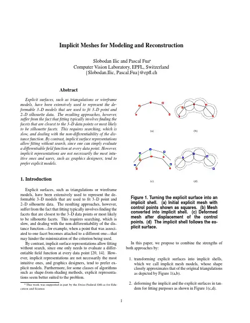
Implicit Meshes for Modeling and ReconstructionSlobodan Ilic and Pascal FuaComputer Vision Laboratory,EPFL,Switzerland{Slobodan.Ilic,Pascal.Fua}@epfl.chAbstractExplicit surfaces,such as triangulations or wireframemodels,have been extensively used to represent the de-formable3–D models that are used tofit3–D point and2–D silhouette data.The resulting approaches,however,suffer from the fact thatfitting typically involvesfinding thefacets that are closest to the3–D data points or most likelyto be silhouette facets.This requires searching,which isslow,and dealing with the non-differentiability of the dis-tance function.By contrast,implicit surface representationsallowfitting without search,since one can simply evaluatea differentiablefield function at every data point.However,implicit representations are not necessarily the most intu-itive ones and users,such as graphics designers,tend toprefer explicit models.1.IntroductionExplicit surfaces,such as triangulations or wireframemodels,have been extensively used to represent the de-formable3–D models that are used tofit3–D point and2–D silhouette data.The resulting approaches,however,suffer from the fact thatfitting typically involvesfinding thefacets that are closest to the3–D data points or most likelyto be silhouette facets.This requires searching,which isslow,and dealing with the non-differentiability of the dis-tance function—for example,when a point that was associ-ated to one facet becomes attached to a different one—thatmay hinder the minimization of the criterion being used.By contrast,implicit surface representations allowfittingwithout search,since one only needs to evaluate a differ-entiablefield function at every data point[20,14].How-ever,implicit representations are not necessarily the mostintuitive ones,and graphics designers,tend to prefer ex-plicit models.Furthermore,for some classes of algorithmssuch as shape-from-shading methods,explicit representa-tions seem better suited to the problem.Figure 2.Reconstruction from an uncalibrated video sequence.Top row:3of 6images from a short video sequence with overlaid silhouettes.Middle row:Disparity maps extracted from rectified consecutive image pairs using max flow-based stereo,after automated registration.Bottom row:Reconstructed and textured models obtained by using an explicit model for the head and an implicit mesh model for the neck and shoulders.To create the implicit shell,we circumscribe each facet with a spherical volumetric primitive.We will show that,if the triangulation is sufficiently well-behaved,the resulting shell closely approximates the mesh.To deform both representations simultaneously,we fol-low the Free Form Deformation (FFD)paradigm that lets us embed both kinds of models in a volume whose shape can be changed by moving control points.In particu-lar,we advocate the use of Dirichlet Free Form Defor-mations (DFFDs)[12]because,unlike conventional FFDs,they do not require the control points to lie on a regular rectangular grid.This is achieved by replacing the standard rectangular local coordinates by generalized natural neigh-bor coordinates,also known as Sibson coordinates [18].It gives us the ability to place control points at arbitrary loca-tions rather than on a regular lattice,and thus,much greater flexibility.In practice,control points are taken to be on the surface triangulation,with a denser distribution where the surface curvature is high.Our contribution is therefore an approach to surface fit-ting that allows us to take an arbitrary explicit surface model,for example one that has been obtained from the web and was not designed with fitting in mind,turn it into an im-plicit shell,and deform it to obtain an optimal least-square fit to new experimental data using a few well-chosen con-trol points.In Figure 2,we demonstrate the power of this approach for upper-body modeling using stereo and silhou-ette data.The model we use has a complex topology,but that complexity has no impact on the quality of the fitting.We first relate our techniques to existing ones.We then introduce our approach to creating implicit shells and to de-forming them using DFFDs.Finally,we demonstrate the applicability of our framework.2.Related Work2.1.Explicit versus ImplicitThree-dimensional reconstruction of visible surfaces continues to be an important goal of the computer visionresearch community and many approaches relying on full 3–D explicit representations have been proposed,such as3–D surface meshes[4,23],parameterized surfaces[19,11], local surfaces[6],and particle systems[21].In parallel,there has also been sustained interest in the vision community in the use of volumetric primitives[13, 10,22]and implicit surface representations[5,20,15].In the computer graphics community,approaches to interpo-lating explicit surfaces with implicit ones using radial ba-sis functions(RBF)have been proposed[3,24].However, the shape is controlled not only by the position of the RBF centers but also by the RBF weights that have no geometric interpretation,which makes this approach unsuitable for the kind of optimization we contemplate here.This is why we have developed a different approach to converting explicit surfaces into implicit shells that guarantees that the implicit shell’s shape deforms exactly in the same way as the explicit surface.Both approaches to3–D modeling have their strengths and weaknesses for the purpose offitting noisy image-data. Explicit surfaces are easy to deform and to render using well known computer graphics techniques,but as discussed earlier,are not ideal forfitting purposes.Implicit surfaces are better suited for least-squares stylefitting purposes be-cause they can be used to define differentiable objective functions[20,14].However,unless one uses either a sin-gle geometric primitive or a set of such primitives attached to some kind of skeleton,it is relatively difficult to control their shape in an intuitively pleasing way.As a result users such as graphics designers tend to prefer explicit models.It is therefore important to be able to go back and forth be-tween the two kinds or representations.2.2.Deforming the SurfacesFree Form Deformations(FFDs)are a well-known ap-proach to deforming3–D models,explicit or implicit,by warping the space in which they exist[17].However,a se-rious restriction is that FFDs can be naturally applied only to explicit surfaces and to parametric implicit surfaces such as quadrics or superquadrics.There is no generally accepted way to handle more complex implicit surfaces such as the implicit shells we are dealing with in this paper.Another popular and closely related way to deform implicit surfaces is to twist,bend,and taper the space in which the model lives by choosing a suitable warping function[1,25,2]. But,again,this only works for implicit surfaces with para-metric descriptions.Because the shape of the implicit shell depends only on the shape of the explicit surface it is derived from,we can use any Free Form Deformation technique.Here we advo-cate the use of Dirichlet Free Form Deformations[12].In previous work[8],we showed that it is effective tofit ex-plicit surfaces to noisy data.In this paper,we extend our earlier approach so that it can handle both explicit and im-plicit surfaces.3.Implicit Mesh ModelsTo create an implicit surface model that can deform in tandem with the explicit surface,we must address two prob-lems:1.Creating an implicit shell that closely approximates theshape of the initial explicit mesh,2.Controlling the object shape,in both its explicit andimplicit forms,using the same set of parameters.Our approach is depicted by Figs.1and3.We now discuss its components.3.1.From Explicit Surface to Implicit ShellWefirst build an implicit shell whose shape approxi-mates the initial explicit mesh as follows.We circumscribe a spherical metaball primitive around each facet of the sur-face triangulation in such a way that the sphere center lies on the facet as shown in the upper row of Fig.3.Ideally, to get a smooth implicit surface,the explicit mesh should have equally sized facets.In practice,the smaller the facets, the smaller the spheres circumscribed around them,and the closer the resulting implicit mesh approximates the initial explicit mesh.We have therefore found experimentally that subdividing the explicit mesh until all the facets are small enough is sufficient to produce visually pleasing results. The bottom row of Fig.3depicts the conversion of a simple regular triangulation patch into an implicit mesh.Further-more,as will be discussed below,the number of control pa-rameters does not depend on the number of primitives and there is no significant computational penalty in so doing.3.2.Deforming Explicit MeshesWe have shown in earlier work that introducing DFFD control points is an effective way to deform explicit meshes[8].These points can be distributed freely in space and every surface triangulation point is influenced by cer-tain subset of control points.The magnitudes of these in-fluences,known as Sibson coordinates[18],are computed before the optimization starts[12].The displacement of each surface triangulation point is the linear combination of the displacements of the control points that influence it.Let be the set of control points and be a subset influencing surface triangulation point ,,where.The elementsFigure3.Converting an explicit surface intoan implicit mesh.Upper row:Single trian-gular primitive on the left,converted to thetransparent spherical metaball primitive onthe right.Bottom row:Regular explicit sur-face patch on the left,converted to the trans-parent implicit mesh on the rightof are the natural neighbors of and their influence is expressed by the Sibson coordinates.Let the control points from be displaced from their initial positions by.The new position of the surface trian-gulation point becomes:(1) with and.3.3.Deforming Implicit MeshesOur goal is to deform the implicit mesh in tandem with the explicit meshes.Each spherical primitive being circum-scribed around a facet so that its center lies on the facet, both its center and its radius depend only on the facet ver-tices.These locations,in turn,can be expressed as a func-tion of the DFFD control points of Eq.1.We can therefore write thefield function that defines the implicit shell as(2)where is a point in,is one of thefield functions discussed below,is the Euclidean distance to the center of primitive,and is the radius of primitive and is the number of spherical metaballs.Note that,number of param-eters is the number of control points and does not depend on number of facets.We experimented with two different potentialfield functions.Thefirst one is piecewise polyno-mial:The parameter of Eq.3controls the zone of influ-ence of the primitives.As decreases,the zone’s size be-comes larger and the resulting implicit surface grows both smoother and larger,as shown on the top graph of Fig.4.On the contrary when increases,the zone of influence be-comes smaller and the implicit surface approximates more closely the explicit mesh.This function is good from a com-putational point of view,because the potential for a partic-ular 3–D point can be calculated only from the subset of primitives spheres in whose zone of influence it belongs.However,for fitting purposes,this can cause problems when the initial model is not close enough from the data that can then end up being completely ignored.Therefore,we use instead an exponential potential field function:(4)It has properties similar to those of the polynomial func-tion from Eq.3,except for the fact that its influence is infi-nite.In this way,we eliminate the risk of ignoring impor-tant 3–D points,at the cost of an increased computationalburden.As shown on the bottom graph in Fig.4,the pa-rameter acts again as smoothing parameter.Given the fact that this function decreases quickly,when the model is close enough to the data,we can speed up the computation by introducing an adaptive threshold on the distance above which the function does not need to be evaluated.4.Fitting to NoisyDataFigure 5.Generic model of the upper body and corresponding control mesh.Left:Complete model surface triangulation,with rigid head as a mesh and deformable neck-shoulders converted to the implicit surface.Right:Complete control meshOur goal is to deform the implicit mesh so that it con-forms to the image data which is made of 3–D points de-rived from stereo and silhouette information.In standardleast-squares fashion,for each data-point ,we write anobservation equation of the form(5)with weight,where is one of the possible types of observations we use,is a state vector that defines the surface shape,is the distance from the point to the surface,and is the deviation from the model.In practice,we taketo be the algebraic distance of to the implicit sur-face defined by the field function of of Eq.2and we mini-mize the weighted sum of the squares of the deviations.To ensure that the minimization proceeds smoothly,the systemautomatically computes theweights so that the differ-ent kinds of observations have commensurate influence[8].5.Parametrization and RegularizationIn theory we could take the parameter vector to be the vector of all ,and coordinates of the surface trian-gulation.However,because the image data is very noisy,we would have to impose very strong regularization con-straints.This is why we chose to use the DFFD approach to deforming the surface instead and introduce control trian-gulations such as the one depicted by Fig..5.Their vertices are points located at characteristic places on the model and serve as DFFD control points.This ability to place the con-trol points at arbitrary locations is what sets DFFDs apart from all other kinds of FFDs.The control triangulation facets are used to introduce the regularization constraint discussed below.In our scheme,we take the state vector to be the vector of 3-D displacements of DFFD control points[8].Because there are both noise and gaps in the image data,we still found it necessary to introduce a small regulariza-tion term.Since,we expect the deformation between the initial shape and the original one to be smooth,this can be done by preventing deformations at neighboring vertices of the control mesh to be too different.This is enforced by introducing a deformation energy that approximates the sum of the square of the derivatives of displacements across the control surface.By treating the control triangulation facets as finite elements,we write(6)where is a stiffness matrix and and are the vectors of the x,y and z coordinates of the control vertices’displacements.The term we actually optimize becomes:whereis a small positive constant.(a)(b)(c)Figure6.Synthetic example.(a)Initial state–implicit mesh model in light-grey,outline of the surface tofit shown as a white curve,stereo data shown as white dots.The thick white dot represents silhouette data that is perpendicular to the image plane.(b)Fitting results using stereo alone(c) Fitting using both stereo and silhouette data.6.Stereo and Silhouette ObservationsIn this work,we concentrate on combining stereo and silhouette data.Because thefield-function of Eq.2is both well-defined and differentiable,the observations and their derivatives can be computed both simply and without search.3–D Point Observations Disparity maps are used to com-pute clouds of noisy3–D points such as those of Fig.2.Each one is used to produce one observation of the kind described by5.Minimizing the corresponding residuals tends to force thefitted surface to be as close as possible to these points. Because of the long range effect of the exponentialfield function in the error function of Eq.2,thefitting succeeds even when the model is not very close to the data.Also, during least-squares optimization,an error measure that ap-proaches zero instead of becoming even greater with grow-ing distance has the effect offiltering outliers.Silhouettes Observations A silhouette point in the image defines a line of sight tangential to the surface.Let be an element of the state vector.For each value,we define the implicit surface:(7) Let be the point on the line of sight where it is tan-gential to.By definition,it must satisfy the two con-straints:1.The point is on the surface,therefore2.The normal to is perpendicular to the line of sightat.We integrate silhouette observations into our framework by performing,before each minimization,a search along the line of sight tofind the point that has the lowestfield value and,therefore,satisfies the second constraint.It is then used to add one of the observations described by5to enforce the first constraint.7.ResultsWefirst demonstrate our technique on a synthetic exam-ple and,then,show its applicability to modeling and track-ing people’s neck and shoulders.Synthetic Example We created a synthetic example that simulates a difficult situation in which one must combine stereo and silhouette data to achieve a good result.In the Fig.6(a),the initial state is depicted.The implicit mesh model is shown in light-grey.The outline of the synthetic surface we want tofit appears as a white curved line.To make the problem realistic,we assume that we have stereo data,shown as white dots,only on the front side of the patch,that is the one that faces the camera,and silhouette data at the top is shown as the thick white dot,that repre-sents the projection of the silhouette that is perpendicular to the image plane.The Fig.6(b)depicts the result offitting using stereo alone.Note that,the occluding contour of the deformed surface does not match the expected silhouette, again shown as a thick white dot.The Fig.6(c)depicts the result using both stereo and silhouette data.The occludingcontour of the fitted surface is now where it should be and the top of the surface has moved appropriately.The back of the shape is,of course,still inaccurate since there is neither silhouette nor stereo data to constrainit.Figure 7.Reconstructed shaded model with overlaid silhouettes.Top row:Reconstructed model using stereo alone viewed using the same perspective as that of the original im-ages from Figure 2and with overlaid silhou-ettes extracted from original images.Bottom row:Equivalent results using both stereo and silhouette data.Neck and Shoulder Modeling Here we show a similar behavior,but now using real stereo and silhouette data re-constructed from an initially uncalibrated 6–frame video se-quence in which the camera was moving around a static subject.In the top row of Fig.2,we show the first,mid-dle and last frames of the sequence.We used snakes to ex-tract the silhouettes shown as white lines.In the absence of calibration information,we used a model-driven bundle-adjustment technique [7]to compute the relative motion and,thus,register the images.We then used a graph-cut technique [16]to derive disparity maps from consecutive image ,such as those shown in the second column.Fi-nally,in the third column we show reconstructed textured model.Fig.7depicts reconstruction results of the neck and shoulders obtained either by using stereo alone or by using both stereo and silhouettes.In both cases,the head was reconstructed separately using our earlier DFFD-based method [8].As in the synthetic example,it is only when we combine both information sources that we get a model that projects correctly in all the views.This shows that itsshape is geometrically correct even at places where the sur-face slants away from the cameras and,therefore,where stereo fails.Note that the texture-mapped views of Fig.2and the shaded views of Fig.7were generated by moving the initial explicit surface to match the deformed implicit shell,thereby underlining the importance to go back and forth from the explicit to the implicitrepresentation.Figure 8.Tracking results for a short 21frames video sequence.Left column:Real images of 1st,11th and 21st frame with over-laid neck and shoulder model.Right column:View from above of the deformed model over-laid on the reprojected stereo data.Handling Deformations Finally,we tested our approach on a short stereo-video sequence in which we tracked the shoulder motion movement of a subject person moving his arms.In the left column of Fig.8,we show three images from the 21frame sequence we used on which we overlaid the neck and shoulder model we recovered for each frame.The model precisely follows the silhouettes of the neck and shoulders and shrinks when the arms move forward.On the right column of Fig.8,we show corresponding views from above in which we overlay the models on reprojected stereo data.The shoulders are aligned with the stereo data and,even though there is no large shoulder motion,we can spot a subtle deformation of both shoulders.8.ConclusionWe have presented an approach to switching from ex-plicit surfaces to implicit ones and back that allows us to take advantage of the strengths of both kinds of approaches. To this end,we have proposed a technique for creating im-plicit shells in such a way that their shape depend only on the explicit surface’s shape and a method based on Dirich-let Free Form Deformations for deforming the implicit and explicit models in tandem.We used the example of upper-body modeling using stereo and silhouette data to demonstrate the power of this approach.The explicit model we started from was not tai-lored forfitting purposes has man facets and a complex topology,neither of which has a significant impact on the quality of thefitting or the complexity of the computation.Our next step will be to explore the use of general-ized metaballs[9]representations in addition to the current spherical primitives.This will allow us to handle com-pletely general meshes without restriction on their facet sizes.We expect this to result in a completely generic tool for handling arbitrary explicit surface topologies.References[1] A.H.Barr.Global and local deformations of solid prim-itives.In Proceedings of the11th annual conference on Computer graphics and interactive techniques,pages21–30,1984.[2]J.F.Blinn.A Generalization of Algebraic Surface Drawing.ACM Transactions on Graphics,1(3):235–256,1982. [3]J.C.Carr and R.K.Beatson.Reconstruction and Repre-sentation of3D Objects with Radial Basis Functions.In SIGGRAPH,Los Angeles,CA,August2001.[4]I.Cohen,L.D.Cohen,and N.Ayache.Introducing newdeformable surfaces to segment3D images.In Conference on Computer Vision and Pattern Recognition,pages738–739,1991.[5]M.Desbrun and M.Gascuel.Animating Soft Substanceswith Implicit Surfaces.SIGGRAPH,pages287–290,1995.[6] F.P.Ferrie,garde,and P.Whaite.Recovery of V olu-metric Object Descriptions from Laser Rangefinder Images.In European Conference on Computer Vision,Genoa,Italy, April1992.[7]P.Fua.Regularized Bundle-Adjustment to Model Headsfrom Image Sequences without Calibration Data.Inter-national Journal of Computer Vision,38(2):153–171,July 2000.[8]S.Ilic and ing Dirichlet Free Form Deforma-tion to Fit Deformable Models to Noisy3-D Data.In Eu-ropean Conference on Computer Vision,Copenhagen,Den-mark,May2002.[9]X.Jin,Y.Li,and Q.Peng.General Constrained DeformationBased on Generalized puters and Graphics, 24(2):219–231,2000.[10]I.Kakadiaris and D.Metaxas.Model based estimation of3d human motion with occlusion based on active multi-viewpoint selection.In Conference on Computer Vision and Pattern Recognition,San Francisco,CA,June1996. [11] D.G.Lowe.Fitting parameterized three-dimensional mod-els to images.IEEE Transactions on Pattern Analysis and Machine Intelligence,13(441-450),1991.[12]L.Moccozet and N.Magnenat-Thalmann.Dirichlet Free-Form Deformation and their Application to Hand Simula-tion.In CA,1997.[13] A.Pentland and S.Sclaroff.Closed-form solutions for phys-ically based shape modeling and recognition.IEEE Transac-tions on Pattern Analysis and Machine Intelligence,13:715–729,1991.[14]R.Plänkers and P.Fua.Articulated Soft Objects for Video-based Body Modeling.In International Conference on Com-puter Vision,pages394–401,Vancouver,Canada,July2001.[15]R.Plänkers and P.Fua.Tracking and Modeling People inVideo puter Vision and Image Understand-ing,81:285–302,March2001.[16]S.Roy and I.J.Cox.A Maximum-Flow Formulation of theN-camera Stereo Correspondence Problem.In International Conference on Computer Vision,pages492–499,Bombay, India,January1998.[17]T.Sederberg and S.Parry.Free-Form Deformation of SolidGeometric Models.SIGGRAPH,20(4),1986.[18]R.Sibson.A vector identity for the Dirichlet Tessellation.InMath.Proc.Cambridge Philos.Soc.,pages151–155,1980.[19] E.M.Stokely and S.Y.Wu.Surface parameterization andcurvature measurement of arbitrary3-d objects:five prac-tical methods.IEEE Transactions on Pattern Analysis and Machine Intelligence,14(8):833–839,August1992. [20]S.Sullivan,L.Sandford,and ing geometricdistancefits for3–d.object modeling and recognition.IEEE Transactions on Pattern Analysis and Machine Intelligence, 16(12):1183–1196,December1994.[21]R.Szeliski and D.Tonnesen.Surface Modeling with Ori-ented Particle Systems.In Computer Graphics,SIGGRAPH Proceedings,volume26,pages185–194,July1992. [22] D.Terzopoulos and D.Metaxas.Dynamic3D models withlocal and global deformations:Deformable superquadrics.IEEE Transactions on Pattern Analysis and Machine Intelli-gence,13:703–714,1991.[23] D.Terzopoulos and M.Vasilescu.Sampling and reconstruc-tion with adaptive meshes.In Conference on Computer Vi-sion and Pattern Recognition,pages70–75,1991.[24]G.Turk and J.F.O’Brien.Shape transformation using vari-ational implicit surfaces.SIGGRAPH,pages335–342,Au-gust1999.[25] B.Wyvill and K.van Overveld.Warping as a modelling toolfor csg/implicit models.In Shape Modelling Conference, University of Aizu,Japan,pages205–214.IEEE Society Computer Press ISBN0-8186-7867-4,March1997.inivited.。
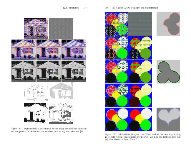
3Materials3.1Insulating Substrate and MetallizationThe insulating substrate serves as the supporting structure for the circuitry of the power module.1 It acts as the surface for depositing conductive, dielec-tric, and resistive materials that form the passive circuit elements. It is also a base for mechanical support for all active and passive chip components. It must be strong enough to withstand different environmental stresses. Electrically, it must be an insulator to isolate various conductive paths of the circuit. It must be able to withstand an RMS AC voltage (50 to 60 Hz) of 2500 V applied between any terminal and the case, including the base plate, for a one-minute duration. It must have sufficient thermal conductivity to remove the heat generated by the components.In addition, a high degree of surface smoothness is required for adhesion of films, fine conductor lines, and spacings. Surface flatness is desirable to minimize processing problems during screen-printing, photomasking, etc. Nonflat surfaces do not press uniformly against the base plate. This can potentially lead to microcracks and poor localized thermal conduction. 3.1.1Selection CriteriaThe substrate material most suitable for power applications should be determined by the following electrical, thermal, mechanical, and chemical requirements:2,3•Electrical–High-volume (or insulating) resistivity (> 1012W cm)–High dielectric strength (> 200 v/mil)–Low dielectric constant (< 15)•Thermal–High thermal conductivity (> 30 w/mK for effective thermal conduction)–Matching coefficient of thermal expansion with the power semi-conductor chips (2 to 6 ppm/°C for minimizing thermal stress and matching with Si 2.8 ppm/°C)–High thermal stability (> 1000°C for direct bonded copper [DBC] and brazing operations)•Mechanical–High tensile strength (> 200 MPa)–High flexural strength (> 200 MPa)–Dimensional stability — Hardness–Machineable — Can easily lap, polish, cut, and drill–Good surface finish (< 1 m m)—If not as fired, then should be able to be lapped to this specification–Metallizability — C ompatible with popular metallization tech-niques:•Thin film•Thick film•Plated copper•Direct bonded copper (DBC)•Active brazed copper (ABC)•Regular brazed copper (RBC)•Chemical–High resistance against acidic, alkaline, and other processing solvents–Low moisture absorption rate–Low toxicity–Chemically inert to plasma process•Density/weight–Low density/weight — Minimize mechanical shock •Maturity–Technology–Suppliers•Cost–As close to that of alumina as possible3.1.2List of Insulating SubstratesNumerous insulating substrates of different materials have been used for semiconductor applications.2-4 The following is a list of the popular ones, grouped by type:•Ceramic substrates–Alumina (Al2O3: 96%, 99%)–Aluminum nitride (AlN)–Beryllia (BeO)–Boron nitride (BN, hex)–Cordierite–Fordterite–Mullite–Steatite–Titanate•Glass substrate–Borosilicate glass•Sapphire substrate–Sapphire•Quartz substrate–Quartz•Si-based substrates–SiC–SiO2–Si3N4•Metal-core substrates–Insulated metal substrates (IMS)•Diamond substrate–Diamond (CVD polycrystalline)Table 3.1 through Table 3.5 show the following properties of these insu-lating substrates:1–20•Mechanical•Thermal•Electrical•Chemical•OtherTABLE 3.1Mechanical Properties of Insulating SubstratesMaterialTensileStrength(MPa)FlexuralStrength(MPa)ElasticModulus(GPa)HardnessSurfaceFinish(m m)Density(kg/m3)CeramicAl2O3(96%)127.4317310.32000 K 1.03970Al2O3(99%)206.93453459 MH 1.03970 AlN3103603101200 K 1.03260 BeO230250345100 K153000 BN (hex)1102200 Corderite5510141600 Forsterite55124902700 Mullite125175Steatite55110902500 Titanate2869693500 GlassBorosilicate509 1.02280 SapphireSapphire3994309 MH 1.03990 QuartzQuartz4814072 5 MH 1.02200 Si-basedSiC174404123160 SiO29630692190 Si3N4969323142400 Metal-coreIMS39262700 DiamondDiamond(CVD)100011807500 K< 1.03500 Note: MH = Moh; K = Knoop.TABLE 3.2Thermal Properties of Insulating SubstratesMaterialThermalConductivity(W/m ˚K)CTE(ppm/˚C)HeatCapacity(J/kg-˚C)MaximumUse Temperature(˚C )MeltingPoint(˚C)CeramicAl2O3(96%)24 6.0765********Al2O3(99%)337.276516002323 AlN150–180 4.6745> 10002677 BeO2707.010472725 BN (hex)60 3.8Corderite4 3.07701250Forsterite4111100Mullite6 4.2Steatite 2.510.51100Titanate410700GlassBorosilicate2 3.2SapphireSapphire41.77.3735QuartzQuartz43 5.581611401938 Si-basedSiC120 4.6675> 10003100 SiO2 1.50.6> 800Si3N470 3.0691> 10002173 Metal-coreIMS425DiamondDiamond (CVD)2000 (Z)1400 (X,Y)1509Resistant tooxidationto 600˚CTABLE 3.3Electrical Properties of Insulating SubstratesMaterial Resistivity(W-cm)DielectricStrength(kV/mm)DielectricConstantat 1 MHzCeramicAl2O3(96%)> 1014129.2Al2O3(99%)> 1014129.9 AlN> 1014158.9 BeO> 101412 6.7 BN (hex) 4.1 Corderite106–1014Forsterite1010–10127.9–11.8 6.2 Mullite> 1012Steatite1011–10137.9–15.7 5.5–7.5 Titanate106–1013 2.0–11.815 GlassBorosilicate> 1014 3.7 SapphireSapphire> 10144810.4 QuartzQuartz101016.1 3.8 Si-basedSiC> 101120–42 SiO2> 1014 3.5–4 Si3N4> 1010106–10 Metal-coreIMS> 1013DiamondDiamond(CVD)> 1011> 100 5.7TABLE 3.4Chemical Properties of Insulating SubstratesMaterialMoistureAbsorption(%)NitricAcidSulfuricAcid(Weight Loss atmg/cm2/day)CausticSoda ToxicityCeramicsAl2O3(96%)0NoAl2O3(99%)00.050.220.04No AlN0No BeO0Yes BN (hex)0No Corderite27No Forsterite0No Mullite5–15No Steatite0No Titanate0No GlassBorosilicate0No SapphireSapphire0000No QuartzQuartz0000No Si-basedSiC00.040.010No SiO20No Si3N40 1.000.400.36No Metal-coreIMS0No DiamondDiamond(CVD)0000NoTABLE 3.5Other Properties of Insulating SubstratesMaterial Metallizability a Machineability b Relative CostCeramicsAl2O3(96%)All, except thin film Good1¥Al2O3(99%)All Good2¥AlN All, except thickfilmGood4¥BeO All Good (only by approved source)5¥BN (hex)None GoodCorderite Thick film Good0.6¥Forsterite Thick film Good1¥Mullite Thick film Good1¥Steatite Thick film Good0.8¥Titanate Thick film Good2¥GlassBorosilicate Thin film Fair1¥SapphireSapphire Thin film Fair10¥QuartzQuartz Thin film Fair8¥Si-basedSiC None Fair4¥SiO2GoodSi3N4All Good 2.5¥Metal-coreIMS Thin and thickfilmsGoodDiamondDiamond (CVD)Thin and thickfilmsGood Higha Metallization: Thin film, thick film, plated copper, direct bonded copper (DBC), active brazed copper (ABC), regular brazed copper (RBC).b Machineability: lapping, polishing, cutting, drilling, shaping.3.1.3Selected Insulating SubstratesAfter carefully examining the preceding tables and comparing them with the selection criteria, it appears that there are four possible candidates for insulating material that are suitable for power semiconductor applications:•Ceramic substrates:–Al2O3 (96%, 99%)–AlN–BeO•Si-based substrate:–Si3N4CVD polycrystalline diamond substrate has promising potential if:•Heavy Cu metallization can be attached•Cost can be reducedIn the following sections, the strengths and weaknesses of each of these substrates are analyzed and compared.3.1.3.1Alumina (96%, 99%)•Strengths:–Most commonly used ceramic for substrate material and there-fore the most mature technology–Low cost — 1" ¥ 1" size as fired, 96% ~ $0.10; 99% ~ $0.20–Average but adequate all-around characteristics: mechanical, thermal, electrical, and chemical–Easily metallized — thin film, thick film, plated copper, DBC, ABC, RBC–Easily machineable–Nontoxic–Nonpermeable to gas–Zero moisture absorption rate–Camber ~ 0.003"/1"–Mature technology–Dimensionally stable•Weaknesses:–Thermal conductivity -30 w/k-m is adequate for low- to medi-um-power applications but ineffective for high power. Forexample, a 25-mil thick substrate with 10 mils of C u on bothsides and a 0.4" ¥ 0.4" IGBT chip attached to it has a thermalresistance of about 0.30 w/k-m. This means that for an acceptableT j rise of 30°C, the IGBT chip can only operate at 30 to 40A. Thischip is rated at about 75A and so is greatly underutilized.–Thermal expansion mismatch with Si — 6.0 to 7.2 ppm/ºC for Al2O3 vs. 2.8 ppm/°C for Si.–High dielectric constant.–Average chemical resistance ability against acid.•Comments:–More appropriate for low- to medium-power applications.–High-volume and low-cost applications.–Good material for hermetic packages.–For power applications, 99% Al2O3 is a better compromise be-tween cost and performance than the 96%.–If cost is an issue in the high-power application, then a very thin Al2O3 (10 mil) with 8 mils of Cu on both sides may be consideredas an alternative. In this case, the small thickness will compensatefor the low thermal conductivity of Al203. The trade-offs are inthe isolation voltage, V ISO, and in mechanical fragility.3.1.3.2Aluminum Nitride (AlN)•Strengths:–Very good thermal conductivity — Six times that of Al2O3–Very effective for high-power semiconductor applications–Good thermal expansion matching with Si — 4.6 ppm/°C for AlN vs. 2.8 ppm/°C for Si–Mechanical, thermal, and all other electrical characteristics are average but adequate (comparable to those of Al2O3)–Easily machineable–Nontoxic–Nonpermeable to gas–Zero moisture absorption rate–Inert to most chemicals–Camber ~ 0.003"/1"–Dimensionally stable–Relatively new material, so its technology is not as mature as Al2O3 and beryllia.–DBC metallization on AlN has difficulties. Thermal fatigue fail-ure is a major concern for DBC AlN substrate.–Thick-film metallization process is not as repeatable and reliable as Al2O3.–Four times more expensive than Al2O3.–Poor resistance against alkaline environment — Requires special cleaning agent.–May decompose into hydrated alumina in the presence of high temperature and humidity.•Comments:–One of the best all-around substrate materials for high-power semiconductor applications.–Due to its average mechanical fracture strength, it is preferred to be used in conjunction with a metal base plate. Otherwise, sub-strate thickness must be about 80 mils if it is exposed directly toexternal environment without a metal base plate.–Thermal fatigue capabilities depend very much on the following:•Bonding technique of Cu foil to the AlN substrate•Design of the Cu foil•Substrate thickness•Particular care must be exercised in selecting the right vendors. 3.1.3.3Beryllia (BeO)•Strengths:–Excellent thermal conductivity — Eight times that of Al2O3–Very effective for high-power semiconductor applications–Mature technology–Thermal, electrical, and all other chemical characteristics are av-erage, but adequate (comparable to those of Al2O3)–Easily metallized — Thin film, thick film, plated copper, DBC, ABC, and RBC–Nonpermeable to gas–Zero moisture absorption rate–Mature technology–Dimensionally stable–Toxic in both powder and vapor form:•Machining, such as cutting, drilling, and shaping, must be handled only by specialty vendors•Environmental issues are a major concern when disposing of the material–Limited suppliers–Thermal expansion mismatch with Si — 7.0 ppm/r C for BeO vs.2.8 ppm/r C for Si–Mechanical characteristics are below average, with mechanical strength only 60% that of Al2O3–Five times more expensive than Al2O3•Comments:–Used by the defense industry–For power semiconductor applications where thermal manage-ment consideration cannot be served in any other way3.1.3.4Silicon Nitride (Si3N4) — Sintered•Strengths:–Excellent thermal expansion match with Si — 3.0 ppm/r C for Si3N4vs. 2.8 ppm/r C for Si–Very strong mechanically:•Mechanical fractural toughness is more than double those of Al2O3and AlN, and triple that of BeO–Good thermal conductivity — Two-and-a-half times that of Al2O3–Effective for high-power semiconductor applications–Thermal and all other electrical characteristics are average but adequate (comparable to those of Al2O3).–Easily metallized — Thin film, thick film, plated copper, DBC, ABC, RBC–Easily machineable–Nontoxic–Nonpermeable to gas–Zero moisture absorption rate–Creep resistance–Good high-temperature strength–Good thermal shock resistance–Dimensionally stable–New material with relatively immature technology — Use of this material in the power semiconductor field is in the infancy stage.–Limited suppliers.–Weak chemical resistance against acidic environment.–Two to two-and-a-half times more expensive than Al 2O 3.•Comments:–Price will come down as usage increases.–Si 3N 4 is probably the best material to be used as a stand-alone substrate * (no metal base plate) for high-power semiconductor applications. It is also conceivable that power semiconductor chips can be attached to the top side of the substrate, with the bottom side having a finlike structure †formed or machined for the purpose of heat dissipation. In this way, the heat sink can be integrated directly with the substrate without the use of any mechanical force or thermal interface material.21–Good for applications where thermal fatigue capability is highly desired.Table 3.6 presents a list of suppliers for ceramic substrates.* Patent pending.†Patent pending.TABLE 3.6List of Substrate SuppliersSupplier96% Al 2O 399% Al 2O 3AlNBeO Si 3N 4Brush Wellman X X XCarborumdum X X XCeradyne X X XX CeramTec X X XCoors X X XCuramik X X X Denka X X X X Insaco X X KyoceraX X XX Lambertville X X NGK X X XStellar X XWesgo(Morgan Advanced Ceramics)XXXX3.1.4Metallization on Insulating SubstratesFor power semiconductor applications, the metallizations on the insulating substrates should possess the following characteristics:1,2,3,5,12,13•Thermal:–High thermal conductivity (> 200 w/k-m)–Matching thermal expansion with insulating substrate–High thermal fatigue capability — Greater than 1000 cycles from -40 to 100r C with no failures at the interface with the substrate –High thermal stability — Greater than 1000°C in order to be compatible with the direct bonding and brazing operations •Electrical:–Able to conduct high current density–Low electrical resistivity — Typically, ohmic drop across the met-allization should not exceed one-tenth of the IGBT’s V CESAT •Mechanical:–Strong adhesion to the substrate — High peeling strength–Al wire–bondable–Solderable for standard solder (such as 95Pb/5Sn, etc.)–Applicable to the previous four selected insulating substrates —Al2O3, AlN, BeO, and Si3N4–Compatible with standard processing equipment•Chemical:–Photoetchable — Designed pattern can be easily formed (for the case of thick film, this is not required)–High chemical resistance against standard processing solvents–Nontoxic–Good corrosion resistance–Chemically inert•Cost:–Low3.1.5 Types of Metallizations3.1.5.1Metallization TechnologiesThe insulating substrate is typically metallized by one of the methods listed in Table 3.7.TABLE 3.7Metallization TechnologiesThick Film Thin Film Copper Metallization Polymer Sputtering Plated copperCermet Evaporation Direct bonded copperGold Gold Active brazed copperSilver Silver Regular brazed copperCopper CopperPalladium silver AluminumPlatinum goldPlatinum silverRefractoryTungstenMolybdenumMoly-manganese3.1.5.2Types of Metallization2,33.1.5.2.1Thick FilmThick-film circuits are typically fabricated by screen-printing a specially formulated paste onto a substrate, which is dried and then fired at high temperature. The paste can be in the form of a conductor, resistor, capacitor, inductor, fuse, varister, transient voltage suppressor, or thermistor. Typical film thickness is from 0.5 to 2.0 mils.There are three basic categories of thick film:• Polymer• Cermet• Refractory3.1.5.2.1.1Polymer — Polymer thick film (PTF) is a polymeric resin mixed with conductive, resistive, or insulating particles. It is fired or cured at temperatures ranging from 85 to 300r C, typically from 120 to 165r C. It is low in cost, limited to low-temperature operation, and widely used in plastic or organic substrates.3.1.5.2.1.2Cermet — This is the most popular type and is applicable to both ceramic and Si-based substrates.It consists of a mixture of the following:•Active element — To establish the function of the film•Adhesion element — To provide adhesion to the substrate •Organic binder — To provide proper fluid properties for screen printing •Solvent or thinner — To adjust the viscosityThis mixture is fired at a range from 850 to 1000r C.TABLE 3.8Popular Thick Film MaterialsMaterial Resistively, r (m W/ )Gold3Silver1Copper2Palladium silver30Palladium gold50Platinum gold50The adhesion of the thick film to the substrate is above average, and the thermal fatigue capability is rated as fair.Popular thick film materials are shown in Table 3.8.The maximum current allowed for each type of material can be calculated from the following:•Cross-sectional area of the metallization•Maximum power dissipation allowed for each materialFor example:•Al2O3 substrate — 4 watt/cm2•BeO substrate — 80 watt/cm2•AlN and Si3N4 substrates are somewhere in betweenBecause the typical thick-film thickness is 0.5 mil or 12 m m, it can be seen that the maximum current-carrying capability is about a few amperes.3.1.5.2.1.3Refractory — These are special kinds of cermet thick film that can withstand high-temperature operations. They are typically fired at a much higher temperature (1500 to 1600r C) in a reducing atmosphere. The adhesion of these films to the substrates is strong, and the thermal fatigue capability is rated as very good. Popular refractory materials are tungsten and molybdenum (Table 3.9).The maximum current carrying capability is limited to 1 to 2 amperes for these materials.TABLE 3.9Popular Refractory MaterialsRefractory Material Resistively, r (m W/ )Tungsten22–32Molybdenum153.1.5.2.2 Thin FilmThin-film circuits are typically fabricated by first sputtering or evaporating the film across the entire surface of the substrate. This film is then coated, photoprocessed, and etched to form the desired pattern. Thin film offers better definition and narrower lines than thick film. It is most suitable for high-density and high-frequency applications. Thin film metallization adheres strongly to the substrate and provides excellent thermal fatigue performance. Wire bondability is also superior to that of thick film.Due to the labor and specialty equipment involved, thin-film circuits are almost five to six times more expensive than thick film. Also, multilayer thin-film structure is extremely difficult and expensive to fabricate. Popular thin-film materials include the following:•Gold•Silver•Copper•AluminumTypical thickness is about 0.1 mil (2.5 m m) or less. Current-carrying capa-bility is limited to a few amperes.3.1.5.2.3Copper MetallizationBoth thick-film and thin-film technologies are limited in their thickness, usually to less than 1 mil (25 m m). This limitation affects their ability to conduct large currents.Copper metallization technology provides three features:•Increased metallization thickness•Improved current-carrying capability•Improved thermal spreadingFour basic techniques are available:•Plated copper•Direct bonded copper (DBC)•Active brazed copper (ABC)•Regular brazed copper (RBC)However, as the copper metallization thickness increases, its thermal expansion mismatch with the insulating substrates becomes more and more pronounced, as shown in Table 3.10.This large mismatch will be manifested during thermal fatigue tests, which can potentially lead to excessive thermal stress and eventually to micro-cracks. Proper metallization design and processing techniques must beTABLE 3.10CTE of Insulating Substrates and Copper MetallizationMaterial CTE (ppm/°C)Al2O3(96%) 6.0AL2O3 (99%)7.2AlN 4.6BeO7.0Si3N4 3.0Cu17.0utilized to minimize or eliminate these cracks. This requires careful screening of suppliers.Copper has the additional problems of adhesion and being very chemically reactive. A barrier layer is required to improve adhesion, and a Ni or Au layer is required on the surface for protection.3.1.5.2.3.1Plated Copper — The concept behind this technique is to build up the thickness of copper material by electroplating. A film is first deposited onto the substrate, either by a thin-film method (sputtering or evaporation) or a thick-film process (screen-printing). Typical materials used are Moly/ Mn for thin film and copper for thick film. A layer of electroless copper may be plated over this film surface, followed by electrolytic copper to increase the thickness. The plated copper film is then fired at an elevated temperature in a nitrogen atmosphere to improve adhesion. The thermal fatigue strength of plated copper is rated as good. One supplier has successfully performed 1000 cycles from -55 to 150r C without failure for 4-mil thick plated Cu. Maximum copper thickness achievable after electroplating is about 5 to 8 mils, with density of about 70% of regular copper material. Fine patterns can be generated by photolithographic etchings. For thicker film, this may result in undercutting and loss of resolution. Current-carrying capability has been reported up to 50 A.3.1.5.2.3.2Direct Bonded Copper3,17,18 — This technique uses a high-tem-perature process to achieve an intimate bond between the copper and the ceramic. There is no solder or any other catalyst used in the interface between the copper and the ceramic surface. Here, the combination of copper and ceramic is heated to a temperature of about 1070r C, slightly below copper’s melting point, in a nitrogen atmosphere. At this temperature, the copper oxide forms a eutectic melt that wets and, when cool, produces a strong bond between copper and ceramic.Copper thickness is typically 8 to 20 mils, and patterns can be formed by photolithographic etching. Fine resolution is difficult due to undercutting. Minimum line width and separation are 20 mils. Copper is usually bonded to both surfaces of the substrate in order to balance thermal expansion.Because a layer of copper oxide is required for the direct bonding process, AlN and Si3N4 ceramics must be treated first in order to apply this technique. This involves an additional oxidation process at about 125°C. However, this added oxygen diffuses along grain boundaries and may downgrade the thermal conductivity of AlN and Si3N4.Direct bonded copper offers the following advantages for power packag-ing:•The copper and ceramic tend to act, often bonding, like an integral unit with a single coefficient of thermal expansion. This coefficientis much lower than that of pure copper and more closely matchedto that of the ceramic. It is therefore possible to solder even largechips directly onto the copper layer without risking stress damages.•The copper used is of the high-purity, oxygen-free high-conductivity (OFHC) type. With proper line width and thickness, the metalliza-tion can be of very low electrical resistance and can handle currentwell in excess of 100 A.•The thick layer of copper provides efficient heat spreading from the power chips.3.1.5.2.3.3Active Brazed Copper — The active brazed copper process uti-lizes brazing alloy to form a bonding layer between copper and ceramics.3,16 An example is the alloy of silver, copper, titanium, and zirconium in the ratio 72Ag/28Cu/3TiH2/3Zr.The braze is usually applied in the form of a paste. Most suppliers use the screen-printing technique. The resulting titanium braze layer provides supe-rior adhesion and thermal cycle performance.Active brazed copper has been applied extensively to AlN and lately to Si3N4 substrates, where DBC techniques have experienced difficulties. Dur-ing direct bonding operation on these ceramics, oxygen gas must be fed into the critical interface region. This added oxygen will diffuse along grains and reduce the thermal conductivity of the ceramics. Furthermore, the release of gases during the direct bonding process may require a perforated C u foil design. However, this results in a loss of conduction area for current. The advantages of using the ABC process over DBC for these two substrates are as follows:•Better adhesion•Better current-carrying capability•Better thermal-fatigue capability3.1.5.2.3.4Regular Brazed Copper — The technique is similar to that of the active brazed copper, except that it is performed in a vacuum. In this case, typically a thin silver film is first sputtered onto the substrate. Ag-braze alloy is then applied to the film in the form of a paste, and the copper foil is placedon top. The combination is then heated to the melting point of the braze alloy. After brazing, the top foil may be photoetched to form the desired pattern.One supplier noted that the titanium-based brazing alloy is overly active and can potentially lead to nonuniform brazing. Regular Ag-based braze is more controllable and therefore results in a more uniform and stronger adhesion.Table 3.11 and Table 3.12 compare different metallizations available for the insulating substrates.For a conductor of 40 mil width and 12 mil thickness on an Al 2O 3 substrate,the temperature rise for a 100 A operating current is about 17°C. From Table 3.11, we can conclude that the metallizations for high-power semiconductor applications are:•Direct bonded copper (DBC)•Active brazed copper (ABC)•Regular brazed copper (RBC) •Plated copper (possibly)An estimate of the total cost of the insulating substrate per square inch with metallizations at thickness of 25 mils is as shown in Table 3.13.3.1.6Analysis of Copper Metallization SuppliersIt should be noted that the preceding description of the technology is very general. Every supplier has its own unique processing features and design techniques that can affect performance, especially thermal fatigue and cost.Table 3.14 through Table 3.17 provide lists of suppliers and their capabilities.This information is gathered from publications, conferences, or private con-versations.TABLE 3.11Metallization for Different Insulating SubstratesTechnology Al 2O 3AlN BeO Si 3N 4Thin film Good Good Good Good Thick film Good FairGood FairPlated copper GoodGoodDB C Good GoodABC Good Good RBCGood GoodTABLE 3.12Comparison of Metallization Technologies4,5Technology Adhesion Geometry Process Electrical ThermalFatigueProcessCostThin film Good0.002 line< 0.005 thick Good wirebondability;fair solderability1–2 A Good HighThick film Fair0.010 line> 0.005 thick Good wirebondability;good solderability2–5 A Fair LowPlated copper Fair0.004 line0.005 thick Good wirebondability;good solderability50 A Fair MediumDBC Good0.020 linetyp 0.020 thick Good wirebondability;good solderability> 200 A a Good forAl2O3andBeOLowABC, RBC Good0.020 linetyp 0.020 thick Good wirebondability;good solderability> 200 A Good for AlNand Si3N4Lowa For a conductor of 40 mil width and 12 mil thickness on a A12O3 substrate, the temperature rise for 100 Amp. operating current isabout 17°C.© 2005 by CRC Press LLC。
Eurographics Symposium on Geometry Processing(2006)Konrad Polthier,Alla Sheffer(Editors)Poisson Surface ReconstructionMichael Kazhdan1,Matthew Bolitho1and Hugues Hoppe21Johns Hopkins University,Baltimore MD,USA2Microsoft Research,Redmond WA,USAAbstractWe show that surface reconstruction from oriented points can be cast as a spatial Poisson problem.This Poisson formulation considers all the points at once,without resorting to heuristic spatial partitioning or blending,and is therefore highly resilient to data noise.Unlike radial basis function schemes,our Poisson approach allows a hierarchy of locally supported basis functions,and therefore the solution reduces to a well conditioned sparse linear system.We describe a spatially adaptive multiscale algorithm whose time and space complexities are pro-portional to the size of the reconstructed model.Experimenting with publicly available scan data,we demonstrate reconstruction of surfaces with greater detail than previously achievable.1.IntroductionReconstructing3D surfaces from point samples is a well studied problem in computer graphics.It allowsfitting of scanned data,filling of surface holes,and remeshing of ex-isting models.We provide a novel approach that expresses surface reconstruction as the solution to a Poisson equation. Like much previous work(Section2),we approach the problem of surface reconstruction using an implicit function framework.Specifically,like[Kaz05]we compute a3D in-dicator functionχ(defined as1at points inside the model, and0at points outside),and then obtain the reconstructed surface by extracting an appropriate isosurface.Our key insight is that there is an integral relationship be-tween oriented points sampled from the surface of a model and the indicator function of the model.Specifically,the gra-dient of the indicator function is a vectorfield that is zero almost everywhere(since the indicator function is constant almost everywhere),except at points near the surface,where it is equal to the inward surface normal.Thus,the oriented point samples can be viewed as samples of the gradient of the model’s indicator function(Figure1).The problem of computing the indicator function thus re-duces to inverting the gradient operator,i.e.finding the scalar functionχwhose gradient best approximates a vectorfield V defined by the samples,i.e.minχ ∇χ− V .If we applythe divergence operator,this variational problem transforms into a standard Poisson problem:compute the scalar func-111F M00111Indicator functionF MIndicator gradient Surfacew M Oriented pointsVGFigure1:Intuitive illustration of Poisson reconstruction in2D.tionχwhose Laplacian(divergence of gradient)equals the divergence of the vectorfield V,∆χ≡∇·∇χ=∇· V.We will make these definitions precise in Sections3and4. Formulating surface reconstruction as a Poisson problem offers a number of advantages.Many implicit surfacefitting methods segment the data into regions for localfitting,and further combine these local approximations using blending functions.In contrast,Poisson reconstruction is a global so-lution that considers all the data at once,without resorting to heuristic partitioning or blending.Thus,like radial basis function(RBF)approaches,Poisson reconstruction creates very smooth surfaces that robustly approximate noisy data. But,whereas ideal RBFs are globally supported and non-decaying,the Poisson problem admits a hierarchy of locally supported functions,and therefore its solution reduces to a well-conditioned sparse linear system.模型的有向点集可以看作是指示函数的梯度的采样;很多的隐式曲面重建方都会将数据分成局部数据拟合。
收稿日期:2008-08-16基金项目:浙江省自然科学基金资助项目(Y )作者简介:苗兰芳(63),女,浙江慈溪人,副教授,博士,主要研究方向为基于点的建模和绘制。
2010年工程图学学报2010第2期J OURNAL OF ENG INEERING GRAPHICSNo.2稠密采样点模型的快速隐式曲面重建苗兰芳1,周廷方2,彭群生2(1.浙江师范大学信息科学与工程学院,浙江金华321004;2.浙江大学CAD&CG 国家重点实验室,浙江杭州310027)摘要:算法以稠密采样点模型表面局部区域内的双边滤波函数值为依据,模型表面附近任意一点的函数值通过与该点最近的模型表面的K 个采样点数据直接计算得到。
与已有的隐式曲面重建方法相比,该方法既不用曲面内部或外部的支撑点,也不用求解线性和非线性方程,其重建速度快。
此外,由于采用双边滤波函数作为其重建的隐式曲面的函数值,因此还能对带有噪声的采样点模型进行特征保持的表面重建。
实验结果表明,对于稠密采样点模型,该方法可以快速重建出逼近程度高,效果好的曲面。
关键词:计算机应用;隐式曲面重建;双边滤波函数;采样点模型中图分类号:TP 391文献标识码:A文章编号:1003-0158(2010)02-0084-08Fast Implicit Surface Reconstruction for Densely Sampled Point M odelMIAO Lan-fang 1,ZHOU Ting-fang 2,PENG Qun-sheng 2(1.Mathemati cs,Physics and Information Engineering College,Zhejiang Normal University,Jinhua Zhej iang 321004,China;2.State Key Lab of CAD&CG,Zhejiang University,Hangzhou Zhejiang 310027,C hina )Abstr act:The proposed algorithm uses the local bilateral filter function near the surface of the point model as the surface reconstruction function.The function value at a given position near the model surface can be computed directly by the bilateral filter function of the nearest pared with previous methods,this algorithm doesn ’t need solve any linear system or non-linear equations and doesn ’t need any internal or external support points.In addition,it can handle the noising data and preserve sharp features,since the function is based on a bilateral filter.Experiment results show that it can reconstruct high quality surfaces for complex 3D objects.K ey words:computer application;implicit surface reconstruction;bilateral filter;sampled point model10708419-现实世界中有许多应用有赖于建立准确的实体模型并进行可视化,如雕像、考古艺术品、大规模地貌以及反求工程中的模型仿制、模具翻新等。
Journal of Materials Processing Technology170(2005)11–16Application of response surface methodology in the optimizationof cutting conditions for surface roughnessH.¨Oktem a,∗,T.Erzurumlu b,H.Kurtaran ba Department of Mechanical Engineering,University of Kocaeli,41420Kocaeli,Turkeyb Department of Design and Manufacturing Engineering,GIT,41400Gebze,Kocaeli,TurkeyReceived16July2004;received in revised form12March2005;accepted12April2005AbstractThis paper focuses on the development of an effective methodology to determine the optimum cutting conditions leading to minimum surface roughness in milling of mold surfaces by coupling response surface methodology(RSM)with a developed genetic algorithm(GA). RSM is utilized to create an efficient analytical model for surface roughness in terms of cutting parameters:feed,cutting speed,axial depth of cut,radial depth of cut and machining tolerance.For this purpose,a number of machining experiments based on statistical three-level full factorial design of experiments method are carried out in order to collect surface roughness values.An effective fourth order response surface (RS)model is developed utilizing experimental measurements in the mold cavity.RS model is further interfaced with the GA to optimize the cutting conditions for desired surface roughness.The GA reduces the surface roughness value in the mold cavity from0.412m to0.375m corresponding to about10%improvement.Optimum cutting condition produced from GA is verified with the experimental measurement.©2005Elsevier B.V.All rights reserved.Keywords:Milling;Cutting conditions;Surface roughness;Injection molding;Response surface methodology;Genetic algorithm1.IntroductionRecent developments in manufacturing industry have con-tributed to the importance of CNC milling operations[1,2]. Milling process is required to make mold parts used for pro-ducing plastic products.It is also preferred in machining mold parts made of Aluminum7075-T6material.Aluminum7075-T6material as chosen in this study is commonly utilized in aircraft and die/mold industries due to some advantages such as high resistance,good transmission,heat treatable and high tensile strength[3,4].The quality of plastic products manufactured by plas-tic injection molding process is highly influenced by that of mold surfaces obtained from the milling process.Sur-face quality of these products is generally associated with surface roughness and can be determined by measuring sur-face roughness[5].Surface roughness is expressed as the irregularities of material resulted from various machining ∗Corresponding author.Tel.:+902627423290;fax:+902627424091.E-mail address:**************.tr(H.¨Oktem).operations.In quantifying surface roughness,average sur-face roughness definition,which is often represented with R a symbol,is commonly used.Theoretically,R a is the arith-metic average value of departure of the profile from the mean line throughout the sampling length[6].R a is also an important factor in controlling machining performance. Surface roughness is influenced by tool geometry,feed,cut-ting conditions and the irregularities of machining operations such as tool wear,chatter,tool deflections,cuttingfluid,and workpiece properties[7,11,16].The effect of cutting con-ditions(feed,cutting speed,axial–radial depth of cut and machining tolerance)on surface roughness is discussed in this study.Several researchers have studied the effect of cutting con-ditions in milling and plastic injection molding processes such as in vacuum-sealed molding process[5].Analytical models have been created to predict surface roughness and tool life in terms of cutting speed,feed and axial depth of cut in milling steel material[8,9].An effective approach has also been presented to optimize surfacefinish in milling Inconel 718[10].0924-0136/$–see front matter©2005Elsevier B.V.All rights reserved. doi:10.1016/j.jmatprotec.2005.04.09612H.¨Oktem et al./Journal of Materials Processing Technology170(2005)11–16In this study,a fourth order response surface(RS)model for predicting surface roughness values in milling the mold surfaces made of Aluminum(7075-T6)material is devel-oped.In generating the RS model statistical response surface methodology(RSM)is utilized.The accuracy of the RS model is verified with the experimental measurement.The developed RS model is further coupled with a developed genetic algorithm(GA)tofind the optimum cutting condition leading to the least surface roughness value.Cutting condition is represented with cutting parameters of feed,cutting speed, axial–radial depth of cut and machining tolerance.The pre-dicted optimum cutting condition by GA is validated with an experimental measurement.The RS model and GA developed and utilized in this study present several advantages over other methods in the litera-ture.The RS model is a higher order and more sophisticated polynomial model with sufficient accuracy.The GA elimi-nates the difficulty of user-defined parameters of the existing GAs.Details of the RS model generation by RSM and the optimization process by GA are given in the following sec-tions.2.Experimental procedures2.1.Plan of experimentsAn important stage of RS model generation by RSM is the planning of experiments.In this study,cutting experi-ments are planned using statistical three-level full factorial experimental design.Cutting experiments are conducted con-sideringfive cutting parameters:feed(f t),cutting speed(V c), axial depth of cut(a a),radial depth of cut(a r)and machin-ing tolerance(m t).Overall35=243cutting experiments are carried out.Low–middle–high level of cutting parameters in cutting space for three-level full factorial experimental design is shown in Table1.Ranges of cutting parameters are selected based on recommendation of Sandvik Tool Catalogue[12]. Milling operations are performed at the determined cutting conditions on a DECKEL MAHO DMU60Pfive axis CNC milling machine.Surface roughness(R a)values are measured from the mold surfaces.2.2.Tool and materialCutting tool used in experiments has the diameter of 10mmflat end mill with four teeth.The material of the tool Table1Low–middle–high levels of cutting parameters in three-level full factorial design of experimentCutting parameters Three-level values Feed,f t(mm/tooth)0.08–0.105–0.13 Cutting speed,V c(m/min)100–200–300 Axial depth of cut,a r(mm)0.3–0.5–0.7 Radial depth of cut,a r(mm)1–1.5–2 Machining tolerance,m t(mm)0.001–0.0055–0.01Fig.1.Mold part.is PVD AlTiN coated with solid carbide.It has the helix angle of45◦and rake angle of10◦.Machining experiments are performed in the mold cavity on aluminum(7075-T6) block with dimensions of120mm×120mm×50mm.The chemical composition of workpiece material is given in the following specification(wt.%):1.6Cu,2.5Mg,0.23Cr,5.40 Zn.The hardness of workpiece is measured as150BHN. The mechanical properties of aluminum material are:ten-sile strength of570MPa,yield strength of505MPa,shear strength of330MPa and elongation of11%.Surface roughness is measured with Surftest301pro-filometer at traverse length of2.5mm along centerline of sam-pling.Converting the measurement into a numerical value, mathematical definition of R a is used.Since this way of con-version is common in the literature it is adopted in this study as well[7–9].Each R a measurement is repeated at least three times.Average of three R a values is saved to establish RS model.2.3.Mold partsThe mold part used in this study is utilized to produce the components of an orthose part in biomechanical appli-cations.It is shown in Fig.1.Orthose parts are generally utilized in walking apparatus that holds human legs in stable position during walking.It binds the kneecap region of leg and is equipped with cylindrical bars that are made of alu-minum material in diameter of12mm and length of300mm. Orthose part consists of three main components;one of them is employed as the working model in this study.2.4.Manufacturing the components of orthose partThree machining processes are implemented in order to manufacture each component of the orthose part in an inte-grated manner.Firstly,the selected component is machined in CNC milling machine.R a values are then taken from the sur-faces in the mold cavity.Secondly,plastic product is injectedH.¨Oktem et al./Journal of Materials Processing Technology170(2005)11–1613Fig.2.The parts obtained from three machiningprocess.Fig.3.The stages taken in creating a response surface model by RSM. in plastic injection machine produced by ARBURG.Poly-acetal(POM)C9021material is used to inject the polymer material.The properties of polymer material has the den-sity of solution1.2g/cm3,the ejected temperature of165◦C, viscosity of50Pa s and meltflow-fill rate of0.8cm3/min. Finally,net casting process is applied for producing die cast-ing part.Mold part,plastic product and die casting part are illustrated in Fig.2.3.Response surface model for surface roughnessRS model,which is an analytical function,in predicting surface roughness values is developed using RSM.RSM uses statistical design of experiment(experimental design)tech-nique and least-squarefitting method in model generation phase.It is summarized in Fig.3.RSM was originally devel-oped for the modelfitting of physical experiments by Box and Draper[13]and later adopted in otherfields.RS model is formulated as following polynomial function:f=a0+ni=1a i x i+ni=1nj=1a ij x i x j+ (1)where a0,a i and a ij are tuning parameters and n is the number of model parameters(i.e.process parameters).In this study, to create RS model,a computer program has been written in MATLAB programming language.The RS program developed has the capability of creat-ing RS polynomials up to10th order if sufficient data exist. All cross terms(i.e.interactions between parameters)in the models can be taken into account.RS models can also be generated in terms of inverse of parameters.That is,x i can be replaced as1xi(i.e.inversely)in RS model if desired,in creating the RS models,243surface roughness values deter-mined based on three-level full factorial experimental design forfive parameters(f t,V c,a a,a r and m t)are used The243 data sets for surface roughness are divided into two parts; training data set and the check(i.e.test)data set.Training data set includes236surface roughness values and is uti-lized in modelfitting procedure.Because of large number of values and to save space,training data is shown in Fig.4, rather than in a table.In Fig.4,abscissa indicates the data set number and the ordinate indicates the corresponding sur-face roughness value.Check data sets include seven surface roughness values and are used in checking the accuracy of the RS model.Check data sets are shown in Table2.They parison of experimental measurements with RS prediction for surface roughness.14H.¨Oktem et al./Journal of Materials Processing Technology 170(2005)11–16Table 2The data set used for checking the accuracy of RS model Set numberCutting conditions R a (m)f tV c a a a r m t Measurement results RSM model Maximum test error (%)10.1052000.710.0010.5910.589 2.0520.1052000.7 1.50.0010.6290.62730.1052000.310.00550.7810.77540.082000.7 1.50.00550.8990.89550.081000.720.00550.9780.99660.082000.3 1.50.01 1.674 1.70670.1052000.520.011.8561.893Table 3The accuracy error of several RS models Reciprocal flag First order Second order Third order Fourth order [00000]277 4.8 2.7[00100]25.97.28 5.8 2.95[00001]52.410.9 4.0 2.99[11000]27.2 6.63 4.8 2.05[01100]25.97.0 5.5 2.55[00011]54.910.5 3.7 2.7[11100]25.87.03 5.7 2.5[01110]27.57.0 5.9 2.8[11111]53.0310.54.72.7are selected from 243data sets to show a good distribution in the cutting parameters’space and thereby to have a good check on the accuracy of the RS model.In this study,RS models of varying orders from first order to fourth order are created and tested with the developed program.Several RS model created are demonstrated along with their accuracy errors in Table 3.In reciprocal section in Table 3,0indicates a parameter (x i ),1indicates the inverse ofa parameter (1x i ).The full fourth order polynomial function of the form:R a =a 0+a 11f t +a 21V c +a 3a a +a 4a r +a 5m t +···+a n 1f t 1V ca a a r m t 4+···+a m (m t )4(2)fits best (with minimum fitting error)to the training data set.The accuracy of the RS model was checked using the check data set.The maximum accuracy error is found to be about 2.05%.This indicates that RS model generated has sufficient accuracy in predicting surface roughness within the range of cutting parameters.4.Optimization of cutting conditions for surface roughness4.1.Optimization problem formulationSince it is indicator of surface quality in milling of mold surfaces,surface roughness value is desired to be as low as possible.Low surface roughness values can be achieved effi-ciently by adjusting cutting conditions with the help of an appropriate numerical optimization method.For this,mini-mization of surface roughness problem must be formulated in the standard mathematical format as below:Find :f t ,V c ,a a ,a r ,m t(3a)Minimize :R a (f t ,V c ,a a ,a r ,m t )(3b)Subjected to constraints :R a ≤0.412m (3c)Within ranges :0.08mm ≤f t ≤0.13mm 100mm ≤V c ≤300mm 0.3mm ≤a a ≤0.7mm 1mm ≤a r ≤2mm 0.001mm ≤m t ≤0.01mm .In Eq.(3),R a is the RS model developed in Section 3.f t ,V c ,a a ,a r and m t are the cutting parameters.In the opti-mization problem definition above,a better solution is also forced through the constraint definition.Constraint definition searches a surface roughness value (R a ),which is less than the lowest value in 243data set if possible.Minimum surface roughness value in 243data set is 0.412m.The ranges of cutting parameters in optimization have been selected based on the recommendation of Sandvik Tool Catalogue.4.2.Optimization problem solutionThe optimization problem expressed in Eq.(3)is solved by coupling the developed RS model with the developed genetic algorithm as shown in Fig.5.The genetic algorithm [14]solves optimization problem iteratively based oh biological evolution process in nature (Darwin’s theory of survival of the fittest).In the solution pro-cedure,a set of parameter values is randomly selected.Set is ranked bashed on their surface roughness values (i.e.fitnessFig.5.Interaction of experimental measurements,RS model and GA during surface roughness optimization.H.¨Oktem et al./Journal of Materials Processing Technology170(2005)11–1615Table4GA parametersSubject Values Population size50 Crossover rate 1.0 Mutation rate0.1 Number of bit16 Number of generations540values in the GA literature).Best combination of parameters leading to minimum surface roughness is determined.New combination of parameters is generated from the best com-bination by simulating biological mechanisms of offspring, crossover and mutation.This process is repeated until sur-face roughness value with new combination of parameters cannot be further reduced anymore.Thefinal combination of parameters is considered as the optimum solution.The criti-cal parameters in GAs are the size of the population,mutation rate,number of iterations(i.e.generations),etc.and their val-ues are given in Table4.The GA written in MATLAB programming language selects chromosomes based on the objective value and the level of constraint violation.Fitness values of the popula-tion are biased towards the minimum objective value and the least infeasible sets in offspring phase.Most of GAs in the literature converts the constrained optimization problem into an unconstrained optimization problem through penalty function before the solution.This brings the difficulty of appropriate selection of problem dependent penalty coeffi-cient which requires user experience.In the program used in this study,this difficulty is avoided since no problem depen-dent coefficient is needed[15].4.3.Optimization results and discussionBy solving the optimization problem,the GA reduces the surface roughness of mold surfaces from0.412m to 0.375m by about10%compared to the initial cutting con-dition.The best(optimum)cutting condition leading to the minimum surface roughness is shown in Table5.The pre-dicted optimum cutting condition by GA is further validated with a physical measurement.Predicted surface roughness value is compared with the measurement in Fig.6.From Table5The best cutting conditionParameters After optimization Cutting conditionf t(m/tooth)0.083V c(m/min)200a a(mm)0.302a r(mm) 1.002m t(mm)0.002R a(m)Measurement0.370GA0.375Fig.6.Surface roughness measurement.Fig.6it is seen that GA result agrees very well with the measurement.5.ConclusionsIn this study,a fourth order RS model for predicting sur-face roughness values in milling mold surfaces made of Aluminum(7075-T6)material was developed.In generat-ing the RS model statistical RSM was utilized.The accuracy of the RS model was verified with the experimental mea-surement.The accuracy error was found to be insignificant(2.05%).The developed RS model was further coupled witha developed GA tofind the optimum cutting condition lead-ing to the least surface roughness value.Surface roughness of the mold surfaces,which was0.412m before optimization, was reduced to0.375m after optimization.GA improved the surface roughness by about10%.The predicted optimum cutting condition was validated with an experimental mea-surement.It was found that GA prediction correlates very well with the experiment.Difference was found to be less than1.4%.This indicates that the optimization methodology proposed in this study by coupling the developed RS model and the developed GA is effective and can be utilized in other machining problems such as tool life,dimensional errors,etc. as well.AcknowledgementsThe authors acknowledge Dr.Mustafa COL for contribu-tions in making this project at Kocaeli University and Dr. Fehmi ERZINCANLI for supplying a CNC milling machine at Gebze Institute of Technology(GIT).References[1]G.Boothroyd,W.A.Knight,Fundamentals of machining andmachine tools,Marcel Dekker Inc.,New York,1989.16H.¨Oktem et al./Journal of Materials Processing Technology170(2005)11–16[2]W.B.Sai,N.B.Salah,J.L.Lebrun,Influence of machining byfin-ishing milling on surface characteristics,Int.J.Mach.Tool Manuf.41(2001)443–450.[3]J.E.Hatch,Aluminum:Properties and Physical Metallurgy,AmericanSociety for Metals,Ohio,1999.[4]J.P.Urbanski,P.Koshy,R.C.Dewes,D.K.Aspinwall,High speedmachining of mold and dies for net shape manufacture,Mater.Des.21(2000)395–402.[5]P.Kumar,N.Singh,P.Goel,A multi-objective framework for designof vacuum-sealed molding process,Robotics Comp.Integ.Manuf.15(1999)413–422.[6]M.Sander,A Practical Guide to the Assessment of Surface Texture,Gottingeti,Germany,1991.[7]M.Y.Wang,H.Y.Chang,Experimental study of surface rough-ness in slot end milling,Int.J.Mach.Tool Manuf.44(2004)51–57.[8]A.Mansour,H.Abdalla,Surface roughness model for endmilling:a semi-free cutting carbon casehardening steel(EN32) in dry condition,J.Mater.Process.Technol.124(2002)183–191.[9]M.Alauddin,M.A.El Baradie,M.S.J.Hashmi,Prediction of tool lifein end milling by response surface methodology,J.Mater.Process.Technol.71(1997)456–465.[10]M.Alauddin,M.A.El Baradie,M.S.J.Hashmi,Optimization of sur-facefinish in end milling Inconel718,J.Mater.Process.Technol.56(1996)54–65.[11]P.V.S.Suresh,P.V.Rao,S.G.Deshmukh,A genetic algorithmicapproach for optimization of surface roughness prediction model, Int.J.Mach.Tool Manuf.42(2002)675–680.[12]S.Coromant,New tools from Sandvik Coromant,Tool Catalogue,AB Sandvik Coromant,Sweden,2003.[13]G.E.P.Box,N.R.Draper,Empirical Model-Building and ResponseSurface,John Wiley and Sons,Inc.,New York,USA,1987. [14]G.David,Genetic Algorithms in Search,Optimization and MachineLearning,Addison-Wesley Publishing Company,Inc.,1989. [15]Matlab User Manual,Version6.5Release13,The MathWorks,Inc.,2002.[16]H.Oktem,T.Erzurumlu,F.Erzincanli,Prediction of minimum sur-face roughness in end milling mold parts using neural network and genetic algorithm,Mater.Des.,in press.。
AbstractIn recent years it has been thriving not only that numerous biographical books are translated into other languages but also that biographical production is getting profuse with fast growth of biography literature. Under the frame of pragmatical translation theory put forward by He Ziran and Chen Xinren, the paper tries to apply pragmatical theory into the translation process to resolve the comprehension and reconstruction and pursues the equivalency on both aspects of linguistic pragmatics and social pragmatics. In other word, the paper attempts to ensure target readers directly to be received implicit intentions which the author or characters in the book want to convey, and additionally it studies that the effectiveness of translation texts is maximizing to approach that the original materials left on source readers. Enlightening by the academic opinion, the paper successfully injects the pragmatical equivalency translation into the practice translating of biographic materials. Life of He Long is reckoned as the example material to be studied. And doctrines out of both linguistic pragmatics and social pragmatics are performed in the translating process of example texts. Some translation methods which are useful and constructive are summarized as follows: in term of linguistic pragmatical meaning, literal translation is applicable to convey meanings in those texts which have no any implicit purposes. Different from the word-to-word translation, it needs to pay attention to the literal translation here which was proposed by Liu Zhongde. Moreover, other translating tactics in dealing with translation obstacles are also introduced in the paper, like all-to-one attending to translating personal appellations and syntactic exchange in dealing with translating quotations. As regard to the social pragmatical meaning which also be told that communicative intentions are transmitted indirectly andimplicitly. And those indirect and implicit intentions are more frequent in allusions, rhetoric expressions and culture-loaded words. According to the evaluation on target language readers’ recognition, concerned cultural context and given images, translators are guided to ignore the allusions and express its behind meaning straightly if target readers are unfamiliar with those images or they cannot get across implicit intentions even with the given context; literal translation with annotation usually exercises a main role in translating process if the given images are unknown to target readers or they can comprehend yet not thoroughly. It is convinced that those translation methods acting to help a lot in example texts will practice some instructions to the following biographic translation.Key words: Biography; Pragmatic translation; Linguistic Pragmatics; Social Pragmatics目 录摘 要 (I)Abstract (II)引言 (5)1.语用翻译理论 (6)1.1 语用翻译理论综述 (6)1.2 语用翻译理论对翻译实践的指导意义 (7)2.《贺龙传》文本的语用意义 (10)2.1贺龙简介 (10)2.2《贺龙传》文本的语用意义分析 (11)3. 语用翻译视角下的翻译方法 (14)3.1语用语言层面 (14)3.1.1 直译法 (14)3.1.2 归一法 (16)3.1.2 换序译法 (18)3.2社交语用层面 (21)3.2.1 直译加注 (22)3.2.2 舍典取义 (24)参考文献 (29)附录:翻译资料 (31)致谢辞 (119)----学位论文原创性声明 (120)----学位论文版权使用授权书 (120)引言近年来,传记文学的创造和传记文学译本都取得了长足发展,成为国内学者研究的重要领域之一。
DOI: 10.1126/science.1098999, 847 (2004);305 Science et al.J. B. Pendry Mimicking Surface Plasmons with Structured SurfacesThis copy is for your personal, non-commercial use only.clicking here.colleagues, clients, or customers by , you can order high-quality copies for your If you wish to distribute this article to othershere.following the guidelines can be obtained by Permission to republish or repurpose articles or portions of articles): September 11, 2012 (this information is current as of The following resources related to this article are available online at/content/305/5685/847.full.html version of this article at:including high-resolution figures, can be found in the online Updated information and services, /content/305/5685/847.full.html#related found at:can be related to this article A list of selected additional articles on the Science Web sites 355 article(s) on the ISI Web of Science cited by This article has been /content/305/5685/847.full.html#related-urls 6 articles hosted by HighWire Press; see:cited by This article has been/cgi/collection/physics Physicssubject collections:This article appears in the following registered trademark of AAAS.is a Science 2004 by the American Association for the Advancement of Science; all rights reserved. The title Copyright American Association for the Advancement of Science, 1200 New York Avenue NW, Washington, DC 20005. (print ISSN 0036-8075; online ISSN 1095-9203) is published weekly, except the last week in December, by the Science o n S e p t e m b e r 11, 2012w w w .s c i e n c e m a g .o r g D o w n l o a d e d f r o mMimicking Surface Plasmons withStructured SurfacesJ.B.Pendry,1*L.Martı´n-Moreno,2F.J.Garcia-Vidal 3Metals such as silver support surface plasmons:electromagnetic surfaceexcitations localized near the surface that originate from the free electrons of the metal.Surface modes are also observed on highly conducting surfaces perforated by holes.We establish a close connection between the two,showing that electromagnetic waves in both materials are governed by an effective permittivity of the same plasma form.The size and spacing of holes can readily be controlled on all relevant length scales,which allows the creation of designer surface plasmons with almost arbitrary dispersion in frequency and in space,opening new vistas in surface plasmon optics.The interaction of light with a metal surface is dominated by the free electrons that be-have like a plasma with a dielectric func-tion,εϭ1Ϫp 2/2,which is negative below the plasma frequency,p .As a con-sequence,metals support collective oscilla-tions of the electrons bound to the surface (1).These are the surface plasmons,re-sponsible for a host of phenomena unique to metals.Examples are the surface-enhanced Raman scattering experiments (2),in which the Raman signal is enhanced by the surface plasmon resonances (some-times by as much as a factor of 106)and by the strong absorption of light in silver col-loids (the black parts of photographic neg-atives).Previous work has investigated waveguiding in surface plasmon polariton band gap structures (3),plasmon propaga-tion in metal stripes (4),and two-dimen-sional optics with surface plasmon polari-tons (5).A useful summary of work appears in a recent review (6).More recently,ex-periments have been performed on the trans-mission of light through subwavelength holes in metal films (7).It has been established (8)that resonant excitation of surface plasmons creates huge electric fields at the surface that force light through the holes,giving very high transmission coefficients.Other materials with quite different di-electric functions from the plasma form can also support electromagnetic surface modes.A perfect conductor is an exception,but even such a material can be induced tosupport surface modes by drilling an array of holes in the surface.We show that these structured surfaces have many more prop-erties in common with the electron plasma and that they can be described by an effec-tive dielectric function of the plasma form,provided that the structure is on a scale much smaller than the wavelength of prob-ing radiation.Reducing our description to a dielectric function of the plasma form has a conceptual elegance that unites all of these phenomena under the same umbrella.An effective response generated by the struc-ture of the medium is commonly seen at microwave frequencies (9–11).Thus,it ap-pears that surface structure may spoof sur-face plasmons,which provide an accurate paradigm for structured surfaces.Such a description allows us to unify a broad range of analogous phenomena.To illustrate these ideas,we begin with a simple model.Let us suppose that we have a surface that is a perfect conductor pierced by an array of holes.For simplicity,we shall assume a square cross section a ϫa for the holes and a square array of side d (Fig.1).We sup-pose that the holes and their spacing are much smaller that the wavelength of radi-ation,a Ͻd ϽϽ0.An incident wave excites several waveguide modes in the holes but the fundamental mode will dom-inate because it is the least strongly decay-ing.Both electric and magnetic fields are zero inside the conductor but in the holes the electric field has the form E ϭE 0[0,1,0]sin(x /a )exp(ik z z –i t ),0Ͻx Ͻa ,0Ͻy Ͻa(1)where E 0is a constant,x ,y ,and z are cartesian coordinates,i ϭͱ–1,is the frequency,t is time,k 0is the free space wave vector,andk z ϭi ͱ22Ϫεh h 0(2)where εh and h are the permittivity and permeability,respectively,of any material that may be filling the holes.We take the z axis to be the surface normal.The magnetic fields along the x and z axes H x and H z ,follow from this equation.Externally incident radiation is insensi-tive to the details of the holes,which it cannot resolve,and sees only an average response that we shall describe by εz ,εx ϭεy and z ,x ϭy for an anisotropic effective homogeneous medium.We can easily determine εz and z by observing that the dispersion of the waveguide mode is unaffected by k x or k y in either of the two possible polarizations and thereforeεz ϭz ϭϱ(3)Suppose that the effective homogeneous fields in the medium areE ϭE Ј0[0,1,0]exp(ik x x ϩik z z –i t )(4)We require that k z is the same as in the waveguide and k x is defined by the incident direction.If this effective field is to match to the incident and reflected fields external to the surface,Eq.1and Eq.4must give the same average fields at the surface.Hence,after matching to incident and reflected waves,E y ϭE 0ad2͵asin(x /a )dx ϭE 02a 2d2ϭE Ј0(5)We argue that the instantaneous flow of en-ergy across the surface,(E ϫH )z ,must be the1Imperial College London,Department of Physics,The Blackett Laboratory,London,SW72AZ,UK.2Departamento de Fisica de la Materia Conden-sada,Instituto de Ciencia de Materiales,Univer-sidad de Zaragoza,E-50009Zaragoza,Spain.3Departamento de Fisica Teorica de la Materia Con-densada,Universidad Autonoma de Madrid,E-28049Madrid,Spain.*To whom correspondence should be addressed.E-mail:j.pendry@Fig.1.Our model system:a ϫa square holes arranged on a d ϫd lattice are cut into the surface of a perfect conductor.Our theory pre-dicts localized surface plasmon modes induced by the structure.R EPORTS SCIENCE VOL 3056AUGUST 2004847o n S e p t e m b e r 11, 2012w w w .s c i e n c e m a g .o r g D o w n l o a d e d f r o msame inside and outside the surface,both for the real and effective media,(E ؋H )z ϭϪk z E 02h 0ad 2͵asin 2(x /a )dx ϭϪk z E 02h 0a 22d 2ϭ(E ؋H )z ϭϪk z E Ј020x (6)Finer details of the fields around the holes are matched by strongly evanescent fields in the vacuum.Because these fields do not escape from the surface and contain little energy,we neglect them.Substituting for E Ј02,we deducex ϭy ϭ2d 2h a 2ͫ2a 2d 2ͬ2ϭ8a 2h 2d 2(7)We also know thatk z ϭk 0ͱεy x ϭi ͱ2/a 2Ϫεh h k 02(8)and hence if c 0is the velocity of light in a vacuoεy ϭεx ϭ1x ͩεh h Ϫ2a 2k 02ͪϭ2d 2εh 8a 2ͩ1Ϫ2c 02a 22εh hͪ(9)which is the canonical plasmon form with a plasma frequency ofpl ϭc 01ͱεh h (10)This is exactly the cut-off frequency of the wave guide.It is easy to see that this is a general result:Any array of closely spaced holes in a perfect conductor will have this form of effective response,with the plasma frequency given by the cut-off frequency of the waveguide mode.This effective medium implies a bound surface state when there is a divergence in the reflection coefficient of the surface for large values of k where k Јz ϭi ͱk 2Ϫk 0is imag-inary.For the polarization where the magnet-ic field is parallel to the surfacer ϭk Јz ϪεϪ1k zz ϩεϪ1zϭϱ(11)which implies a dispersion relationship typi-cal of a surface plasmon polaritonk 2c2ϭ2ϩ1pl 2Ϫ264a 444d4(12)Figure 2shows a sketch of the disper-sion.Notably,at low frequencies the sur-face mode approaches the light line asymp-totically,and the fields associated with the mode expand into the vacuum.At large k the frequency of the mode approaches p ,in contrast to an isotropic plasma where the asymptote is p /ͱ2.Although a flat per-fectly conducting surface supports no bound states,the presence of holes,how-ever small,produces a surface plasmon polariton-like bound surface state.Indeed,almost any disturbance of the flat surface will bind a state.Bound states are found in the following circumstances:a surface with an array of holes of finite depth,however shallow;a surface with an array of grooves of finite depth;and a surface covered by a layer of dielectric,however thin.It is also possible to produce hybrid surface plasmons by cutting holes in metals such as silver that already have a surface plasmon.The holes will increase the pene-tration of fields into the metal and lower the frequency of existing surface plasmons.In this case,it is hard to distinguish between the “real ”and the spoof surface plasmons as they merge one into the other.Our theory as presented is valid when the spacing between the holes is much smaller than the wavelength,so that incident radiation can-not resolve the individual holes.However,the theory can be progressively extended to larger hole spacings by including diffracted waves,more of which appear as the spacing gets big-ger.We can do this by including Fourier com-ponents of εand so that the effective medium also gives rise to diffracted beams.The main effect of diffraction is to couple the spoof plas-mons to incident radiation.Our result resolves a longstanding de-bate over transmission through subwave-length holes.As mentioned above,when the anomalously high transmission was first observed (Eq.7),it was attributed to resonant excitation of surface plasmons.Subsequent calculations (Eq.8)showed that subwavelength holes in a perfect con-ductor also gave rise to similar anomalous transmission even though the free surface of an unperforated conductor has no surface modes,leading to discussion as to the true origin of the effect.Now we can see that there are not two separate mechanisms:Theholes will spoof surface plasmons which play the same resonant role as do the real ones on silver.The ability to engineer a surface plas-mon at almost any frequency (metals are nearly perfect conductors from zero fre-quency up to the threshold of the terahertz regime)where none existed before and to modify at will the frequency of surface plasmons on metals such as silver opens opportunities to control and direct radiation at surfaces over a wide spectral range.Un-like other schemes for creating metamate-rials with a plasmalike response (9–11),the present scheme is readily implemented,given that hole drilling techniques are available over a range of length scales down to suboptical wavelengths.Invoking a picture of the surface plasmon as a wave in two dimensions,we now have the ability to control the refractive index perceived by this wave.We stress that this is not the refractive index of the underlying material but is given by the extent to which the surface plasmon wave vector deviates from the light line,n sp ϭk /sp .We have the option to design a lens to focus surface plasmons.Alternatively,we could contour the refractive index,n sp (x ,y ),and,adopting a particle picture of the surface plasmon,imagine it rolling like a ball over this landscape.More prosaic applica-tions such as creating channels to act as waveguides are also possible.References and Notes1.R.H.Ritchie,Phys.Rev.106,874(1957).2.M.Fleischmann et al .,Chem.Phys.Lett.26,163(1974).3.S.I.Bozhevolnyi,J.Erland,K.Leosson,P.M.Skov-gaard,J.M.Hvam,Phys.Rev.Lett.86,3008(2001).4.J.C.Weeber,A.Dereux,C.Girard,J.R.Krenn,J.R.Goudonnet,Phys.Rev.B 60,9061(1999).5.H.Ditlbacher,J.R.Krenn,G.Schider,A.Leitner,F.R.Aussenegg,Appl.Phys.Lett.79,3035(2002).6.W.L.Barnes,A.Dereux,T.W.Ebbesen,Nature 424,824(2003).7.T.W.Ebbesen,H.J.Lezec,H.F.Ghaemi,T.Thio,P.A.Woff,Nature 391,667(1998).8.L.Martin-Moreno et al .,Phys.Rev.Lett.86,1114(2001).9.J.B.Pendry,A.J.Holden,D.J.Robbins,W.J.Stewart,J.Phys.Condens.Matter 10,4785(1998).10.J.B.Pendry,A.J.Holden,D.J.Robbins,W.J.Stewart,IEEE Trans.Microw.Theory Tech.47,2075(1999).11.A.Grbic,G.V.Eleftheriades,Phys.Rev.Lett.92,117403(2004).12.We thank the European Community (EC)underproject FP6-NMP4-CT-2003-505699for financial support.Additionally,J.B.P.acknowledges support from the The Engineering and Physical Sciences Re-search Council,from the Department of Defense/Office of Naval Research Multidisciplinary University Research Initiative grant N00014-01-1-0803,and from the EC Information Societies Technology pro-gram Development and Analysis of Left-Handed Ma-terials,project number IST-2001-35511.L.M.-M.and F.J.G.-V.also acknowledge financial support from the Spanish Minesterio de Ciencia y Tecnologia under contracts MAT2002-01534,MAT2002-00139,and BFM2003-08532-C02-01.9April 2004;accepted 28June 2004Published online 8July 2004;10.1126/science.1098999Include this information when citing thispaper.Fig.2.Dispersion relation for spoof surface plasmons on a structured surface.The a-symptotes of the light line at low frequencies and the plasma frequency at large values of k are shown.R E P O R T S6AUGUST 2004VOL 305SCIENCE 848 o n S e p t e m b e r 11, 2012w w w .s c i e n c e m a g .o r g D o w n l o a d e d f r o m。
J. Braz et al. (Eds.): VISIGRAPP 2007, CCIS 21, pp. 5–12, 2008.© Springer-Verlag Berlin Heidelberg 2008Implicit Surface Reconstruction with Radial BasisFunctionsJun Yang 1, Zhengning Wang 2, Changqian Zhu 2, and Qiang Peng 21School of Mechanical & Electrical Engineering Lanzhou JiaotongUniversity, Lanzhou, Gansu 730070, China2 School of Information Science & Technology Southwest JiaotongUniversity, Chengdu, Sichuan 610031, China yangj@, {znwang,cqzhu,pqiang}@ Abstract. This paper addresses the problem of reconstructing implicit function from point clouds with noise and outliers acquired with 3D scanners. We intro-duce a filtering operator based on mean shift scheme, which shift each point to local maximum of kernel density function, resulting in suppression of noise with different amplitudes and removal of outliers. The “clean” data points are then divided into subdomains using an adaptive octree subdivision method, and a local radial basis function is constructed at each octree leaf cell. Finally, we blend these local shape functions together with partition of unity to approximate the entire global domain. Numerical experiments demonstrate robust and high quality performance of the proposed method in processing a great variety of 3D reconstruction from point clouds containing noise and outliers.Keywords: Filtering, space subdivision, radial basis function, partition of unity. 1 IntroductionThe interest for point-based surface has grown significantly in recent years in com-puter graphics community due to the development of 3D scanning technologies, or the riddance of connectivity management that greatly simplifies many algorithms and data structures. Implicit surfaces are an elegant representation to reconstruct 3D sur-faces from point clouds without explicitly having to account for topology issues. However, when the point sets data generated from range scanners (or laser scanners) contain large noise, especially outliers, some established methods often fail to recon-struct surfaces or real objects.There are two major classes of surface representations in computer graphics: para-metric surfaces and implicit surfaces. A parametric surface [1, 2] is usually given by a function f (s , t ) that maps some 2-dimensional (maybe non-planar) parameter domain Ω into 3-space while an implicit surface typically comes as the zero-level isosurface of a 3-dimensional scalar field f (x , y , z ). Implicit surface models are popular since they can describe complex shapes with capabilities for surface and volume modeling and complex editing operations are easy to perform on such models. Moving least square (MLS) [3-6] and radial basis function (RBF) [7-15] are two popular 3D im-plicit surface reconstruction methods.6 J. Yang et al.Recently, RBF attracts more attention in surface reconstruction. It is identified as one of most accurate and stable methods to solve scattered data interpolation prob-lems. Using this technique, an implicit surface is constructed by calculating the weights of a set of radial basis functions such they interpolate the given data points. From the pioneering work [7, 8] to recent researches, such as compactly-supported RBF [9, 10], fast RBF [11-13] and multi-scale RBF [14, 15], the established algo-rithms can generate more and more faithful models of real objects in last twenty years, unfortunately, most of them are not feasible for the approximations of unorgan-ized point clouds containing noise and outliers.In this paper, we describe an implicit surface reconstruction algorithm for noise scattered point clouds with outliers. First, we define a smooth probability density kernel function reflecting the probability that a point p is a point on the surface S sampled by a noisy point cloud. A filtering procedure based on mean shift is used to move the points along the gradient of the kernel functions to the maximum probability positions. Second, we reconstruct a surface representation of “clean” point sets im-plicitly based on a combination of two well-known methods, RBF and partition of unity (PoU). The filtered domain of discrete points is divided into many subdomians by an adaptively error-controlled octree subdivision, on which local shape functions are constructed by RBFs. We blend local solutions together using a weighting sum of local subdomains. As you will see, our algorithm is robust and high quality.2 Filtering2.1 Covariance AnalysisBefore introducing our surface reconstruction algorithm, we describe how to perform eigenvalue decomposition of the covariance matrix based on the theory of principal component analysis (PCA) [24], through which the least-square fitting plane is de-fined to estimate the kernel-based density function.Given the set of input points Ω={p i }i є[1,L ], p i є R 3, the weighted covariance matrixC for a sample point p i є Ω is determined by()()()T 1L h j i j i j i j =−−⋅Ψ−∑=C p p p p p p , (1) where i p is the centroid of the neighborhood of p i , Ψ is a monotonically decreasing weight function, and h is the adaptive kernel size for the spatial sampling density. Consider the eigenvector probleml l l λ⋅=⋅C e e . (2)Since C is symmetric and positive semi-define, all eigenvalues λl are real-valued and the eigenvectors e l form an orthogonal frame, corresponding to the principal compo-nents of the local neighborhood.Assuming λ0≤λ1≤λ2, it follows that the least square fitting plane H(p ): ()0i 0−⋅=p p e through i p minimizes the sum of squared distances to the neighborsof p i . Thus e 0 approximates the surface normal n i at p i , i.e., n i = e 0. In other words, e 1 and e 2 span the tangent plane at p i .Implicit Surface Reconstruction with Radial Basis Functions 72.2 Mean Shift FilteringMean shift [16, 17] is one of the robust iterative algorithms in statistics. Using this algorithm, the samples are shifted to the most likely positions which are local maxima of kernel density function. It has been applied in many fields of image processing and visualization, such as tracing, image smoothing and filtering.In this paper, we use a nonparametric kernel density estimation scheme to estimate an unknown density function g (p ) of input data. A smooth kernel density function g (p ) is defined to reflect the probability that a point p є R 3 is a point on the surface S sampled by a noisy point cloud Ω. Inspired by the previous work of Schall et al. [21], we measure the probability density function g (p ) by considering the squared distance of p to the plane H(p ) fitted to a spatial k -neighborhood of p i as()()()()(){}2pro pro 111L L i i i i i i i i g g G ====Φ−−−−⋅⎡⎤⎣⎦∑∑p p p p p p p p n , (3) where Φi and G i are two monotonically decreasing weighting functions to measure the spatial distribution of point samples from spatial domain and range domain, which are more adaptive to the local geometry of the point model. The weight function could be either a Gaussian kernel or an Epanechnikov kernel. Here we choose Gaussian func-tion 22/2x e σ− . The p pro is an orthogonal projection of a certain sample point p on the least-square fitting plane. The positions p close to H(p ) will be assigned with a higher probability than the positions being more distant.The simplest method to find the local maxima of (3) is to use a gradient-ascent process written as follows:()()1L i i g g =∇=∇∑p p ()()()pro pro 212L i i i i i i i G h =−≈Φ−−−⋅⋅⎡⎤⎣⎦∑p p p p p p n n . (4) Thus the mean shift vectors are determined as()()()()()pro pro pro pro 11()LL i i i i i i i i i i i m G G ==⎧⎫=−Φ−−−⋅⋅Φ−−⎡⎤⎨⎬⎣⎦⎩⎭∑∑p p p p p p p p n n p p p p . (5) Combining equations (4) and (5) we get the resulting iterative equations of mean shift filtering1()j j i i m +=p p , o i i =p p , (6)where j is the number of iteration. In our algorithm, g (p ) satisfies the following condi-tions()()()()21121120,0g g g −>∇−∀≥∀≥p p p p p p p , (7)thus g (p ) is a convex function with finite stable points in the set ()(){}1|i i i U g g =≥p p p resulting in the convergence of the series {},1,...,,1,2,...j i i L j ==p . Experiments show that we stop iterative process if 13510j j i i h +−−≤×p pis satisfied. Each sample usually converges in less than 8 iterations. Due to the clustering property of our method, groups of outliers usually converge to a set of single points sparsely distributed around the surface samples. These points can be characterized by a very low spatial sampling density compared to the surface samples. We use this criteria for the detec-tion of outliers and remove them using a simple threshold.8 J. Yang et al.3 Implicit Surface Reconstruction3.1 Adaptive Space SubdivisionIn order to avoid solving a dense linear system, we subdivide the whole input points filtered by mean shift into slightly overlapping subdomains. An adaptive octree-based subdivision method introduced by Ohtake et al. [18] is used in our space partition. We define the local support radius R =α d i for the cubic cells which are generated during the subdivision, d i is the length of the main diagonal of the cell. Assume each cell should contain points between T min and T max . In our implementation, α=0.6, T min =20 and T max =40 has provided satisfying results.A local max-norm approximation error is estimated according to the Taubin dis-tance [19], ()()max /i i i i c Rf f ε−<=∇p p p . (8) If the ε is greater than a user-specified threshold ε0, the cell is subdivided and a local neighborhood function f i is built for each leaf cell.3.2 Estimating Local Shape FunctionsGiven the set of N pairwise distinct points Ω={p i }i є[1,N ], p i єR 3, which is filtered by mean shift algorithm, and the set of corresponding values {v i }i є[1,N ], v i єR, we want to find an interpolation f : R 3→R such that()i i f v =p . (9)We choose the f (p ) to be a radial basis function of the form()()()1N i ii f ηωϕ==+−∑p p p p , (10)where η(p )= ζk ηk (p ) with {ηk (p )}k є[1,Q ] is a basis in the 3D null space containing allreal-value polynomials in 3 variables and of order at most m with {}33m Q += depending on the choice of φ, φ is a basis function, ωi are the weights in real numbers, and | . | denotes the Euclidean norm.There are many popular basis functions φ for use: biharmonic φ(r ) = r , triharmonic φ(r ) = r 3, multiquadric φ(r ) = (r 2+c 2)1/2, Gaussian φ(r ) = exp(-cr 2), and thin-plate spline φ(r ) = r 2log(r ), where r = |p -p i |.As we have an under-determined system with N+Q unknowns and N equations, so-called natural additional constraints for the coefficient ωi are added in order to ensure orthogonality, so that121110N N N i ii Q i i i ωηωηωη=======∑∑∑ . (11)The equations (9), (10) and (11) may be written in matrix form as0⎛⎞⎛⎞⎛⎞=⎜⎟⎜⎟⎜⎟⎝⎠⎝⎠⎝⎠T A ηωv η0ζ, (12) where A =φ(|p i -p j |), i,j =1,…,N , η=ηk (p i ), i =1,…,N , k =1,…,Q , ω=ωi , i =1,…,N and ζ=ζk , k =1,…,Q . Solving the linear system (14) determines ωi and ζk , hence the f (p ).Implicit Surface Reconstruction with Radial Basis Functions 9Fig. 1. A set of locally defined functions are blent by the PoU method. The resulting function (red solid curve) is constructed from four local functions (thick dashed curves) with their associated weight functions (dashed dotted curves).3.3 Partition of UnityAfter suppressing high frequency noise and removing outliers, we divide the global domain Ω={p i }i є[1,N ] into M lightly overlapping subdomains {Ωi }i є[1,M ] with i i Ω⊆Ω∪ using an octree-based space partition method. On this set of subdomains {Ωi }i є[1,M ], we construct a partition of unity, i.e., a collection of non-negative functions {Λi }i є[1,M ] with limited support and with ∑Λi =1 in the entire domain Ω. For each subdomain Ωi we construct a local reconstruction function f i based on RBF to interpolate the sam-pled points. As illustrated in Fig. 1, four local functions f 1(p ), f 2(p ), f 3(p ) and f 4(p ) are blended together by weight functions Λ1, Λ2, Λ3 and Λ4. The red solid curve is the final reconstructed function.Now an approximation of a function f (p ) defined on Ω is given by a combination of the local functions()()()1Mi i i f f ==Λ∑p p p . (13)The blending function is obtained from any other set of smooth functions by a nor-malization procedure()()()i i j jw w Λ=p p p . (14)The weight functions w i must be continuous at the boundary of the subdomains Ωi . Tobor et al. [15] suggested that the weight functions w i be defined as the composition of a distance function D i :R n →[0,1], where D i (p )=1 at the boundary of Ωi and a decay function θ: [0,1]→[0,1], i.e. w i (p )= θ ◦ D i (p ). More details about D i and θ can be found in Tobor’s paper.4 Applications and ResultsAll results presented in this paper are performed on a 2.8GHz Intel Pentium4 PC with 512M of RAM running Windows XP.To visualize the resulting implicit surfaces, we used a pure point-based surface rendering algorithm such as [22] instead of traditionally rendering the implicit sur-faces using a Marching Cubes algorithm [23], which inherently introduces heavy topological constraints.10 J. Yang et al.Table 1. Computational time measurements for mean shift filtering and RBF+PoU surface reconstructing with error bounded at 10-5. Timings are listed as minutes:seconds.model Bunny Dragon head DragonP input 362K 485K 2.11MP filter 165K 182K 784KT filter 9:07 13:26 41:17T octree 0:02 0:04 0:10T rec 0:39 0:51 3:42(a) (b) (c)Fig. 2. Comparison of implicit surface reconstruction based on RBF methods. (a) Input noisy point set of Stanford bunny (362K). (b) Reconstruction with Carr’s method [11]. (c) Reconstruction with our method in this paper.(a) (b) (c) (d)Fig. 3. Error threshold controls reconstruction accuracy and smoothness of the scanned dragon model consisting of 2.11M noisy points. (a) Reconstructing with error threshold at 8.4x10⁻⁴. (c) Reconstructing with error threshold at 2.1x10⁻⁵. (b) and (d) are close-ups of the red rectangle areas of (a) and (c) respectively.Table 1 presents computational time measurements for filtering and reconstructing of three scan models, bunny, dragon head and dragon, with user-specified error threshold 10-5 in this paper. In order to achieve good effects of denoising we choose a large number of k-neighborhood for the adaptive kernel computation, however, more timings of filtering are spent . In this paper, we set k=200. Note that the filtered points are less than input noisy points due to the clustering property of our method.In Fig. 2 two visual examples of the reconstruction by Carr’s method [11] and our algorithm are shown. Carr et al. use polyharmonic RBFs to reconstruct smooth, mani-fold surfaces from point cloud data and their work is considered as an excellent and successful research in this field. However, because of sensitivity to noise, theImplicit Surface Reconstruction with Radial Basis Functions 11reconstructed model in the middle of Fig. 2 shows spurious surface sheets. The qual-ity of the reconstruction is highly satisfactory, as be illustrated in the right of Fig. 2, since a mean shift operator is introduced to deal with noise in our algorithm.For the purpose of illustrating the influence of error thresholds on reconstruction accuracy and smoothness, we set two different error thresholds on the reconstruction of the scanned dragon model, as demonstrated by Fig. 3.5 Conclusions and Future WorkIn this study, we have presented a robust method for implicit surface reconstruction from scattered point clouds with noise and outliers. Mean shift method filters the raw scanned data and then the PoU scheme blends the local shape functions defined by RBF to approximate the whole surface of real objects.We are also investigating various other directions of future work. First, we are trying to improve the space partition method. We think that the Volume-Surface Tree [20], an alternative hierarchical space subdivision scheme providing efficient and accurate sur-face-based hierarchical clustering via a combination of a global 3D decomposition at coarse subdivision levels, and a local 2D decomposition at fine levels near the surface may be useful. Second, we are planning to combine our method with some feature ex-traction procedures in order to adapt it for processing very incomplete data. Acknowledgements. This work was supported by ‘Qing Lan’ Talent Engineering Funds by Lanzhou Jiaotong University.References1.Weiss, V., Andor, L., Renner, G., Varady, T.: Advanced Surface Fitting Techniques.Computer Aided Geometric Design 1, 19–42 (2002)2.Iglesias, A., Echevarría, G., Gálvez, A.: Functional Networks for B-spline Surface Recon-struction. Future Generation Computer Systems 8, 1337–1353 (2004)3.Alexa, M., Behr, J., Cohen-Or, D., Fleishman, S., Levin, D., Silva, C.T.: Point Set Sur-faces. In: Proceedings of IEEE Visualization, San Diego, CA, USA, pp. 21–28 (2001)4.Amenta, N., Kil, Y.J.: Defining Point-Set Surfaces. ACM Transactions on Graphics 3,264–270 (2004)5.Levin, D.: Mesh-Independent Surface Interpolation. In: Geometric Modeling for ScientificVisualization, pp. 37–49. Springer, Heidelberg (2003)6.Fleishman, S., Cohen-Or, D., Silva, C.T.: Robust Moving Least-Squares Fitting with SharpFeatures. ACM Transactions on Graphics 3, 544–552 (2005)7.Savchenko, V.V., Pasko, A., Okunev, O.G., Kunii, T.L.: Function Representation of SolidsReconstructed from Scattered Surface Points and Contours. Computer Graphics Forum 4, 181–188 (1995)8.Turk, G., O’Brien, J.: Variational Implicit Surfaces. Technical Report GIT-GVU-99-15,Georgia Institute of Technology (1998)9.Wendland, H.: Piecewise Polynomial, Positive Definite and Compactly Supported RadialFunctions of Minimal Degree. Advances in Computational Mathematics, pp. 389–396 (1995)12 J. Yang et al.10.Morse, B.S., Yoo, T.S., Rheingans, P., Chen, D.T., Subramanian, K.R.: Interpolating Im-plicit Surfaces from Scattered Surface Data Using Compactly Supported Radial Basis Functions. In: Proceedings of Shape Modeling International, Genoa, Italy, pp. 89–98 (2001)11.Carr, J.C., Beatson, R.K., Cherrie, J.B., Mitchell, T.J., Fright, W.R., McCallum, B.C., Ev-ans, T.R.: Reconstruction and Representation of 3D Objects with Radial Basis Functions.In: Proceedings of ACM Siggraph 2001, Los Angeles, CA, USA, pp. 67–76 (2001)12.Beatson, R.K.: Fast Evaluation of Radial Basis Functions: Methods for Two-DimensionalPolyharmonic Splines. IMA Journal of Numerical Analysis 3, 343–372 (1997)13.Wu, X., Wang, M.Y., Xia, Q.: Implicit Fitting and Smoothing Using Radial Basis Func-tions with Partition of Unity. In: Proceedings of 9th International Computer-Aided-Design and Computer Graphics Conference, Hong Kong, China, pp. 351–360 (2005)14.Ohtake, Y., Belyaev, A., Seidel, H.P.: Multi-scale Approach to 3D Scattered Data Interpo-lation with Compactly Supported Basis Functions. In: Proceedings of Shape Modeling In-ternational, Seoul, Korea, pp. 153–161 (2003)15.Tobor, I., Reuter, P., Schlick, C.: Multi-scale Reconstruction of Implicit Surfaces with At-tributes from Large Unorganized Point Sets. In: Proceedings of Shape Modeling Interna-tional, Genova, Italy, pp. 19–30 (2004)aniciu, D., Meer, P.: Mean Shift: A Robust Approach toward Feature Space Analysis.IEEE Transactions on Pattern Analysis and Machine Intelligence 5, 603–619 (2002)17.Cheng, Y.Z.: Mean Shift, Mode Seeking, and Clustering. IEEE Transactions on PatternAnalysis and Machine Intelligence 8, 790–799 (1995)18.Ohtake, Y., Belyaev, A., Alexa, M., Turk, G., Seidel, H.P.: Multi-level Partition of UnityImplicits. ACM Transactions on Graphics 3, 463–470 (2003)19.Taubin, G.: Estimation of Planar Curves, Surfaces and Nonplanar Space Curves Definedby Implicit Equations, with Applications to Edge and Range Image Segmentation. IEEE Transaction on Pattern Analysis and Machine Intelligence 11, 1115–1138 (1991)20.Boubekeur, T., Heidrich, W., Granier, X., Schlick, C.: Volume-Surface Trees. ComputerGraphics Forum 3, 399–406 (2006)21.Schall, O., Belyaev, A., Seidel, H.-P.: Robust Filtering of Noisy Scattered Point Data. In:IEEE Symposium on Point-Based Graphics, Stony Brook, New York, USA, pp. 71–77 (2005)22.Rusinkiewicz, S., Levoy, M.: Qsplat: A Multiresolution Point Rendering System for LargeMeshes. In: Proceedings of ACM Siggraph 2000, New Orleans, Louisiana, USA, pp. 343–352 (2000)23.Lorensen, W.E., Cline, H.F.: Marching Cubes: A High Resolution 3D Surface Construc-tion Algorithm. Computer Graphics 4, 163–169 (1987)24.Hoppe, H., DeRose, T., Duchamp, T., McDonald, J., Stuetzle, W.: Surface Reconstructionfrom Unorganized Points. In: Proceedings of ACM Siggraph 1992, Chicago, Illinois, USA, pp. 71–78 (1992)。