Image Classification with the Fisher Vector

人脸识别相关文献翻译，纯手工翻译，带原文出处(原文及译文)如下翻译原文来自Thomas David Heseltine BSc. Hons. The University of YorkDepartment of Computer ScienceFor the Qualification of PhD. — September 2005 -《Face Recognition: Two-Dimensional and Three-Dimensional Techniques》4 Two-dimensional Face Recognition4.1 Feature LocalizationBefore discussing the methods of comparing two facial images we now take a brief look at some at the preliminary processes of facial feature alignment. This process typically consists of two stages: face detection and eye localisation. Depending on the application, if the position of the face within the image is known beforehand (fbr a cooperative subject in a door access system fbr example) then the face detection stage can often be skipped, as the region of interest is already known. Therefore, we discuss eye localisation here, with a brief discussion of face detection in the literature review(section 3.1.1).The eye localisation method is used to align the 2D face images of the various test sets used throughout this section. However, to ensure that all results presented are representative of the face recognition accuracy and not a product of the performance of the eye localisation routine, all image alignments are manually checked and any errors corrected, prior to testing and evaluation.We detect the position of the eyes within an image using a simple template based method. A training set of manually pre-aligned images of feces is taken, and each image cropped to an area around both eyes. The average image is calculated and used as a template.Figure 4-1 - The average eyes. Used as a template for eye detection.Both eyes are included in a single template, rather than individually searching for each eye in turn, as the characteristic symmetry of the eyes either side of the nose, provides a useful feature that helps distinguish between the eyes and other false positives that may be picked up in the background. Although this method is highly susceptible to scale(i.e. subject distance from the camera) and also introduces the assumption that eyes in the image appear near horizontal. Some preliminary experimentation also reveals that it is advantageous to include the area of skin justbeneath the eyes. The reason being that in some cases the eyebrows can closely match the template, particularly if there are shadows in the eye-sockets, but the area of skin below the eyes helps to distinguish the eyes from eyebrows (the area just below the eyebrows contain eyes, whereas the area below the eyes contains only plain skin).A window is passed over the test images and the absolute difference taken to that of the average eye image shown above. The area of the image with the lowest difference is taken as the region of interest containing the eyes. Applying the same procedure using a smaller template of the individual left and right eyes then refines each eye position.This basic template-based method of eye localisation, although providing fairly preciselocalisations, often fails to locate the eyes completely. However, we are able to improve performance by including a weighting scheme.Eye localisation is performed on the set of training images, which is then separated into two sets: those in which eye detection was successful; and those in which eye detection failed. Taking the set of successful localisations we compute the average distance from the eye template (Figure 4-2 top). Note that the image is quite dark, indicating that the detected eyes correlate closely to the eye template, as we would expect. However, bright points do occur near the whites of the eye, suggesting that this area is often inconsistent, varying greatly from the average eye template.Figure 4-2 一Distance to the eye template for successful detections (top) indicating variance due to noise and failed detections (bottom) showing credible variance due to miss-detected features.In the lower image (Figure 4-2 bottom), we have taken the set of failed localisations(images of the forehead, nose, cheeks, background etc. falsely detected by the localisation routine) and once again computed the average distance from the eye template. The bright pupils surrounded by darker areas indicate that a failed match is often due to the high correlation of the nose and cheekbone regions overwhelming the poorly correlated pupils. Wanting to emphasise the difference of the pupil regions for these failed matches and minimise the variance of the whites of the eyes for successful matches, we divide the lower image values by the upper image to produce a weights vector as shown in Figure 4-3. When applied to the difference image before summing a total error, this weighting scheme provides a much improved detection rate.Figure 4-3 - Eye template weights used to give higher priority to those pixels that best represent the eyes.4.2 The Direct Correlation ApproachWe begin our investigation into face recognition with perhaps the simplest approach,known as the direct correlation method (also referred to as template matching by Brunelli and Poggio [29 ]) involving the direct comparison of pixel intensity values taken from facial images. We use the term "Direct Conelation, to encompass all techniques in which face images are compared directly, without any form of image space analysis, weighting schemes or feature extraction, regardless of the distance metric used. Therefore, we do not infer that Pearson's correlation is applied as the similarity function (although such an approach would obviously come under our definition of direct correlation). We typically use the Euclidean distance as our metric in these investigations (inversely related to Pearson's correlation and can be considered as a scale and translation sensitive form of image correlation), as this persists with the contrast made between image space and subspace approaches in later sections.Firstly, all facial images must be aligned such that the eye centres are located at two specified pixel coordinates and the image cropped to remove any background information. These images are stored as greyscale bitmaps of 65 by 82 pixels and prior to recognition converted into a vector of 5330 elements (each element containing the corresponding pixel intensity value). Each corresponding vector can be thought of as describing a point within a 5330 dimensional image space. This simple principle can easily be extended to much larger images: a 256 by 256 pixel image occupies a single point in 65,536-dimensional image space and again, similar images occupy close points within that space. Likewise, similar faces are located close together within the image space, while dissimilar faces are spaced far apart. Calculating the Euclidean distance d, between two facial image vectors (often referred to as the query image q, and gallery image g), we get an indication of similarity. A threshold is then applied to make the final verification decision.d . q - g ( threshold accept ) (d threshold ⇒ reject ). Equ. 4-14.2.1 Verification TestsThe primary concern in any face recognition system is its ability to correctly verify a claimed identity or determine a person's most likely identity from a set of potential matches in a database. In order to assess a given system's ability to perform these tasks, a variety of evaluation methodologies have arisen. Some of these analysis methods simulate a specific mode of operation (i.e. secure site access or surveillance), while others provide a more mathematicaldescription of data distribution in some classification space. In addition, the results generated from each analysis method may be presented in a variety of formats. Throughout the experimentations in this thesis, we primarily use the verification test as our method of analysis and comparison, although we also use Fisher's Linear Discriminant to analyse individual subspace components in section 7 and the identification test for the final evaluations described in section 8. The verification test measures a system's ability to correctly accept or reject the proposed identity of an individual. At a functional level, this reduces to two images being presented for comparison, fbr which the system must return either an acceptance (the two images are of the same person) or rejection (the two images are of different people). The test is designed to simulate the application area of secure site access. In this scenario, a subject will present some form of identification at a point of entry, perhaps as a swipe card, proximity chip or PIN number. This number is then used to retrieve a stored image from a database of known subjects (often referred to as the target or gallery image) and compared with a live image captured at the point of entry (the query image). Access is then granted depending on the acceptance/rej ection decision.The results of the test are calculated according to how many times the accept/reject decision is made correctly. In order to execute this test we must first define our test set of face images. Although the number of images in the test set does not affect the results produced (as the error rates are specified as percentages of image comparisons), it is important to ensure that the test set is sufficiently large such that statistical anomalies become insignificant (fbr example, a couple of badly aligned images matching well). Also, the type of images (high variation in lighting, partial occlusions etc.) will significantly alter the results of the test. Therefore, in order to compare multiple face recognition systems, they must be applied to the same test set.However, it should also be noted that if the results are to be representative of system performance in a real world situation, then the test data should be captured under precisely the same circumstances as in the application environment.On the other hand, if the purpose of the experimentation is to evaluate and improve a method of face recognition, which may be applied to a range of application environments, then the test data should present the range of difficulties that are to be overcome. This may mean including a greater percentage of6difficult9 images than would be expected in the perceived operating conditions and hence higher error rates in the results produced. Below we provide the algorithm for executing the verification test. The algorithm is applied to a single test set of face images, using a single function call to the face recognition algorithm: CompareF aces(F ace A, FaceB). This call is used to compare two facial images, returning a distance score indicating how dissimilar the two face images are: the lower the score the more similar the two face images. Ideally, images of the same face should produce low scores, while images of different faces should produce high scores.Every image is compared with every other image, no image is compared with itself and nopair is compared more than once (we assume that the relationship is symmetrical). Once two images have been compared, producing a similarity score, the ground-truth is used to determine if the images are of the same person or different people. In practical tests this information is often encapsulated as part of the image filename (by means of a unique person identifier). Scores are then stored in one of two lists: a list containing scores produced by comparing images of different people and a list containing scores produced by comparing images of the same person. The final acceptance/rejection decision is made by application of a threshold. Any incorrect decision is recorded as either a false acceptance or false rejection. The false rejection rate (FRR) is calculated as the percentage of scores from the same people that were classified as rejections. The false acceptance rate (FAR) is calculated as the percentage of scores from different people that were classified as acceptances.For IndexA = 0 to length(TestSet) For IndexB = IndexA+l to length(TestSet) Score = CompareFaces(TestSet[IndexA], TestSet[IndexB]) If IndexA and IndexB are the same person Append Score to AcceptScoresListElseAppend Score to RejectScoresListFor Threshold = Minimum Score to Maximum Score:FalseAcceptCount, FalseRejectCount = 0For each Score in RejectScoresListIf Score <= ThresholdIncrease FalseAcceptCountFor each Score in AcceptScoresListIf Score > ThresholdIncrease FalseRejectCountF alse AcceptRate = FalseAcceptCount / Length(AcceptScoresList)FalseRej ectRate = FalseRejectCount / length(RejectScoresList)Add plot to error curve at (FalseRejectRate, FalseAcceptRate)These two error rates express the inadequacies of the system when operating at aspecific threshold value. Ideally, both these figures should be zero, but in reality reducing either the FAR or FRR (by altering the threshold value) will inevitably resultin increasing the other. Therefore, in order to describe the full operating range of a particular system, we vary the threshold value through the entire range of scores produced. The application of each threshold value produces an additional FAR, FRR pair, which when plotted on a graph produces the error rate curve shown below.False Acceptance Rate / %Figure 4-5 - Example Error Rate Curve produced by the verification test.The equal error rate (EER) can be seen as the point at which FAR is equal to FRR. This EER value is often used as a single figure representing the general recognition performance of a biometric system and allows for easy visual comparison of multiple methods. However, it is important to note that the EER does not indicate the level of error that would be expected in a real world application. It is unlikely that any real system would use a threshold value such that the percentage of false acceptances were equal to the percentage of false rejections. Secure site access systems would typically set the threshold such that false acceptances were significantly lower than false rejections: unwilling to tolerate intruders at the cost of inconvenient access denials.Surveillance systems on the other hand would require low false rejection rates to successfully identify people in a less controlled environment. Therefore we should bear in mind that a system with a lower EER might not necessarily be the better performer towards the extremes of its operating capability.There is a strong connection between the above graph and the receiver operating characteristic (ROC) curves, also used in such experiments. Both graphs are simply two visualisations of the same results, in that the ROC format uses the True Acceptance Rate(TAR), where TAR = 1.0 - FRR in place of the FRR, effectively flipping the graph vertically. Another visualisation of the verification test results is to display both the FRR and FAR as functions of the threshold value. This presentation format provides a reference to determine the threshold value necessary to achieve a specific FRR and FAR. The EER can be seen as the point where the two curves intersect.Figure 4-6 - Example error rate curve as a function of the score threshold The fluctuation of these error curves due to noise and other errors is dependant on the number of face image comparisons made to generate the data. A small dataset that only allows fbr a small number of comparisons will results in a jagged curve, in which large steps correspond to the influence of a single image on a high proportion of the comparisons made. A typical dataset of 720 images (as used in section 4.2.2) provides 258,840 verification operations, hence a drop of 1% EER represents an additional 2588 correct decisions, whereas the quality of a single image could cause the EER to fluctuate by up to 0.28.422 ResultsAs a simple experiment to test the direct correlation method, we apply the technique described above to a test set of 720 images of 60 different people, taken from the AR Face Database [ 39 ]. Every image is compared with every other image in the test set to produce a likeness score, providing 258,840 verification operations from which to calculate false acceptance rates and false rejection rates. The error curve produced is shown in Figure 4-7.Figure 4-7 - Error rate curve produced by the direct correlation method using no image preprocessing.We see that an EER of 25.1% is produced, meaning that at the EER threshold approximately one quarter of all verification operations carried out resulted in an incorrect classification. Thereare a number of well-known reasons for this poor level of accuracy. Tiny changes in lighting, expression or head orientation cause the location in image space to change dramatically. Images in face space are moved far apart due to these image capture conditions, despite being of the same person's face. The distance between images of different people becomes smaller than the area of face space covered by images of the same person and hence false acceptances and false rejections occur frequently. Other disadvantages include the large amount of storage necessaryfor holding many face images and the intensive processing required for each comparison, making this method unsuitable fbr applications applied to a large database. In section 4.3 we explore the eigenface method, which attempts to address some of these issues.4二维人脸识别4.1功能定位在讨论比较两个人脸图像，我们现在就简要介绍的方法一些在人脸特征的初步调整过程。

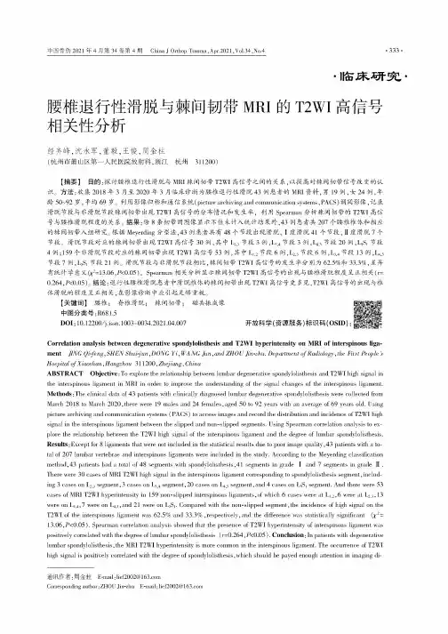
•临床研究•腰椎退行性滑脱与棘间韧带MRI的T2WI高信号相关性分析经齐峰，沈水军，董毅，王俊，周金柱(杭州市萧山区第一人民医院放射科，浙江杭州311200)【摘要】目的:探讨腰椎退行性滑脱与MRI棘间韧带T2WI高信号之间的关系，以提高对棘间韧带信号改变的认识。

方法：收集2018年3月至2020年3月临床诊断为腰椎退行性滑脱43例患者的MRI资料，男19例，女24例，年龄50~92岁，平均69岁。

利用影像归档和通信系统(picturearchivingandcommunicationsystems,PACS)调阅影像，记录滑脱节段与非滑脱节段棘间韧带出现T2WI高信号的分布情况和发生率，利用Spearman分析棘间韧带的T2WI高信号与腰椎滑脱程度的关系。

结果：除8条韧带因图像显示不佳未计入统计结果外，43例患者共207个腰椎椎体和相应的棘间韧带入组研究。

根据Meyerding分型法,43例患者共有48个节段出现滑脱，I度滑脱41个节段，域度滑脱7个节段。

滑脱节段对应的棘间韧带出现T2WI高信号30例，其中L2.3节段3例，L3.4节段3例，蕴4,5节段20例丄5S］节段4例；159个非滑脱节段对应的棘间韧带出现T2WI高信号53例，其中L,.2节段6例，L?」节段6例，L s,*节段13例,L4.5节段7例丄5S］节段21例。

滑脱节段与非滑脱节段相比，棘间韧带T2WI高信号的发生率分别为62.5%和33.3%,差异有统计学意义(v2=13.06,P<0.05)遥Spearman相关分析显示棘间韧带T2WI高信号的出现与腰椎滑脱程度呈正相关(r=0.264,P<0.05)遥结论:退行性腰椎滑脱患者中滑脱椎体的棘间韧带出现T2WI高信号更多见,T2WI高信号的出现与椎体滑脱的程度呈正相关，在影像诊断中应引起足够重视。

【关键词】腰椎；脊椎滑脱；棘间韧带；磁共振成像./.中图分类号:R681.5DOI：10.12200/j.issn.l003-0034.2021.04.007开放科学(资源服务)标识码(OSID)：.Correlation analysis between degenerative spondylolisthesis and T2WI hyperintensity on MRI of interspinous liga­ment JING匝i7/eng,S匀耘晕S澡怎円怎n,D0晕G再i,宰粤晕G允怎n,and在匀韵哉Jin-z澡怎.Department ofRadiology, the First Aop/e H匀ospita造o枣Xiaoshan，匀angzho怎311200,Zhej iang,ChinaABSTRACT Objective：To explore the relationship between lumbar degenerative spondylolisthesis and T2WI high signal inthe interspinous ligament in MRI in order to improve the understanding of the signal changes of the interspinous ligament. Methods：The clinical data of43patients with clinically diagnosed lumbar degenerative spondylolisthesis were collected fromMarch2018to March2020,there were19males and24females,aged50to92years with an average of69years ingpicture archiving and communication systems(PACS)to access images and record the distribution and incidence of T2WI highsignal in the interspinous ligament between the slipped and non・slipped ing Spearman correlation analysis to ex­plore the relationship between the T2WI high signal of the interspinous ligament and the degree of lumbar spondylolisthesis. Results:Except for8ligaments that were not included in the statistical results due to poor image quality,43patients with a to­tal of207lumbar vertebrae and interspinous ligaments were included in the study.According to the Meyerding classification method,43patients had a total of48segments with spondylolisthesis,41segments in grade I and7segments in grade域.There were30cases of MRI T2WI high signal in the interspinous ligament corresponding to spondylolisthesis segment,includ­ing3cases on L2,3segment,3cases on L3,4segment,20cases on L4,5segment,and4cases on L5S1segment.And there were53cases of MRI T2WI hyperintensity in159non-slipped interspinous ligaments,of which6cases were at L,2,6were at L2,3,13were on L3,4,7were on L4,5,and21were on pared with the non-slipped segment,the incidence of high signal on theT2WI of the interspinous ligament was62.5%and33.3%,respectively,and the difference was statistically significant(2=13.06,P<0.05).Spearman correlation analysis showed that the presence of T2WI hyperintensity of interspinous ligament was positively correlated with the degree of lumbar spondylolisthesis(r=0.264,P<0.05).Conclusion:In patients with degenerativelumbar spondylolisthesis,the MRI T2WI hyperintensity is more common in the interspinous ligament.The occurrence of T2WIhigh signal is positively correlated with the degree of spondylolisthesis,which should be payed enough attention in imaging di-通讯作者:周金柱E-mail：****************Corresponding author：ZHOU Jin-zhu E-mail:****************agnosis.KEYWORDS Lumber vfftfbfef ； Spondylolysis ； Interspinous ligament ； Magnetic ffsonenff imaging腰椎退行性滑脱（lumbardegenerative spondy ­lolisthesis ,LDS ）是由于腰椎退行性变引起的相邻椎 体间的位置滑移,LDS 是导致中老年人下腰痛的一 个重要原因。

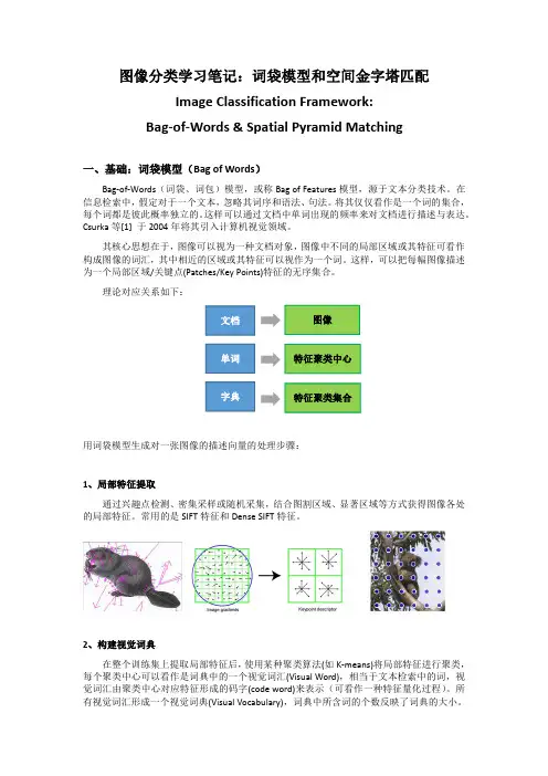
图像分类学习笔记：词袋模型和空间金字塔匹配Image Classification Framework:Bag-of-Words&Spatial Pyramid Matching一、基础：词袋模型（Bag of Words）Bag-of-Words（词袋、词包）模型，或称Bag of Features模型，源于文本分类技术。

在信息检索中，假定对于一个文本，忽略其词序和语法、句法。

将其仅仅看作是一个词的集合，每个词都是彼此概率独立的。

这样可以通过文档中单词出现的频率来对文档进行描述与表达。

Csurka等[1]于2004年将其引入计算机视觉领域。

其核心思想在于，图像可以视为一种文档对象，图像中不同的局部区域或其特征可看作构成图像的词汇，其中相近的区域或其特征可以视作为一个词。

这样，可以把每幅图像描述为一个局部区域/关键点(Patches/Key Points)特征的无序集合。

理论对应关系如下：图像特征聚类中心特征聚类集合用词袋模型生成对一张图像的描述向量的处理步骤：1、局部特征提取通过兴趣点检测、密集采样或随机采集，结合图割区域、显著区域等方式获得图像各处的局部特征。

常用的是SIFT特征和Dense SIFT特征。

2、构建视觉词典在整个训练集上提取局部特征后，使用某种聚类算法(如K-means)将局部特征进行聚类，每个聚类中心可以看作是词典中的一个视觉词汇(Visual Word)，相当于文本检索中的词，视觉词汇由聚类中心对应特征形成的码字(code word)来表示（可看作一种特征量化过程）。

所有视觉词汇形成一个视觉词典(Visual Vocabulary)，词典中所含词的个数反映了词典的大小。

3、特征量化编码图像中的每个特征都将被映射到视觉词典的某个词上，然后统计每个视觉词在一张图像上的出现次数，即可将该图像描述为一个维数固定的直方图向量。

4、训练分类模型并预测用于图像分类时，如上对训练集提取Bag-of-Features特征，在某种监督学习（如SVM）的策略下，对训练集的Bag-of-Features特征向量进行训练，获得对象或场景的分类模型；在分类模型下，对该特征进行预测，从而实现对待测图像的分类。

基于Fisher的线性判别回归分类算法曾贤灏;石全民【摘要】To improve the robustness of the linear regression classification (LRC) algorithm, a linear discrimi⁃nant regression classification algorithm based on Fisher criterion is proposed. The ratio of the between-classre⁃construction error over the within-class reconstruction error is maximized by Fisher criterion so as to find an opti⁃mal projection matrixfor the LRC. Then, all testing and training images are projected to each subspace by the op⁃timal projection matrix and Euclidean distances between testing image and all training images are computed. Fi⁃nally, K-nearest neighbor classifier is used to finish face recognition . Experimental results on AR face databases show that proposed method has better recognition effects than several other regression classification approaches.%为了提高线性回归分类（LRC）算法的鲁棒性，提出了一种基于Fisher准则的线性判别回归分类算法。

Color image segmentation using histogram thresholding –Fuzzy C-means hybrid approachKhang Siang Tan,Nor Ashidi Mat Isa nImaging and Intelligent Systems Research Team (ISRT),School of Electrical and Electronic Engineering,Engineering Campus,Universiti Sains Malaysia,14300Nibong Tebal,Penang,Malaysiaa r t i c l e i n f oArticle history:Received 29March 2010Received in revised form 2July 2010Accepted 4July 2010Keywords:Color image segmentation Histogram thresholding Fuzzy C-meansa b s t r a c tThis paper presents a novel histogram thresholding –fuzzy C-means hybrid (HTFCM)approach that could find different application in pattern recognition as well as in computer vision,particularly in color image segmentation.The proposed approach applies the histogram thresholding technique to obtain all possible uniform regions in the color image.Then,the Fuzzy C-means (FCM)algorithm is utilized to improve the compactness of the clusters forming these uniform regions.Experimental results have demonstrated that the low complexity of the proposed HTFCM approach could obtain better cluster quality and segmentation results than other segmentation approaches that employing ant colony algorithm.&2010Elsevier Ltd.All rights reserved.1.IntroductionColor is one of the most significant low-level features that can be used to extract homogeneous regions that are most of the time related to objects or part of objects [1–3].In a 24-bit true color image,the number of unique colors usually exceeds half of the image size and can reach up to 16millions.Most of these colors are perceptually close and cannot be differentiated by human eye that can only internally identify a number of 30colors in cognitive space [4,5].For all unique colors that perceptually close,they can be combined to form homogeneous regions representing the objects in the image and thus,the image could become more meaningful and easier to be analyzed.In image processing and computer vision,color image segmentation is a central task for image analysis and pattern recognition [6–23]It is a process of partitioning an image into multiple regions that are homogeneous with respect to one or more characteristics.Although many segmentation techniques have been appeared in scientific literature,they can be divided into image-domain based,physics based and feature-space based techniques [24].These segmentation techniques have been used extensively but each has its own advantages and limitations.Image-domain based techniques utilize both color features and spatial relationship among color in its homogeneity evaluation to perform segmenta-tion.These techniques produce the regions that have reasonablecompactness of regions but facing difficulty in the selection of suitable seed regions.Physics based techniques utilize the physical models of the reflection properties of material to carry out color segmentation but more application specific,as they model the causes that may produce color variation.Feature-based techniques utilize color features as the key and the only criteria to segment image.The segmented regions are usually fragmented since the spatial relationship among color is ignored [25].But this limitation can be solved by improving the compactness of the regions.In computer vision and pattern recognition,Fuzzy C-means (FCM)algorithm has been used extensively to improve the compactness of the regions due to its clustering validity and simplicity of implementation.It is a pixels clustering process of dividing pixels into clusters so that pixels in the same cluster are as similar as possible and those in different clusters are as dissimilar as possible.This accords with segmentation application since different regions should be visually as different as possible.However,its implementation often encounters two unavoidable initialization difficulties of deciding the cluster number and obtaining the initial cluster centroids that are properly distrib-uted.These initialization difficulties have their impacts on segmentation quality.While the difficulty of deciding the cluster number could affect the segmented area and region tolerance for feature variance,the difficulty of obtaining the initial cluster centroids could affect the cluster compactness and classification accuracy.Recently,some feature-based segmentation techniques have employed the concept of ant colony algorithm (ACA)to carry out image segmentation.Due to the intelligent searching ability of theContents lists available at ScienceDirectjournal homepage:/locate/prPattern Recognition0031-3203/$-see front matter &2010Elsevier Ltd.All rights reserved.doi:10.1016/j.patcog.2010.07.013nCorresponding author.Tel.:+6045996093;fax:+6045941023.E-mail addresses:khangsiang85@ (K.Siang Tan),ashidi@m.my (N.A.Mat Isa).Pattern Recognition 44(2011)1–15ACA,these techniques could achieve further optimization of segmentation results.But they are suffering from low efficiency due to their computational complexity.Apart from obtaining good segmentation result,the improved ant system algorithm(AS)as proposed in[26]could also provide a solution to overcome the FCM’s sensitiveness to the initialization condition of cluster centroids and centroid number.However,the AS technique does not seek for very compact clustering result in the feature space.To improve the performance of the AS,the ant colony–Fuzzy C-means hybrid algorithm(AFHA)is introduced[26].Essentially, the AFHA incorporates the FCM algorithm to the AS in order to improve the compactness of the clustering results in the feature space.However,its efficiency is still low due to computational complexity of the AS.To increase the algorithmic efficiency of the AFHA,the improved ant colony–Fuzzy C-means hybrid algorithm (IAFHA)is introduced[26].The IAFHA adds an ant sub-sampling based method to modify the AFHA in order to reduce its computational complexity thus has higher efficiency.Although the IAFHA’s efficiency has been increased,it still suffers from high computational complexity.In this paper,we propose a novel segmentation approach called Histogram Thresholding–Fuzzy C-means Hybrid(HTFCM) algorithm.The HTFCM consists of two modules,namely the histogram thresholding module and the FCM module.The histogram thresholding module is used for obtaining the FCM’s initialization condition of cluster centroids and centroid number. The implementation of this module does not require high computational complexity comparing to those techniques using ant system.This marked the simplicity of the proposed algorithm.The rest of the paper is organized as follows:Section2 presents the histogram thresholding module and the FCM module in detail.Section3provides the illustration of the implementation procedure.Section4analyzes the result obtained for the proposed approach and at the same time comparing it to other techniques. Finally,Section5concludes the work of this paper.2.Proposed approachIn this paper,we attempt to obtain a solution to overcome the FCM’s sensitiveness to the initialization conditions of cluster centroid and centroid number.The histogram thresholding module is introduced to initialize the FCM in view of the drawbacks by taking the global information of the image into consideration.In this module,the global information of the image is used to obtain all possible uniform regions in the image and thus the cluster centroids and centroid number could also be obtained.The FCM module is then used to improve the compactness of the clusters.In this context,the compactness refers to obtaining the optimized label for each cluster centroid from the members of each cluster.2.1.Histogram thresholdingGlobal histogram of a digital image is a popular tool for real-time image processing due to its simplicity in implementation.It serves as an important basis of statistical approaches in image processing by producing the global description of the image’s information[27].For color images with RGB representation,the color of a pixel is a mixture of the three primitive colors red,green and blue.Each image pixel can be viewed as three dimensional vector containing three components representing the three colors of an image pixel.Hence,the global histograms representing three primitive components,respectively,could produce the global information about the entire image.The basic analysis approach of global histogram is that a uniform region tends to form a dominating peak in the corresponding histogram.For a color image,a uniform region could be identified by the dominating peaks in the global histograms.Thus,histogram thresholding is a popular segmenta-tion technique that looks for the peaks and valleys in histogram [28,29].A typical segmentation approach based on histogram analysis can only be carried out if the dominating peaks in the histogram can be recognized correctly.Several widely used peak-finding algorithms examined the peak’s sharpness or area to identify the dominating peaks in the histogram.Although these peak-finding algorithms are useful in histogram analysis,they sometimes do not work well especially if the image contains noise or radical variation[30,31].In this paper,we propose a novel histogram thresholding technique containing three phases such as the peakfinding technique,the region initialization and the merging process.The histogram thresholding technique applies a peakfinding techni-que to identify the dominating peaks in the global histograms.The peakfinding algorithm could locate all the dominating peaks in the global histograms correctly and have been proven to be efficient by testing on numerous color images.As a result,the uniform regions in the image could be obtained.Since any uniform region contains3components representing the3colors of the RGB color image,each component of the uniform region is assigned one value corresponding to the intensity level of one dominating peak in their respective global histograms.Although the uniform regions are successfully obtained,some uniform regions are still perceptually close.Thus,a merging process is applied to merge these regions together.2.1.1.PeakfindingLet us suppose dealing with color image with RGB representa-tion which each of the primitive color components’intensity is stored in n-bit integer,giving a possible L¼2n intensity levels in the interval[0,LÀ1].Let r(i),g(i)and b(i)be the red component, the green component and the blue component histograms, respectively.Let x i,y i and z i be the number of pixels associated with i th intensity level in r(i),g(i)and b(i),respectively.The peakfinding algorithm can be described as follows:i.Represent the red component,green component and bluecomponent histograms by the following equations:rðiÞ¼x i,ð1ÞgðiÞ¼y i,ð2ÞbðiÞ¼z i,ð3Þwhere0r i r LÀ1.ii.From the original histogram,construct a new histogram curve with the following equation:T sðiÞ¼ðsðiÀ2ÞþsðiÀ1ÞþsðiÞþsðiþ1Þþsðiþ2ÞÞ5,ð4Þwhere s can be substituted by r,g and b and2r i r LÀ3.T r(i), T g(i)and T b(i)are the new histogram curves constructed from the red component,green component and blue component histograms,respectively.(Note:Based on analysis done using numerous images,the half window size can be set from2to5in this study.The half window size that is smaller than2could not produce a smooth histogram curve while large half window size could produce different general shape of a smooth histogram curve when comparing it to the original histogram.)K.Siang Tan,N.A.Mat Isa/Pattern Recognition44(2011)1–15 2iii.Identify all peaks using the following equation:P s¼ðði,T sðiÞÞ9T sðiÞ4T sðiÀ1Þand T sðiÞ4T sðiþ1ÞÞ,ð5Þwhere s can be substituted by r,g and b and1r i r LÀ2.P r,P g and P b are the set of peaks identified from T r(i),T g(i)and T b(i), respectively.iv.Identify all valleys using the following equation:V s¼ðði,T sðiÞÞ9T sðiÞo T sðiÀ1Þand T sðiÞo T sðiþ1ÞÞ,ð6Þwhere s can be substituted by r,g and b and1r i r LÀ2.V r,V g and V b are the set of valleys identified from T r(i),T g(i)and T b(i), respectively.v.Remove all peaks and valleys based on the following fuzzy rule base:IFði is peakÞANDðT sðiþ1Þ4T sðiÀ1ÞÞTHENðT sðiÞ¼T sðiþ1ÞÞIFði is peakÞANDðT sðiþ1Þo T sðiÀ1ÞÞTHENðT sðiÞ¼T sðiÀ1ÞÞIFði is valleyÞANDðT sðiþ1Þ4T sðiÀ1ÞÞTHENðT sðiÞ¼T sðiÀ1ÞÞIFði is valleyÞANDðT sðiþ1Þo T sðiÀ1ÞÞTHENðT sðiÞ¼T sðiþ1ÞÞ,ð7Þwhere s can be substituted by r,g and b and1r i r LÀ2.vi.Identify the dominating peaks in T r(i),T g(i)and T b(i)by examining the turning point which having positive to negative gradient change and the number of pixels is greater than a predefined threshold,H.(Note:Based on analysis done using numerous images,the typical value for H is set to20.)2.1.2.Region initializationAfter the peakfinding algorithm,three sets of dominating peak’s intensity level in the red,green and blue component histograms,respectively,are obtained.Let x,y and z be the number of dominating peaks identified in the red component, green component and blue component histograms,respectively. Then P r¼(i1,i2,y,i x),P g¼(i1,i2,y,i y)and P b¼(i1,i2,y,i z) are the sets of dominating peak’s intensity levels in the red component,green component and blue component histo-grams,respectively.A uniform region labeling by a cluster centroid tends to form one dominating peak in the red, green and blue component histograms,respectively.In this paper,the region initialization algorithm can be described as follows:i.Form all the possible cluster centroids(Note:Each componentof the cluster centroids can only take the intensity level of one dominating peak in the red,green and blue histogram, respectively.Thus,a number of(xÂyÂz)possible cluster centroids are formed.)ii.Assign every image pixels to the nearest cluster centroid and form the pixel set of each cluster by assigning them to their corresponding cluster centroid.iii.Eliminate all cluster centroids that having the number of pixels assigned to them is less than a threshold,V.(Note:To reduce the initial cluster centroid number,the value for V is set to0.006NÀ0.008N where N is the total number of pixels in that image.)iv.Reassign every image pixels to the nearest cluster centroid.(Note:Let c l be the l th element in the cluster centroid set and X l be the pixel set that are assigned to c l.)v.Update each cluster centroid,c l by the mode of its pixel set,X l, respectively.2.1.3.MergingAfter the region initialization algorithm,the uniform regions labeling by their respective cluster centroids are obtained.Some of these regions are perceptually close and could be merged together in order to produce a more concise set of cluster centroids representing the uniform region.Thus,a merging algorithm is needed to merge these regions based on their color similarity.One of the simplest measures of color similarity is the Euclidean distance which is used to measure the color difference between two uniform regions.Let C¼(c1,c2,y,c M)be the set of cluster centroids and M be the number of cluster centroids.In this paper,the merging algorithm can be described as follows:i.Set the maximum threshold of Euclidean distance,dc to apositive integer value.ii.Calculate the distance,D for any two out of these M cluster centroids with the following equation:D c j,c kÀÁ¼ffiffiffiffiffiffiffiffiffiffiffiffiffiffiffiffiffiffiffiffiffiffiffiffiffiffiffiffiffiffiffiffiffiffiffiffiffiffiffiffiffiffiffiffiffiffiffiffiffiffiffiffiffiffiffiffiffiffiffiffiffiffiffiffiffiðR jÀR kÞ2þðG jÀG kÞ2þðB jÀB kÞ2q,8j a k,ð8Þwhere1r j r M and1r k r M.R j,G j and B j are the value of the red,green and blue component of the j th cluster centroid, respectively,and R k,G k and B k are the value of the red,green and blue component of the k th cluster centroid,respectively. iii.Find the minimum distance between two nearest cluster centroids.Merge these nearest cluster centroids to form the new cluster centroid if the minimum distance between them is less than dc.Otherwise,stop the merging process.iv.Update the pixel set that assigned to the new cluster centroid by merging the pixel sets that assigned to these nearest cluster centroids.v.Refresh the new cluster centroid by the mode of its pixel set. vi.Reduce the number of cluster centroids,M to(MÀ1)and repeat steps ii to vi until no minimum distance between two nearest cluster centroids is less than dc.(Note:Based on analysis done using numerous images,the number of cluster centroids remain constant for most of the images by varying dc from24to32.)2.2.Fuzzy C-meansThe FCM algorithm is essentially a Hill-Climbing technique which was developed by Dunn in1973[32]and improved by Bezdek in1981[33].This algorithm has been used as one of the popular clustering techniques for image segmentation in compu-ter vision and pattern recognition.In the FCM,each image pixels having certain membership degree associated with each cluster centroids.These membership degrees having values in the range [0,1]and indicate the strength of the association between that image pixel and a particular cluster centroid.The FCM algorithm attempts to partition every image pixels into a collection of the M fuzzy cluster centroids with respect to some given criterion[34].Let N be the total number of pixels in that image and m be the exponential weight of membership degree.The objective function W m of the FCM is defined asW mðU,CÞ¼X Ni¼1X Mj¼1u mjid2ji,ð9Þwhere u ji is the membership degree of i th pixel to j th cluster centroid and d ji is the distance between i th pixel and j th cluster centroid.Let U i¼(u1i,u2i,y,u Mi)T is the set of membership degree of i th pixel associated with each cluster centroids,x i is the i th pixel in the image and c j is the j th cluster centroid.Then U¼(U1, U2,y,U N)is the membership degree matrix and C¼(c1,c2,y,c M) is the set of cluster centroids.K.Siang Tan,N.A.Mat Isa/Pattern Recognition44(2011)1–153The degree of compactness and uniformity of the cluster centroids greatly depend on the objective function of the FCM.In general,a smaller objective function of the FCM indicates a more compact and uniform cluster centroid set.However,there is no close form solution to produce minimization of the objective function.To achieve the optimization of the objective function,an iteration process must be carried out by the FCM algorithm.In this paper,the FCM is employed to improve the compactness of the clusters produced by the histogram thresholding module.The FCM can be described as follows:i.Set the iteration terminating threshold,e to a small positive number in the range [0,1]and the number of iteration q to 0.ii.Calculate U (q )according to C (q )with the following equation:u ji ¼1P Mk ¼1ðd ji =d ki Þ2=ðm À1Þ,ð10Þwhere 1r j r M and 1r i r N .Notice that if d ji ¼0,then u ji ¼1and set others membership degrees of this pixel to 0.iii.Calculate C (q +1)according to U (q )with the following equation:c j ¼P Ni ¼1u mji x iP i ¼1u m ji ,ð11Þwhere 1r j r M .iv.Update U (q +1)according to C (q +1)with Eq.(10).pare U (q +1)with U (q ).If :U (q +1)ÀU (q ):r e ,stop iteration.Otherwise,q ¼q +1,and repeat steps ii to iv until :U (q +1)ÀU (q ):4e .3.Illustration of the implementation procedureIn this section,we apply the HTFCM approach to perform the segmentation with the 256Â256image House depicted in Fig.1(a).Figs.2(a),3(a)and 4(a)show the red,green and blue component histogram of the image,respectively.In Fig.2(a),the dominating peaks that could represent the red component of dominant regions are difficult to be recognized as a large number of small peaks exist in the histogram.The similar case has also been shown in Figs.3(a)and 4(a).These small peaks must be removed so that the dominating peaks can be recognized effectively.Thus,the dominating peaks are recognized according to the proposed peak finding technique.Figs.2(b),3(b)and 4(b)show the resultant histogram curves,after applying the proposed peak finding technique.Since the general shape of each resultant histogram curve have a great similarity with their respective original histogram,the dominating peak in the histogram curve can be considered as the dominating peak in their respective histogram.Furthermore,each of the resultant histogram curves gives better degree of smoothness than their respective original histogram.As a result,the dominating peaks in the histogram canbe recognized easily by examining the histogram curve.Then,the initial clusters are formed by assigning every pixel to their cluster centroids,respectively.For example,the left uppermost pixel in the image having the RGB value of (159,197,222)is assigned to the centroid having the RGB value of (159,199,224)since the Euclidean distance between the pixel and the centroid is the shortest compared to other centroids.The RGB valueofFig.1.Image House and its segmentation results.(a)Original image House ,(b)image after cluster centroid initialization,(c)image after merging and (d)final segmentationresult.Fig.2.(a)Red component histogram of image House ,(b)resultant histogram curve after peak finding technique (Note:The intensity level of the dominating peaks is labeled by x ).K.Siang Tan,N.A.Mat Isa /Pattern Recognition 44(2011)1–154the centroid is obtained from one of the dominating peaks in Figs.2(b),3(b)and 4(b),respectively.The result of initial clusters is illustrated in Fig.1(b).Next,the merging process is carried out to merge all the clusters that are perceptually close.This merging process is able to reduce the cluster number and keep a reasonable cluster number for all kinds of input images.The result of the merging process is illustrated in Fig.1(c).Finally,the FCM algorithm is applied to perform color segmentation.The final segmentation result is illustrated in Fig.1(d).4.Experiment resultsThe HTFCM approach has been tested on more than 200images taken from public image segmentation databases.In this paper,30images are selected to demonstrate the capability of the proposed HTFCM approach.8out of these images namely House (256Â256),Football (256Â256),Golden Gate (256Â256),Smarties (256Â256),Capsicum (256Â256),Gantry Crane (400Â264),Beach (321Â481)and Girl (321Â481)are evaluated in details to highlight the advantages of the proposed HTFCM approach.While another 22images are presented as supplementary images to further support the findings.The AS,the AFHA and the IAFHA approaches which are proved to be able to provide good solution to overcome the FCM’s sensitiveness to the initialization condi-tions of cluster centroids and centroid number are used as comparison in order to see whether the HTFCM approach could result in generally better performance and cluster quality than these approaches.The performance of the HTFCM approach is evaluated by comparing the algorithmic efficiency and the segmentation results with the AS,the AFHA and the IAFHA approaches.In this study,we fix dc as 28since it tend to produce reasonable results for the AS,the AFHA,the IAFHA [26]and the HTFCM approaches.4.1.Evaluation on segmentation resultsIn this section,the segmentation results for the AS,the AFHA,the IAFHA and the HTFCM approaches are evaluated visually.Generally,as shown in Figs.5–12,the proposed HTFCM approach produces better segmentation results as compared to the AS,theFig.3.(a)Green component histogram of image House and (b)resultant histogram curve after peak finding technique (Note:The intensity level of the dominating peaks is labeled by x.).Fig.4.(a)Blue component histogram of image House and (b)resultant histogram curve after peak finding technique (Note:The intensity level of the dominating peaks is labeled by x .).K.Siang Tan,N.A.Mat Isa /Pattern Recognition 44(2011)1–155AFHA and the IAFHA approaches.The segmented regions of the resultant images produced by the HTFCM approach are more homogeneous.For example,notice for the image House ,the HTFCM approach gives better segmentation result than the AS,the AFHA and the IAFHA approaches by producing more homogeneous house roof and walls as depicted in Fig.5.In the image Football ,the HTFCM approach also outperforms the AS,the AFHA and the IAFHA approaches by giving more homogeneous background as shown in Fig.6.As for the image Golden Gate ,although the AS,the AFHA and the IAFHA approaches produce homogeneous sky region,but an obvious classification error could be seen where these approaches mistakenly assign considerable pixels of the leave of tree as part of the bridge.The proposed HTFCM approach successfully avoids this classification error and furthermore,produces more homogeneous hill and sea regions as shown in Fig.7.In the image Capsicum ,the proposedHTFCMFig.5.The image House :(a)original image,and the rest are segmentation results of the test image by various algorithms (b)AS,(c)AFHA,(d)IAFHA,and (e)HTFCM.Fig.6.The image Football :(a)original image,and the rest are segmentation results of the test image by various algorithms (b)AS,(c)AFHA,(d)IAFHA,and (e)HTFCM.K.Siang Tan,N.A.Mat Isa /Pattern Recognition 44(2011)1–156approach also outperforms other techniques by producing more homogeneous red capsicum as depicted in Fig.8.Notice for the image Smarties ,the AS,the AFHA and the IAFHA approaches mistakenly assign considerable pixels of the background as part of the green Smarties.The proposed HTFCM approach successfully avoids this classification error and furthermore,produces more homogeneous background as shown in Fig.9.As for the image Beach ,the HTFCM approach outperforms others approaches by giving more homogeneous beach and sea as depicted in Fig.10.As for the image Gantry Crane ,there is a classification error where part of the left-inclined truss has been assigned to the sky by the AS,the AFHA and the IAFHA approaches as shown in Fig.11.The proposed HTFCM successfully avoids this classification error.The similar result is obtained for the image Girl .The HTFCM approach outperforms other approaches by classifying the blue and red part of the shirt as single cluster while theAS,Fig.7.The image Golden Gate :(a)original image,and the rest are segmentation results of the test image by various algorithms (b)AS,(c)AFHA,(d)IAFHA,and (e)HTFCM.Fig.8.The image Capsicum :(a)original image,and the rest are segmentation results of the test image by various algorithms (b)AS,(c)AFHA,(d)IAFHA,and (e)HTFCM.K.Siang Tan,N.A.Mat Isa /Pattern Recognition 44(2011)1–157Fig.9.The image Smarties :(a)original image,and the rest are segmentation results of the test image by various algorithms (b)AS,(c)AFHA,(d)IAFHA,and (e)HTFCM.Fig.10.The image Beach :(a)original image,and the rest are segmentation results of the test image by various algorithms (b)AS,(c)AFHA,(d)IAFHA,and (e)HTFCM.K.Siang Tan,N.A.Mat Isa /Pattern Recognition 44(2011)1–158。

Phase-Based User-Steered Image Segmentation Lauren O’Donnell1,Carl-Fredrik Westin1,2,W.Eric L.Grimson1, Juan Ruiz-Alzola3,Martha E.Shenton2,and Ron Kikinis21MIT AI Laboratory,Cambridge MA02139,USAodonnell,***********.edu2Brigham and Women’s Hospital,Harvard Medical School,Boston MA,USAwestin,*******************.edu3Dept.of Signals and Communications,University of Las Palmas de Gran Canaria,Spain***************.esAbstract.This paper presents a user-steered segmentation algorithmbased on the livewire paradigm.Livewire is an image-feature drivenmethod thatfinds the optimal path between user-selected image loca-tions,thus reducing the need to manually define the complete boundary.We introduce an image feature based on local phase,which describes lo-cal edge symmetry independent of absolute gray value.Because phase isamplitude invariant,the measurements are robust with respect to smoothvariations,such as biasfield inhomogeneities present in all MR images.Inorder to enable validation of our segmentation method,we have createda system that continuously records user interaction and automaticallygenerates a database containing the number of user interactions,such asmouse events,and time stamps from various editing modules.We haveconducted validation trials of the system and obtained expert opinionsregarding its functionality.1IntroductionMedical image segmentation is the process of assigning labels to voxels in order to indicate tissue type or anatomical structure.This labeled data has a variety of applications,for example the quantification of anatomical volume and shape,or the construction of detailed three-dimensional models of the anatomy of interest.Existing segmentation methods range from manual,to semi-automatic,to fully automatic.Automatic algorithms include intensity-based methods,such as EM segmentation[14]and level-sets[4],as well as knowledge-based methods such as segmentation by warping to an anatomical atlas.Semi-automatic algorithms, which require user interaction during the process,include snakes[11]and livewire [1,7].Current practice in many cases,however,is computer-enhanced manual segmentation.This involves hand-tracing around the structures of interest and perhaps employing morphological or thresholding operations to the data.Although manual segmentation methods allow the highest degree of user control and enable decisions to be made on the basis of extensive anatomical knowledge,they require excessive amounts of user interaction time and mayW.Niessen and M.Viergever(Eds.):MICCAI2001,LNCS2208,pp.1022–1030,2001.c Springer-Verlag Berlin Heidelberg2001Phase-Based User-Steered Image Segmentation1023 introduce high levels of variability.On the other hand,fully automatic algorithms may not produce the correct outcome every time,hence there exists a need for hybrid methods.2Existing Software PlatformThe phase-based livewire segmentation method has been integrated into the 3D Slicer,the Surgical Planning Lab’s platform for image visualization,image segmentation,and surgical guidance[9].The Slicer is the laboratory’s program of choice for manual segmentation,as well as being modular and extensible,and consequently it is the logical place to incorporate new algorithms for our user base.At any time during an average day,one would expect tofind ten people doing segmentations using the3D Slicer in the laboratory,which shows that any improvement on manual methods will be of great utility.Our system has been added into the Slicer as a new module,Phasewire,in the Image Editor.3The Livewire AlgorithmThe motivation behind the livewire algorithm is to provide the user with full control over the segmentation while having the computer do most of the detail work[1].In this way,user interaction complements the ability of the computer tofind boundaries of structures in an image.Initially when using this method,the user clicks to indicate a starting point on the desired contour,and then as the mouse is moved it pulls a“live wire”behind it along the contour.When the user clicks again,the old wire freezes on the contour,and a new live one starts from the clicked point.This intuitive method is driven only by image information,with little geometric constraint,so extracting knowledge from the image is of primary importance.The livewire method poses this problem as a search for shortest paths on a weighted graph.Thus the livewire algorithm has two main parts,first the conversion of image information into a weighted graph,and then the calculation of shortest paths in the graph[6,12].In thefirst part of the livewire algorithm,weights are calculated for each edge in the weighted graph,creating the image forces that attract the livewire. To produce the weights,various image features are computed in a neighborhood around eachgraphedge,transformed to give low edge costs to more desirable feature values,and then combined in some user-adjustable fashion.The general purpose of the combination is edge localization,but individual features are gen-erally chosen for their contributions in three main areas,which we will call“edge detection,”“directionality,”and“training.”Features suchas th e gradient and the Laplacian zero-crossing[13]have been used for edge detection;these features are the main attractors for the livewire.Second,directionality,or the direction the path should take locally,can be influenced by gradients computed with ori-ented kernels[7],or the“gradient direction”feature[13].Third,training is the1024L.O’Donnell et al.process by which the user indicates a preference for a certain type of bound-ary,and the image features are transformed accordingly.Image gradients and intensity values[7],as well as gradient magnitudes[13],are useful in training.In the second part of the livewire algorithm,Dijkstra’s algorithm[5]is used to find all shortest paths extending outward from the starting point in the weighted graph.The livewire is defined as the shortest path that connects two user-selected points(the last clicked point and the current mouse location).This second step is done interactively so the user may view and judge potential paths,and con-trol the segmentation asfinely as desired.The implementation for this paper is similar to that in[6],where the shortest paths are computed for only as much of the image as necessary,making for very quick user interaction.4Phase-Based Livewire4.1Background on Local PhaseThe local phase as discussed in this paper is a multidimensional generalization of the concept of instantaneous phase,which is formally defined as the argument of the analytic functionf A=f−if Hi(1) where f Hi denotes the Hilbert transform of f[2,3].The instantaneous phase of a simple one-dimensional signal is shown in Fig-ure1.This simple signal can be thought of as the intensity along a row of pixels in an image.Note that in this“image”there are two edges,or regions where the signal shape is locally odd,and the phase curve reacts to each,giving phase values ofπ/2and−π/2.Fig.1.AThe output from a local phasefilter,i.e.a Gaborfilter,is an analytic function that can be represented as an even real part and an odd imaginary part,or anPhase-Based User-Steered Image Segmentation1025 amplitude and an argument.Consequently,this type offilter can be used to estimate both the amplitude(energy)and the local phase of a signal.As local phase is invariant to signal energy,edges can be detected from small or large signal variations.This is advantageous for segmentation along weak as well as strong edges.Another advantage is that local phase is in general a smoothly varying function of the image,and provides subpixel information about edge position.4.2ImplementationTo estimate the phase we are using quadraturefilters which have a radial fre-quency function that is Gaussian on a logarithmic scale:ν(ρ)=e−4log2B−2log2(ρρi)(2) whereρi is the center frequency and B is the6dB sensitivity bandwidth in octaves.In contrast to Gaborfilters,thesefilters have zero response for negative frequencies,ensuring that the odd and even parts constitute a Hilbert transform pair and making thefilters ideal for estimation of local phase[10].We multiply thefilters with a cos2radial function window in the frequency domain to reduce ringing artifacts arising from the discontinuity atπwhen usingfilters with high center frequencies and/or large bandwidth.The local phase is our primary feature,serving to localize edges in the image: the livewire essentially follows along low-cost curves in the phase image.The phase feature is scaled to provide bounded input to the shortest-paths search. Figure2shows a phase image derived from the original image shown in Figure 4.Since the argument of the phase is not sensitive to the amount of energy in the signal,it is useful to also quantify the certainty of the phase estimate.In image regions where the phase magnitude is large,the energy of the signal is high,which implies that the the phase estimate in that region has high reliability and thus high certainty.We define the certainty using the magnitude from the quadraturefilters, mapped through a gating function.By inverting this certainty measure,it can be used as a second feature in the livewire cost function.The weighted combination of the phase and certainty images produces an output image that describes the edge costs in the weighted graph,as in Figure2.5ApplicationsIn this section,we describe the behavior of our phase-based segmentation tech-nique through a series of experiments with medical images.In thefirst set of experiments,we show the stability of phase information across different scales[8].The input to the quadraturefilters was blurred using a Gaussian kernel of variance4pixels.Figure3demonstrates the robustness1026L.O’Donnell et al.Local Phase Image Combined ImageFig.2.Local phase images.The left-hand image shows the local phase corre-sponding to the grayscale image in Figure 4.This is the primary feature employed in our phase-based livewire method.The right-hand image displays the weighted combination of the phase and certainty features,which emphasizes boundaries in the image.Darker pixels correspond to lower edge costs on the weighted graph.of phase information to changes in scale,as the two segmentations are quite similar.The leftmost image is the original grayscale and its segmentation,while the center image shows the result of Gaussian blurring.The rightmost image displays the segmentation curve from the blurred image over the original image for comparison.The second experiments contrast the new livewire feature,phase,with our original intensity-based livewire implementation.Phase is more intuitive to use,produces smoother output,and is generally more user-friendly than the intensity-based method as illustrated in Figure 4.In contrast to the intensity-based method,no training step is required to bias the phase-based method towards the desired edge type,as the phase information can be used to follow weak or strong edges.6Discussion and Validation FrameworkWe have presented a user-steered segmentation algorithm which is based on the livewire paradigm.Our preliminary results using local phase as the main driving force are promising and support the concept that phase is a fairly stable feature in scale space [8].The method is intuitive to use,and requires no training despite having fewer input image features than other livewire implementations.In order to enable validation of phase-based livewire,we have created a sys-tem that continuously records user interaction and can generate a database con-taining the number of user interactions and time stamps from various editing modules.A selection of the items which are recorded is listed in Table 1.AnPhase-Based User-Steered Image Segmentation1027Original Image Gaussian Blurring Overlay of SegmentationFig.3.Illustration of insensitivity to changes in scale:initial image,result of Gaussian blurring,and overlay of second segmentation(done on the blurred image)on initial image.Note the similarity between the segmentation contours, despite blurring the image with a Gaussian kernel of four pixel variance. ongoing study using this system will enable evaluation of the performance and utility of different image features for guiding the livewire.Analysis of the logged information has shown that great variability exists in segmentation times,partially due to users’segmentation style,learning curve, and type of image data,and also due to factors we cannot measure,suchas time spent using other programs with the Slicer Editor window open.A complete comparison of the phasewire and manual segmentations systems,consequently, is difficult,and perhaps the most reliable indication of the system performance can be found in the opinions of doctors who have used it.Table2demonstrates the utility of the segmentation method using infor-mation from the logging system,and Table3gives doctors’opinions regarding ease of use and quality of output segmentations.For example,Figure5shows a liver segmentation done with phasewire,in which the doctor remarked that the three-dimensional model was more anatomically accurate than the one pro-duced with the manual method,where both segmentations were performed in approximately the same amount of time.This is likely due to the smoothness of the contour obtained with phasewire,in comparison with the contour obtained with the manual method.Item Logged Detailsmouse clicks recorded per slice,per label value,per volume,and per editor module elapsed time recorded per slice,per label value,per volume,and per editor module description includes volumes viewed and location of scene descriptionfile username will allow investigation of learning curveTable1.Selected items logged by the3D Slicer for validation and comparison purposes.1028L.O’Donnell et al.parison of phase-based and intensity-based implementations of livewire.On the left is our original implementation of livewire,which uses image-intensity based features.It does a poorer job of segmenting gray and white mat-ter.Training was performed on the region in the upper left of the image.The segmentation was more difficult to perform than the phase-based segmentation because more coercing was necessary to force the livewire to take an accept-able path.The right image shows segmentation of the same boundary using the phase-based livewire.Contrary to the intensity-based method,no training was necessary before beginning to segment.The conclusion is that the phase-based implementation is more intuitive to use than the intensity-based version,since the phase image gives continuous contours for the livewire to follow.Rather than being distracted by unwanted pixels locally,the phase livewire is generally only distracted by other paths,and a small movement of the mouse can set it back on the desired path.It can be quitefluid to use,with clicks mainly necessary when the curve bends in order to keep the wire following the correct contour. 7AcknowledgementsThe work was funded in part by CIMIT and NIH P41-RR13218(RK,CFW),by a National Science Foundation G raduate ResearchFellowsh ip(LJO),by NIH R01 RR11747(RK),by Department of Veterans Affairs Merit Awards,NIH grants K02MH01110and R01MH50747(MS),and by European Commission and Spanish Gov.joint research grant1FD97-0881-C02-01(JR).Thanks to the Radi-ation Oncology,Medical Physics,Neurosurgery,Urology,and Gastroenterology Departments of Hospital Doctor Negrin in Las Palmas de Gran Canaria,Spain, for their participation in evaluation of the system.Also thanks to Aleksandra Ciszewski for her valuable feedback regarding the Slicer system. References1.W.A.Barrett and E.N.Mortensen.Interactive live-wire boundary extraction.Medical Image Analysis,1(4):331–341,1997.Phase-Based User-Steered Image Segmentation1029Fig.5.A surface model of the liver,created from a phasewire segmentation, shows well-defined surfaces between the liver and the kidney and gallbladder. study method total clicks clicks/slice time/slice(sec)volume(mL) CT brain tumor manual23426.039.368.5phasewire9710.828.767.3phasewire10912.125.569.2CT bladder manual148828.131.7715.6phasewire359 6.821.5710.8Table2.Example segmentations performed withPh asewire.Clicks and time per slice are averages over the dataset.2.Boualem Boashash.Estimating and interpreting the instantaneous frequency of asignal-part1:Fundamentals.Proceedings of the IEEE,80(4),1992.3.Boualem Boashash.Estimating and interpreting the instantaneous frequency of asignal-part2:Algorithms and applications.Proceedings of the IEEE,80(4),1992.4.V.Caselles,R.Kimmel,G.Sapiro,C.Sbert.Minimal Surfaces:A Three DimensionalSegmentation Approach.Technion EE Pub973,1995.5. E.W.Dijkstra A Note On Two Problems in Connexion With Graphs NumerischeMathematik,269–271,1959.6. A.X.Falcao,J.K.Udupa,and F.K.Miyazawa.An Ultra-Fast User-Steered ImageSegmentation Paradigm:Live Wire on the Fly.IEEE Transactions on Medical Imaging,19(1):55–61,2000.7. A.X.Falcao,J.K.Udupa,S.Samarasekera,and er-Steered ImageSegmentation Paradigms:Live Wire and Live Lane.Graphical Models and Image Processing,60:233–260,1998.8. D.J.Fleet and A.D.Jepson.Stability of Phase Information IEEE Trans.PAMI,15(12):1253–1268,1993.9. D.T.Gering,A.Nabavi,R.Kikinis,W.E.L.Grimson,N.Hata,P.Everett,andF.Jolesz and W.Wells.An Integrated Visualization System for Surgical Plan-ning and Guidance Using Image Fusion and Interventional Imaging.Medical Image Computing and Computer-Assisted Intervention-MICCAI’99,809–819,1999.1030L.O’Donnell et al.study method ease of use segmentation qualityCT brain tumor manual33phasewire44CT bladder manual 2.73phasewire44Table3.Doctors’comparison of Phasewire and Manual segmentation methods on the datasets from Table2.The scale is from1to5,with5being the highest.10.H.Knutsson and C.-F.Westin and G.H.Granlund.Local Multiscale Frequencyand Bandwidth Estimation Proceedings of IEEE International Conference on Image Processing,36–40,1994.11.T.McInerney,D.Terzopoulos.Deformable Models in Medical Image Analysis:ASurvey.Medical Image Analysis,1(2):91–108,1996.12. E.N.Mortensen and W.A.Barrett.Interactive Segmentation with IntelligentScissors.Graphical Models and Image Processing,60(5):349–384,1998.13. E.N.Mortensen and W.A.Barrett.Intelligent Scissors for Image Composition.Computer Graphics(SIGGRAPH‘95),191–198,1995.14.W.M.Wells,R.Kikinis,W.E.L.Grimson,F.Jolesz.Adaptive segmentation ofMRI data.IEEE Transactions on Medical Imaging,15:429–442,1996.。