Lecture 12
- 格式:pdf
- 大小:142.21 KB
- 文档页数:3
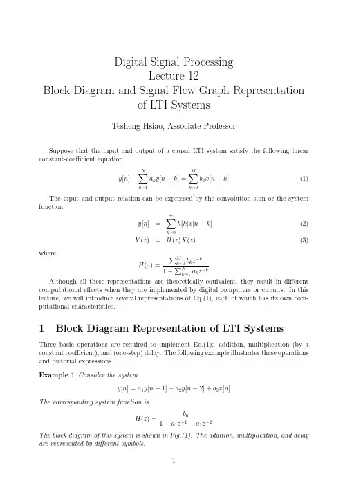
Digital Signal ProcessingLecture12Block Diagram and Signal Flow Graph Representationof LTI SystemsTesheng Hsiao,Associate ProfessorSuppose that the input and output of a causal LTI system satisfy the following linear constant-coefficient equationy[n]−N∑k=1a k y[n−k]=M∑k=0b k x[n−k](1)The input and output relation can be expressed by the convolution sum or the system functiony[n]=∞∑k=0h[k]x[n−k](2)Y(z)=H(z)X(z)(3)whereH(z)=∑Mk=0b k z−k 1−∑Nk=1a k z−kAlthough all these representations are theoretically equivalent,they result in different computational effects when they are implemented by digital computers or circuits.In this lecture,we will introduce several representations of Eq.(1),each of which has its own com-putational characteristics.1Block Diagram Representation of LTI SystemsThree basic operations are required to implement Eq.(1):addition,multiplication(by a constant coefficient),and(one-step)delay.The following example illustrates these operations and pictorial expressions.Example1Consider the systemy[n]=a1y[n−1]+a2y[n−2]+b0x[n]The corresponding system function isH(z)=b01−a1z−a2zThe block diagram of this system is shown in Fig.(1).The addition,multiplication,and delay are represented by different symbols.Figure 1:Block diagram of the system in Example 1Consider the general case,i.e.the system described by Eq.(1).The block diagram is shown in Fig.(2).This realization is called direct form I .In direct form I realization,the output is obtained through two steps:v [n ]=M ∑k =0b k x [n −k ]y [n ]=N ∑k =1a k y [n −k ]+v [n ]or equivalently,V (z )=H ma (z )X (z )={M ∑k =0b k z −k }X (z )Y (z )=H ar (z )V (z )={11−∑N k =1a k z −k }V (z )and H (z )=H ar (z )H ma (z ).Figure 2:Direct Form I representation of an LTI systemSince both H ar(z)and H ma(z)are LIT systems.We can exchange the order and leave the results unaltered.Hence the system can be implemented in a different way:W(z)=H ar(z)X(z)Y(z)=H ma(z)W(z)or equivalently,w[n]=N∑k=1a k w[n−k]+x[n]y[n]=M∑k=0b k w[n−k]This results in the block diagram in Fig.(3).Figure3:Direct Form II representation of an LTI system In Fig.(3),the two columns of delays contains the same values(w[n−k]);hence they can be combined into one column of delays as shown in Fig.(4).The realization in Fig.(4) is called direct form II or canonic direct form.One distinct property of direct form I and II is the number of delays.In other words, the required size of storage space(memory or register)is different.Direct form I contains N+M delays whereas direct form II has max{M,N}delays.Hence direct form II is more efficient in terms of space usage.An implementation with the minimum number of delay elements is commonly referred to as a canonic form implementation.Example2Consider the LTI systemH(z)=1+2z−11−1.5z−1+0.9z−2The direct form I and II implementation are shown in Fig.(5)and Fig.(6)respectively.Figure4:Direct Form II representation of an LTI systemFigure5:Direct form I of Example22Signal Flow Graph Representation of LTI Systems Instead of using block diagrams introduced in the previous section,we usually use signal flow graph to represent a system described by Eq.(1)because signalflow graphs are more compact.A signalflow graph consists of nodes and directed branches.A node denotes a variable or a sequence.A node could have several entering and leaving branches.A branch connects a pair of nodes with an arrow denoting the direction.Each branch represents a linear operation,such as multiplication or delay,on the departure node.The operation carried out by each branch is denoted by that branch.It denotes the unity gain multiplication if there is no notation associated with the branch.The value of a node is the sum of all entering branches.There are two special nodes in the signalflow graph.Source nodes are nodes that have no entering branches.Source nodes are used to represent the injection of external inputs or signal sources into the graph.Sink nodes are nodes that have only entering branches.Sink nodes are used to extract outputs from the graph.Figure6:Direct form II of Example2Fig.(7)illustrates the direct form II and signalflow graph of afirst order IIR system. The equations represented by Fig.(7b)arew1[n]=aw4[n]+x[n]w2[n]=w1[n]w3[n]=b0w2[n]+b1w4[n]w4[n]=w2[n−1]y[n]=w3[n]These equations can be rearranged,eliminating redundant variables,and becomew2[n]=aw2[n−1]+x[n]y[n]=b0w2[n]+b1w2[n−1]which are exactly the equations represented by direct form II.Figure7:(a)Direct form II(b)Signal Flow GraphOn the other hand,given a signalflow graph,we want to derive the system function from it.The z-transform techniques would be useful in this case,as explained by the following example.Example3Given the signalflow graph in Fig.(8).We can write down the equations for each node:w1[n]=w4[n]−x[n]w2[n]=αw1[n]w3[n]=w2[n]+x[n]w4[n]=w3[n−1]y[n]=w2[n]+w4[n]Take z-transform on both sides,we haveW1(z)=W4(z)−X(z)W2(z)=αW1(z)W3(z)=W2(z)+X(z)W4(z)=z−1W3(z)Y(z)=W2(z)+W4(z)Eliminate W1(z)and W3(z),we obtainW2(z)=α(W4(z)−X(z))(4)W4(z)=z−1(W2(z)+X(z))(5)Y(z)=W2(z)+W4(z)Solving Eq.(4)and Eq.(5)simultaneously,we haveW2(z)=α(z−1−1)1−αz−1X(z)W4(z)=z−1(1−α)1−αz−1X(z)Therefore the system function isY(z)=(α(z−1−1)+z−1(1−α)1−αz−1)X(z)=(z−1−α1−αz−1)X(z)Note that the direct form I representation of the system function is shown in Fig.(9).In direct form I representation,2delay elements and two multiplications are required.Direct form II representation needs one delay element but still two multiplications.In the represen-tation of Fig.(8),only one delay element and one multiplication is required.Figure8:Signalflow graph for Example3Figure9:Direct Form I representation of the system function in Example3。


mit单变量微积分讲义lecture12 解释说明1. 引言1.1 概述在本篇长文中,我们将详细讨论MIT单变量微积分讲义的第12讲。
在这节课中,我们将重点介绍和解释一些重要的概念和原理,以帮助读者更好地理解微积分的基础知识。
1.2 文章结构本文分为六个主要部分以及一个大纲部分。
在大纲部分,我们提供了整篇文章的框架结构,使读者能够清晰地了解各个小节之间的逻辑关系。
接下来,正文部分将开始详细介绍与解释第12讲中所涉及到的主题和概念。
1.3 目的本文的目的是通过对MIT单变量微积分讲义lecture12进行全面而详细的解读,帮助读者加深对微积分知识的理解和掌握。
通过对每个章节进行详细阐述,并总结各章节的要点,我们旨在使读者能够更好地应用微积分原理解决实际问题,并为进一步学习和探索微积分打下坚实基础。
以上是关于文章“1. 引言”部分内容的详细说明。
2. 正文正文部分是对MIT单变量微积分讲义lecture12的详细解释和说明。
本篇文章将从以下几个方面展开讨论。
首先,我们将对讲义中提到的概念和理论进行介绍和解释。
这包括但不限于微积分的基本概念、函数的极限、导数和微分等重要内容。
我们将从直观的角度出发,通过具体的例子来说明这些概念和理论在实际问题中的应用。
其次,我们将深入探讨讲义中涉及到的各种技巧和方法。
这些技巧包括但不限于求导法则、曲线的切线与法线、泰勒级数展开等等。
我们会结合实例详细说明这些技巧的运用步骤,并举例说明在实际问题中如何应用这些方法来解决数学难题。
此外,我们还会详细介绍讲义中所涉及到的一些重要定理和公式。
例如,拉格朗日中值定理、洛必达法则以及牛顿-莱布尼茨公式等。
我们将对这些定理和公式进行证明,并解释其背后的数学原理及其在微积分领域中的应用。
最后,我们将对讲义中的例题进行逐一分析和解答。
通过具体实例的讨论,读者将更好地理解和掌握讲义中所介绍的知识点,并能够灵活应用到其他类似问题中去。
在本节内容的整理中,将尽力保持逻辑清晰、条理性强,并且注重与读者之间的沟通。
CS500:Fundamentals of Algorithm Design and Analysis Spring2012
Lecture12—Feb13,2012
Prof.Will Evans Scribe:Shuang Yu In this lecture we:
•Discussed string matching using Finite State Machine;
•Discussed string matching using Knuth-Morris-Pratt Finite State Machine.
1String Matching using Finite State Machine
1.1Problem Statement:
Input:
Pattern P=p1p2...p m
Text T=t1t2...t n
From alphabet=Q,t i∈Q for all i,p j∈Q for all j,n>>m.
Find:
index offirst occurrence of P in T.
1.2Finite State Machine(FSM):
Design a machine that scans text from left to right,and stops if it sees the pattern.
Example:
P=ABAC,Q={A,B,C,D}
Rules:
Create transition:
for each proper prefix R of pattern P
and each charactre x∈Q
where S is the longest prefix of P that is also a suffix of Rx
Running time:
•O(n)once FSM is built[machine takes constant time to consume one text character and
make its transition]
•time to construct FSM≥|Q|·m[because there are this many transitions](there is a
way to construct FSM in O(|Q|·m)time)
•Total time:O(n+|Q|·m)
2Knuth-Morris-Pratt Finite State Machine(KMP-FSM)
Idea:Have a simple”failure”arrow for each state
Example for P=ABAC:
If fail to match the next character in text then follow failure arrow but do not move pointer in text(rescan next text character)unless fail inφ-state.
Text T=A B D A A B A D A B A C
State0120112301234
001
where state0isφ-state,state1is state A,state2is state AB,etc.
Running time:
•#of forward arrows(success)traversed+#of back arrows(failure)traversed≤2n
•Because we know:#of forward arrows traversed≤n(each consumes text character)
#of forward arrows traversed≥#of back arrows traversed
Build KMP-FSM:
1.Make”backbone”(all forward edges)
pute back edges
S is the longest prefix of P that is also a proper(i.e.not R itself)suffix of R
Define:
back[i]is the longest j such that p1p2...p j is a proper suffix of p1p2...p i
back[i]is destination of back edge from state i
state0is initial state
Back calculation:
back[1]=0
j=0
for i=2to m do
while j>0and p j+1=p i do
j=back[j]
if p j+1=p i then j=j+1
back[i]=j
Idea:
Add back edges to states in left to right order,use what has been constructed to
find next back edge quickly.。