carbon offset potentials of four alternative-Mitigation and a Adaptation

备战2022年中考英语考前时事热点话题阅读+题型专练热点热点102 认识减少碳排放的作用一、阅读理解1Climate change is a global challenge. One way to fight it is by reducing the amount of carbon dioxide in the air. New research shows that trees planted in China have helped in this fight.A recent study in the journal Nature shows that the amount of carbon dioxide absorbed (吸收) by new forests in two parts of China is more than we thought. These areas are in the northeastern Heilongjiang and Jilin provinces and the southwestern Yunnan and Guizhou provinces and Guangxi Zhuang autonomous region. They make up about 35 percent of China’s landbased (基于陆地的) carbon sinks (碳汇). A carbon sink is a natural area like a forest or ocean that absorbs morecarbon dioxide than it emits (排放). Carbon sinks help to reduce the amount of CO2 in the atmosphere.China’s goal is to peak (达到峰值) its CO2 emissions (排放) before 2030 and reach carbon neutrality (中和) by 2060, Xinhua reported. Carbon neutrality refers to removing as much CO2 as one puts into the air.According to stud y coauthor Yi Liu at the Chinese Academy of Sciences, “the afforestation (植树造林) activities described in our Nature paper will play a role in reaching that goal.”1. A recent study in Nature shows that ________.A. China has serious air pollutionB. China has planted the most trees in the worldC. China has fewer CO2 emissions (排放) nowD. China has planted fewer trees2. Carbon sinks will ________.A. absorb more CO2 than they emitB. give off CO2 emissions more quicklyC. release less CO2 into the airD. have no CO2 in their air3. According to Xinhua, China ________.A. is the world’s largest emitter of CO2B. will bring CO2 emissions down after 2030C. will not release CO2 in the futureD. will reach carbon neutrality by 20304. Which of the following is NOT TRUE in the passage?A. One way to fight climate is by reducing the amount of carbon dioxide in the air.B. Trees planted in China have helped fight against climate change.C. New forests in two parts of China absorbed more carbon dioxide than we thought.D. 35 percent of China’s land has been affected by CO2 emission.5. What do we know from the story?A. It takes a long time for carbon sinks to form.B. Climate change is no longer a serious problem.C. More trees will be planted in China in the future.D. China has beaten climate change.2Did you see snow in your home town last winter? Did you feel it was warmer than before? “There have been 21 warm winters in China since 1986,” said scientists. They also said that in the past 100 years, as the g lobal (全球的) temperatures went up by 0.74 ºC, the temperature in North China has gone up by 1.4 ºC in only 50 years.China needs to take quick action to cut carbon dioxide emission (排放), because it’s the main reason for global warming. We plan to cut energy use by 20% and pollution emission by 10% in the 11th FiveYear Plan.Can you slow global warming? Sure! You and your family can take steps to cut the amount of carbon dioxide that is sent out into the air.Here are some pieces of advice to help you save the earth. Wear used clothes. Wearing your brother’s, sister’s or dad’s old Tshirts means you save the energy.Ride on the bus. Taking a bus saves a lot of oil every year.Open the window. Don’t use the air conditioner (空调), and let some fresh air in. When you have to use it, set the temperature higher in summer and lower in winter to save energy.Make small changes in your daily life. Don’t use paper cups, bags and boxes.It’s time for all of us to do something to save the earth.6. Since more than 30 years ago, there has been _______ according to the passage.A. more and more snowB. more cold wintersC. the rising of the temperature in South ChinaD. higher and higher global temperature7. The main reason for global warming is _______.A. the oilB. carbon dioxide emissionC. paper cups, bags and boxesD. televisions and puters8. The word “energy” in the second paragraph means “_______”.A. 活力B. 干劲C. 精力D. 能源9. Which of the following is true?A. Using air conditioners may be a waste of energy.B. It’s funny to wear your dad’s old Tshirts.C. Taking a bus wastes a lot of oil every year.D. Using paper bags saves energy a lot.10. The passage is mainly about the ways to _______.A. slow down global warmingB. make energyC. change our daily lifeD. change the world weather3A large part of China experienced larger amounts of smog (雾霾) than usual this January and the air was badly polluted. The distance one could see was shorter than 1,000 meters in Beijing, Tianjin, and the provinces of Hebei, Henan, Shandong and Anhui. In some areas, it was down to 200 meters.People usually set off firecrackers (爆竹) to celebrate Spring Festival. But because of the smog, this year seemed very quiet. It was really different. A man called Zhang Wei said that his fri ends and he hadn’t set off a single firecracker.“ We all suffered from last month’s smog. If we don’t call an end to the firecrackers, the environment will get worse and worse during the holiday. ” said Zhang Wei. He called on more people to set off fewe r firecrackers during this year’s Spring Festival by putting up a notice in his neighborhood.More Chinese looked forward to celebrating the holiday in a greener way. They decided not to set off firecrackers. They also decided not to waste food. They said the new celebrations sounded fashionable.To clean the sky, more than ten provinces including Guangdong, Zhejiang and Jiangsu have started to use national 4 standard (标准), which is expected to reduce vehicle emission (车辆排放) by 30% to 50%. Beijing even has started to use the stricter national standard.We still have a lot to do to improve the air quality. For example, using public transportation as much as possible is not a hard thing for us to do, but it matters a lot.11. What happened in a large part of China this January?A. There was a serious smog.B. People set off lots of firecrackers.C. There was a heavy rain.D. Many car accidents happened.12. Where is the most strict standard for vehicle emission used?A. In the countryside.B. In a few areas.C. In the small cities.D. In the big cities.13. Which of the following is Not true according to the passage?A. Zhang Wei didn’t set off a single firecracker this Spring Festival.B. We should use more public transportation to help reduce the air pollution.C. Zhejiang has started to use national 4 standard to reduce vehicle emission.D. More Chinese think the celebration of setting off firecrackers is fashionable.14. What’s the best title for the passage?A. How to reduce the vehicle emissionB. How to improve the air qualityC. What do Chinese do in Spring FestivalD. Using public transportation4A large part of China experienced larger amounts of smog (雾霾) than usual and the air was badly polluted.The distance one could see was shorter than 1,000 meters in Beijing, Tianjin, and the provinces of Hebei, Henan, Shandong and Anhui.In some areas, it was down to 200 meters.People usually set off firecrackers (爆竹) to celebrate the Spring Festival.But because of the smog, this year seemed very quiet.It was really different.A man called Zhang Wei said that his friends and he hadn't set off a single firecracker.“We all suffered from last month's smog.If we don't call an end to the firecrackers, the environment will get worse and worse during the holiday.” Said Zhang Wei.He called on more people to set off fewer firecrackers during this year's Spring Festival holiday by putting up a notice in his neighborhood.More Chinese looked forward to celebrating the holiday in a greener way.They decided not to set off firecrackers.They also decided not to waste food.They said that the new celebrations sounded fashionable.To clean the sky, more than ten provinces including Guangdong, Zhejiang and Jiangsu have started to use national 4 standard (标准), which is expected to reduce (减少) vehicle emission (车辆排放) by 30% to 50%.Beijing even has started to use the stricter national 5 standard.We still have a lot to do to improve the air quality.For example, using public transportation as much as possible is not a hard thing for us to do, but it matters a lot.15. What happened in a large part of China this January?A. It experienced larger amounts of smog.B. People set off lots of firecrackers.C. There was a heavy rain.D. Many car accidents happened.16. How do people usually celebrate the Spring Festival in China?A. By putting up a noticeB. By setting off firecrackers.C. By not wasting food.D. By using public transportation.17. How many provinces have started to use national 4 standard?A. Three.B. Six.C. Eight.D. More than ten.18. Which of the following is NOT true according to the passage?A. Zhang Wei didn't set off a single firecracker this Spring Festival.B. We should use more public transportation to help reduce the air pollution.C. Zhejiang has started to use national 4 standard to reduce vehicle emission.D. More Chinese think the celebration of setting off firecracker is fashionable.19. What's the best title for the passage?A. How to Reduce the Vehicle EmissionB. How to Improve the Air QualityC. What Do Chinese Do in the Spring FestivalD. Using Public Transportation5Recently, the term “carbon neutral (碳中和)” has been used frequently at some important meetings in many countries. Many countries have put forward the goal of striving (奋斗目标) to be carbon neutral. China is expected to be carbon neutral by 2060. So, as middle school students, what can we do to protect the environment and live a low carbon life? Here are some suggestions for you.Travel in a green way. Now more Chinese people have cars of their own. It has brought us a lot of benefits but has created some serious problems as well. So we’d better do more walking, cycling and less driving. By doing so, we can save energy and reduce pollution.Cut down white pollution. We should reduce the pollution of plastic bags. When you go to the supermarket, bring your own shopping bags.Save water. Lack (缺乏) of water resources will affect the ecological environment (生态环境). So please turn off the tap after using it.Sort (分类) the rubbish. Doing garbage classification (垃圾分类) in a right way can turn waste into wealth.Plant more trees. Planting more trees means cutting down and reducing the carbon footprint (碳足迹) and spreading of greenhouse gases (气体).Use both sides of the paper. The paper production process uses a lot of trees.Now is the time that we should take up our responsibility to protect our environment from being polluted.Let’s join our hands and take actions immediately.20. How many suggestions does the writer give in the passage to be carbon neutral?A. 5B. 6C. 7D. 821. In order to protect the environment and live a low carbon life, we can _________ .①walk, cycle more and drive less②use plastic bags while shopping③use only one side of the paper④tum off the water after using it⑤do garbage classification in a right wayA. ①②③④⑤B. ①③④⑤C. ①②⑤D. ①④⑤22. The purpose of the passage is _________ .A. to call us to cut down white pollutionB. to advise us to travel in a green wayC. to give suggestions on why to plant more treesD. to give advice on how to protect the environment23. What is the main idea of the passage?A. Live a low carbon life.B. Sort the rubbish.C. Travel in a green way.D. Save the world.6Now too much CO2 makes the Earth warmer and warmer, and brings bad effect to people. To save our Earth, a new lifestyle called lowcarbon life bees popular. Low carbon means low energy and no waste. It is necessary for everybody to learn to live a lowcarbon life.To live a lowcarbon life, we’d better save as much energy as we can. For example, turn off the lights and TV when you don’t use them, use cold water to wash clothes or dishes; take a short shower and try to take a cold one when the weather gets warm; don’t do the c ooking with electricity.To live a lowcarbon life, we should eat less meat. Being a vegetarian can help reduce(减少) one and a half tonof carbon dioxide a year, but keeping animals for food produces even more carbon dioxide than all the cars do in the world.To live a lowcarbon life, we should plant more trees. Trees are very important for us. They can not only produce oxygen for us to breathe and keep the air clean, but also take in the harmful gases from the air. To protect trees we should stop people from cuting down trees and plant as many trees as we can.If we can keep them a habit in our daily life, the earth will bee a safer planet for us to live on.24. Why does lowcarbon life bee popular?A. Because it can protect animals.B. Because it can save the earth.C. Because it can protect trees.D. Because it can clean water.25. How many kinds of way of living a lowcarbon life are talked about in the passage?A. Three.B. Four.C. Five.D. Six.26. What can we do to make carbon dioxide bee less?A. We can use cold water in our life.B. We can try to use less water.C. We can eat too much meat.D. We can take a bath.27. What does the underlined word “them” refer to?A. The ways to protect trees.B. The ways to keep animals for food.C. The ways to live a fortable life.D. The ways to live a lowcarbon life.二、阅读还原（7选5）In 2019, Europe faced a recordbreaking heat in summer. It was so hot there that you could have even fried an egg on the pavement. Such extreme temperatures are also killing people. ___28___ For example, the melting glaciers(冰川融化). As a result of it, coastal cities from America to Asia are drowning. You may also know another result of global warming: the thawing permafrost(冻土融化). Permafrost usually exists in polar regions. It’s underground so il that’s always frozen. The thawing permafrost further warms up the earth.___29___ Scientists believe that greenhouse gas emission(温室气体排放) is an important cause leading to the sudden increase in temperatures globally. The greenhouse gases are known for keeping heat. And these gas emissions mostly e from plants, automobiles and factories that use fossil fuels like coal and petrol etc. ___30___ ___31___ There are a lot of ways. For example, using public transport, planting trees and recycling your waste like plastics, are all useful ways to reduce your carbon footprint. Turning off electronic equipments when you are not using them can also be amazingly good for this.___32___ Turning it down 2 degrees in winter and up 2 degrees in summer could save nearly a kilogram of carbon dioxide every year.Everyone should play their part in to slow down global warming because we are not saving the Earth, we are saving ourselves.A. So what can we do to slow down the global warming?B. That’s not the worst.C. The hot weather also leads to other serious results.D. You may want to know what exactly causes global warming.E. That’s to say, we or human activities are responsible for global warming.F. Adjusting your temperature of your air conditioners is also suggested.G. Let’s take actions to stop the global warming.三、阅读填表Scientists said that in the past 100 years, as the global(全球的) temperatures went up by 0.74℃, the temperature in North China has climbed 1.4℃ in only 50 years.China needs to cut down carbon dioxide(二氧化碳) emission(排放)，because it can make the global warm. The good news is that China has seen the importance of going green. China has decided to cut energy use down by 20% and pollution emission by 10% in the 11th FiveYear Plan.Can you slow down global warming? Sure! You and your family can take some steps.Here are some pieces of advice to help you save the earth.Wear used clothes. It means that you save the energy when you wear your brother’s, sister’s or dad’s old Tshirts.Change your light bulbs(灯泡). Us e energysaving light bulbs. And don’t forget to turn off the lights when you leave a room and turn off your television and puter when you don’t need them.Take a bus. Taking a bus saves a lot of oil(石油) every year.Say no to plastic bags. The next time your parents go to the market, ask them to use baskets.Open the windows. Don’t use the air conditioner(空调). Let some fresh air in. When you have to use the conditioner, set the temperature higher in summer and lower in winter to save energy.四、完形填空Did you feel it was warmer than before?“There have been twentyone ____38____winters in China since 1986,” said scientists. “____39____the past 100 years, as the world temperature has been up by 0.74 °C , the temperature in North China has ____40____1.4 °C in only 50 years.”China needs to take quick actions to____41____ carbon dioxide (二氧化碳) emission (排放) because it’s the main reason for world warming. The good news is that China has seen the importance of going_____42_____ China sets the goal of cutting energy use by 20% and pollution emission by 10% in the 11th FiveYear Plan.Here is some advice for you.____43____used clothe s such as your brother’s, sister’s or dad’s old Tshirts means you ___44___ energy; And don’t forget to_____45_____the lights when you leave a room and turn off your television and puter when they are not____46____! Besides, taking a bus saves a lot of oil every year. Also open a window and try not to use the air conditioner (空调). If necessary, set the temperature_____47_____ in summer and lower in winter to save energy; It isn’t good to use paper cups, bags or boxes in our daily life.38. A. cool B. hot C. cold D. warm39. A. during B. for C. since D. after40. A. climbed B. went C. arrived D. got41. A. increase B. improve C. cut D. break42. A. yellow B. green C. black D. blue43. A. Wearing B. Dressing C. Buying D. Selling44. A. use B. find C. save D. keep45. A. turn on B. turn off C. turn up D. turn over46. A. in use B. on business C. at present D. for fun47. A. lower B. higher C. taller D. brighter五、短文汉语提示填空Save Our EnvironmentThere is no doubt that global warming has bee one of the b___48___ problems we face today. So it's i___49___ for us to protect our environment.As middle school students, what can we do? First of all, t___50___ to take bicycles and public transportation to school instead of cars b___51___ it will make less CO2. It can not only be good for our health, but also make it possible for us to get closer t___52___ nature. Then, it's necessary to p___53___ up rubbish and put it into dustbin(垃圾桶). Planting more trees can also help a lot. And we should never f___54___ to turn off the lights when we leave the classroom. What's more, why not r___55___ water and paper to live a lowcarbon life?I think it's everyone's duty to help our Earth. And even the simplest activities can make a real d___56___ to our environment. So don't put it off! Let's do what we can to p____57____ our home. I believe we will make our world more and more beautiful.。

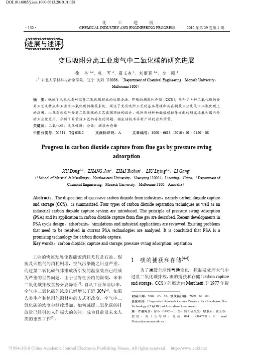
CHEMICAL INDUSTRY AND ENGINEERING PROGRESS 2010年第29卷第1期·150·化工进展变压吸附分离工业废气中二氧化碳的研究进展徐冬1,2，张军2，翟玉春1，刘丽影1,2，李刚2（1东北大学材料与冶金学院，辽宁沈阳 110086；2 Department of Chemical Engineering，Monash University，Melbourne 3800）摘要：概述了未来人类对过量二氧化碳排放的处理办法，即碳的捕获和存储（CCS）。

简介了4种二氧化碳的分离工艺及特点和工业中二氧化碳的捕获系统。

阐述了变压吸附工艺的基本原理和其在捕获工业废气中二氧化碳上的应用，以及变压吸附分离二氧化碳的工艺在循环结构设计、吸附剂材料和数值模拟等方面的研究进展和国内外的工业化应用。

分析了目前该工艺仍存在的问题，指出该技术具有广阔的应用前景。

关键词：二氧化碳；变压吸附；分离；捕获和存储中图分类号：X 511；TQ 028.2 文献标识码：A 文章编号：1000–6613（2010）01–0150–08 Progress in carbon dioxide capture from flue gas by pressure swingadsorptionXU Dong1,2，ZHANG Jun2，ZHAI Yuchun1，LIU Liying1,2，LI Gang2（1 School of Material & Metallurgy，Northeastern University，Shenyang 110004，Liaoning，China；2 Department of Chemical Engineering，Monash University，Melbourne 3800，Australia）Abstracts：The disposition of excessive carbon dioxide from industries，namely carbon dioxide capture and storage (CCS)，is summarized. Four types of carbon dioxide separation techniques as well as an industrial carbon dioxide capture system are introduced. The principle of pressure swing adsorption (PSA) and its application in carbon dioxide capture from flue gas are described. Recent developments in PSA cycle design，adsorbents，simulations and industrial applications are reviewed. Existing problems that need to be resolved in current PSA technologies are analysed. It is concluded that PSA is a promising technology for carbon dioxide capture.Key words：carbon dioxide; capture and storage; pressure swing adsorption; separation工业的快速发展使得能源消耗尤其是石油、煤炭及天然气的消耗剧增，空气污染随之日益严重。

自考英语二模拟试题及答案I. Multiple Choice Questions (多项选择题)1. Which of the following is NOT a reason why people might choose to study abroad?A. To improve language skills.B. To experience a different culture.C. To gain a higher salary.D. To make new friends.Answer: C2. The main idea of the passage is that:A. Learning a new language is difficult.B. Technology has made communication easier.C. Environmental issues are a global concern.D. Education is becoming more accessible.Answer: D3. According to the speaker, what is the most important factor in being successful in business?A. Having a good education.B. Being able to work hard.C. Networking with the right people.D. Having a lot of capital.Answer: CII. Reading Comprehension (阅读理解)Passage 1The rise of the internet has revolutionized the way we communicate. It has made it possible for people to connect with each other from all over the world in a matter of seconds. This has led to a surge in online communities where people can share ideas, collaborate on projects, and form friendships. However, the anonymity of the internet can also lead to negative behaviors, such as cyberbullying and the spread of misinformation.Questions:4. What is the main advantage of the internet mentioned in the passage?A. Speed of communication.B. Cost-effectiveness.C. Accessibility of information.D. Entertainment value.Answer: A5. What is identified as a potential negative aspect of the internet?A. Privacy concerns.B. Cyberbullying.C. Technical difficulties.D. Limited access for some users.Answer: BPassage 2Climate change is one of the most pressing issues facing the world today. It is caused by the increase in greenhouse gases in the atmosphere, primarily due to human activities such as burning fossil fuels and deforestation. The effects of climate change are already being felt around the globe, with more frequent and severe weather events, rising sea levels, and loss of biodiversity. It is crucial for governments, businesses, and individuals to take action to reduce carbon emissions and mitigate the impacts of climate change.Questions:6. What is the primary cause of climate change?A. Natural disasters.B. Greenhouse gases.C. Volcanic eruptions.D. Cosmic events.Answer: B7. What is one of the effects of climate change mentioned in the passage?A. Increased agricultural yields.B. More stable weather patterns.C. Rising sea levels.D. A decrease in biodiversity.Answer: CIII. Vocabulary and Structure (词汇与结构)8. The company's profits have ________ by 20% this quarter compared to the same period last year.A. increasedB. decreasedC. remainedD. fluctuatedAnswer: A9. Despite the heavy rain, the construction work was ________ on schedule.A. delayedB. advancedC. maintainedD. suspendedAnswer: CIV. Cloze Test (完形填空)[Passage略]10. The correct answer to fill in the blank in the first sentence is:A. rarelyB. seldomC. oftenD. frequentlyAnswer: C11. The word that best fits the blank in the third sentence is:A. solutionB. problemC. challengeD. opportunityAnswer: AV. Writing (写作)12. Write an essay of about 200 words on the topic: "The Impact of Social Media on Modern Society."[Essay略]Answer: (学生需自行撰写一篇200字左右的短文)自考英语二模拟试题参考答案I. Multiple Choice Questions (多项选择题)1. C2. D3. CII. Reading Comprehension (阅读理解)4. A5. B6. B7. CIII. Vocabulary and Structure (词汇与结构)8. A9. CIV. Cloze Test (完形填空)10. C11. AV. Writing (写作)12. [Essay略] (学生需自行完成写作部分)。

碳达峰核心指标测算英文回答：Key Indicators for Carbon Peaking Measurement.Determining the primary indicators for carbon peaking involves assessing both quantitative and qualitative factors. Quantitatively, this includes:1. Cumulative Carbon Emissions (CCE): The total amount of carbon dioxide (CO2) emitted over a specified period. CCE provides insight into the historical and ongoing contributions to climate change.2. Carbon Intensity (CI): The ratio of carbon emissions to economic activity, expressed in units of CO2 per unit of GDP. Lower CI indicates a shift towards cleaner energy sources.3. Carbon Removal (CR): The process of capturing andstoring carbon dioxide from the atmosphere or other sources. CR helps offset carbon emissions and mitigate climate change impacts.Qualitatively, carbon peaking measurement considers:4. Policy Framework: The effectiveness of government policies and regulations in promoting carbon reduction.This includes carbon pricing, emissions trading, and renewable energy incentives.5. Technological Advancement: Progress in developinglow-carbon technologies and carbon capture and storage methods. Technological innovation accelerates thetransition to a low-carbon economy.6. Behavioral Changes: Shifts in consumer and industry behaviors towards reduced carbon consumption. Public awareness and education play a crucial role in promoting sustainable practices.中文回答：碳达峰核心指标测算。

碳排放外文翻译--全球碳披露激励设置：实证研究中文3265字,1825单词，1.1万英文字符本科毕业论文外文资料翻译系别：经济系专业：会计学姓名：学号：2014 年 4 月 30 日外文原文CarbonDisclosure Incentives ina Global Setting:An Empirical InvestigationI. IntroductionWe investigate the country level factors that influence a firm?s decision to participate in and disclose corporate carbon emission information. Concern over climate change and its potential impact on corporate activities is garnering increased attention among company stakeholders and regulators. In response, the field of accounting is increasingly being shouldered with the responsibility of understanding the role of reporting corporate environmental performance, as well as financial performance (Hopwood, 2009). In particular companies are being confronted with the challenges of accounting for and reporting of greenhouse gas or carbon emissions.While carbon disclosure is predominately voluntary, mandatory legislation is increasingly being proposed or implemented throughout the world. For example, the U.S. Environmental Protection Agency (EPA) has proposed a mandatory greenhouse gas reporting rule to collect accurate and comprehensive corporate emissions data in order to informfuture policy decisions. Likewise, public demands for corporations and financial markets to address climate change reporting prompted the formation of the Climate Disclosure Standards Board (CDSB) at the 2007 Annual World Economic Forum. The goal of the CDSB is to advance climate changedisclosure in mainstream corporate reporting by developing a global framework and standards for carbon emission disclosures (CDSB 2007).II. Carbon Disclosure and Related Disclosure LiteratureCarbon Disclosure ProjectThe CDP has become a standard for carbon emission reduction, providing an avenue and repository for the largest corporations in the world. It is an independent not-for-profit organization, established December 4, 2002, to facilitate communication between shareholders and corporations in an effort to develop a comprehensive response to global climate change. Because firm specific responses to each questionnaire, including a decline or non-response action, are displayed on the CDP?s website, motivation increases for firms to participate in the questionnaire process and disclose results. Each year the CDP lists all firms requested to participate and discloses specific responses to a comprehensive questionnaire regarding corporate carbon emissions and climate change.Extant voluntary disclosure literature is limited with regards to studies concerning carbon reporting information. Growing more important for stakeholders, regulators, and practitioners is the need to better understand the motivation for these disclosures as firm risk of potential legal liabilities related to corporate influence on climate change increases. If they do not adequately disclose their climate change risks, shareholders cansue the company and pursue separate actions against directors and managers who might not have satisfied their fiduciary responsibility in relation to informing investors (Johnson 2007). The first of such lawsuits came in 2004, when the attorney generals from eight states and New York City filed a climate change …nuisance? lawsuit against the top five U.S. emitters of carbon dioxide (Baue 2004). In response to these fears, firms are increasing their environmental strategies and related disclosures.Environmental Disclosure LiteratureMany environmental accounting studies have attempted to determine the incentives which motivate firms to disclose environmental information. These studies are often limited to settings which involve firms within only one country or in a small set of countries. Barth et al. (1997) investigate those U.S. firms included in environmental liability intensive industries which are named as Environmental Protection Agency (EPA) potentially responsible parties (PRP) and determine that increased environmental disclosure is associated with regulatory influence, allocation uncertainty, litigation and negotiation concerns, capital market concerns, and other regulatory effects.V oluntary Disclosure LiteratureThe second stream of research supporting our study focuses more generally on voluntary disclosure incentives in an international, cross-country setting. A recent study by Cahan et al. (2005) examines how firm level variation in voluntary disclosure is affected by global diversification. Studies by Bushman et al. (2004) and La Porta et al. (1998) investigate variation in cross-country determinants of voluntary disclosure at the country level.Additionally, Jaggi and Low (2000), Hope (2003), and Francis et al. (2005) examine the influence of country leveland firm level incentives on the level of voluntary disclosure. None of these studies focus on the unique domain of environmental reporting.III. SampleAnd Empirical TestsSampleThe sample firms and disclosure data are gathered from years 1-5 of the CDP. Information pertaining to the environmental regulatory stringency of each country is determined by Esty and Porter (2005). Nationallevel corporate environmental responsiveness is from the 2002 Environmental Sustainability Index (World Economic Forum 2002). The variable for the legal system comes from La Porta et al. (1998) and the data for financial structure comes from Levine (2002). Both the size and leverage of the firm are obtained from Global Vantage. Firm-specific cross-listing is determined by the world?s top six stock exchanges as determined by domestic market capitalization.The initial sample of CDP disclosure firms represented 63 different countries. This initial sample was restricted by country-level data regarding environmental regulatory stringency in Esty and Porter (2005). Data for financial structure (Levine 2002) and legal structure (La Porta et al. 1998) further restricted the country-level data, decreasing the country level coverage to 28 distinct countries. Additional losses from the absence of Compustat data reduced the sample to a final 4799 firm-specific responses, consisting of 2140 unique firms. Appendix provides a detailed list of disclosures by country and by year,provides a summarized list of disclosure level by country. For those firms that chose to disclose, the level of CDP participation is broken down into full participation and those firms only providing areduced level of information. Non-disclosure also includes those firms choosing not to participate.Dependent Variable – Carbon Accounting DisclosureThe existence of carbon disclosure is determined by the 2002 –2006 CDPquestionnaire response results. Since its inception in 2002, the CDP has requested corporate voluntary participation in a carbon disclosure questionnaire aimed at increasing the global climate change communication among corporations, non-governmental organizations, regulators, academics, and all other interested stakeholders. Once sent a questionnaire, the firms decide whether to participate in the process in one of four actions. They can: (1) participate in the questionnaire by providing all requested information, (2) participate in the questionnaire by providing some information, but not all as requested by the CDP, (3) disclose their response or choose to have it noted otherwise as a non-disclosure, (4) choose not to participate at all by communicating such a response or by not responding.Because the methodology for carbon disclosure is so ambiguous and there is a fear of non-comparability, the uncertainty of response to this complex information, and the proprietary cost associated with the knowledge of such information by competitors and environmental advocacy groups alike, it is of interest to empirically determine which country-level characteristics are associated with this global disclosure amongst firms. The CDP setting provides a unique opportunity to test environmental disclosure across country boundaries where the request for information is ubiquitous and comparable. These advantages allow me to conduct multiple analyses. We examinethe determinants of overall disclosure which is denoted by DISC. We then disentangle the firm disclosure decision further to evaluate those firms that choose to fully participate and disclose all requested information, FULLDISC, and those firms that choose only to provide some information and disclose, PIDISC, across countries. We further examine the sample to determine what incentives drive a firm?s decision for initial disclosure (FIRSTDISC), and finally, we examine the incentives driving mere participation in the CDP questionnaire process to deduce the motivatio n to participate in such a resource intensive process, regardless of a firm?s decision to disclose (PARTIC).Concern about carbon emissions, and hence concern about disclosure of carbon emissionlevels, has been expressed by various stakeholders, including corporate executives, boards of directors, investors, creditors, standard setters, government regulators, and NGOs. Indeed, some informed observers expect that the relationship between carbon emissions and global climate change will drive a redistribution of value from firms that do notcontrol their carbon emissions successfully to firms that do (GS Sustain 2009). Using hand-collected carbon emissions data for 2006-2008 that S&P 500 firms disclosed voluntarilyto the Carbon Disclosure Project, we examine two separate, yet, related questions. The first question addresses firm-level characteristics associated with the choice to disclose carbon emissions. Consistent with economic theory, we predict and find a higher likelihood of carbon emission disclosures by firms with superiorenvironmental performance, conditional on firms taking environmentally proactive actions. However, contrary to our predictions based on socio-political theories, we find no association between inferiorenvironmental performance and thelikelihood of disclosing carbon emissions, conditional on firms taking environmentally damaging actions. Further, we predict and find that firms are more likely to voluntarily disclosetheir carbon emissions as the proportion of industrypeer firm disclosers increases. To address the second question concerning the relationship between carbon emission levels and firm value, we correct for self-selection bias caused by firm- and industry-level characteristics associated with the decision to disclose such emissions. We predict and find a negative association between carbon emission levels and firm value. On average, for every additional thousand metric tons of carbon emissions for our sample of S&P 500 firms, firm value decreases by $202,000. Our sensitivity analyses and robustness test results are similar to our main results.In conclusion, we provide evidence on the factors that affect managers? decisions to publicly disclose their carbon emissions. We alsoshow that investors in equity markets are incorporating the effects of carbon emissions intheir valuation decisions. In response to heightened concerns about climate change, proposals to reduce carbon emissions aim to internalize the costs of emitting GHG by requiring the firm to pay for its emissions –the “Polluter Pays Principle.” Although there are no U.S. regulatory penalties currently in place for carbon emissions, our findings suggest that the market finds the frequently unverified, nonfinancial disclosures of carbon emissions useful and implicitly imputes a price to carbon emissions.Environmental ResponsivenessThe 2002 Environmental Sustainability Index is a collaborative effort between YaleUniversity?s Center for Environmental Law and Policy, ColumbiaUniversity?s Center forInternational Earth Science Information Network, and the World Economic Forum (World Economic Forum 2002). This index provides analysis of 142 countries and ranks those countries based on their overall country sustainability. One area of interest in this examination is that of …Social and Institutional Capacity?, which focuses on society?s capacity to improve its environmental performance. One indicator involved in this measure is environmental responsiveness and includes five specific measures. First, it measures the number of ISO 14001 certified companies per million dollars in GDP, which is a set of environmental management standards to assists firms in minimizing how their operations might negatively affect the natural environment. A second indicator of environmental responsiveness is firm existence on the Dow Jones Sustainability Group Index.Third, the index evaluates the average Innovest EcoValue ratios of firms in each country.This rating methodology assesses each country?s strategies to improve environmental performance, reduce environmentally-related risk, and the capacity for business to develop new opportunities through environmentally-oriented investments. Fourth, they examine the level of corporate concern for environmental sustainability by determining firm membership in the World Business Council for Sustainable Development. Finally, the index evaluates the private sector environmental innovation.(From: Journal ofinternational financial management&accountingV olume 23)外文资料翻译译文全球碳披露激励设置：实证研究一、引言我们调查的国家一级因素影响着公司的决定，参加并披露企业碳排放信息。

关于co2 offseting英语作文English: Carbon offsetting is a way for individuals or organizations to compensate for their carbon footprint by investing in environmental projects that reduce greenhouse gas emissions. This can include projects such as reforestation, renewable energy, or energy efficiency initiatives. By purchasing carbon offsets, individuals or companies can help balance out their own carbon emissions by supporting projects that have a positive impact on the environment. While carbon offsetting is not a perfect solution to climate change, it can be a useful tool in combination with efforts to reduce emissions at the source. Additionally, carbon offsetting can help raise awareness about the importance of taking action to mitigate climate change and encourage a shift towards more sustainable practices.中文翻译: 碳抵消是个人或组织通过投资减少温室气体排放的环境项目来补偿其碳足迹的一种方式。

2023年高考英语外刊时文精读精练(14)Climate change and coral reefs气候变化与珊瑚礁主题语境：人与自然主题语境内容：自然生态【外刊原文】（斜体单词为超纲词汇，认识即可；下划线单词为课标词汇，需熟记。

）Human beings have been altering habitats—sometimes deliberately andsometimes accidentall y—at least since the end of the last Ice Age. Now, though, that change is happening on a grand scale. Global warming is a growing factor. Fortunately, the human wisdom that is destroying nature can also be brought to bear on trying to save it.Some interventions to save ecosystems are hard to imagine andsucceed. Consider a project to reintroducesomething similar to a mammoth(猛犸象)to Siberiaby gene-editing Asian elephants. Their feeding habits could restore the grassland habitat that was around before mammoths died out, increasing the sunlight reflected into space and helping keep carbon compounds(碳化合物)trapped in the soil. But other projects have a bigger chance of making an impact quickly. As we report, one example involves coral reefs.These are the rainforests of the ocean. They exist on vast scales: half a trillion corals line the Pacific from Indonesia to French Polynesia, roughly the same as the number of trees that fill the Amazon. They are equally important harbor of biodiversity. Rainforests cover18% of the land’s surface and offer a home to more than half its vertebrate(脊椎动物的)species. Reefs occupy0.1% of the oceans and host a quarter of marine(海洋的)species.And corals are useful to people, too. Without the protection which reefs afford from crashing waves, low-lying islands such as the Maldives would have flooded long ago, and a billion people would lose food or income. One team of economists has estimated that coral’s global ecosystem services are worth up to $10trn a year. reefs are, however, under threat from rising sea temperatures. Heat causesthe algae（海藻） with which corals co-exist, and on which they depend for food and colour, to generate toxins（毒素）that lead to those algae’s expulsion（排出）. This is known as “bleaching（白化）”, and can cause a coral’s death. As temperatures continue to rise, research groups around the world are coming up with plansof action. Their ideas include identifying naturally heat-resistant（耐热的）corals and moving themaround the world; crossbreeding（杂交）such corals to create strains that are yet-more heat-resistant; employing genetic editing to add heat resistance artificially; transplantingheat-resistant symbiotic（共生的）algae; and even repairing with the bacteria and other micro-organismswith which corals co-exist—to see if that will help.The assisted evolution of corals does not meet with universal enthusiasm. Without carbon reduction and decline in coral-killing pollution, even resistant corals will not survive the century. Some doubt whetherhumans will get its act together in time to make much difference. Few of these techniques are ready for action in the wild. Some, such as gene editing, are so controversial that it is doubtful they will be approved any time soon. scale is also an issue.But there are grounds for optimism. Carbon targets are being set and ocean pollution is being dealt with. Countries that share responsibilities for reefs are starting to act together. Scientific methods can also be found. Natural currents can be used to facilitate mass breeding. Sites of the greatest ecological and economical importance can be identified to maximise benefits.This mix of natural activity and human intervention could serve as a blueprint （蓝图）for other ecosystems. Those who think that all habitats should be kept original may not approve. But when entire ecosystems are facing destruction, the cost of doing nothing is too great to bear. For coral reefs, at least, if any are to survive at all, it will be those that humans have re-engineered to handle the future.【课标词汇精讲】1.alter （通常指轻微地）改动，修改；改变，（使）变化We've had to alter some of our plans.我们不得不对一些计划作出改动。

Directions: This section is to test your ability to understand short conversations. There are 2 recorded conversations in it. After each conversation, there are some recorded questions. Both the conversations and questions will be spoken two times. When you hear a question, you should decide on the correct answer from the 4 choices marked A), B), C) and D) given in your test paper. Then you should mark the corresponding letter on the Answer Sheet with a single line through the center.
C.She is secretary.
D.She is a librarian.
答案:A[听力原文]
What does Miss Green do?
Conversation 2 (如需获取本MP3听力录音请搜索标题名)
3.
A.To type an assignment.
C.To send e-mails.
[避错指南] 因为对话中没有提到选项D(她洗过衣服了)的内容，因此比较容易排除。如果注意到wonder (想知道)和wander(徘徊)是两个音近词，但是意义不同的话就不难排除选项A(她在徘徊)。选项B(她在思考问题)只是女士所说的字面意思，而不是真正含义。解答此题的关键是要听明白女士的言外之意。

碳排放权研究的科学意义英文回答：The scientific significance of carbon emissions trading research lies in its potential to address the urgent issue of climate change. Carbon emissions trading is a market-based approach that aims to reduce greenhouse gas emissions by putting a price on carbon. By studying this mechanism, scientists can better understand its effectiveness in reducing emissions and its impact on the overall climate mitigation efforts.One of the key scientific aspects of carbon emissions trading research is the analysis of its environmental effectiveness. Researchers can examine the actual emissions reductions achieved through trading and assess whether it contributes to the overall goal of reducing global greenhouse gas emissions. This analysis helps policymakers and stakeholders evaluate the effectiveness of carbon trading programs and make informed decisions about theirimplementation.Another important scientific aspect is the economic efficiency of carbon emissions trading. This research examines the cost-effectiveness of different trading mechanisms and evaluates their impact on industries and economies. By understanding the economic implications, policymakers can design and implement trading systems that strike a balance between emissions reduction and economic growth.Furthermore, carbon emissions trading research also explores the social and political implications of such mechanisms. It investigates the distributional impacts of trading on different sectors and regions, ensuring that the burden of emissions reduction is not disproportionately placed on vulnerable communities. Additionally, research in this area can shed light on the political feasibility and public acceptance of carbon trading, which are crucial for successful implementation.To illustrate the scientific significance, let'sconsider an example. Suppose a researcher conducts a study on the effectiveness of a carbon emissions trading program in a specific region. They collect data on emissions reductions achieved through trading and compare it with a baseline scenario without trading. The analysis revealsthat the trading program has resulted in significant emissions reductions, indicating its environmental effectiveness. Additionally, the researcher examines the economic costs and benefits of the program, finding that it has stimulated the growth of renewable energy industries and created job opportunities. This demonstrates the economic efficiency of the trading mechanism. Furthermore, the researcher conducts surveys and interviews to understand the social and political implications of the program. They find that the program has been well-received by the public, with support from both industry stakeholders and environmental advocates. This highlights the social and political feasibility of carbon emissions trading.In conclusion, carbon emissions trading research holds scientific significance in addressing climate change. It helps evaluate the environmental effectiveness, economicefficiency, and social and political implications oftrading mechanisms. By understanding these aspects, policymakers can design and implement effective carbon trading programs that contribute to global emissions reduction goals.中文回答：碳排放权研究的科学意义在于解决紧迫的气候变化问题。

考研英语二模拟试题及答案解析（20）(1~20/共20题)Section ⅠUse of EnglishDirections:Read the following text. Choose the best word(s) for each numbered blank and mark A, B, C or D on ANSWER SHEET 1.Anonymity is not something which was invented with the Internet. Anonymity and pseudonymity has occurred throughout history. For example, William Shakespeare is probably a pseudonym, and the real name of this __1__ author is not known and will probably never be known.Anonymity has been used for many purposes. A well-known person may use a pseudonym to write messages, where the person does not want people´s__2__of the real author__3__their perception of the message. Also other people may want to__4__certain information about themselves in order to achieve a more __5__ evaluation of their messages. A case in point is that in history it has been__6__that women used male pseudonyms, and for Jews to use pseudonyms in societies where their __7__ was persecuted. Anonymity is often used to protect the __8__ of people, for example when reporting results of a scientific study, when describing individual cases.Many countries even have laws which protect anonymity in certain circumstances. For instance, a person may, in many countries, consult a priest, doctor or lawyer and__9__personal information which is protected. In some__10__, for example confession in catholic churches, the confession booth is specially__11__to allow people to consult a priest,__12__seeing him face to face.The anonymity in__13__situations is however not always 100%. If a person tells a lawyer that he plans a__14__crime, some countries allow or even__15__that the lawyer tell the__16__. The decision to do so is not easy, since people who tell a priest or a psychologist that they plan a crime, may often do this to__17__their feeling more than their real intention.Many countries have laws protecting the anonymity of tip-offs to newspapers. It is regarded as__18__that people can give tips to newspapers about abuse, even though they are dependent__19__the organization they are criticizing and do not dare reveal their real name. Advertisement in personal sections in newspapers are also always signed by a pseudonym for__20__reasons.第1题A.strangeB.ordinaryC.ridiculousD.famous第2题A.preconceptionB.worshipC.admirationD.discrimination第3题A.colorB.destroyC.distinguishD.prefer第4题A.showB.concealC.cancelD.distain第5题A.funnyB.unbiasedC.freshD.straight第6题A.surprisingmonC.acknowledgedD.unbelievable 第7题A.religionB.beliefC.ideaD.synagogue第8题A.possessionB.honorC.privacyD.reputation第9题A.requireB.disperseC.revealD.get第10题A.countriesB.filesC.regionsD.cases第11题A.cleanedB.putC.designedD.automated第12题A.beforeB.afterC.withD.without第13题A.confessionalB.churchC.otherD.private第14题A.casualB.seriousC.mediumD.temporary第15题A.begB.pleadC.appealD.require第16题A.policeB.confessorC.bossD.priest第17题A.keepB.leakC.intensifyD.express第18题A.insultingB.importantC.forgivableD.proud第19题A.ofB.amongC.onD.within第20题A.unknownB.strikingC.obviousD.intimate下一题(21~25/共20题)Section ⅡReading Comprehension Directions :Read the following four terts. Answer the questions below each text by choosing [A], [B],[C]or [D].Mark your answers on ANSWER SHEET 1.I can tap my smartphone and a cab will arrive almost immediately. Another tap will tell me the latest news, value my share portfolio or give me route directions to my next meeting. As a result, I do not need to stand on a street corner vainly trying to hail a taxi to the theatre, lose myself in London streets. The changes that have occurred in the past decade have, from an economic perspective, increased at virtually no cost the efficiency of household production.The data framework within which economic analysis is conducted is largely the product of the second world war. In the 1930s American economist Simon Kuznets began to elaborate a system of national accounts. That work was given impetus when the war led governments to take control of important sectors of economic activity. It was soon realized that this required far better data than had previously existed, which in turn raised the challenge of how best to structure such information.Household production—women´ s work as homemakers—did not have much of a look-in; that was not the front line against fascism. The joke about the man who reduced national income by marrying his housekeeper, so that a market transaction became part of household production, was once a mandatory part of every introductory course on national income accounting but has succumbed to political correctness.Technological advance has always enhanced household as well as business efficiency. Our domestic productivity has benefited from washing machines, vacuum cleaners and central heating, and before that from electric light and automobiles. But at least these things were partially accounted for: from an economic perspective a car is a faster and cheaper horse. Statisticians in principle incorporated these improvements in the efficiency of consumer goods into their measurement of productivity, though in practice they did not try very hard.But the technological advances of the past decade seem to have increased the efficiency of households, rather than the efficiency of businesses, to an unusual extent. An ereader in the pocket replaces a roomful of books, and all the world´ s music is streamed to my computer. We look at aggregate statistics and worry about the slowdown in growth and productivity. But the evidence of our eyes seems to tell a different story.第21题It can be implied from the first paragraph that______.A.a new smartphone is createdB.the new smartphone has changed people´ s lifeC.there are many changes in the past decadeD.economically speaking, the changes have improved the efficiency of household production第22题Creating the system of national accounts was given impetus when______.ernments controlled the important sectors of economic activity during the warB.people realized this demanded far better dataC.it began to raise the challenge of how best to structure such informationD.it needed more data than before第23题The phrase "succumbed to" is closest in meaning to______.A.turned toB.submitted toC.gave upD.sent out第24题Which of the following is NOT true according to Paragraph 4?A.Technological advance has always improved the business efficiency.B.Our domestic productivity has benefited from technological advance.C.Statisticians in practice tried very hard as they did in principle.D.In principle, the statisticians should consider these improvements in the efficiency of consumer goods when they measure productivity.第25题According to the last paragraph, the author believes______.A.the technological advances have an unusual effect on people´ s lifeB.the technological advances bring treats to real storesC.we don´t need to be worried about the slowdown in growth and productivityD.the evidence in life seems to be disadvantageous上一题下一题(26~30/共20题)Section ⅡReading ComprehensionDirections :Read the following four terts. Answer the questions below each text by choosing [A], [B],[C]or [D].Mark your answers on ANSWER SHEET 1.Although Consumers Union concedes that "no confirmed cases of harm to humans from manufactured nanoparticles have been reported", it adds that "there is cause for concern based on several worrisome findings from the limited laboratory and animal research so far." It worries that particles that are nontoxic at normal sizes may become toxic when nanosized; that these nanoparticles, which are already present in cosmetics and food, can more easily "enter the body and its Vital organs, including the brain", than normal particles; and that nanomaterials will linger longer in the environment. All of this really comes down to pointing out that some particles are smaller than others. Size is not a reliable indicator of potential harm to human beings, and nature itself is filled with nanoparticles. But the default assumption of danger from the new is palpable. Anti-nanotech sentiment has not been restricted to Consumers Union´s relatively short list of concerns. In France, groups of hundreds of protesters have rallied against even such benign manifestations of the technology as the carbon nanotubules that allow Parkinson´ s sufferers to stop tremors by directing medicine to their own brains. In England members of a group called THRONG (The Heavenly Righteous Opposed to Nanotech Greed) have disrupted nanotech business conferences dressed as angels. In 2005 naked protesters appeared in front of an Eddie Bauer store in Chicago to condemn one of the more visible uses of nanotech: stain-resistant pants.These nanopants employ billions of tiny whiskers to create a layer of air above the rest of the fabric, causing liquids to roll off easily. It´s not quite what Kurzweil and Crichton had in mind, nor is it "little robots in your pants", as CNN put it. But nanotechnology arguably embraces any item that incorporates engineering at the molecular level, including mundane products like this one. Just as the nano label can be broadly applied to products for branding and attention-grabbing purposes, so too can critics use the label to condemn barely related developments by linkingthem to the (still hypothetical) problems of nanopollution and gray goo. But there´s a danger in thinking of nanotech only in god-or-goo terms. People at both extremes of the controversy fail to appreciate the humble, incremental, yet encouraging progress that nanotech researchers are making. And focusing on dramatic visions of nanotech heaven or hell may foster restrictions that delay or block innovations that can extend and improve our lives.第26题What worries Consumers Union is that nanoparticles______.A.become essential components of cosmetics and foodB.linger in environment and are omnipresent in natureC.present in products may cause harm to human beingsD.can enter the brain more easily than normal particles第27题The word "palpable" in the last sentence of the first paragraph most probably means______.A.detectableB.availableC.understandableD.tangible第28题The example of carbon nanotubules is cited to show that______.A.even potential benefit of nanotech may cause worryB.anti-nanotech sentiment predominates in FranceC.Consumers Union´s worry about nanotech is negligibleD.nanotech relieves the pain of Parkinson´s sufferers第29题It seems that nanopants______.A.initiate engineering at the molecular levelB.tend to provoke anti-nanotech sentimentC.are as ordinary as any mundane productD.are not as harmful as some people think第30题The author argues that nanotech is______.A.neither inferior nor superiorB.neither credible nor reliableC.neither god nor devilD.neither harmful nor beneficial上一题下一题(31~35/共20题)Section ⅡReading ComprehensionDirections :Read the following four terts. Answer the questions below each text by choosing [A], [B],[C]or [D].Mark your answers on ANSWER SHEET 1.We all know (or should know) by now that the carbon dioxide we produce when we burn fossil fuels and cut down forests is the planet´s single largest contributor to global warming. It persists in the atmosphere for centuries. Reducing these emissions by as much as half by 2050 is essential to avoid disastrous consequences by the end of this century, and we must begin immediately.But this is a herculean undertaking, both technically and politically. There is, however, a short-term strategy. We can slow this warming quickly by cutting emissions of four other climate pollutants: black carbon, a component of soot; methane, the main component of natural gas; lower-level ozone, a main ingredient of urban smog; and hydrofluorocarbons, or HFCs, which are used as coolants. They account for as much as 40 percent of current warming.We can reduce black carbon emissions significantly in the next few decades by using particulate filters on cars and trucks and switching to low-sulfur diesel. By employing those strategies, California, for instance, has cut the warming effect from diesel emissions by nearly half since the late 1980s. In addition, we can further reduce emissions of black carbon and carbon monoxide (which produces lower-level ozone) in the developing world simply by turning to efficient biomass cook stoves instead of using traditional mud stoves, by replacing kerosene lamps in villages with solar lamps, and by deploying modern brick kilns.Methane emissions can be cut by nearly a third by reducing leaks from gas pipes, coal mines and hydraulic fracturing, by capturing methane from waste dumps, water treatment plants and manure, and by cutting emissions from rice paddies.These reductions in methane, carbon monoxide and volatile organic compounds would also significantly reduce lower-level ozone, which is another important climate-warming pollutant that is formed by the interaction of sunlight with other short-lived pollutants.And HFCs, which are widely used in refrigerators, can be replaced with readily available climate-friendly refrigerants. Nearly 100 ozone-depleting chemicals have been phased out under the Montreal Protocol, an international treaty that took effect in 1989 , and more than 100 countries support a shift to the safer HFC alternatives. Phasing down HFCs would provide climate protection many times greater than the current Kyoto climate treaty—the equivalent of about 100 billion tons of carbon dioxide by 2050.Unlike carbon dioxide, these pollutants are short-lived in the atmosphere. If we stop emitting them, they will disappear in a matter of weeks to a few decades. These reductions would also prevent an estimated two to four million deaths from air pollution and avoid billions of dollars of crop loss annually, according to a study commissioned by the United Nations Environment Program and the World Meteorological Organization.第31题The word "herculean"(Line 1, Paragraph 2) is closest in meaning to______.A.powerfulB.easyC.gloriousD.difficult第32题Cutting emissions of which one of the following pollutants dose not belong to the short-term strategy to deal with global warming?A.Methane and lower-level ozone.B.HFCs.C.Carbon dioxide.D.Black carbon.第33题According to the paragraph 3, California has cut the warming effect from diesel emissionsby______.A.deploying modern brick kilnsB.replacing kerosene lamps in villages with solar lampsC.turning to efficient biomass cook stoves instead of using traditional mud stovesing particulate filters on cars and trucks and switching to low-sulfur diesel第34题The reason why the four other climate pollutants can disappear in a matter of weeks is that______.A.they are short-lived in the atmosphereB.more than 100 countries support a shift to the safer HFC alternativesC.nearly 100 ozone-depleting chemicals have been phased out under the Montreal ProtocolD.they account for as much as 40 percent of current warming第35题It can be inferred from the 6th paragraph that______.A.Kyoto climate treaty is not as effective as Montreal ProtocolB.international treaties are effective in the fight against climate changeC.phasing down HFCs would provide the greatest climate protection of all waysD.most countries are willing to participate and comply with Kyoto climate treaty上一题下一题(36~40/共20题)Section ⅡReading ComprehensionDirections :Read the following four terts. Answer the questions below each text by choosing [A], [B],[C]or [D].Mark your answers on ANSWER SHEET 1.Players of FarmVille, an online game, raise virtual chickens on an imaginary farm. Yet they are happy to swap real money for virtual money to buy virtual farm tools. And investors are likely to pay more than chicken feed for shares in Zynga, the firm that makes FarmVille and other online games.Zynga is expected to file soon for an initial public offering (IPO). Analysts predict that the firm will be valued at between $ 15 billion and $ 20 billion. That is about as much as the world´s two biggest videogame makers (Electronic Arts and Activision Blizzard) combined.More than 271m people play Zynga´s games at least once a month, and the firm said in March that it expects to make a profit this year of $ 630m on revenues of $ 1.8 billion. So its business is more real than those of some other online firms. But it is not something a sober investor would bet the farm on. Users may tire of virtual vegetables and online Mafia Wars (another popular Zynga´s game). Rivals are straining to grab Zynga´ s players. Electronic Arts, Playdom and Wooga have only about 30m monthly active users each, but they may catch up.What is more, Zynga depends on two other firms, Amazon and Facebook, like the cabbage crop depends on the rain. Although it operates data centers of its own, it outsources much of its computing to Amazon Web Services, the cloud-computing arm of the online shopping giant. More importantly, most users play Zynga´s games on Facebook. In September the social network pushed Zynga into using its virtual currency, called "Facebook Credits", so Facebook gets 30% of what Zynga´s users spend.With Zynga gearing up for its IPO, the question now is which other tech start-up is next in line to go public. With Groupon, an online coupon service, also about to float, the supply of hotstocks is running low.But Silicon Valley venture capitalists are busy replenishing the pool. On June 24th it emerged that Foursquare, a location-based service, had raised $50m, a deal which values it at $ 600m. Foursquare lets users electronically "check in" at bars and restaurants so their friends can join them—and the people who owe them money can avoid them. A few days later investors pumped $ 100m into Square, a mobile-payments start-up, valuing it at $ 1 billion. Neither firm has ever turned a profit.第36题According to the first paragraph, the investors are willing to______.A.buy game tools on FarmVilleB.purchase more chicken feed onlineC.spend lots of money on Zynga´s stocksD.change real money into virtual money第37题Which of the following statements is NOT true according to the third paragraph?A.Players may get bored with Zynga´s online games.B.The income of Zynga may be $ 1.8 billion this year.C.Zynga´s competitors make their efforts to get its players.D.Wooga developed the online Mafia Wars to beat Zynga.第38题Amazon and Facebook mentioned in Paragraph 4 are used to conclude that______.A.the competitive situation stimulates ZyngaB.the dependent relationship hinders ZyngaC.they have full control over ZyngaD.they provide strong back-ups for Zynga第39题According to the text, Foursquare is a website that______.A.can show the location of users to others onlineB.has got $ 600m from the venture capitalistsC.can help people make friends with strangersD.can help users find ideal bars and restaurants第40题What does the author indicate in the last paragraph?A.Neither Foursquare nor Square has got any profit up to now.B.Zynga has developed faster than Foursquare and Square.C.The high-tech companies are easy to attract large sums of investment.D.The expanding tech bubble affects the development of Internet companies.上一题下一题(41~45/共5题)Part BDirections :Read the following tert and decide whether each of the statements is true or false. Choose T if the state ment is true or F if the statement is not true. Mark your answers on ANSWER SHEET 1. The symmetry is elegant: almost a billion people in the world lack access to clean water, while the social media sites Facebook and Twitter have roughly the same number of users. Marrying thetwo is Water Forward, a site launched last year that aims to raise money for-drinking water in poor countries. Designed as an online photo album, users buy space for friends at $ 10 per portrait. The funds go to an organisation called charity: water, which has since 2006 collected over $40m, much of it online. Other charities are eager to exploit the fund-raising potential of social media. Nine out of ten non-profits in America have a presence on Facebook according to the latest Nonprofit Social Network Benchmark (NSNB) report, a survey of nearly 11,200 non-profit professionals.The Internet abounds with social-networking tools raising money for good works, such as Causes (an application on Facebook) , Crowdrise and Network for Good. These sites and platforms let users connect with charities and each other, plan events, donate directly or create projects to fund-raise among friends. On Causes, for example, participants can use a birthday to rally friends to give to a particular charity.But social media are no gold mine for do-gooders. Fewer than half the non-profits surveyed in the NSNB report got more than $ 10,000 a year from Facebook, and only 0.4% reported raising $ 100,000 or more. A survey by Blackbaud, a software and service provider for charities, predicts a rise in donations in 2012, but no significant gains from social media. Traditional fund-raising, using direct mail and events, is far more effective than newer methods, such as e-mail and social networking.The charities that raise a lot from social media vary widely in size and budgets. But each has an average Facebook following of nearly 100,000, more than 15 times the norm, according to the NSNB report. They also now dedicate lots of staff time to social media and have carefully followed the success of their fund-raising.Allison Fine, co-author of a book called The Networked Nonprofit, argues that social media offer a handy, low-cost way to build a network of supporters who share ideas and information. But donations come only when the bonds are strong and the network is big. The most successful charities tend to show donors what their funding will achieve. Charity: water counts the number of wells dug and rainwater catchments built. DonorsChoose, another online charity, has raised more than $ 101 m by letting people fund projects at American public schools."A lot of charities may feel like it´s slow going," says Katie Bisbee of DonorsChoose. She adds that fan pages are good for relationships, but for fund-raising the most profitable tool is to get donors to share news of their donation on their own Facebook page. Through the social network, DonorsChoose raised $ 2m in the 2010-2011 school year.This belies the charge that networked do-gooders are " slacktivists ". So too does a study from Georgetown University and Ogilvy PR, a public-relations firm, which finds that Americans who back causes through social media are often active in other ways too. So a campaign that does not raise money at first may still lure supporters and potential future donors.图片第41题___________第42题_________第43题______第44题第45题________上一题下一题(1/1)Part CDirections: Read the following text carefully and then translate the underlined segments into Chinese. (10 points)第46题Expectations surrounding education have spun out of control. On top of a seven-hour school day, our kids march through hours of nightly homework, daily sports practices and band rehearsals, and weekend-consuming assignments and tournaments. Each activity is seen as a step on the ladder to a top college, an enviable job and a successful life. Children living in poverty who aspire to college face the same daunting admissions arms race, as well as the burden of competing for scholarships, with less support than their privileged peers. Even those not bound for college are ground down by the constant measurement in schools under pressure to push through mountains of rote, impersonal material as early as preschool. Yet instead of empowering them to thrive, this drive for success is eroding children´s health and undermining their potential. Modern education is actually making them sick. Working together, parents, educators and students can make small but important changes. ____________上一题下一题(1/1)Section WritingPart A第47题Suppose you have damaged your friend´ s computer when you lived in his house a few days ago. Write him a letter to1)make an apology, and2)suggest a solution.You should write about 100 words on the ANSWER SHEET.Do not sign your own name at the end of the letter. Use "Li Ming" instead.Do not write the address.(10 points)______________________上一题下一题(1/1)Part B第48题Write an essay based on the following chart. In your writing, you should1)interpret the chart, and2)give your comments.You should write about 150 words on the ANSWER SHEET.(15 points)图片_______________上一题交卷交卷答题卡答案及解析(1~20/共20题)Section ⅠUse of EnglishRead the following text. Choose the best word(s) for each numbered blank and mark A, B, C or D on ANSWER SHEET 1.Anonymity is not something which was invented with the Internet. Anonymity and pseudonymity has occurred throughout history. For example, William Shakespeare is probably a pseudonym, and the real name of this __1__ author is not known and will probably never be known.Anonymity has been used for many purposes. A well-known person may use a pseudonym to write messages, where the person does not want people´s__2__of the real author__3__their perception of the message. Also other people may want to__4__certain information about themselves in order to achieve a more __5__ evaluation of their messages. A case in point is that in history it has been__6__that women used male pseudonyms, and for Jews to use pseudonyms in societies where their __7__ was persecuted. Anonymity is often used to protect the __8__ of people, for example when reporting results of a scientific study, when describing individual cases.Many countries even have laws which protect anonymity in certain circumstances. For instance, a person may, in many countries, consult a priest, doctor or lawyer and__9__personal information which is protected. In some__10__, for example confession in catholic churches, the confession booth is specially__11__to allow people to consult a priest,__12__seeing him face to face.The anonymity in__13__situations is however not always 100%. If a person tells a lawyer that he plans a__14__crime, some countries allow or even__15__that the lawyer tell the__16__. The decision to do so is not easy, since people who tell a priest or a psychologist that they plan a crime, may often do this to__17__their feeling more than their real intention.Many countries have laws protecting the anonymity of tip-offs to newspapers. It is regarded as__18__that people can give tips to newspapers about abuse, even though they are dependent__19__the organization they are criticizing and do not dare reveal their real name. Advertisement in personal sections in newspapers are also always signed by a pseudonym for__20__reasons.第1题A.strangeB.ordinaryC.ridiculousD.famous参考答案： D 您的答案：未作答答案解析：本句意为“威廉.莎士比亚可能只是一个假名，而这位______作家真正的名字可能永远都不为人所知”。

Climate change is one of the most pressing global issues of our time,affecting every aspect of life on Earth.It is a complex phenomenon that encompasses a wide range of environmental,social,and economic factors.In this essay,we will explore the causes, effects,and potential solutions to the problem of climate change.Causes of Climate ChangeThe primary cause of climate change is the increase in greenhouse gases in the Earths atmosphere.These gases,such as carbon dioxide,methane,and nitrous oxide,trap heat and lead to a rise in global temperatures.The main sources of these gases are human activities,including:1.Burning Fossil Fuels:The combustion of coal,oil,and natural gas for energy production releases large amounts of carbon dioxide.2.Deforestation:Trees absorb carbon dioxide,and when they are cut down,this carbon is released into the atmosphere.3.Agriculture:The cultivation of certain crops and the raising of livestock contribute to methane and nitrous oxide emissions.4.Industrial Processes:Various industrial activities release greenhouse gases as byproducts.Effects of Climate ChangeThe effects of climate change are farreaching and include:1.Rising Temperatures:Global temperatures are increasing,leading to more frequent and severe heatwaves.2.Melting Ice Caps and Glaciers:This contributes to rising sea levels,threatening coastal communities and ecosystems.3.Extreme Weather Events:Climate change is linked to more intense and frequent storms,floods,and droughts.4.Ocean Acidification:Increased carbon dioxide absorption by oceans leads to a change in pH levels,affecting marine life.5.Biodiversity Loss:Shifts in climate patterns can disrupt ecosystems,leading to the extinction of species.Potential Solutions to Climate ChangeAddressing climate change requires a multifaceted approach:1.Reducing Emissions:Implementing policies to reduce greenhouse gas emissions,such as carbon pricing and regulations on industrial emissions.2.Renewable Energy:Investing in and promoting the use of renewable energy sources like solar,wind,and hydroelectric power.3.Energy Efficiency:Encouraging energy conservation and the use of energyefficient technologies in homes,businesses,and transportation.4.Reforestation and Afforestation:Planting trees to absorb carbon dioxide and restore ecosystems.5.Sustainable Agriculture:Promoting farming practices that reduce emissions and enhance soil health.6.Climate Adaptation:Developing strategies to adapt to the effects of climate change, such as building resilient infrastructure and managing water resources.ConclusionClimate change is a global challenge that demands immediate action.By understanding its causes and effects,and by implementing effective solutions,we can mitigate its impact and work towards a more sustainable future.It is crucial for individuals, communities,and governments to come together in this effort,recognizing that the health of our planet is inextricably linked to the wellbeing of all its inhabitants.。

WWF guidelines on the key principles required forrobust voluntary carbon offset project standardsA paper to accompany the report“Making Sense of the Voluntary Carbon Market –A Comparison of Carbon Offset Standards”March 2008IntroductionThe voluntary market for carbon offsets, though still small in comparison to the compliance market, is growing at a rapid rate. WWF considers that offsetting, if used appropriately, could play a part in a strategy to reduce carbon emissions and contribute to sustainable development –helping to catalyse the transition globally to a low carbon economy whilst improving the lives of people in the developing world. This is true particularly for markets and regions which are not yet subjected to legally binding carbon caps and limitations. The voluntary market is thus a ‘rehearsal’ for the upcoming compliance market, especially in the United States.Voluntary carbon offset markets may create additional emissions reductions from concerned citizens and institutions which would not have otherwise occurred, including in the compliance market.The voluntary offset markets could encourage projects to be undertaken in countries where capacity and expertise in applying Clean Development Mechanism (CDM) accreditation is lacking; enable small projects to gain access to the carbon markets; and provide a test bed which allows innovation and testing of new technologies and ideas.The growth in the market is mostly fuelled by what is commonly referred to as “carbon neutrality”, i.e. organisations or individuals offsetting their emissions (from travel, production processes, etc.) through the financing of projects that result in emissions reductions elsewhere. WWF invites all individuals and organisations willing to offset their emissions to go through the following 2step approach:•Avoid and reduce GHG emissions –Look for alternatives first e.g.,buy green electricity, use public transport,and if there are perceived needs for flying check using video conferencing;•Offset emissions –If avoiding or reducing GHG emissions is not an option, WWF supports purchasing offsets but only using offsets with high overall integrity.In response to the rapid growth in the voluntary market, there is an increasing trend towards standardisation of offset projects, with different groups launching their own project standards. If this raises the overall quality of the market then this is a step in the right direction. However, the recent report commissioned by WWF “Making Sense of the Voluntary Carbon Market-A comparison of voluntary carbon offset standards”shows that there are still significant differences between the quality requirements amongst the different standards.The integrity of Carbon Offsets must be assured‘Carbon integrity’is key if carbon offsets are to contribute to the fight against dangerous climate change. But at the same time these projects must also contribute towards the sustainable development of the countries in which they are hosted. Showing that a project has wider social and environmental benefits is crucial if offsetting is to ever be seen as anything more than transferring the responsibility for tackling climate change from the north to thesouth.. To foster acceptance and motivation for additional emissions reductions,it is important for voluntary offsets to require even stronger sustainability criteria than the CDM, as well as a stricter implementation of the additionality tests.For an assessment of the first 5 years of the CDM, we refer to “Is the CDM fulfilling its environmental and sustainable development objectives?,”Oeko Institut (November 2007)a report commissioned by WWF and available at /climate.WWF advocates the following principles for carbon offset projects:•Additionality-Carbon offset projects need to be additional, i.e. they contribute to GHG emissions reductions over what would have occurred without the projectOffset projects that are not additional do not provide a climate mitigation benefit, undermine the environmental integrity of carbon markets,and thus erode public and investor confidence in these markets.•Sustainable development–It is absolutely crucial that any carbon offset standard recognises the importance of the wider environmental and social impacts of projects and that this is addressed within the criteria laid down in any standard. The CDM has two aims -to assist countries with emissions reduction targets in meeting those targets by using credits generated from the developing world,and to help developing countries achieve sustainable development goals.Therefore, the sustainable development principle should be part of any offset standards.Failure to do so may expose buyers to risks associated with the fact that their carbon finance may not be compliant with corporate social responsibility policy and could expose them to non-carbon risks associated with offset investments.•Mandatory stakeholder consultation–Since many offset projects are being carried out in countries where environmental and social regulations are absent or poorly enforced, stakeholder consultation may be the only way to identify potential adverse social or environmental impacts of a project. Issues such as local environmental impacts, land rights or labour issues should all be addressed during the due diligence process of consulting with the local population. Embedding stakeholder consultation in the standard and project approval process is a way for investors to minimise risks that violations with either their investment principles or with local legislation are taking place.•Projects must not have negative environmental or social impacts–Project types with high chance of adverse environmental or social impacts such as nuclear power generation, large hydro electric dams which are not compliant with the World Commission on Dams (WCD) criteria as well as projects that do not contribute to sustainable development over and above emissions reductions should be excluded. Furthermore, voluntary carbon offsets for renewable energy and energy efficiency should be promoting technologies that contribute to the path to a low-carbon economy.•Robust validation, verification and approval–Accreditation requirements for potential validators/verifiers should be strict so as to ensure they have sufficient expertise and competencies to fulfil their tasks. Furthermore, clear guidance should be given to them on implementation of critical issues such as additionality. Even the CDM requirements appear insufficient in the light of the results of a CDM Executive Board spot check, presented at its 29th meeting(February 2007), which reported serious failures of accredited validators/verifiers to meet basic accreditation requirements. Furthermore, the separation of project verification and approval reduces the chance of conflicts of interest between validators / verifiers and project developers.•Avoidance of double counting/selling–Double counting can occur if an offset project is implemented in a country that has committed to emissions reductions under the KyotoProtocol (called Annex 1 countries): in that case, both the individual having bought the carbon offsets and the country where the emissions reductions took place could claim the emissions reductions.Double counting can be avoided if offset projects do not take place in Annex 1 Parties to the Kyoto Protocol or,if they do, if they are backed by permanently retired carbon units in national registries. Double selling can be avoided by tracing carbon offsets through the creation of a public registry.•Price–The price of carbon offsets m ay be an indicator of the quality of an offset credit.High quality offsets must be real, additional, measureable, permanent, independently verified, unique, and have sustainable development benefits. Within over-the-counter voluntary markets,inexpensive offsets may not encourage behavioural change, with individuals and organisations purchasing cheap offsets rather than reducing their direct GHG emissions.Some additional requirements that apply to offsets,in particular those from land use change and forestry are:•Leakage –Offset projects must assess the possibility that GHG emissions will increase outside the project boundary as a possible result of displacement by the project.•Permanence –Permanence refers to the risk that carbon stored or sequestered will be released into the atmosphere in the future. The GHG reduction from an offset project must be permanent or the risk of impermanence should be minimised through the project design and appropriate risk mitigation measures such as pooled credit banking must be implemented.Forest carbon stores raise particular concerns due to the risk of succumbing to disease, fire or logging.Land use change is responsible for 18% of emissions, with deforestation accounting for most of these emissions1. This source of emissions needs to be addressed in order to keep global warming well below 2 degrees C. WWF is currently working with a range of partners to develop and field test guidance for “Green Carbon”Standards for credible offset projects from Reduced Emissions from Deforestation and Degradation(REDD). When these are operational and broadly recognized they should provide credible guidance for REDD projects. However, at present, WWF does not recognise any standard for forest-based carbon as being sufficient to ensure that all of these principles are being achieved.The Gold StandardThe report “Making Sense of the Voluntary Carbon Market -A comparison of voluntary carbon offset standards” includes an assessment and overall rating of the main offset standards existing today. WWF strongly welcomes the overall findings that the Gold Standard2is the highest standard in terms of carbon integrity, wider environmental integrity and sustainable development benefits from clean energy and energy efficiency offset projects. The Gold Standard was created by environmental and development NGOs, including WWF, and is currently supported by 51 NGOs from around the world.The Gold Standard is an independent, transparent,internationally recognised benchmark for high quality carbon offset projects. It is restricted to renewable energy and end-use efficiency projects so as to support low carbon development paths of developing countries.The Gold Standard requires projects to follow a conservative interpretation of the UNFCCC-1Stern Review (2006) The Economics of Climate Change2additionality test and recognises only a UNFCCC-accredited independent third party as validator/verifier.Furthermore, approval of a project is made through the Gold Standard Technical Advisory Committee, an independent body equivalent to the CDM Executive Board in the CDM process.The Gold Standard ensures that sustainable development is part of the project development process by incorporating robust guidelines on sustainability benefits and stakeholder consultation, which must be verified by UN-accredited entities on site.Finally, issues of double counting/selling are avoided through the existence of a public registry and the fact that if projects take place in Annex 1 countries, equivalent carbon units must be retired in national registries.。

Climatic Change(2009)97:123–144DOI10.1007/s10584-009-9596-0The importance of three centuries of land-use changefor the global and regional terrestrial carbon cycleJelle G.Van Minnen·Kees Klein Goldewijk·Elke Stehfest·Bas Eickhout·Gerard van Drecht·Rik LeemansReceived:7February2008/Accepted:6March2009/Published online:2July2009©Springer Science+Business Media B.V.2009Abstract Large amounts of carbon(C)have been released into the atmosphere over the past centuries.Less than half of this C stays in the atmosphere.The remainder is taken up by the oceans and terrestrial ecosystems.Where does the C come from and where and when does this uptake occur?We address these questions by providing new estimates of regional land-use emissions and natural carbonfluxes for the1700–2000period,simultaneously considering multiple anthropogenic(nd and energy demand)and biochemical factors in a geographically explicit manner. The observed historical atmospheric CO2concentration profile for the1700to 2000period has been reproduced well.The terrestrial natural biosphere has been a major carbon sink,due to changes in climate,atmospheric CO2,nitrogen and management.Due to land-use change large amounts of carbon have been emitted into the atmosphere.The net effect was an emission of35Pg C into the atmosphere for the1700to2000period.If land use had remained constant at its distribution in 1700,then the terrestrial C uptake would have increased by142Pg C.This overall J.G.Van Minnen(B)·K.Klein Goldewijk·E.Stehfest·B.Eickhout·G.van Drecht Netherlands Environmental Assessment Agency(PBL),P.O.Box303,NL3720AH Bilthoven,The Netherlandse-mail:Jelle.vanMinnen@pbl.nlK.Klein Goldewijke-mail:kees.kleingoldewijk@pbl.nlE.Stehfeste-mail:Elke.Stehfest@pbl.nlB.Eickhoute-mail:Bas.Eickhout@pbl.nlG.van Drechte-mail:Gerard.vandrecht@pbl.nlR.LeemansEnvironmental Systems Analysis Group,Wageningen University&Research(WUR),Wageningen,The Netherlandse-mail:Rik.Leemans@wur.nldifference of including or excluding land-use changes(i.e.177Pg C)comes to more than half of the historical fossil-fuel related emissions of308Pg C.Historically,global land-use emissions were predominantly caused by the expansion of cropland and pasture,while wood harvesting(for timber and fuel wood)only played a minor role.Thesefindings are robust even when changing some of the important drivers like the extent of historical land-use changes.Under varying assumptions,land-use emissions over the past three centuries could have increased up to20%,but remained significantly lower than from other bining the regional land-use and natural Cfluxes,North America and Europe were net C sources before 1900,but turned into sinks during the twentieth century.Nowadays,thesefluxes are a magnitude smaller than energy-and industry-related emissions.Tropical regions were C neutral prior to1950,but then accelerated deforestation turned these regions into major C sources.The energy-and industry-related emissions are currently increasing in many tropical regions,but are still less than the land-use emissions. Based on the presented relevance of the land-use and naturalfluxes for the historical C cycle and the significance of fossil-fuel emissions nowadays,there is a need for an integrated approach for energy,nature and land use in evaluating possible climate change mitigation policies.1IntroductionThe increasing atmospheric carbon dioxide(CO2)concentration—from its pre-industrial level of280parts per million(ppm)to the current level of380ppm—has led to a warmer climate(Hegerl et al.2007).Although fossil-fuel emissions dominate this CO2increase,land use also plays a substantial role(Denman et al.2007).Land-use conversions,such as deforestation and agricultural expansion,have contributed considerably to the cumulative atmospheric CO2increase(see for example,Achard et al.2002;Houghton2003).At the same time,natural vegetation,forest plantations and other land covers sequester carbon(C),resulting in a slowing down of the atmospheric CO2increase.The role of the energy sector is dominant in the literature on increasing CO2 concentrations,resulting in consistent estimates of historical energy emissions(e.g. Marland et al.2008).In contrast,there are large uncertainties in the estimates of his-torical land-use emissions and the natural C sink.With respect to land use,historical changes,first of all,are difficult to assess,given the lack of data for many regions.To date,only two accepted global land-use datasets have been compiled(Ramankutty and Foley1998;Klein Goldewijk2001).Second,the processes underlying historical land-use change are diverse and hard to track.For example,deforestation for timber use has a very different impact on the C cycle than deforestation for agricultural expansion.Third,different methodologies have been used in estimating the historical land-use emissions.Houghton(2003),Fearnside(2000a,b)and Ramankutty et al. (2007),for example,used book-keeping methods withfixed C densities to estimate historical land-use emissions,ignoring feedback mechanisms between atmospheric CO2,climate and terrestrial C dynamics.This approach leads to high emissions,since compensating responses by the terrestrial system are ignored.Achard et al.(2002) and DeFries et al.(2002)applied remote sensing techniques,showing smaller de-forestation areas and consequently lower land-use emissions.Finally,also importantfor the outcome are the model type used,the choice of processes included and the assumptions made.With respect to the processes,McGuire et al.(2001),for example, excluded the harvesting of timber and fuel wood,and therefore turned up a relatively low historical deforestation in the twentieth century.The consequences of these uncertainties can be illustrated by the broad range of land-use emissions that exists,even for the last few decades.For example,the estimated global emissions for the1980s vary from0.6(DeFries et al.2002)to 2.4Pg C year−1Fearnside(2000a,b).1Likewise,the range for the1990s goes from 0.6Pg C year−1Achard et al.(2002)to2.2Pg C year−1(Houghton2003).With respect to the historical natural sink,the variation in the C cycle per ecosystem type contributes to the uncertainty in terrestrial Cfluxes.Furthermore, the variation in terrestrial Cfluxes can be explained by the numerous ecological processes involved that change over time and space,and thus result in different sink estimates.An example of this is the response of natural ecosystems to changes in climate varies over time and space(Zaehle et al.2005;Stephens et al.2007).The number of uncertainties,as mentioned above,have led to the recommen-dation by Ramankutty et al.(2007)to develop more coherent and consistent land-use emission estimates using three criteria:(1)consider the full land-cover dynamics during and following deforestation(including effect on soil carbon);(2)consider explicitly historical land-use changes,and(3)accurately estimate the fate of cleared carbon.Only a methodology applying these three criteria is believed to deliver “realistic”estimates of the role of historical land-use change in the global carbon cycle.In this paper,we propose a methodology that allows for analyses over a period of300years,explicitly taking into account historical land-use change,changes in environmental conditions and the complete life cycle of cleared carbon.Moreover, we use a terrestrial C-cycle model(Klein Goldewijk et al.1994)that considers land-use dynamics after deforestation(including re-growth of natural vegetation,Van Minnen et al.2000).The model also includes many feedbacks between atmosphere and the terrestrial system(Leemans et al.2002).By using this C-cycle model in a geographically explicit manner and applying it to the historical land-use data set HYDE(Klein Goldewijk2001),we establish a consistent experimental set-up that meets the criteria,as defined by Ramankutty et al.(2007).Moreover,the geographi-cal explicitness of this approach enables a regional comparison of the major Cfluxes.In Section2,the methodology of this approach is explained in further detail. Results and a discussion on these results are given in Section3.Finally,Section4 draws conclusions from this methodology.2MethodologyIn order to assess the carbon cycle over the past three centuries,the integrated assessment model IMAGE2(Integrated Model to Assess the Global Environment; MNP2006)has been coupled to the HYDE database(History Database of the Global Environment;Klein Goldewijk2005;Klein Goldewijk et al.2007),which 1Note that studies such as DeFries et al.(2002)and Fearnside(2000a,b)provide emissions for tropical regions,assuming negligible emissions in the remainder of the world.includes land-use information for cropland and nd-use information for wood harvest (for timber and fuel wood)was estimated in IMAGE 2.Various parts of IMAGE 2were by-passed and replaced by external input (see section on model set-up).2.1Historical land-use changeFigure 1depicts the estimated development of agricultural and pasture land world-wide over the past three centuries at four moments in time,as developed by HYDE.HYDE is a historical database covering the period from 1700to 2000,and includes land-use information on cropland and pasture (Klein Goldewijk 2001;Klein Goldewijk et al.2007).For the year 1700,an area of about 2.6Mkm 2of cropland and about 2.8Mkm 2of pasture has been estimated,mainly in India,eastern China and Europe.This area is considerably smaller than the estimates of Houghton et al.(1983).This difference is,for example,due to the fact that Houghton et al.(1983)estimated 0.24Mkm 2pasture in Oceania for 1700,which seems very high since the first settlers arrived in Australia and New Zealand only at the end of the eighteenth century.For the early nineteenth century it is estimated that large parts of Russia and of the African coastal areas became colonized.Agriculture in the US,South America and India rapidly developed in the second half of the nineteenth century.Vast land-use changes in tropical regions started early in the twentieth century.Over the last half century,some parts of the agricultural land in the USA,Europe and Asia were abandoned,resulting in new forests and natural grasslands.Globally,HYDE estimates that there is now about 15Mkm 2of cropland around the world Historical agricultural area estimates for 1700, 1800, 1900 and 20002000190018001700Fig.1Reconstructed agricultural area (cropland and pasture)in 1700,1800,1900and 2000based on HYDE and aggregated to 30min resolutionand16Mkm2of grassland pasture(compared to34Mkm2of total grassland,based on FAO information).The HYDE data for cropland for the period1961–2000are based on FAO statistics for arable land and permanent crops(FAO2006).Because many regions reported by FAO show an overestimation of the permanent pasture area(e.g.Middle East,Australia),we chose not to use the FAOs totals for permanent pasture only,but to adjust them with an overlay of‘real’grassland areas,as defined by satellite-based maps(Loveland et al.2000;Bartholome et al.2002).The overlay analysis with these remote sensing data sets showed that large areas of the permanent-pasture category of the FAO are more or less natural land-cover types(such as savanna).For this study,this resulted in the use of a much smaller extent of pasture areas for the last decades than the FAO estimates(i.e.globally46%lower in the year2000).For the pre-1960period several additional data sources have been used for allocating land(Klein Goldewijk et al.2007).Global dataset were used from the comprehensive historical statistics of Mitchell(1993,1998a,b)and Richards(1990), while regional information from Richards and Flint(1994)has been used for Asia, and information from Houghton(1991)and Houghton(2003)for historical land use in Latin America.Because historical land-use information is rarely geographically explicit,four assumptions have been used in HYDE for allocating the historical information over a geographical0.5◦by0.5◦grid.Firstly,coastal areas and river plains with fertile soils are the most favorable for early settlement.Secondly,historical(rural)population densities and agricultural activities are strongly correlated.For this reason,historical population-density maps(also part of HYDE)have been used as a proxy for the land-use allocation.Thirdly,historical agricultural activity started near freshwater resources(rivers and lakes).Fourthly,old-growth forests are less prone to conversion to agriculture than other land-cover types(Klein Goldewijk et al.2007).All of these assumptions were transformed into single weighting maps for cropland and pasture for each historical time step,for which the statistical land-type allocation was carried out(Fig.1).In addition to land-use changes for cropland and pasture,we also deal in this study with the consequences of wood harvest(i.e.timber and fuel wood)for the carbon cycle.For this purpose,the timber demand in all IMAGE-2regions has been estimated on the basis of a linear increase between1700(no demand)and 1970,followed by the FAO statistical information up to2000.Likewise,the demand for fuel wood linearly increased between1700(no demand)and1970,followed by internal estimates of the energy model of IMAGE2.2.2Natural vegetationAfter allocation of arable land and pasture,the other areas are covered by one out of14natural ecosystems or biomes.The distribution of these biomes is computed by using the BIOME model in IMAGE2(Leemans and van den Born1994). BIOME is a static biogeographical model that uses climate information(i.e.temper-ature,precipitation,cloudiness)and atmospheric CO2concentration to estimate the (equilibrium)biome distribution worldwide.Vegetation dynamics are introduced in IMAGE2by using transition rules to mimic different migration and establishment capabilities of species(Van Minnen et al.2000).We assume,for example that theconversion of tundra into boreal forest occurs more rapidly than the conversion of one forest type to another.The combination of HYDE and the natural vegetation model of IMAGE2 provided the estimated land-use and land-cover patterns for the period1700–2000. These patterns were updated every5years,allowing for four land-use transitions: (a)natural vegetation changes towards cropland or pasture;(b)forest change to‘re-growth forests’due to timber and fuel wood harvest;(c)agricultural land converting back to natural vegetation cover because of land abandonment and(d)conversions of one natural-vegetation type into another due to climate change.2.3Consequences for the C cycleThe main objective of this study is to assess the role of land-use change and natural responses to environmental changes in the historical C cycle.The historical atmospheric CO2concentration is estimated by taking into consideration(a)the biosphere2-atmosphere and the ocean-atmosphere carbon exchange,and(b)the historical energy and industry-related emissions.The ocean-atmosphere carbon exchange is computed using the ocean model of IMAGE2,taking into account temperature and the atmospheric CO2concentration.The carbon exchange between the biosphere and atmosphere is computed with the terrestrial C-cycle model of IMAGE2(Klein Goldewijk et al.1994;Van Minnen et al.2000,2006),using changes in land cover,climate,and atmospheric CO2.This model is described here in more detail,because of its relevance to the objectives of this paper.The driving force of the IMAGE-2C-cycle model is Net Primary Productivity (NPP),i.e.the photosyntheticallyfixed C minus C losses due to plant respiration. NPP is a function of atmospheric CO2,climate,soil nutrient and moisture status, biome type,and the development stage of a biome.The next important process is the Net Ecosystem Production(NEP),which is the net Cflux between the atmosphere and terrestrial ecosystems(often called residual sink).NEP is calculated as NPP minus the C losses due to heterotrophic soil respiration.Soil respiration depends on the C stocks in three different soil compartments(i.e.litter,humus,and charcoal), their turnover rates,and environmental conditions(i.e.soil water availability and temperature).Allfluxes are calculated on a monthly time step,whereas the carbon pools are updated annually.The IMAGE-2terrestrial C-cycle model deals explicitly with the four land-cover transitions,as described above.During a conversion towards agricultural land,the C pools in leaves and roots are transferred as slash and dead organic matter to the soil humus pools.In the case of tropical regions,stems and branches partly enter the soil pool and partly disappear into the atmosphere(mimicking burning).For the other regions,it is assumed that the woody biomass is used to satisfy the regional and global wood demand.During the land-cover conversion towards“re-growth forest”, the C pools are initially reduced due to wood harvest,and followed by re-growth. After a certain period,these‘re-growth forests’turn back to one of the main forest types and can then,potentially,be used again.Leaves and roots enter the soil C pools 2We define the biosphere as that part of the terrestrial earth within which life occurs,and in which biotic processes,in turn,alter or transform(/wiki/Biosphere).again,stems are either stored as pulpwood and particles(with a lifetime of10years), or veneer,and saw logs(with a lifetime of100years).The natural conversions alter the carbon dynamics in such a way that characteristics slowly convert from the old to the new biome using conversion-specific transient periods(Van Minnen et al.2000).2.4Model set-up and experimental designFor the historical analysis presented here,various parts of IMAGE2have been by-passed and replaced by external input for the period1700to2000(Fig.2). Furthermore,an additional growth factor has been added to the terrestrial C-cycle model.The external information deals with the historical land use for cropland and pas-ture(from HYDE),historical energy-related greenhouse gas emissions,and climate. The energy-related emissions are taken from Marland et al.(2008),who presented emissions per country for the period from1751to2000.The emissions were hind-casted back to1700by computing the per capita emissions for1751,and multiply-ing them with the populationfigures provided by HYDE for the period1700to 1750,assuming constant per capita emissions.The climate information(i.e.monthly temperature,precipitation and cloudiness)for the period from1900to2000was taken directly from New et al.(2000),using decadal means.For the climate before 1900we simply assumed a constant climate based on the1900–1930average of New et al.(2000),because of the limited variation in the long-term pre-industrial climate (Levy et al.2004).With respect to the terrestrial C-cycle model,we added an autonomous factor—affecting the NPP in a grid cell—to account for the non-climate related historical growth stimuli.Various studies(e.g.Kaipainen et al.2004;Milne and van Oijen 2005;De Vries et al.2006)have suggested that nitrogen deposition and management changes have been very relevant for the growth increase in various ecosystems inFig.2Experimental set-up to assess the historical C cycleTable1Overview of experiments included in this studyExperiment DescriptionDefault1700–2000experiment using FAO statistics and satellite informationin HYDE for historical cropland and pasture,respectively.Areasharvested for timber and fuel wood are estimated internallyin IMAGE2NoLUC1700–2000experiment with no historical land-use changes,neitherfor cropland,pasture,nor timber(i.e.the1700land-use patternis used for entire period)WoodHarvOnly1700–2000experiment considering only land-use emissions from woodharvest(timber&fuel wood).Crop and pasture use is kept constant,adhering to the1700patternSensitivity analysisFAOpasture1700–2000experiment using alternative historical land-use patternfor pasture in HYDE based on statistical FAO information for thelast three decades.Historical crop land and wood harvest is identicalto the default simulationNoAddGrowth Excluding the autonomous growth factor accounting for nitrogenfertilization and management changes in mid and high latitudeforestsNoFert Disabling the response of the land cover to changes in climate andatmospheric CO2ShortLifetime Using shorter lifetimes for wood products(1and10years for pulpand sawlogs,respectively,instead of10and100years)mid-latitudes,as observed during the twentieth century.This information has been adopted here by considering a10%to40%NPP increase during the twentieth cen-tury for boreal,cool,and temperate forest types and a13%increase for agriculture.In order to assess the role of land-use change and natural ecosystems in the historical global C cycle,we carried out two additional simulations next to the default simulation described above(Table1).In thefirst experiment,cropland and pasture were kept constant in their1700pattern and wood harvest for fuel wood and timber was excluded(‘NoLUC’).This shows the overall relevance of land use across dif-ferent world regions.In the second experiment,we kept cropland and pasture constant for the1700pattern,and only included land use for timber and fuel wood (‘WoodHarvOnly’)in order to show the role of wood harvest for the historical C cycle.In order to test the robustness of ourfindings,a number of sensitivity runs were included,though a systematic uncertainty analysis is beyond the scope of this study. With respect to input data,we applied an alternative historical land-use pattern for pasture,based on statistical FAO information(‘FAOpasture’).This experiment has been included because of the large uncertainty in historical pasture(Klein Goldewijk et al.2007).A detailed analysis of the model uncertainties within the terrestrial carbon cycle in IMAGE2has been presented in Van Minnen et al.(2006).Here, we included three experiments where we varied parameter settings of the carbon cycle that are relevant in the context of this study(Table1).In afirst experiment we kept the autonomous growth factor constant that accounts for historical nitrogen fertilization and management changes(‘NoAddGrowth’).Secondly,we excluded the response of the biosphere to changes in atmospheric CO2(‘NoFert’).Thisexperiment has been chosen because various other studies have shown the impor-tance of this feedback process to the future carbon cycle (e.g.Van Minnen et al.2006;Denman et al.2007).Finally,we shortened the lifetime of the harvest products by a factor of 10(‘ShortLifetime’)to assess the relevance of the wood cycle to the outcomes.Including timber harvest is one novel aspect in this study.3Results and discussion3.1Global assessmentFigure 3depicts the simulated CO 2concentrations for the period from 1700to 2000,and Figs.4and 5and Table 2all show different aspects of relevant carbon fluxes.The land-use emissions over the last three centuries have been 140Pg C,which along with the energy-related emissions (i.e.308Pg C,Marland et al.2008)amounts to the total of emissions of 448Pg C.Thus land-use emissions have been about 30%of the historical CO 2emissions.Due to the uptake by oceans and the terrestrial ecosystems,only 44%of the total emissions are estimated to have remained in the atmosphere,resulting in a 92ppm increase in atmospheric CO 2concentration between 1700and 2000(Fig.3).This is well in line with observed atmospheric CO 2records (Mann 2002;Keeling et al.2008).Taking into account the land-use emissions from the expansion of cropland and pasture,and from wood harvest (i.e.140Pg C)and terrestrial sink (i.e.105Pg C),the terrestrial biosphere is estimated to have emitted 35Pg C over the period from 1700to 2000(Table 2,Fig.4).Land-use emissions were found to increase especially beyond 1850.Two main increases in land-use emissions due to considerable land-cover conversions were computed,first in mid-latitudes (around 1900)and then in tropical regions (after 1950).After 1970the total estimated land-use emissions decreased again to 1.3Pg C year −1(during the 1980s and 1990s).After 1950the terrestrial biosphere turned into a net carbon sink (Fig.5).The estimated land-use emissions are considerably lower than in Houghton (2003)(Table 2,Fig.4).Firstly,the difference is both the result of different deforestation2502753003253503754001700175018001850190019502000yeara t m o s . C O 2 c o n c e n t r a t i o n (p p m ) Fig.3Simulated historical CO 2profile for the default simulation and the two land-use experiments (see Table 1)compared to observations (Mann 2002;Keeling et al.2008)Global land-use emissions0.00.51.01.52.02.53.03.51700175018001850190019502000yearC a r b o n E m i s s i o n s (P g C y r -1)0.00.51.01.52.02.53.03.5Fig.4Historical CO 2emissions from land use compared to various other sources.Note that two simulated CO 2fluxes are presented using alternative land-use patterns.Data sources are:Fearnside (2001),McGuire et al.(2001),Achard et al.(2002),DeFries et al.(2002),Houghton (2003),as given by Ramankutty et al.(2007).Studies included in the figure represent the emission ranges given in Table 2estimates and the consideration of afforestation.Although it is too early to state that Houghton (2003)had overestimated historical deforestation (Denman et al.2007),the rates are 30%to 60%higher than in most other studies.The high deforestation rates,based on national reports/statistics,were often compiled without checking consistency between countries (see also Denman et al.2007;Ramankutty et al.2007).Secondly,Houghton (2003)used fixed C densities for different land-cover categories,whereas these vary in time and space due to climate variation,different stages of the ecosystem (i.e.young versus old),and different environmental conditions.Our estimated land-use emissions for the 1980s and 1990s are slightly higher than the values given by McGuire et al.(2001)and Achard et al.(2002).This might be caused by the explicit consideration of the long-term land-cover changes in our analysis.Ramankutty et al.(2007)identified this as one of the critical issues for an accurate estimation of historical land-use emission.Furthermore,we have included land-use emissions associated with forestry activities.These emissions are substantial in mid-and high-latitude regions.Many studies,including McGuire et al.(2001)and Achard et al.(2002)have,however,ignored these emissions.When changes in land use were not considered,either for cropland,pasture,or wood (i.e.timber and fuel wood),the C storage in the biosphere was estimated to increase by 142Pg C during the period from 1700to 2000,instead of decreasing by 35Pg C (Table 2).This difference of 177Pg C is little more than half the historical fossil-fuel related emissions of 308Pg C for the period from 1700to 2000,illustrating the significant contribution of historical land-use changes to the observed increase in atmospheric CO 2.Excluding land-use changes results in a considerablyFig.5Global carbon fluxes over the period from 1700to 2000under the default simulation and different assumptions for historical land-use change (in Table 1).Note that a positive value represents a terrestrial uptake-101231700175018001850190019502000C a r b o n f l u x (P g C y r -1)5052545658601700175018001850190019502000C a r b o n f l u x (P g C y r -1)-10121700175018001850190019502000yearC a r b o n f l u x (P g C y r -1)lower CO 2profile,ending with a concentration of 325ppm in 2000(Fig.3).Direct land-use emissions are responsible for 80%of this difference,while 20%is caused by a reduced uptake by natural ecosystems (e.g.less C stored in wood and soil)(Fig.5).Note that without land-use changes,the ocean uptake is reduced by about 50%(Table 2)due to the lower CO 2concentration in the atmosphere.Without this feedback,the atmospheric CO 2concentration profile would be even lower.A comparison of the different causes of changes in land use shows on the global level a dominant role for cropland and pasture,compared to wood (Table 2).Allowing only wood harvest,and keeping cropland and pasture constant at its 1700pattern,results in a land-use flux of 44Pg over the past three centuries.These emissions are,however,almost compensated by an increased biospheric uptake,which is the result of more young re-growing forests.In total,the CO 2concentration profile is comparable to the profile excluding any land-use changes (Fig.3).The overall biospheric carbon uptake or residual sink (i.e.NEP)is estimated to be 105Pg C over the period from 1700to 2000(Table 2).If we exclude land-use changes,the uptake comes to 142Pg C.The largest terrestrial uptake is found to。

TPO 34阅读解析第一篇Population and Climate【P1】地球人口的增长已经对大气和生态环境产生了影响。

化石燃料的燃烧，毁林，城市化，种植大米，养殖家畜，生产作为助推燃料和制冷剂的CFC增加了空气中CO2，甲烷，二氧化氮，二氧化硫灰尘和CFOs 的含量。

约70%的太阳能量穿过大气直射地球表面。

太阳射线提高了土地和海洋表面的温度，随后土地和海洋表面将红外射线反射会太空中。

这能使地球避免温度过高。

但是并不是所有的红外射线被返回会太空中，一些被大气中的气体吸收，然后再次反射回地球表面。

温室气体就是其中吸收了红外射线的一种气体，然后再次反射一些红外线到地球。

二氧化碳，CFC，甲烷和二氧化氮都是温室气体。

大气中温室效应形成和建立的很自然。

事实上，大气中如果没有温室气体，科学家预测地球温度比当前的能够低33度。

【P2】大气中当前二氧化碳浓度是360ppm。

人类活动正在对大气中二氧化碳浓度的增加有着重要的影响，二氧化碳浓度正在快速增长，目前预估在未来50-100年内，浓度将是目前的一倍。

IPCC在1992中做出一份报告，在该份报告中大多数大气科学家中观点一致，预测二氧化碳浓度翻倍可能会将全球气温提高1.4-4.5度。

IPCC在2001年的报告中做出的预测是气温几乎将会提高2倍。

可能发生的气温升高比在冰河时期发生的变化要大很多。

这种温度的升高也不会是一直的，在赤道周围变化最小，而在极点周围的变化则是2-3倍。

这些全球变化的本地化影响很难预测，但是大家一致认为可能会影响洋流的改变，在北半球的一些区域可能增加在冬天发洪水的可能性，在一些区域夏天发生干旱的概率提高，还有海平面的升高也可能会淹没位置较低的国家。

【P3】科学家积极参与地球气候系统中物理，化学和生物成分的调查，为了对温室气体的增加对未来全球气候的影响做出准确预测。

全球环流模型在这个过程中是重要的工具。

这些模型体现包含了当前对大气环流模式，洋流，大陆影响和类似东西所掌握的知识，在变化的环境下预测气候。

不同发育阶段碳储量英文Carbon Storage at Different Developmental StagesCarbon storage refers to the accumulation of carbon in different forms, such as organic matter, in various ecosystems. It plays a crucial role in regulating the Earth's climate system and mitigating global warming. Understanding carbon storage at different developmental stages is essential for effective management of ecosystems and sustainable development. In this article, we will explore the carbon storage characteristics and patterns at different developmental stages.1. Early Development Stage:During the early stages of ecosystem development, such as after disturbances or in newly formed ecosystems, carbon storage is relatively low. The primary reason for this is the limited accumulation of organic matter in the soil. The vegetation cover is usually sparse, and the rate of carbon fixation through photosynthesis is lower compared to mature ecosystems. The lack of biomass and organic matter in the soil restricts the potential for carbon storage.2. Intermediate Development Stage:As the ecosystem develops and matures, carbon storage increases. During the intermediate development stage, the vegetation cover becomes more diverse and dense. This leads to higher rates of photosynthesis and biomass production. More organic matter accumulates in the soil as plant litter, root biomass, and microbial biomass. These organic inputs contribute to increased carbon storage in the ecosystem. Additionally, as the vegetation cover expands, carbon is also stored in above-ground and below-ground biomass.3. Mature Development Stage:In mature ecosystems, carbon storage reaches its peak. The vegetation cover is well-established and diverse, supporting a high rate of photosynthesis and biomass production.As a result, there is a substantial input of organic matter into the soil through leaf litter, roots, and dead organisms. The accumulation of organic matter in the soil is significant during this stage, leading to a large carbon sink. The carbon stored in vegetation, soil, and other components of the ecosystem remains relatively stable in mature ecosystems.4. Disturbance and Recovery:Disturbances, such as wildfires or human activities, can significantly impact carbon storage in ecosystems. Immediately after a disturbance, carbon storage levels may decrease due to vegetation loss and combustion of organic matter. However, ecosystems have the ability to recover and regain their carbon storage capacity over time. This recovery process is influenced by factors such as the type and intensity of the disturbance, the resilience of the ecosystem, and the availability of resources needed for regrowth. Understanding the dynamics of carbon storage during disturbance and recovery phases is essential for effective management and restoration of ecosystems.5. Human Influence:Human activities, such as deforestation and land-use change, have profound effects on carbon storage in ecosystems. Clearing forests for agriculture or urban development reduces carbon storage as vegetation cover is removed. Conversely, afforestation and reforestation programs can enhance carbon storage by increasing the vegetation cover and promoting the sequestration of carbon. Sustainable land management practices, such as agroforestry and conservation agriculture, can also contribute to carbon storage by improving soil quality and increasing organic matter content.In summary, carbon storage varies at different developmental stages of ecosystems. During early stages, carbon storage is limited due to low biomass and organic matter content. As ecosystems develop and mature, carbon storage increases, reaching its peakin mature ecosystems. Disturbances can temporarily reduce carbon storage, but ecosystems have the ability to recover. Human activities can both deplete and enhance carbon storage in ecosystems. Understanding these patterns of carbon storage at different developmental stages is vital for effective ecosystem management and mitigating climate change.。

2023年高考英语外刊时文精读精练 (5)Climate change气候变化Heat island热岛主题语境：人与自然主题语境内容：人与环境【外刊原文】（斜体单词为超纲词汇，认识即可；下划线单词为课标词汇，需熟记。

）On March 13th, as commuters（每日往返上班者）streamed out of Chhatrapati Shivaji Terminus,a gothic revival masterpiece（哥特式复兴建筑——贾特拉帕蒂·希瓦吉终点站）in Mumbai, India’s commercial capital, they were confronted with temperatures approaching40°C, nearly7°C above normal for the time of year. The city is in the midst of a debilitating heatwave, its 13th in the past five decades, nearly half of which occurred in the past 15 years. Mumbai’s average temperature has increased by over 1°C in that period.Had those commuters crossed the street from the station and entered the city’s grand headquarters that day, they might have found cause for optimism. That afternoon politicians from the authority and the state of Maharashtra, of which Mumbai is the capital, had gathered to unveil（揭露）a “climate action plan”. The city aims to reach net-zero emissions by 2050, two decades earlier than the target set by the national government.Mumbai is extremely vulnerable to climate change.A narrow and densely populated（人口密集的）island, surrounded on three sides by the Arabian Sea, it is attacked by monsoon(季候风) rains for four months a year and routinely subject to flooding, especially during high tide. That is bad enough for thecity’s apartment-dwellers（公寓居民）. But it is even worse for the 42% of the population who live in slums（贫民窟）, which are likely to be washed away or buried by landslides（山体滑坡）.The key of the plan is a proposal to decarbonise（去碳化）Mumbai’s energy. Generating the city’s electricity, which produces nearly two-thirds of the city’s emissions, relies mostly on burning fossil fuels, particularly coal. The city wants to increase the share of renewables （可再生资源）. It is looking, for instanceinto installing solar panels（装太阳能电池板）on rooftops.Another priority is to improve the quality and efficiency of the city’s buildings.Slums, especially, are heat islands. Made of whatever materials are at hand or cheaply available, they are five or sixdegrees hotter than structures of good quality, making them, as the report puts it, “uninhabitable(不适于居住的)” on hot days. Moreover, the heat, damp and cramped(狭窄的)conditions make slum residents more vulnerable to disease—a less obvious risk of climate change.The plan is, however, short on details of how to achieve its ambition s. Still, in publishing one at all Mumbai has led the way among South Asian metropolises(大都市). Other cities are keen to follow suit, says Shruti Narayan of C40, who helped with the report. Chennai and Bangalore in the south have started work on their plans. Others, including Delhi and Kolkata in India, Dhaka in Bangladesh and Karachi in Pakistan have expressed interest in doing something similar.There is plenty in M umbai’s240-page document to inspire them. One is the fact that it does not rely on using technologies that do not yet exist, a criticism at many countries’ national proposals. Another is the attention given to adaptation(coping with all the bad things already happening) and not just reducing future emissions.Details may anyway be beside the point. The real value of Mumbai’s plan is as a signalling device(信号装置)that “focuses the attention of policymakers”, states Abhas Jha, a climate specialist at the World Bank. The Paris Agreement, which committed the world to the goal of keeping the rise in temperatures to less than 2°C above pre-industrial levels, worked in much the same way, leaving countries to hash out details later. Time, though, is getting ever shorter.【课标词汇】1.stream（一群人，东西）涌，涌动；流动He was watching the taxis streaming past.他看着出租车一辆接着一辆地驶过。

和碳排放峰值相关的英语作文English:The concept of reaching peak carbon emissions has gained increasing attention in the global effort to combat climate change. Peak carbon emissions refer to the point at which greenhouse gas emissions, particularly carbon dioxide, reach their maximum and begin to decline. Achieving peak carbon emissions is crucial in the fight against climate change as it marks a turning point towards a more sustainable and environmentally friendly future. By setting a clear peak emissions target, countries and industries can work towards reducing their carbon footprint and transitioning towards cleaner energy sources and more sustainable practices. This can ultimately help to limit global warming and its associated impacts on the planet. Additionally, reaching peak carbon emissions also signifies the potential for economic growth and development through the advancement of clean energy technologies and investments in renewable energy infrastructure. It provides an opportunity for countries to lead the way in innovation and create new jobs in the green economy.Translated content:达到碳排放峰值的概念在全球应对气候变化的努力中越来越受到关注。