A Genome-scale Metabolic Model of Arabidopsis

心血管病的代谢组学新陈代谢是生命活动最基本的特征之一。

体内的一切生命活动都是受代谢和能量控制的。

在体内有糖代谢、蛋白代谢、脂肪代谢、核酸代谢、固醇代谢------等几十条代谢途径，有近百万个代谢的中间产物和终产物，它们既是细胞组织结构的原料和物质基础，又是生命活动生存和维持的必要条件。

它们不仅为生命活动提供材料和能量，也是体内的信号分子、调控因子、转录分子和伴侣分子，直接或间接地参与体内各种细胞信息的传递和生命活动的调节。

心血管系统内各种S等多肽、激素、脂素（Adipokins）、核苷酸，以及新近发现的NO、CO、和H2气体分子都是代谢的中间产物和终产物。

它们在人体的生理、病理和疾病的防治中发挥重要作用。

代谢途径异常、代谢产物过剩或不足，不仅是许多心脑血管病的危险因素，亦是心脑血管病最直接、最重要的致病因素。

代谢组学（Metabolomics）是继基因组和蛋白质组后发展起来的一门对体内各种代谢途径、各种代谢产物进行群体、高通量和模式化的一种系统分析的科学。

它是基因组、蛋白质组的“终端”，可对所有代谢产物进行定量分析，更能直接反应细胞和机体的“表型”特征和生理病理状态。

它可以帮助我们深入了解细胞和机体所处的环境、能量和营养状态；了解细胞信息的传递和释放、药物反应和作用；寻找新的代谢途径和生物标记分子；筛选新药和新的防治途径；进行疾病的识别、诊断、预测、疗效和预后的评估。

因此，代谢组学的研究不仅是基因组和蛋白质组学的延续和发展，而且亦是实现转化医学和防治疾病一条必由之路，它是临床化学和临床检验学的一次革命。

代谢组学不仅是高通量代谢产物的定量测定，更要应用现代系统生物学的方法，对各种不同的代谢通路进行多元的、全面和系统的分析，进行统计、归类、比较、模拟和整合分析。

代谢组学一般都要经过代谢产物的鉴定（Metabolite Identification）、类型识别（Pattern Recognition）和生物效应求证（Biomarker Validation）三个主要程序。

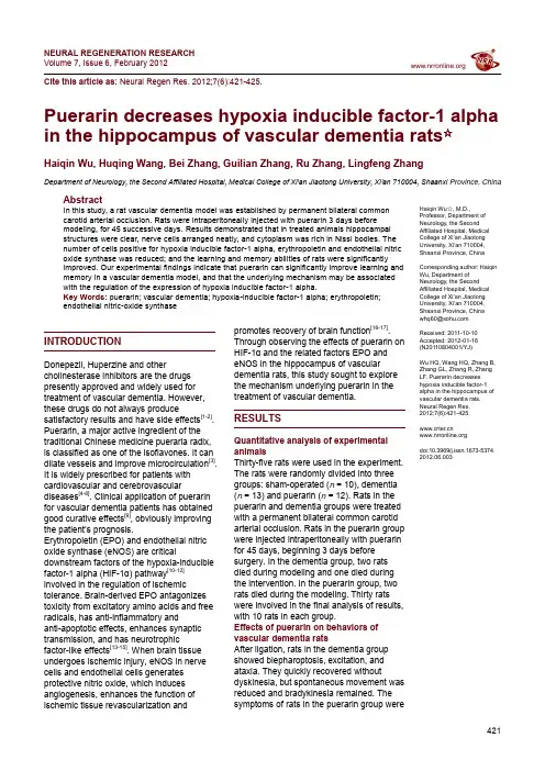
NEURAL REGENERATION RESEARCH Volume 7, Issue 6, February 2012Cite this article as: Neural Regen Res. 2012;7(6):421-425.421Haiqin Wu ☆, M.D.,Professor, Department of Neurology, the Second Affiliated Hospital, Medical College of Xi’an Jiaotong University, Xi’an 710004, Shaanxi Province, ChinaCorresponding author: Haiqin Wu, Department of Neurology, the Second Affiliated Hospital, Medical College of Xi’an Jiaotong University, Xi’an 710004, Shaanxi Province, China whq60@Received: 2011-10-10 Accepted: 2012-01-16 (N20110804001/YJ)Wu HQ, Wang HQ, Zhang B, Zhang GL, Zhang R, Zhang LF. Puerarin decreases hypoxia inducible factor-1 alpha in the hippocampus of vascular dementia rats. Neural Regen Res. 2012;7(6):421-425.doi:10.3969/j.issn.1673-5374.2012.06.003Puerarin decreases hypoxia inducible factor-1 alpha in the hippocampus of vascular dementia rats ☆Haiqin Wu, Huqing Wang, Bei Zhang, Guilian Zhang, Ru Zhang, Lingfeng ZhangDepartment of Neurology, the Second Affiliated Hospital, Medical College of Xi’an Jiaotong University, Xi’an 710004, Shaanxi Province, ChinaAbstractIn this study, a rat vascular dementia model was established by permanent bilateral common carotid arterial occlusion. Rats were intraperitoneally injected with puerarin 3 days before modeling, for 45 successive days. Results demonstrated that in treated animals hippocampal structures were clear, nerve cells arranged neatly, and cytoplasm was rich in Nissl bodies. The number of cells positive for hypoxia inducible factor-1 alpha, erythropoietin and endothelial nitric oxide synthase was reduced; and the learning and memory abilities of rats were significantly improved. Our experimental findings indicate that puerarin can significantly improve learning and memory in a vascular dementia model, and that the underlying mechanism may be associated with the regulation of the expression of hypoxia inducible factor-1 alpha.Key Words: puerarin; vascular dementia; hypoxia-inducible factor-1 alpha; erythropoietin; endothelial nitric-oxide synthaseINTRODUCTIONDonepezil, Huperzine and othercholinesterase inhibitors are the drugs presently approved and widely used for treatment of vascular dementia. However, these drugs do not always producesatisfactory results and have side effects [1-2]. Puerarin, a major active ingredient of the traditional Chinese medicine pueraria radix, is classified as one of the isoflavones. It can dilate vessels and improve microcirculation [3]. It is widely prescribed for patients with cardiovascular and cerebrovasculardiseases [4-8]. Clinical application of puerarin for vascular dementia patients has obtained good curative effects [9], obviously improving the patient’s prognosis.Erythropoietin (EPO) and endothelial nitric oxide synthase (eNOS) are criticaldownstream factors of the hypoxia-inducible factor-1 alpha (HIF-1α) pathway [10-12] involved in the regulation of ischemictolerance. Brain-derived EPO antagonizes toxicity from excitatory amino acids and free radicals, has anti-inflammatory andanti-apoptotic effects, enhances synaptic transmission, and has neurotrophicfactor-like effects [13-15]. When brain tissue undergoes ischemic injury, eNOS in nerve cells and endothelial cells generates protective nitric oxide, which induces angiogenesis, enhances the function of ischemic tissue revascularization andpromotes recovery of brain function [16-17]. Through observing the effects of puerarin on HIF-1α and the related factors EPO and eNOS in the hippocampus of vasculardementia rats, this study sought to explore the mechanism underlying puerarin in the treatment of vascular dementia.RESULTSQuantitative analysis of experimental animalsThirty-five rats were used in the experiment. The rats were randomly divided into three groups: sham-operated (n = 10), dementia (n = 13) and puerarin (n = 12). Rats in the puerarin and dementia groups were treated with a permanent bilateral common carotid arterial occlusion. Rats in the puerarin group were injected intraperitoneally with puerarin for 45 days, beginning 3 days before surgery. In the dementia group, two rats died during modeling and one died during the intervention. In the puerarin group, two rats died during the modeling. Thirty rats were involved in the final analysis of results, with 10 rats in each group.Effects of puerarin on behaviors of vascular dementia ratsAfter ligation, rats in the dementia group showed blepharoptosis, excitation, and ataxia. They quickly recovered withoutdyskinesia, but spontaneous movement was reduced and bradykinesia remained. The symptoms of rats in the puerarin group weremuch improved compared with those in the dementia group. There was no significant change in thesham-operated group before and after ligation. Puerarin enhanced the learning and memory abilities of vascular dementia ratsCompared with the sham-operated group, thelearning-memory scores of both the dementia and puerarin groups were significantly decreased 45 days after ligation of the common carotid arteries (P < 0.01). However, the puerarin group showed improvedlearning-memory scores compared with the dementia group (P < 0.05; Table 1).Puerarin ameliorated the hippocampal morphological changes in vascular dementia ratsIn the sham-operated group, light microscopy showed that hippocampal structures were clear, nerve cells were arranged regularly, and cytoplasm was rich in Nissl bodies. In contrast, in the dementia group, hippocampal structures were chaotic, nerve cells were enlarged and sparsely distributed, and cytoplasmic Nissl bodies were decreased or absent. In the puerarin group hippocampal structures were clearer than in the dementia group, nerve cells were regularly arranged and cytoplasm was rich in Nissl bodies (Figure 1). Puerarin inhibited the expression of HIF-1α, EPO and eNOS in the hippocampus of vascular dementia ratsImmunohistochemical staining showed that hippocampal tissues of all three groups expressed HIF-1α, EPO and eNOS. The immunoreactive products were stained brown. The positive cells were mainly distributed in the pyramidal cell layer in the CA1 region of the hippocampus, consistent with the characteristics of pyramidal cells (Figure 2). HIF-1α, EPO and eNOS positive cells in the CA1 region of the hippocampus were markedly increased in both the dementia and puerarin groups compared with thesham-operated group. Significant decreases in HIF-1α, EPO and eNOS positive cells were observed in the puerarin treated group compared with the control group (Table 2).Figure 1 Hippocampal morphology in rats from different groups (Nissl staining, × 400).(A) Sham-operated group: Hippocampal structures were clear, nerve cells arranged neatly, cytoplasm was rich in Nissl bodies.(B) Dementia group: Hippocampal structures were chaotic, nerve cells were enlarged and sparsely arranged, andNissl bodies decreased or disappeared.(C) Puerarin group: Hippocampal structures were clearer than in the dementia group. Neurons were neatly arranged and rich in cytoplasmic Nissl bodies.A B CFigure 2 Expression of hypoxia-inducible factor-1 alpha 1α), erythropoietin (EPO) and endothelial nitric-oxide422DISCUSSIONIn this study, a cerebral ischemia model was produced by occlusion of bilateral common carotid arteries. After ligation, rats in the dementia group showed blepharoptosis, excitation, and ataxia. They quickly recovered without dyskinesia, but spontaneous movement was reduced and bradykinesia remained. The learning-memory scores of the dementia group rats were markedly decreased in the Y-shaped water maze test. In the dementia group, hippocampal structures were chaotic; nerve cells were enlarged and arranged sparsely; and Nissl bodies in the cytoplasm were decreased or absent. Thus, this animal model, which is simple to prepare and shows features in line with clinical symptoms of vascular dementia, is an ideal model for studying vascular dementia.Puerarin is widely prescribed for patients with ischemic cardiovascular and cerebrovascular diseases. The therapeutic dose is 200-400 mg per day according to the description. There is no definite conclusion in the literature about the drug dose of puerarin for use in animal experiments. According to previously described findings[18-19] and our previous studies and preliminary experiments, we found that an intraperitoneal injection of 100 mg/kg was the optimal dose for treatment of vascular dementia rats. In the present study, the puerarin group remained healthy and demonstrated a better learning and memory performance than the dementia group. Histological examination showed a significant increase in the number of Nissl bodies, clear hippocampal structures, and significant changes in expression of HIF-1α, EPO and eNOS in the hippocampal CA1 region. Such structural and functional changes suggested that an intraperitoneal injection of 100 mg/kg puerarin is appropriate for vascular dementia in rats.Previous studies investigating the effects of puerarin on HIF-1α, EPO and eNOS of hypoxic-ischemic animals showed varied results. In the cerebralischemia-reperfusion model, Luo et al [18] found that the expression of EPO in cortex and basal ganglia in the cerebral ischemic-reperfusion rats was significantly increased after puerarin treatment. In contrast, results from Gu et al [19] showed that expression of eNOS in the brain tissue of rats with cerebral ischemia was decreased after puerarin treatment, but was still higher compared with the sham-operated group. In the rat model of myocardial infarction, Zhang et al[20] discovered that the expression of HIF-1 mRNA and eNOS mRNA in myocardial tissue in the puerarin group was significantly decreased. As reported by Wen et al [21], puerarin can elevate the level of eNOS protein and mRNA in myocardial cells. In this study, puerarin improved learning and memory, improved the hippocampal formation, and increased the intraneuronal Nissl bodies in vascular dementia rats, showing that it has protective effects against vascular dementia. Furthermore, in the hippocampal CA1 region, we observed the expression of HIF-1α, EPO and eNOS. Significantly more positive cells were present in the dementia group compared with the sham-operated group. The results indicated that HIF-1α, EPO and eNOS were closely related to vascular dementia. Following induction of vascular dementia, hippocampal neurons showed hypoxic-ischemic injury. HIF-1α was increased and played a role in self-protection by up-regulating the expression of EPO and eNOS which have neuroprotective effects. In this study, there were fewer positive cells in the puerarin group than in the dementia group, suggesting that puerarindown-regulated the expression of HIF-1α, EPO and eNOS in ischemic hippocampal CA1. This result is different from previous studies. We speculate that the possible causes are as follows: (1) Through increasing blood flow and improving cerebral microcirculation, puerarin improves hippocampal perfusion and increases oxygen concentration in nerve cells[7], thus negatively regulating the expression of HIF-1α and downstream protective factors EPO and eNOS. (2) Puerarin possesses an estrogen substitution effect[3, 22]. It is likely to increase tolerance of cells for hypoxia by acting at estrogen receptors, therefore down-regulating the expression of HIF-1α and t he downstream protective factors EPO and eNOS. Indeed, in this study puerarin down-regulated the expression of the protective HIF-1α pathway and downstream factors EPO and eNOS. Additionally, the learning and memory abilities of puerarin treated rats were significantly improved compared with the dementia group, but were still poorer than the sham-operated group. At the same time, there were fewer positive cells in the puerarin group than in the dementia group, but more than in the sham-operated group. This shows that puerarin can improve clinical symptoms of vascular dementia but cannot completely reverse the process of vascular dementia. Therefore, the most important thing is to prevent the occurrence of vascular dementia in clinic.Our study confirms that puerarin can improve clinical symptoms of vascular dementia and demonstrates that this action is associated with down-regulation of HIF-1α and its downstream factors, EPO and eNOS.423MATERIALS AND METHODSDesignA randomized, controlled animal experiment.Time and settingThe study was performed at the Medical College of Xi’an Jiaotong University, China from December 2009 to September 2010.MaterialsAnimalsA total of 35 male, specific pathogen freeSprague-Dawley rats, weighing 280 ± 20 g, aged 2- 3 months, were provided by the Experimental Animal Center of Medical School of Xi’an Jiaotong University, China (certificate No. SCXK (Shaan) 2007-001). Rats were housed on a 12-hour light/dark cycle, at 23.0 ±0.5°C and a relative humidity of 50.0 ± 0.5%, with free access to food and water. Animal procedures were in strict accordance with the Guidance Suggestions for the Care and Use of Laboratory Animals, issued by the Ministry of Science and Technology of China[23].DrugsPuerarin injection (4, 7-dihydroxy-8-β-D-glucosyl- isoflavone; Ankang Pharmaceutical Factory, Shaanxi, China; lot No. H20053144, 100 mg: 2 mL/bottle). The structure of puerarin is shown in Figure 3.MethodsEstablishment of vascular dementia rat models According to the methods described by de la Torre et al [24], rats in the puerarin group and dementia group were treated with a permanent bilateral common carotid arterial occlusion under anesthesia with peritoneal injection of 10% hydral chlorate (300 mg/kg). A longitudinal incision was made in the ventral neck to expose the common carotid arteries which were carefully dissected free from the vagus nerve and adjacent tissues. Then the common carotid artery was ligated with a silk suture. Animals assigned to the sham-operated group underwent the same surgical procedure without vessel occlusion. Puerarin interventionFrom 3 days before surgery, animals in the puerarin group were injected intraperitoneally with puerarin at a dose of 100 mg/kg per day for 45 days. Animals were injected 1 hour before ligation in the day of surgery. At the same time, animals in the sham-operated group and dementia group were injected intraperitoneally with 0.9% sodium chloride solution at a dose of 100 mg/kg.Y-type water maze test for detection of rat behavior The learning-memory abilities of rats were assessed in the Y-type water maze test[25]. The water maze consisted of a long arm (50 cm × 30 cm × 45 cm) and two short arms (40 cm × 30 cm × 45 cm). The long arm was the initiation region. One short arm was the blind zone (on the top of which there was an opaque plastic board, thereby decreasing the visibility of the canal); the other short arm was the safety zone with a platform of 30 cm ×10 cm and lamplight. Rats were trained over ten-trials. Their latency to arrive at safety zone from initiation region and the numbers of errors displayed by entering the blind zone were recorded as learning performances. After a 24-hour interval, the rats were tested again to obtain their memory performances. Before the experiment, the rats whose latency to arrive at safety zone were longer than 25 seconds were eliminated. After 45 days of intervention, the learning and memory abilities of the rats were once again evaluated with the Y-type water maze test.Collection of hippocampal samplesAfter 45 days of intervention, the rats were anesthetized, the chest was opened, the animals were perfused through the heart and the whole brain was removed. Brain tissues including hippocampus were then taken from coronal sections located from 3 mm after the bregma to the superior colliculus[26], and were paraformaldehyde fixed and paraffin-embedded.Nissl staining for cell morphology in the rat hippocampusThe hippocampal tissues were cut into 3-μm thick paraffin sections. They were deparaffinized with two changes of xylene for 15 minutes each, followed by 95% alcohol and 80% alcohol for 5 minutes each, then washed for 5 minutes with running water. The sections were next incubated in 1% toluidin blue (Tianyuan Biotechnology Co., Ltd., Shanghai, China) at 55°C for 30 minutes, and rinsed for 5 minutes. The sections were then rinsed with 80% alcohol, 90% alcohol, and 95% alcohol for 5 minutes each, then with three changes of xylene for 15 minutes each[27]. Last, the sections were mounted with neutral gum. The sections were observed under an optical microscope (B-type biomicroscope; Global Motic Group, Xiamen, China). Immunohistochemical staining for HIF-1α, EPO and eNOs expressionThe streptavidin-peroxidase immunohistochemical staining was executed in hippocampal tissues sections according to the kit instructions (Boster Biological Engineering Company, Wuhan, China). In brief, hippocampal tissue sections underwent dehydration through the ethanol gradient. The sections were treated with 3% H2O2 for 40 minutes at room temperature, microwave treated for 10 minutes for antigen retrieval, and cooled for 2 hours at room temperature. After incubation for 40 minutes in normal rabbit serum, they were incubated with primary antibodies, including rabbit anti-HIF-1α poly clonal antibody (1: 200; Boster Biological Engineering Company, Wuhan, China)[28], sheepanti-EPO multiclonal antibody (1: 500; Santa CruzFigure 3 Structure of puerarin.424Biotechnology, Delaware Santa Cruz, CA, USA)[29] and rabbit anti-eNOS polyclonal antibody (1: 100; Boster Biological Engineering Company)[19]. Subsequently, they were kept at 4°C overnight, treated with the biotinylated secondary antibodies, sheep anti rabbit IgG (HIF-1α, eNOS, 1: 200) or horse anti sheep IgG (EPO, 1: 500) for 40 minutes at room temperature, and incubated for30 minutes in streptavidin with horseradish peroxidase (1: 200) at room temperature. This was followed by DAB for 5 minutes, counterstaining with hematoxylin, dehydration, and coverslipping. Negative control sections were treated with TBS instead of primary antibody.Six sections from each group were observed under an optical microscope. The positive cells were nerve cells in hippocampus showing buffy granules. The data were expressed as the mean of number of positive cells/mm2 in five random high-power fields (400 × magnification) from the CA1 region of the hippocampus.Statistical analysisData were analyzed using SPSS 12.0 software (SPSS, Chicago, IL, USA) and a level of P < 0.05 was assessed as a statistically significant difference. All values in the figures of present study indicate mean ± SD. Group comparisons were analyzed with analysis of two-sample t-test.Author contributions: Haiqin Wu designed this study and revised the manuscript. Huqing Wang and Bei Zhang provided experimental data, participated in statistical analysis and wrote the manuscript. Guilian Zhang and Ru Zhang provided technical support and statistical calculations. Lingfeng Zhang provided information support.Conflicts of interest:None declared.Ethical approval:This study had the approval of the Animals Ethics Committee of Medical College of Xi’an Jiaotong University in China.Acknowledgments:We would like to thank Ming Li, from Department of Anatomy, Medical College of Xi’an Jiaotong University, China for technical support.REFERENCES[1] Román GC, Salloway S, Black SE, et al. Randomized,placebo-controlled, clinical trial of donepezil in vascular dementia: differential effects by hippocampal size. Stroke. 2010;41(6):1213-1221.[2] Wilkinson D, Róman G, Salloway S, et al. The long-term efficacyand tolerability of donepezil in patients with vascular dementia. Int J Geriatr Psychiatry. 2010;25(3):305-313.[3] Yin LH, Li YF, Meng FL. Puerarin's chemical compositionpharmacological effects and clinical application. HeilongjiangYiyao. 2010;23(3):371-373.[4] Sun GH. A review on the clinical application of Puerarin. ZhongyiLinchuang Yanjiu. 2010;2(6):100-101.[5] Ji AL, Zhang XJ. Effect of puerarin injection on inflammatoryfactors in patients with acute cerebral infarction. NanjingZhongyiyao Daxue Xuebao: Ziran Kexue Ban. 2009;25(2):145-147.[6] Yao PF, Fan HX, Qian YL. Study of puerarin injection on acuteischemic brain infarction in the aged. Xiandai Zhongxiyi JieheZazhi. 2009;18(14):1587-1590. [7] Yu WH, Chu GL. Researching development of the protectiveeffects of puerarin in hypoxic ischemic brain damage. YixueZongshu. 2009;15(20):3163-3165.[8] Zhang R, Cheng HX, Wu HQ, et al. Effect of Puerarin on nNOSexpression in hippocampal neurons after focal cerebral ischemiain rats. Xi'an Jiaotong Daxue Xuebao: Yixue Ban. 2010;31(6):669-672.[9] Zhang T, Zhang XQ, Zhu RH. The report of puerarin and citicolinein 36 cases with vascular dementia. Shandong Zhongyiyao Daxue Xuebao. 2000;24(1):37-38.[10] Semenza GL. HIF-1: upstream and downstream of cancermetabolism. Curr Opin Genet Dev. 2010;20(1):51-56.[11] Corzo CA, Condamine T, Lu L, et al. HIF-1α regulates functionand differentiation of myeloid-derived suppressor cells in thetumor microenvironment. J Exp Med. 2010;207(11):2439-2453. [12] Takubo K, Goda N, Yamada W, et al. Regulation of the HIF-1alphalevel is essential for hematopoietic stem cells. Cell Stem Cell.2010;7(3):391-402.[13] Noguchi CT, Asavaritikrai P, Teng R, et al. Role of erythropoietin inthe brain. Crit Rev Oncol Hematol. 2007;64(2):159-171.[14] Zhang F, Xing J, Liou AK, et al. Enhanced delivery oferythropoietin across the blood-brain barrier for neuroprotectionagainst ischemic neuronal Injury. Transl Stroke Res. 2010;1(2):113-121.[15] Genc K, Egrilmez MY, Genc S. Erythropoietin induces nucleartranslocation of Nrf2 and heme oxygenase-1 expression inSH-SY5Y cells. Cell Biochem Funct. 2010;28(3):197-201.[16] Ito Y, Ohkubo T, Asano Y, et al. Nitric oxide production duringcerebral ischemia and reperfusion in eNOS- and nNOS-knockoutmice. Curr Neurovasc Res. 2010;7(1):23-31.[17] Aoki T, Nishimura M, Kataoka H, et al. Complementary inhibitionof cerebral aneurysm formation by eNOS and nNOS. Lab Invest.2011;91(4):619-626.[18] Luo YM, Gao L, Ji XM, et al. Effects of puerarin on EPOexpressions in ischemic brain tissues of rats following MCAO.Zhongguo Laonian Xue Zazhi. 2008;28(12):1057-1059.[19] Gu CZ, Lu HL, Wu QH, et al. The effects of puerarin on theepression of eNOS in brain tissues after cerebral ischemiareperfusion in rats. Zuzhong yu Shenjing Jibing. 2010;17(6):336-338.[20] Zhang SY, Shen YJ, Chen SL, et al. The effects of puerarin onHIF-1, eNOS, VEGF genes expressions in myocardium and NO in serum of rats with myocardial infarction. Zhongyi Yaoli yuLinchuang. 2007;23(5):54-57.[21] Wen J, Chen SL, Filly C, et al. Effect of puerarin on nitric oxideproduction in H9C2 cells. Zhongguo Xinxueguan Bing Zazhi.2006;4(10):777-779.[22] Huang T, Jin BQ, Sun GJ, et al. Effects of puerarin on the bonemetabolism in ovariectomized rats. Zhongguo Laonian Xue Zazhi.2009;29(19):2482-2484.[23] The Ministry of Science and Technology of the People’s Republicof China. Guidance Suggestions for the Care and Use ofLaboratory Animals. 2006-09-30.[24] de la Torre JC, Fortin T, Park GA, et al. Chronic cerebrovascularinsufficiency induces dementia-like deficits in aged rats. Brain Res.1992;582(2):186-195.[25] Wang CF, Li DQ, Xue HY, et al. Oral supplementation of catalpolameliorates diabetic encephalopathy in rats. Brain Res. 2010;1307:158-165.[26] Paxinos G, Watson C. The Rat Brain in Stereotaxic Coordinates.5th ed. London: Academic Press. 2005.[27] Yu SS, Zhao J, Zheng WP, et al. Neuroprotective effect of4-hydroxybenzyl alcohol against transient focal cerebral ischemiavia anti-apoptosis in rats. Brain Res. 2010;1308:167-175.[28] Peng Z, Ren P, Kang Z, et al. Up-regulated HIF-1alpha is involvedin the hypoxic tolerance induced by hyperbaric oxygenpreconditioning. Brain Res. 2008;1212:71-78.[29] Wu H, Wang H, Sha J, et al. Expression of hypoxia induciblefactor-1alpha and erythropoietin in the hippocampus of aging rats.Zhong Nan Da Xue Xue Bao Yi Xue Ban. 2009;34(9):856-860.(Edited by Wang XD, Shi ZH/Yang Y/Wang L)425。

微生物细胞脂肪酸的组成分析柳志杰;章辉;周利;花强【摘要】The composition of microorganism cellular fatty acid was analyzed by gas chromatography-mass spectrometry (GC-MS). The results showed that the metabolism of the strain could be divided into cell growth stage and fatty acid accumulation stage. T. Cutaneum lipid was mainly comprised of oleic acid(C18 :1) ,palmitic acid(C16:0) ,palmitoleic acid(C16:l). The fatty acid composition was as follows: oleic acid(C18:1)64. 80%, palmitic acid(C16: 0)19. 90%, palmitoleic acid(C16 : 1) 10.94% , stearic acid (C18: 0) 3. 72% and linoleic acid (C18:2)0. 56% ,respectively. The fatty acid methyl esters could be well analyzed by GC-MS, which could also be generalized to many other applications.%应用气相色谱—质谱联用技术(GC-MS)对微生物细胞脂肪酸的组成进行了分析.结果表明,菌体的代谢状态分为两个时期:菌体生长期和油脂积累期；菌体细胞主要积累油酸(C18:1)、软脂酸(C16:0)和棕桐油酸(C16:1);通过发酵,最终得到的微生物油脂脂肪酸组成为:油酸(C18:1)64.80％、软脂酸(C16:0)19.90％、棕桐油酸(C16:1)10.94％、硬脂酸(C18:0)3.72％和亚油酸(C18:2)0.56％.GC-MS可以很好地用于脂肪酸甲酯的分析,具有普遍的应用意义.【期刊名称】《化学与生物工程》【年(卷),期】2011(028)010【总页数】3页(P85-87)【关键词】微生物细胞;油脂含量;脂肪酸组成;气相色谱—质谱联用技术【作者】柳志杰;章辉;周利;花强【作者单位】华东理工大学生物反应器工程国家重点实验室,上海200237;华东理工大学生物反应器工程国家重点实验室,上海200237;华东理工大学生物反应器工程国家重点实验室,上海200237;华东理工大学生物反应器工程国家重点实验室,上海200237【正文语种】中文【中图分类】O657.7微生物油脂又称单细胞油脂，是微生物在一定条件下产生并储存于菌体内的甘油脂，其脂肪酸组成以C16、C18系脂肪酸(如硬脂酸、油酸和亚油酸)为主。

河南省创新发展联盟2024-2025学年高三上学期9月月考英语试题一、阅读理解Join a Zion National Park ranger (护林人) to learn about what makes Zion National Park unique. Programs are free and created for classrooms and individuals. We connect to your school or home through a free web-based program. You will be provided with a link to the video conference ahead of time via an email invite. Registration is open! Click on the program below for more information. Program 1—Chat with a RangerIn Chat with a Ranger, students learn about Zion National Park, the park service, and the life of a ranger. Students prepare and send questions ahead of time. This program can be adapted to fit different curriculum objectives, and is appropriate for any age group. Program 2—Pollination InvestigationIn this distance learning program, students will discover what pollination is and how important it is to all ecosystems. Looking at the relationship between plants and pollinators, participants will see how they have influenced each other and will be challenged to create their own perfect pollinator. Program 3—Whooo’s in the Canyon?Who left these clues behind here in the high canyons of Zion National Park? A feather, small bones, and hoot hooting in the trees can be heard as your classroom goes on a virtual hike of Zion to discover the Mexican spotted owl. Learn it about how the owl uses its special adaptations to survive in this desert environment. Program 4—The Forests, Wetlands, and Deserts of Zion This distance learning program focuses on the plants and animals that live in Zion's varying ecosystems. Students will learn about their adaptations and relationships to each other in this interactive lesson with a creative and critical thinking activity.1．Which program requires participants to make preparations in advance?A．Chat with a Ranger.B．Pollination Investigation.C．Whooo's in the Canyon?D．The Forests, Wetlands, and Deserts of Zion. 2．What can participants learn from program 3?A．Survival strategies taken by owls in the park.B．Ways to prepare a hike tour in the park.C．Threats brought by the desert environment.D．A variety of ecosystems in ZionNational Park.3．What do the listed programs have in common?A．They involve interactive activities.B．They include a virtual tour of different trails.C．They are accessible through web-based program.D．They require participants to visit the park in person.On a hot June day in 2015, I retired after 34 years of teaching high school. Then, I drove to meet my new piano teacher, Mark.I had worked for more than three decades as a busy English teacher with an endless stream of papers to mark and precious little time to experiment or learn new skills. I was determined to make up for all I had been missing. I wanted to finally master the piano and learn how to make music.I told Mark I had a specific concrete goal: to play Clair de lune by Claude Debussy, a piece I remember hearing from early childhood.Determined that there would be a day when I would totally master this piece, I set myself a deadline: I would perform before a gathering of friends on my 60th birthday. For months I did nothing but furiously (猛烈地) practise. When the day came, around 30 friends and relatives crowded into my dining room to hear me play, and aside from a few minor slips, I managed to pull it off without embarrassing myself. People clapped warmly. I made it. I had risen to a challenge, but I still didn’t feel that I was really “making music”.After that, my progress was painfully slow. I had come to hate hearing myself play music badly. I got no pleasure from the act of missing notes.I began focusing on what few things I could do: gardening and cycling. I came to understand that I didn’t have to be that man I’d always thought I ought to be. I could just do what feels good. So, after nearly five years of lessons, I quit.I still love music; I regularly go out to concerts. But now my piano does nothing more than sit silently in my dining room, displaying family photos and collecting dust. And I’m perfectly happy with that.4．Why did the author learn the piano after retiring from teaching?A．To impress his friends and relatives.B．To avoid the boredom of retirement.C．To start a new career as a concert pianist.D．To pursue a long-time passion for music. 5．What can be inferred from paragraph 4?A．The author attended a concert of piano music.B．The author performed successfully despite a few errors.C．The author felt embarrassed about his piano performance.D．The author quit his piano immediately after his 60th birthday.6．What does the author do with his piano now?A．He uses it for music lessons.B．He uses it for performance.C．He uses it for something unrelated to music.D．He plays it for personal enjoyment occasionally.7．Which of the following can best describe the author?A．Inner- directed and hardworking.B．Conventional and careless.C．Ambitious and kind-hearted.D．Lazy and pessimistic.When it comes to diatoms (硅藻类) that live in the ocean, new research suggests that photosynthesis (光合作用) is not the only strategy for accumulating carbon. Instead, these single-celled are also building biomass by feeding directly on organic carbon in the ocean.These new findings could lead researchers to reduce their estimate of how much carbon dioxide diatoms pull out of the air via photosynthesis, which in turn, could take a much closer look at the understanding of the global carbon cycle, which is especially relevant given the changing climate. The new findings were published in Science Advances on July 17, 2024.The team showed that the diatom Cylindrotheca closterium, which is found in oceans around the world, regularly performs a mix of both photosynthesis and direct eating of carbon from organic sources such as plankton (浮游生物) . In more than 70% of the water samples the researchers analyzed from oceans around the world, the team found signs of simultaneous photosynthesis and direct organic carbon consumption from Cylindrotheca closterium. The team also showed that this diatom species can grow much faster when consuming organic carbon in addition to photosynthesis. Furthermore, the new research hinted at the possibility that specificspecies of bacteria are feeding organic carbon directly to a large percentage of these diatoms living all across the global ocean. This work is based on a genome-scale metabolic modeling approach that the team used to reveal the metabolism of the diatom Cylindrotheca closterium.The team’s new metabolic modeling data support recent lab experiments suggesting that some diatoms may rely on strategies other than photosynthesis to intake the carbon they need to survive, thrive and build biomass.The UC San Diego led team is in the process of expanding the scope of the project to determine how widespread this non-photosynthetic activity is among other diatom species. 8．What’s new according to the research?A．The way of the diatom’s carbon accumulation.B．The impact of climate on diverse sea plants.C．The procedure of exploring carbon.D．The system of building biomass.9．What do the new findings make researchers more focus on?A．The causes of climate change.B．The grasp of the carbon cycle.C．The bad effect of photosynthesis on diatoms.D．A rough estimate of the amount of carbon dioxide.10．What do we know from paragraph 3?A．A large number of diatoms may feed on bacteria.B．The diatom lives on plankton.C．Water samples are key factors for the research.D．Diatom species grow faster with sufficient sunlight11．Which is the most suitable title for the text?A．Photosynthesis in Diatoms B．Plankton’s Role in OceansC．New Carbon Strategies in Diatoms D．Advances in Modeling DataAccording to a report in 2023, the World Health Organization (WHO) recommended that non-sugar sweeteners not be used as a means of achieving weight control or reducing the risk of diseases. The guideline came as a surprise. After all, the very purpose of non-sugar sweeteners-which contain little to no calories—is to help consumers control their weight and reduce their risk of disease by replacing sugar.In its report, the WHO cited evidence that long-term use of non-sugar sweeteners is associated with an increased risk of diabetes (糖尿病) and death. How is it that non-sugar sweeteners are linked to the negative health effects they’re supposed to fend off?The WHO made its recommendation after reviewing hundreds of published studies. The problem is that the overwhelming majority of these studies are observational. In such studies, subjects tend to self-report their food intake, which might not guarantee inaccuracy. More importantly, observational studies cannot determine cause and effect. Are non-sugar sweeteners causing diabetes, or are people at risk of diabetes simply more likely to consume them? Lastly, there are numerous variables that researchers can’t possibly control for in these studies that could influence the results.Randomized controlled trials (RCTs) tell a different story about non-sugar sweeteners. These studies control for variables by randomly assigning people to either a treatment or control group, and they can determine cause and effect. They show that sweeteners modestly benefit weight loss and help control blood sugar, without the negative effects seen in observational research. The downside of RCTs is that they are shorter in duration, often lasting just a few months. So negative effects could appear after longer use and we wouldn’t be able to tell from these RCTs.But we also can’t tell from observational studies, which only measure correlation and not causality (因果关系) . Changing the current situation might be hard, though. RCTs are expensive and require recruiting participants, setting up diet plans, and regularly measuring subjects’ health outcomes.For change to happen, it might need to start at the top, where science is funded Government agencies, which appropriate billions for research, should start prioritizing RCTs.12．What do the underlined phrase “fend off” probably mean in paragraph 2?A．Put out.B．Defend against.C．Keep up.D．Count on. 13．What does paragraph 3 mainly talk about?A．The WHO’s suggestions on observational studies.B．The strategies to decide cause and effect in conducting studies.C．The significance of controlling variables in observational studies.D．The limitations of the observational studies in the WHO report.14．What is a feature of RCTs according to the text?A．They cost little B．They tend to last long.C．They can control variables and determine causality.D．They require participants to self-report related data15．How should the government help RCTs?A．By making appropriate plans B．By providing financial supportC．By raising people’s awareness of health D．By founding more related governmentagenciesTo make science’s stories more concrete and engaging, it’s important to use some effective strategies. Here are four of them. Put people in the storyScience’s stories often lack human characters. 16 . Characters can be also people affected by a scientific topic, or interested in learning more about it. Besides, they can be storytellers who are sharing their personal experiences.17People often think of science as objective and fair. But science is actually a human practice that continuously involves choices, missteps and biases (偏见) . If you explain science as a course, you can walk people through the sequence of how science is done and why researchers reach certain conclusions. 18 . And they can also stress the reason why people should trust the course of science to provide the most accurate conclusions possible given the available information. Include what people care aboutScientific topics are important, but they may not always be the public’s most pressing concerns. In April 2024, a polling company found that “the quality of the environment” was one of thelowest-ranked priorities among people in the US. The stories about the environment could weave in connections to higher-priority topics. 19 . Tell science's storiesScientists, of course, can be science communicators, but everyone can tell science’s stories. When we share information online about health, or talk to friends and family about the weather, we contribute to information that circulates about science topics. 20 . Think about all of a story’s characteristics - character, action, sequence, scope, storyteller and content - and how you might incorporate them into the topic.A．Explain science as a processB．Shoot attractive short science videosC．Scientists themselves can actually become ideal onesD．This practice is to stress why the content is importantE．You can tell growth stories of remarkable teenage scientistsF．Science communicators can emphasize how science is conductedG．You may as well borrow features from stories to strengthen your message二、完形填空In 2018, Molly Baker unfortunately lost her husband in a severe skiing accident. She was 21 . In the first several weeks after his passing, her friends and family 22 a great deal of support. But after a while, the cards and meals started to 23 . “People had to get back to their normal 24 . And so things kind of dropped off,” Baker recalled.That was when one of Baker's friends, Carla Vail, thought up a way to 25 the help for an entire year. She called it the “Calendar Girls”. V ail gathered the names of 31 of Baker's friends who wanted to help, and 26 each friend a particular day. Vail also gave Baker the names on the 27 , so Baker could know what to 28 each day.“And what that looked like for them was that on that day, they would reach out to me in some 29 ways—maybe via text, or a card,” Baker said.Looking back, Baker feels that Vail's 30 was essential to helping her cope with her husband's death, because she was 31 at that time.“A lot of people are really uncomfortable around 32 ,” Baker said. “So what they do is, instead of doing something, that they 33 do nothing. It was nice to have that ‘Calendar Girls’ setup.”Today, Baker tries to do something similar for her friends going through 34 . In hard times, she knows how 35 it is to have something to look forward to every day. 21．A．cautious B．unconscious C．desperate D．impassive 22．A．extended B．demanded C．announced D．assumed 23．A．pass down B．show up C．break up D．slow down24．A．exercise B．routine C．diet D．growth 25．A．resist B．continue C．explain D．test 26．A．ordered B．sent C．owed D．assigned 27．A．furniture B．file C．calendar D．Internet 28．A．expect B．absorb C．propose D．define 29．A．rare B．strange C．specific D．generous 30．A．curiosity B．thoughtfulness C．ambition D．toughness 31．A．innocent B．optimistic C．tolerant D．lonely 32．A．panic B．evidence C．failure D．grief 33．A．simply B．hardly C．skillfully D．secretly 34．A．distraction B．addiction C．loss D．annoyance 35．A．amusing B．valuable C．astonishing D．universal三、语法填空阅读下面短文，在空白处填入1个适当的单词或括号内单词的正确形式。

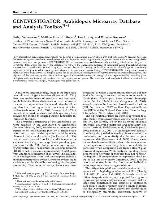
BioinformaticsGENEVESTIGATOR.Arabidopsis Microarray Database and Analysis Toolbox1[w]Philip Zimmermann2,Matthias Hirsch-Hoffmann2,Lars Hennig,and Wilhelm Gruissem*Institute of Plant Sciences,Swiss Federal Institute of Technology and Zurich-Basel Plant ScienceCenter,ETH Center,CH–8092Zurich,Switzerland(P.Z.,M.H.-H.,L.H.,W.G.);and Functionaland Genomics Center Zurich,UNI Irchel,Y32H52,CH–8057Zurich,Switzerland(W.G.)High-throughput gene expression analysis has become a frequent and powerful research tool in biology.At present,however, few software applications have been developed for biologists to query large microarray gene expression databases using a Web-browser interface.We present GENEVESTIGATOR,a database and Web-browser data mining interface for Affymetrix GeneChip ers can query the database to retrieve the expression patterns of individual genes throughout chosen environmental conditions,growth stages,or organs.Reversely,mining tools allow users to identify genes specifically expressed during selected stresses,growth stages,or in particular ing GENEVESTIGATOR,the gene expression profiles of more than22,000Arabidopsis genes can be obtained,including those of10,600currently uncharacterized genes.The objective of this software application is to direct gene functional discovery and design of new experiments by providing plant biologists with contextual information on the expression of genes.The database and analysis toolbox is available as a community resource at https://www.genevestigator.ethz.ch.A major challenge in biology today is the large-scale determination of gene function(Boyes et al.,2001). First,the establishment of standards and controlled vocabularies facilitates the integration of experimental data into a computational framework,thereby allow-ing structured and systematic processing of infor-mation(Ashburner et al.,2000;Brazma et al.,2001). Second,structured databases and data querying tools provide the means to assign putative functional in-formation to genes.The complete sequencing of the Arabidopsis ge-nome achieved in the year2000(The Arabidopsis Genome Initiative,2000)enables us to monitor gene expression of thisflowering plant on a genome-scale using microarrays.In situ synthesis of high-density oligonucleotides on glass slides(Lockhart et al.,1996) has become a powerful tool to rapidly integrate the sequence knowledge into expression profiling plat-forms,such as the ATH1full genome array developed by Affymetrix and The Institute for Genomic Research (TIGR),which represents approximately23,750genes from Arabidopsis(Redman et al.,2004).The availabil-ity of a full-genome array and the complete technical environment provided by the Affymetrix system led to a wide use of the GeneChip technology in the plant community.Thousands of arrays have since been processed,of which a significant number are publicly available through services and repositories such as Nottingham Arabidopsis Stock Centre Transcrip-tomics Service(NASCArrays;Craigon et al.,2004), ArrayExpress at the European Bioinformatics Institute (EBI;Brazma et al.,2003),or Gene Expression Omni-bus(GEO)at the National Center for Biotechnology Information(NCBI;Edgar et al.,2002).The exploitation of large-scale gene expression data-sets,mainly from Saccharomyces cerevisiae and Escheri-chia coli,has already led to the discovery of global structures governing metabolic and regulatory net-works(Lee et al.,2002;Ravasz et al.,2002;Stelling et al., 2002;Ihmels et al.,2004).Multiple-genome compar-isons have also yielded interesting observations on the modularity and connectivity distributions of gene expression data(Bergmann et al.,2004).Nevertheless, the combination of multiple datasets still raises a num-ber of questions concerning their compatibility,in particular when comparing data from different plat-forms and organisms.While analyses revealing global properties of networks or modules may not necessar-ily require full compatibility of expression datasets, the details are often noisy(Friedman,2004)and the comparative search for the function of individual genes requires a more stringent selection.The Affymetrix platform provides a standardized system with a high degree of reproducibility(Hennig et al.,2003;Redman et al.,2004).Although data from different experiments may not be pooled for a rigorous expression profiling analysis,one can assume that the large-scale combination and analysis of expression data from a single organism using a single platform like the Affymetrix system allows the identification of biologically meaningful expression patterns of1This work was supported by ETH,Strategic Excellence Project 2–74213–02/TH–8/02–2,and by the Functional Genomics Center Zurich.2These authors contributed equally to the paper.*Corresponding author;e-mail wilhelm.gruissem@ipw.biol. ethz.ch;fax41–1–632–10–79.[w]The online version of this article contains Web-only data./cgi/doi/10.1104/pp.104.046367.individual genes.To date,few tools have been de-veloped for biologists to query large gene expression databases.The Yeast Microarray Global Viewer (yMGV)is a database providing online tools for the analysis of transcriptional expression profiles of yeast genes among82different datasets(Lelandais et al., 2004).In the plant community,NASCArrays(Craigon et al.,2004)provides a repository for Arabidopsis microarray data and some simple‘‘gene-centric’’data mining tools.Here,we describe a novel online tool called GENEVESTIGATOR comprising a gene expression database and a number of querying and analysis functionalities developed to facilitate gene functional discovery.GENEVESTIGATOR allows the data to be presented in the context of plant development,plant organ,and environmental conditions,both for indi-vidual genes or for families of genes,thereby answer-ing questions such as‘‘in which growth stage is my gene of interest expressed?’’or‘‘which genes are specifically expressed in roots?’’The main objective of the software is to assign contextual information togene expression data,directing the design of new experiments and gene functional discovery.RESULTSDatabase Concept and Software Design GENEVESTIGATOR was conceived as a user-friendly online tool for large-scale expression data analysis.It consists of a MySQL relational database and a Web server application programmed in the PHP (PHP Hypertext Preprocessor)scripting language.The database works as a‘‘data warehouse’’containing experimental and annotation data,preprocessed data, as well as diverse tables for control of workflow and analysis(Fig.1).Raw experimental data from users is processed using Affymetrix MAS5.0software to a target value (TGT)of1,000(Liu et al.,2002).Signal intensities and P values are collected for each hybridized Affymetrix GeneChip array.Alternatively,data and annotation can be imported from public repositories such as ArrayExpress(Brazma et al.,2003)and GEO(Edgar et al.,2002).The assignment of array elements(probe sets)to Arabidopsis locus identifiers(AGI codes)and their annotations is based on regularly updated data-sets obtained from the Arabidopsis Information Re-source(TAIR)ftp server(ftp:/// home/tair/Microarrays/Affymetrix/;currently as of April5,2004,based on thefinal Arabidopsis genome annotation release from TIGR[version5.0,January 2004]).In addition to probe sets representing unique genes(ending‘‘_at’’),the ATH1and AG GeneChip arrays include nonunique probe sets representing two or more closely related genes(ending‘‘_s_at’’)or multiple cross-hybridizing probe sets(ending ‘‘_x_at’’;for details,see Redman et al.,2004).Although these probe set types represent two or more genes, only one locus identifier is displayed per probe set. These ambiguous probe sets are highlighted in GENEVESTIGATOR to draw the attention of the user to this issue.The experiment annotation is curated,entered,and structured in either hierarchical(e.g.plant organs), unique(e.g.growth stage),or multi-select form(e.g. environmental condition).The software has been de-signed for easy additions of new annotations in any of these formats and for rapid creation of the correspond-ing tools to analyze and visualize the data.The annotation of arrays was based on the information provided by users or public repositories.Missing information does not impact the results,as the corre-sponding arrays are not included into the respective calculations.Ambiguous or unsuitable annotations were further ignored.For example,arrays from RNA extracted from whole adult plants(including roots, rosette leaves,and inflorescence)are unsuitable for tools relating to plant organ specificity(Gene Atlas) and are therefore not included into the corresponding calculations,but may be proper for use in other tools such as Gene Chronologer.Each tool therefore accesses the best respective available sources of data for pro-cessing,while unsuitable data is ignored.Data from the ATH1and AG arrays are processed separately.Different sets of oligonucleotide sequences are used to probe identical target genes on the two array types,and thus different efficiencies of target to probe hybridization and nontarget to probe cross-hybridization makes a direct comparison of signal intensities impossible.Although a high degree of re-producibility was found for most target genes probed by both the ATH1and the AG arrays,300pairs of probe set for identical target genes yielded strongly differing results(Hennig et al.,2003).Figure 1.Concept and design of GENEVESTIGATOR.The experi-menter submits RNA profiling data to the database curator,who processes the data and uploads it to the database.The datawarehouse contains raw signal intensity and P values,as well as preprocessed tables.A Webserver application acts as an interface between users and the GENEVESTIGATOR database.Zimmermann et al.As of July2004,the database contained publicly available data from750ATH1and121AG arrays covering81public experiments from the Gruissem Laboratory(http://www.pb.ethz.ch;Menges et al., 2003;Hennig et al.,2004;Kleffmann et al., 2004),the Functional Genomics Center Zurich (http://www.fgcz.ethz.ch),NASCArrays(http:// /narrays/experimentbrowse. pl;Craigon et al.,2004),ArrayExpress at EBI(http:// /arrayexpress/;Brazma et al.,2003), and from GEO at NCBI(http://www.ncbi.nlm.nih. gov/geo/;Edgar et al.,2002). GENEVESTIGATOR is freely accessible to all aca-demic institutions.Since the database contains at present both publicly available as well as confidential data,we have implemented a dual user profile management system for public and private users. All users are therefore asked to register once and to login for each session.We limit the collection and use of personal information to what is necessary to administer the database and improve the utility of GENEVESTIGATOR.Personal information is not shared with third parties.Analysis ToolsThe GENEVESTIGATOR tools generally contain two types of queries:a gene-centric approach report-ing signal intensity values for individual genes,and a genome-centric approach providing lists of genes fulfilling chosen criteria.The results obtained from any tool are based on all available signal intensity values and the corresponding annotations.In some cases,present/absent call information as defined by the MAS5.0algorithm is indicated(see below).Thefirst tool,Digital Northern,will retrieve the signal intensity values of input genes for a chosen selection of GeneChip experiments.An elaborate se-lection tool(Fig.2A)allows the user to choose exactly those experiments thatfit single or multiple criteria such as anatomy,growth stage,or environmental factors.Up to10probe sets can be processed simul-taneously,displayed in several colors,shapes,and filling,revealing both signal intensity values and present call(closed symbols)and absent call(open symbols)information(Fig.2B).The Gene Correlator allows comparing the signal intensity values of two genes throughout all chosen experiments(Fig.2C;identical selection tool as for Digital Northern).Each spot represents a GeneChip and can be identified by mouse-over or by linking to the annotation database.The Pearson’s correlation coefficient is given as a measure for the relationship between expression signals of two genes.Present call information is visualized by a color coding(Fig.2C). Because the objective of the software was to provide contextual information for the expression of genes,we additionally focused on relating gene expression to three main annotation groups:plant organ,develop-mental stage,and environmental stress.The Gene Atlas tool similarly provides the average signal intensity values of a gene of interest in all organs or tissues annotated in the database(Fig.2D).Re-versely,GENEVESTIGATOR can output lists of genes for which signal intensities exceed a chosen threshold in selected organs versus a baseline choice of organs (Fig.2E).This allows users tofind genes expressed preferentially in certain organs or tissues,such as roots,young leaves or stamina.The anatomy annota-tion was based on standard anatomy terms as defined by the Plant Ontology Consortium(/)that we classified into six main groups (callus,cell suspension,seedling,inflorescence,ro-sette,and roots)and the corresponding subgroups. These categories cover all tissues that can currently be isolated for expression analysis,but can easily be extended as tissue and cell separation techniques become more precise(Birnbaum et al.,2003).The Gene Chronologer tool,based on the Boyes growth stage ontology(Boyes et al.,2001),possesses two main features.First,it outputs the average signal intensities(or expression levels)and SE s of a gene of interest for10representative sections of the life cycle of Arabidopsis(Fig.2F).Second,users can query the database to output all genes expressed above a given threshold at chosen growth stages.For example,all genes can be selected for which the signal intensity at the seedling stage exceeds90%of the sum of all average signal intensity values for each category,measured for this gene throughout the life cycle of the plant(Fig.2G).The Response Viewer tool provides the same func-tionalities as Gene Atlas and Gene Chronologer,based on stress response annotations(Fig.2,H and I).For each condition,one or several representative experi-ments were chosen.Each stress factor is given with the corresponding control from these experiments,allow-ing direct comparison.The Meta-Analyzer utility has been designed to study the gene expression profiles of several genes simultaneously in the context of environmental stresses,organs,and growth stages(Fig.2,J–L).Lists of genes can be entered in diverse formats(comma-, semi-colon-,or space-separated,CRLF[carriage re-turn,line feed],or directly copied from a spreadsheet). The output is a heat map of normalized signal in-tensity values(see Documentation section on our Web page)clustered by either single,average,or complete linkage hierarchical clustering.This tool is especially useful to compare members of gene families and to identify clusters of similarly expressed genes. Finally,the Database and Documentation sections provide users with annotation information about ex-periments in the database,as well as technical infor-mation(Fig.2,M and N).Since GENEVESTIGATOR was conceived to be an analysis tool and not a data repository,a reduced set of annotations is stored locally. The full MIAME(Minimum Information About a Microarray Experiment)compliant annotations (Brazma et al.,2001)are available by linking to theGENEVESTIGATORZimmermann et al.Figure2.Screenshots of some of the features of GENEVESTIGATOR.Top left,Logo and available tools.A,Chip Selection tool;B, Digital Northern;C,Gene Correlator;D and E,Gene Atlas(relates to plant anatomy);F and G,Gene Chronologer(relates to the plant growth stages);H and I,Response Viewer(relates to environmental factors);J to L,Meta-Analyzer(multiple gene analysis with respect to anatomy,growth stage,and environmental factors);M and N,Database tool for viewing experiment and array annotation,and Documentation section for user information.corresponding repository sites from which the experi-ments were downloaded.General Approach and ValidationThe database contains expression data from a high diversity of experiments covering different tissues,ages,and treatments (Table I).The general hypothesis in our approach is that as the number of experiments per category (e.g.growth stage 5.10)increases,in-dividual effects are averaged out and global trends become visible.As a measure of confidence for the expression of genes in different categories,we indicate the respective number of GeneChips and the SE of the mean for each category.To validate our hypothesis,we checked whether strongly populated categories yield results that are consistent with the literature.In a first step,we selected a number of marker genes with preferential expression in particular organs,at specific growth stages,or in response to certain stresses and then an-alyzed their expression patterns generated by GENE-VESTIGATOR.Marker genes were chosen from the literature.First,using Gene Atlas,three AGAMOUS -like genes known to be preferentially expressed in roots asmeasured by reverse transcription-PCR (AGL12[At1g71692],AGL14[At4g11880],and AGL17[At2g22630];Parenicova et al.,2003)in fact showed strong expression in roots and radicle,but weaker signals in all other organs (Fig.3,A–C).Two genes associated with pollen tube growth (At1g55570,Albani et al.,1992;and At2g25600,Mouline et al.,2002)were also identified as being specific to stamina (and by extension to the categories ‘‘flower’’and ‘‘inflores-cence’’)in our expression database (Fig.3,D and E).Furthermore,two genes involved in photosynthesis (chlorophyll a /b binding proteins,At1g19150and At3g08940)were found to be abundantly expressed in green plant tissues (rosette,cauline leaf,stem,node,flower,cotyledon,and hypocotyl),but lowly expressed in photosynthetically inactive tissues (roots,stamen,and seeds;Fig.3,F and G).This pattern was observed for all genes from the chlorophyll a /b binding family except for one gene (TAIR;/info/genefamily/Chloroplast.html;see Supple-mental Table II,available at ).Second,to verify the reliability of the Gene Chronol-oger tool,we looked for genes annotated as being developmentally regulated.Two genes involved in seed germination and seedling development (encoding the embryonic abundant protein ATEM1[AT3G51810,Table I.Annotation categories incorporated in GENEVESTIGATOR as of July 2004Plant Tissues/OrgansDevelopmental StagesEnvironmental Factors(Continued)0Callus10Categories based on the Boyes key ontology:Hormones 1Cell suspension A)0.10.0.70Ethylene 2SeedlingB)1.00.1.02Auxin21Cotyledons C)1.03.1.05Abscisic acid 22Hypocotyl D)1.06.1.08/3.20Gibberellin 23Radicle E)1.09.1.12/3.50Atmosphere 3Inflorescence F)1.13/1.14/3.70/5.10Ozone31Flower G)3.90/6.00/6.10Carbon dioxide 311Carpel H)6.30/6.50Illumination 312Petal I)6.90/8.00Light intensity 313Sepal J)9.70Light 314Stamen Dark315Pedicel Light quality 32Silique Far-red 33Seed Blue 34Stem UVA 35NodeUVB 36Shoot apex Environmental Factors Visible37Cauline leaf Nutrients/heavy metals Biotic interactions4RosettePhosphate Pseudomonas syringae 41Juvenile leaf Nitrate Gigaspora rosea42Adult leaf Sulfate Agrobacterium tumefaciens 43PetiolePotassium Heterodera schachtii 44Senescent leaf Water Erisyphe cichoracearum 5RootsSuc/Glc Programmed cell death 51Primary root Lead Senescence 52Lateral root ZincHeat 53Root hair Cold54Root tip55Elongation zoneGENEVESTIGATORVicient et al.,2000]and a gene involved in apical hook development [At4g37580,Lehman et al.,1996])showed highest expression during mature seed and germi-nation stages (Fig.3,H and I),but lower levels in all other stages.In contrast,two genes involved in flow-ering (APETALA1[At1g69120,Pelaz et al.,2001]and FLOWERING LOCUS T [At1g65480,Ruiz-Garcia et al.,1997])were shown to be most abundantly expressed in the flowering stages (Fig.3,J and K).Third,the Response Viewer tool was used for several genes known to be responsive to particular stresses (Fig.3,L–Q).GENEVESTIGATOR correctly showed the expression pattern of a light-induced gene encoding a light-harvesting chlorophyll a /b binding protein (AT4G14690,Jansson et al.,2000)and of the light-repressed protochlorophyllide reductase A gene (At5g54190,Runge et al.,1996;Fig.3,L and M,respectively).Similarly,four genes reported tobeFigure 3.Validation of the quality of data generated by GENEVESTIGATOR.A to G,Expression of organ or tissue-specific marker genes used for testing the Gene Atlas tool (A,AGL12,At1g71692;B,AGL14,At4g11880;C,AGL17,At2g22630;D,At1g55570;E,At2g25600;F,At1g19150;G,At3g08940).H to K,Expression of growth stage specific marker genes used to validate the Gene Chronologer tool (H,ATEM1,At3g51810;I,At4g37580;J,APETALA1,At1g69120;K,FLOWERING LOCUS T ,At1g65480).L to Q,Expression of environmental factor specific marker genes to validate the Response Viewer tool (L,At4g14690;M,At5g54190;N,ERF1,At3g23240;O,AtERF1,At4g17599;P ,AtERF2,At5g47220;Q,AtERF13,At2g44840).Zimmermann et al.GENEVESTIGATOR Table IIA.Representative samples of genes expressed in specific tissues or at particular growthstages Array (Table continues on following page.)Zimmermann et al.TableIIB. Array (Table continues on following page.)responsive to ethylene (ERF1[At3g23240];AtERF1[At4g17500];AtERF2[At5g47220];and AtERF13[At2g44840])were correctly found by the software to be responsive to ethylene and to the pathogen Pseudo-monas syringae ,as reported by the authors (Onate-Sanchez and Singh,2002;Fig.3,N–Q).This first validation step confirms that global trends can be detected in the expression profiles of individual genes by combining numerous normalized expression data sets using the same technical platform,i.e.the Affymetrix system.Based on this information,we performed a second validation step,in which we tested whether GENEVESTIGATOR can identify genes with known expression profiing Gene Atlas,72genes were identified to be expressed in pollen.Of these,9had been identified by Honys and Twell (2003)as well as Becker et al.(2003)to be pollen-specific using 8K Arabidopsis Genome Arrays (see Table IIA;Supplemental Table II).Of the remaining genes,several could be functionally associated with pollen based on annotations such as ‘‘self-incompati-bility protein,’’‘‘pollen coat protein-related,’’or ‘‘al-lergen.’’Further,14genes were annotated as ‘‘expressed protein,’’revealing the potential of GENE-VESTIGATOR to identify novel genes related toparticular organs.A similar analysis was performed to identify genes expressed specifically in siliques (Table IIB,compare with Hennig et al.,2004),roots,photosynthetic active tissues,leaves,senescent leaves,stem and node,carpel,petal,sepal,and shoot apex (see Supplemental Table II)and at specific develop-mental stages such as seedling stage (Table IIC)or early flowering stage (Table IID;Supplemental Table II).We conclude that with the current set of data,GENEVESTIGATOR generates high quality results.Moreover,we expect that this quality will continue to rise as the size of the dataset increases.DISCUSSIONPublic repositories such as GEO and ArrayExpress provide tools for submission,storage,and retrieval of heterogeneous data sets.In contrast,GENEVESTIGATOR contains a coherent data set from a single organ-ism generated on a common hybridization platform.Despite the high diversity of experiments represented in the database,the validation steps we carried out dem-onstrate that the underlying hypothesis is valid and that biologically meaningful results can be obtainedTableIIC.(Table continues on following page.)GENEVESTIGATORusing GENEVESTIGATOR.The software generally performs primary level analysis and displays results either as graphs or as numeric data,which can easily be combined,exported,or further analyzed with other data analysis and visualization tools.The complexity of multicellular life requires the proper context-dependent expression of genes,which is achieved by highly interconnected transcriptional networks.The inference of such module networks may require the use of many data types such as gene expression,protein abundance,protein interaction, metabolite abundance,affinity precipitation,synthetic lethality,etc.(Troyanskaya et al.,2003).Nevertheless, the analysis of gene expression data can reveal signif-icant patterns of such networks(Segal et al.,2003).In contrast to many other tools,GENEVESTIGATOR uses experiment annotation to yield contextual information that can be brought into understanding gene net-works.The identification of genes exhibiting similar tissue localization and stress response attributes facil-itates modeling of gene networks using network in-ference tools(Wille et al.,2004)by reducing the number of testable candidates.Thus,the combined gene-centric and genome-centric approaches make it a powerful tool for targeted functional genomics efforts.Critical issues in using the GENEVESTIGATOR tools are(1)the questions being addressed by que-ries and(2)the interpretation of output data.First, GENEVESTIGATOR allows queries at a high level of detail and in a large variety of combinations specifying organ,developmental stage,or treatment.Although GENEVESTIGATOR currently contains information from more than750publicly available full genome arrays,some combinations at very detailed level may not yet have sufficient data support to yield robust results.The quality of the results therefore depends strongly on the level of granularity the user chooses and the number and types of underlying experiments. Second,care must be taken not to over-interpretTableIID.Genes expressed preferentially(A)in stamina and pollen,(B)in seeds and siliques,(C)during seedling stage,and(D)during earlyflowering stage. For the description of growth stage groups(labeled A–J),see Table I.See also Supplemental Table II,which provides lists of genes expressed preferentially in roots,green tissues,photosynthetic active leaves,senescent leaves,stem and node,carpel,petal,sepal,and shoot apex. Zimmermann et al.output data computed by GENEVESTIGATOR.To facilitate data interpretation,the number of samples per category and the SE s of the means are indicated. Nevertheless,when working in a detailed level of granularity,a post-verification of individual genes is advised using the Digital Northern tool to confirm the origin of the effects observed.CONCLUSIONBoth the forward and reverse validation of GENEVESTIGATOR revealed that the combination of annotated data from various sources using the same technology platform is a valid approach to reveal contextual information about elements of the dataset. In our case,the expression profiles of more than22,000 genes from Arabidopsis can be generated in the context of plant organ,plant development and envi-ronmental stress.Although not all annotated catego-ries are currently well covered in terms of number of arrays,and therefore the output from these categories may be somewhat biased,the general quality of results obtained using GENEVESTIGATOR is high.The per-manent submission of new datasets is expected to constantly improve the quality of the output.The resulting information can be used to confirm previous hypotheses or generate new hypotheses about gene expression network structures and genetic regulatory networks,resulting in the design of more precise and targeted experiments.ACKNOWLEDGMENTSWe thank Eva Vranova´and Franziska Humair for feedback on the use of the software in development.We are also grateful to the Functional Genomics Center Zurich for providing support and the Affymetrix platform for GeneChip experiments,as well as all public repositories for providing data. Received May14,2004;returned for revision July12,2004;accepted July16, 2004.LITERATURE CITEDThe Arabidopsis Genome Initiative(2000)Analysis of the genome sequence of theflowering plant Arabidopsis thaliana.Nature408:796–815 Albani D,Sardana R,Robert LS,Altosaar I,Arnison PG,Fabijanski SF (1992)A Brassica napus gene family which shows sequence similarity to ascorbate oxidase is expressed in developing pollen.Molecular charac-terization and analysis of promoter activity in transgenic tobacco plants.Plant J2:331–342Ashburner M,Ball CA,Blake JA,Botstein D,Butler H,Cherry JM,Davis AP,Dolinski K,Dwight SS,Eppig JT,et al(2000)Gene ontology:tool for the unification of biology.The Gene Ontology Consortium.Nat Genet25:25–29Becker JD,Boavida LC,Carneiro J,Haury M,Feijo JA(2003)Transcrip-tional profiling of Arabidopsis tissues reveals the unique characteristics of the pollen transcriptome.Plant Physiol133:713–725Bergmann S,Ihmels J,Barkai N(2004)Similarities and differences in genome-wide expression data of six organisms.PLoS Biol2:E9 Birnbaum K,Shasha DE,Wang JY,Jung JW,Lambert GM,Galbraith DW, Benfey PN(2003)A gene expression map of the Arabidopsis root.Science302:1956–1960Boyes DC,Zayed AM,Ascenzi R,McCaskill AJ,Hoffman NE,Davis KR, Gorlach J(2001)Growth stage-based phenotypic analysis of Arabidop-sis:a model for high throughput functional genomics in plants.Plant Cell13:1499–1510Brazma A,Hingamp P,Quackenbush J,Sherlock G,Spellman P, Stoeckert C,Aach J,Ansorge W,Ball CA,Causton H C,et al(2001) Minimum information about a microarray experiment(MIAME)—toward standards for microarray data.Nat Genet29:365–371Brazma A,Parkinson H,Sarkans U,Shojatalab M,Vilo J,Abeygunawar-dena N,Holloway E,Kapushesky M,Kemmeren P,Lara GG,et al (2003)ArrayExpress—a public repository for microarray gene expres-sion data at the EBI.Nucleic Acids Res31:68–71Craigon DJ,James N,Okyere J,Higgins J,Jotham J,May S(2004) NASCArrays:a repository for microarray data generated by NASC’s transcriptomics service.Nucleic Acids Res(Database issue)32: D575–D577Edgar R,Domrachev M,Lash AE(2002)Gene Expression Omnibus:NCBI gene expression and hybridization array data repository.Nucleic Acids Res30:207–210Friedman N(2004)Inferring cellular networks using probabilistic graph-ical models.Science303:799–805Hennig L,Gruissem W,Grossniklaus U,Ko¨hler C(2004)Transcriptional programs of early stages of plant reproduction.Plant Physiol135: 1765–1775Hennig L,Menges M,Murray JA,Gruissem W(2003)Arabidopsis transcript profiling on Affymetrix GeneChip arrays.Plant Mol Biol53: 457–465Honys D,Twell D(2003)Comparative analysis of the Arabidopsis pollen transcriptome.Plant Physiol132:640–652Ihmels J,Levy R,Barkai N(2004)Principles of transcriptional control in the metabolic network of Saccharomyces cerevisiae.Nat Biotechnol22: 86–92Jansson S,Andersson J,Kim SJ,Jackowski G(2000)An Arabidopsis thaliana protein homologous to cyanobacterial high-light-inducible proteins.Plant Mol Biol42:345–351Kleffmann T,Russenberger D,von Zychlinski A,Christopher W, Sjolander K,Gruissem W,Baginsky S(2004)The Arabidopsis tha-liana chloroplast proteome reveals pathway abundance and novel protein functions.Curr Biol14:354–362Lee TI,Rinaldi NJ,Robert F,Odom DT,Bar-Joseph Z,Gerber GK, Hannett NM,Harbison CT,Thompson CM,Simon I,et al(2002) Transcriptional regulatory networks in Saccharomyces cerevisiae.Science298:799–804Lehman A,Black R,Ecker JR(1996)HOOKLESS1,an ethylene response gene,is required for differential cell elongation in the Arabidopsis hypocotyl.Cell85:183–194Lelandais G,Le Crom S,Devaux F,Vialette S,Church GM,Jacq C,Marc P (2004)yMGV:a cross-species expression data mining tool.Nucleic Acids Res(Database issue)32:D323–D325Liu WM,Mei R,Di X,Ryder TB,Hubbell E,Dee S,Webster TA, Harrington CA,Ho MH,Baid J,Smeekens SP(2002)Analysis of high density expression microarrays with signed-rank call algorithms.Bio-informatics18:1593–1599Lockhart DJ,Dong H,Byrne MC,Follettie MT,Gallo MV,Chee MS, Mittmann M,Wang C,Kobayashi M,Horton H,et al(1996)Expression monitoring by hybridization to high-density oligonucleotide arrays.Nat Biotechnol14:1675–1680Menges M,Hennig L,Gruissem W,Murray JA(2003)Genome-wide gene expression in an Arabidopsis cell suspension.Plant Mol Biol53: 423–442Mouline K,Very AA,Gaymard F,Boucherez J,Pilot G,Devic M,Bouchez D,Thibaud JB,Sentenac H(2002)Pollen tube development and competitive ability are impaired by disruption of a Shaker K(1)channel in Arabidopsis.Genes Dev16:339–350Onate-Sanchez L,Singh KB(2002)Identification of Arabidopsis ethylene-responsive element binding factors with distinct induction kinetics after pathogen infection.Plant Physiol128:1313–1322Parenicova L,de Folter S,Kieffer M,Horner DS,Favalli C,Busscher J, Cook HE,Ingram RM,Kater MM,Davies B,et al(2003)Molecular and phylogenetic analyses of the complete MADS-box transcription factor family in Arabidopsis:new openings to the MADS world.Plant Cell15: 1538–1551Pelaz S,Gustafson-Brown C,Kohalmi SE,Crosby WL,Yanofsky MF (2001)APETALA1and SEPALLATA3interact to promoteflower de-velopment.Plant J26:385–394GENEVESTIGATOR。

DOI: 10.12357/cjea.20220121MUSHIMIYIMANA C, LIU L L, YANG Y H, LI H L, WANG L N, SHENG Z P, ITANGISHAKA A C. Drivers of evapotranspira-tion increase in the Baiyangdian Catchment[J]. Chinese Journal of Eco-Agriculture, 2023, 31(4): 598−607Drivers of evapotranspiration increase in the Baiyangdian Catchment*Christine Mushimiyimana 1,2, LIU Linlin 1,2, YANG Yonghui 1,2**, LI Huilong 1,2, WANG Linna 2, SHENG Zhuping 3,Auguste Cesar Itangishaka1,2(1. Center for Agricultural Resources Research, Institute of Genetics and Developmental Biology, Chinese Academy of Sciences / Key Labor-atory of Agricultural Water Resources, Chinese Academy of Sciences / Hebei Key Laboratory of Water-saving Agriculture, Shijiazhuang 050022, China; 2. University of Chinese Academy of Sciences, Beijing 100049, China; 3. Texas A & M AgriLife Research Center, El Paso,Texas 79927, USA)Abstract: The Baiyangdian Catchment is facing a growing shortage of water resources. Identifying the sensitive drivers of evapotran-spiration (ET) changes from land and crop management will be critical to understanding the reasons for mountainous runoff reduc-tion and depletion of groundwater resources in the plain. It will also be important for making Xiong’an become a Future Example City for green and sustainable development. In this study, remotely sensed ET data from PML V2 products with a spatial resolution of 500 m was used to analyze the trend of ET at the pixel level and to understand its influence on vegetation such as GPP (Gross Primary Production) and NDVI (Normalized Difference Vegetation Index) under different land-use types for 2002‒2018. Results showed that there was a significant increase in ET in mountain regions and a slight increase in plain regions of the catchment. The spatial pattern of mean annual ET was very much relevant to the changing trend of GPP and NDVI. For the whole catchment, the average increasesof ET, GPP, and NDVI were respectively 2.4 mm∙a −1, 9.8 g∙cm −2∙a −1, and 0.0021 at an annual rate. In the mountainous region, changes in annual precipitation and vegetation recovery together caused a total increase of ET by 56.5 mm over the period and negatively af-fected the runoff. In the plain region, there were 3 factors influencing the change of ET. While intensification of urbanization and re-duction in the cultivation of wheat, the water consumptive crop, had both resulted in the decrease of ET and water consumption, ET or water consumption in most irrigated fields increased. Since the beneficial effects from urbanization and crop adjustment were not enough to offset the increase of ET in irrigated fields, an overall ET increase of 6.4 mm over the period was found. In conclusion,both in the mountainous and plain regions, ET increased. And therefore, more efforts are needed to control the ET increase in natural vegetation and cropland for a green and sustainable catchment.Keywords: Evapotranspiration; Vegetation change; Urbanization; Winter wheat; Irrigated land; Baiyangdian Catchment Chinese Library Classification: P426.2Open Science Identity:白洋淀流域蒸散发增加的驱动因素*Christine Mushimiyimana 1,2, 刘林林1,2, 杨永辉1,2**, 李会龙1,2, 王林娜2, 盛祝平3,Auguste Cesar Itangishaka1,2(1. 中国科学院遗传与发育生物学研究所农业资源研究中心/中国科学院农业水资源重点实验室/河北省节水农业重点实验室石家庄　050022　中国; 2. 中国科学院大学　北京　100049　中国; 3. 德州农工大学埃尔帕索研究中心　德克萨斯州　79927美国)摘　要: 白洋淀流域位于雄安新区上游, 山区植被和下垫面变化、平原区农业灌溉加大了区域蒸散发, 造成山区产流减少和平原区地下水超采。

CRISPR-Cas9文库技术原理及应用CRISPR-Cas9技术原理CRISPR-Cas9技术凭借着成本低廉，操作方便，效率高等优点，CRISPR-Cas9技术迅速风靡全球的实验室，成为了生物科研的有力帮手，是继“锌指核酸内切酶（ZFN）”、“类转录激活因子效应物核酸酶（TALEN）”之后出现的第三代“基因组定点编辑技术”。

CRISPR-Cas9系统最初在大肠杆菌基因组中被发现，是细菌中抵抗外源病毒的免疫系统。

CRISPR-Cas9系统由两部分组成，一部分是用来识别靶基因组的，长度为20bp左右的sgRNA 序列，另外一部分是存在于CRISPR位点附近的双链DNA核酸酶——Cas9，能在sgRNA的引导下对靶位点进行切割，最终通过细胞内的非同源性末端连接机制（NHEJ）和同源重组修复机制（HDR）对形成断裂的DNA进行修复，从而形成基因的敲除和插入，最终实现基因的（定向）编辑。

与前两代技术相比，CRISPR-Cas9技术最大的突破是不仅可以对单个基因进行编辑，更重要的是可以同时对多个基因进行编辑，这也为全基因组筛选提供了有效的方法。

目前比较常见的文库类型包括：●CRISPR-Cas9 knock out文库●CRISPR panal文库●CRISPRa/i文库●psgRNA文库CRISPR-Cas9文库建库流程●靶位点确认及sgRNA文库设计●sgRNA文库芯片合成●sgRNA文库构建●QC验证文库质量●sgRNA文库慢病毒包装●感染稳定细胞株●药物筛选实验●细胞表型筛选●NGS测序验证功能基因CRISPR-Cas9文库应用方向1、药物靶点确定与验证CRISPR-Cas9筛选技术可以应用于药物靶点筛选中，通过大规模筛选技术，可以系统的分析、验证一些与抗药性相关的基因，从而为疾病治疗提供相关数据。

SCIENCE发表文章[1]，研究人员利用CRISPR-Cas9文库筛选人类黑色素瘤A375细胞中的18,080个基因进行筛选，最终发现NF2、CUL3等4个基因参与了黑色素瘤A375细胞中的耐药调节过程。

蛋白质组学和代谢组学在微生物代谢工程中的应用禹伟;高教琪;周雍进【摘要】构建微生物细胞工厂是化学品、生物能源以及药物分子可持续生产的可行性策略.然而,微生物的代谢复杂、调控严谨,制约着目标产物高效合成.蛋白质组学和代谢组学可以从系统生物学角度分析酶和代谢物组分,从而理解复杂的生物系统,为微生物代谢工程改造提供重要线索.该文介绍了蛋白质组学和代谢组学在微生物代谢工程中的应用,包括基因组尺度代谢模型构建、菌株生物合成优化、指导菌株耐受性改造、限速步骤预测、植物次级代谢途径挖掘,从而为微生物合成天然产物提供新的基因或途径.在此基础上,该文还展望了生物大数据未来的发展方向.【期刊名称】《色谱》【年(卷),期】2019(037)008【总页数】8页(P798-805)【关键词】蛋白质组学;代谢组学;基因组尺度代谢模型;植物次级代谢;微生物代谢工程;综述【作者】禹伟;高教琪;周雍进【作者单位】中国科学院大连化学物理研究所,中国科学院分离分析化学重点实验室,辽宁大连116023;中国科学院大连化学物理研究所,中国科学院分离分析化学重点实验室,辽宁大连116023;中国科学院大连化学物理研究所,中国科学院分离分析化学重点实验室,辽宁大连116023【正文语种】中文【中图分类】O658微生物代谢工程通过改造或重构微生物代谢途径,使微生物利用廉价原料合成目的代谢产物,包括大宗化学品、精细化学品、生物燃料和天然产物等[1-4]。

然而,由于微生物在进化过程中获得了鲁棒性强、调控紧密的代谢网络,制约着理性代谢工程改造[5]。

近年来,随着DNA/RNA测序和质谱检测技术的快速发展,基因组学、转录组学、蛋白质组学和代谢组学等多组学策略的运用使我们更容易获取与细胞生理和代谢相关的生物“大数据”,这些数据为改造和优化生产菌株提供重要线索。

图1 蛋白质组学和代谢组学在微生物代谢工程中的应用Fig.1 Application of proteomics and metabolomics in microbial metabolic engineering蛋白质组学运用双向聚丙烯酰胺凝胶电泳(2D SDS-PAGE)和质谱等技术,大规模、高通量、系统化研究某一生物所表达的全部蛋白质及其特征,包括蛋白质表达水平、翻译后修饰、蛋白质与蛋白质的相互作用等。