MipsIt—A Simulation and Development Environment Using Animation for Computer

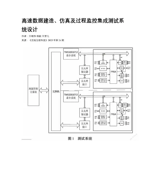
高速数据建造、仿真及过程监控集成测试系统设计作者：王晓伟相毅王梦凡来源：《无线互联科技》2023年第21期摘要：文章提出了一种集数据建造、仿真、过程监控于一体的测试系统架构。

该测试系统不仅具有普通测试设备模拟外设对星载计算机进行一对一功能测试的能力，还能够模拟真实的测试环境产生测试数据以提高产品测试的真实性，并且在系统级测试中监控星载计算机、载荷之间的整个测试过程，快速定位系统级测试中出现的问题。

该测试系统可以有效地解决测试环境不全面以及系统测试中测试过程不透明的问题，提高了产品测试的效率。

关键词：高速；数据建造；仿真；可视化；测试系统中图分类号：TP335 文献标志码：A0 引言随着航空航天领域电子系统信息化和集成度的不断提高，电子产品的交付量也与日俱增，这对产品的测试系统和测试覆盖率提出了更高的要求。

测试系统是每个星载、机载计算机测试必备的设备之一，其主要用来测试产品的功能和性能，确定出产品的运行状态，产品在出现故障时具备故障隔离的能力。

测试系统的好壞往往决定计算机产品能否在真实应用环境中更好地工作，其重要性不言而喻。

测试系统是一种用于检测系统或产品中性能、可用性、功能以及安全性等关键特性的系统。

由于技术进步，实施测试系统变得非常困难，因为它需要复杂而全面的测试计划，其中包括各种测试类型，如功能测试、可用性测试、性能测试等。

目前，所有的测试系统都是通过硬件电路来模拟外设，测试机制比较简单，只是针对性地测试计算机产品各个功能的正确性。

经常存在星载、机载计算机在真实环境中应用时，产品性能不能满足用户的要求以及与载荷联调出现问题时，无法快速进行问题定位，需要消耗大量的人力物力以及时间。

这些问题的根源在于目前的测试系统过于简单，和产品的真实应用环境相差较大，从而导致星载、机载计算机产品的测试覆盖性不全面。

本文针对星载、机载高可靠应用场景，提出了一种集数据建造、仿真、过程监控于一体的测试系统架构。

该测试系统能够模拟计算机产品真实的测试环境产生测试数据以提高产品测试的真实性，并且在系统测试中监控计算机产品和外设之间的整个测试过程，能够快速定位系统级测试中出现的故障。

自动驾驶的伦理和社会问题英语作文Ethical and Social Implications of Autonomous DrivingThe advent of autonomous driving technology has revolutionized the transportation industry, promising a future where cars can navigate without human intervention. This technological advancement has sparked a multitude of discussions surrounding the ethical and social implications of this transformative innovation. As we move closer to a world where self-driving vehicles become a reality, it is crucial to examine the complex issues that arise and consider the impact on individuals, communities, and society as a whole.One of the primary ethical concerns surrounding autonomous driving is the issue of liability and accountability. When a traditional, human-operated vehicle is involved in an accident, the responsibility can be clearly assigned to the driver. However, in the case of autonomous vehicles, the question of who is responsible becomes more complex. Is it the manufacturer of the vehicle, the software developer, the vehicle owner, or the passenger? This ambiguity raises concerns about the potential for legal battles and the need for clear policies and regulations to address liability in the event of an accident.Furthermore, the ethical dilemma of the "trolley problem" becomes particularly relevant in the context of autonomous driving. The trolley problem is a thought experiment that presents a scenario where a runaway trolley is headed towards a group of people, and the only way to save them is to divert the trolley onto a track where it will kill one person instead. In the case of autonomous vehicles, this scenario becomes more complex as the car's onboard systems may need to make split-second decisions that could result in the loss of life. Should the vehicle prioritize the safety of the passengers over pedestrians or vice versa? How should the vehicle's decision-making algorithm be programmed to address such ethical conundrums?Another significant concern is the potential impact of autonomous driving on employment. The transportation industry, particularly the taxi, ride-sharing, and trucking sectors, employs millions of people worldwide. The widespread adoption of autonomous vehicles could lead to the displacement of these workers, raising concerns about job loss and the need for retraining and reskilling programs to help those affected transition to new careers.Additionally, the implementation of autonomous driving technology raises questions about privacy and data security. Self-driving cars are equipped with a vast array of sensors and cameras that collect vast amounts of data about the vehicle's surroundings, the driver'sbehavior, and the passengers' movements. This data could be vulnerable to hacking or misuse, potentially compromising the privacy and security of individuals. Robust data protection policies and cybersecurity measures will be crucial to address these concerns.Furthermore, the deployment of autonomous vehicles may have significant implications for urban planning and infrastructure development. As the transportation landscape evolves, cities will need to adapt their infrastructure to accommodate self-driving cars, including the integration of dedicated lanes, traffic signals, and charging stations. This shift could also impact the design of public spaces, the allocation of parking spaces, and the overall flow of traffic within urban environments.Another important consideration is the potential impact of autonomous driving on social equity and accessibility. While self-driving technology has the potential to provide mobility options for individuals who may have difficulty driving, such as the elderly or those with disabilities, it also raises concerns about the accessibility and affordability of these vehicles, especially for marginalized communities. Ensuring that the benefits of autonomous driving are equitably distributed across all segments of society will be a crucial challenge.Finally, the widespread adoption of autonomous vehicles may havebroader societal implications, such as the impact on public transportation systems, the reduction of traffic congestion, and the environmental consequences of transportation. As self-driving cars become more prevalent, it will be essential to carefully consider these broader societal impacts and develop policies and strategies to address them.In conclusion, the emergence of autonomous driving technology presents a complex array of ethical and social challenges that must be carefully navigated. From issues of liability and accountability to the impact on employment and social equity, the successful integration of self-driving vehicles into our transportation system will require a comprehensive and collaborative approach involving policymakers, industry leaders, and the public. By addressing these concerns proactively, we can work towards a future where the benefits of autonomous driving are realized while mitigating the potential risks and ensuring a more equitable and sustainable transportation landscape.。

腾超小作文Hello, let's embark on a journey through a seamless blend of languages, exploring the beauty of cross-cultural communication. In the realm of technology, innovation has been thriving at an unprecedented pace. The digital revolution has transformed the way we live, work, and interact with the world. From the rise of artificial intelligence to the advancements in blockchain technology, each leap forward opens up new horizons of possibility.在科技领域，创新以前所未有的速度蓬勃发展。

数字革命已经改变了我们生活、工作和与世界互动的方式。

从人工智能的兴起到区块链技术的进步，每一次飞跃都开辟了新的可能性。

The intersection of technology and society is particularly fascinating. As our lives become increasingly interconnected through digital platforms, we are witnessing a merging of physical and virtual worlds. This convergence not only enhances our capabilities but also poses new challenges and ethical considerations.科技与社会的交融尤其令人着迷。

面向基于x86处理器和AMBA 的系统芯片的全系统模拟器PKUsim 86庞九凤,佟 冬,李 皓,何 浪,程 旭(北京大学微处理器研发中心,北京100871)摘 要: 基于周期级全系统模拟器对微体系结构进行系统性能评估成为芯片设计必不可少的环节.虽然x86处理器是当前商业和科学计算领域最广泛采用的处理器,很少有开源的x86模拟器能够满足研究需要.本文面向基于Geode GX x86处理器和AMB A 总线的PKUni ty 86系统芯片,设计并实现了周期级全系统模拟器PKUsim 86.它可以启动Microsoft DOS 、Wi ndows 98、Wi ndows XP 等操作系统,运行典型的x86应用程序.PKUsim 86支持功能模拟和性能模拟的在线切换,其指令模拟速度为0 86MIPS,与真实硬件的对比表明,PKUsim 86具有较高的相对准确度.关键词: 全系统模拟;性能评估;系统芯片;x86处理器中图分类号: TP302 7 文献标识码: A 文章编号: 0372 2112(2011)02 0351 07PKUsim 86:A Cycle Level Fu ll System Simulator forx 86Processor and AMBA Based SoCPANG Jiu feng,TONG Dong,LI Hao,HE Lang,C HE NG Xu(Microprocessor Re se arch and De velopme nt Cente r ,Pe king Unive rsit y ,Be ijing 100871,China)Abstract: Cycle level full system simulator based performance evaluation has been indispensable to increasingly complex System on Chip designs.Although x86processors have been the most ubiquitous processors in both commercial and science comput ing world,there is a scarcity of open source simulators that enable academic researchers to experiment with new x86microprocessor bas ed designs.This paper presents a cycle level full system simulator for PKU nity 86System on Chip platform,which is based on Geode GX x86pro cessor and AM BA bus architecture.PKUsim 86can boot up M icrosoft DO S,Window s 98,Window s XP and ru n common x86applications.On the fly switching between the functional simulation and performance simulation mode is supported.PKUsim 86executes 0 86million simulated instructions per second on pared with real machines,the relative accuracy of PKUsim 86is acceptable.Key words: full system simulation;performance evaluation;system on chip;x86processor1 引言通过对硬件建模,研究者可以用参数可控的形式来考察目标应用程序在被模拟系统上执行时的行为与特征.基于周期精确的性能模拟器对微体系结构进行性能分析和设计空间探索,已经逐渐取代早期数学形式化的性能评价方法[1],成为芯片设计流程的必要环节.现有的大多数模拟器是用户级模拟,比如被广泛应用于超标量处理器微体系结构研究的SimpleScala r 模拟器[2].但是,用户级模拟忽略了中断、系统调用等操作系统代码的执行对系统性能的影响,对SPEC CIN T2000的评测误差可达100%[3].因此,全系统模拟将成为今后体系结构研究和设计的趋势[4].x86处理器是当前商业和科学计算领域使用最广泛的处理器,但目前很少有开源的面向x86处理器的模拟器可用于x86处理器的硬件设计和x86应用程序的研究.从国际的研究现状来看,现有的x86全系统模拟器要么为了保证模拟的详细而降低了实现的灵活性,要么为了灵活性而影响了模拟速度,大都存在修改困难、执行速度慢、对性能模拟的支持有限等问题.仅针对抽象的硬件而非真实的机器建模,无法对模拟器本身存在的误差进行分析和校正,难以获得准确可信的结论.PK Unity 86[5]是一款基于Geode GX x86处理器和AMBA 开放总线架构的系统芯片(System on Chip,SoC),收稿日期:2009 12 03;修回日期:2010 07 26基金项目:国际科技合作基金(No.2008DFB10010)第2期2011年2月电 子 学 报ACTA ELECTRONICA SINICA Vol.39 No.2Feb. 2011支持运行Mic rosoft DOS 、Windo ws 98等操作系统及x86应用程序.其开放的总线架构使得快速集成各种标准I P 核成为可能,充分利用了传统嵌入式领域的设计资源优势,其x86处理器支持运行Microsoft Windows 操作系统及其丰富的x86应用软件,充分利用了传统个人计算机的软件优势.本文设计了面向PK Unity 86系统芯片的周期级全系统模拟器PKUsim 86.P KUsim 86由执行部分、功能模拟和性能模拟等构成,具有以下特征:(1)执行部分与模拟部分分离,具有良好的可重定向性;(2)功能模拟和性能模拟分离,支持在线实时切换,以节省模拟所需的时间;(3)提供灵活的体系结构配置机制;(4)平均每秒模拟执行指令数达到0 86百万条,通过与真实Geode GX x86处理器的校对,保证了模拟器本身的准确度.2 背景介绍2.1 PKUnity 86系统芯片PKUnity 86是基于Ge ode GX x86处理器和AMBA 开放总线架构的SoC [6],其核心功能部件如图1所示.Ge ode GX 处理器是AMD 公司转让给中国的一款32位按序单发射八级流水结构的低功耗x86处理器.CAB(CP U AHB Bridge)负责x86处理器的总线接口协议到AHB 总线协议的转换,以及处理器、存储控制器、主PCI2 2桥之间的通讯.位于32位AHB 总线上的高速系统设备硬盘控制器、静态存储控制器.位于32位APB 总线上的低速外围设备包括串行接口、通用输入输出接口、PS/2接口、复位控制以及传统设备,即可编程中断控制器,可编程中断定时器和实时时钟.AHB 和APB 总线之间通过AHB/APB 桥进行通讯.2.2 相关工作Pin [7]是Intel 公司开发的动态插桩系统(Dyna mic Instrumentation System),将C/C++代码插入正在运行的二进制程序的某些位置,用于探视程序的代码覆盖和执行踪迹、转移预测、Cache 失效率、缺陷容忍、内存泄漏等情况,在分析复杂应用程序行为的研究中有着广泛的应用.动态插桩干扰原始程序的运行,运行速度会降低1/10[8],适用于设计后的硬件机器.Bochs [9]模拟了完整的基于I ntel 80x86处理器的个人计算机系统,可以运行Microsoft D OS 、Windo ws 95/98/N T/2000/XP/2003、GNU/Linux 等操作系统,配置成386、486、Pentium 、Pentium Pro 、Pentium II 、Pentium III 、Pe ntium4和x86 64等处理器.Boc hs 被广泛应用于调试新的操作系统、开发新的设备驱动程序、作为新的x86兼容硬件的参考模型.但是,Bochs 是指令级的全系统模拟器,不支持性能评测.P TLsim [10]模拟x86和x86-64指令系统体系结构(Instruction Set Architecture,ISA)处理器,对高速缓存、存储系统和输入输出设备都进行了性能建模.它通过集成Xe n 虚拟机,直接在宿主机上运行指令,以实现全系统模拟的支持.P TLsim 是目前唯一开放源代码的x86架构周期级全系统模拟器.但是,PTLsim 要求宿主机必须是64位,不支持Microsoft Windo ws 操作系统及x86应用程序,这些局限性使得它不适用于PKUnity 86系统.LLV M (Lo w Level Virtual Mac hine)[11]是美国伊利诺斯大学开发的开放源代码编译器架构.它包括LL VM 虚拟指令集,用于分析、优化、代码生成等工作的集成库,以及建立在以上集成库基础之上的汇编器、链接器和调试器等.PK Usim 86采用GCC 编译器,通过解释执行每一条x86指令,解释执行有很高的兼容性,但速度较慢,基于LLV M 的动态编译器具有很低的兼容性,但是速度却较快.这需要在兼容性和模拟速度之间取得合理的权衡.3 PKUsim 86的设计与实现PK Usim 86的设计目标是修改配置灵活、执行速度快、可重定向.它采用了两种设计原则:执行部分与模拟部分的分离,功能模拟与性能模拟的分离.为了减少非必要的工作量,采用将SESC [12]的x86性能模型融入Bochs 全系统模拟环境中的设计思路.3.1 总体框架与设计原则PK Usim 86由执行部分、功能模拟和性能模拟等三部分组成,如图2所示.执行部分用于控制模拟器的启动、配置和运行,以及与用户的交互.功能模拟由Bochs 和RP T (RePla y Transmogrifie r)[13]完成.性能模拟的核心是SESC.(1)执行部分与模拟部分的分离这是PKUsim 86的首要设计原则.执行部分与模拟部分的关系为松耦合,通过定义交互接口,将执行部分和模拟部分有机地结合起来,使设计者几乎可以完全复用执行部分,只关心目标硬件系统的模拟,易于支持不同目标硬件系统的模拟,从而实现了可重定向性的支持.除x86处理器外,PKUsim 86已经成功移植到Uni Core32处理器和ARM 处理器上.以基于UniCore32处理器的Uni ty 863系统为例说明.通过在模拟部分实现U352 电 子 学 报2011年niCore32处理器、存储系统和输入输出系统的模型,将Bochs替换为UniCore32的指令级功能模拟器sim Uni Core32,并模拟MMU的虚实地址转换行为和实地址空间,由于Unity 863系统的外设与PC基本相同,复用标准的外设模型,并实现Unity 863系统所特有的时钟控制器与中断控制器.(2)功能模拟与性能模拟的分离功能模拟与性能模拟的分离使得在保持一部分不变的情况下另一部分具有更大的灵活性.例如在保证功能模拟不变的情况下,可以支持不同抽象层次的性能模拟,包括交易级、周期级和寄存器传输级等. PKUsim 86中性能模拟的建模粒度是周期级精确.表1是功能模拟与性能模拟的特征.表1 功能模拟与性能模拟的特征项目功能模拟性能模拟输入二进制程序代码微指令序列输出微指令序列性能分析结果模拟任务启动操作系统,运行应用程序执行微指令序列,产生各个部件以及总的详细统计信息抽象层次指令级交易级,周期级,寄存器传输级 该设计原则为功能模拟与性能模拟的在线实时切换提供了支持.性能模拟执行应用程序往往耗费大量的时间,在应用程序进入核心循环或研究人员感兴趣的区域之前,使用功能模拟模式,然后通过用户界面的按钮切换到详细的性能模拟模式,统计性能数据. PKUsim 86为研究者提供了不同模拟粒度的在线切换机制,功能模拟的指令数由研究者决定.在线模拟粒度切换加快系统的启动,从而将有限的时间花费在性能数据的收集.3.2 功能模拟处理器的功能模型是计算机模拟的核心,它模拟了指令级的x86处理器.处理器模型的抽象类接口可以适用于不同的指令系统体系结构,重定向是指从抽象类接口继承并实现目标硬件系统的处理器.图3是处理器模型的类层次.cpu-stub-c是抽象类接口,cpu-c类继承cpu-stub-c类并模拟具体处理器,此处模拟的是x86处理器,其内嵌成员plugin Memsys指向存储系统的抽象接口,cpu-c类具有一个通用的译码方法md-init-dec oder,负责对x86指令进行译码.cpu-loop方法模拟了x86处理器的取指、译码和执行过程,按照图4中的步骤进行无限循环直至退出模拟,具体过程如下:(1)如果发生外部中断,调用handle AsyncEvent方法处理外部中断;(2)取出一条x86指令;(3)对该条x86指令进行译码并执行;(4)更新时钟滴答.系统内部时间的计算是以单条指令的模拟为基本单位的.各个模拟部件均注册自己的时间调度周期和回调函数,在cpu-c类的每个执行步后,通过cpu-loop方法调整事件调度队列中每一项的剩余时钟滴答数,在剩余滴答数减至0时,调用该项注册事件的回调函数.被模拟部件发送中断、检测是否有用户输入等都是通过这种机制来实现的.存储模型是由物理内存和内存管理单元(Memory Management Unit,MMU)组成的.MMU是现代计算机系统中的重要组成部分,负责将虚拟地址转换为物理地址. MMU直接访问内存的页表,当遇到权限受限或Page Fault时,产生异常并将控制转给处理器.另外,MMU还负责维护页表的访问位和脏位,以及分发对内存访问353第 2 期庞九凤:面向基于x86处理器和AMB A的系统芯片的全系统模拟器PKUsim 86和输入输出设备(Input/Output,I/O)的访问.由于是功能模拟,所以没有实现TLB 和Cache,直接访问物理内存来读取和写入数据.PKUsim 86复用了Bochs 中已有的传统个人计算机系统中的输入输出设备模型,包括可编程中断控制器、可编程中断定时器、实时时钟、PS/2接口的键盘和鼠标、主PCI 桥、显卡、IDE 控制器等.RPT 是一个通用的指令译码器,它将特定指令系统体系结构的指令转换为通用的微指令序列.这些微指令序列被性能模型用于详细的模拟.RP T 是微体系结构性能模拟器与ISA 功能参考模型或FPGA 仿真器之间的耦合部件.在PKUsim 86中,RPT 将功能模拟的每条x86指令转换成一组微指令序列,该组微指令序列以指令对象(instruction objec t)的形式提交给性能模型.以x86ISA 中的指令POP %eax 为例,如图5所示,栈中的P OP 指令被转化为两条微指令,第一条微指令uLD 将栈顶的数据写入eax 寄存器中,第二条微指令uSUB 将栈顶指针esp 寄存器的值减4.RP T 将由uLD 和uSUB 组成的一组微指令序列发送给性能模型,由其进行详细的性能模拟评测.POP%eaxuLD%eax,[%esp]uSUB%esp,4图5 x86指令到微指令序列的转换示例3.3 性能模拟处理器的性能模型通过修改SESC 而来.原始的SESC 是一个面向MIPS 指令系统体系结构的性能模拟器,采用MI NT(MI PS 解释器)作为其功能模拟部分.在本文中,我们用Bochs 替换MI NT,从而将SESC 移植到x86指令系统体系结构.SESC 对流水线、分支预测、缓存等进行了详细建模.RP T 将指令对象发给SESC 进行性能模拟,以计算执行所需要的时间.指令对象包含了性能模拟所需的所有信息:指令地址、Load/Store 指令的存储地址、源寄存器、目标寄存器等.图6是SESC 中部分关键类的相互关系.Execution Flow 类控制了SESC 的整个模拟过程,它通过exec ute PC ()和exeInst()方法调用仿真模块执行指令,并产生相应的动态指令类,交由性能模型进行模拟.GProcessor 类模拟了处理器核,控制整个流水线的运行,其取指令功能又通过Fetc hEngine 类实现,FetchEngine 类接收来自RP T 的微指令序列.Resource 类是处理器核中各功能单元的基类,在其之上派生出了定点处理单元、浮点处理单元、分支预测单元、访存处理单元、Cache 和TLB 等类.当GProcessor 类调用issue()方法时,动态指令对象将传递给相应的功能单元进行处理.DepWindo w 类负责检查流水线中正在处理的动态指令对象之间的相关性,决定各条指令是否可发射或进入下一个流水级.Cluster 类则用来协调多处理器的模拟时各功能单元直接的关系.总线的性能模型对AMBA 总线进行了周期级建模,如表2所示,其总线宽度、频率等特性是在总线初始化时指定的.当Cache 或TLB 失效时,处理器的性能模型通过access 方法发起总线请求,并指定总线请求的类型,例如读写类型、地址和控制信息等.总线的性能模型在每个周期都调用bus -loop 方法,该方法进一步调用arbitrate 和dec ode 方法分别对总线请求进行仲裁和译码,并选择相应的从设备进行响应.从设备(此处为内存控制器)通过pluginSla ves 方法注册到总线上,接收并处理总线上的请求.受到预充电、内存刷新、地址译码等影响,内存访问延迟差别很大,而SESC 中原有的内存性能模型指定了固定的内存延迟,难以准确地体现内存对于计算机系统的性能影响.因此,PK Usim 86将DRAMsim [14]集成到性能模型中.DRAMsi m 将处理器发到总线上的访存请求转换成一系列的DRAM 命令序列,并将物理地址进一步地转换成内存的通道ID,体I D,行ID 和列I D 等,用于控制读和写内存数据.由于PK Unity 86SoC 采用DDR2存储控制器,PKUsim 86中的DRAMsim 也被配置成DDR2,以尽可能接近真实的硬件设计.表2 总线的性能模型的特征类型描述i nit 总线初始化,通过参数确定总线的宽度,频率等access 处理器访问总线的调用方法,通过参数确定请求arbi trate 总线仲裁方法,提供总线的仲裁机制decoder 总线地址译码方法,提供地址译码机制bus -loop 总线调用方法,处理每个周期总线的行为pluginSlaves从设备注册方法输入输出设备的行为受外界事件的影响,很难进行精确的性能建模.一般来说,程序中平均只有1%的指令是I/O 指令,大多数设备的I/O 访问很少发生.所以,本文主要关注PKUnity 86SoC 对系统性能有关键影响的部件,包括x86处理器、总线和存储控制器.3.4 其他特性在真实的处理器中,当转移指令预测错误时,错误分支上的指令将进入流水线,直到转移指令的转移方354 电 子 学 报2011年向确定为止.PKUsim 86时序模拟的指令来自于功能模拟,且均被正确执行,为了模拟错误分支上的指令对微体系结构状态的影响,PKUsim 86在流水线中插入若干无关指令,数目由平均转移预测代价决定.模拟器的调试过程将会占据相当大的工作量,必须从设计之初就考虑提供方便的程序调试接口. PKUsim 86提供了两种调试手段:GDB调试插桩和检查点(c heckpoint).P KUsim 86支持利用GDB调试插桩交叉调试被模拟系统,可以对被模拟系统进行源代码级调试.在全系统模拟器中,错误往往发生在程序执行很长时间以后,通过加入检查点的支持,可以在很短时间内恢复到错误现场,从而提高调试的效率.PKUsim 86的另一大特点是通过Perl脚本来控制模拟器的运行并进行性能数据的统计,以及配置文件的修改.由于脚本的解释独立于系统的模拟,脚本的修改无须重新编译模拟器源代码,不会对模拟器的正常运行造成影响.4 实验本文实验的宿主机采用四个2 83GHz Intel Core2 CP U,内存8GB DDR2,硬盘1TB;软件是Fedora Linux,内核版本2 6 24.实验包括模拟器的准确度评测,执行速度评测,以及对设计的指导.4.1 准确度评测PKUnity Hilon开发板上集成了Geode GX x86处理器芯片.通过在P KUsim 86模拟器和PKUnity Hilon开发板的对比实验,评估x86处理器内部的二级TLB (L2TLB)和转移目标缓冲器(BTB)、指令Cache(I Cache)、数据Cac he(DCache)等功能单元对系统性能的影响.本实验采用的基准程序是SPEC CI NT2000.如图7所示,在P KUsim 86模拟器和P KUnity Hilon 开发板上的实验表明,x86处理器内部的功能单元对系统性能的相对影响很接近,例如,关闭L2TLB,PK Usim 86的性能下降为原始被模拟系统的0 950,PKUnity Hilon开发板的性能下降为原始真实硬件机器的0 906.相对于绝对准确度(absolute accurac y)而言,模拟器的相对准确度(relative accuracy)对系统的评测更为关键,研究人员可以基于模拟器对各种不同的设计方案进行对比分析,从而选择较优的设计方案.4.2 模拟速度评测文献[15]指出,典型的指令级功能模拟器每秒平均模拟执行6~7百万条指令(M illion Instruc tion Per Sec ond,MIPS),在真实机器上,平均每秒执行1000~2000百万条指令,功能模拟比本地执行要慢2到3个数量级.对于周期精确的性能模拟而言,模拟速度比功能模拟慢1到2个数量级,平均每秒最多模拟执行0 3百万条指令,比本地执行要慢10,000倍(160h vs.1min).表3列出了P KUsi m 86对不同程序的模拟速度.在PK Usim 86上启动Mic rosoft Windows XP,运行SPEC CI NT2000基准程序子集,以及A TTO Disk,Bench mark1 3f,Crystal Disk Mark,Crystal Mark和Performance Test等评测程序.P KUsim 86每秒模拟执行的周期数最多是4 465百万个周期,最少是2 571百万个周期,平均每秒模拟执行3 569百万个周期.在性能模拟模式下,PK Usim 86的模拟速度最高可达1 136MI PS,最低为0 583MIPS,平均模拟速度为0 86MIPS.表3 PK Us im 86的模拟速度基准程序周期数(K)指令数(K)执行时间(h)MCPS(每秒百万个周期)MIPS(每秒百万条指令) ATTO Dis k1509776793420580511 3.8120.864 Benchmark1.3f1494574533212881 4.1520.923 Crystal DiskMark2255531300147010236 2.5710.583 Performance Tes t1133868929750221 3.1500.879 Crys tal Mark CM09GD I48225169121612784 3.3490.845 Crys tal Mark CM09OG L75549367715731267147 4.4650.930 Crys tal M ark C M09D2D2243881194747693615 4.155 1.136 164.gzip1313945831972901 3.6500.889181.mcf967885524311831 2.6890.675256.bzip2332448510789940925 3.6940.878平均值/// 3.5690.860 PK Usim 86的性能模型采用事件驱动模拟,只在当使某个模块状态改变的事件发生时才去访问该模块,相对于周期驱动模拟而言,节省了计算资源,加快了模拟速度,其模拟速度是一般性能模拟器的2 9倍,远远高于GEMS模拟器[16],GEMS模拟器的指令模拟速度仅为0 12MIPS.4.3 对设计的指导基于PKUsim 86模拟器,我们评估了不同的总线配置对性能的影响,如表4所示.355第 2 期庞九凤:面向基于x86处理器和AMB A的系统芯片的全系统模拟器PKUsim 86表4 不同的总线配置对性能的影响配置总线宽度(位)读操作返回首数据的延迟(CPU 时钟周期数)读操作返回后续数据的延迟(CP U 时钟周期数)平均性能(Instruction Per Cycle,IPC)1324040.2362323030.2793644040.2874643030.313处理器频率为533MHz,DDR2存储控制器频率667MHz,总线频率为266MHz.32位总线只能同时传输1个字(word),当Cac he 失效时,传输第一个字需要m 个CP U 周期,传输后续的每个字需要n 个周期,则完成行填充需要(m +n *(S |LS 1))个周期,其中S |LS 是Cac he 的块大小,而若采用64位总线,行填充仅需要(m +n *(S |LS 1)/2)个周期.提高总线带宽(包括增加总线宽度和提高吞吐率)将有效地提高性能,配置4比配置1的性能提高了32 6%.相对于提高总线吞吐率而言,增加总线宽度更能带来性能的改善,配置2比配置1的性能提高18 2%,而配置3比配置1的性能提高21 6%.通过P KUsi m 86模拟器得到若干关键微体系结构的统计数据,每2百万个周期进行一次采样,图8和图9显示了程序在运行的不同采样点时分支预测错误率,一级数据Cac he 失效率,以及处理器性能的变化,较高的数据Cac he 失效率引起处理器性能的急剧下降,如第133个采样点.正在进行的一项研究是分析x86应用程序中引发一级数据Cache 失效次数最多的重要装载(i mportant load)和关键分支转移(c ritical branch),进而优化load/Store 队列和分支转移预测器的设计,类似的研究参见文献[17,18].5 总结和未来工作本文设计并实现了基于Geode GX x86处理器和AMBA 总线的P KUnity 86系统芯片的周期级全系统模拟器PK Usim 86,启动M icrosoft DOS,Windows98、Windo ws XP 等操作系统和运行典型的x86应用程序.PK Usim 86采用执行部分与模拟部分分离的设计原则,具有较好的可重定向性;支持功能模拟和性能模拟的在线切换,其指令模拟速度可达0 86MIPS,是一般性能模拟器的2 9倍.与真实硬件的对比实验表明,PKUsim 86具有较高的相对准确度.直接执行是在宿主机上执行每条x86指令,其模拟性能还有进一步提升的可能,但直接执行要求目标机器与宿主机具有相同的ISA,这需要在模拟速度与灵活性之间做到合理的权衡.PK Usim 86对多处理器模拟的支持也是正在进行一个重要研究工作.参考文献:[1]林闯,李雅娟,王忠民.性能评价形式化方法的现状和发展[J].电子学报,2002,30(12A):1917-1922.Lin Chuang,L i Ya Ju an,Wang Zhong min.Status and develop ment of formal methods for performance evaluation[J].Acta Electronica Sinica,2002,30(12A):1917-1922.(in Chinese)[2]张福新,章隆兵,胡伟武.基于SimpleScalar 的龙芯CPU 模拟器Sim G odson[J].计算机学报,2007,30(1):68-73.Zhang Fu x i n,Zhang L ong bing ,Hu Wei Wu.Sim Godson:a Godson pro cessor simulator based on SimpleScalar[J].Chinese Journal of Computers,2007,30(1):68-73.(i n Chi nese)[3]Joshua J Y ,Lilja D J.Simulation of computer architectu res:simulators,benchmarks,methodologies and recommendations [J].IEEE T ransaction on Computers,2006,55(3):268-280.[4]赵霞,郭耀,雷志勇,陈向群.基于模拟器的嵌入式操作系统能耗估算与分析[J].电子学报,2008,36(2):209-215.Zhan Xia,G uo Yao,Lei Zhi yong ,Chen Xiang qun.Es timation and analysis of embedded operating system energ y consu mption [J].A cta Electronica Sinica,2008,36(2):209-215.(in Chi nese)[5]Huang Kan,Lu Jun lin,Pang Jiu feng,Zheng Yan song,LiHao ,Tong Dong ,Cheng X u.FPGA prototyping of an AMBAbas ed SoC compatible with M icro s oft Windows[A].Proceed ings of International Symposium on Field Programmable Gate Arrays[C].New Y ork,NY,U SA:ACM ,2010.13-22.[6]郑衍松,佟冬,李皓,庞九凤,程旭.MS Windows 兼容的系统芯片硬件核心的分析与实践[J].北京大学学报(自然科学版),2009,45(6):973-978.Zheng Y an song,Tong Dong,Li Hao,Pang Jiu feng,Cheng Xu.Analysis and practice of a SoC hardware kernel for MS Windows [J ].Acta Scientiarum Naturalium Universitatis Pekinensis,2008,45(6):973-978.(in Chines e)[7]Chi Keung Lul,et al.Pin:building cus tomized program analysistoo ls with dynamic ins trumentation[A ].Proceedings of ACMConference on Programming Language Design and Implementa tion[C].N ew York,NY ,USA :ACM ,2005.190-200.[8]Lizy Kurian John.Performance Evaluation And Benchmarking[M ].Bo ca Raton,FL,U SA:CRC Press,2006.5-25.356电 子 学 报2011年[9]Lawton K,et al.T he Bochs IA 32emulator p ro ject[OL].http://bochs.so u ,2008 06 08/2009 12 03. [10]M att T Y ours t.PTL sim:a cycle accurate full system x86 64micro architectural simulator[A].Proceedings of IEEE Inter national Symposiu m on Performance Analysis of Systems& Software[C].San Jose,CA,USA:IEEE,2007.23-34. [11]Chris Arthur Lattner.LLVM:An Infrastructure for Multi s tageOptimization[D].Urbana,Illi nois:U nivers tiy of Illino is at U r bana Champaign,2002.[12]Ortego P M,Sack P.SESC:SuperESCalar si mulator[OL].http://s o u /projects/sesc/.2004 12 10.[13]Sanjay Patel.ACS Simulator Tools:Replay Transmogrifier[OL]./ACS/tools/,2003/2009.[14]D avid Wang,Brinda Ganesh,et al.DRAM sim:a memory sy stem simulator[J].SIGARCH Computer Architecture New s, 2005,33(4):100-107.[15]A yose F,Paolo F,et bining simulation and virtualization through dynamic sampling[A].Proceedings of IEEE In ternational Sympo sium on Performance Analysis of Systems& Software[C].San Jose,CA,U SA:IEEE,2007.72-83. [16]M ilo M K M arin,et al.M ultifacet s general execution drivenmultiprocessor simulator(GEMS)toolset[J].ACM SIGARCH Computer Architecture News,2005,33(4):92-99.[17]谢学军,叶以正,邱善勤,喻明艳.基于马尔可夫模型的数据值预取方案[J].电子学报,2007,35(2):307-310.Xie X ue jun,Ye Yi zheng,Qiu Shan qin,Y u M ing yan.Datavalue prefetching method based on markov model[J].ActaElectronica Sinica,2007,35(2):307-310.(in Chines e) [18]朱德新,程旭,慎辉.UNICORE体系结构中动态转移预测机制的研究与设计[J].电子学报,2004,32(8):1351-1355.Zhu De xin,Cheng Xu,Shen Hui.Dynamic b ranch predictionresearch and design for UNICORE architecture[J].Acta Electronica Sinica,2004,32(8):1351-1355.(in Chinese)作者简介:庞九凤 女,1985年1月出生于河南濮阳.博士研究生,主要研究领域为软硬件协同设计、计算机模拟和性能评估、系统芯片设计.E mail:pangji ufeng@佟 冬 男,1971年10月生于黑龙江.副教授,主要研究领域为存储系统、片上通信、系统芯片和微处理器系统结构设计、软硬件协同设计.357第 2 期庞九凤:面向基于x86处理器和AMB A的系统芯片的全系统模拟器PKUsim 86。

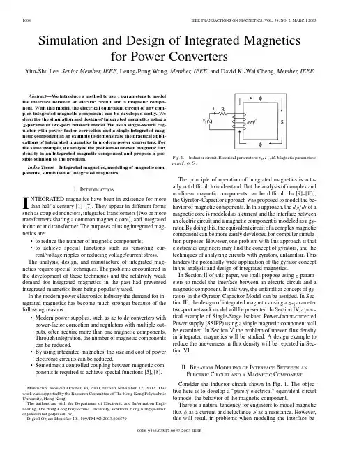
Simulation and Design of Integrated Magneticsfor Power ConvertersYim-Shu Lee,Senior Member,IEEE,Leung-Pong Wong,Member,IEEE,and David Ki-Wai Cheng,Member,IEEEAbstract—We introduce a method touse-parameter two-port network model.We use a single-switch reg-ulator with power-factor-correction and a single integrated mag-netic component as an example to demonstrate the practical appli-cations of integrated magnetics in modern power converters.For the same example,we analyze the problem of uneven magnetic flux density in an integrated magnetic component and propose a pos-sible solution to the problem.Index Terms—Integrated magnetics,modeling of magnetic com-ponents,simulation of integrated magnetics.I.I NTRODUCTIONI NTEGRATED magnetics have been in existence for morethan half a century[1]–[7].They appear in different forms such as coupled inductors,integrated transformers(two or more transformers sharing a common magnetic core),and integrated inductor and transformer.The purposes of using integrated mag-netics are:•to reduce the number of magnetic components;•to achieve special functions such as removing cur-rent/voltage ripples or reducing voltage/current stress. The analysis,design,and manufacture of integrated mag-netics require special techniques.The problems encountered in the development of these techniques and the relatively weak demand for integrated magnetics in the past had prevented integrated magnetics from being popularly used.In the modern power electronics industry the demand for in-tegrated magnetics has become much stronger because of the following reasons.•Modern power supplies,such as ac to dc converters with power-factor correction and regulators with multiple out-puts,often require more than one magnetic components.Through integration,the number of magnetic components can be reduced.•By using integrated magnetics,the size and cost of power electronic circuits can be reduced.•Sometimes a controlled coupling between magnetic com-ponents is required to achieve special functions[5],[8].Manuscript received October30,2000;revised November12,2002.This work was supported by the Research Committee of The Hong Kong Polytechnic University,Hong Kong.The authors are with the Department of Electronic and Information Engi-neering,The Hong Kong Polytechnic University,Kowloon,Hong Kong(e-mail: enyslee@.hk).Digital Object Identifier10.1109/TMAG.2003.808579Fig.1.Inductor circuit.Electrical parameters:v,R.Magnetic parameters: mmf, ,S.The principle of operation of integrated magnetics is actu-ally not difficult to understand.But the analysis of complex and nonlinear magnetic components can be difficult.In[9]–[13], the Gyrator–Capacitor approach was proposed to model the be-havior of magnetic components.In this approach,the of a magnetic core is modeled as a current and the interface between an electric circuit and a magnetic component is modeled as a gy-rator.By doing this,the equivalent circuit of a complex magnetic component can be more easily developed for computer simula-tion purposes.However,one problem with this approach is that electronics engineers may find the concept of gyrators,and the techniques of analyzing circuits with gyrators,unfamiliar.This hinders the potentially wide application of the gyrator concept in the analysis and design of integrated magnetics.In Section II of this paper,we shall proposeusing-parameter two-port network model will be presented.In Section IV,a prac-tical example of Single-Stage Isolated Power-factor-corrected Power supply(SSIPP)using a single magnetic component will be examined.In Section V,the problem of uneven flux density in integrated magnetics will be studied.A design example to reduce the unevenness in flux density will be reported in Sec-tion VI.II.B EHA VIOR M ODELING OF I NTERFACE B ETWEEN ANE LECTRIC C IRCUIT AND A M AGNETIC C OMPONENT Consider the inductor circuit shown in Fig.1.The objec-tive here is to develop a“purely electrical”equivalent circuit to model the behavior of the magnetic component.There is a natural tendency for engineers to model magneticflux as a current andreluctance(a)(b)Fig.2.(a)Electric–magnetic interface.(b)Z -parameter two-port network model of (a).tween the electric circuit and the magnetic component.There-fore,a different approach of modeling is used here.A.Modeling of Electric–Magnetic InterfaceIn this new approach of modeling,we start with the assump-tion that the electric–magnetic interface is to be modeled asa-parameter two-port net-work shown in Fig.2(b),where parameters to be determined.To startwithohms,ohms.Equation (2)truly reflects the induced back electromotive force of the circuit.Theparameter(3)where=N ohms.magnetic short circuit (magnetic material with zero reluctance).The(6)where(9)-parameter two-port network modelof the electric–magnetic interface as shown in Fig.4.It should be noted that although the terminologies of “input port”and “output port”are used,the(a)(b)Fig.5.Modeling of (a)inductor and (b)transformer by equivalent circuit.TABLE IE QUIV ALENCE B ETWEEN M AGNETIC AND E LECTRICAL PARAMETERSone for an inductor as shown in (a),and the other for a trans-former as shown in (b).B.Modeling of Magnetic SaturationWhen the flux density in a nonlinear magnetic core reaches saturation,a large increase in magnetizing force will result in only a small increase in the flux density.Based on the equivalence given in Table I,the magnetic satu-ration phenomenon stated above can be translated into the elec-trical equivalent of:When the charge on a nonlinear capacitor reaches “satura-tion,”a large increase in voltage (across the capacitor)will re-sult in only a small increase in the charge on the capacitor.In [13]and [14],the above-stated phenomenon can be modeled by an equivalent circuit as shown in Fig.6.In this equivalent circuit,the dependent voltagesource(a)(b)Fig.6.(a)Modeling of nonlinear capacitor.(b)Equivalent circuit of nonlinear capacitor.Vn n nnn n nn nn nn n n C.Modeling of Losses in Magnetic ComponentsIn [14]and [15],Eaton proposed adding a core loss resistor tothe Gyrator–Capacitor model to represent the lossy component of a magnetic core.The modified model is referred to as the Gyrator Re-Cap model.When such a lossy component is added tothe––Fig.8.More complete model of transformer.•are used to model the series resistances of thewindings.•are numbers of turns of the primary and sec-ondary windings.III.D ESIGNOF I NTEGRATEDM AGNETICS USING).(a)Possible windingarrangement of an inductorL(a)(b)Fig.10.Integrated inductor (L).(a)Integrated magneticwith two independent (uncoupled)inductors (L(L ).(a)Windingarrangement.(b)Z -parameter two-port network model of (a).Note thatto the center limb of themagnetic core,as shown in Fig.11,inductorand(a)(b)Fig.12.Integrated transformer (T ).(a)Winding arrangement.(b)Z -parameter two-port network model of (a).IV .A PPLICATION E XAMPLEPSpice simulations (based onthe26.9mm,I.D.and a 3C85ETD-39Fig.13.Circuit diagram of Boost–Flyback SSIPP with regenerative clamping.TABLE IIP ARAMETERS OF M AGNETIC C ORES ETD-49AND ETD-39U SED INSSIPPcore is used for thetransformer,a larger magnetic core,3C85ETD-49forboth-param-eter two-port network model ofintegratednF,nF.•nF,nF.•.•are the primary and secondary numbers of turns of the transformer.(The nearest integer numbers closest to the calculated ones are used.The inductance values can be achieved more exactly by adjusting the air gaps.)•are insignificant and ignored in this example.Before putting the circuit to an ac line test,the dc operation was first studied.The input voltage used was 110VDC and the output voltage was regulated at 28VDC.The simulated waveforms of the SSIPP (withseparatedFig.14.Z -parameter two-port network model of integratedLandT=TandT(4A/div);4)i=T (4A/div);4)iFig.19.Experimental waveforms of input line current (1A/div)and line voltage (50V/div)of the SSIPP [with separatedL=TT ini I iL=T=TTh i i i T is icore ETD-39(with an integrated L=T=TFig.27.Simulated waveforms of the SSIPP (with the newL=T(4A/div);4)i=T=T=Ti i i i i i i Th i i i i i i i i i i Th i in i i1018IEEE TRANSACTIONS ON MAGNETICS,VOL.39,NO.2,MARCH2003[7]M.Archer,“Integrated magnetic resonant power converter,”U.S.Patent4774649,Sept.27,1988.[8]P.W.Lee,Y.S.Lee,D.K.W.Cheng,and X.C.Liu,“Steady-stateanalysis of an interleaved boost converter with coupled inductors,”IEEE Trans.Ind.Electron.,vol.47,pp.787–795,Aug.2000.[9] B.D.H.Tellegen,“The gyrator,A new electric network element,”Philips Res.Rep.,vol.3,pp.81–101,Apr.1948.[10]R.W.Buntenbach,“Improved circuit models for inductors wound ondissipative magnetic cores,”in Conf.Rec.2nd Asilomar Conf.Circuits and Systems,Pacific Grove,CA,Oct.1968,pp.229–236.[11],“Analogs between magnetic and electrical circuits,”Electron.Prod.,pp.108–113,Oct.1969.[12] D.C.Hamill,“Lumped equivalent circuits of magnetic components:Thegyrator–capacitor approach,”IEEE Trans.Power Electron.,vol.8,pp.97–103,Apr.1993.[13],“Gyrator–capacitor modeling:A better way of understandingmagnetic components,”in Proc.APEC’94,vol.1,Orlando,FL,Feb.13–17,1994,pp.326–332.[14]M.E.Eaton,“Modeling magnetic devices using the gyrator re-cap coremodel,”in Conf.Rec.,Northcon’94,1994,pp.60–66.[15],“Adding flux paths to SPICE’s analytical capability improves thecase and accuracy of simulating power circuits,”in Proc.APEC’98,vol.1,1998,pp.386–392.[16] D.K.W.Cheng,L.P.Wong,and Y.S.Lee,“Design,modeling,and anal-ysis of integrated magnetics for power converters,”in Proc.PESC’00, vol.1,2000,pp.320–325.[17]Y.S.Lee,K.W.Siu,and B.T.Lin,“Novel single-stage isolatedpower-factor-corrected power supplies with regenerative clamping,”IEEE Trans.Ind.Applicat.,vol.34,pp.1299–1308,Nov./Dec.1998.Yim-Shu Lee(SM’98)received the M.Sc.degree from the University of Southampton,U.K.,in1974,and the Ph.D.degree from the University of Hong Kong in1988.He had been with Cable and Wireless,Rediffusion Television,and the Gen-eral Post Office,all in Hong Kong,before joining The Hong Kong Polytechnic University,Kowloon,in December1969.Currently,he is the Chair Professor of Electronic Engineering in the Department of Electronic and Information En-gineering.He has published more than130technical papers on the design of electronic circuits and is the author of the book Computer-Aided Analysis and Design of Switch-Mode Power Supplies(New York:Marcel Dekker,1993).His current research interests include power electronics and computer-aided design of analog circuits.Dr.Lee is a Fellow of the Institution of Electrical Engineers,U.K.,and the Hong Kong Institution of Engineers.Leung-Pong Wong(S’96–M’98)received the B.Eng.(Hons)degree in electronic engineering in1998from The Hong Kong Polytechnic University, Kowloon,Hong Kong,where he is currently pursuing the Ph.D.degree.His research interests include modeling,simulation,and design of switching power converters,magnetics,and current sensors.David Ki-Wai Cheng(M’90)received the B.Sc.degree with First Class Honor in electronic engineering from Brighton University,U.K.,in1975,and the Ph.D. degree from the University of Hong Kong in1992.He held appointments with Pye Ether Ltd.(U.K.)from1975to1978and Bic-cotest(U.K.)from1978to1983.Currently,he is an Associate Professor with the Department of Electronic and Information Engineering,The Hong Kong Poly-technic University,Kowloon.His research interests include power electronics and computer-aided design of electronic circuits.Dr.Cheng was presented the IEEE Third Millennium Medal in recognition and appreciation of valued services and outstanding contributions.。

International Conference on Advances in Mechanical Engineering and Industrial Informatics (AMEII 2015)Design and Implementation of UAV Flight Simulation Based onMatlab/SimulinkZheng Xing1,a, Yang He2,b, Cheng Jian1,c1Wuhan Mechanical Technology College, Wuhan, 430075, China2Hubei University of Education, Wuhan, 430205, Chinaa email:********************,b email:*****************,c email:**************************omKey words: UAV, Simulation Training, Matlab/Simulink, Flight Simulation, Mode SwitchAbstract.This paper elaborates the composition and function of the flight simulation system according to characteristics of UAV flight simulation in simulation training device. Flight control model and navigation model are designed based on the Matlab/Simulink to solve mode switch and other key technical difficulties in software.IntroductionUA V has been one of important weapon equipment in modern wars and has been widely used in civil areas. As the UA V plays a more and more important role, while accelerating R&D and equipping of advanced UA V system, countries worldwide pay more attention to research of training system and methods based on practical requirements in order to enhance UA V application performance. Currently, extensive developments and applications have been conducted for UA V simulation training systems of different types. The first aim is to improve the ability of flight personnel through simulation training. In order to implement real flight control training, a flight simulation environment should be established[1]. When the effect of flight simulation is closer to real UA V flight status, UA V control personnel’s skills will be improved more.Composition of Flight Simulation SystemFlight simulation computer hardware is composed of an IPC which communicates with system equipment via network port or serial port[2].The software platform is based on general-purpose Windows operating system. In order to simulate the real-time control function of a stabilized turntable, Ardence RTX products will be used. This product offers a real-time subsystem on Windows platform to ensure real-time control, tracking and response on Windows platform. Software consists of two parts: flight control model and navigation model.The former performs digital simulation of real devices of aircraft including aerodynamic device, flight-control computer, actuator, vertical gyro, rate gyro and magnetic heading sensor; the latter controls the UA V to fly at the designated flight path.Design and Implementation of Flight SimulationFor flight control model and navigation model, the mathematical simulation method is used to simulate real devices including flight-control computer, navigation computer, aircraft power and aerodynamic systems and actuator.Development tool.Graphical simulation modeling tool and simulation programming language are mainly used for modeling, and it is Matlab/Simulink that represents a combination of them. The modeling and debugging for the whole flight simulation including aircraft model, control law, sensor model and actuator model are implemented by Matlab/Simulink[3]. Aircraft model and sensormodel can be selected from Simulink model library [4]. For the control law module, S function interfaces written in C/C++ language provided by Simulink can be used to implement mixed programming of Simulink and C/C++ language; then the model can be easily modified and debugged by calling S function written in C/C++ language and making good use of Simulink visual modeling capability.Composition and function. The whole simulation model consists of flight control model (which is used to simulate dynamic characteristics of the aircraft) and navigation model. A six-DoF nonlinear model of aircraft is established based on aerodynamic data. The key to sensor model in the flight control model is how to simulate sensor noise accurately. According to physical properties of the sensor, noise signals are superposed at the output end of the sensor to simulate measured signal noise and error. Dead area, saturation and other nonlinear factors often exist in the actuator. So in the model, dead area and saturation parameters are properly set to simulate the actuator.Flight control model. In a real UA V system, the flight control system is an integrated controller responsible for coordinating and managing all subsystems of the UA V , and is also the core of UA V flight management and control. Therefore, the implementation of the flight control module is a basic and key part in UA V flight simulation.Mathematical modeling. To research into UA V flight control, we first have to establish a model for the research object. In modeling, the following assumptions are always made: the Earth is the inertial reference system; the aircraft is a rigid body; the weight is a constant; and acceleration of gravity does not change with flight altitude. By reference to airframe coordinates, six dynamic differential equations are established to describe the movement of aircraft.[5] The said equations are complex in structure, so they are only suitable for numeric calculation. For the convenience of controller design, a small-disturbance linearized method can be used to obtain the small-disturbance linear state equation of UA V at the equilibrium point.[6] Furthermore, the aircraft is symmetrical, so linear results are divided into two groups, which describe longitudinal movement and lateral movement, respectively. Therefore, five control modes are established for flight control model, including elevation holding and control, altitude holding and control, roll angle holding and control, course angle holding and control, lateral deviation control.The longitudinal small-disturbance linear equation of UA V with wind disturbance is: [7] X AX BU Fd =++where, 100001000010T F = ; 000x y zW V W U d q W x α−∆==∆∆∂∂ ; U 0 is airspeed component along the vertical axis;W x , W y and W z are three components for wind speed; X = [ΔV Δα q Δθ]T ; U = δe .The lateral small-disturbance linear equation of UA V with wind disturbance is: X AX BU Fd =++ where, 100001000010T F= ; 00z y x W U W z d p r W z β∆∂∂==∆∆∂∂ ; U 0 is airspeed component along the vertical axis; W x , W y and W z are three components for wind speed; []T X p βψγ= ; []T a r U δδ=.Design of control law. PID controller is used for the module. The system is under error-based negative feedback control. The controller takes the difference between system output feedback quantity and an expected value or a set value as the input quantity, and with an algorithm, obtains a control quantity to make the output quantity change with the input quantity.[8]Take the design of longitudinal pitch channel of aircraft as an example. The pitch angle and pitch rate feedback are used for pitch attitude holding and control of the aircraft. Pitch rate feedback is realized by the angular rate compensator and the pitch angle is measured by the sensor. The throttle opening is temporarily deemed to be constant, and is not taken into account. Then, the pitch channelcontrol model is designed with Simulink tool kit in Matlab.Navigation model. The navigation system is an integral part of the UA V system. It is capable of providing support for tactical operations of the UA V through satellite navigation, AWACS guiding, ground guiding and UA V capability of detecting and tracking targets. It is mainly used to implement real-time location and automatic control of flight path of the UA V.UA V’s navigation function is based on the coordinated turn function.[9]First, the system determines the current course of an aircraft according to voyage points, measures and calculates the lateral deviation distance between aircraft and flight path, track deviation angle and current ground velocity of aircraft in real time, and then solves a lateral driving signal in accordance with the navigation control law, and gives a bank angle to control the aircraft to enter coordinated turn, and when both lateral deviation distance and track deviation angle are zero, the aircraft performs a straight and level flight along the current flight course until it enters the next point.The simulation of navigation control law is based on flight control law simulation. The navigation control law is designed by integrating each separate channel into full dimension simulation and taking cross track distance and yaw angle as input values.Implementation of Simulation Technology DifficultiesThe flight simulation system is very close to a real system, but different from the real system. In simulation training, UA V is required to perform some extreme actions and random switch among modes, and humanity principle shall be followed during the training. This leads to considerable difficulty and many logical problems in programming. The whole module is of purely digital analog, so mode switch in real-time module may involve problems about zero clearing of many integral terms. In case of failure in timely zero clearing, accumulated values will affect the whole flight simulation result, and even cause systematic divergence, so that the control law could not be successfully implemented. Mutual independence of longitudinal channel and lateral channel is used. When receiving a command about changing longitudinal movement, the system only clears integral terms under longitudinal control, and integral terms under lateral control will keep accumulating until a command about changing lateral movement is received. Zero clearing of lateral integral terms is performed in a similar way.Abovementioned processes will both satisfy requirements of practical simulation training and show simulative extreme action simulation, thereby training operator’s emergency response capability.ConclusionThe flight simulation design of the simulation training device is implemented in the abovementioned method. According to the simulation result, control of modes of the aircraft meets specification requirements, the transition process during switch among modes is stable and the flight profile trend coincides. The design model can truly simulate UA V flight control and navigation and implement real-time simulation of pre-flight preparation, launch, cruising, program-control, manual control, mode switch and recovery controlled by the ground console. It has high confidence level and reliability in simulation, strong expandability and wide application. AcknowledgementThis work is supported by the natural science foundation of Hubei Province No.2014CFB569. This work is also supported by the research project of Hubei Province Department of Education Grant No.Q20133008.References[1] Peng Hua, Shen Weiqun, Song Zishan, A Real-time Management System of Flight SimulationBased on VxWorks, Journal of System Simulation, 2003, 15(7): 966-968.[2] Zhang Ning, Chen Ning, Ji Yun, Zhu Jiang, Research on The Integrated Method of FlightSimulation System Based on A Flight Simulator, Flight Dynamics, 2010, 28(3): 39-42.[3] Zhang Lei, Jiang Hongzhou, Qi Panguo, Li Hongren, Flight Simulation Based on Matlab,Computer Simulation, 2006, 23(6): 57-61.[4] Shang Wenxuan, Wang He, Gao Ya, The Avionic System Platform Based on Flight Simulationof Simulink and Its Application, Electronics Optics & Control, 2014, 21(8): 6-9.[5] Zhang Minglian, Flight Control System, National Defense Industry Press, 1993.[6] Xu Hailiang, Li Junyang, Fei Shumin, Design and Implementation of Digital Flight SimulationPlatform, Journal of Southeast University(Natural Science Edition), 2011, 41(1): 113-117. [7] Su Jijie, Zheng Xing, Lin Dongsheng, Yang Yi, Design and Implementation of SimulativeTraining System for UAV, Journal of System Simulation, 2009, 21(5): 1343-1346.[8] Li Chao, Wang Jiangyun, Han Liang, Development of Fixed Wing Aircraft Flight SimulationSystem Based on Matlab, Journal of System Simulation, 2013, 25(8).[9] Gen Tongfen, Huang Daqing, Full Process Simulation of UAV Auto-pilot Flight Based onSimulink, Aeronautical Computing Technique, 2010, 40(5): 112-116.。

MIPS32™ Architecture For Programmers Volume I: Introduction to the MIPS32™ArchitectureDocument Number: MD00082Revision 2.00June 8, 2003MIPS Technologies, Inc.1225 Charleston RoadMountain View, CA 94043-1353Copyright © 2001-2003 MIPS Technologies Inc. All rights reserved.Copyright ©2001-2003 MIPS Technologies, Inc. All rights reserved.Unpublished rights (if any) reserved under the copyright laws of the United States of America and other countries.This document contains information that is proprietary to MIPS Technologies, Inc. ("MIPS Technologies"). Any copying,reproducing,modifying or use of this information(in whole or in part)that is not expressly permitted in writing by MIPS Technologies or an authorized third party is strictly prohibited. At a minimum, this information is protected under unfair competition and copyright laws. Violations thereof may result in criminal penalties and fines.Any document provided in source format(i.e.,in a modifiable form such as in FrameMaker or Microsoft Word format) is subject to use and distribution restrictions that are independent of and supplemental to any and all confidentiality restrictions. UNDER NO CIRCUMSTANCES MAY A DOCUMENT PROVIDED IN SOURCE FORMAT BE DISTRIBUTED TO A THIRD PARTY IN SOURCE FORMAT WITHOUT THE EXPRESS WRITTEN PERMISSION OF MIPS TECHNOLOGIES, INC.MIPS Technologies reserves the right to change the information contained in this document to improve function,design or otherwise.MIPS Technologies does not assume any liability arising out of the application or use of this information, or of any error or omission in such information. Any warranties, whether express, statutory, implied or otherwise, including but not limited to the implied warranties of merchantability orfitness for a particular purpose,are excluded. Except as expressly provided in any written license agreement from MIPS Technologies or an authorized third party,the furnishing of this document does not give recipient any license to any intellectual property rights,including any patent rights, that cover the information in this document.The information contained in this document shall not be exported or transferred for the purpose of reexporting in violation of any U.S. or non-U.S. regulation, treaty, Executive Order, law, statute, amendment or supplement thereto. The information contained in this document constitutes one or more of the following: commercial computer software, commercial computer software documentation or other commercial items.If the user of this information,or any related documentation of any kind,including related technical data or manuals,is an agency,department,or other entity of the United States government ("Government"), the use, duplication, reproduction, release, modification, disclosure, or transfer of this information, or any related documentation of any kind, is restricted in accordance with Federal Acquisition Regulation12.212for civilian agencies and Defense Federal Acquisition Regulation Supplement227.7202 for military agencies.The use of this information by the Government is further restricted in accordance with the terms of the license agreement(s) and/or applicable contract terms and conditions covering this information from MIPS Technologies or an authorized third party.MIPS,R3000,R4000,R5000and R10000are among the registered trademarks of MIPS Technologies,Inc.in the United States and other countries,and MIPS16,MIPS16e,MIPS32,MIPS64,MIPS-3D,MIPS-based,MIPS I,MIPS II,MIPS III,MIPS IV,MIPS V,MIPSsim,SmartMIPS,MIPS Technologies logo,4K,4Kc,4Km,4Kp,4KE,4KEc,4KEm,4KEp, 4KS, 4KSc, 4KSd, M4K, 5K, 5Kc, 5Kf, 20Kc, 25Kf, ASMACRO, ATLAS, At the Core of the User Experience., BusBridge, CoreFPGA, CoreLV, EC, JALGO, MALTA, MDMX, MGB, PDtrace, Pipeline, Pro, Pro Series, SEAD, SEAD-2, SOC-it and YAMON are among the trademarks of MIPS Technologies, Inc.All other trademarks referred to herein are the property of their respective owners.Template: B1.08, Built with tags: 2B ARCH MIPS32MIPS32™ Architecture For Programmers Volume I, Revision 2.00 Copyright © 2001-2003 MIPS Technologies Inc. All rights reserved.Table of ContentsChapter 1 About This Book (1)1.1 Typographical Conventions (1)1.1.1 Italic Text (1)1.1.2 Bold Text (1)1.1.3 Courier Text (1)1.2 UNPREDICTABLE and UNDEFINED (2)1.2.1 UNPREDICTABLE (2)1.2.2 UNDEFINED (2)1.3 Special Symbols in Pseudocode Notation (2)1.4 For More Information (4)Chapter 2 The MIPS Architecture: An Introduction (7)2.1 MIPS32 and MIPS64 Overview (7)2.1.1 Historical Perspective (7)2.1.2 Architectural Evolution (7)2.1.3 Architectural Changes Relative to the MIPS I through MIPS V Architectures (9)2.2 Compliance and Subsetting (9)2.3 Components of the MIPS Architecture (10)2.3.1 MIPS Instruction Set Architecture (ISA) (10)2.3.2 MIPS Privileged Resource Architecture (PRA) (10)2.3.3 MIPS Application Specific Extensions (ASEs) (10)2.3.4 MIPS User Defined Instructions (UDIs) (11)2.4 Architecture Versus Implementation (11)2.5 Relationship between the MIPS32 and MIPS64 Architectures (11)2.6 Instructions, Sorted by ISA (12)2.6.1 List of MIPS32 Instructions (12)2.6.2 List of MIPS64 Instructions (13)2.7 Pipeline Architecture (13)2.7.1 Pipeline Stages and Execution Rates (13)2.7.2 Parallel Pipeline (14)2.7.3 Superpipeline (14)2.7.4 Superscalar Pipeline (14)2.8 Load/Store Architecture (15)2.9 Programming Model (15)2.9.1 CPU Data Formats (16)2.9.2 FPU Data Formats (16)2.9.3 Coprocessors (CP0-CP3) (16)2.9.4 CPU Registers (16)2.9.5 FPU Registers (18)2.9.6 Byte Ordering and Endianness (21)2.9.7 Memory Access Types (25)2.9.8 Implementation-Specific Access Types (26)2.9.9 Cache Coherence Algorithms and Access Types (26)2.9.10 Mixing Access Types (26)Chapter 3 Application Specific Extensions (27)3.1 Description of ASEs (27)3.2 List of Application Specific Instructions (28)3.2.1 The MIPS16e Application Specific Extension to the MIPS32Architecture (28)3.2.2 The MDMX Application Specific Extension to the MIPS64 Architecture (28)3.2.3 The MIPS-3D Application Specific Extension to the MIPS64 Architecture (28)MIPS32™ Architecture For Programmers Volume I, Revision 2.00i Copyright © 2001-2003 MIPS Technologies Inc. All rights reserved.3.2.4 The SmartMIPS Application Specific Extension to the MIPS32 Architecture (28)Chapter 4 Overview of the CPU Instruction Set (29)4.1 CPU Instructions, Grouped By Function (29)4.1.1 CPU Load and Store Instructions (29)4.1.2 Computational Instructions (32)4.1.3 Jump and Branch Instructions (35)4.1.4 Miscellaneous Instructions (37)4.1.5 Coprocessor Instructions (40)4.2 CPU Instruction Formats (41)Chapter 5 Overview of the FPU Instruction Set (43)5.1 Binary Compatibility (43)5.2 Enabling the Floating Point Coprocessor (44)5.3 IEEE Standard 754 (44)5.4 FPU Data Types (44)5.4.1 Floating Point Formats (44)5.4.2 Fixed Point Formats (48)5.5 Floating Point Register Types (48)5.5.1 FPU Register Models (49)5.5.2 Binary Data Transfers (32-Bit and 64-Bit) (49)5.5.3 FPRs and Formatted Operand Layout (50)5.6 Floating Point Control Registers (FCRs) (50)5.6.1 Floating Point Implementation Register (FIR, CP1 Control Register 0) (51)5.6.2 Floating Point Control and Status Register (FCSR, CP1 Control Register 31) (53)5.6.3 Floating Point Condition Codes Register (FCCR, CP1 Control Register 25) (55)5.6.4 Floating Point Exceptions Register (FEXR, CP1 Control Register 26) (56)5.6.5 Floating Point Enables Register (FENR, CP1 Control Register 28) (56)5.7 Formats of Values Used in FP Registers (57)5.8 FPU Exceptions (58)5.8.1 Exception Conditions (59)5.9 FPU Instructions (62)5.9.1 Data Transfer Instructions (62)5.9.2 Arithmetic Instructions (63)5.9.3 Conversion Instructions (65)5.9.4 Formatted Operand-Value Move Instructions (66)5.9.5 Conditional Branch Instructions (67)5.9.6 Miscellaneous Instructions (68)5.10 Valid Operands for FPU Instructions (68)5.11 FPU Instruction Formats (70)5.11.1 Implementation Note (71)Appendix A Instruction Bit Encodings (75)A.1 Instruction Encodings and Instruction Classes (75)A.2 Instruction Bit Encoding Tables (75)A.3 Floating Point Unit Instruction Format Encodings (82)Appendix B Revision History (85)ii MIPS32™ Architecture For Programmers Volume I, Revision 2.00 Copyright © 2001-2003 MIPS Technologies Inc. All rights reserved.Figure 2-1: Relationship between the MIPS32 and MIPS64 Architectures (11)Figure 2-2: One-Deep Single-Completion Instruction Pipeline (13)Figure 2-3: Four-Deep Single-Completion Pipeline (14)Figure 2-4: Four-Deep Superpipeline (14)Figure 2-5: Four-Way Superscalar Pipeline (15)Figure 2-6: CPU Registers (18)Figure 2-7: FPU Registers for a 32-bit FPU (20)Figure 2-8: FPU Registers for a 64-bit FPU if Status FR is 1 (21)Figure 2-9: FPU Registers for a 64-bit FPU if Status FR is 0 (22)Figure 2-10: Big-Endian Byte Ordering (23)Figure 2-11: Little-Endian Byte Ordering (23)Figure 2-12: Big-Endian Data in Doubleword Format (24)Figure 2-13: Little-Endian Data in Doubleword Format (24)Figure 2-14: Big-Endian Misaligned Word Addressing (25)Figure 2-15: Little-Endian Misaligned Word Addressing (25)Figure 3-1: MIPS ISAs and ASEs (27)Figure 3-2: User-Mode MIPS ISAs and Optional ASEs (27)Figure 4-1: Immediate (I-Type) CPU Instruction Format (42)Figure 4-2: Jump (J-Type) CPU Instruction Format (42)Figure 4-3: Register (R-Type) CPU Instruction Format (42)Figure 5-1: Single-Precisions Floating Point Format (S) (45)Figure 5-2: Double-Precisions Floating Point Format (D) (45)Figure 5-3: Paired Single Floating Point Format (PS) (46)Figure 5-4: Word Fixed Point Format (W) (48)Figure 5-5: Longword Fixed Point Format (L) (48)Figure 5-6: FPU Word Load and Move-to Operations (49)Figure 5-7: FPU Doubleword Load and Move-to Operations (50)Figure 5-8: Single Floating Point or Word Fixed Point Operand in an FPR (50)Figure 5-9: Double Floating Point or Longword Fixed Point Operand in an FPR (50)Figure 5-10: Paired-Single Floating Point Operand in an FPR (50)Figure 5-11: FIR Register Format (51)Figure 5-12: FCSR Register Format (53)Figure 5-13: FCCR Register Format (55)Figure 5-14: FEXR Register Format (56)Figure 5-15: FENR Register Format (56)Figure 5-16: Effect of FPU Operations on the Format of Values Held in FPRs (58)Figure 5-17: I-Type (Immediate) FPU Instruction Format (71)Figure 5-18: R-Type (Register) FPU Instruction Format (71)Figure 5-19: Register-Immediate FPU Instruction Format (71)Figure 5-20: Condition Code, Immediate FPU Instruction Format (71)Figure 5-21: Formatted FPU Compare Instruction Format (71)Figure 5-22: FP RegisterMove, Conditional Instruction Format (71)Figure 5-23: Four-Register Formatted Arithmetic FPU Instruction Format (72)Figure 5-24: Register Index FPU Instruction Format (72)Figure 5-25: Register Index Hint FPU Instruction Format (72)Figure 5-26: Condition Code, Register Integer FPU Instruction Format (72)Figure A-1: Sample Bit Encoding Table (76)MIPS32™ Architecture For Programmers Volume I, Revision 2.00iii Copyright © 2001-2003 MIPS Technologies Inc. All rights reserved.Table 1-1: Symbols Used in Instruction Operation Statements (2)Table 2-1: MIPS32 Instructions (12)Table 2-2: MIPS64 Instructions (13)Table 2-3: Unaligned Load and Store Instructions (24)Table 4-1: Load and Store Operations Using Register + Offset Addressing Mode (30)Table 4-2: Aligned CPU Load/Store Instructions (30)Table 4-3: Unaligned CPU Load and Store Instructions (31)Table 4-4: Atomic Update CPU Load and Store Instructions (31)Table 4-5: Coprocessor Load and Store Instructions (31)Table 4-6: FPU Load and Store Instructions Using Register+Register Addressing (32)Table 4-7: ALU Instructions With an Immediate Operand (33)Table 4-8: Three-Operand ALU Instructions (33)Table 4-9: Two-Operand ALU Instructions (34)Table 4-10: Shift Instructions (34)Table 4-11: Multiply/Divide Instructions (35)Table 4-12: Unconditional Jump Within a 256 Megabyte Region (36)Table 4-13: PC-Relative Conditional Branch Instructions Comparing Two Registers (36)Table 4-14: PC-Relative Conditional Branch Instructions Comparing With Zero (37)Table 4-15: Deprecated Branch Likely Instructions (37)Table 4-16: Serialization Instruction (38)Table 4-17: System Call and Breakpoint Instructions (38)Table 4-18: Trap-on-Condition Instructions Comparing Two Registers (38)Table 4-19: Trap-on-Condition Instructions Comparing an Immediate Value (38)Table 4-20: CPU Conditional Move Instructions (39)Table 4-21: Prefetch Instructions (39)Table 4-22: NOP Instructions (40)Table 4-23: Coprocessor Definition and Use in the MIPS Architecture (40)Table 4-24: CPU Instruction Format Fields (42)Table 5-1: Parameters of Floating Point Data Types (45)Table 5-2: Value of Single or Double Floating Point DataType Encoding (46)Table 5-3: Value Supplied When a New Quiet NaN Is Created (47)Table 5-4: FIR Register Field Descriptions (51)Table 5-5: FCSR Register Field Descriptions (53)Table 5-6: Cause, Enable, and Flag Bit Definitions (55)Table 5-7: Rounding Mode Definitions (55)Table 5-8: FCCR Register Field Descriptions (56)Table 5-9: FEXR Register Field Descriptions (56)Table 5-10: FENR Register Field Descriptions (57)Table 5-11: Default Result for IEEE Exceptions Not Trapped Precisely (60)Table 5-12: FPU Data Transfer Instructions (62)Table 5-13: FPU Loads and Stores Using Register+Offset Address Mode (63)Table 5-14: FPU Loads and Using Register+Register Address Mode (63)Table 5-15: FPU Move To and From Instructions (63)Table 5-16: FPU IEEE Arithmetic Operations (64)Table 5-17: FPU-Approximate Arithmetic Operations (64)Table 5-18: FPU Multiply-Accumulate Arithmetic Operations (65)Table 5-19: FPU Conversion Operations Using the FCSR Rounding Mode (65)Table 5-20: FPU Conversion Operations Using a Directed Rounding Mode (65)Table 5-21: FPU Formatted Operand Move Instructions (66)Table 5-22: FPU Conditional Move on True/False Instructions (66)iv MIPS32™ Architecture For Programmers Volume I, Revision 2.00 Copyright © 2001-2003 MIPS Technologies Inc. All rights reserved.Table 5-23: FPU Conditional Move on Zero/Nonzero Instructions (67)Table 5-24: FPU Conditional Branch Instructions (67)Table 5-25: Deprecated FPU Conditional Branch Likely Instructions (67)Table 5-26: CPU Conditional Move on FPU True/False Instructions (68)Table 5-27: FPU Operand Format Field (fmt, fmt3) Encoding (68)Table 5-28: Valid Formats for FPU Operations (69)Table 5-29: FPU Instruction Format Fields (72)Table A-1: Symbols Used in the Instruction Encoding Tables (76)Table A-2: MIPS32 Encoding of the Opcode Field (77)Table A-3: MIPS32 SPECIAL Opcode Encoding of Function Field (78)Table A-4: MIPS32 REGIMM Encoding of rt Field (78)Table A-5: MIPS32 SPECIAL2 Encoding of Function Field (78)Table A-6: MIPS32 SPECIAL3 Encoding of Function Field for Release 2 of the Architecture (78)Table A-7: MIPS32 MOVCI Encoding of tf Bit (79)Table A-8: MIPS32 SRL Encoding of Shift/Rotate (79)Table A-9: MIPS32 SRLV Encoding of Shift/Rotate (79)Table A-10: MIPS32 BSHFL Encoding of sa Field (79)Table A-11: MIPS32 COP0 Encoding of rs Field (79)Table A-12: MIPS32 COP0 Encoding of Function Field When rs=CO (80)Table A-13: MIPS32 COP1 Encoding of rs Field (80)Table A-14: MIPS32 COP1 Encoding of Function Field When rs=S (80)Table A-15: MIPS32 COP1 Encoding of Function Field When rs=D (81)Table A-16: MIPS32 COP1 Encoding of Function Field When rs=W or L (81)Table A-17: MIPS64 COP1 Encoding of Function Field When rs=PS (81)Table A-18: MIPS32 COP1 Encoding of tf Bit When rs=S, D, or PS, Function=MOVCF (81)Table A-19: MIPS32 COP2 Encoding of rs Field (82)Table A-20: MIPS64 COP1X Encoding of Function Field (82)Table A-21: Floating Point Unit Instruction Format Encodings (82)MIPS32™ Architecture For Programmers Volume I, Revision 2.00v Copyright © 2001-2003 MIPS Technologies Inc. All rights reserved.vi MIPS32™ Architecture For Programmers Volume I, Revision 2.00 Copyright © 2001-2003 MIPS Technologies Inc. All rights reserved.Chapter 1About This BookThe MIPS32™ Architecture For Programmers V olume I comes as a multi-volume set.•V olume I describes conventions used throughout the document set, and provides an introduction to the MIPS32™Architecture•V olume II provides detailed descriptions of each instruction in the MIPS32™ instruction set•V olume III describes the MIPS32™Privileged Resource Architecture which defines and governs the behavior of the privileged resources included in a MIPS32™ processor implementation•V olume IV-a describes the MIPS16e™ Application-Specific Extension to the MIPS32™ Architecture•V olume IV-b describes the MDMX™ Application-Specific Extension to the MIPS32™ Architecture and is notapplicable to the MIPS32™ document set•V olume IV-c describes the MIPS-3D™ Application-Specific Extension to the MIPS64™ Architecture and is notapplicable to the MIPS32™ document set•V olume IV-d describes the SmartMIPS™Application-Specific Extension to the MIPS32™ Architecture1.1Typographical ConventionsThis section describes the use of italic,bold and courier fonts in this book.1.1.1Italic Text•is used for emphasis•is used for bits,fields,registers, that are important from a software perspective (for instance, address bits used bysoftware,and programmablefields and registers),and variousfloating point instruction formats,such as S,D,and PS •is used for the memory access types, such as cached and uncached1.1.2Bold Text•represents a term that is being defined•is used for bits andfields that are important from a hardware perspective (for instance,register bits, which are not programmable but accessible only to hardware)•is used for ranges of numbers; the range is indicated by an ellipsis. For instance,5..1indicates numbers 5 through 1•is used to emphasize UNPREDICTABLE and UNDEFINED behavior, as defined below.1.1.3Courier TextCourier fixed-width font is used for text that is displayed on the screen, and for examples of code and instruction pseudocode.MIPS32™ Architecture For Programmers Volume I, Revision 2.001 Copyright © 2001-2003 MIPS Technologies Inc. All rights reserved.Chapter 1 About This Book1.2UNPREDICTABLE and UNDEFINEDThe terms UNPREDICTABLE and UNDEFINED are used throughout this book to describe the behavior of theprocessor in certain cases.UNDEFINED behavior or operations can occur only as the result of executing instructions in a privileged mode (i.e., in Kernel Mode or Debug Mode, or with the CP0 usable bit set in the Status register).Unprivileged software can never cause UNDEFINED behavior or operations. Conversely, both privileged andunprivileged software can cause UNPREDICTABLE results or operations.1.2.1UNPREDICTABLEUNPREDICTABLE results may vary from processor implementation to implementation,instruction to instruction,or as a function of time on the same implementation or instruction. Software can never depend on results that areUNPREDICTABLE.UNPREDICTABLE operations may cause a result to be generated or not.If a result is generated, it is UNPREDICTABLE.UNPREDICTABLE operations may cause arbitrary exceptions.UNPREDICTABLE results or operations have several implementation restrictions:•Implementations of operations generating UNPREDICTABLE results must not depend on any data source(memory or internal state) which is inaccessible in the current processor mode•UNPREDICTABLE operations must not read, write, or modify the contents of memory or internal state which is inaccessible in the current processor mode. For example,UNPREDICTABLE operations executed in user modemust not access memory or internal state that is only accessible in Kernel Mode or Debug Mode or in another process •UNPREDICTABLE operations must not halt or hang the processor1.2.2UNDEFINEDUNDEFINED operations or behavior may vary from processor implementation to implementation, instruction toinstruction, or as a function of time on the same implementation or instruction.UNDEFINED operations or behavior may vary from nothing to creating an environment in which execution can no longer continue.UNDEFINED operations or behavior may cause data loss.UNDEFINED operations or behavior has one implementation restriction:•UNDEFINED operations or behavior must not cause the processor to hang(that is,enter a state from which there is no exit other than powering down the processor).The assertion of any of the reset signals must restore the processor to an operational state1.3Special Symbols in Pseudocode NotationIn this book, algorithmic descriptions of an operation are described as pseudocode in a high-level language notation resembling Pascal. Special symbols used in the pseudocode notation are listed in Table 1-1.Table 1-1 Symbols Used in Instruction Operation StatementsSymbol Meaning←Assignment=, ≠Tests for equality and inequality||Bit string concatenationx y A y-bit string formed by y copies of the single-bit value x2MIPS32™ Architecture For Programmers Volume I, Revision 2.00 Copyright © 2001-2003 MIPS Technologies Inc. All rights reserved.1.3Special Symbols in Pseudocode Notationb#n A constant value n in base b.For instance10#100represents the decimal value100,2#100represents the binary value 100 (decimal 4), and 16#100 represents the hexadecimal value 100 (decimal 256). If the "b#" prefix is omitted, the default base is 10.x y..z Selection of bits y through z of bit string x.Little-endian bit notation(rightmost bit is0)is used.If y is less than z, this expression is an empty (zero length) bit string.+, −2’s complement or floating point arithmetic: addition, subtraction∗, ×2’s complement or floating point multiplication (both used for either)div2’s complement integer divisionmod2’s complement modulo/Floating point division<2’s complement less-than comparison>2’s complement greater-than comparison≤2’s complement less-than or equal comparison≥2’s complement greater-than or equal comparisonnor Bitwise logical NORxor Bitwise logical XORand Bitwise logical ANDor Bitwise logical ORGPRLEN The length in bits (32 or 64) of the CPU general-purpose registersGPR[x]CPU general-purpose register x. The content of GPR[0] is always zero.SGPR[s,x]In Release 2 of the Architecture, multiple copies of the CPU general-purpose registers may be implemented.SGPR[s,x] refers to GPR set s, register x. GPR[x] is a short-hand notation for SGPR[ SRSCtl CSS, x].FPR[x]Floating Point operand register xFCC[CC]Floating Point condition code CC.FCC[0] has the same value as COC[1].FPR[x]Floating Point (Coprocessor unit 1), general register xCPR[z,x,s]Coprocessor unit z, general register x,select sCP2CPR[x]Coprocessor unit 2, general register xCCR[z,x]Coprocessor unit z, control register xCP2CCR[x]Coprocessor unit 2, control register xCOC[z]Coprocessor unit z condition signalXlat[x]Translation of the MIPS16e GPR number x into the corresponding 32-bit GPR numberBigEndianMem Endian mode as configured at chip reset (0→Little-Endian, 1→ Big-Endian). Specifies the endianness of the memory interface(see LoadMemory and StoreMemory pseudocode function descriptions),and the endianness of Kernel and Supervisor mode execution.BigEndianCPU The endianness for load and store instructions (0→ Little-Endian, 1→ Big-Endian). In User mode, this endianness may be switched by setting the RE bit in the Status register.Thus,BigEndianCPU may be computed as (BigEndianMem XOR ReverseEndian).Table 1-1 Symbols Used in Instruction Operation StatementsSymbol MeaningChapter 1 About This Book1.4For More InformationVarious MIPS RISC processor manuals and additional information about MIPS products can be found at the MIPS URL:ReverseEndianSignal to reverse the endianness of load and store instructions.This feature is available in User mode only,and is implemented by setting the RE bit of the Status register.Thus,ReverseEndian may be computed as (SR RE and User mode).LLbitBit of virtual state used to specify operation for instructions that provide atomic read-modify-write.LLbit is set when a linked load occurs; it is tested and cleared by the conditional store. It is cleared, during other CPU operation,when a store to the location would no longer be atomic.In particular,it is cleared by exception return instructions.I :,I+n :,I-n :This occurs as a prefix to Operation description lines and functions as a label. It indicates the instruction time during which the pseudocode appears to “execute.” Unless otherwise indicated, all effects of the currentinstruction appear to occur during the instruction time of the current instruction.No label is equivalent to a time label of I . Sometimes effects of an instruction appear to occur either earlier or later — that is, during theinstruction time of another instruction.When this happens,the instruction operation is written in sections labeled with the instruction time,relative to the current instruction I ,in which the effect of that pseudocode appears to occur.For example,an instruction may have a result that is not available until after the next instruction.Such an instruction has the portion of the instruction operation description that writes the result register in a section labeled I +1.The effect of pseudocode statements for the current instruction labelled I +1appears to occur “at the same time”as the effect of pseudocode statements labeled I for the following instruction.Within one pseudocode sequence,the effects of the statements take place in order. However, between sequences of statements for differentinstructions that occur “at the same time,” there is no defined order. Programs must not depend on a particular order of evaluation between such sections.PCThe Program Counter value.During the instruction time of an instruction,this is the address of the instruction word. The address of the instruction that occurs during the next instruction time is determined by assigning a value to PC during an instruction time. If no value is assigned to PC during an instruction time by anypseudocode statement,it is automatically incremented by either 2(in the case of a 16-bit MIPS16e instruction)or 4before the next instruction time.A taken branch assigns the target address to the PC during the instruction time of the instruction in the branch delay slot.PABITSThe number of physical address bits implemented is represented by the symbol PABITS.As such,if 36physical address bits were implemented, the size of the physical address space would be 2PABITS = 236 bytes.FP32RegistersModeIndicates whether the FPU has 32-bit or 64-bit floating point registers (FPRs).In MIPS32,the FPU has 3232-bit FPRs in which 64-bit data types are stored in even-odd pairs of FPRs.In MIPS64,the FPU has 3264-bit FPRs in which 64-bit data types are stored in any FPR.In MIPS32implementations,FP32RegistersMode is always a 0.MIPS64implementations have a compatibility mode in which the processor references the FPRs as if it were a MIPS32 implementation. In such a caseFP32RegisterMode is computed from the FR bit in the Status register.If this bit is a 0,the processor operates as if it had 32 32-bit FPRs. If this bit is a 1, the processor operates with 32 64-bit FPRs.The value of FP32RegistersMode is computed from the FR bit in the Status register.InstructionInBranchDelaySlotIndicates whether the instruction at the Program Counter address was executed in the delay slot of a branch or jump. This condition reflects the dynamic state of the instruction, not the static state. That is, the value is false if a branch or jump occurs to an instruction whose PC immediately follows a branch or jump, but which is not executed in the delay slot of a branch or jump.SignalException(exce ption, argument)Causes an exception to be signaled, using the exception parameter as the type of exception and the argument parameter as an exception-specific argument). Control does not return from this pseudocode function - the exception is signaled at the point of the call.Table 1-1 Symbols Used in Instruction Operation StatementsSymbolMeaning。

simulation 形容词simulation (形容词) - simulated or imitated closely according to models or patterns1. The flight simulator provided a realistic simulation of flying a fighter jet.飞行模拟器提供了逼真的战斗机飞行模拟体验。

2. The business simulation game allowed participants to experience running a virtual company.这个商业模拟游戏让参与者能够体验经营一个虚拟公司。

3. The virtual reality headset created a simulation of being underwater.这款虚拟现实头盔创造了一种水下的模拟体验。

4. The flight attendant training included a simulation of emergency situations.乘务员培训包括紧急情况的模拟。

5. The simulation exercise helped doctors practice performing surgeries before operating on real patients.模拟训练有助于医生在进行实际手术之前进行实践。

6. The video game provided a simulation of being a professional athlete on the soccer field.这个电子游戏提供了一个模拟身份成为职业足球运动员的体验。

7. The military used a simulation of a battlefield to train soldiers for combat scenarios.军方使用战场模拟训练士兵应对战斗场景。

计算机常用名词的英文缩写GUI:图形用户界面(Graphics User interface)SQL:结构化查询语言(Structured Query Language) &&用于数据库的操作.DDL:数据定义语言(Data Definition Language)DML:数据处理语言(Data Manipulation Language)DLL:动态链接库(Dynamic link library)DIY:自己动手(Do it yourself)COP:流控制语句(Control-of-flow) &&SQLserver数据库中使用.DTE:数据终端设备(Data Terminal Equipment)DCE:数据电路终接设备(Data circuit-teminating equipment)OLE:对象连接与嵌入(Object link and embed)PAD:装配拆卸设备(Packet assembler disassemble)NCC:网络控制中心(Network control center)IMP:接口信息处理机(Interface message processor)PSE:分组交换设备(Packet switching exchanger)SCS:综合布线系统(Structure cabling system)GSM:数字通信&&传统上说的'大哥大'RAM:随机存储器=>'内存'(Random Access Memory)ROM:只读存储器(Read－Only Memory)EDO:扩充数据输出(Extended Data Output)SDRAM:同步动态随机存储器=>同步DRAM (Synchronous Dynamic Random Access Memory)Cache高速缓冲存储器,是位于CPU和主存储器DRAM(Dynamic Randon Access Memory)之间，规模较小，但速度很高的存储器，通常由SRAM(Static Random Access Memory静态存储器)组成。