M. Algorithms for openings of binary and label images with rectangular structuring elements

算法导论第三版第⼆章第⼀节习题答案2.1-1：以图2-2为模型，说明INSERTION-SORT在数组A=<31,41,59,26,41,58>上的执⾏过程。

NewImage2.1-2：重写过程INSERTION-SORT，使之按⾮升序（⽽不是按⾮降序）排序。

注意，跟之前升序的写法只有⼀个地⽅不⼀样：NewImage2.1-3：考虑下⾯的查找问题：输⼊：⼀列数A=<a1,a2,…,an >和⼀个值v输出：下标i，使得v=A[i]，或者当v不在A中出现时为NIL。

写出针对这个问题的现⾏查找的伪代码，它顺序地扫描整个序列以查找v。

利⽤循环不变式证明算法的正确性。

确保所给出的循环不变式满⾜三个必要的性质。

（2.1-3 Consider the searching problem:Input: A sequence of n numbers A D ha1; a2; : : : ;ani and a value _.Output: An index i such that _ D AOEi_ or the special value NIL if _ does not appear in A.Write pseudocode for linear search, which scans through the sequence, looking for _. Using a loop invariant, prove that your algorithm is correct. Make sure that your loop invariant fulfills the three necessary properties.）LINEAR-SEARCH(A,v)1 for i=1 to A.length2 if v = A[i]3 return i4 return NIL现⾏查找算法正确性的证明。

A Sequential Algorithm for Generating Random Graphs
Mohsen Bd Amin Saberi1
arXiv:cs/0702124v4 [] 16 Jun 2007
Stanford University {bayati,saberi}@ 2 Yonsei University jehkim@yonsei.ac.kr
(FPRAS) for generating random graphs; this we can do in almost linear time. An FPRAS provides an arbitrary close approximaiton in time that depends only polynomially on the input size and the desired error. (For precise definitions of this, see Section 2.) Recently, sequential importance sampling (SIS) has been suggested as a more suitable approach for designing fast algorithms for this and other similar problems [18, 13, 35, 6]. Chen et al. [18] used the SIS method to generate bipartite graphs with a given degree sequence. Later Blitzstein and Diaconis [13] used a similar approach to generate general graphs. Almost all existing work on SIS method are justified only through simulations and for some special cases counter examples have been proposed [11]. However the simplicity of these algorithms and their great performance in several instances, suggest further study of the SIS method is necessary. Our Result. Let d1 , . . . , dn be non-negative integers given for the degree sequence n and let i=1 di = 2m. Our algorithm is as follows: start with an empty graph and sequentially add edges between pairs of non-adjacent vertices. In every step of the procedure, the probability that an edge is added between two distinct ˆj (1 − di dj /4m) where d ˆi and d ˆj denote ˆi d vertices i and j is proportional to d the remaining degrees of vertices i and j . We will show that our algorithm produces an asymptotically uniform sample with running time of O(m dmax ) when maximum degree is of O(m1/4−τ ) and τ is any positive constant. Then we use a simple SIS method to obtain an FPRAS for any ep, δ > 0 with running time O(m dmax ǫ−2 log(1/δ )) for generating graphs with dmax = O(m1/4−τ ). Moreover, we show that for d = O(n1/2−τ ), our algorithm can generate an asymptotically uniform d-regular graph. Our results are improving the bounds of Kim and Vu [34] and Steger and Wormald [45] for regular graphs. Related Work. McKay and Wormald [37, 39] give asymptotic estimates for number of graphs within the range dmax = O(m1/3−τ ). But, the error terms in their estimates are larger than what is needed to apply Jerrum, Valiant and Vazirani’s [25] reduction to achieve asymptotic sampling. Jerrum and Sinclair [26] however, use a random walk on the self-reducibility tree and give an FPRAS for sampling graphs with maximum degree of o(m1/4 ). The running time of their algorithm is O(m3 n2 ǫ−2 log(1/δ )) [44]. A different random walk studied by [27, 28, 10] gives an FPRAS for random generation for all degree sequences for bipartite graphs and almost all degree sequences for general graphs. However the running time of these algorithms is at least O(n4 m3 dmax log5 (n2 /ǫ)ǫ−2 log(1/δ )). For the weaker problem of generating asymptotically uniform samples (not an FPRAS) the best algorithm was given by McKay and Wormald’s switching technique on configuration model [38]. Their algorithm works for graphs 2 2 3 2 with d3 max =O(m / i di ) with average running i di ) and dmax = o(m + 2 2 2 4 time of O(m + ( i di ) ). This leads to O(n d ) average running time for dregular graphs with d = o(n1/3 ). Very recently and independently from our work, Blanchet [12] have used McKay’s estimate and SIS technique to obtain an FPRAS with running time O(m2 ) for sampling bipartite graphs with given

letters (and occasionally lower case letters) will denote scalars. RI will denote the set of real
tions to the algorithm, it can be made to work quite well. We understand these algorithmic
transformations most completely in the case of simple algorithms like Cholesky, on simple
LA
Numerical Linear Algebra
Copyright (C) 1991, 1992, 1993, 1994, 1995 by the Computational Science Education Project
This electronic book is copyrighted, and protected by the copyright laws of the United States. This (and all associated documents in the system) must contain the above copyright notice. If this electronic book is used anywhere other than the project's original system, CSEP must be noti ed in writing (email is acceptable) and the copyright notice must remain intact.

Numerical Methods Using MATLABIntroductionNumerical methods are essential in solving mathematical problems that cannot be solved analytically. These methods utilize computational algorithms to obtain approximate solutions to complex mathematical equations. MATLAB, a powerful numerical computing software, provides several built-in functions and tools for implementing and solving numerical problems efficiently.In this article, we will explore various numerical methods that can be implemented using MATLAB. We will discuss their underlying concepts and provide examples to illustrate their applications. Additionally, we will demonstrate how MATLAB’s robust computational capabilities can simplify the implementation of these methods.Root-Finding Methods1. Bisection MethodThe bisection method is a simple and robust numerical technique used to find the root of a function within a given interval. The interval is successively divided into smaller intervals until a root is identified. MATLAB provides the function fzero for implementing the bisection method.Here is an example of finding the root of the equation f(x) = x^2 - 4 using the bisection method:1.Initialize the interval [a, b]: a = 1, b = 32.Calculate the midpoint c: c = (a + b) / 2 = 23.Evaluate f(c): f(c) = c^2 - 4 = 2^2 - 4 = 04.If f(c) = 0, c is the root. Otherwise, update the interval:–If f(a) * f(c) < 0, set b = c–If f(c) * f(b) < 0, set a = c5.Repeat steps 2-4 until the desired accuracy is achieved.2. Newton-Raphson MethodThe Newton-Raphson method is an iterative numerical technique used to find the root of a function. It relies on linearizing the function at an initial guess and iteratively improving the estimate until convergence. MATLAB provides the function fzero for implementing the Newton-Raphson method.Consider finding the root of the equation f(x) = x^2 - 4 using the Newton-Raphson method:1.Initialize the initial guess x0: x0 = 32.Calculate the next approximation using the formula: xi+1 = xi -f(xi) / f’(xi)3.Repeat step 2 until convergence is achieved.Interpolation Methods1. Linear InterpolationLinear interpolation is a method used to estimate the value of afunction between two known data points. It assumes that the function varies linearly between the given points. MATLAB provides the function interp1 for implementing linear interpolation.Here is an example of linear interpolation using MATLAB:1.Given two data points: (x1, y1) = (1, 2) and (x2, y2) = (3, 6)2.Calculate the slope: m = (y2 - y1) / (x2 - x1) = (6 - 2) / (3 - 1)= 23.Calculate the y-intercept: c = y1 - m * x1 = 2 - 2 * 1 = 0e the equation of a line, y = mx + c, to estimate the value ofthe function at a new point.2. Polynomial InterpolationPolynomial interpolation is a method used to estimate the value of a function between known data points using a polynomial equation. MATLAB provides the function polyfit for implementing polynomial interpolation.Consider the following set of data points: (x1, y1) = (1, 2), (x2, y2) = (2, 4), and (x3, y3) = (3, 6). We want to estimate the value of the function at x = 2.5 using polynomial interpolation:1.Define the polynomial equation: y = a0 + a1 * x + a2 * x^2 + …2.Substitute the data points into the equation and solve theresulting system of equations.e the obtained coefficients to evaluate the function at thedesired point.Numerical Integration Methods1. Trapezoidal RuleThe trapezoidal rule is a numerical integration method used to approximate the definite integral of a function. It divides the interval into trapezoids and sums up their areas to obtain an estimate. MATLAB provides the function trapz for implementing the trapezoidal rule.To illustrate the trapezoidal rule, consider evaluating the integral of the function f(x) = x^2 over the interval [0, 1]:1.Divide the interval into n subintervals of equal width: h = (b - a)/ n2.Approximate the integral using the formula: I = 0.5 * h * (f(a) +2 * sum(f(xi)) + f(b))3.Increase the value of n to improve the accuracy of theapproximation.2. Simpson’s RuleSimpson’s rule is a numerical integration method that provides a more accurate approximation by fitting the function with quadratic curves. It divides the interval into subintervals and uses weighted averages to estimate the integral. MATLAB provides the function quad forimplementing Simpson’s rule.Consider evaluating the integral of the function f(x) = x^4 over the interval [0, 1] using Simpson’s rule:1.Divide the interval into n subintervals: h = (b - a) / n2.Approximate the integral using the formula: I = (h / 3) * (f(a) +4 * sum(f(xi)) + 2 * sum(f(xi+1)) + f(b))3.Increase the value of n to improve the accuracy of theapproximation.ConclusionNumerical methods using MATLAB provide powerful tools for solving complex mathematical problems. In this article, we discussed root-finding methods, interpolation methods, and numerical integration methods. We explored the concepts behind these methods and provided examples of their implementation using MATLAB’s built-in functions. By leveraging MATLAB’s computational capabilities, we can efficiently and accurately solve various numerical problems.。

Research StatementParikshit GopalanMy research focuses on fundamental algebraic problems such as polynomial reconstruction and interpolation arising from various areas of theoretical computer science.My main algorith-mic contributions include thefirst algorithm for list-decoding a well-known family of codes called Reed-Muller codes[13],and thefirst algorithms for agnostically learning parity functions[3]and decision trees[11]under the uniform distribution.On the complexity-theoretic side,my contribu-tions include the best-known hardness results for reconstructing low-degree multivariate polyno-mials from noisy data[12]and the discovery of a connection between representations of Boolean functions by polynomials and communication complexity[2].1IntroductionMany important recent developments in theoretical computer science,such as probabilistic proof checking,deterministic primality testing and advancements in algorithmic coding theory,share a common feature:the extensive use of techniques from algebra.My research has centered around the application of these methods to problems in Coding theory,Computational learning,Hardness of approximation and Boolean function complexity.While atfirst glance,these might seem like four research areas that are not immediately related, there are several beautiful connections between these areas.Perhaps the best illustration of these links is the noisy parity problem where the goal is to recover a parity function from a corrupted set of evaluations.The seminal Goldreich-Levin algorithm solves a version of this problem;this result initiated the study of list-decoding algorithms for error-correcting codes[5].An alternate solution is the Kushilevitz-Mansour algorithm[19],which is a crucial component in algorithms for learning decision trees and DNFs[17].H˚a stad’s ground-breaking work on the hardness of this problem has revolutionized our understanding of inapproximability[16].All these results rely on insights into the Fourier structure of Boolean functions.As I illustrate below,my research has contributed to a better understanding of these connec-tions,and yielded progress on some important open problems in these areas.2Coding TheoryThe broad goal of coding theory is to enable meaningful communication in the presence of noise, by suitably encoding the messages.The natural algorithmic problem associated with this task is that of decoding or recovering the transmitted message from a corrupted encoding.The last twenty years have witnessed a revolution with the discovery of several powerful decoding algo-rithms for well-known families of error-correcting codes.A key role has been played by the notion of list-decoding;a relaxation of the classical decoding problem where we are willing to settle for a small list of candidate transmitted messages rather than insisting on a unique answer.This relaxation allows one to break the classical half the minimum distance barrier for decoding error-correcting codes.We now know powerful list-decoding algorithms for several important code families,these algorithms have also made a huge impact on complexity theory[5,15,23].List-Decoding Reed-Muller Codes:In recent work with Klivans and Zuckerman,we give the first such list-decoding algorithm for a well-studied family of codes known as Reed-Muller codes, obtained from low-degree polynomials over thefinitefield F2[13].The highlight of this work is that our algorithm is able to tolerate error-rates which are much higher than what is known as the Johnson bound in coding theory.Our results imply new combinatorial bounds on the error-correcting capability of these codes.While Reed-Muller codes have been studied extensively in both coding theory and computer science communities,our result is thefirst to show that they are resilient to remarkably high error-rates.Our algorithm is based on a novel view of the Goldreich-Levin algorithm as a reduction from list-decoding to unique-decoding;our view readily extends to polynomials of arbitrary degree over anyfield.Our result complements recent work on the Gowers norm,showing that Reed-Muller codes are testable up to large distances[21].Hardness of Polynomial Reconstruction:In the polynomial reconstruction problem,one is asked to recover a low-degree polynomial from its evaluations at a set of points and some of the values could be incorrect.The reconstruction problem is ubiquitous in both coding theory and computational learning.Both the Noisy parity problem and the Reed-Muller decoding problem are instances of this problem.In joint work with Khot and Saket,we address the complexity of this problem and establish thefirst hardness results for multivariate polynomials of arbitrary degree [12].Previously,the only hardness known was for degree1,which follows from the celebrated work of H˚a stad[16].Our work introduces a powerful new algebraic technique called global fold-ing which allows one to bypass a module called consistency testing that is crucial to most hardness results.I believe this technique willfind other applications.Average-Case Hardness of NP:Algorithmic advances in decoding of error-correcting codes have helped us gain a deeper understand of the connections between worst-case and average case complexity[23,24].In recent work with Guruswami,we use this paradigm to explore the average-case complexity of problems in NP against algorithms in P[8].We present thefirst hardness amplification result in this setting by giving a construction of an error-correcting code where most of the symbols can be recovered correctly from a corrupted codeword by a deterministic algorithm that probes very few locations in the codeword.The novelty of our work is that our decoder is deterministic,whereas previous algorithms for this task were all randomized.3Computational LearningComputational learning aims to understand the algorithmic issues underlying how we learn from examples,and to explore how the complexity of learning is influenced by factors such as the ability to ask queries and the possibility of incorrect answers.Learning algorithms for a class of concept typically rely on understanding the structure of that concept class,which naturally ties learning to Boolean function complexity.Learning in the presence of noise has several connections to decoding from errors.My work in this area addresses the learnability of basic concept classes such as decision trees,parities and halfspaces.Learning Decision Trees Agnostically:The problem of learning decision trees is one of the central open problems in computational learning.Decision trees are also a popular hypothesis class in practice.In recent work with Kalai and Klivans,we give a query algorithm for learning decision trees with respect to the uniform distribution on inputs in the agnostic model:given black-box access to an arbitrary Boolean function,our algorithmfinds a hypothesis that agrees with it on almost as many inputs as the best decision tree[11].Equivalently,we can learn decision trees even when the data is corrupted adversarially;this is thefirst polynomial-time algorithm for learning decision trees in a harsh noise model.Previous decision-tree learning algorithms applied only to the noiseless setting.Our algorithm can be viewed as the agnostic analog of theKushilevitz-Mansour algorithm[19].The core of our algorithm is a procedure to implicitly solve a convex optimization problem in high dimensions using approximate gradient projection.The Noisy Parity Problem:The Noisy parity problem has come to be widely regarded as a hard problem.In work with Feldman et al.,we present evidence supporting this belief[3].We show that in the setting of learning from random examples(without queries),several outstanding open problems such as learning juntas,decision trees and DNFs reduce to restricted versions of the problem of learning parities with random noise.Our result shows that in some sense, noisy parity captures the gap between learning from random examples and learning with queries, as it is believed to be hard in the former setting and is known to be easy in the latter.On the positive side,we present thefirst non-trivial algorithm for the noisy parity problem under the uniform distribution in the adversarial noise model.Our result shows that somewhat surprisingly, adversarial noise is no harder to handle than random noise.Hardness of Learning Halfspaces:The problem of learning halfspaces is a fundamental prob-lem in computational learning.One could hope to design algorithms that are robust even in the presence of a few incorrectly labeled points.Indeed,such algorithms are known in the setting where the noise is random.In work with Feldman et al.,we show that the setting of adversarial errors might be intractable:given a set of points where99%are correctly labeled by some halfs-pace,it is NP-hard tofind a halfspace that correctly labels even51%of the points[3].4Prime versus Composite problemsMy thesis work focuses on new aspects of an old and famous problem:the difference between primes and composites.Beyond basic problems like primality and factoring,there are many other computational issues that are not yet well understood.For instance,in circuit complexity,we have excellent lower bounds for small-depth circuits with mod2gates,but the same problem for circuits with mod6gates is wide open.Likewise in combinatorics,set systems where sizes of the sets need to satisfy certain modular conditions are well studied.Again the prime case is well understood,but little is known for composites.In all these problems,the algebraic techniques that work well in the prime case break down for composites.Boolean function complexity:Perhaps the simplest class of circuits for which we have been unable to show lower bounds is small-depth circuits with And,Or and Mod m gates where m is composite;indeed this is one of the frontier open problems in circuit complexity.When m is prime, such bounds were proved by Razborov and Smolensky[20,22].One reason for this gap is that we do not fully understand the computational power of polynomials over composites;Barrington et.al were thefirst to show that such polynomials are surprisingly powerful[1].In joint work with Bhatnagar and Lipton,we solve an important special case:when the polynomials are symmetric in their variables[2].We show an equivalence between computing Boolean functions by symmetric polynomials over composites and multi-player communication protocols,which enables us to apply techniques from communication complexity and number theory to this problem.We use these techniques to show tight degree bounds for various classes of functions where no bounds were known previously.Our viewpoint simplifies previously known results in this area,and reveals new connections to well-studied questions about Diophantine equations.Explicit Ramsey Graphs:A basic open problem regarding polynomials over composites is: Can asymmetry in the variables help us compute a symmetric function with low degree?I show a connec-tion between this question and an important open problem in combinatorics,which is to explicitly construct Ramsey graphs or graphs with no large cliques and independent sets[6].While good Ramsey graphs are known to exist by probabilistic arguments,explicit constructions have proved elusive.I propose a new algebraic framework for constructing Ramsey graphs and showed howseveral known constructions can all be derived from this framework in a unified manner.I show that all known constructions rely on symmetric polynomials,and that such constructions cannot yield better Ramsey graphs.Thus the question of symmetry versus asymmetry of variables is precisely the barrier to better constructions by such techniques.Interpolation over Composites:A basic problem in computational algebra is polynomial interpolation,which is to recover a polynomial from its evaluations.Interpolation and related algorithmic tasks which are easy for primes become much harder,even intractable over compos-ites.This difference stems from the fact that over primes,the number of roots of a polynomial is bounded by the degree,but no such theorem holds for composites.In lieu of this theorem I presented an algorithmic bound;I show how to compute a bound on the degree of a polynomial given its zero set[7].I use this to give thefirst optimal algorithms for interpolation,learning and zero-testing over composites.These algorithms are based on new structural results about the ze-roes of polynomials.These results were subsequently useful in ruling out certain approaches for better Ramsey constructions[6].5Other Research HighlightsMy other research work spans areas of theoretical computer science ranging from algorithms for massive data sets to computational complexity.I highlight some of this work below.Data Stream Algorithms:Algorithmic problems arising from complex networks like the In-ternet typically involve huge volumes of data.This has led to increased interest in highly efficient algorithmic models like sketching and streaming,which can meaningfully deal with such massive data sets.A large body of work on streaming algorithms focuses one estimating how sorted the input is.This is motivated by the realization that sorting the input is intractable in the one-pass data stream model.In joint work with Krauthgamer,Jayram and Kumar,we presented thefirst sub-linear space data stream algorithms to estimate two well-studied measures of sortedness:the distance from monotonicity(or Ulam distance for permutations),and the length of the Longest Increasing Subsequence or LIS.In more recent work with Anna G´a l,we prove optimal lower bounds for estimating the length of the LIS in the data-stream model[4].This is established by proving a direct-sum theorem for the communication complexity of a related problem.The novelty of our techniques is the model of communication that they address.As a corollary,we obtain a separation between two models of communication that are commonly studied in relation to data stream algorithms.Structural Properties of SAT solutions:The solution space of random SAT formulae has been studied with a view to better understanding connections between computational hardness and phase transitions from satisfiable to unsatisfiable.Recent algorithmic approaches rely on connectivity properties of the space and break down in the absence of connectivity.In joint work with Kolaitis,Maneva and Papadimitriou,we consider the problem:Given a Boolean formula,do its solutions form a connected subset of the hypercube?We classify the worst-case complexity of various connectivity properties of the solution space of SAT formulae in Schaefer’s framework[14].We show that the jump in the computational hardness is accompanied by a jump in the diameter of the solution space from linear to exponential.Complexity of Modular Counting Problems:In joint work with Guruswami and Lipton,we address the complexity of counting the roots of a multivariate polynomial over afinitefield F q modulo some number r[9].We establish a dichotomy showing that the problem is easy when r is a power of the characteristic of thefield and intractable otherwise.Our results give several examples of problems whose decision versions are easy,but the modular counting version is hard.6Future Research DirectionsMy broad research goal is to gain a complete understanding of the complexity of problems arising in coding theory,computational learning and related areas;I believe that the right tools for this will come from Boolean function complexity and hardness of approximation.Below I outline some of the research directions I would like to pursue in the future.List-decoding algorithms have allowed us to break the unique-decoding barrier for error-correcting codes.It is natural to ask if one can perhaps go beyond the list-decoding radius and solve the problem offinding the codeword nearest to a received word at even higher error rates. On the negative side,we do not currently know any examples of codes where one can do this.But I think that recent results on Reed-Muller codes do offer some hope[13,21].Algorithms for solving the nearest codeword problem if they exist,could also have exciting implications in computational learning.There are concept classes which are well-approximated by low-degree polynomials over finitefields lying just beyond the threshold of what is currently known to be learnable efficiently [20,22].Decoding algorithms for Reed-Muller codes that can tolerate very high error rates might present an approach to learning such concept classes.One of the challenges in algorithmic coding theory is to determine whether known algorithms for list-decoding Reed-Solomon codes[15]and Reed-Muller codes[13,23]are optimal.This raises both computational and combinatorial questions.I believe that my work with Khot et al.rep-resents a goodfirst step towards understanding the complexity of the decoding/reconstruction problem for multivariate polynomials.Proving similar results for univariate polynomials is an excellent challenge which seems to require new ideas in hardness of approximation.There is a large body of work proving strong NP-hardness results for problems in computa-tional learning.However,all such results only address the proper learning scenario where the learning algorithm is restricted to produce a hypothesis from some particular class H which is typically the same as the concept class C.In contrast,known learning algorithms are mostly im-proper algorithms which could use more complicated hypotheses.For hardness results that are independent of the hypothesis H used by the algorithm,one currently has to resort to crypto-graphic assumptions.In ongoing work with Guruswami and Raghavendra,we are investigating the possibility of proving NP-hardness for improper learning.Finally,I believe that there are several interesting directions to explore in the agnostic learn-ing model.An exciting insight in this area comes from the work of Kalai et al.who show that 1regression is a powerful tool for noise-tolerant learning[18].A powerful paradigm in com-putational learning is to prove that the concept has some kind of polynomial approximation and then recover the approximation.Algorithms based on 1regression require a weaker polynomial approximation in comparison with previous algorithms(which use 2regression),but use more powerful machinery for the recovery step.Similar ideas might allow us to extend the boundaries of efficient learning even in the noiseless model;this is a possibility I am currently exploring.Having worked in areas ranging from data stream algorithms to Boolean function complexity, I view myself as both an algorithm designer and a complexity theorist.I have often found that working on one aspect of a problem gives insights into the other;indeed much of my work has originated from such insights([12]and[13],[10]and[4],[6]and[7]).Ifind that this is increasingly the case across several areas in theoretical computer science.My aim is to maintain this balance between upper and lower bounds in my future work.References[1]D.A.Barrington,R.Beigel,and S.Rudich.Representing Boolean functions as polynomialsmodulo composite putational Complexity,4:367–382,1994.[2]N.Bhatnagar,P.Gopalan,and R.J.Lipton.Symmetric polynomials over Z m and simultane-ous communication protocols.Journal of Computer&System Sciences(special issue for FOCS’03), 72(2):450–459,2003.[3]V.Feldman,P.Gopalan,S.Khot,and A.K.Ponnuswami.New results for learning noisyparities and halfspaces.In Proc.47th IEEE Symp.on Foundations of Computer Science(FOCS’06), 2006.[4]A.G´a l and P.Gopalan.Lower bounds on streaming algorithms for approximating the lengthof the longest increasing subsequence.In Proc.48th IEEE Symp.on Foundations of Computer Science(FOCS’07),2007.[5]O.Goldreich and L.Levin.A hard-core predicate for all one-way functions.In Proc.21st ACMSymposium on the Theory of Computing(STOC’89),pages25–32,1989.[6]P.Gopalan.Constructing Ramsey graphs from Boolean function representations.In Proc.21stIEEE symposium on Computational Complexity(CCC’06),2006.[7]P.Gopalan.Query-efficient algorithms for polynomial interpolation over composites.In Proc.17th ACM-SIAM symposium on Discrete algorithms(SODA’06),2006.[8]P.Gopalan and V.Guruswami.Deterministic hardness amplification via local GMD decod-ing.Submitted to23rd IEEE Symp.on Computational Complexity(CCC’08),2008.[9]P.Gopalan,V.Guruswami,and R.J.Lipton.Algorithms for modular counting of roots of mul-tivariate polynomials.In tin American Symposium on Theoretical Informatics(LATIN’06), 2006.[10]P.Gopalan,T.S.Jayram,R.Krauthgamer,and R.Kumar.Estimating the sortedness of a datastream.In Proc.18th ACM-SIAM Symposium on Discrete Algorithms(SODA’07),2007.[11]P.Gopalan,A.T.Kalai,and A.R.Klivans.Agnostically learning decision trees.In Proc.40thACM Symp.on Theory of Computing(STOC’08),2008.[12]P.Gopalan,S.Khot,and R.Saket.Hardness of reconstructing multivariate polynomials overfinitefields.In Proc.48th IEEE Symp.on Foundations of Computer Science(FOCS’07),2007. [13]P.Gopalan,A.R.Klivans,and D.Zuckerman.List-decoding Reed-Muller codes over smallfields.In Proc.40th ACM Symp.on Theory of Computing(STOC’08),2008.[14]P.Gopalan,P.G.Kolaitis,E.N.Maneva,and puting the connec-tivity properties of the satisfiability solution space.In Proc.33rd Intl.Colloqium on Automata, Languages and Programming(ICALP’06),2006.[15]V.Guruswami and M.Sudan.Improved decoding of Reed-Solomon and Algebraic-Geometric codes.IEEE Transactions on Information Theory,45(6):1757–1767,1999.[16]J.H˚a stad.Some optimal inapproximability results.J.ACM,48(4):798–859,2001.[17]J.Jackson.An efficient membership-query algorithm for learning DNF with respect to theuniform distribution.Journal of Computer and System Sciences,55:414–440,1997.[18]A.T.Kalai,A.R.Klivans,Y.Mansour,and R.A.Servedio.Agnostically learning halfspaces.In Proc.46th IEEE Symp.on Foundations of Computer Science,pages11–20,2005.[19]E.Kushilevitz and Y.Mansour.Learning decision trees using the Fourier spectrum.SIAMJournal of Computing,22(6):1331–1348,1993.[20]A.Razborov.Lower bounds for the size of circuits of bounded depth with basis{∧,⊕}.Mathematical Notes of the Academy of Science of the USSR,(41):333–338,1987.[21]A.Samorodnitsky.Low-degree tests at large distances.In Proc.39th ACM Symposium on theTheory of Computing(STOC’07),pages506–515,2007.[22]R.Smolensky.Algebraic methods in the theory of lower bounds for Boolean circuit com-plexity.Proc.19th Annual ACM Symposium on Theoretical Computer Science,(STOC’87),pages 77–82,1987.[23]M.Sudan,L.Trevisan,and S.P.Vadhan.Pseudorandom generators without the XOR lemma.put.Syst.Sci.,62(2):236–266,2001.[24]L.Trevisan.List-decoding using the XOR lemma.In Proc.44th IEEE Symposium on Foundationsof Computer Science(FOCS’03),pages126–135,2003.。

Efficient Hardware Architectures forModular MultiplicationbyDavid Narh AmanorA Thesissubmitted toThe University of Applied Sciences Offenburg, GermanyIn partial fulfillment of the requirements for theDegree of Master of ScienceinCommunication and Media EngineeringFebruary, 2005Approved:Prof. Dr. Angelika Erhardt Prof. Dr. Christof Paar Thesis Supervisor Thesis SupervisorDeclaration of Authorship“I declare in lieu of an oath that the Master thesis submitted has been produced by me without illegal help from other persons. I state that all passages which have been taken out of publications of all means or unpublished material either whole or in part, in words or ideas, have been marked as quotations in the relevant passage. I also confirm that the quotes included show the extent of the original quotes and are marked as such. I know that a false declaration willhave legal consequences.”David Narh AmanorFebruary, 2005iiPrefaceThis thesis describes the research which I conducted while completing my graduate work at the University of Applied Sciences Offenburg, Germany.The work produced scalable hardware implementations of existing and newly proposed algorithms for performing modular multiplication.The work presented can be instrumental in generating interest in the hardware implementation of emerging algorithms for doing faster modular multiplication, and can also be used in future research projects at the University of Applied Sciences Offenburg, Germany, and elsewhere.Of particular interest is the integration of the new architectures into existing public-key cryptosystems such as RSA, DSA, and ECC to speed up the arithmetic.I wish to thank the following people for their unselfish support throughout the entire duration of this thesis.I would like to thank my external advisor Prof. Christof Paar for providing me with all the tools and materials needed to conduct this research. I am particularly grateful to Dipl.-Ing. Jan Pelzl, who worked with me closely, and whose constant encouragement and advice gave me the energy to overcome several problems I encountered while working on this thesis.I wish to express my deepest gratitude to my supervisor Prof. Angelika Erhardt for being in constant touch with me and for all the help and advice she gave throughout all stages of the thesis. If it was not for Prof. Erhardt, I would not have had the opportunity of doing this thesis work and therefore, I would have missed out on a very rewarding experience.I am also grateful to Dipl.-Ing. Viktor Buminov and Prof. Manfred Schimmler, whose newly proposed algorithms and corresponding architectures form the basis of my thesis work and provide the necessary theoretical material for understanding the algorithms presented in this thesis.Finally, I would like to thank my brother, Mr. Samuel Kwesi Amanor, my friend and Pastor, Josiah Kwofie, Mr. Samuel Siaw Nartey and Mr. Csaba Karasz for their diverse support which enabled me to undertake my thesis work in Bochum.iiiAbstractModular multiplication is a core operation in many public-key cryptosystems, e.g., RSA, Diffie-Hellman key agreement (DH), ElGamal, and ECC. The Montgomery multiplication algorithm [2] is considered to be the fastest algorithm to compute X*Y mod M in computers when the values of X, Y and M are large.Recently, two new algorithms for modular multiplication and their corresponding architectures were proposed in [1]. These algorithms are optimizations of the Montgomery multiplication algorithm [2] and interleaved modular multiplication algorithm [3].In this thesis, software (Java) and hardware (VHDL) implementations of the existing and newly proposed algorithms and their corresponding architectures for performing modular multiplication have been done. In summary, three different multipliers for 32, 64, 128, 256, 512, and 1024 bits were implemented, simulated, and synthesized for a Xilinx FPGA.The implementations are scalable to any precision of the input variables X, Y and M.This thesis also evaluated the performance of the multipliers in [1] by a thorough comparison of the architectures on the basis of the area-time product.This thesis finally shows that the newly optimized algorithms and their corresponding architectures in [1] require minimum hardware resources and offer faster speed of computation compared to multipliers with the original Montgomery algorithm.ivTable of Contents1Introduction 91.1 Motivation 91.2 Thesis Outline 10 2Existing Architectures for Modular Multiplication 122.1 Carry Save Adders and Redundant Representation 122.2 Complexity Model 132.3 Montgomery Multiplication Algorithm 132.4 Interleaved Modular Multiplication 163 New Architectures for Modular Multiplication 193.1 Faster Montgomery Algorithm 193.2 Optimized Interleaved Algorithm 214 Software Implementation 264.1 Implementational Issues 264.2 Java Implementation of the Algorithms 264.2.1 Imported Libraries 274.2.2 Implementation Details of the Algorithms 284.2.3 1024 Bits Test of the Implemented Algorithms 30 5Hardware Implementation 345.1 Modeling Technique 345.2 Structural Elements of Multipliers 34vTable of Contents vi5.2.1 Carry Save Adder 355.2.2 Lookup Table 375.2.3 Register 395.2.4 One-Bit Shifter 405.3 VHDL Implementational Issues 415.4 Simulation of Architectures 435.5 Synthesis 456 Results and Analysis of the Architectures 476.1 Design Statistics 476.2 Area Analysis 506.3 Timing Analysis 516.4 Area – Time (AT) Analysis 536.5 RSA Encryption Time 557 Discussion 567.1 Summary and Conclusions 567.2 Further Research 577.2.1 RAM of FPGA 577.2.2 Word Wise Multiplication 57 References 58List of Figures2.3 Architecture of the loop of Algorithm 1b [1] 163.1 Architecture of Algorithm 3 [1] 21 3.2 Inner loop of modular multiplication using carry save addition [1] 233.2 Modular multiplication with one carry save adder [1] 254.2.2 Path through the loop of Algorithm 3 29 4.2.3 A 1024 bit test of Algorithm 1b 30 4.2.3 A 1024 bit test of Algorithm 3 314.2.3 A 1024 bit test of Algorithm 5 325.2 Block diagram showing components that wereimplemented for Faster Montgomery Architecture 35 5.2.1 VHDL implementation of carry save adder 36 5.2.2 VHDL implementation of lookup table 38 5.2.3 VHDL implementation of register 39 5.2.4 Implementation of ‘Shift Right’ unit 40 5.3 32 bit blocks of registers for storing input data bits 425.4 State diagram of implemented multipliers 436.2 Percentage of configurable logic blocks occupied 50 6.2 CLB Slices versus bitlength for Fast Montgomery Multiplier 51 6.3 Minimum clock periods for all implementations 52 6.3 Absolute times for all implementations 52 6.4 Area –time product analysis 54viiList of Tables6.1 Percentage of configurable logic block slices(out of 19200) occupied depending on bitlength 47 6.1 Number of gates 48 6.1 Minimum period and maximum frequency 48 6.1 Number of Dffs or Latches 48 6.1 Number of Function Generators 49 6.1 Number of MUX CARRYs 49 6.1 Total equivalent gate count for design 49 6.3 Absolute Time (ns) for all implementations 53 6.4 Area –Time Product Values 54 6.5 Time (ns) for 1024 bit RSA encryption 55viiiChapter 1Introduction1.1 MotivationThe rising growth of data communication and electronic transactions over the internet has made security to become the most important issue over the network. To provide modern security features, public-key cryptosystems are used. The widely used algorithms for public-key cryptosystems are RSA, Diffie-Hellman key agreement (DH), the digital signature algorithm (DSA) and systems based on elliptic curve cryptography (ECC). All these algorithms have one thing in common: they operate on very huge numbers (e.g. 160 to 2048 bits). Long word lengths are necessary to provide a sufficient amount of security, but also account for the computational cost of these algorithms.By far, the most popular public-key scheme in use today is RSA [9]. The core operation for data encryption processing in RSA is modular exponentiation, which is done by a series of modular multiplications (i.e., X*Y mod M). This accounts for most of the complexity in terms of time and resources needed. Unfortunately, the large word length (e.g. 1024 or 2048 bits) makes the RSA system slow and difficult to implement. This gives reason to search for dedicated hardware solutions which compute the modular multiplications efficiently with minimum resources.The Montgomery multiplication algorithm [2] is considered to be the fastest algorithm to compute X*Y mod M in computers when the values of X, Y and M are large. Another efficient algorithm for modular multiplication is the interleaved modular multiplication algorithm [4].In this thesis, two new algorithms for modular multiplication and their corresponding architectures which were proposed in [1] are implemented. TheseIntroduction 10 algorithms are optimisations of Montgomery multiplication and interleaved modular multiplication. They are optimised with respect to area and time complexity. In both algorithms the product of two n bit integers X and Y modulo M are computed by n iterations of a simple loop. Each loop consists of one single carry save addition, a comparison of constants, and a table lookup.These new algorithms have been proved in [1] to speed-up the modular multiplication operation by at least a factor of two in comparison with all methods previously known.The main advantages offered by these new algorithms are;•faster computation time, and•area requirements and resources for the implementation of their architectures in hardware are relatively small compared to theMontgomery multiplication algorithm presented in [1, Algorithm 1a and1b].1.2 Thesis OutlineChapter 2 provides an overview of the existing algorithms and their corresponding architectures for performing modular multiplication. The necessary background knowledge which is required for understanding the algorithms, architectures, and concepts presented in the subsequent chapters is also explained. This chapter also discusses the complexity model which was used to compare the existing architectures with the newly proposed ones.In Chapter 3, a description of the new algorithms for modular multiplication and their corresponding architectures are presented. The modifications that were applied to the existing algorithms to produce the new optimized versions are also explained in this chapter.Chapter 4 covers issues on the software implementation of the algorithms presented in Chapters 2 and 3. The special classes in Java which were used in the implementation of the algorithms are mentioned. The testing of the new optimized algorithms presented in Chapter 3 using random generated input variables is also discussed.The hardware modeling technique which was used in the implementation of the multipliers is explained in Chapter 5. In this chapter, the design capture of the architectures in VHDL is presented and the simulations of the VHDLIntroduction 11 implementations are also discussed. This chapter also discusses the target technology device and synthesis results. The state machine of the implemented multipliers is also presented in this chapter.In Chapter 6, analysis and comparison of the implemented multipliers is given. The vital design statistics which were generated after place and route were tabulated and graphically represented in this chapter. Of prime importance in this chapter is the area – time (AT) analysis of the multipliers which is the complexity metric used for the comparison.Chapter 7 concludes the thesis by setting out the facts and figures of the performance of the implemented multipliers. This chapter also itemizes a list of recommendations for further research.Chapter 2Existing Architectures for Modular Multiplication2.1 Carry Save Adders and Redundant RepresentationThe core operation of most algorithms for modular multiplication is addition. There are several different methods for addition in hardware: carry ripple addition, carry select addition, carry look ahead addition and others [8]. The disadvantage of these methods is the carry propagation, which is directly proportional to the length of the operands. This is not a big problem for operands of size 32 or 64 bits but the typical operand size in cryptographic applications range from 160 to 2048 bits. The resulting delay has a significant influence on the time complexity of these adders.The carry save adder seems to be the most cost effective adder for our application. Carry save addition is a method for an addition without carry propagation. It is simply a parallel ensemble of n full-adders without any horizontal connection. Its function is to add three n -bit integers X , Y , and Z to produce two integers C and S as results such thatC + S = X + Y + Z,where C represents the carry and S the sum.The i th bit s i of the sum S and the (i + 1)st bit c i+1 of carry C are calculated using the boolean equations,001=∨∨=⊕⊕=+c z y z x y x c z y x s ii i i i i i i i i iExisting Architectures for Modular Multiplication 13 When carry save adders are used in an algorithm one uses a notation of the form (S, C) = X + Y + Zto indicate that two results are produced by the addition.The results are now represented in two binary words, an n-bit word S and an (n+1) bit word C. Of course, this representation is redundant in the sense that we can represent one value in several different ways. This redundant representation has the advantage that the arithmetic operations are fast, because there is no carry propagation. On the other hand, it brings to the fore one basic disadvantage of the carry save adder:•It does not solve our problem of adding two integers to produce a single result. Rather, it adds three integers and produces two such that the sum of these two is equal to that of the three inputs. This method may not be suitable for applications which only require the normal addition.2.2 Complexity ModelFor comparison of different algorithms we need a complexity model that allows fora realistic evaluation of time and area requirements of the considered methods. In[1], the delay of a full adder (1 time unit) is taken as a reference for the time requirement and quantifies the delay of an access to a lookup table with the same time delay of 1 time unit. The area estimation is based on empirical studies in full-custom and semi-custom layouts for adders and storage elements: The area for 1 bit in a lookup table corresponds to 1 area unit. A register cell requires 4 area units per bit and a full adder requires 8 area units. These values provide a powerful and realistic model for evaluation of area and time for most algorithms for modular multiplication.In this thesis, the percentage of configurable logic block slices occupied and the absolute time for computation are used to evaluate the algorithms. Other hardware resources such as total number of gates and number of flip-flops or latches required were also documented to provide a more practical and realistic evaluation of the algorithms in [1].2.3 Montgomery Multiplication AlgorithmThe Montgomery algorithm [1, Algorithm 1a] computes P = (X*Y* (2n)-1) mod M. The idea of Montgomery [2] is to keep the lengths of the intermediate resultsExisting Architectures for Modular Multiplication14smaller than n +1 bits. This is achieved by interleaving the computations and additions of new partial products with divisions by 2; each of them reduces the bit-length of the intermediate result by one.For a detailed treatment of the Montgomery algorithm, the reader is referred to [2] and [1].The key concepts of the Montgomery algorithm [1, Algorithm 1b] are the following:• Adding a multiple of M to the intermediate result does not change the valueof the final result; because the result is computed modulo M . M is an odd number.• After each addition in the inner loop the least significant bit (LSB) of theintermediate result is inspected. If it is 1, i.e., the intermediate result is odd, we add M to make it even. This even number can be divided by 2 without remainder. This division by 2 reduces the intermediate result to n +1 bits again.• After n steps these divisions add up to one division by 2n .The Montgomery algorithm is very easy to implement since it operates least significant bit first and does not require any comparisons. A modification of Algorithm 1a with carry save adders is given in [1, Algorithm 1b]:Algorithm 1a: Montgomery multiplication [1]P-M;:M) then P ) if (P (; }P div ) P :(*M; p P ) P :(*Y; x P ) P :() {n; i ; i ) for (i (;) P :(;: LSB of P p bit of X;: i x X;in bits of n: number M ) ) (X*Y(Output: P MX, Y Y, M with Inputs: X,i th i -n =≥=+=+=++<===<≤625430201 mod 20001Existing Architectures for Modular Multiplication15Algorithm 1b: Fast Montgomery multiplication [1]P-M;:M) then P ) if (P (C;S ) P :(;} C div ; C :S div ) S :(*M; s C S :) S,C (*Y; x C S :) S,C () {n; i ; i ) for (i (; ; C : ) S :(;: LSB of S s bit of X;: i x X;of bits in n: number M ) ) (X*Y(Output: P M X, Y Y, M with Inputs: X,i th i -n =≥+===++=++=++<====<≤762254302001mod 20001In this algorithm the delay of one pass through the loop is reduced from O (n ) to O (1). This remarkable improvement of the propagation delay inside the loop of Algorithm 1b is due to the use of carry save adders to implement step (3) and (4) in Algorithm 1a.Step (3) and (4) in Algorithm 1b represent carry save adders. S and C denote the sum and carry of the three input operands respectively.Of course, the additions in step (6) and (7) are conventional additions. But since they are performed only once while the additions in the loop are performed n times this is subdominant with respect to the time complexity.Figure 1 shows the architecture for the implementation of the loop of Algorithm 1b. The layout comprises of two carry save adders (CSA) and registers for storing the intermediate results of the sum and carry. The carry save adders are the dominant occupiers of area in hardware especially for very large values of n (e.g. n 1024).In Chapter 3, we shall see the changes that were made in [1] to reduce the number of carry save adders in Figure1 from 2 to 1, thereby saving considerable hardware space. However, these changes also brought about other area consuming blocks such as lookup tables for storing precomputed values before the start of the loop.Existing Architectures for Modular Multiplication 16Fig. 1: Architecture of the loop of algorithm 1b [1].There are various modifications to the Montgomery algorithm in [5], [6] and [7]. All these algorithms aimed at decreasing the operating time for faster system performance and reducing the chip area for practical hardware implementation. 2.4 Interleaved Modular MultiplicationAnother well known algorithm for modular multiplication is the interleaved modular multiplication. The details of the method are sketched in [3, 4]. The idea is to interleave multiplication and reduction such that the intermediate results are kept as short as possible.As shown in [1, Algorithm 2], the computation of P requires n steps and at each step we perform the following operations:Existing Architectures for Modular Multiplication17• A left shift: 2*P• A partial product computation: x i * Y• An addition: 2*P+ x i * Y •At most 2 subtractions:If (P M) Then P := P – M; If (P M) Then P := P – M;The partial product computation and left shift operations are easily performed by using an array of AND gates and wiring respectively. The difficult task is the addition operation, which must be performed fast. This was done using carry save adders in [1, Algorithm 4], introducing only O (1) delay per step.Algorithm 2: Standard interleaved modulo multiplication [1]P-M; }:M) then P ) if (P (P-M; :M) then P ) if (P (I;P ) P :(*Y; x ) I :(*P; ) P :() {i ; i ; n ) for (i (;) P :( bit of X;: i x X;of bits in n: number M X*Y Output: P M X, Y Y, M with Inputs: X,i th i =≥=≥+===−−≥−===<≤765423 0 1201mod 0The main advantages of Algorithm 2 compared to the separated multiplication and division are the following:• Only one loop is required for the whole operation.• The intermediate results are never any longer than n +2 bits (thus reducingthe area for registers and full adders).But there are some disadvantages as well:Existing Architectures for Modular Multiplication 18 •The algorithm requires three additions with carry propagation in steps (5),(6) and (7).•In order to perform the comparisons in steps (4) and (5), the preceding additions have to be completed. This is important for the latency because the operands are large and, therefore, the carry propagation has a significant influence on the latency.•The comparison in step (6) and (7) also requires the inspection of the full bit lengths of the operands in the worst case. In contrast to addition, the comparison is performed MSB first. Therefore, these two operations cannot be pipelined without delay.Many researchers have tried to address these problems, but the only solution with a constant delay in the loop is the one of [8], which has an AT- complexity of 156n2.In [1], a different approach is presented which reduces the AT-complexity for modular multiplication considerably. In Chapter 3, this new optimized algorithm is presented and discussed.Chapter 3New Architectures for Modular Multiplication The detailed treatment of the new algorithms and their corresponding architectures presented in this chapter can be found in [1]. In this chapter, a summary of these algorithms and architectures is given. They have been designed to meet the core requirements of most modern devices: small chip area and low power consumption.3.1 Faster Montgomery AlgorithmIn Figure 1, the layout for the implementation of the loop of Algorithm 1b consists of two carry save adders. For large wordsizes (e.g. n = 1024 or higher), this would require considerable hardware resources to implement the architecture of Algorithm 1b. The motivation behind this optimized algorithm is that of reducing the chip area for practical hardware implementation of Algorithm 1b. This is possible if we can precompute the four possible values to be added to the intermediate result within the loop of Algorithm 1b, thereby reducing the number of carry save adders from 2 to 1. There are four possible scenarios:•if the sum of the old values of S and C is an even number, and if the actual bit x i of X is 0, then we add 0 before we perform the reduction of S and C by division by 2.•if the sum of the old values of S and C is an odd number, and if the actual bit x i of X is 0, then we must add M to make the intermediate result even.Afterwards, we divide S and C by 2.•if the sum of the old values of S and C is an even number, and if the actual bit x i of X is 1, but the increment x i *Y is even, too, then we do not need to add M to make the intermediate result even. Thus, in the loop we add Y before we perform the reduction of S and C by division by 2. The same action is necessary if the sum of S and C is odd, and if the actual bit x i of X is 1 and Y is odd as well. In this case, S+C+Y is an even number, too.New Architectures for Modular Multiplication20• if the sum of the old values of S and C is odd, the actual bit x i of X is 1, butthe increment x i *Y is even, then we must add Y and M to make the intermediate result even. Thus, in the loop we add Y +M before we perform the reduction of S and C by division by 2.The same action is necessary if the sum of S and C is even, and the actual bit x i of X is 1, and Y is odd. In this case, S +C +Y +M is an even number, too.The computation of Y +M can be done prior to the loop. This saves one of the two additions which are replaced by the choice of the right operand to be added to the old values of S and C . Algorithm 3 is a modification of Montgomery’s method which takes advantage of this idea.The advantage of Algorithm 3 in comparison to Algorithm 1 can be seen in the implementation of the loop of Algorithm 3 in Figure 2. The possible values of I are stored in a lookup-table, which is addressed by the actual values of x i , y 0, s 0 and c 0. The operations in the loop are now reduced to one table lookup and one carry save addition. Both these activities can be performed concurrently. Note that the shift right operations that implement the division by 2 can be done by routing.Algorithm 3: Faster Montgomery multiplication [1]P-M;:M) then P ) if (P (C;S ) P :(;} C div ; C :S div ) S :(I;C S :) S,C ( R;) then I :) and x y c ((s ) if ( Y;) then I :) and x y c (not(s ) if ( M;) then I :x ) and not c ((s ) if (; ) then I :x ) and not c ((s ) if () {n; i ; i ) for (i (; ; C : ) S :(M; of Y uted value R: precomp ;: LSB of Y , y : LSB of C , c : LSB of S s bit of X;: i x X;of bits in n: number M ) ) (X*Y(Output: P M X, Y Y, M with Inputs: X,i i i i th i -n =≥+===++==⊕⊕=⊕⊕=≠==++<===+=<≤10922876540302001mod 2000000000000001New Architectures for Modular Multiplication 21Fig. 2: Architecture of Algorithm 3 [1]In [1], the proof of Algorithm 3 is presented and the assumptions which were made in arriving at an Area-Time (AT) complexity of 96n2 are shown.3.2 Optimized Interleaved AlgorithmThe new algorithm [1, Algorithm 4] is an optimisation of the interleaved modular multiplication [1, Algorithm 2]. In [1], four details of Algorithm 2 were modified in order to overcome the problems mentioned in Chapter 2:•The intermediate results are no longer compared to M (as in steps (6) and(7) of Algorithm 2). Rather, a comparison to k*2n(k=0... 6) is performedwhich can be done in constant time. This comparison is done implicitly in the mod-operation in step (13) of Algorithm 4.New Architectures for Modular Multiplication22• Subtractions in steps (6), (7) of Algorithm 2 are replaced by one subtractionof k *2n which can be done in constant time by bit masking. • Next, the value of k *2n mod M is added in order to generate the correctintermediate result (step (12) of Algorithm 4).• Finally, carry save adders are used to perform the additions inside the loop,thereby reducing the latency to a constant. The intermediate results are in redundant form, coded in two words S and C instead of generated one word P .These changes made by the authors in [1] led to Algorithm 4, which looks more complicated than Algorithm 2. Its main advantage is the fact that all the computations in the loop can be performed in constant time. Hence, the time complexity of the whole algorithm is reduced to O(n ), provided the values of k *2n mod M are precomputed before execution of the loop.Algorithm 4: Modular multiplication using carry save addition [1]M;C) (S ) P :(M;})*C *C S *S () A :( A);CSA(S, C,) :) (S,C ( I); CSA(S, C,C) :) (S,(*Y;x ) I :(*A;) A :(*C;) C :(*S;) S :(; C ) C :(; S ) S :() {; i ; i n ) for (i (; ; A : ; C :) S :( bit of X;: i x X;of bits in n: number M X*Y Output: P MX, Y Y, M with Inputs: X,n n n n n i n n th i mod 12mod 2221110982726252mod 42mod 30120001mod 011+=+++=========−−≥−=====<≤++New Architectures for Modular Multiplication 23Fig. 3: Inner loop of modular multiplication using carry save addition [1]In [1], the authors specified some modifications that can be applied to Algorithm 2 in order simplify and significantly speed up the operations inside the loop. The mathematical proof which confirms the correctness of the Algorithm 4 can be referred to in [1].The architecture for the implementation of the loop of Algorithm 4 can be seen in the hardware layout in Figure 3.In [1], the authors showed how to reduce both area and time by further exploiting precalculation of values in a lookup-table and thus saving one carry save adder. The basic idea is:。

Chapter 3. Operating SystemsMultiple Choice Questions1. Which of the following components of an operating system maintains the directory system?A. Device driversB. File managerC. Memory managerANSWER: B2. Which of the following components of an operating system handles the details associated with particular peripheral equipment?下列哪个组件的一个操作系统处理与特定的外围设备相关联的细节吗?A. Device drivers 设备驱动程序B. File managerC. Memory managerANSWER: A3. Which of the following components of an operating system is not part of the kernel?A. ShellB. File managerC. Scheduler调度器ANSWER: A4. Multitasking in a computer with only one CPU is accomplished by a technique called .多任务在计算机只有一个CPU通过一种技术被称为A. Bootstrapping 自助法B. Batch processing 成批处理C. Multiprogramming多道程序设计ANSWER: C5. Execution of an operating system is initiated by a program called the .A. Window managerB. SchedulerC. Bootstrap引导程序ANSWER: C6. The end of a time slice is indicted by the occurrence of a signal called .时间片结束时发生的一个信号A. An interruptB. A semaphore 一个信号量C. A login一个登录ANSWER: A7. A set of instructions that should be executed by only one process at a time is called .一组指令,应执行一次只有一个进程A. Utility 实用B. Critical region临界区C. Privileged instruction特权指令ANSWER: B8. Which of the following is not an attempt to provide security?A. Passwords密码B. Privilege instructionsC. Multitasking多重任务处理ANSWER: C9. Which of the following events is harmful to an operating system’s performance?A. DeadlockB. InterruptC. Booting引导启动ANSWER: A10. Which of the following is a technique for controlling access to a critical region?下列哪个技术控制访问临界区?A. Spooling 假脱机B. Time sharingC. Semaphore 信号；旗语D. BootingANSWER: C11. Which of the following is not involved in a process switch?A. InterruptB. Process tableC. Dispatcher调度程序D. ShellANSWER: D12. Which of the following is a task that is not performed by the kernel of an operating system?下列哪个是一个任务,并不是由一个操作系统的内核?A. Communicate with the userB. Schedule processes调度进程C. Allocate resources分配资源D. Avoid deadlockANSWER: A13. Which of the following components of an operating system is executed to handle an interrupt signal?A. DispatcherB. Memory managerC. File managerANSWER: AFill-in-the-blank/Short-answer Questions1. In contrast to early batch processing techniques, __A__ allows the user to communicate with the computer while the user’s application is being executed. In turn, this type of processing requires that the computer’s responses to its environment be performed in a timely manner, a requirement known as __B__.与早期的批处理技术相比,便利允许用户与计算机进行通信,用户的应用程序被执行。

Algorithm Design Techniques and Analysis: English VersionExercise with AnswersIntroductionAlgorithms are an essential aspect of computer science. As such, students who are part of this field must master the art of algorithm design and analysis. Algorithm design refers to the process of creating algorithms that solve computational problems. Algorithm analysis, on the other hand, focuses on evaluating the resources required to execute those algorithms. This includes computational time and memory consumption.This document provides students with helpful algorithm design and analysis exercises. The exercises are in the formof questions with step-by-step solutions. The document is suitable for students who have completed the English versionof the Algorithm Design Techniques and Analysis textbook. The exercises cover various algorithm design techniques, such as divide-and-conquer, dynamic programming, and greedy approaches.InstructionEach exercise comes with a question and its solution. Read the question carefully and try to find a solution withoutlooking at the answer first. If you get stuck, look at the solution. Lastly, try the exercise agn without referring to the answer.Exercise 1: Divide and ConquerQuestion:Given an array of integers, find the maximum possible sum of a contiguous subarray.Example:Input: [-2, -3, 4, -1, -2, 1, 5, -3]Output: 7 (the contiguous subarray [4, -1, -2, 1, 5]) Solution:def max_subarray_sum(arr):if len(arr) ==1:return arr[0]mid =len(arr) //2left_arr = arr[:mid]right_arr = arr[mid:]max_left_sum = max_subarray_sum(left_arr)max_right_sum = max_subarray_sum(right_arr)max_left_border_sum =0left_border_sum =0for i in range(mid-1, -1, -1):left_border_sum += arr[i]max_left_border_sum =max(max_left_border_sum, left_b order_sum)max_right_border_sum =0right_border_sum =0for i in range(mid, len(arr)):right_border_sum += arr[i]max_right_border_sum =max(max_right_border_sum, righ t_border_sum)return max(max_left_sum, max_right_sum, max_left_border_s um+max_right_border_sum)Exercise 2: Dynamic ProgrammingQuestion:Given a list of lengths of steel rods and a corresponding list of prices, determine the maximum revenue you can get by cutting these rods into smaller pieces and selling them. Assume the cost of each cut is 0.Lengths: [1, 2, 3, 4, 5, 6, 7, 8]Prices: [1, 5, 8, 9, 10, 17, 17, 20]If the rod length is 4, the maximum revenue is 10.Solution:def max_revenue(lengths, prices, n):if n ==0:return0max_val =float('-inf')for i in range(n):max_val =max(max_val, prices[i] + max_revenue(length s, prices, n-i-1))return max_valExercise 3: Greedy AlgorithmQuestion:Given a set of jobs with start times and end times, find the maximum number of non-overlapping jobs that can be scheduled.Start times: [1, 3, 0, 5, 8, 5]End times: [2, 4, 6, 7, 9, 9]Output: 4Solution:def maximum_jobs(start_times, end_times):job_list =sorted(zip(end_times, start_times))count =0end_time =float('-inf')for e, s in job_list:if s >= end_time:count +=1end_time = ereturn countConclusionThe exercises presented in this document provide a practical way to master essential algorithm design and analysis techniques. Solving the problems without looking at the answers will expose students to the type of problems they might encounter in real life. The document’s solutionsprovide step-by-step instructions to ensure that students can approach the problems with confidence.。

摘 要
在竞争激烈的工业自动化生产过程中，机器视觉对产品质量的把关起着举足 轻重的作用，机器视觉在缺陷检测技术方面的应用也逐渐普遍起来。与常规的检 测技术相比，自动化的视觉检测系统更加经济、快捷、高效与 安全。纹理物体在 工业生产中广泛存在，像用于半导体装配和封装底板和发光二极管，现代 化电子 系统中的印制电路板，以及纺织行业中的布匹和织物等都可认为是含有纹理特征 的物体。本论文主要致力于纹理物体的缺陷检测技术研究，为纹理物体的自动化 检测提供高效而可靠的检测算法。 纹理是描述图像内容的重要特征，纹理分析也已经被成功的应用与纹理分割 和纹理分类当中。本研究提出了一种基于纹理分析技术和参考比较方式的缺陷检 测算法。这种算法能容忍物体变形引起的图像配准误差，对纹理的影响也具有鲁 棒性。本算法旨在为检测出的缺陷区域提供丰富而重要的物理意义，如缺陷区域 的大小、形状、亮度对比度及空间分布等。同时，在参考图像可行的情况下，本 算法可用于同质纹理物体和非同质纹理物体的检测，对非纹理物体 的检测也可取 得不错的效果。 在整个检测过程中，我们采用了可调控金字塔的纹理分析和重构技术。与传 统的小波纹理分析技术不同，我们在小波域中加入处理物体变形和纹理影响的容 忍度控制算法，来实现容忍物体变形和对纹理影响鲁棒的目的。最后可调控金字 塔的重构保证了缺陷区域物理意义恢复的准确性。实验阶段，我们检测了一系列 具有实际应用价值的图像。实验结果表明 本文提出的纹理物体缺陷检测算法具有 高效性和易于实现性。 关键字: 缺陷检测；纹理；物体变形；可调控金字塔；重构
Keywords: defect detection, texture, object distortion, steerable pyramid, reconstruction
II

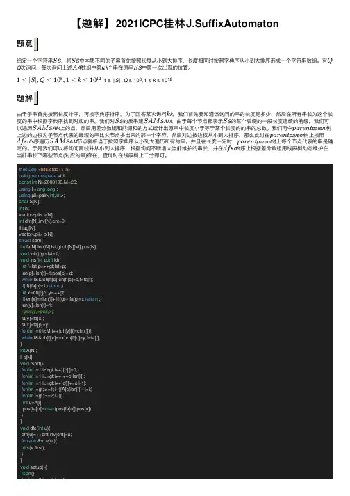
【题解】2021ICPC 桂林J.SuffixAutomaton题意给定⼀个字符串S ，将S 中本质不同的⼦串⾸先按照长度从⼩到⼤排序，长度相同时按照字典序从⼩到⼤排序形成⼀个字符串数组。

有Q 次询问，每次询问上述A 数组中第k 个串在原串S 中第⼀次出现的位置。

1≤|S |,Q ≤106,1≤k ≤1012题解由于⼦串⾸先按照长度排序，再按字典序排序，为了回答某次询问k ，我们⾸先要知道该询问的串的长度是多少，然后在所有串长为这个长度的串中根据字典序找到对应的串。

我们对S 的反串建SAM ，由于每个节点都表⽰S 的某个后缀的⼀段长度连续的前缀，我们可以遍历SAM 上的点，然后⽤差分数组和前缀和的⽅式统计出原串中长度⼩于等于某个长度的的串的总数。

我们再令parent 树上边的边权为⼦节点代表的最短的串⽐⽗节点多出来的那⼀个字符，然后对边按边权从⼩到⼤排序，那么此时在parent 树上按照dfs 序遍历SAM 节点就相当于按照字典序从⼩到⼤遍历所有的串。

并且在长度⼀定时，parent 树上每个节点代表的串是确定的。

于是我们可以将询问离线并从⼩到⼤排序，根据询问不断增⼤当前维护的串长，并在dfs 序上根据差分数组⽤线段树动态维护在当前串长下哪些节点(对应的串)存在，查询时在线段树上⼆分即可。

#include <bits/stdc++.h>using namespace std;const int N=2000100,M=26;using ll=long long ;using pii=pair<int ,int >;char S[N];int n;vector<pii> e[N];int dfn[N],inv[N],cnt=0;ll tag[N];vector<pii> b[N];struct sam{int fa[N],len[N],lst,gt,ch[N][M],pos[N];void init(){gt=lst=1;}void ins(int c,int id){int f=lst,p=++gt;lst=p;len[p]=len[f]+1;pos[p]=id;while (f&&!ch[f][c])ch[f][c]=p,f=fa[f];if (!f){fa[p]=1;return ;}int x=ch[f][c],y=++gt;if (len[x]==len[f]+1){gt--;fa[p]=x;return ;}len[y]=len[f]+1;//pos[y]=pos[x];fa[y]=fa[x];fa[x]=fa[p]=y;for (int i=0;i<M;i++)ch[y][i]=ch[x][i];while (f&&ch[f][c]==x)ch[f][c]=y,f=fa[f];}int A[N];ll c[N];void rsort(){for (int i=1;i<=gt;i++){c[i]=0;}for (int i=1;i<=gt;i++)++c[len[i]];for (int i=1;i<=gt;i++)c[i]+=c[i -1];for (int i=gt;i>=1;i--){A[c[len[i]]--]=i;}for (int i=gt;i>=2;i--){int u=A[i];pos[fa[u]]=max (pos[fa[u]],pos[u]);}}void dfs(int u){dfn[u]=++cnt;inv[cnt]=u;for (auto &v :e[u]){dfs (v.first);}}void setup(){rsort ();for (int i=2;i<=gt;i++){S S Q A k S 1≤|S |,Q ≤,1≤k ≤1061012k S SAM S SAM parent parent dfs SAM parent dfsfor(int i=2;i<=gt;i++){e[fa[i]].push_back(pii{i,S[pos[i]-len[fa[i]]]-'a'});}for(int i=1;i<=gt;i++){sort(e[i].begin(),e[i].end(),[&](const pii&a,const pii& b){return a.second<b.second;});}dfs(1);for(int i=2;i<=gt;i++){++tag[len[fa[i]]+1];--tag[len[i]+1];b[len[fa[i]]+1].push_back(pii{i,1});b[len[i]+1].push_back(pii{i,-1});}tag[0]=0;for(int i=1;i<=n;i++){tag[i]+=tag[i-1];}for(int i=1;i<=n;i++){tag[i]+=tag[i-1];}}}g;#define ls o<<1#define rs o<<1|1#define mid ((l+r)/2)int s[N<<2];void mt(int o){s[o]=s[ls]+s[rs];}void bd(int o,int l,int r){s[o]=0;if(l==r)return ;bd(ls,l,mid);bd(rs,mid+1,r);}void upd(int o,int l,int r,int x,int d){s[o]+=d;if(l==r)return ;if(x<=mid)upd(ls,l,mid,x,d);else upd(rs,mid+1,r,x,d);}int query(int o,int l,int r,int k){if(l==r)return l;return s[ls]>=k?query(ls,l,mid,k):query(rs,mid+1,r,k-s[ls]);}pair<ll,int> qu[N];pii ans[N];void f1(){scanf("%s",S+1);n=strlen(S+1);for(int i=1;i<=n/2;i++)swap(S[i],S[n-i+1]);g.init();for(int i=1;i<=n;i++){g.ins(S[i]-'a',i);}g.setup();int Q;scanf("%d",&Q);for(int i=1;i<=Q;i++){scanf("%lld",&qu[i].first);qu[i].second=i;}sort(qu+1,qu+1+Q,[&](const pair<ll,int>& a,const pair<ll,int>& b){ return a.first<b.first;});bd(1,1,g.gt);int na=1;for(int i=1;i<=Q;i++){ll k=qu[i].first;int id=qu[i].second;int np=lower_bound(tag+1,tag+1+n,k)-tag;if(np>n){ans[id]=pii{-1,-1};continue;}ll res=k-tag[np-1];while(na<=np){for(auto& v:b[na]){for(auto& v:b[na]){if(v.second==1){upd(1,1,g.gt,dfn[v.first],1);}else{upd(1,1,g.gt,dfn[v.first],-1);}}++na;}int nb=query(1,1,g.gt,res);nb=inv[nb];ans[id]=pii{n-g.pos[nb]+1,n-(g.pos[nb]-np+1)+1};}for(int i=1;i<=Q;i++){printf("%d %d\n",ans[i].first,ans[i].second);} }int main(){f1();return0;}。

J.Symbolic Computation(2001)31,259–276doi:10.1006/jsco.1999.1015Available online at onAn Optimal Algorithm for Constructing the Reduced Gr¨o bner Basis of Binomial Ideals,and Applications toCommutative SemigroupsULLA KOPPENHAGEN†AND ERNST W.MAYR†Institut f¨u r Informatik,Technische Universit¨a t M¨u nchen,D-80290M¨u nchen,GermanyIt is known that the reduced Gr¨o bner basis of general polynomial ideals can be computedin exponential space.The algorithm,obtained by K¨u hnle and Mayr,is,however,basedon rather complex parallel computations,and,above that,makes extensive use of theparallel computation thesis.In this paper,we exhibit an exponential space algorithmfor generating the reduced Gr¨o bner basis of binomial ideals which can be implementedwithout any complex parallel computations.This result is then applied to derive spaceoptimal decision procedures for thefinite enumeration and subword problems for com-mutative semigroups.c 2001Academic Press1.IntroductionThe method of Gr¨o bner bases(see Buchberger,1965;also Hironaka,1964)is a technique that provides algorithmic solutions to a variety of problems,for instance,primary decom-position of polynomial ideals,computations in the residue class ring modulo a polynomial ideal,decisions about various properties of ideals generated by a givenfinite set of poly-nomials,word problems modulo ideals and in commutative semigroups(reversible Petri nets),bijective enumeration of all polynomial ideals over a given coefficient domain etc. Although versions of Buchberger’s algorithm have been somewhat successful in prac-tice,the complexity of the algorithm is not well understood.Afirst step in understanding the complexity of the algorithm is to bound the degree of polynomials that occur in a minimal Gr¨o bner basis.In the univariate case,the Gr¨o bner-basis algorithm specializes to Euclid’s algorithm whose complexity has been extensively studied(see Loos,1982,for a survey).In the bi-variate case Buchberger(1983)and Lazard(1983)gave important bounds on the degrees and the number of polynomials occurring in a reduced Gr¨o bner basis.In the multivariate case,first steps towards an upper bound for the degrees in a minimal Gr¨o bner basis were taken in Bayer(1982)and M¨o ller and Mora(1984).However,these results did not,or only under very restrictive assumptions,imply bounds for the degree of the polynomials arising during the intermediate computations of the Gr¨o bner basis algorithms.Using a novel partitioning method for polynomial ideals,Dub´e(1990)obtained the †E-mail:{koppenha|mayr}@in.tum.de,rmatik.tu-muenchen.de/0747–7171/01/010259+18$35.00/0c 2001Academic Press260U.Koppenhagen and E.W.Mayrsharpened degree bound of2· d2+d 2k−1(with d the maximum degree of the input basis and k the number of indeterminates)for the degree of polynomials in a reduced Gr¨o bner basis,employing only combinatorial arguments.An exponential bound on the degrees of Gr¨o bner bases for zero-dimensional ideals was shown by Caniglia et al.(1988).Extending this result,Krick and Logar(1991) showed that Gr¨o bner bases of zero-or one-dimensional ideals can be computed in time exponential in the number of indeterminates.By transforming a representation of the normal form of a polynomial into a system of linear equations,K¨u hnle and Mayr(1996)exhibited an exponential space computation of Gr¨o bner bases.This algorithm,however,is based on rather complex parallel compu-tations like parallel rank computations of matrices,and,above that,makes extensive use of the parallel computation thesis(Fortune and Wyllie,1978).In this paper we present an exponential space algorithm for constructing the reduced Gr¨o bner basis of a binomial ideal(each generator is a difference of two terms;for an investigation of the algebraic structure of binomial ideals see Eisenbud and Sturmfels, 1996).This algorithm can be implemented without any difficult parallel rank compu-tations of matrices,or any other complex parallel computations.We make use of the close relationship between commutative semigroups and binomial ideals,in particular,of the algorithm in Mayr and Meyer(1982)for the uniform word problem in commutative semigroups.By the results in Mayr and Meyer(1982)and Huynh(1986),this algorithm is space optimal.As applications of this algorithm we derive a procedure enumerating the elements of finite congruence classes in commutative semigroups and an algorithm for the general subword problem in commutative semigroups.Both algorithms use exponential space and are space optimal.Another immediate application is computing complete rewrite systems for which we also obtain an exponential space completeness result(Huynh,1986).2.Basic Concepts and NotationsIn this section we review some definitions and notations used in the following.2.1.semigroups,Thue systems,and semigroup presentationsA semigroup(H,◦)is a set H with a binary operation◦which is associative.If ad-ditionally◦is commutative we have a commutative semigroup,and a semigroup with a unit element is called a monoid.For simplicity,we write ab instead of a◦b.A commutative monoid M is said to befinitely generated by afinite subset X= {x1,...,x k}⊆M if†M={u|u=x1 (x1)e k,e i∈N,x i∈X}.e2...x k...x ke1x2 (x2)Each element of M can then be represented as a k-dimensional vector in N k,i.e.there is a surjectionϕ:N k→M such thatϕ(e1,...,e k)=x1 (x1)e k.e2...x k...x ke1x2 (x2)†N denotes the set of non-negative integers,and Q the set of rationals.An Optimal Gr¨o bner Base Algorithm for Binomial Ideals,and Applications261 Ifϕis also injective,and hence bijective,then every element of M has a unique repre-sentation in N k,and M is said to be free.For afinite alphabet X={x1,...,x k},X denotes the free commutative monoid generated by X.LetΦ:X →N k be the so-called Parikh mapping,i.e.(Φ(u))i(also writtenΦ(u,x i)) indicates,for every u∈X and i∈{1,...,k},the number of occurrences of x i∈X in u. For an element u of X ,called a(commutative)word,the order of the symbols isimmaterial,and in the following we shall use an exponent notation:u=x e11...x e kk ,where e i=Φ(u,x i)∈N for i=1,...,k.A commutative semi-Thue system over X is given by afinite set P of productions l i→r i,where l i,r i∈X .A word v∈X is derived in one step from u∈X (written u→v(P))by application of the production(l i→r i)∈P iff,for some w∈X ,we have u=wl i and v=wr i.The word u derives v iffu∗→v(P),where∗→is the reflexive transitive closure of→.More precisely we write u+→v(P),where+→is the transitive closure of→,if u∗→v(P)and u=v.A sequence(u0,...,u n)of words u i∈X with u i→u i+1(P)for i=0,...,n−1is called a derivation(of length n)of u n from u0in P.A commutative Thue system is a symmetric commutative semi-Thue system P,i.e.(l→r)∈P⇒(r→l)∈P.Derivability in a commutative Thue system establishes a congruence≡P on X by the ruleu≡v mod P⇔d ef u∗→v(P).Thus,for commutative Thue systems,we also use the notation l≡r mod P to denote the pair of productions(l→r)and(r→l)in P.A commutative Thue system P is also called a presentation of the commutative quotient semigroup X /≡P.We note that commutative semi-Thue systems appear in other,equivalent formula-tions in the literature,like vector addition systems and Petri nets.Finitely presented commutative semigroups are equivalent to reversible vector addition systems or Petri nets.Readers more familiar with reversible Petri nets may want to think of a vector in N k as a marking.2.2.polynomials and idealsLet X denote thefinite set{x1,...,x k},and Q[X]the(commutative)ring of polyno-mials with indeterminates x1,...,x k and rational coefficients.A term t in x1,...,x k is a product of the form t=x e11·x e22···x e k k,with e=(e1,e2,...,e k)∈N k the degree vector of t.By the degree deg(t)of a term t we shall mean the integer e1+e2+···+e k(which is ≥0).Each polynomial f(x1,...,x k)∈Q[X]is afinite sum f(x1,...,x k)= n i=1a i·t i, with a i∈Q−{0}the coefficient of the i th term t i of f.The product m i=a i·t i is called the i th monomial of the polynomial f.The degree of a polynomial is the maximum of the degrees of its terms.An ideal in Q[X]is any subset I of Q[X]satisfying the following conditions:(I1)p,q∈I⇒p+q∈I;(I2)r∈Q[X],p∈I⇒r·p∈I.For f1,...,f h∈Q[X], f1,...,f h ⊆Q[X]denotes the ideal generated by{f1,...,f h},262U.Koppenhagen and E.W.Mayr that is†f1,...,f h :=hi=1p i f i;p i∈Q[X]for i∈I h.If I= f1,...,f h ,{f1,...,f h}is called a basis of I.An admissible term ordering≺on Q[X]is given by any admissible order on N k,i.e. any total order<on N k satisfying the following two conditions:(T1)e>(0,...,0)for all e∈N k−{(0,...,0)};(T2)a<b⇒a+c<b+c for all a,b,c∈N k.If(d1,...,d k)>(e1,...,e k),we say that any monomial a1·x d11···x d k k,a1∈Q−{0},is greater in the term ordering than any monomial a2·x e11···x e k k,a2∈Q−{0}(written a1·x d11···x d k k a2·x e11···x e k k).For a polynomial f(x1,...,x k)= n i=1a i·t i we always assume that t1 t2 ··· t n. For any such non-zero polynomial f∈Q[X]we define the leading term LT(f):=t1. For the sake of constructiveness,we assume that the term ordering is given as part of the input by a k×k integer matrix T such that a1·x d11···x d k k a2·x e11···x e k k iff,for the corresponding degree vectors d and e,T d is lexicographically greater than T e(see Robbiano,1985;Weispfenning,1987)Let I be an ideal in Q[X],and let some admissible term ordering≺on Q[X]be given.A finite set{g1,...,g r}of polynomials from Q[X]is called a Gr¨o bner basis of I(w.r.t.≺),if (G1){g1,...,g r}is a basis of I;(G2){LT(g1),...,LT(g r)}is a basis of the leading term ideal of I,which is the smallest ideal⊆Q[X]containing the leading terms of all f∈I,or equivalently:if f∈I,then LT(f)∈ LT(g1),...,LT(g r) .A Gr¨o bner basis is called reduced if no monomial in any one of its polynomials is divisible by the leading term of any other polynomial in the basis.3.The Connection between Commutative Semigroups and Binomial Ideals3.1.the basic problems and their relationshipIn this section,we consider the uniform word problem for commutative semigroups and the polynomial ideal membership problem.We will show the relationship between these two very basic and fundamental algorithmic problems for commutative semigroups and polynomial ideals.Let P={l i≡r i;i∈I h}be some(finite)commutative semigroup presentation with l i,r i∈X for i∈I h.We identify any u∈X (resp.the corresponding vectoru=(Φ(u,x1),...,Φ(u,x k))∈N k)with the term u=xΦ(u,x1)1·xΦ(u,x2)2···xΦ(u,x k)kandvice versa any term u=x e11·x e22···x e k k∈Q[X]with the wordu=x1 (x1)e1x2 (x2)e2...x k...x ke k∈X .†For n∈N,I n denotes the set{1,...,n}.An Optimal Gr¨o bner Base Algorithm for Binomial Ideals,and Applications263 By I(P)we denote the Q[X]-ideal generated by{l1−r1,...,l h−r h},i.e.I(P):=hi=1p i(l i−r i);p i∈Q[X]for i∈I h.We call such an ideal a binomial ideal,i.e.each polynomial in the basis is the difference of two terms.By looking at Buchberger’s(1965)algorithm it is not hard to see that the reduced Gr¨o bner basis of a binomial ideal still consists only of binomials.The Uniform Word Problem for commutative semigroups is:Given a commutative semi-group presentation P over some alphabet X,and two words u,v∈X ,decide whether u≡v mod P.The Polynomial Ideal Membership Problem is:Given polynomials f,f1,...,f h∈Q[X], decide whether f∈ f1,...,f h .Proposition3.1.(Mayr and Meyer,1982)Let X={x1,...,x k},P={l i≡r i; l i,r i∈X ,i∈I h},and u,v∈X .Then the following are equivalent:(i)there exist p1,...,p h∈Q[X]such that v−u= h i=1p i(l i−r i);(ii)there is a derivation u=γ1→γ2→...→γn=v(P)of v from u in P such that for j∈I n deg(γj)≤max{deg(l i p i),deg(r i p i);i∈I h};(iii)u≡v mod P.In the fundamental paper(Hermann,1926),G.Hermann gave a doubly exponential degree bound for the polynomial ideal membership problem:Proposition3.2.(Hermann,1926)Let X={x1,...,x k},g,g1,...,g h∈Q[X],and d:=max{deg(g i);i∈I h}.If g∈ g1,...,g h ,then there exist p1,...,p h∈Q[X]such that(i)g= h i=1g i p i;(ii)(∀i∈I h);[deg(p i)≤deg(g)+(hd)2k].By size(·)we shall denote the number of bits needed to encode the argument in some standard way(using radix representation for numbers).Then the above two propositions yield an exponential space upper bound for the uniform word problem for commutative semigroups:Proposition3.3.(Mayr and Meyer,1982)Let X={x1,...,x k}and P={l i≡r i;l i,r i∈X ,i∈I h}.Then there is a(deterministic)Turing machine M and some constant c>0independent of P,such that M decides for any two words u,v∈X whether u≡v mod P using at most space(size(u,v,P))2·2c·k.3.2.the reduced Gr¨o bner basis for binomial idealsLet P be a commutative semigroup presentation over some alphabet X,and≺some admissible term ordering on Q[X].The following two theorems characterize the binomials of the reduced Gr¨o bner basis of I(P)(w.r.t.≺).Thefirst shows that in each binomial of264U.Koppenhagen and E.W.Mayrthe reduced Gr¨o bner basis G of I(P)the smaller term(w.r.t.≺)is the minimal element (w.r.t.≺)of the congruence class of the leading term.Theorem3.1.Let X={x1,...,x k},P={l i≡r i;l i,r i∈X ,i∈I h},and G={h1−m1,...,h r−m r}be the reduced Gr¨o bner basis of the ideal I(P)w.r.t.some admissible term ordering≺(m i≺h i).Then m i is the minimal element(w.r.t.≺)of the congruence class[h i]P,i∈I r.Proof.Assume that w=m i is the minimal element of[h i]P(w.r.t.≺).Then w≺m i and m i−w∈I(P).Since G is a Gr¨o bner basis of I(P),m i∈ h1,...,h r ,i.e.there must be some j∈I r such that h j divides m i.This however contradicts the fact that h i−m i is an element of the reduced Gr¨o bner basis of I(P).2The next theorem characterizes the leading terms of the polynomials in I(P). Theorem3.2.Let X={x1,...,x k},P={l i≡r i;l i,r i∈X ,i∈I h},and G={h1−m1,...,h r−m r}be the reduced Gr¨o bner basis of the ideal I(P)w.r.t.some admissible term ordering≺(m i≺h i).Then LT(I(P))(the set of the leading terms of I(P))is the set of all terms with non-trivial congruence class which are not the minimal element in their congruence class w.r.t.≺.H={h1,...,h r}is the set of the minimal elements of LT(I(P))w.r.t.divisibility.Proof.Since G is the reduced Gr¨o bner basis of I(P),it is clear that H is the set of the minimal elements of LT(I(P))w.r.t.divisibility.Since h i−m i∈I(P),there is a derivation in P of m i≺h i from h i(h i+→m i(P)),for all i∈I r.Because G is a Gr¨o bner basis,for any h∈LT(I(P))there is an h j−m j∈G and a term t in X with h=t·h j and h+→t·m j(P).Thus,for any h∈LT(I(P)),the congruence class[h]P is non-trivial,and h is not the minimal element in[h]P.Let s∈X be a term with non-trivial congruence class.If s is not the minimal element m s(w.r.t.≺)of its congruence class[s]P,then s derives m s(s+→m s(P)),and thus, s−m s∈I(P),i.e.s∈LT(I(P)).If s=m s,then there is no derivation of any t s≺s from s,and there is no h j∈H such that h j divides s.This is because if there is some h j∈H and some term t in X with s=t·h j,then s≡t·m j mod P what contradicts the minimality of s.Thus,if s=m s,then s∈LT(I(P))and s∈H.24.An Optimal Algorithm for the Reduced Gr¨o bner BasisIn this section we give an exponential space algorithm for generating the reduced Gr¨o bner basis of a binomial ideal.To determine the complexity of the algorithm we need the results of Section3and the following upper bound for the total degree of polynomials required in a Gr¨o bner basis,obtained by Dub´e(1990).Note that we use exponential notation in representing words over X.Proposition4.1.(Dub´e,1990)Let X={x1,...,x k},F={f1,...,f h}⊂Q[X], I= f1,...,f h the ideal generated by F,and let d be the maximum degree of any f∈F. Then,for any admissible term ordering≺on Q[X],the degree of polynomials required in a Gr¨o bner basis for I w.r.t.≺is bounded by2· d2+d 2k−1.An Optimal Gr¨o bner Base Algorithm for Binomial Ideals,and Applications265 Now we will generate the reduced Gr¨o bner basis of the binomial ideal I(P)w.r.t.some fixed admissible term ordering≺,where X={x1,...,x k}and P={l i≡r i;l i,r i∈X ,i∈I h}(w.l.o.g.l i r i).Let H denote the set{h1,...,h r}of the minimal elements of LT(I(P))w.r.t.divisibility,and m i the minimal element of[h i]P w.r.t.≺,for i∈I r. From Theorems3.1and3.2we know that the set G={h1−m1,...,h r−m r}is the reduced Gr¨o bner basis of I(P).We have to determine the elements in H,as well as the minimal element m i(w.r.t.≺) of the congruence class of each h i∈H.From Proposition4.1we know that the degrees deg(h i)and deg(m i)are bounded by2· d22+d 2k−1,where d is the maximum degree of any l i−r i,i∈I h.Lemma4.1.For a term u∈X with non-trivial congruence class the minimal element w.r.t.≺of[u]P is of the form t·r i with r i∈{r1,...,r h},t∈X .Proof.W.l.o.g.assume that u is not the minimal element m u of[u]P w.r.t.≺.Then there is a derivation in P leading from u to m u≺u,i.e.u+→m u(P),where m u=t·r i for some r i∈{r1,...,r h},t∈X (note that l j r j∀j∈I h).2···x e k k. For h=x e11···x e k k∈X and i∈I k such that e i≥1,define h(i):=x e11···x e i−1i Then H consists exactly of those terms h∈X which have degree≤2· d2+d 2k−1,which are congruent to some term t·r i≺h with r i∈{r1,...,r h},t∈X ,and deg(t·r i)≤2· d2+d 2k−1,and for which,for all applicable i,[h(i)]P is trivial.By Proposition3.3, the condition regarding the reducibility of h can be checked in space(size(P))2·2c·k for some constant c>0independent of P.Testing non-reducibility of the h(i)can also be done in exponential space because of Proposition3.3and:Lemma4.2.A term u∈X with deg(u)≤D is an element of LT(I(P))iffthere is some t·r i with t·r i≺u,r i∈{r1,...,r h},t∈X ,and deg(t·r i)≤D+2· d22+d 2k−1 such that u+→t·r i(P).Proof.We only have to prove the degree bound.Note that u∈LT(I(P))iffeither u∈H,and thus deg(m u)≤2· d22+d 2k−1,where m u is the minimal element of[u]P,or there is some h∈H with u=t u·h for some t u∈X .The degree of the minimal element m h of[h]P w.r.t.≺is bounded by2· d22+d 2k−1.From m h≺h we get t u·m h≺u with deg(t u·m h)≤D+2· d2+d 2k−1.2From this,we derive the exponential space algorithm given in Figure1.Putting everything together,we have proven the following theorem.Theorem4.1.Let X={x1,...,x k},P={l i≡r i;l i,r i∈X ,i∈I h},and≺some admissible term ordering.Then there is an algorithm which generates the reduced Gr¨o bner basis G={h1−m1,...,h r−m r}of the binomial ideal I(P)using at most space (size(P))2·2¯c·k≤2c·size(P),where¯c,c>0are some constants independent of P.266U.Koppenhagen and E.W.MayrThe AlgorithmInput:admissible term ordering≺,P={l1−r1,...,l h−r h}with r i≺l i∀i∈I h Output:the reduced Gr¨o bner basis G={h1−m1,...,h r−m r}of I(P)d:=max{deg(l i),deg(r i);i∈I h}G:=∅for each h=x e11···x e k k∈X with degree≤2· d22+d 2k−1dogb:=falseif there exists t·r i with t·r i≺h,r i∈{r1,...,r h},t∈X ,deg(t·r i)≤2· d22+d 2k−1 which is≡h mod P then/*h∈LT(I(P))*/m:=the minimal(w.r.t.≺)among these termsgb:=trueend ifD:=deg(h)for each i∈I k with e i≥1while gb doh :=x e11···x e i−1i···x e k kif there exists t·r j with t·r j≺h ,r j∈{r1,...,r h},t∈X ,deg(t·r j)≤(D−1)+2· d22+d 2k−1which is≡h mod P then/*h ∈LT(I(P))⇒h∈H*/gb:=falseend ifend forif gb then/*h∈H*/G:=G∪{h−m}end ifend forFigure1.Algorithm for constructing the reduced Gr¨o bner basis of a binomial ideal.From the results in Huynh(1986)we know that,in the worst case,any Gr¨o bner basis of I(P)has maximal degree at least22c ·size(P)for some constant c >0independent of P. Hence,any algorithm that computes Gr¨o bner bases of binomial ideals requires at least exponential space in the worst case.5.ApplicationsWe now consider two applications of the exponential space algorithm obtained in Sec-tion4.We present space optimal decision procedures for thefinite enumeration and subword problems for commutative semigroups.5.1.the finite enumeration problem for commutative semigroupsLet P be afinite commutative semigroup presentation over some alphabet X,and u∈X a word such that the congruence class of u isfinite(or,synonymously,bounded).Then thefinite enumeration problem for commutative semigroups,or equivalently,reversibleAn Optimal Gr¨o bner Base Algorithm for Binomial Ideals,and Applications267Petri nets is the problem of generating a complete list of all the elements of[u]P.We give a procedure for the solution of this problem which needs at most exponential work space.Theorem5.1.Let X={x1,...,x k},P={l i≡r i;l i,r i∈X ,i∈I h}be afinite commutative semigroup presentation over X,and u∈X a word such that the congruence class of u isfinite.Then there is an algorithm which generates the elements of[u]P using at most space(size(u,P))2·2¯c·k≤2c·size(u,P),where¯c,c>0are some constants independent of u and P.Proof.In addition to x1,...,x k we introduce2k+3new variables m,s,t,y1,...,y k and z1,...,z k.Let X =X∪{m,s,t,y1,...,y k,z1,...,z k}.Given P and the word u∈X ,we construct a new commutative semigroup presentation P over X as follows:P contains the relationss·x j≡s·y j·z j,for j=1,...,k,(5.1)s·y(u)≡t,(5.2)s·u≡m,(5.3) and,for every relation l i≡r i in P,the relations·y(l i)≡s·y(r i),and(5.4)t·z(l i)≡t·z(r i),(5.5) where y,resp.z are the homomorphisms replacing x j by y j,resp.z j,j∈I k.Let≺be a lexicographic term ordering satisfyingm≺a≺s≺b for all a∈{x1,...,x k},b∈{t,y1,...,y k,z1,...,z k}.In the following we prove that v∈[u]P iffs·v−m∈G,where G is the reduced Gr¨o bner basis of the ideal I(P )w.r.t.≺.Then,by Theorem4.1,the elements of[u]P can be generated using at most space(size(u,P ))2·2d ·k≤(size(u,P))2·2d·k,where d ,d>0 are some constants independent of u and P ,resp.P.First we establish some technical details.Lemma5.1.Every word w∈[s·u]P satisfies the following conditions:(i)Φ(w,s)+Φ(w,t)+Φ(w,m)=1;(ii)ifΦ(w,s)=1,then xΦ(w,x1)+Φ(w,y1)1·xΦ(w,x2)+Φ(w,y2)2···xΦ(w,x k)+Φ(w,y k)k∈[u]P,xΦ(w,x1)+Φ(w,z1) 1·xΦ(w,x2)+Φ(w,z2)2···xΦ(w,x k)+Φ(w,z k)k∈[u]P;ifΦ(w,t)=1,thenΦ(w,x1)=Φ(w,x2)=...=Φ(w,x k)=0,Φ(w,y1)=Φ(w,y2)=...=Φ(w,y k)=0,xΦ(w,z1) 1·xΦ(w,z2)2···xΦ(w,z k)k∈[u]P.Proof.Let w be any word in[s·u]P .Then there is a repetition-free derivation in P leading from s·u to w.If w=m,then w is derived in one step from s·u by relation(5.3) and w trivially satisfies conditions(i)and(ii).Note that if in a derivation starting at s·u relation(5.3)is applied,then this derivation can only be continued by again using268U.Koppenhagen and E.W.Mayrrelation (5.3),causing a repetition.If w =m ,then in any repetition-free derivation starting at s ·u leading to w only the relations in (5.1)and (5.4)can be applied until the word s ·y (u )·z (u )is reached and changed to t ·z (u )by relation (5.2).Since [u ]P is finite,there is no u ∈{y 1,...,y k } with s ·u ·z (u )∈[s ·u ]P ,u =y (u ),and y (u )divides u .Therefore,any word w occurring in this derivation of s ·y (u )·z (u )from s ·u satisfies conditions (i)and (ii):(i)Φ(w,s )=1,Φ(w,t )=0,Φ(w,m )=0,(ii)x Φ(w,x 1)+Φ(w,y 1)1·x Φ(w,x 2)+Φ(w,y 2)2···x Φ(w,x k )+Φ(w,y k )k ∈[u ]P ,and x Φ(w,x 1)+Φ(w,z 1)1·x Φ(w,x 2)+Φ(w,z 2)2···x Φ(w,x k )+Φ(w,z k )k =u .Then,as long as relation (5.2)is not applied,by the relations in (5.5),words t ·z (v )with v ∈[u ]P can be derived from t ·z (u ).Note that for all such words t ·z (v )with v ∈[u ]P Φ(t ·z (v ),s )=0,Φ(t ·z (v ),t )=1,Φ(t ·z (v ),m )=0,and condition (ii)is satisfied.Relation (5.2)changes t ·z (v )to s ·y (u )·z (v )and again the relations in (5.1)and (5.4)can be applied.As above,the words w in the resulting sub-derivation starting at s ·y (u )·z (v )satisfy (i)and (ii)withx Φ(w,x 1)+Φ(w,z 1)1·x Φ(w,x 2)+Φ(w,z 2)2···x Φ(w,x k )+Φ(w,z k )k =v.By the relations in (5.4),from s ·y (u )·z (v )any word s ·y (v )·z (v )with v ∈[u ]P can be derived.Relation (5.2)can only be applied to the word s ·y (u )·z (v ),causing a repetition.Thus,conditions (i)and (ii)are satisfied within the whole derivation.This completes the proof of Lemma 5.1.2For the derivation of some word s ·v ∈[s ·u ]P ,with v ∈X ,from s ·u in P we conclude from Lemma 5.1and its proof:Corollary 5.1.Let s ·v ∈[s ·u ]P with v ∈X ,v =u ,and let s ·u =γ0→γ1→···→γn =s ·v be any repetition-free derivation in P leading from s ·u to s ·v .Then there is exactly one i ∈I n −1with γi =s ·y (u )·z (u ),γi +1=t ·z (u ),and exactly one j ∈I n −1,j >i ,with γj =t ·z (v ),γj +1=s ·y (u )·z (v ).Thus,we can prove:Lemma 5.2.Let v be some word in X ,thenv ∈[u ]P ⇐⇒s ·v ∈[s ·u ]P .Proof.By Lemma 5.1and its Corollary 5.1,a repetition-free derivation in P leading from s ·u to s ·v with v ∈X has the following form:s ·u +−→(5.1),(5.4)s ·y (u )·z (u )−→(5.2)t ·z (u )+−→(5.5)t ·z (v )−→(5.2)s ·y (u )·z (v )+−→(5.1),(5.4)s ·v,where +−→(.)denotes some repetition-free derivation applying only the relations given in (.).Within the sub-derivations +−→(5.1),(5.4),the values Φ(w,x i )+Φ(w,z i )are constantAn Optimal Gr¨o bner Base Algorithm for Binomial Ideals,and Applications 269for all i ∈I k ,i.e.the word x Φ(w,x 1)+Φ(w,z 1)1·x Φ(w,x 2)+Φ(w,z 2)2···x Φ(w,x k )+Φ(w,z k )kremainsthe same within +−→(5.1),(5.4).Furthermore,all words occurring in the above derivationsatisfy Lemma 5.1.2Lemma 5.3.[s ·u ]P is finite.Proof.Since [u ]P is finite,it follows from the definition of P and Lemma 5.1that[s ·u ]P is also finite.2Lemma 5.4.Let v be some word in X with v ∈[u ]P ,and v divides some u ∈[u ]P .Then s ·v is the minimal (w.r.t.≺)element of its congruence class [s ·v ]P .Proof.If v ∈X with v ∈[u ]P ,and v divides some u ∈[u ]P ,then there is some v ∈X −{ε}with u =v ·v ∈[u ]P .Because of the finiteness of [u ]P there is no ¯v ∈[v ]Pwith ¯v =u ·¯u for ¯u ∈X .If there is such a ¯v ∈[v ]P ,then u =v ·v ≡¯v ·vmod P ,¯v ·v =u ·¯u ·v ∈[u ]P ,i.e.[u ]P is not finite.Thus,in any derivation starting at s ·v relations (5.2)and (5.3)cannot be applied.Only the relations in (5.1)and (5.4)can possibly be used.Since y i x i (resp.z i x i )for all i ∈I k ,s ·v is the minimal element of [s ·v ]P w.r.t.≺.2Note that each v ∈X is the minimal (w.r.t.≺)element of [v ]P because no relation in P is applicable.Since [s ·u ]P is finite,it follows from Dickson’s (1913)Lemma that each w ∈[s ·u ]P is minimal in [s ·u ]P w.r.t.divisibility,i.e.if w ∈[s ·u ]P ,then there is no w ∈[s ·u ]P ,w =w such that w divides w .The minimal element w.r.t.≺of [s ·u ]P is m .Thus,by Lemma 5.4,each s ·v ∈[s ·u ]P with v ∈X is contained in the set of the minimal elements of LT (I (P ))w.r.t.divisibility,and hence G ⊇{s ·v −m |s ·v ∈[s ·u ]P ,v ∈X }(see Theorems 3.1and 3.2).This establishes Theorem 5.1.2As an example of Theorem 5.1,consider the finite commutative semigroup presentationP ={x 21≡x 1x 32,x 22≡x 2x 33}over the alphabet X ={x 1,x 2,x 3}and the word u =x 31.Splitting each relation of P into its two corresponding productions providesx 21→x 1x 32,(5.1)x 1x 32→x 21,(5.2)x 22→x 2x 33,(5.3)x 2x 33→x 22.(5.4)Applying these productions,the congruence class [u ]P of u in P can be derived as shown in Figure 2(v 1(.)−→v 2means that v 2is derived in one step from v 1by application of production (.)).Note that [u ]P is finite.Using the construction of Theorem 5.1we compute the reduced Gr¨o bner basis G of the idealI := sy 1z 1−sx 1,sy 2z 2−sx 2,sy 3z 3−sx 3,。

F(n) = max{cn + F(n-2), F(n-1)} for n > 1,
F(0) = 0, F(1)=c₁
A. Levitin “Introduction to the Design & Analysis of Algorithms,” 3rd ed., Ch. 8 ©2012 Pearson Education, Inc. Upper Saddle River, NJ. All Rights Reserved.
Example 3: Path counting
Consider the problem of counting the number of shortest paths from point A to point B in a city with perfectly horizontal streets and vertical avenues
1
A
B
A. Levitin “Introduction to the Design & Analysis of Algorithms,” 3rd ed., Ch. 8 ©2012 Pearson Education, Inc. Upper Saddle River, NJ. All Rights Reserved.
A. Levitin “Introduction to the Design & Analysis of Algorithms,” 3rd ed., Ch. 8 ©2012 Pearson Education, Inc. Upper Saddle River, NJ. All Rights Reserved.
Dynamic Programming

has real (identical/different) or complex roots. (Use input command for entering the coefficients (a,b,c) of the equation and disp commands to display the output). The program can calculates the roots in each case.
executed.
The programmer can handle errors in the program without causing the program to stop.
29
Branches (try/catch)
30
Branches (try/catch)
Example
31
An Overview
3
m文件的类型
m文件有两类：独立的m文件 — 称命令文件 可调用m文件 — 称函数文件 （1） 命令文件 — 简单的m文件 命令文件实际上是一串指令的集合，与在命令窗口逐行 执行文件中的所有指令，其结果是一样的。没有输入输出 参数。 （2）matlab内置函数文件 matlab自定义的函数文件称内置函数文件。 （3）函数m文件— 需要输入变量，返回输出变量
matlab用户可以根据需要编辑自己的m文件，它们可以
像库函数一样方便的调用，从而极大地扩展了matlab 的 能力。 注：Matlab的函数极其使用将在第四章介绍）
4
第三章 MATLAB编程（分支和循环）
• Branching • Loops
5
Objectives（Branching and Loops）

Reprinted with corrections from The Bell System Technical Journal,V ol.27,pp.379–423,623–656,July,October,1948.A Mathematical Theory of CommunicationBy C.E.SHANNONI NTRODUCTIONHE recent development of various methods of modulation such as PCM and PPM which exchangebandwidth for signal-to-noise ratio has intensified the interest in a general theory of communication.A basis for such a theory is contained in the important papers of Nyquist1and Hartley2on this subject.In the present paper we will extend the theory to include a number of new factors,in particular the effect of noise in the channel,and the savings possible due to the statistical structure of the original message and due to the nature of thefinal destination of the information.The fundamental problem of communication is that of reproducing at one point either exactly or ap-proximately a message selected at another point.Frequently the messages have meaning;that is they refer to or are correlated according to some system with certain physical or conceptual entities.These semantic aspects of communication are irrelevant to the engineering problem.The significant aspect is that the actual message is one selected from a set of possible messages.The system must be designed to operate for each possible selection,not just the one which will actually be chosen since this is unknown at the time of design.If the number of messages in the set isfinite then this number or any monotonic function of this number can be regarded as a measure of the information produced when one message is chosen from the set,all choices being equally likely.As was pointed out by Hartley the most natural choice is the logarithmic function.Although this definition must be generalized considerably when we consider the influence of the statistics of the message and when we have a continuous range of messages,we will in all cases use an essentially logarithmic measure.The logarithmic measure is more convenient for various reasons:1.It is practically more useful.Parameters of engineering importance such as time,bandwidth,numberof relays,etc.,tend to vary linearly with the logarithm of the number of possibilities.For example,adding one relay to a group doubles the number of possible states of the relays.It adds1to the base2logarithm of this number.Doubling the time roughly squares the number of possible messages,ordoubles the logarithm,etc.2.It is nearer to our intuitive feeling as to the proper measure.This is closely related to(1)since we in-tuitively measures entities by linear comparison with common standards.One feels,for example,thattwo punched cards should have twice the capacity of one for information storage,and two identicalchannels twice the capacity of one for transmitting information.3.It is mathematically more suitable.Many of the limiting operations are simple in terms of the loga-rithm but would require clumsy restatement in terms of the number of possibilities.The choice of a logarithmic base corresponds to the choice of a unit for measuring information.If the base2is used the resulting units may be called binary digits,or more briefly bits,a word suggested by J.W.Tukey.A device with two stable positions,such as a relay or aflip-flop circuit,can store one bit of information.N such devices can store N bits,since the total number of possible states is2N and log22N N.If the base10is used the units may be called decimal digits.Sincelog2M log10M log102332log10M1Nyquist,H.,“Certain Factors Affecting Telegraph Speed,”Bell System Technical Journal,April1924,p.324;“Certain Topics in Telegraph Transmission Theory,”A.I.E.E.Trans.,v.47,April1928,p.617.2Hartley,R.V.L.,“Transmission of Information,”Bell System Technical Journal,July1928,p.535.INFORMATIONSOURCE TRANSMITTER RECEIVER DESTINATIONNOISE SOURCEFig.1—Schematic diagram of a general communication system.a decimal digit is about 313bits.A digit wheel on a desk computing machine has ten stable positions and therefore has a storage capacity of one decimal digit.In analytical work where integration and differentiation are involved the base e is sometimes useful.The resulting units of information will be called natural units.Change from the base a to baseb merely requires multiplication by log b a .By a communication system we will mean a system of the type indicated schematically in Fig.1.It consists of essentially five parts:1.An information source which produces a message or sequence of messages to be communicated to thereceiving terminal.The message may be of various types:(a)A sequence of letters as in a telegraph of teletype system;(b)A single function of time f t as in radio or telephony;(c)A function of time and other variables as in black and white television —here the message may be thought of as a function f x y t of two space coordinates and time,the light intensity at point x y and time t on a pickup tube plate;(d)Two or more functions of time,say f t ,g t ,h t —this is the case in “three-dimensional”sound transmission or if the system is intended to service several individual channels in multiplex;(e)Several functions of several variables —in color television the message consists of three functions f x y t ,g x y t ,h x y t defined in a three-dimensional continuum —we may also think of these three functions as components of a vector field defined in the region —similarly,several black and white television sources would produce “messages”consisting of a number of functions of three variables;(f)Various combinations also occur,for example in television with an associated audio channel.2.A transmitter which operates on the message in some way to produce a signal suitable for trans-mission over the channel.In telephony this operation consists merely of changing sound pressure into a proportional electrical current.In telegraphy we have an encoding operation which produces a sequence of dots,dashes and spaces on the channel corresponding to the message.In a multiplex PCM system the different speech functions must be sampled,compressed,quantized and encoded,and finally interleaved properly to construct the signal.V ocoder systems,television and frequency modulation are other examples of complex operations applied to the message to obtain the signal.3.The channel is merely the medium used to transmit the signal from transmitter to receiver.It may bea pair of wires,a coaxial cable,a band of radio frequencies,a beam of light,etc.4.The receiver ordinarily performs the inverse operation of that done by the transmitter,reconstructingthe message from the signal.5.The destination is the person (or thing)for whom the message is intended.We wish to consider certain general problems involving communication systems.To do this it is first necessary to represent the various elements involved as mathematical entities,suitably idealized from theirphysical counterparts.We may roughly classify communication systems into three main categories:discrete, continuous and mixed.By a discrete system we will mean one in which both the message and the signal are a sequence of discrete symbols.A typical case is telegraphy where the message is a sequence of lettersand the signal a sequence of dots,dashes and spaces.A continuous system is one in which the message and signal are both treated as continuous functions,e.g.,radio or television.A mixed system is one in which both discrete and continuous variables appear,e.g.,PCM transmission of speech.Wefirst consider the discrete case.This case has applications not only in communication theory,but also in the theory of computing machines,the design of telephone exchanges and otherfields.In additionthe discrete case forms a foundation for the continuous and mixed cases which will be treated in the second half of the paper.PART I:DISCRETE NOISELESS SYSTEMS1.T HE D ISCRETE N OISELESS C HANNELTeletype and telegraphy are two simple examples of a discrete channel for transmitting information.Gen-erally,a discrete channel will mean a system whereby a sequence of choices from afinite set of elementarysymbols S1S n can be transmitted from one point to another.Each of the symbols S i is assumed to have a certain duration in time t i seconds(not necessarily the same for different S i,for example the dots anddashes in telegraphy).It is not required that all possible sequences of the S i be capable of transmission on the system;certain sequences only may be allowed.These will be possible signals for the channel.Thus in telegraphy suppose the symbols are:(1)A dot,consisting of line closure for a unit of time and then line open for a unit of time;(2)A dash,consisting of three time units of closure and one unit open;(3)A letter space consisting of,say,three units of line open;(4)A word space of six units of line open.We might place the restriction on allowable sequences that no spaces follow each other(for if two letter spaces are adjacent, it is identical with a word space).The question we now consider is how one can measure the capacity of such a channel to transmit information.In the teletype case where all symbols are of the same duration,and any sequence of the32symbols is allowed the answer is easy.Each symbol representsfive bits of information.If the system transmits n symbols per second it is natural to say that the channel has a capacity of5n bits per second.This does not mean that the teletype channel will always be transmitting information at this rate—this is the maximum possible rate and whether or not the actual rate reaches this maximum depends on the source of information which feeds the channel,as will appear later.In the more general case with different lengths of symbols and constraints on the allowed sequences,we make the following definition:Definition:The capacity C of a discrete channel is given byC LimT∞log N TTwhere N T is the number of allowed signals of duration T.It is easily seen that in the teletype case this reduces to the previous result.It can be shown that the limit in question will exist as afinite number in most cases of interest.Suppose all sequences of the symbols S1S n are allowed and these symbols have durations t1t n.What is the channel capacity?If N t represents the number of sequences of duration t we haveN t N t t1N t t2N t t nThe total number is equal to the sum of the numbers of sequences ending in S1S2S n and these are N t t1N t t2N t t n,respectively.According to a well-known result infinite differences,N t is then asymptotic for large t to X t0where X0is the largest real solution of the characteristic equation:X t1X t2X t n1and thereforeC log X0In case there are restrictions on allowed sequences we may still often obtain a difference equation of this type andfind C from the characteristic equation.In the telegraphy case mentioned aboveN t N t2N t4N t5N t7N t8N t10as we see by counting sequences of symbols according to the last or next to the last symbol occurring. Hence C is log0where0is the positive root of12457810.Solving this wefind C0539.A very general type of restriction which may be placed on allowed sequences is the following:We imagine a number of possible states a1a2a m.For each state only certain symbols from the set S1S n can be transmitted(different subsets for the different states).When one of these has been transmitted the state changes to a new state depending both on the old state and the particular symbol transmitted.The telegraph case is a simple example of this.There are two states depending on whether or not a space was the last symbol transmitted.If so,then only a dot or a dash can be sent next and the state always changes. If not,any symbol can be transmitted and the state changes if a space is sent,otherwise it remains the same. The conditions can be indicated in a linear graph as shown in Fig.2.The junction points correspond totheFig.2—Graphical representation of the constraints on telegraph symbols.states and the lines indicate the symbols possible in a state and the resulting state.In Appendix1it is shown that if the conditions on allowed sequences can be described in this form C will exist and can be calculated in accordance with the following result:Theorem1:Let b s i j be the duration of the s th symbol which is allowable in state i and leads to state j. Then the channel capacity C is equal to log W where W is the largest real root of the determinant equation:∑s W bsi j i j0where i j1if i j and is zero otherwise.For example,in the telegraph case(Fig.2)the determinant is:1W2W4W3W6W2W410On expansion this leads to the equation given above for this case.2.T HE D ISCRETE S OURCE OF I NFORMATIONWe have seen that under very general conditions the logarithm of the number of possible signals in a discrete channel increases linearly with time.The capacity to transmit information can be specified by giving this rate of increase,the number of bits per second required to specify the particular signal used.We now consider the information source.How is an information source to be described mathematically, and how much information in bits per second is produced in a given source?The main point at issue is the effect of statistical knowledge about the source in reducing the required capacity of the channel,by the useof proper encoding of the information.In telegraphy,for example,the messages to be transmitted consist of sequences of letters.These sequences,however,are not completely random.In general,they form sentences and have the statistical structure of,say,English.The letter E occurs more frequently than Q,the sequence TH more frequently than XP,etc.The existence of this structure allows one to make a saving in time(or channel capacity)by properly encoding the message sequences into signal sequences.This is already done to a limited extent in telegraphy by using the shortest channel symbol,a dot,for the most common English letter E;while the infrequent letters,Q,X,Z are represented by longer sequences of dots and dashes.This idea is carried still further in certain commercial codes where common words and phrases are represented by four-orfive-letter code groups with a considerable saving in average time.The standardized greeting and anniversary telegrams now in use extend this to the point of encoding a sentence or two into a relatively short sequence of numbers.We can think of a discrete source as generating the message,symbol by symbol.It will choose succes-sive symbols according to certain probabilities depending,in general,on preceding choices as well as the particular symbols in question.A physical system,or a mathematical model of a system which produces such a sequence of symbols governed by a set of probabilities,is known as a stochastic process.3We may consider a discrete source,therefore,to be represented by a stochastic process.Conversely,any stochastic process which produces a discrete sequence of symbols chosen from afinite set may be considered a discrete source.This will include such cases as:1.Natural written languages such as English,German,Chinese.2.Continuous information sources that have been rendered discrete by some quantizing process.Forexample,the quantized speech from a PCM transmitter,or a quantized television signal.3.Mathematical cases where we merely define abstractly a stochastic process which generates a se-quence of symbols.The following are examples of this last type of source.(A)Suppose we havefive letters A,B,C,D,E which are chosen each with probability.2,successivechoices being independent.This would lead to a sequence of which the following is a typicalexample.B DC B C E C C C AD C B D D A AE C E E AA B B D A E E C A C E E B A E E C B C E A D.This was constructed with the use of a table of random numbers.4(B)Using the samefive letters let the probabilities be.4,.1,.2,.2,.1,respectively,with successivechoices independent.A typical message from this source is then:A A A C D CB DC E A AD A D A CE D AE A D C A B E D A D D C E C A A A A A D.(C)A more complicated structure is obtained if successive symbols are not chosen independentlybut their probabilities depend on preceding letters.In the simplest case of this type a choicedepends only on the preceding letter and not on ones before that.The statistical structure canthen be described by a set of transition probabilities p i j,the probability that letter i is followedby letter j.The indices i and j range over all the possible symbols.A second equivalent way ofspecifying the structure is to give the“digram”probabilities p i j,i.e.,the relative frequency ofthe digram i j.The letter frequencies p i,(the probability of letter i),the transition probabilities 3See,for example,S.Chandrasekhar,“Stochastic Problems in Physics and Astronomy,”Reviews of Modern Physics,v.15,No.1, January1943,p.1.4Kendall and Smith,Tables of Random Sampling Numbers,Cambridge,1939.p i j and the digram probabilities p i j are related by the following formulas:p i∑j p i j∑jp j i∑jp j p j ip i j p i p i j∑j p i j∑ip i∑i jp i j1As a specific example suppose there are three letters A,B,C with the probability tables: p i j jA B CA0451 5i B1212C1225110i p iA927B1627C227p i j jA B CA0415115i B827827C12741351135A typical message from this source is the following:A B B A B A B A B A B A B A B B B A B B B B B A B A B A B A B A B B B A C A C A BB A B B B B A B B A B AC B B B A B A.The next increase in complexity would involve trigram frequencies but no more.The choice ofa letter would depend on the preceding two letters but not on the message before that point.Aset of trigram frequencies p i j k or equivalently a set of transition probabilities p i j k wouldbe required.Continuing in this way one obtains successively more complicated stochastic pro-cesses.In the general n-gram case a set of n-gram probabilities p i1i2i n or of transitionprobabilities p i1i2i n1i n is required to specify the statistical structure.(D)Stochastic processes can also be defined which produce a text consisting of a sequence of“words.”Suppose there arefive letters A,B,C,D,E and16“words”in the language withassociated probabilities:.10A.16BEBE.11CABED.04DEB.04ADEB.04BED.05CEED.15DEED.05ADEE.02BEED.08DAB.01EAB.01BADD.05CA.04DAD.05EESuppose successive“words”are chosen independently and are separated by a space.A typicalmessage might be:DAB EE A BEBE DEED DEB ADEE ADEE EE DEB BEBE BEBE BEBE ADEE BED DEEDDEED CEED ADEE A DEED DEED BEBE CABED BEBE BED DAB DEED ADEB.If all the words are offinite length this process is equivalent to one of the preceding type,butthe description may be simpler in terms of the word structure and probabilities.We may alsogeneralize here and introduce transition probabilities between words,etc.These artificial languages are useful in constructing simple problems and examples to illustrate vari-ous possibilities.We can also approximate to a natural language by means of a series of simple artificial languages.The zero-order approximation is obtained by choosing all letters with the same probability and independently.Thefirst-order approximation is obtained by choosing successive letters independently but each letter having the same probability that it has in the natural language.5Thus,in thefirst-order ap-proximation to English,E is chosen with probability.12(its frequency in normal English)and W with probability.02,but there is no influence between adjacent letters and no tendency to form the preferred 5Letter,digram and trigram frequencies are given in Secret and Urgent by Fletcher Pratt,Blue Ribbon Books,1939.Word frequen-cies are tabulated in Relative Frequency of English Speech Sounds,G.Dewey,Harvard University Press,1923.digrams such as TH,ED,etc.In the second-order approximation,digram structure is introduced.After aletter is chosen,the next one is chosen in accordance with the frequencies with which the various lettersfollow thefirst one.This requires a table of digram frequencies p i j.In the third-order approximation, trigram structure is introduced.Each letter is chosen with probabilities which depend on the preceding twoletters.3.T HE S ERIES OF A PPROXIMATIONS TO E NGLISHTo give a visual idea of how this series of processes approaches a language,typical sequences in the approx-imations to English have been constructed and are given below.In all cases we have assumed a27-symbol “alphabet,”the26letters and a space.1.Zero-order approximation(symbols independent and equiprobable).XFOML RXKHRJFFJUJ ZLPWCFWKCYJ FFJEYVKCQSGHYD QPAAMKBZAACIBZL-HJQD.2.First-order approximation(symbols independent but with frequencies of English text).OCRO HLI RGWR NMIELWIS EU LL NBNESEBYA TH EEI ALHENHTTPA OOBTTV ANAH BRL.3.Second-order approximation(digram structure as in English).ON IE ANTSOUTINYS ARE T INCTORE ST BE S DEAMY ACHIN D ILONASIVE TU-COOWE AT TEASONARE FUSO TIZIN ANDY TOBE SEACE CTISBE.4.Third-order approximation(trigram structure as in English).IN NO IST LAT WHEY CRATICT FROURE BIRS GROCID PONDENOME OF DEMONS-TURES OF THE REPTAGIN IS REGOACTIONA OF CRE.5.First-order word approximation.Rather than continue with tetragram,,n-gram structure it is easierand better to jump at this point to word units.Here words are chosen independently but with their appropriate frequencies.REPRESENTING AND SPEEDILY IS AN GOOD APT OR COME CAN DIFFERENT NAT-URAL HERE HE THE A IN CAME THE TO OF TO EXPERT GRAY COME TO FURNISHESTHE LINE MESSAGE HAD BE THESE.6.Second-order word approximation.The word transition probabilities are correct but no further struc-ture is included.THE HEAD AND IN FRONTAL ATTACK ON AN ENGLISH WRITER THAT THE CHAR-ACTER OF THIS POINT IS THEREFORE ANOTHER METHOD FOR THE LETTERS THATTHE TIME OF WHO EVER TOLD THE PROBLEM FOR AN UNEXPECTED.The resemblance to ordinary English text increases quite noticeably at each of the above steps.Note that these samples have reasonably good structure out to about twice the range that is taken into account in their construction.Thus in(3)the statistical process insures reasonable text for two-letter sequences,but four-letter sequences from the sample can usually befitted into good sentences.In(6)sequences of four or more words can easily be placed in sentences without unusual or strained constructions.The particular sequence of ten words“attack on an English writer that the character of this”is not at all unreasonable.It appears then that a sufficiently complex stochastic process will give a satisfactory representation of a discrete source.Thefirst two samples were constructed by the use of a book of random numbers in conjunction with(for example2)a table of letter frequencies.This method might have been continued for(3),(4)and(5), since digram,trigram and word frequency tables are available,but a simpler equivalent method was used.To construct(3)for example,one opens a book at random and selects a letter at random on the page.This letter is recorded.The book is then opened to another page and one reads until this letter is encountered. The succeeding letter is then recorded.Turning to another page this second letter is searched for and the succeeding letter recorded,etc.A similar process was used for(4),(5)and(6).It would be interesting if further approximations could be constructed,but the labor involved becomes enormous at the next stage.4.G RAPHICAL R EPRESENTATION OF A M ARKOFF P ROCESSStochastic processes of the type described above are known mathematically as discrete Markoff processes and have been extensively studied in the literature.6The general case can be described as follows:There exist afinite number of possible“states”of a system;S1S2S n.In addition there is a set of transition probabilities;p i j the probability that if the system is in state S i it will next go to state S j.To make thisMarkoff process into an information source we need only assume that a letter is produced for each transition from one state to another.The states will correspond to the“residue of influence”from preceding letters.The situation can be represented graphically as shown in Figs.3,4and5.The“states”are thejunctionFig.3—A graph corresponding to the source in example B.points in the graph and the probabilities and letters produced for a transition are given beside the correspond-ing line.Figure3is for the example B in Section2,while Fig.4corresponds to the example C.In Fig.3Fig.4—A graph corresponding to the source in example C.there is only one state since successive letters are independent.In Fig.4there are as many states as letters. If a trigram example were constructed there would be at most n2states corresponding to the possible pairs of letters preceding the one being chosen.Figure5is a graph for the case of word structure in example D. Here S corresponds to the“space”symbol.5.E RGODIC AND M IXED S OURCESAs we have indicated above a discrete source for our purposes can be considered to be represented by a Markoff process.Among the possible discrete Markoff processes there is a group with special properties of significance in communication theory.This special class consists of the“ergodic”processes and we shall call the corresponding sources ergodic sources.Although a rigorous definition of an ergodic process is somewhat involved,the general idea is simple.In an ergodic process every sequence produced by the process 6For a detailed treatment see M.Fr´e chet,M´e thode des fonctions arbitraires.Th´e orie des´e v´e nements en chaˆıne dans le cas d’un nombrefini d’´e tats possibles.Paris,Gauthier-Villars,1938.is the same in statistical properties.Thus the letter frequencies,digram frequencies,etc.,obtained from particular sequences,will,as the lengths of the sequences increase,approach definite limits independent of the particular sequence.Actually this is not true of every sequence but the set for which it is false has probability zero.Roughly the ergodic property means statistical homogeneity.All the examples of artificial languages given above are ergodic.This property is related to the structure of the corresponding graph.If the graph has the following two properties7the corresponding process will be ergodic:1.The graph does not consist of two isolated parts A and B such that it is impossible to go from junctionpoints in part A to junction points in part B along lines of the graph in the direction of arrows and also impossible to go from junctions in part B to junctions in part A.2.A closed series of lines in the graph with all arrows on the lines pointing in the same orientation willbe called a“circuit.”The“length”of a circuit is the number of lines in it.Thus in Fig.5series BEBES is a circuit of length5.The second property required is that the greatest common divisor of the lengths of all circuits in the graph beone.If thefirst condition is satisfied but the second one violated by having the greatest common divisor equal to d1,the sequences have a certain type of periodic structure.The various sequences fall into d different classes which are statistically the same apart from a shift of the origin(i.e.,which letter in the sequence is called letter1).By a shift of from0up to d1any sequence can be made statistically equivalent to any other.A simple example with d2is the following:There are three possible letters a b c.Letter a isfollowed with either b or c with probabilities13and23respectively.Either b or c is always followed by lettera.Thus a typical sequence isa b a c a c a c a b a c a b a b a c a cThis type of situation is not of much importance for our work.If thefirst condition is violated the graph may be separated into a set of subgraphs each of which satisfies thefirst condition.We will assume that the second condition is also satisfied for each subgraph.We have in this case what may be called a“mixed”source made up of a number of pure components.The components correspond to the various subgraphs.If L1,L2,L3are the component sources we may writeL p1L1p2L2p3L37These are restatements in terms of the graph of conditions given in Fr´e chet.。

UNIQUE PSA300 IMAGE ANAL YSISSOFTWARE FEATURESThe PSA300 software created by Clemex comes from a group of scientists working in the field of image analysis for many years. The software has now been customized for particle size and shape applications for use with the PSA300 image analyzer. This is a radically different approach than the software designed by those particle sizing companies who recently learned to apply image analysis to this application. Becauseof this difference in development path the PSA300 provides many powerful software features that, although standard tools in image analysis, are uniquely valuable in the field of particle characterization. This document explains many of these features how users benefit when applying them to particle characterization applications.Erosion and Dilation are two of the most common image processing functions performed. These functions improve edge definition by performing opposite tasks. The operations take two pieces of data as inputs: the imageto be modified, and a set of coordinate points known as the kernel. Although these operations are rarely applied individually to particle characterization applications they are explained here because more advanced functions include these steps. Erosion is a transformation filter that uses the kernel size and shape selected by the operator to reduce the size of features.The picture to the right shows theerosion of the light blue square bya spherical kernel shape (in gray),creating the smaller dark bluesquare. Dilation is the oppositeof erode. This filter adds layersof pixels around the edge of theparticle according to the size andshape of the chosen kernel. Thepicture to the right shows thedilation of the light blue square intothe dark blue square with roundedcorners.Closing is the combination of twobinary image operations: erode anddilate. The size parameter determinesthe degree of erosion that will beused to reconstruct certain features.In a Closing instruction, smallervalleys and craters are filled (madedarker) based on the value of thesize parameter as seen in the picture to the right. This isa fairly common tool used in particle characterization to smooth edges.Delineation: Whenever there is a transition from a darkto light pixel (or vice versa) at the edge of features, the camera detects intermediate gray levels at the transition point. The delineation filter removes intermediate gray levels to increase contrast wherever there is a transition from dark to light or light to dark. This is done by changing the gray value of pixels in the transition zone by assigning them either the maximum or minimum value in the kernel depending on which is closest to their original value. When the kernel size is increased, it is more likely that the range separating the minimum and maximum kernel values will be great. This accentuates the delineation attained in a single iteration (size=1=3X3 kernel, size=2=5X5 kernel, size=3=7X7 kernel, etc.). Figure 1 shows the effect of delineation to the ultimate pixel level. The top image shows the gradual transition between the particle and the background. The bottom image shows the abrupt transition achieved with the delineation function. Figure 2 showsthe effect of applying two delineation steps on a particleimage. Notice the improved edge transition.Figure 1: Effect on white/black pixel boundary after delineationMulti-Layer Grab is a unique PSA300 function useful for samples with a wide range of particle sizes. Limitations in depth-of-field for optical microscopes make it difficult to have both small and large particles in focus at the same time. By adjusting the height (z-axis), focusing on different portions of the image, and combining these views, a sharp image can be generated despite the fact that various portions of the image are within different focal planes. The Layers edit box lets the user determine how many layers, or focal planes, will be considered to generate the final composite image. The alternate approach of measuring the sample using different objectives takes much longer than the multi-layer grab method. Figure 3 shows thesame image with the small particle in focus, large particle in focus, and the combined view with all particles in focus using the multilayer grab.Separate: This function is similar to Reconstructwithout the ability to control the number of cycles. It is a morphological filter that separates features by distance analysis. It is less sensitive to the size of features than Reconstruct but can occasionally separate objects arbitrarily. Separate is most effective when the featuresof interest form a homogeneous ensemble (and are not elongated). Often, applying Convex Hull before Separate will reduce the occurrence of inappropriate separations. Bridge Removal: This instruction is used to separate juxtaposed or slightly superimposed particles. It is generally used after the binarization of close objects connected by a bridge, as illustrated in Figure 5. The Bridge Removal instruction is more effective when marked concavities (cusps) are present at the junctions of the objects to separate. It is usually good practice to fill inner holes to avoid spurious openings after the execution of the instruction.Particle Separation: Many image analysis packages offer ways to separate touching particles. This is important in order to assign individual size and shape parameters to particles in contact with each other. While other software programs only allow the user to turn this feature on and off, the PSA300 allows the user to adjust and set how aggressive the separation algorithms should be. Particle separation functions within the PSA300 software include Reconstruct, Separate, and Bridge Removal. Reconstruct is actually a combination of several low level operations based on kernels. It separates objects gradually over many iterations as specified in the Cycles edit box (cycling to infinity is similar to using Separate). This operation attempts to maintain the original size of features by dilating features once they have been separated. Note that iterations are not additive but cumulative. Applying2 cycles followed by a second application of 4 cycles will yield a different effect than applying 6 cycles at once. In many cases it may be useful to apply a Reconstruct intwo steps, starting with several cycles followed by another with fewer cycles. The first step separates larger features, step two restores inappropriate separations that affected smaller objects. If used on elongated features, the cycles value should be less than the feature’s thickness. Figure 4 shows an image before and after applying the Reconstruct function.Figure 2: Image on the top without delineation and the resultant image (below) after the tool is appliedFigure 3: Multi-Layer Grab combines data from the leftmost image (small particle in focus) and center image (large particle in focus) to create the final, accurate composite image on the right Figure 4: Before (image on the left) and after (right) reconstructPage 2Separate Long Objects is the unique PSA300 feature used to separate fibers or acicular crystals for accurate chord length distribution measurement. The otherseparation algorithms discussed in this document would break crossed fibers into four individual segments, none of them equal to the actual fiber length. Other solutions for the separation of two crossed particles would inaccurately report four pieces. Using Separate Long Objects, the PSA300 separates crossing fibers as individual particles and assigns each one accurate size and shape parameters. Figure 6 shows fibers before and after applying the Separate Long Objects function.The Convex Hull feature is used to fill the perimeterconcavities of a particle. The result is similar to what would happen if a rubber band were placed around an object. This filter selectively dilates concave portions of a particle’s contours until they become convex. This operation is most effective with small concavities. A few cycles of Convex Hull are useful when particle perimeters need to be measured at high magnification. As the magnification increases, the edges of particles can become too rough (a fractal effect) and lead to erratic perimeter measurements. Since Convex Hull reduces concavities, applying a few cycles can improve the accuracy of perimeter measurements as shown in Figure 8.Thresholding : All image analysis programs offer some kind of threshold function to separate the particles from the background. The PSA300 software offers multiple paths for achieving this goal. Gray Threshold allows the user to perform a manual threshold based on selecting an intensity value while watching an image. Unique features within the PSA300 software include Auto Gray Threshold and Contrast Thresholding.Auto Gray Threshold automatically detects phases in a grayscale image. With Auto-thresholding, you no longer need to manually set intensity intervals, but instead allow the software to choose optimum conditions.The Contrast Threshold function is extremely useful when measuring particles when the particle/background contrast is weak. Figure 7 shows an example whereContrast Thresholding is more effective than conventionalthresholding. Particles that are more or less transparent fallinto this category.Accurate Volume Distributions : Image analysis results are collected as a number distribution, which is often later converted to a volume distribution. T ransforming the two dimensional projected area into a volume distribution requires an assumption on the shape of the particles.Other software packages always assume spherical shaped particles. The PSA300 software can build the volume distribution based on spherical, ellipsoidal, cylindrical, and trapezoidal shapes. Combining the length and width measurements of the 2-D projection of each particle with an accurate shape basis generates a more accurate volume distribution.Some applications may include smaller particlesencapsulated within larger particles. The Child Areafunction calculates the percent of the parent particleoccupied by the child particle. The Child Count function totals the number of child particles within the parents.Figure 5: Before and after Bridge Removal. Notice that the particles have been binarized and any inclusions filledFigure 7: The leftmost image shows the as-is imagewithout thresholding, the center image shows the effect of conventional thresholding, and the final image shows the PSA300 Contrast ThresholdFigure 6: Fibers before and after applying the Separate Long Objects functionFigure 8: Before (left) and after (right) applying the ConvexHull operationPage 3******************•/scientific•USA: +1 (800) 446-7422 • France: +33 (0)1 64 54 13 00 • Japan: +81 (0)3 38618231The String Length calculation provided in the PSA300 software measures the true length of thin, curved, and elongated particles such as curved fibers. A regular length measurement based on the longest Feret diameter would underestimate the actual length of certain particles. The equation used to measure string length is shown below.String Length =ConclusionsThe PSA300 software includes the functions described here and many more not covered that aid the user toacquire the highest quality raw data and generate the most accurate results possible for particle characterization. While other software packages make decisions without explanations or options, the PSA300 software allows the user to optimize the algorithms for specific samples and applications. Pre-designed measurement routines and expert technical support assures that all customersgenerate the best possible results.The PSA300 Image Analysis SystemT h i s d o c u m e n t i s n o t c o n t r a c t u a l l y b i n d i n g u n d e r a n y c i r c u m s t a n c e s - © 2021 H O R I B A I n s t r u m e n t s I n c o r p o r a t e d。

Title: The Wondrous Phenomenon of Light DiffractionIn the realm of optics, a discipline that explores the behavior of light and its interaction with various materials, there exists a phenomenon known as diffraction. This process is not merely an academic curiosity but plays a significant role in our understanding of light's wave nature and its practical applications in fields ranging from microscopy to telecommunications. In this essay, we will delve into the concept of light diffraction, its underlying principles, its manifestations, and its implications.At its core, diffraction refers to the bending of light waves around obstacles or through narrow openings, resulting in a deviation from the expected straight-line path. To appreciate the wonders of diffraction, one must first grasp the duality of light – both a particle and a wave. While the particle theory can explain phenomena such as reflection and refraction quite well, it is the wave theory that provides insight into the intricate patterns observed when light interacts with objects on the scale of its wavelength.The study of diffraction began to take shape with the work of scientists like Thomas Young in the early 1800s. Young's famous double-slit experiment demonstrated that light passingthrough two closely spaced slits produced an interference pattern on a screen beyond, suggesting a wave-like behavior. This observation was a cornerstone in the acceptance of light's wave nature and laid the groundwork for further exploration into diffraction.As light encounters an obstacle, whether it be a single slit, a series of slits, or even the edges of a material, it spreads out in a manner similar to how water waves spread when encountering a rock in a pond. This spreading, or diffractive effect, is influenced by the wavelength of the light – the longer the wavelength, the more pronounced the diffraction. This principle is evident in the visible spectrum, where red light (having the longest wavelength) diffracts more than violet light (the shortest wavelength).The complexity of diffraction patterns increases with the structure of the object. For instance, a simple single slit produces a basic pattern of light and dark bands known as fringes. In contrast, a diffraction grating – a surface etched with many closely spaced parallel lines – creates a more intricate pattern due to the multiple slits. Each slit acts as a source of waves that interfere with one another, creating a unique pattern of light and dark fringes that can be used to analyze thecomposition of light sources or measure precise distances.Diffraction is not limited to visible light; it is a property inherent to all waves. For example, sound waves also diffract around corners and obstacles, which is why we can hear sounds even when the source is out of sight. However, the degree of diffraction varies depending on the wavelength and the size of the obstacle relative to the wavelength.Applications of diffraction are manifold and span various technological sectors. In astronomy, diffraction limits the resolution of telescopes, dictating the smallest detail that can be observed. In microscopy, phase contrast and differential interference contrast techniques exploit diffraction to enhance the visibility of unstained biological specimens. Optical instruments like spectrometers rely on diffraction gratings to separate light into its constituent wavelengths, enabling the identification of chemical elements based on their emission or absorption spectra.Moreover, diffractive optical elements (DOEs) have become increasingly popular in imaging systems, providing advantages such as reducing system weight and complexity. These elements can be designed to focus light in specific ways, creating patterns or modifying the shape of a beam forspecialized tasks.Despite its utility, diffraction also presents challenges. One such challenge is diffraction limit, which imposes a fundamental bound on the resolving power of optical systems. It dictates that the closer two objects are to each other, the harder they are to distinguish due to the overlapping of their diffraction patterns. Techniques such as super-resolution microscopy strive to overcome these limitations by employing special probes or advanced mathematical reconstruction algorithms.In summary, light diffraction is a captivating phenomenon that reveals the wave nature of light and has profound implications for both scientific research and industrial application. From the elegant interference patterns of a double-slit experiment to the sophisticated engineering of diffractive optics, diffraction stands as a testament to the beauty and utility found at the intersection of wave dynamics and material science. As we continue to push the boundaries of optical technology, the understanding and manipulation of diffraction will undoubtedly remain a crucial and fascinating aspect of our endeavors.。

A Peer-to-Peer Spatial Cloaking Algorithm for AnonymousLocation-based Services∗Chi-Yin Chow Department of Computer Science and Engineering University of Minnesota Minneapolis,MN cchow@ Mohamed F.MokbelDepartment of ComputerScience and EngineeringUniversity of MinnesotaMinneapolis,MNmokbel@Xuan LiuIBM Thomas J.WatsonResearch CenterHawthorne,NYxuanliu@ABSTRACTThis paper tackles a major privacy threat in current location-based services where users have to report their ex-act locations to the database server in order to obtain their desired services.For example,a mobile user asking about her nearest restaurant has to report her exact location.With untrusted service providers,reporting private location in-formation may lead to several privacy threats.In this pa-per,we present a peer-to-peer(P2P)spatial cloaking algo-rithm in which mobile and stationary users can entertain location-based services without revealing their exact loca-tion information.The main idea is that before requesting any location-based service,the mobile user will form a group from her peers via single-hop communication and/or multi-hop routing.Then,the spatial cloaked area is computed as the region that covers the entire group of peers.Two modes of operations are supported within the proposed P2P spa-tial cloaking algorithm,namely,the on-demand mode and the proactive mode.Experimental results show that the P2P spatial cloaking algorithm operated in the on-demand mode has lower communication cost and better quality of services than the proactive mode,but the on-demand incurs longer response time.Categories and Subject Descriptors:H.2.8[Database Applications]:Spatial databases and GISGeneral Terms:Algorithms and Experimentation. Keywords:Mobile computing,location-based services,lo-cation privacy and spatial cloaking.1.INTRODUCTIONThe emergence of state-of-the-art location-detection de-vices,e.g.,cellular phones,global positioning system(GPS) devices,and radio-frequency identification(RFID)chips re-sults in a location-dependent information access paradigm,∗This work is supported in part by the Grants-in-Aid of Re-search,Artistry,and Scholarship,University of Minnesota. Permission to make digital or hard copies of all or part of this work for personal or classroom use is granted without fee provided that copies are not made or distributed for profit or commercial advantage and that copies bear this notice and the full citation on thefirst page.To copy otherwise,to republish,to post on servers or to redistribute to lists,requires prior specific permission and/or a fee.ACM-GIS’06,November10-11,2006,Arlington,Virginia,USA. Copyright2006ACM1-59593-529-0/06/0011...$5.00.known as location-based services(LBS)[30].In LBS,mobile users have the ability to issue location-based queries to the location-based database server.Examples of such queries include“where is my nearest gas station”,“what are the restaurants within one mile of my location”,and“what is the traffic condition within ten minutes of my route”.To get the precise answer of these queries,the user has to pro-vide her exact location information to the database server. With untrustworthy servers,adversaries may access sensi-tive information about specific individuals based on their location information and issued queries.For example,an adversary may check a user’s habit and interest by knowing the places she visits and the time of each visit,or someone can track the locations of his ex-friends.In fact,in many cases,GPS devices have been used in stalking personal lo-cations[12,39].To tackle this major privacy concern,three centralized privacy-preserving frameworks are proposed for LBS[13,14,31],in which a trusted third party is used as a middleware to blur user locations into spatial regions to achieve k-anonymity,i.e.,a user is indistinguishable among other k−1users.The centralized privacy-preserving frame-work possesses the following shortcomings:1)The central-ized trusted third party could be the system bottleneck or single point of failure.2)Since the centralized third party has the complete knowledge of the location information and queries of all users,it may pose a serious privacy threat when the third party is attacked by adversaries.In this paper,we propose a peer-to-peer(P2P)spatial cloaking algorithm.Mobile users adopting the P2P spatial cloaking algorithm can protect their privacy without seeking help from any centralized third party.Other than the short-comings of the centralized approach,our work is also moti-vated by the following facts:1)The computation power and storage capacity of most mobile devices have been improv-ing at a fast pace.2)P2P communication technologies,such as IEEE802.11and Bluetooth,have been widely deployed.3)Many new applications based on P2P information shar-ing have rapidly taken shape,e.g.,cooperative information access[9,32]and P2P spatio-temporal query processing[20, 24].Figure1gives an illustrative example of P2P spatial cloak-ing.The mobile user A wants tofind her nearest gas station while beingfive anonymous,i.e.,the user is indistinguish-able amongfive users.Thus,the mobile user A has to look around andfind other four peers to collaborate as a group. In this example,the four peers are B,C,D,and E.Then, the mobile user A cloaks her exact location into a spatialA B CDEBase Stationregion that covers the entire group of mobile users A ,B ,C ,D ,and E .The mobile user A randomly selects one of the mobile users within the group as an agent .In the ex-ample given in Figure 1,the mobile user D is selected as an agent.Then,the mobile user A sends her query (i.e.,what is the nearest gas station)along with her cloaked spa-tial region to the agent.The agent forwards the query to the location-based database server through a base station.Since the location-based database server processes the query based on the cloaked spatial region,it can only give a list of candidate answers that includes the actual answers and some false positives.After the agent receives the candidate answers,it forwards the candidate answers to the mobile user A .Finally,the mobile user A gets the actual answer by filtering out all the false positives.The proposed P2P spatial cloaking algorithm can operate in two modes:on-demand and proactive .In the on-demand mode,mobile clients execute the cloaking algorithm when they need to access information from the location-based database server.On the other side,in the proactive mode,mobile clients periodically look around to find the desired number of peers.Thus,they can cloak their exact locations into spatial regions whenever they want to retrieve informa-tion from the location-based database server.In general,the contributions of this paper can be summarized as follows:1.We introduce a distributed system architecture for pro-viding anonymous location-based services (LBS)for mobile users.2.We propose the first P2P spatial cloaking algorithm for mobile users to entertain high quality location-based services without compromising their privacy.3.We provide experimental evidence that our proposed algorithm is efficient in terms of the response time,is scalable to large numbers of mobile clients,and is effective as it provides high-quality services for mobile clients without the need of exact location information.The rest of this paper is organized as follows.Section 2highlights the related work.The system model of the P2P spatial cloaking algorithm is presented in Section 3.The P2P spatial cloaking algorithm is described in Section 4.Section 5discusses the integration of the P2P spatial cloak-ing algorithm with privacy-aware location-based database servers.Section 6depicts the experimental evaluation of the P2P spatial cloaking algorithm.Finally,Section 7con-cludes this paper.2.RELATED WORKThe k -anonymity model [37,38]has been widely used in maintaining privacy in databases [5,26,27,28].The main idea is to have each tuple in the table as k -anonymous,i.e.,indistinguishable among other k −1tuples.Although we aim for the similar k -anonymity model for the P2P spatial cloaking algorithm,none of these techniques can be applied to protect user privacy for LBS,mainly for the following four reasons:1)These techniques preserve the privacy of the stored data.In our model,we aim not to store the data at all.Instead,we store perturbed versions of the data.Thus,data privacy is managed before storing the data.2)These approaches protect the data not the queries.In anonymous LBS,we aim to protect the user who issues the query to the location-based database server.For example,a mobile user who wants to ask about her nearest gas station needs to pro-tect her location while the location information of the gas station is not protected.3)These approaches guarantee the k -anonymity for a snapshot of the database.In LBS,the user location is continuously changing.Such dynamic be-havior calls for continuous maintenance of the k -anonymity model.(4)These approaches assume a unified k -anonymity requirement for all the stored records.In our P2P spatial cloaking algorithm,k -anonymity is a user-specified privacy requirement which may have a different value for each user.Motivated by the privacy threats of location-detection de-vices [1,4,6,40],several research efforts are dedicated to protect the locations of mobile users (e.g.,false dummies [23],landmark objects [18],and location perturbation [10,13,14]).The most closed approaches to ours are two centralized spatial cloaking algorithms,namely,the spatio-temporal cloaking [14]and the CliqueCloak algorithm [13],and one decentralized privacy-preserving algorithm [23].The spatio-temporal cloaking algorithm [14]assumes that all users have the same k -anonymity requirements.Furthermore,it lacks the scalability because it deals with each single request of each user individually.The CliqueCloak algorithm [13]as-sumes a different k -anonymity requirement for each user.However,since it has large computation overhead,it is lim-ited to a small k -anonymity requirement,i.e.,k is from 5to 10.A decentralized privacy-preserving algorithm is proposed for LBS [23].The main idea is that the mobile client sends a set of false locations,called dummies ,along with its true location to the location-based database server.However,the disadvantages of using dummies are threefold.First,the user has to generate realistic dummies to pre-vent the adversary from guessing its true location.Second,the location-based database server wastes a lot of resources to process the dummies.Finally,the adversary may esti-mate the user location by using cellular positioning tech-niques [34],e.g.,the time-of-arrival (TOA),the time differ-ence of arrival (TDOA)and the direction of arrival (DOA).Although several existing distributed group formation al-gorithms can be used to find peers in a mobile environment,they are not designed for privacy preserving in LBS.Some algorithms are limited to only finding the neighboring peers,e.g.,lowest-ID [11],largest-connectivity (degree)[33]and mobility-based clustering algorithms [2,25].When a mo-bile user with a strict privacy requirement,i.e.,the value of k −1is larger than the number of neighboring peers,it has to enlist other peers for help via multi-hop routing.Other algorithms do not have this limitation,but they are designed for grouping stable mobile clients together to facil-Location-based Database ServerDatabase ServerDatabase ServerFigure 2:The system architectureitate efficient data replica allocation,e.g.,dynamic connec-tivity based group algorithm [16]and mobility-based clus-tering algorithm,called DRAM [19].Our work is different from these approaches in that we propose a P2P spatial cloaking algorithm that is dedicated for mobile users to dis-cover other k −1peers via single-hop communication and/or via multi-hop routing,in order to preserve user privacy in LBS.3.SYSTEM MODELFigure 2depicts the system architecture for the pro-posed P2P spatial cloaking algorithm which contains two main components:mobile clients and location-based data-base server .Each mobile client has its own privacy profile that specifies its desired level of privacy.A privacy profile includes two parameters,k and A min ,k indicates that the user wants to be k -anonymous,i.e.,indistinguishable among k users,while A min specifies the minimum resolution of the cloaked spatial region.The larger the value of k and A min ,the more strict privacy requirements a user needs.Mobile users have the ability to change their privacy profile at any time.Our employed privacy profile matches the privacy re-quirements of mobiles users as depicted by several social science studies (e.g.,see [4,15,17,22,29]).In this architecture,each mobile user is equipped with two wireless network interface cards;one of them is dedicated to communicate with the location-based database server through the base station,while the other one is devoted to the communication with other peers.A similar multi-interface technique has been used to implement IP multi-homing for stream control transmission protocol (SCTP),in which a machine is installed with multiple network in-terface cards,and each assigned a different IP address [36].Similarly,in mobile P2P cooperation environment,mobile users have a network connection to access information from the server,e.g.,through a wireless modem or a base station,and the mobile users also have the ability to communicate with other peers via a wireless LAN,e.g.,IEEE 802.11or Bluetooth [9,24,32].Furthermore,each mobile client is equipped with a positioning device, e.g.,GPS or sensor-based local positioning systems,to determine its current lo-cation information.4.P2P SPATIAL CLOAKINGIn this section,we present the data structure and the P2P spatial cloaking algorithm.Then,we describe two operation modes of the algorithm:on-demand and proactive .4.1Data StructureThe entire system area is divided into grid.The mobile client communicates with each other to discover other k −1peers,in order to achieve the k -anonymity requirement.TheAlgorithm 1P2P Spatial Cloaking:Request Originator m 1:Function P2PCloaking-Originator (h ,k )2://Phase 1:Peer searching phase 3:The hop distance h is set to h4:The set of discovered peers T is set to {∅},and the number ofdiscovered peers k =|T |=05:while k <k −1do6:Broadcast a FORM GROUP request with the parameter h (Al-gorithm 2gives the response of each peer p that receives this request)7:T is the set of peers that respond back to m by executingAlgorithm 28:k =|T |;9:if k <k −1then 10:if T =T then 11:Suspend the request 12:end if 13:h ←h +1;14:T ←T ;15:end if 16:end while17://Phase 2:Location adjustment phase 18:for all T i ∈T do19:|mT i .p |←the greatest possible distance between m and T i .pby considering the timestamp of T i .p ’s reply and maximum speed20:end for21://Phase 3:Spatial cloaking phase22:Form a group with k −1peers having the smallest |mp |23:h ←the largest hop distance h p of the selected k −1peers 24:Determine a grid area A that covers the entire group 25:if A <A min then26:Extend the area of A till it covers A min 27:end if28:Randomly select a mobile client of the group as an agent 29:Forward the query and A to the agentmobile client can thus blur its exact location into a cloaked spatial region that is the minimum grid area covering the k −1peers and itself,and satisfies A min as well.The grid area is represented by the ID of the left-bottom and right-top cells,i.e.,(l,b )and (r,t ).In addition,each mobile client maintains a parameter h that is the required hop distance of the last peer searching.The initial value of h is equal to one.4.2AlgorithmFigure 3gives a running example for the P2P spatial cloaking algorithm.There are 15mobile clients,m 1to m 15,represented as solid circles.m 8is the request originator,other black circles represent the mobile clients received the request from m 8.The dotted circles represent the commu-nication range of the mobile client,and the arrow represents the movement direction.Algorithms 1and 2give the pseudo code for the request originator (denoted as m )and the re-quest receivers (denoted as p ),respectively.In general,the algorithm consists of the following three phases:Phase 1:Peer searching phase .The request origina-tor m wants to retrieve information from the location-based database server.m first sets h to h ,a set of discovered peers T to {∅}and the number of discovered peers k to zero,i.e.,|T |.(Lines 3to 4in Algorithm 1).Then,m broadcasts a FORM GROUP request along with a message sequence ID and the hop distance h to its neighboring peers (Line 6in Algorithm 1).m listens to the network and waits for the reply from its neighboring peers.Algorithm 2describes how a peer p responds to the FORM GROUP request along with a hop distance h and aFigure3:P2P spatial cloaking algorithm.Algorithm2P2P Spatial Cloaking:Request Receiver p1:Function P2PCloaking-Receiver(h)2://Let r be the request forwarder3:if the request is duplicate then4:Reply r with an ACK message5:return;6:end if7:h p←1;8:if h=1then9:Send the tuple T=<p,(x p,y p),v maxp ,t p,h p>to r10:else11:h←h−1;12:Broadcast a FORM GROUP request with the parameter h 13:T p is the set of peers that respond back to p14:for all T i∈T p do15:T i.h p←T i.h p+1;16:end for17:T p←T p∪{<p,(x p,y p),v maxp ,t p,h p>};18:Send T p back to r19:end ifmessage sequence ID from another peer(denoted as r)that is either the request originator or the forwarder of the re-quest.First,p checks if it is a duplicate request based on the message sequence ID.If it is a duplicate request,it sim-ply replies r with an ACK message without processing the request.Otherwise,p processes the request based on the value of h:Case1:h= 1.p turns in a tuple that contains its ID,current location,maximum movement speed,a timestamp and a hop distance(it is set to one),i.e.,< p,(x p,y p),v max p,t p,h p>,to r(Line9in Algorithm2). Case2:h> 1.p decrements h and broadcasts the FORM GROUP request with the updated h and the origi-nal message sequence ID to its neighboring peers.p keeps listening to the network,until it collects the replies from all its neighboring peers.After that,p increments the h p of each collected tuple,and then it appends its own tuple to the collected tuples T p.Finally,it sends T p back to r (Lines11to18in Algorithm2).After m collects the tuples T from its neighboring peers, if m cannotfind other k−1peers with a hop distance of h,it increments h and re-broadcasts the FORM GROUP request along with a new message sequence ID and h.m repeatedly increments h till itfinds other k−1peers(Lines6to14in Algorithm1).However,if mfinds the same set of peers in two consecutive broadcasts,i.e.,with hop distances h and h+1,there are not enough connected peers for m.Thus, m has to relax its privacy profile,i.e.,use a smaller value of k,or to be suspended for a period of time(Line11in Algorithm1).Figures3(a)and3(b)depict single-hop and multi-hop peer searching in our running example,respectively.In Fig-ure3(a),the request originator,m8,(e.g.,k=5)canfind k−1peers via single-hop communication,so m8sets h=1. Since h=1,its neighboring peers,m5,m6,m7,m9,m10, and m11,will not further broadcast the FORM GROUP re-quest.On the other hand,in Figure3(b),m8does not connect to k−1peers directly,so it has to set h>1.Thus, its neighboring peers,m7,m10,and m11,will broadcast the FORM GROUP request along with a decremented hop dis-tance,i.e.,h=h−1,and the original message sequence ID to their neighboring peers.Phase2:Location adjustment phase.Since the peer keeps moving,we have to capture the movement between the time when the peer sends its tuple and the current time. For each received tuple from a peer p,the request originator, m,determines the greatest possible distance between them by an equation,|mp |=|mp|+(t c−t p)×v max p,where |mp|is the Euclidean distance between m and p at time t p,i.e.,|mp|=(x m−x p)2+(y m−y p)2,t c is the currenttime,t p is the timestamp of the tuple and v maxpis the maximum speed of p(Lines18to20in Algorithm1).In this paper,a conservative approach is used to determine the distance,because we assume that the peer will move with the maximum speed in any direction.If p gives its movement direction,m has the ability to determine a more precise distance between them.Figure3(c)illustrates that,for each discovered peer,the circle represents the largest region where the peer can lo-cate at time t c.The greatest possible distance between the request originator m8and its discovered peer,m5,m6,m7, m9,m10,or m11is represented by a dotted line.For exam-ple,the distance of the line m8m 11is the greatest possible distance between m8and m11at time t c,i.e.,|m8m 11|. Phase3:Spatial cloaking phase.In this phase,the request originator,m,forms a virtual group with the k−1 nearest peers,based on the greatest possible distance be-tween them(Line22in Algorithm1).To adapt to the dynamic network topology and k-anonymity requirement, m sets h to the largest value of h p of the selected k−1 peers(Line15in Algorithm1).Then,m determines the minimum grid area A covering the entire group(Line24in Algorithm1).If the area of A is less than A min,m extends A,until it satisfies A min(Lines25to27in Algorithm1). Figure3(c)gives the k−1nearest peers,m6,m7,m10,and m11to the request originator,m8.For example,the privacy profile of m8is(k=5,A min=20cells),and the required cloaked spatial region of m8is represented by a bold rectan-gle,as depicted in Figure3(d).To issue the query to the location-based database server anonymously,m randomly selects a mobile client in the group as an agent(Line28in Algorithm1).Then,m sendsthe query along with the cloaked spatial region,i.e.,A,to the agent(Line29in Algorithm1).The agent forwards thequery to the location-based database server.After the serverprocesses the query with respect to the cloaked spatial re-gion,it sends a list of candidate answers back to the agent.The agent forwards the candidate answer to m,and then mfilters out the false positives from the candidate answers. 4.3Modes of OperationsThe P2P spatial cloaking algorithm can operate in twomodes,on-demand and proactive.The on-demand mode:The mobile client only executesthe algorithm when it needs to retrieve information from the location-based database server.The algorithm operatedin the on-demand mode generally incurs less communica-tion overhead than the proactive mode,because the mobileclient only executes the algorithm when necessary.However,it suffers from a longer response time than the algorithm op-erated in the proactive mode.The proactive mode:The mobile client adopting theproactive mode periodically executes the algorithm in back-ground.The mobile client can cloak its location into a spa-tial region immediately,once it wants to communicate withthe location-based database server.The proactive mode pro-vides a better response time than the on-demand mode,but it generally incurs higher communication overhead and giveslower quality of service than the on-demand mode.5.ANONYMOUS LOCATION-BASEDSERVICESHaving the spatial cloaked region as an output form Algo-rithm1,the mobile user m sends her request to the location-based server through an agent p that is randomly selected.Existing location-based database servers can support onlyexact point locations rather than cloaked regions.In or-der to be able to work with a spatial region,location-basedservers need to be equipped with a privacy-aware queryprocessor(e.g.,see[29,31]).The main idea of the privacy-aware query processor is to return a list of candidate answerrather than the exact query answer.Then,the mobile user m willfilter the candidate list to eliminate its false positives andfind its exact answer.The tighter the spatial cloaked re-gion,the lower is the size of the candidate answer,and hencethe better is the performance of the privacy-aware query processor.However,tight cloaked regions may represent re-laxed privacy constrained.Thus,a trade-offbetween the user privacy and the quality of service can be achieved[31]. Figure4(a)depicts such scenario by showing the data stored at the server side.There are32target objects,i.e., gas stations,T1to T32represented as black circles,the shaded area represents the spatial cloaked area of the mo-bile client who issued the query.For clarification,the actual mobile client location is plotted in Figure4(a)as a black square inside the cloaked area.However,such information is neither stored at the server side nor revealed to the server. The privacy-aware query processor determines a range that includes all target objects that are possibly contributing to the answer given that the actual location of the mobile client could be anywhere within the shaded area.The range is rep-resented as a bold rectangle,as depicted in Figure4(b).The server sends a list of candidate answers,i.e.,T8,T12,T13, T16,T17,T21,and T22,back to the agent.The agent next for-(a)Server Side(b)Client SideFigure4:Anonymous location-based services wards the candidate answers to the requesting mobile client either through single-hop communication or through multi-hop routing.Finally,the mobile client can get the actualanswer,i.e.,T13,byfiltering out the false positives from thecandidate answers.The algorithmic details of the privacy-aware query proces-sor is beyond the scope of this paper.Interested readers are referred to[31]for more details.6.EXPERIMENTAL RESULTSIn this section,we evaluate and compare the scalabilityand efficiency of the P2P spatial cloaking algorithm in boththe on-demand and proactive modes with respect to the av-erage response time per query,the average number of mes-sages per query,and the size of the returned candidate an-swers from the location-based database server.The queryresponse time in the on-demand mode is defined as the timeelapsed between a mobile client starting to search k−1peersand receiving the candidate answers from the agent.On theother hand,the query response time in the proactive mode is defined as the time elapsed between a mobile client startingto forward its query along with the cloaked spatial regionto the agent and receiving the candidate answers from theagent.The simulation model is implemented in C++usingCSIM[35].In all the experiments in this section,we consider an in-dividual random walk model that is based on“random way-point”model[7,8].At the beginning,the mobile clientsare randomly distributed in a spatial space of1,000×1,000square meters,in which a uniform grid structure of100×100cells is constructed.Each mobile client randomly chooses itsown destination in the space with a randomly determined speed s from a uniform distribution U(v min,v max).When the mobile client reaches the destination,it comes to a stand-still for one second to determine its next destination.Afterthat,the mobile client moves towards its new destinationwith another speed.All the mobile clients repeat this move-ment behavior during the simulation.The time interval be-tween two consecutive queries generated by a mobile client follows an exponential distribution with a mean of ten sec-onds.All the experiments consider one half-duplex wirelesschannel for a mobile client to communicate with its peers with a total bandwidth of2Mbps and a transmission range of250meters.When a mobile client wants to communicate with other peers or the location-based database server,it has to wait if the requested channel is busy.In the simulated mobile environment,there is a centralized location-based database server,and one wireless communication channel between the location-based database server and the mobile。