Human Capital Spillovers in Families_ Do Parents Learn from or Lean on their Children_
- 格式:pdf
- 大小:481.61 KB
- 文档页数:49
Urbanization The Evolution of CitiesUrbanization, the process of population concentration in urban areas, has been a defining feature of human civilization. The evolution of cities has shaped the way we live, work, and interact with one another. From ancient settlements to modern metropolises, the growth and development of cities have had a profound impact on society, economy, and the environment. In this essay, we will explorethe various dimensions of urbanization, including its historical context, social implications, economic significance, and environmental consequences. Historically, the rise of cities can be traced back to the agricultural revolution, when humans transitioned from nomadic lifestyles to settled agricultural communities. The development of agriculture led to surplus food production, which in turn supported the growth of permanent settlements. As these settlements expanded, they evolved into early urban centers, serving as hubs for trade, governance, and cultural exchange. The ancient cities of Mesopotamia, Egypt, and Indus Valley are prime examples of early urbanization, where complex social structures, monumental architecture, and organized governance systems emerged. The industrial revolution marked a significant turning point in the evolution of cities. The advent of mechanized production and mass urban migration fueled the rapid expansion of industrial cities, such as Manchester, Birmingham, and Pittsburgh. These cities became centers of manufacturing, commerce, and innovation, attracting a large workforce from rural areas in search of employment opportunities. The influx of people into urban areas led to overcrowding, poor living conditions, and social unrest, giving rise to the need for urban planning and public health reforms. In the 20th century, the process of urbanization accelerated with the rise of modern infrastructure, transportation, and communication technologies. The phenomenon of urban sprawl led to the expansion of cities into suburban areas, facilitated bythe proliferation of automobiles and the construction of highways. The post-warera saw the emergence of mega-cities like New York, Tokyo, and London, which became global financial and cultural capitals. The concentration of economic activities, educational institutions, and cultural amenities in these mega-cities attracted diverse populations and fostered cosmopolitan lifestyles. From a social perspective, urbanization has had both positive and negative implications. On onehand, cities have served as melting pots of diverse cultures, fostering tolerance, creativity, and social mobility. The coexistence of people from different backgrounds has enriched urban life with a tapestry of languages, cuisines, and traditions. On the other hand, rapid urbanization has also led to social stratification, segregation, and alienation. The unequal distribution of resources, opportunities, and public services has perpetuated disparities in income, education, and healthcare, creating pockets of poverty and marginalization within urban areas. Economically, cities have been engines of growth and innovation, driving regional and global development. The concentration of human capital, financial institutions, and knowledge-based industries in urban centers has fueled productivity and entrepreneurship. The agglomeration of businesses, research centers, and creative industries has facilitated knowledge spillovers and technological advancements, leading to economic prosperity and job creation. However, the economic vitality of cities has also been accompanied by challenges such as income inequality, housing affordability, and urban decay, which have tested the resilience of urban economies. From an environmental standpoint, urbanization has posed significant challenges in terms of resource consumption, pollution, and habitat destruction. The rapid expansion of cities has led to the depletion of natural resources, increased energy consumption, and heightened emissions of greenhouse gases. The conversion of natural landscapes into built environments has fragmented ecosystems, reduced biodiversity, and degraded air and water quality. Urban sprawl and transportation congestion have exacerbated environmental degradation, contributing to climate change, urban heat islands, and environmental injustice. In conclusion, the evolution of cities through urbanization has been a complex and multifaceted process, shaping the course of human history and civilization. From ancient settlements to modern metropolises, cities have been crucibles of human creativity, innovation, and social organization. While urbanization has brought about unprecedented opportunities for economic, social, and cultural development, it has also presented formidable challenges in terms of inequality, sustainability, and resilience. As we look to the future, it is imperative to address the opportunities and challenges ofurbanization in a holistic and inclusive manner, ensuring that cities remain vibrant, equitable, and sustainable for generations to come.。

我们被资本掌控了英语作文In today's society, there is a growing concern that we are increasingly being controlled capital. This phenomenon has permeated various aspects of our lives, influencing our choices, behaviors, and even our values.Capital has tremendous power to shape our consumption patterns. Through aggressive marketing and advertising campgns, it entices us to buy products and services that we may not truly need. We are constantly bombarded with messages that convince us that having more material possessions will bring us happiness and fulfillment. As a result, we often find ourselves trapped in a never-ending cycle of consumption, working hard to earn money just to spend it on things that do not necessarily enhance our quality of life.Moreover, capital has a significant impact on the job market. Many businesses prioritize profit maximization over the well-being of their employees. Workers are subjected to long working hours, low wages, and poor working conditions, all in the name of increasing the pany's bottom line. The fear of losing one's job or not being able to find a better alternative forces people to tolerate these unfr circumstances, further reinforcing the control of capital.In the field of media and entertnment, capital also wields considerable influence. The content we consume is often dictated the interests of big corporations. News and information may be filtered or biased to serve certn agendas, and creative works are often produced based on mercial viability rather than artistic merit. This limits our access to diverse and objective perspectives, narrowing our worldview.However, it is not all doom and gloom. We, as individuals, have the power to be aware of these influences and make conscious choices. We can question the messages we receive, prioritize our true needs over material possessions, and advocate for fr labor practices and ethical business conduct. By doing so, we can strive to break free from the grip of capital and create a society that values human well-being and social justice above all else.It is essential to recognize that we have the ability to shape our own destinies and not be mere pawns in the game of capital. Only through collective awareness and action can we hope to regn control of our lives and build a more balanced and equitable world.。
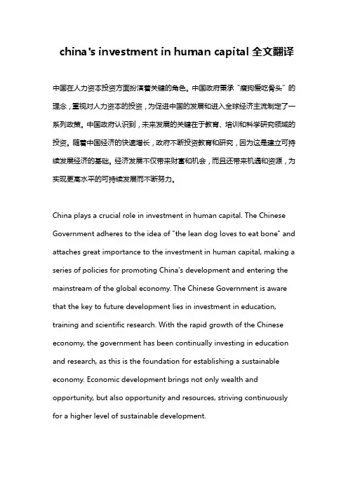
china's investment in human capital全文翻译中国在人力资本投资方面扮演着关键的角色。
中国政府秉承“瘦狗爱吃骨头”的理念,重视对人力资本的投资,为促进中国的发展和进入全球经济主流制定了一系列政策。
中国政府认识到,未来发展的关键在于教育、培训和科学研究领域的投资。
随着中国经济的快速增长,政府不断投资教育和研究,因为这是建立可持续发展经济的基础。
经济发展不仅带来财富和机会,而且还带来机遇和资源,为实现更高水平的可持续发展而不断努力。
China plays a crucial role in investment in human capital. The Chinese Government adheres to the idea of "the lean dog loves to eat bone" and attaches great importance to the investment in human capital, making a series of policies for promoting China's development and entering the mainstream of the global economy. The Chinese Government is aware that the key to future development lies in investment in education, training and scientific research. With the rapid growth of the Chinese economy, the government has been continually investing in education and research, as this is the foundation for establishing a sustainable economy. Economic development brings not only wealth and opportunity, but also opportunity and resources, striving continuously for a higher level of sustainable development.。
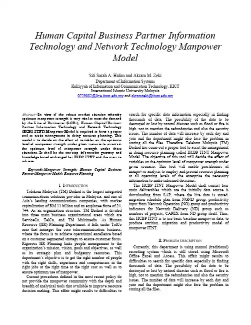
Human Capital Business Partner Information Technology and Network Technology ManpowerModelSiti Sarah A. Halim and Akram M. ZekiDepartment of Information SystemsKulliyyah of Information and Communication Technology, KICTInternational Islamic University Malaysia0729082@.my and akramzeki@.myAbstract—In view of the robust market situation whereby optimum manpower strength is very vital to meet the demand by the Line of Businesses (LOBs), Human Capital Business Partner Information Technology and Network Technology (HCBP ITNT) Manpower Model is required to have a proper tool to assist management in doing resource planning. This model is to decide on the effect of variables on the optimum level of manpower strength under given scenario to ascertain the optimum level of manpower strength under those situations. It shall be the one-stop information gateway and knowledge based exchanged for HCBP ITNT and the users to achieve.Keywords-Manpower Strength; Human Capital Business Partner;Manpower Model; Resource PlanningI.I NTRODUCTIONTelekom Malaysia (TM) Berhad is the largest integrated communications solutions provider in Malaysia, and one of Asia’s leading communications companies, with market capitalization of RM 11 billion and an employee force of 24, 744. As an organization structure, TM Berhad is divided into three main business organizational areas which are ServiceCo, TelCo, and TM Multimedia. As Human Resource (HR) Planning Department, it falls under TelCo area that manages the core telecommunication business, where the focus is to achieve operational excellence based on a customer segmented strategy to ensure customer focus. Rigorous HR Planning links people management to the organization’s mission, vision, goals and objectives, as well as its strategic plan and budgetary resources. This department’s objective is to get the right number of people with the right skills, experience and competencies in the right jobs at the right time at the right cost as well as to ensure optimum use of manpower.Current procedures defined in the most recent policy do not provide the manpower community with the depth and breadth of analytical tools that available to improve resource decision making. This affair might results to difficulties to search for specific data information especially in finding thousands of data. The possibility of the data to be destroyed or lost by natural disaster such as flood or fire is high, not to mention the redundancies and also the security issues. The number of data will increase by each day and year and the department might also face the problem in storing all the files. Therefore, Telekom Malaysia (TM) Berhad has come out a proper tool to assist the management in doing resource planning called HCBP ITNT Manpower Model. The objective of this tool will decide the effect of variables on the optimum level of manpower strength under given scenario. This tool will enable practitioners of manpower analysis to employ and present resource planning at all operating levels of the enterprise the necessary information to make informed decisions.The HCBP ITNT Manpower Model shall consist four main deliverables which are the initially data source is downloading from SAP, where the live data is stored, migration schedule plan from NGND group, productivity input from Network Operation (NO) group and productivity indicators for Network Delivery (ND) group such as numbers of projects, CAPEX from ND group itself. Thus, this HCBP ITNT is to use basic baseline manpower data, to produce attrition, migration and productivity model of manpower ITNT.II.P ROBLEM DESCRIPTIONCurrently, this department is using manual (traditional) recording system which is still stored using Microsoft Office Excel and Access. This affair might results to difficulties to search for specific data especially in finding thousands of data. The possibility of the data to be destroyed or lost by natural disaster such as flood or fire is high, not to mention the redundancies and also the security issues. The number of data will increase by each day and year and the department might also face the problem in storing all the files.Current procedures is defined in the most recent policy documents, while not necessarily incorrect, it does not provide the manpower community with the depth and breadth of analytical tools available to improve resource decision making. The tools developed using the manpower model outlined herein will enable practitioners of manpower analysis throughout the Network Technology to employ tools to present resource planning at all operating levels of the enterprise the necessary information to make informed decisions.III.S IGNIFICANT OF THE S YSTEMThe benefits of this models is to present overview and visibility of manpower numbers under the wing of CTIO namely Network Architecture & Technology (NAT), Network Delivery (ND), Service Fulfilment Centre (SFC), National Network Operation (NNO), Group Information Technology (GIT), Network Operation Centre (NOC) Project TOP, Operation & Programme Management, Technology & Innovation (T&I), TM R&D, Business Finance CTIO and Business Support, couple with input from migration planning, productivity indicators and attrition.Next, this model initially to establish online tool on manpower model under migration planning schedule, productivity and attrition input affecting the current manpower strength in IT&NT. It is able to assist in doing resource planning such as succession planning, job rotation, movement of position, promotion as well as to populate scenario on productivity, migration and attrition in `what-if-scenario’ environment.IV.R ELATED WORKSHuman resource planning has traditionally been used by organizations to ensure that the right person is in the right job at the right time [1]. Under past conditions of relative environmental certainty and stability, human resource planning focused on the short term and was dictated largely by line management concerns. Increasing environmental instability, demographic shifts, changes in technology, and heightened international competition are changing the need for and the nature of human resource planning in leading organizations. Planning is increasingly the product of the interaction between line management and planners. In addition, organizations are realizing that in order to adequately address human resource concerns, they must develop long-term as well as short-term solutions. As human resource planners involve themselves in more programs to serve the needs of the business, and even influence the direction of the business, they face new and increased responsibilities and challenges. [1]Workforce planning and scheduling entails anticipating supply availability and job requirements in order to have the right people, with the right skill, at the right time, in the right place, at the right cost [2]. The problem of matching future availability of employees with future job requirements is quite complex since HP has hundreds of thousands of employees in project delivery roles, with thousands of skills distributed in countries all over the world. The other challenge of matching future availability of employees with future job requirements is that supply and demand is uncertain. Finally, there are no clear costs when matching an employee to a job.V.SYSTEM ADAPTATIONFor HC BP ITNT Manpower Model, the features that would be included are Attrition Replacement of Job Position, Migration Staff Transfer that is subject to the business and operational needs in specific area, Productivity for Flexi Working Day or Working Hour and ‘Calculator’ to calculate, populate report and summary of chart of the models.VI.D EVELOPMENT APPROACHThe development approach for this system is incremental type which is the combination of linear and iterative frameworks [3]. A series of mini-waterfalls are performed, where all phases of the Waterfall development model are completed for a small part of the system, before proceeding to the next increment. This framework exists for exploiting knowledge gained in an early increment as later increments are developed. The moderate control is maintained over the life of the system through the use of written documentation and the formal review and approval/signoff by the user and information technology management at designated major milestones. It also helps to mitigate integration and architectural risks earlier in the system.Moreover, this framework allows delivery of a series of implementations that are gradually more complete and can go into production more quickly as incremental releases. It requires highly interactive applications where the data for the system already exists (completely or in part), and the system largely comprises analysis or reporting of the data. Stakeholders can be given concrete evidence of the system status throughout the life cycle and gradual implementation provides the ability to monitor the effect of incremental changes, isolate issues and make adjustments before the organization is negatively impacted.Basically, this model shall consist of the following main deliverables:1)Initially data source is downloading from SAP.2)Migration schedule plan from NGND Group3)Productivity input from Network Operation (NO) Group.4)Productivity indicators for Network Delivery (ND) group such as numbers of projects, capex from ND Group itself etc.Thus, to use basic baseline manpower data, to produce attrition, migration and productivity model for manpower ITNT.For the target user of HC BP ITNT Manpower Model system is for the Network Development Department in HR Planning. People in this department would have control over the system which is the data is latest upon user update.VII.REQUIREMENT SPECIFICATIONFor this model, there have three main features which are Attrition model, Migration model and Productivity Model. In Attrition model, the division will confirm the replacement requirements including new intake, acting and reassignment in monthly meeting. Then, the Human Capital Business Partner (HCBP) will be verify using this manpower model and the replacement plan are agreed which is endorsed by Vice President (VP). Next, HCBP submit to Group Human Capital Management (GHCM) for temporary post ID creation and instruct Human Capital Shared Service Organization (HCSSO) to move body to temporary post. Then, the HCSSO will inform HCBP if post ID is available to execute for recruitment, transfer, acting, or redeployment. In Migration model, the transfer is subject to the business and operational needs in specific area. The job scope and competency required are well defined. The transfer could be prioritized within state with exception of Wilayah Persekutuan Labuan branch and transfer body and position (lock stock and barrel) is allowed. All transfer must obtained Human Capital Board of Director approval via HCBP and based on business call.Lastly in Productivity model, the working hours are not more than 39.5 hours per week as per Article 29.2 Collective Agreement 8. Flexi rest days are on Saturday and Sunday or Thursday and Friday or Friday and Saturday (for Kelantan, Kedah, and Terengganu). The flexible lunch break is one hour. Number of management to decide on the needs of flexi rest days and flexi working hours schedule is based on operational needs. The schedule is going to be published to staff at least one month before the effective date.The overtime policy is apply as usual for outside working hours and the frequency of flexi working day and hour is up to business requirements. This flexi rotation is done for every four weeks. Figure 1 below shows the useFigure 1. Use Case Diagramcase diagram and Table 1 shows the partial list of HCBP ITNT Manpower Model use case.TABLE 1. Partial List of HCBP ITNT Manpower Model Use CaseUse-Case name Use-Case Description Participating Actors andRolesDownload raw data from SAP This use case describes the event of a NGND Group/Staffrequesting and downloading the raw data from SAP to bereviewed.NGND Group/Staff (primarybusiness)Generate migration plan table This use case describes the event of a NGND Group/Staffgenerates the migration table from SAP’s raw data.NGND Group/Staff (primarybusiness)Get productivity input This use case describes the event of a NO Group/Staffrequesting and downloading the raw data from SAP to bethe productivity input for Flexi Working Day/WorkingHour.NO Group/Staff (externalreceiver)Extract data into This use case describes the event of a NGND Group/Staffrequesting and downloading the raw data from SAP to besort, query and generate information from the AttritionModel, Migration Model and Productivity Model. NGND Group/Staff (primary business)Check variables This use case describes the event of a NGND Group/Staffchecks the variables from generated migration table. (eg.Exchange location, migration date, no of docket, workstream, replacement rules, etc.) NGND Group/Staff (primary business)Verify output This use case describes the event of a NGND Group/Staffverifies the variables from generated migration table (eg.Exchange location, migration date, no of docket, workstream, replacement rules, etc.) whether to replace, remain,abolish post or redeploy post. NGND Group/Staff (primary business)This use case glossary explains the relationship between the event and the use case that participate by actors. These actors can be defining as roles.Figure 2 shows that the flows diagram of HCBP ITNT Manpower Model. Initially, the source of data is downloading from SAP where the live data is stored.Figure 2. Data Flow DiagramThe NGND group will generate the migration schedule plan into the system. While the NO Group generates the productivity input. The ND groups then checks the variables, delivers productivity indicators and extract all the data from the system. The rules and guidelines are applied into attrition, migration and productivity model. Then, the important group, which is ITNT group, would maintain the system need to update the entire data source into the system.VIII.D ATABASE D ESIGNDatabase design is the process of producing a detailed data model of a database. This logical data model containsall the needed logical and physical design choices and physical storage parameters needed to generate a design in a Data Definition Language, which can then be used to create a database. A fully attributed data model contains detailed attributes for each entity.The term database design can be used to describe many different parts of the design of an overall database system. Principally, and most correctly, it can be thought of as the logical design of the base data structures used to store the data. In the relational model these are the tables and views. In an object database the entities and relationships map directly to object classes and named relationships. However, the term database design could also be used to apply to the overall process of designing, not just the base data structures, but also the forms and queries used as partof the overall database application within the database management system (DBMS).Database designs also include ER (Entity-relationship model) diagrams. Figure 3 shows the entity relationship diagram of HCBP ITNT Manpower Model.Fi gure 3. Entity Relationship of HCBP ITNT ManpowerModel.IX.C ONCLUSIONThe purpose of manpower planning is to ensure that the right people are in the right place at the right time, it must be linked with the plans of the total organization. Traditionally, there has been a weak one way linkage between business planning and human resource planning. Business plans, where they exist, have defined human resource needs, thereby making human resource planning a reactive exercise.Organizations of the future are likely to be in a state of continuous change and uncertainty. Therefore, in view of the robust market situation whereby optimum manpower strength is very vital to meet the demand by the (line of Businesses (LOBs), Human Capital Business Partner IT & NT (HC BP ITNT) is required to have a proper tool to assist management to assist in doing resource planning such as succession planning, job rotation, movement of position, promotion etc. This model is to decide on the effect of variables on the optimum level of manpower strength under given scenario to ascertain the optimum level of manpower strength under those situations. It shall be the one-stop information gateway and knowledge based exchange for HC BP IT&NT and the users to achieve.As organizations change more quickly, so will the knowledge, skills, and behaviors needed from employees.This means that people working in organizations will be asked continually to adjust to new circumstances. Assessingand facilitating peoples' capacity for change are two activities that psychologists are likely to be called on to do,yet there is very little research available to consult for guidance. Whereas organizations are seeking changes from employees, employees will be demanding that organizations change to meet the needs of the increasingly diverse work force. Research designed to help us understand how organizations can establish and maintain employee flexibility and adaptability is likely to make an important contribution.REFERENCES[1]Susan E. Jackson and Randall S.Schuler (1990). Human resourceplanning - challengers for industrial/organizational psychologists.45(2), pp 223-239.[2]Cipriano A. Santos, Alex Zhang, Maria Teresa Gonzalez, and ShelenJain (2009). Workforce planning and scheduling for HP IT servicebusiness.[3]Pressman, R. S. (2010). Software engineering: a practitioner’sapproach (7th ed.). New York: McGraw-Hill.[4]User Requirement Specification for HCBP ITNT Manpower Model,Version 1.0, June 2010.[5]User Requirement Specification for HCBP ITNT Manpower Model,Version 1.1, January 2011.[6]John T. Marchewka (2010). Information technology projectmanagement (3rd ed.). John Wiley.[7]Kostiuk P.F. (1987). Naval planning manpower and logistics division;the navy manpower-requirements system, CRM 87-114 [Accessed 23August 2011].[8]EUROCONTROL,1998. A system view of manpower planning andmanagement [online]. Available from: http://www.eurocontrol.int/humanfactors/gallery/content/public/docs/DELIVERABLES/M25-HRS-MSP-003-REP-025withsig.pdf[Accessed 23 August 2011].[9]EUROCONTROL,1996.Report on Issues in ATCO manpowerplanning [online]. Available from:http://www.eurocontrol.int/humanfactors/public/site_preferences/display_library_list_public.html [Accessed 11 January 2011].[10]Connolly, T.&Begg,C.(2005).Database systems;a practical approachto design, implementation and management. 5th Ed. England:AddisonWesley, Pearson Education.。
A Puzzle and Some AnswersRuth JudsonFederal Reserve BoardJune 1995In this paper, I develop a new measure of human capital stock that has two advantages over previous measures. First, it allows for the fact that the cost of education varies across time, countries, and levels. Second, the unit of measurement is dollars, which allows comparison of human capital stocks with other macroeconomic variables, including national income (GDP) and physical capital stocks. Using cross-country panel regression analysis, I find that human capital accumulation accounts for a relatively small (about ten percent) of per-capita GDP growth. I further find that, unlike physical capital, the stock of human capital as a share of GDP increases with GDP.on the puzzle of why the human capital coefficient is often lower than theory would predict, and whether such estimates are believable. In order to do this, I develop a new measure of human capital stocks that has two advantages over previous measures. First, it allows for the fact that the cost of education varies across time, countries, and levels. Second, the unit of measurement is dollars, which allows comparison of human capital stocks with other macroeconomic variables, including national income (GDP) and physical capital stocks. Using cross-country panel regression analysis, I find that human capital accumulation accounts for a relatively small (about ten percent) of per-capita GDP growth. I further find that, unlike physical capital, the stock of human capital as a share of GDP increases with GDP.A Puzzle and Some AnswersIndividuals and governments invest vast quantities of resources in education, and there is substantial evidence that it is a worthwhile investment: individuals who are more educated earn higher wages, richer countries have higher levels of literacy and educational attainment, and the countries that experience rapid economic growth are often the ones that have invested heavily in education. Education, or the human capital it creates, is a key input in new macroeconomic models, including those of Lucas (1988), Romer (1990), Jovanovic, Lach, and Lavy (1992), and Azariadis and Drazen (1990).In the past five years, new cross-country macroeconomic datasets have been assembled by Heston and Summers (1992), the World Bank, the International Monetary Fund, and others. These datasets include measurements of key macroeconomic variables for as many as 138 countries and 41 years. They allow economists to analyze economic growth and development with data from a wide sample of countries, circumstances, and stages of development.Since education is supposed to be important, we might expect measures of education to enter significantly and with large coefficients in regressions that analyze growth. There are three basic types of growth regression that researchers estimate; only one yields any significant role for human capital. The first type of regression is a reduced form regression. In these regressions, average GDP growth rates are regressed on initial conditions and other level and change variables that are expected to influence growth. The second type of regression is based on the growth decomposition of the Cobb-Douglas production function. In these regressions, GDP growth is regressed on growth rates of factor inputs. Estimation of these two types of regressions has typically yielded implausibly low,1statistically insignificant, or negative coefficients on human capital variables. The last type of regression is based on an extension of the Solow (1957) model's predictions about steady-state growth. It is this type of estimation that yields the one exception: a high, positive, and statistically significant coefficient for human capital. Mankiw, Romer, and Weil (1992) add human capital to the Cobb-Douglas production function used by Solow and find that estimation of the steady-state equation yields a coefficient around 0.3 for human capital, implying a share in production and an elasticity with respect to growth of nearly one third.Table 1 displays the results of estimation of the human capital coefficient from various studies. The first column identifies the study; the second through fourth columns identify the estimation method, model, and measure of human capital (HK) used. The coefficient estimates are not directly comparable with each other because the human capital variable is not always a growth rate. Mankiw, Romer, and Weil (1992) use secondary school enrollment as a proxy for human capital accumulation; they claim that secondary enrollment is collinear with human capital accumulation, w h i c h i s a l l t h e y n e e d i n t h e i r m o d e l.2Table 1: Summary of Cross-Country Regression ResultsAuthor Model Human Capital(HK)VariableTechnique Coefficient TMankiw, Romer & Weil 1992Augmented Solow,Steady stateSecondaryenrollmentCross-sectionOLS0.289.3Barro and Lee 1992Reduced form Log of Barro-Lee HKCross-sectionOLS0.057 3.0Barro and Lee 1992Reduced form Log of Barro-Lee HKPooled panel0.021 5.2Romer 1990Reduced form Literacy rate,change Cross-sectioninstrumentalvariables0.204 2.3WDR 1991Augmented Solow,production function WDR HK,changePooled panel,annual dataEd<3 yrs: 0.09Ed>3 yrs: 0.042.62.0Benhabib-Spiegel, 1992Augmented Solow,production functionKyriacou HK,changeCross-section-0.021 1.4Lau et al., 1991Augmented Solow,production functionWDR HK, logdifferencePooled panel,annual0.016 1.6Judson 1993Augmented Solow,production function Judson HK,growth ratePanel GLS0.098 4.3World Development Report (1991) and Benhabib and Spiegel (1992) also use absolute changes inaverage years of education of the labor force rather than percentage changes. Romer (1990) considers literacy a proxy for human capital stock and uses the change in the literacy rate. Barro and Lee (1992) use the log level of their measure of average education of the labor force. Finally, Lau, Jamison and Louat (1991) use the log difference of the World Development Report's (1991) measure of average years of education of the labor force, which is approximately equal to the percentage growth rate. This is the only measure that is comparable to the growth rate that I use; I obtain a3coefficient of 0.098, more than five times that obtained by Lau, Jamison, and Louat (1991) but only a third as large as that obtained by Mankiw, Romer, and Weil (1992).Three questions emerge: first, which estimate of the parameter for human capital in a Cobb-Douglas production function is correct econometrically? Second, does the coefficient make sense in the context of both micro evidence about returns to education and the Cobb-Douglas production function? Third, what are the implications for human capital investment and our understanding of economic growth if the lower coefficient is right?In this chapter, I first outline the extended Solow model proposed by Mankiw, Romer, and Weil (1992). I use the same production function as they do to link the relative returns to human and physical capital, the relative stocks of human and physical capital in the economy, and their relative coefficients in the regression equation derived from the same model. I then review the evidence on returns to physical and human capital investment across countries and time. Next, I develop a new human capital series that measures the stock of human capital in value rather than in person-years. This measure of human capital eases comparison of the stock of human capital with that of physical capital over time and across countries. Finally, I review and test the specifications of the extended Solow model that have produced the macroeconomic parameter estimates.Using the new measure of human capital stock and the production function specification, I find a robustly positive human capital coefficient that is two to three times larger than comparable figures found in earlier studies but still well below the estimate of 0.3 of Mankiw, Romer, and Weil (1992). Further, I find that a low value for the share of human capital in the growth decomposition is plausible both econometrically and in the context of the Cobb-Douglas form of the production function, and that the relationship between human and physical capital stocks and returns and their regression coefficients predicted by the production function in Mankiw, Romer, and Weil's (1992)4extended Solow model holds approximately. Human capital thus belongs in the production function and is still a high-return input, but its role is not as large as that of physical capital.However, I also find that the path of human capital accumulation as wealth increases is distinctly different from that of physical capital: the human capital to output ratio is increasing in output but the physical capital to output ratio shows no trend. This is not explained or predicted by any of the new growth models that I am aware of. However, the Solow model does not predict these patterns either. Measuring human capital as I do also allows me to examine some of the predictions about human capital accumulation and growth that are implied by newer models of growth. I find that none of the predictions of the new growth theory about the relationships between levels and growth rates of income and human capital hold. In sum, while the Cobb-Douglas form of production in the augmented Solow model provides a reasonable description of growth, it must be considered a starting point rather than an endpoint in our thinking about the role of human capital in growth and development.In Section 1 I derive the relationship between human and physical capital levels, returns, and regression coefficients that is implied by the extended Solow growth model with a Cobb-Douglas production function. In Sections 2, 3, and 4 I discuss the data available for the three ratios that form this relation. First, in Section 2, I review the evidence on returns to human and physical capital. Second, in Section 3, I develop a new human capital series that measures the value of education embodied in the labor force at a particular time. Third, in Section 4 I estimate the parameters of the Cobb-Douglas production function with a cross-country panel regression. I also calculate productivity residuals and review other regression estimates of the production function parameters. In Section 5, I conclude and discuss the implications for human capital accumulation. In Section 6 I return to the properties of the data and compare them to the predictions of several new growth models.56 I. The Extended Solow Model and the Human Capital CoefficientA. The Solow Growth DecompositionIn the original Solow (1957) growth decomposition, technical progress is neutral so that production takes the form:(1) If the production function is Cobb-Douglas in physical capital and labor, then(2) Taking time derivatives of the production function and dividing through by Y yields:(3) In per worker growth rate terms we have:(4) In order to measure the productivity residual, Solow calculated the input share for physical capital for each year. He assumed constant returns to scale and complete classification of inputs as either physical capital or labor so that the shares would sum to one. He then calculated productivity residuals using this equation and data on output per man-hour and physical capital per man-hour. Solow estimated a separate physical capital share variable for each year. He found that physical capital's share in income varied from a low of 0.312 to a high of 0.397.New cross-country datasets permit similar analysis across a large sample of countries. However, the data available in these datasets are not nearly as rich as those available for the U.S.Constant returns are imposed by setting equal to 1--.17 In particular, factor shares are not available, but growth rates of inputs are. Dropping the constant-returns-to scale assumption, imposing constancy of factor shares, and adding an error term yields the regression form of the Solow growth decomposition:(5) Cross-country regressions with panel and cross-section data yield coefficient estimates close to those calculated by Solow; these will be discussed in Section IV.B. The Extended Solow Model with Human CapitalMankiw, Romer and Weil (1992) propose an extension of the Solow model in which production is Cobb-Douglas in three inputs: labor (L), physical capital (K), and human capital (H):1(6) As with the original Solow model, taking time derivatives, imposing constant returns to scale, and adding an error term yields an equation for the growth of output in terms of growth of labor, physical capital, and human capital:(7)Assuming that inputs are paid their marginal products, this model allows us to write an equation relating rates of return, levels, and coefficients for pairs of inputs. First, note that if returns8 are equal to marginal products, then(8) Taking the ratio of marginal products gives(9) which is the relationship I will examine. I calculate the three ratios in this equation and show that, on average, they satisfy this equation. The ratio of returns is discussed in Section 2, the ratio of the stock of human capital to physical capital is calculated in Section 3, and the ratio of the coefficients of the production function is estimated in Section 4.II. Returns to Human and Physical CapitalA. Returns to Human Capital in the Form of EducationProponents of investment in education argue that education is a good investment because it yields a high return, usually much higher than that of physical capital. Indeed, the rates of return calculated and compiled by Psacharopoulos (1993, 1985) are impressively high. Table 2 displays rates of return to education calculated and assembled by Psacharopoulos (1993). For each region, the average includes the most recent observation for each country for which data are available. Private rates of return are higher than social rates of return because private returns exclude the publicAll returns to education are assumed to be captured by the individual's wage; social 2benefits to adding to the stock of educated people are not measured in the calculation of either private or social rates of return.9Table 2: Rates of Return to Education, Various Levels, By RegionRegionSocial Private PrimarySecon-dary Higher Primary Secon-dary Higher Sub-Saharan Africa24.318.211.241.326.627.8Asia (non-OECD)19.913.311.739.018.919.9Europe/M.East/N.Africa15.511.210.617.415.921.7Latin America/Caribbean17.912.812.326.216.819.7OECD14.410.28.721.712.412.3World 18.413.110.929.118.120.3Source: Psacharopoulos (1993), p. 7.component of the costs of education. As with physical capital returns, I construct five-year 2averages of the return to education data, which are available quite sporadically. Figure 1, Figure 2,and Figure 3 display private rates of return to primary, secondary, and higher education against GDP.Rates of return to all levels of education fall as GDP rises.These rates of return were calculated either by the earnings function method due to Mincer (1974) or by what Psacharopoulos (1993) calls the full method. In the full method, the return is the discount rate that equates the costs of education, including foregone wages and other costs, and the benefits of education in the form of increased wages. Social rates of return include in the costs of education both foregone income and the full cost of education, including that borne by thegovernment; private returns include only foregone income and private educational expenses in the cost of education. Since the private costs of education are often lower than the social costs, private rates of return to education are usually higher than social rates of return.The full method is a compromise between the earnings function method due to Mincer (1974), which requires less data but is less flexible, and the net present value method, which is better but requires comprehensive earnings and education data on many individuals. The full method has two prominent drawbacks. First, it is very difficult to measure the ability of the students, which is clearly an important input (See, e.g., Griliches (1977)). Second, it is difficult to calculate foregone earnings for children in general and for the very uneducated in countries where primary education is close to universal. In fact, it is nearly impossible to obtain the relevant wage data for children from cross-country sources because countries are unwilling to admit that they have child labor, which they would implicitly do by providing such data. These problems are common, however, to many measures of returns to education. In the full method, researchers can adjust for the fact that foregone income for children might be less than that for adults by assuming that children only forego income for part of their time in school. However, Psacharopoulos (1993) notes that relatively few studies do this.The full method is the method preferred by Psacharopoulos (1993). However, for some countries, only rate of return data calculated by the earnings function method are available; in this case, Psacharopoulos reports them. In the earnings function method, the log of wages is regressed on a constant, years of schooling, years of experience, years of experience squared, and other relevant variables. In such a regression, the private rate of return to a year of education comes from the coefficient on years of education. This method has the same drawbacks as the full method; in addition, as Psacharopoulos and Layard (1979) and Psacharopoulos and Ng (1992) have pointed out, it requires the assumption that earnings are the same at all times for a given level of education.10I am grateful to Elaine Buckberg for providing these data.311Finally, both methods of estimating rates of return to education could be modified to allow for different rates of return to different types of education or different specializations, but data at this level of disaggregation are not available across many countries.B. Returns to Physical CapitalData on returns to physical capital that are comparable across a broad sample of countries are scarce, but they do exist. Some data are available on rates of return to public investment projects funded by the World Bank, but these data are confidential, spotty, and refer only to particular projects. In addition, the World Bank is not a typical investor. An alternative source of data is the rates of return for United States direct investment abroad, which are compiled by the Bureau of Economic Analysis. Although these data also focus on a small subsample of investment in each 3country, the measurements are consistent with each other and offer a means of comparing returns to physical capital across a broad sample of countries and time periods. In addition, they represent the returns to physical capital that can be obtained by private investors who have many investment options. I calculate returns to physical capital from the BEA data. For a given country and time period, returns are calculated as earnings divided by total investment outstanding. The BEA data are provided on an annual basis. In order to make them comparable to the rest of my data, I construct five-year averages of the returns.Table 3: GDP Quintile, Region, and Time Averages of Returns to Capital and Human CapitalI. Quintile averages sorted by GDPC, per-capita GDP.Quintile GDPC KRET PPRET SPRET HPRET159313.325.418.624.12118911.430.920.825.53214912.632.920.117.84417912.919.714.118.55983112.821.612.312.8 II.Quintile averages sorted by KRET, returns to physical capital.Quintile GDPC KRET PPRET SPRET HPRET15925 5.520.212.715.1264479.325.217.417.43666012.429.412.211.94704915.512.510.915.85707022.3 .18.525.2 III. Sorting by regionRegion GDPC KRET PPRET SPRET HPRETOECD861512.220.512.312.3LACAR352911.623.815.620.0MENA419819.512.717.821.8ASIA243815.926.815.816.7AFRICA128714.036.125.725.6 IV. Sorting by periodPeriod GDPC KRET PPRET SPRET HPRET61-65243610.721.215.213.566-7028589.326.917.517.071-75346811.525.213.417.676-80394814.519.714.417.881-85415113.044.124.325.286-90464216.723.616.217.4 GDPC: Per-capita GDP, in 1985 PPP dollars from Heston-Summers 1992. KRET:Rate of return to capital on U.S. Foreign Direct Investment, from BEA. PPRET,SPRET, HPRET: Private return to primary, secondary, and higher education, fromPsacharopoulos (1993).12Table 3 provides descriptive statistics about returns to physical capital. In the first panel, the data are grouped into quintiles according to per-capita GDP. Thus, the first row displays group averages for the poorest twenty percent of the sample and the fifth row displays group averages for the richest quintile of the sample. We see that rates of return to physical capital do not vary systematically with GDP. However, returns to human capital decline as GDP increases. In the second panel, with quintile averages sorted by returns to physical capital (KRET), we see that per-13capita GDP increases moderately with returns to physical capital but the other variables do not move with KRET in a systematic way. In the third and fourth panels, averages over regions and time periods, the same general patterns and correlations are discernible: GDP increases over time and is negatively correlated with returns to human capital; returns to physical capital increase weakly over time.C. Stocks of Physical CapitalI use a physical capital stock dataset that was originally created for the 1991 World Development Report and subsequently updated by Nehru (1992). This series measures total capital stock using the perpetual inventory method and an initial capital stock value of zero. The measurements are in 1987 national currency units. In order to compare physical capital stock to GDP and human capital stocks, I use the IMF's real GDP figures. Since the IMF reports real GDP in 1985 units, I inflate the GDP series using either the IMF's GDP deflator where available and the consumer price index from the IMF otherwise.Figure 4 to Figure 7 illustrate the relationships between returns to physical capital and the capital-labor ratio, capital per head, the ratio of human capital to physical capital, and GDP. There is little pattern to returns to physical capital: they are weakly positively correlated with the capital-output ratio and capital per capita; they are not correlated with GDP. Returns to physical capital are weakly negatively correlated with the ratio of human to physical capital. On average, rates of return to physical capital are lower than those for human capital. Across available observations, the mean ratio of physical capital returns to private human capital returns is 0.52 for primary education, 0.65 for secondary education, 0.68 for higher education, and 0.47 overall.14III. A New Human Capital SeriesI develop a new human capital series that estimates the value, in 1985 PPP dollars, of a country's human capital stock. Such a series has two advantages over existing measures and proxies for human capital stock. Many studies do not use direct measures of human capital; rather, they use proxies such as literacy (e.g., Benhabib and Spiegel (1993), Romer (1990)) or enrollment rates (e.g., Mankiw, Romer, and Weil (1992)). The proxies give an idea of how much human capital a country has, but any power they have depends on the assumption that the proxy is collinear with the country's whole human capital stock. More recent studies use series that measure human capital stock as average years of education of the labor force, as by World Development Report (1991) and Barro and Lee (1992). These series do not account for the fact that the relative cost of a year of primary education compared to that of higher education is not one and is not constant across countries. Nor do they account for the fact that the resources devoted to a year of primary, secondary, or higher education vary considerably across countries and time. In addition, person-years of education are difficult to compare to capital stocks, GDP, or other macroeconomic variables. This series corrects both problems.My human capital series builds on those of Barro and Lee (1992) and Nehru et al. (1993), which measure the average educational attainment of the labor force in years of education. My innovation is to calculate the cost of education and to then weight primary, secondary, and higher education stocks according to their costs. This improvement is analogous to measuring physical capital by the cost of types of buildings and machines rather than just the number of them. It allows comparison of human capital stocks with physical capital stocks and GDP. In addition, growth rates of my series incorporate the changes as countries shift from expanding primary education, which is relatively inexpensive, into secondary and higher education, which tends to be more expensive.15After discussing the construction of the series and presenting some descriptive statistics, I demonstrate that human capital accumulation behaves rather differently from that of physical capital. Finally, I use the series to form the ratio of physical to human capital, which gives the second ratio in Equation (9).A. OverviewMy human capital series combines data from three sources. I begin with Barro and Lee (1992) and Nehru et al. (1993) data on the average educational attainment of the labor force by level. Second, I use UNESCO data on school enrollments by level and education spending by level to obtain weights for the education stock at each level. I calculate per-pupil spending at each level of education for each country in each of the six five-year periods between 1960 and 1990. I use these spending figures to weight primary, secondary, and higher educational attainment as given by Barro and Lee (1992) and Nehru et al. (1993). This gives me a value for a country's total educational stock in nominal national currency units. Third, I convert these figures to 1985 prices using the UNESCO series on educational spending as a share of GDP and Heston-Summers GDP data. I use five-year intervals because most of the underlying data series are only available at five-year intervals anyway. Where more than one observation is available for a particular period, I use the average over available observations.B. Sources of DataI base my calculations on estimates of the average educational attainment of the labor force developed by Barro and Lee (1992) and Nehru et al. (1993). Both series consist of measurements of average primary, secondary, higher, and total educational attainment for a panel of about 8016Research on educational inputs in the United States indicates that current4expenditures are much more highly correlated with school quality than capital or totalexpenditures. See, e.g. Schmidt (1993).17countries and the six five-year periods between 1960 and 1990. The two series differ in coverage,but are closely correlated (=0.75). They arrive at their estimates rather differently, however. Barro and Lee (1992) use census data as their starting point and augment it with other information about school enrollment and completion. Nehru et al. (1993), in a refinement of Jamison, Lau, and Louat (1991), use enrollment data as a base. Both methods require substantial simplifying assumptions and extrapolation. Barro and Lee measure the educational attainment of the labor force aged 25-64;Nehru et al. (1993) include all members of the labor force aged 15-64. Thus, Nehru et al.'s (1993)figures are more likely to capture more recent expansion of education in less developed countries.In addition, Nehru et al.'s (1993) dataset provides more observations. Thus, I use Nehru et al.'s (1993) series for the results reported here. However, the results do not change much when Barro and Lee's (1992) series is used.To estimate the relative value of a year of education at each level, I use data from UNESCO and Heston-Summers (1992). UNESCO reports data on total, current, and capital spending on education by level in national currency units; it also reports total current spending as a share of GDP.I use current spending as the measure of spending for three reasons. First, it is available for a much larger sample of countries and periods than are capital and total spending. Second, it is a smoother measure of educational inputs. Third, it measures the most important educational inputs at least as accurately as total spending. UNESCO reports enrollment by sex, age, and level. I use total 4enrollment at each level for both sexes. I choose this measure for two reasons. First, it is more widely available. Second, it does not make sense to ignore older students since they too are accumulating human capital and using educational inputs.。
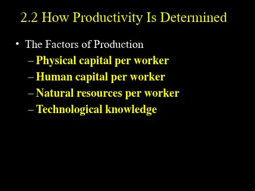
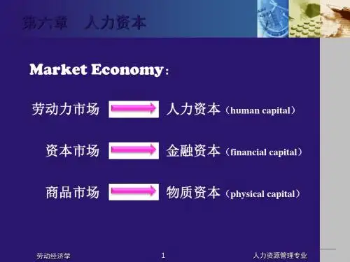
Human capital refers to the skills,knowledge,and experience that individuals possess,which contribute to the productivity and economic growth of a society.It is a critical component of a nations wealth and is often considered as important as physical capital,such as machinery and infrastructure.The Concept of Human CapitalThe concept of human capital was first introduced by economists to highlight the value of education and training in enhancing an individuals ability to contribute to the economy.It is based on the idea that investing in peoples skills and knowledge can yield returns, much like investing in physical assets.Investment in Human CapitalInvestment in human capital takes various forms,including formal education,vocational training,health care,and even early childhood development programs.These investments are believed to increase an individuals earning potential,job satisfaction,and overall quality of life.Education as a Key ComponentEducation is a fundamental aspect of human capital development.A welleducated workforce is more likely to be innovative,adaptable,and capable of driving technological cation not only imparts knowledge but also fosters critical thinking and problemsolving skills.Health and Human CapitalGood health is another essential element of human capital.Healthy individuals are more productive and can contribute more effectively to the economy.Investments in public health,such as immunization programs and access to healthcare services,are therefore crucial for building a robust human capital base.The Role of GovernmentGovernments play a pivotal role in developing human capital by creating policies and programs that support education,health,and social welfare.This includes funding public schools,regulating labor markets,and ensuring access to healthcare.Challenges in Human Capital DevelopmentDespite its importance,human capital development faces several challenges.These include disparities in access to quality education and healthcare,gender and income inequality,and the need to keep pace with rapidly changing technological landscapes. The Impact of Human Capital on Economic GrowthA strong human capital base is linked to higher economic growth rates.Countries with a highly skilled and educated population tend to have lower unemployment rates,higher innovation,and greater competitiveness in the global market.ConclusionIn conclusion,human capital is a vital resource for any economy.It is the sum of the skills,knowledge,and health of a population that can be leveraged for economic advancement.By investing in human capital,societies can ensure sustainable growth and improve the wellbeing of their citizens.。
资本换取了你的生命作文英文回答:The concept of "capital over life" is a complex and multifaceted one, with implications that extend beyond the realm of economics. Within the capitalist system, the pursuit of profit and accumulation often takes precedence over the well-being and lives of individuals. This prioritization of capital over human life is evident in various aspects of society, from the exploitation of workers in sweatshops to the environmental degradation caused by unregulated industrial activities.The commodification of life under capitalism reduces individuals to mere cogs in the economic machine, their value determined by their ability to generate profit. This process of dehumanization is reflected in the language we use to describe workers as "human capital" or "resources." The focus on maximizing productivity and efficiency often comes at the expense of workers' health, safety, and well-being.Furthermore, the pursuit of capital accumulation often leads to the accumulation of wealth and power in the hands of a few, while the majority of people are left struggling to meet their basic needs. This inequality is not simply a matter of resource distribution but also a reflection of the systemic oppression and exploitation inherent in capitalism.The prioritization of capital over life has profound implications for the sustainability of our planet. The relentless pursuit of economic growth has led to the overconsumption of natural resources and the destruction of ecosystems. The consequences of environmental degradation are already being felt in the form of climate change, air and water pollution, and loss of biodiversity.Addressing the issue of "capital over life" requires a fundamental re-evaluation of our values and priorities. It necessitates a shift away from a system that prioritizes profit accumulation and towards one that centers on humanwell-being and the preservation of the natural environment.中文回答:资本换取生命,这是一个复杂且多方面的概念,其含义超出了经济范畴。
资本家和企业家的作文800字英文回答:As a capitalist, my main goal is to accumulate wealth and make a profit. I invest my money in various businesses and industries, hoping to generate a return on my investment. I take risks and make strategic decisions based on market trends and opportunities. I am driven by the desire to maximize my profits and grow my wealth.For example, I might invest in a tech startup that has the potential to disrupt the market and generate high returns. I provide the necessary capital and resources for the startup to grow and expand. In return, I expect a share of the company's profits or a significant return on my investment.I am also aware of the risks involved in investing. Sometimes, I may experience losses or face challenges in the market. However, I am willing to take these risksbecause I believe in the potential for high returns. I constantly analyze market conditions and adapt my investment strategies accordingly.On the other hand, as an entrepreneur, my focus is on creating and running my own business. I am driven by passion and the desire to bring my ideas to life. I take on the responsibility of managing the business, making strategic decisions, and ensuring its success.For instance, I might start a small bakery because I have a passion for baking and want to share my delicious treats with others. I invest my time, energy, and resources into setting up the bakery, hiring staff, and marketing my products. I take pride in the quality of my baked goods and strive to provide excellent customer service.As an entrepreneur, I also face challenges and risks. I may encounter competition, financial difficulties, or other obstacles along the way. However, I am determined to overcome these challenges and make my business thrive. I am constantly innovating, adapting to market trends, andfinding ways to differentiate my products or services.In conclusion, both capitalists and entrepreneurs play important roles in the economy. While capitalists focus on accumulating wealth and making profits through investments, entrepreneurs are driven by passion and the desire tocreate and run their own businesses. Both face risks and challenges but are motivated by the potential for success and growth.中文回答:作为一个资本家,我的主要目标是积累财富和获得利润。
china's investment in human capital总结随着中国经济的不断发展和全球化的趋势,中国对人力资本的投资越来越受到重视。
以下是中国对人力资本投资的总结:
1. 教育:中国政府在教育方面的投资一直很大,尤其是在基础教育、高等教育和职业教育方面。
中国政府还鼓励民间资本进入教育领域。
近年来,中国高等教育的质量和国际排名也有了很大的提高。
2. 健康:中国政府也在健康领域投资,包括基础医疗设施、医疗保险和公共卫生项目。
中国政府还鼓励私人医疗机构的发展。
这些投资都有助于提高中国人民的健康水平和生活质量。
3. 科技:中国政府在科技领域的投资也很大,尤其是在高科技和创新领域。
中国政府还鼓励企业进行创新和研发工作。
这些投资有助于提高中国的技术水平和竞争力。
总的来说,中国对人力资本的投资是全面、持续和长期的。
这些投资有助于提高中国人民的教育水平、健康水平和技术水平,促进中国经济的发展和全球竞争力的提升。
- 1 -。
How to Enhance ROI of Human Capital Through TrainingPresenter:Raymond Lo, Senior ManagerDeloitte Human Capital Advisory Services Limited 21 June 2002How to Enhance ROI of Human Capital Through TrainingAn OverviewWhy Care about ROI of Human Capital? Enhancing ROI of Human Capital Training Initiatives Measuring Training Effectiveness Q&AHow to Enhance ROI of Human Capital Through TrainingWhy Care about ROI on Human Capital?What is Human Capital?Human Capital (“HC”): is an intangible asset of a company inspires ideas that ignite values financial analysts pay higher attention on HC leverages on measuring the company’s worth¾ E.g. General Electric, Nokia, Microsoft¾ Intelligence and values of employees can generate multi-fold of revenues and are reflected on stock pricesHow to Enhance ROI of Human Capital Through TrainingWhy Care about ROI on Human Capital?Human Capital ComponentsTechnical Know-How &EducationIdeas & InsightsLessons LearntCreativityHuman CapitalKnowledge ManagementUndocumented MethodologiesSkills & KnowledgeMarket ResearchHow to Enhance ROI of Human Capital Through TrainingWhy Care about ROI on Human Capital?Corporate Investment on Human CapitalHuman CapitalCustomer AssetsIntellectual AssetsUS$1.0 – 3.1 TrillionIntangible AssetsBusiness RelationshipUS$10.4 TrillionOrgan’l AssetsTangible AssetsUS$2.0 TrillionMarket ValuesUS$12.4 TrillionHow to Enhance ROI of Human Capital Through TrainingWhy Care about ROI on Human Capital?Why Care about ROI of Human Capital?Management is concerned with:Reducing OperatingCostsHow to Enhance ROI of Human Capital Through TrainingIncreasing Productivity,Efficiency &EffectivenessWhy Care about ROI on Human Capital?Calculating ROITraditional ROI Calculation:ROI =Total Benefits – Total Costs Total Costsx 100%Total Benefits: money saved and generated at directly or indirectlyTotal Costs: include tangible and intangible costsHow to Enhance ROI of Human Capital Through TrainingWhy Care about ROI on Human Capital?Why Care about ROI of Human Capital?Today, employee costs can exceed 40% of corporate expenses (Dr. Jac Fitz-enz) To measure the effectiveness of resources allocation, it is critical to evaluate the ROI in human capitalManagement needs a system of metrics that describes and predicts the cost and productivity curves of its workforce “Quantitative” measures “Qualitative” measuresHow to Enhance ROI of Human Capital Through TrainingWhy Care about ROI on Human Capital?Measuring ROI of Human Capital“Quantitative” measures tend toward measuring costs, capacity and time tell what have happened“Qualitative” measures focus on value and human reactions give ideas of why things happened also offer insights of results, and drivers orcauses ¾ E.g. Poor product quality Æ increases incosts (e.g. re-work and scrap) and prolongs delivery time Æ reduces customer satisfaction (lose customers) Æ increases marketing costs to attract new customersHow to Enhance ROI of Human Capital Through TrainingWhy Care about ROI on Human Capital?Case Study #1An Australian-based banking institute is experiencing high turnover of staff recently since the new operations of the customer service centre. The turnover rate has reached the historical highest of 40%. Besides high turnover, the absenteeism rate is extraordinary high as compared to other departments.Management is very worried about this situation and urges the HR Department to reveal the underlying reasons. The HR Department has invited a number of customer service centre staff for focus group meetings. They discovered that staff find the customer management system (CMS) difficult to operate and has no clear instructions. They always feel frustration to complete simple tasks by keeping the customer wait for a long time. They also feel no accomplishment on their job.How to Enhance ROI of Human Capital Through TrainingCase Study #1 (cont’d)Questions to ask:1.What do you think is (are) the cause(s) ofhigh staff turnover?2.What resolution(s) would you suggest to theHR Department?3.How should the result be measured?Case Study #1 (cont’d)From the focus group discussion, HR Department realizes thatthe staff lack proper training on operating the system. Not thatthe system is complicated, but the staff are just not familiar with the system interface.Consequently, the HR Department has proposed a number ofsolutions to the management:1.Technical Training on CMS Operation2.High Performer Campaign3.Simplification of the CMS FunctionsCase Study #1 (cont’d)For measuring the improvement of staff’s performance, HRDepartment relies data on:1.Staff Absenteeism Rate2.Customer Satisfaction Questionnaire3.Customer Complaints Rate4.Exit Interviews with Staff ResignedAs a result, the staff turnover rate reduce to 5% andcustomer complaints drops to 3 incidents per 1000 calls.Note: This study was conducted in December 2001.How to Measure ROI of Human Capital?TimeEfficiency without ROI considerationN o . o f O u t p u tzEfficiency with ROI considerationzLooking for ROI EnhancementHC accounts about 20% to 30% of a company’s totalworth (Fortune 1000 companies)Create a Knowledge Management System to fosterknowledge retention within the company¾General knowledge assets –i.e. ubiquitous knowledge¾Business knowledge assets –i.e. company specificEnhance the knowledge of staff by sharing information amongst them¾Encourage information sharing¾Provide accessibility to authorized personnelTranslation of ROI of Human CapitalPotential AbilitiesTraining Needs Performance / Productivity Return on Investment (ROI)MotivationalDrivesStaff’s EffortsBehaviorsAbilitiesCorporate Assets –Human CapitalEnhancing ROI Through HR StrategiesTraining & DevelopmentEnhance ROI of Human CapitalRecruitment & SelectionEmployee RelationsEmployee MotivationRewards ManagementMotivate right performanceFoster rightcultureReward right behaviorsDevelop right skills / competenciesPlace right people on jobsTraining InitiativesAnalyzing training needsSoft skills training vs. Technical skills trainingManufacturing ServicingI n d u s t r yHiLowLowHiTechnical SkillsSoft SkillsManufacturingServicingTypes of TrainingEffective Communications Problem Solving SkillsPresentation and Public Speaking NegotiationInterpersonal Skills SeriesTrain-the-TrainersEffective RecruitmentBehavioral and Stress Interview Training for Managers HR Management Series Change Management Conflict Resolutions Employee MotivationTime and Project Management Developing Self-Confidence Team BuildingLeadership and DelegationLeadership SeriesBenefits of TrainingCreate a team spiritTeam Building Enhance interdepartmental communications Increase work procedures and process EffectiveCommunications Select higher quality workforceBehavioral and Stress Interviewing Influence and convince others Give confidence to othersPresentation and Public SpeakingIncrease work process and efficiency Time Management BenefitsTrainingCase Study #2An US-based insurance company is expanding its business in Asia.With its century old experience in North America, it gains over 30%market share in the home country. It is planning to growexponentially in Asia, particularly in China, because it foresees thepotential of the Asian market after China’s accession to the WTO.The headquarters has initiated a massive recruitment campaign inHong Kong. The management faced no problems in recruitingbusiness development individuals in Hong Kong, and they would likethe newly recruited business development individuals to exploit theChina market.Case Study #2 (cont’d)Two months after the recruitment process, themanagement realized that the sales volume does notincreased much, even though workforce has beenincreased by 20%. The management is anxious to know the underlying reasons. Thus, a committee is formed toinvestigate the root causes of the stagnant situation. Inthe research report, the committee addresses a numberof issues:1.Unfamiliarity of the industry regulations in Chinack of business development experiences3.No motivation on hitting higher sales targetQuestions to ask:1.Is there a need for training?2.What types of training would yourecommend?3.How effective would the training be?What to be measured?Case Study #2 (cont’d)Case Study #2 (cont’d)The committee has proposed several training initiatives to improve the current status, which include:1.Industrial Knowledge Training2.Soft Skills Training (SalesTechniques and Presentation Skills)3.Teamwork and Motivation OutwardBoundCase Study #2 (cont’d)The committee set out a number of performance indicators to measure theeffectiveness of the training programs. These indicators include:1.Written Test Examination (to test industry knowledge)2.Random Tape-Recording Conversation (to control the sales quality)3.Customer Satisfaction Survey / Customer Complaints Report (to fostercustomer service and professionalism of staff)4.Team and Individual Rewards (to motivate higher sales effort)Impacts of Ignoring Training Investment Reduce work efficiencyStaff with no training normally needs six times the time to take up the same tasks as those who are trained Increase staff turnoverTraining can enhance staff retention as they become more satisfy on their jobImpacts of Ignoring Training Investment (cont’d)Lower gross profit margins andlower income per employeeA four-year study conducted bythe American Society of Trainingand Development shows thatcompanies which spend moremoney on training have highergross profit margin (24% higher)and income per employee (218%higher) than those spend lessMeasuring Training EffectivenessMeasuring training effectivenessPerformance Management System¾Evaluate improvement on work performance¾Count failure rate if work can be quantified¾Qualitative measurement may include: innovation, mutual trust and respect, teamwork, diversityRewards Management¾Reinforce performance improvement¾Foster preferred behaviors by recognitionROI on TrainingExperienced better performanceCompanies spend more on training have 45%better performance than the S&P 500 indexannually (L. Bassi & D. McMurrer forASTD and Saba, July 2001)Companies invest more in trainingexperience lower staff turnover than thoseinvest less (8% vs. 16%) (C. Lachnit,September 2001)Indicators of ROI on TrainingEmployee JobSatisfactionResponses to Problems Productivity / Efficiency Employee Retention Employee Level OperationalLevelProduct Quality Service Timeliness Customer Satisfaction Customer ServiceLevelHow to Enhance ROI of Human Capital Through Training Q uestions&A nswersQ & A。
What is social capital?The concept of social capital became fashionable only relatively recently, but the term has been in use for almost a century while the ideas behind it go back further still. “Social capital” may first have appeared in a book published in1916 in the United States that dis-cussed how neighbours could work together to oversee schools.Author Lyda Hanifan referred to social capital as “those tangible assets [that] count for most in the daily lives of people: namely goodwill, fellowship, sympathy, and social intercourse among the individuals and families who make up a social unit”.That gives some sense of what’s meant by social capital, although today it would be hard to come up with a single definition that sat-isfied everyone. For the sake of simplicity, however, we can think of social capital as the links, shared values and understandings in society that enable individuals and groups to trust each other and so work together.In recent years, the term entered the popular imagination with the publication in2000 of Robert Putnam’s bestseller, Bowling Alone: The Collapse and Revival of American Community. Putnam argued that while Americans have become wealthier their sense of commu-nity has withered. Cities and traditional suburbs have given way to “edge cities” and “exurbs” – vast, anonymous places where people sleep and work and do little else. As people spend more and more time in the office, commuting to work and watching TV alone, there’s less time for joining community groups and voluntary organ-isations, and socialising with neighbours, friends and even family.To demonstrate this decline, Putnam looked at the way Ameri-cans play 10-pin bowling, a sport with a big following in the United States. He found that although bowling has never been big-ger, Americans are no longer competing against each other in the once-popular local leagues. Instead, they are –literally– bowling alone. Putnam argued that the decline of the community networks that once led Americans to bowl together represents a loss of social capital.102Varieties of social capital…There’s much debate over the various forms that social capitaltakes, but one fairly straightforward approach divides it into threemain categories:h Bonds: Links to people based on a sense of common identity(“people like us”) – such as family, close friends and people whoshare our culture or ethnicity.h Bridges: Links that stretch beyond a shared sense of identity, forexample to distant friends, colleagues and associates.h Linkages: Links to people or groups further up or lower down thesocial ladder.The potential benefits of social capital can be seen by looking atsocial bonds. Friends and families can help us in lots of ways–emotionally, socially and economically. In the United Kingdom, forexample, a government survey found that more people secure jobsthrough personal contacts than through advertisements. Such sup-port can be even more important in countries where the rule of lawSocial capital is defined by the OECD as “networks together withshared norms, values and understandings that facilitate co-operation within or among groups”. In this definition, we can think of networks as real-world links between groups or individuals. Think of networks of friends, family networks, networks of former colleagues, and so on. Our shared norms, values and understandings are less concrete than our social networks. Sociologists sometimes speak of norms as society’s unspoken and largely unquestioned rules. Norms and understandingsmay not become apparent until they’re broken. If adults attack a child,for example, they breach the norms that protect children from harm. Values may be more open to question; indeed societies often debate whether their values are changing. And yet values –such as respect for people’s safety and security– are an essential linchpin in every social group. Put together, these networks and understandings engender trust and so enable people to work together.103is weak or where the state offers few social services: clans can fund the education of relatives and find them work, and look after orphans and the elderly.“... Access to information and influence through socialnetworks also confers private benefits on individuals and insome cases can be used by individuals or groups to excludeothers and reinforce dominance or privilege.”The Well-being of Nations But bonds can hinder people, too. Almost by definition, tightly knit communities, such as some immigrant groups, have strong social bonds, with individuals relying heavily for support on rela-tives or people who share their ethnicity. Simultaneously, their lack of social bridges can turn them into eternal outsiders from wider society, sometimes hindering their economic progress. Of course, social exclusion works both ways: tightly knit groups may exclude themselves, but they may also be excluded by the wider commu-nity.Like almost any form of capital, social capital can also be put to ends that harm other people. The links and trust that allow drug car-tels and criminal gangs to operate are a form of social capital, albeit one that the rest of us could do without. Companies and organisa-tions can also suffer if they have the wrong sort of social capital–relationships between colleagues that are too inward-looking and fail to take account of what’s going on in the wider world. Con-versely, social capital can also help businesses. In Bowling Alone, Putnam attributes a large part of the success of Silicon Valley in the United States to formal and informal co-operation between start-up companies in the area.“... Social capital provides the glue which facilitatesco-operation, exchange and innovation.”The New Economy: Beyond the Hype … and criticismsThe concept of social capital has its critics. One argument that’s made is that Putnam got it wrong when he said social engagement is eroding. Instead, it may just be evolving. Rather than joining groups in our neighbourhoods, like bowling leagues, we’re now joining groups made up of people who share our beliefs –fighting for envi-104ronmental protection or gay rights, for instance– rather than our locality. These groups –such as a branch of Greenpeace or Amnesty International– can exist in the “real” world. But they may also existonly virtually on the Internet, which is arguably creating whole new “communities” of people who may never physically meet but who share common values and interests. Not everyone, however, is con-vinced that these new forms of community have the same value asmore traditional forms.“In many countries there would seem merely to have been ashift from support of traditional organisations and institutions… to newer forms of voluntary association...”Barrie Stevens et al. in The Creative Society of the 21st Century Critics also argue that the term “social capital” is vague, hard to measure, poorly defined and perhaps not even a form of capital atall. (Economists often argue that capital involves making some formof sacrifice in the present –like studying in school to raise your human capital when you could be playing outside– to producegains in the future.) Despite the debate, social capital is a concept that’s attracting interest among politicians and policy makers. One reason for this is the increasing concern over marginalisation in our societies.As we’ve seen repeatedly, the knowledge economy puts a pre-mium on human capital and can worsen the job prospects of peoplewith limited education, who are also often the least well off in our societies. Some analysts speak of the emergence of an “underclass”in developed countries, a group that is outside the mainstream of society and has little chance of re-entering it, both because of a lackof human capital and, arguably, the “right” sort of social capital. Indeed, that twin absence may not be a coincidence. A case can be made that human capital and social capital are inextricably linked.Are human and social capital linked?Human and social capital don’t exist in isolation from each other.The two are linked in complex ways and, to some extent, feed intoeach other. In other words, social capital promotes the development105。
NBER WORKING PAPER SERIESHUMAN CAPITAL SPILLOVERS IN FAMILIES:DO PARENTS LEARN FROM OR LEAN ON THEIR CHILDREN?Ilyana KuziemkoWorking Paper 17235/papers/w17235NATIONAL BUREAU OF ECONOMIC RESEARCH1050 Massachusetts AvenueCambridge, MA 02138July 2011The views expressed herein are those of the author and do not necessarily reflect the views of the National Bureau of Economic Research.¸NBER working papers are circulated for discussion and comment purposes. They have not been peer-reviewed or been subject to the review by the NBER Board of Directors that accompanies official NBER publications.© 2011 by Ilyana Kuziemko. All rights reserved. Short sections of text, not to exceed two paragraphs, may be quoted without explicit permission provided that full credit, including © notice, is given to the source.Human Capital Spillovers in Families: Do Parents Learn from or Lean on their Children? Ilyana KuziemkoNBER Working Paper No. 17235July 2011JEL No. H23,I2,I28,J12,J13,J24ABSTRACTI develop a model in which a child's acquisition of a given form of human capital incentivizes adults in his household to either learn from him (if children act as teachers then adults' cost of learning the skill falls) or lean on him (if children's human capital substitutes for that of adults in household production then adults' benefit of learning the skill falls). I exploit regional variation in two shocks to children's human capital and examine the effect on adults. The rapid introduction of primary education for black children in the South during Reconstruction not only increased literacy of children but also of adults living in the same household ("learning" outweighs "leaning"). Conversely, the 1998 introduction of English immersion in California public schools appears to have increased the English skills of children but discouraged adults living with them from acquiring the language ("leaning" outweighs "learning"). Whether family members learn from or lean on each other has implications for the externalities associated with education policies.Ilyana Kuziemko361 Wallace HallPrinceton UniversityPrinceton, NJ 08544and NBERkuziemko@1IntroductionParents are often a child’sfirst teachers,and economic models have long recognized the role parents play in passing on human capital to their children(see Becker and Tomes1979, Becker and Tomes1986as well as the response by Goldberger1989).In contrast,these models generally assume that children’s human capital has little contemporaneous effect on parents and other adults in their household;it generally does not enter into the household production function and is not transferred to adults by peer effects or some other form of learning.1The empirical treatment of intergenerational transmission of human capital has followed the theoretical literature in focusing chiefly on the transmission from parents to children(see,for example,Behrman and Rosenzweig2002,Sacerdote2002,Plug2004,Black et al.2005,and Oreopoulos et al.2006).In this paper,I model the transfer of human capital from children to adults.In contrast to the classic models of intergenerational human capital transmission,whichfind that,all else equal,an increase in parents’human capital leads to an increase in that of their children, I show that children’s human capital investment can either increase or decrease that of the adult members of their household.The sign of the effect depends on the household production function and the learning technology.Suppose a child exogenously acquires a new skill.On the one hand,an adult can learn from the child,as the cost to adults of learning the skill will fall if their children can teach it to them.This“learning effect”suggests positive human capital spillovers from children to adults.On the other hand,an adult can lean on the child,as the benefit to adults of acquiring the skill will fall if children’s human capital can substitute for that of adults in the household production function.This“leaning effect”suggests negative spillovers.Moreover,the model I present offers a framework for predicting which types of human capital lend themselves to“leaning”versus“learning.”The higher the cost of alternative methods of acquiring the1Ehrlich and Lui(1991)assume children’s human capital affects parents in their old-age and thus parents invest in their children’s human capital because they will one day depend on their children’s income.But the direction of the investment in this model is still from parents to children.skill,the more adults will learn from their children.The more children’s human capital can directly increase adults’consumption,the more adults will lean on their children.The empirical work focuses on two examples where children received a plausibly exoge-nous shock to their human capital and estimates its effect on the human capital investment of the adults living with them.During the Reconstruction era following the U.S.Civil War, the federal government created the Freedmen’s Bureau to administer thousands of schools for black children in the South.Whereas essentially no black children in the Confederacy had access to formal schooling before the Civil War,over ten percent of those between the ages of ten and twelve were enrolled in school during the1869-1870school year.2Using household-level variation based on children’s ages interacted with county-level variation in the educational levels of black children,Ifind that living with a literate child increased the probability a black adult would be literate himself.Thus,on net,Reconstruction-era Southern blacks appear to have learned from their literate children.In1998,California voters passed Proposition227,which replaced bilingual education with English immersion in public schools.When classes ended for the summer in1998,29percent of English-learners received core academic instruction in their native languages;when classes resumed that September,only11percent ing geographic variation in compliance with Proposition227across California,Ifind that although children living in highly compliant areas are more likely to speak English after the reform,the adults living with children in these areas are less likely to be English proficient.Thus,on net,immigrant parents appear to lean on their English-proficient children.In both this and the Reconstruction context,the results are driven by households with children of school-going age,suggesting that children’s human capital acquisition,and not some omitted variable,is driving the effect on adults.The results in this paper may interest a variety of researchers and policy-makers.First, the model I present highlights the possibility of“negative”human capital spillovers,which has received little attention among economists studying peer effects.Of course,economists 2My calculations from the1870Integrated Public Use Microdata Series(IPUMS).have studied free-riding in the context of public-goods games and team work effort,but,in the context of human capital,have generally assumed individuals learn from their peers.Second,as most educational policies target children,determining the extent of human capital spillovers to older members of the household would allow policy-makers to better compare the marginal social benefits and costs of these policies.In the case of English acquisition,gains to children may be tempered by the negative spillovers on adults.My results suggest that if policy-makers wish to assimilate entire immigrant families,separate programs may need to target adults as teaching only children may in fact slow adults’progress.In contrast,the literacy patterns of Reconstruction-era Southern blacks suggest, as in Miguel and Kremer(2004),that program evaluations that consider only the effects on a policy’s prime targets may systematically underestimate its social benefits.Third,the transmission of human capital from children to adults likely plays an especially important role in developing countries.Unlike many developed countries in which average educational attainment has plateaued,educational attainment in developing countries is still rising with each successive cohort,so children often have more total years of schooling than their parents and thus opportunities to teach them new information and skills.To my knowl-edge,few if any development economics papers have examined whether interventions that target children affect the adults with whom they live.Given the scarcity of resources of gov-ernments and NGOs in developing countries,promoting investments with positive spillovers to parents and addressing situations with negative spillovers could lead to important welfare gains.Fourth,even in cases where parents and children have the same level of formal education, children often invest more in learning how to use new technologies(e.g.,computers).3Thus, in settings with rapid technology growth,child-to-adult spillovers may play an especially3I have found very little academic research on the implications of age-specific technology adop-tion.However,marketing research suggests that one-half of U.S.children have helped their parents use the Internet to shop at online stores,plan vacations,get driving directions,or download tax forms.See Gardner(2007).important role.Finally,the results in this paper might interest researchers and policy-makers in the area of bilingual education and immigration reform.Although Proposition227remains contro-versial in California,Massachusetts and Arizona have since passed similar initiatives(The Economist,2008).Taking the opposite approach,districts in Georgia and Utah have hired teachers from Mexico to conduct classes in Spanish to their growing population of Hispanic students(Thompson,2009).Between1979and2006,the number of students K-12speaking a foreign language at home has tripled,and the trend shows no sign of reversing(United States Department of Education,2008).Understanding the effects of different educational philosophies on immigrant students and their families is likely to remain essential to op-timally crafting public policy for many years to come;indeed,both Presidents Bush and Obama have stressed English proficiency requirements in their comprehensive immigration reform proposals.The paper is organized as follows.Section2presents a simple model to illustrate the interactions between children’s and adults’human capital investments.Section3provides background on Reconstruction and the Freedmen’s Bureau,as well the data,empirical strat-egy and results for the literacy analysis.Section4is the analogue to Section3but focuses on Proposition227and English acquisition of immigrants in California.Section5concludes and offers directions for further research.2Model2.1OverviewThis section provides a simple model of how adults’optimal level of human capital investment depends on the human capital of their children.As in the standard model of human capital investment(e.g.,Ben Porath1967;Becker1964),adults weigh the benefit of the investment (the increase in consumption)against its price(the time,opportunity or psychic cost).Children change the standard model in two ways.On the one hand,children can decrease the cost of human capital investment for their relatives.For example,suppose that in order to learn English immigrant parents can either study at home with their proficient child or attend an English as a Second Language(ESL)class.Not only can they save money and time if their child acts as their private tutor,they may also“save face”as they can avoid making potentially embarrassing mistakes in front of strangers.This decrease in the price of investment leads parents to invest more in human capital acquisition.I call this phenomenon the“learning effect.”On the other hand,if children’s human capital can substitute for that of adults in house-hold production,then proficient children provide many of the benefits adults would enjoy from acquiring the human capital themselves.For example,a literate or English-proficient child can read contracts,bills or coupons,and confer with landlords,doctors and teachers on behalf of their family members;children’s human capital may even assist adults infinding better jobs.4The ability of children’s human capital to directly increase adults’consumption decreases adults’incentive to invest in human capital themselves.I call this phenomenon the “leaning effect.”2.2MechanicsI modify the classic returns-to-education model with the above ideas in mind.Adults max-imize a separable utility function positive and concave in consumption and negative and convex in the cost of investment.5Adults’consumption y is a positive and concave function of both their own human capital k and their children’s human capital c,so y=y(k,c). Adults’human capital k is a positive and concave function of their investment in human capital,which I denote by e,as one can think of investment in this context as“effort”or4Basu et al.(2001)use data from Bangladesh to show that having a literate member of the household is associated with higher wages for non-literate members.5The convex,negative relationship between cost of investment and utility follows from the standard assumption that marginal utility diminishes with any“good;”in this case,the“good”would be lack of investment costs.“education.”The cost of investmentλis increasing and convex in e.Importantly,there is a comple-mentarity between adults’investment e and their children’s level of human capital c,so that λec<0.As described above,having a proficient child can reduce the per-unit psychic or monetary cost of investment e.With the above assumptions in mind,I specify adults’utility as:ψ(y(k(e),c))−λ(e,c).(1)As described above,y k,y c,k e,λe,λee are positive andλec is negative.As utility is a positive, concave function of consumption,ψ >0andψ <0.Adults choose e∗so as to satisfy the followingfirst-order condition:ψ y k k e=λe(2)Equation(2)yields the standard result that individuals set e∗so that the utility gain due to the increase in consumption associated with a marginal increase in e(the left-hand side of the equation)equals the increase in disutility associated with higher investment costs (right-hand side).The main comparative static addressed in the empirical work is the effect of children’s human capital on the human capital of adult household members,or∂k(e∗).On the one hand, e∗,and thus k(e∗),will increase with c because of the“learning effect.”Having a proficient child serve as a tutor decreases parents’per-unit cost of investment(more formally,recall thatλec<0).As the right-hand side of the equation falls with an increase in c,individuals must increase e to satisfy thefirst-order condition.On the other hand,e∗will decrease with c because of the“leaning effect.”An increase in children’s human capital directly increases adults’consumption by y c,thus lowering adults’marginal utility of consumptionψ .Therefore,adults will decrease investment so as to equal-ize the marginal utility of consumption and the marginal dis-utility of investments costs inequation2.All else equal,if adults can rely on children’s human capital to increase household consumption they will invest less in human capital themselves.The idea of competing incentives is expressed more formally below:Proposition.The effect of children’s human capital on that of adults in the household,∂k(e∗),can be positive or negative.It is a positive function of(−λec).This term represents ∂cthe extent to which learning from proficient children can lower the per-unit cost of adults’human capital investment(the“learning effect”).It is a negative function of y c,the direct contribution of children’s human capital to adults’consumption(the“leaning effect”).Proof.See appendix.While the model does not specify the sign of the effect,it does suggest when the sign is likely to be positive or negative.The learning effect is especially strong when the alternative to learning from one’s children is especially costly.For example,as I discuss in the next section,very few black adults in the former Confederacy had access to schooling themselves. So even if they incurred some psychic cost related to the embarrassment of learning from a child,there did not exist a viable alternative.Conversely,the leaning effect is likely to be especially important if theψterm of utility were a function only of simple items such as food or clothing,as their consumption value should be independent of an individual’s human capital.However,the marginal utility of other consumption items may depend on one’s own human capital stock.For example,the consumption value of movies or newspapers depends on having not only the resources to purchase the ticket or paper but also proficiency in the local language.Individuals might also derive utility directly from the sense of personal accomplishment gained from learning a new skill.In such cases,having a proficient child is a poor substitute for acquiring human capital oneself.2.3DiscussionThe model obviously makes many simplifying assumptions and is meant mostly for illustra-tive purposes.For example,I make no real distinction between household production and adults’consumption and implicitly assume that parents’consumption increases even when the increase in household production is due entirely to their children’s efforts.Instead,chil-dren may refuse to contribute to household production if they want their parents to learn the skill themselves.Similarly,children’s human capital acquisition may change the bargaining power within the household.These effects would act to dampen any“leaning”incentive.Moreover,the model assumes children’s human capital is determined outside the model. Instead,children may simply refuse to invest in human capital if they know their parents will free-ride offof them,thus making children’s human capital endogenous to parents’expected behavior.If children only learn when they believe their parents will learn as well,then the leaning mechanism is effectively shut off.Obviously,identifying plausibly exogenous sources of variation is essential for estimating the key comparative statics in the model and is the focus of the remainder of the paper. The variation I exploit arises from educational interventions that target children.Children exposed to the intervention acquire higher levels of human capital and I use this variation to estimate the effects on adults’human capital investment.Moreover,the children most affected are often quite young and thus may be less likely to act strategically in deciding how much effort to invest at school.3Did former slaves learn from their literate children?The empirical analysis begins with an investigation of literacy spillovers within Southern black households during Reconstruction.I start by providing some historical context,first on the incentives for black adults to learn to read and write,and then on the educational opportunities provided by the Freedmen’s Bureau.I then describe the individuals I samplefrom the1870Census as well as my empirical strategy and results.I conclude the section with a series of robustness checks.3.1BackgroundReconstruction and the Freedmen’s BureauOne of the goals of Reconstruction—which generally refers to the policies implemented in the South by the federal government after the Civil War—was to address the economic needs of former slaves.This process actually began before the war ended:any time Union soldiers captured Southern territory they had to decide how to treat individuals held as slaves, especially after the Emancipation Proclamation of1863officially declared such individuals free.As captured territory grew,the Department of War officially established the Bureau for Refugees,Freedmen and Abandoned Lands on March3,1865,more than a month before the Confederate surrender.The Freedmen’s Bureau,as it became known,was one of the key institutions of the Reconstruction era and provided former slaves in the Confederacy with basic food rations,medical care,job placement,and,most famously,education.Instead of directly running schools for Southern blacks,the Bureau funded religious and philanthropic organizations to do so.For example,the American Missionary Association alone was responsible for the instruction of over40,000students by1866(Butchart,1980). By the time of itsfirst full school year in1865-1866,the Bureau supported964schools and 90,000pupils.Those numbers increased to2,677and150,000,respectively,by the1869-1870school year(Jones,1980,p.224).However,enrollment fell after1870as the federal government disbanded the Freedmen’s Bureau and began to bring Reconstruction to a close.66By the terms of the Supplementary Freedmen’s Bureau Act of1866(passed to continue and extend the authority created in the original act of1865),the Freedmen’s Bureau was to be disbanded during the summer of1868.A last-minute bill was passed to extend its general authority until January1869and to continue its educational mandate indefinitely.However,educational funding was severely cut and the federal role in the education of Southern blacks effectively ended by the close of1870(Morris,1981,p.243).By the early1870s Northern support for reconstruction had waned and the1876“compromise”that granted Republican Rutherford Hayes the presidency in exchange for the withdrawal of federal troops from the South officially ended ReconstructionHistorical evidence of leaning and learningSouthern black adults during Reconstruction had many incentives to learn to read and write from their children.Collins and Margo(2006)estimate an eleven percent labor-market return to literacy for blacks in the South in1870,using occupational status as a proxy for income. There may have been an even higher return with respect to wealth and consumption,condi-tional on occupation,as literacy protected former slaves from signing exploitative contracts.“[T]he ability to read was also crucial for the freed people as they became involved in labor contracts and as they tried to acquire property.Former slaves recognized the importance of being able to read contracts,as one recalled,‘so they would know how to keep some of them white folks from gittin’land’way from’em if they did buy it’”(Cornelius,1991,p.143).Moreover,children often acted as teachers to both their parents and other members of the community.Historian Heather Williams writes of the black schoolchild:“as soon as he learned a lesson,he became responsible for teaching it to someone else”(Williams,2006, p.139).Freedmen’s Bureau officials noted this phenomenon in each of their semi-annual reports.By the third report,the Commissioner tries to estimate the extent of these spillover effects:Adults have acquired confidence that they also can learn;even the aged are peer-ing into these printed pages with some hope that knowledge is for them.Thou-sands of children who have become advanced are teaching parents and oldermembers of the family;so that nearly every freedman’s home in the land isa school-house...[and]whole families have become pupils...We scarcely dare es-timate the number who are at the present time in some process of elementarylearning.To say that half a million of these poor people are now studying...wouldbe a very low estimate(Alvord,Third Semi-annual Report,1867,p.5).Conversely,former slaves might have relied on their children not to teach but to perform tasks that required literacy.Learning to read and write likely exacted a lower pecuniary, opportunity and psychological cost for children,and adults may have found it more efficient to have their children specialize in literacy-intensive tasks.A former slave testifying before (Woodward,1991,pp.197-198).a Congressional committee in1871stated:“I have a son I sent to school when he was small.I make him read all my letters and do all my writing.I keep him with me all the time”(Williams,2006,p.103).In short,the rapid education of black children provided adults incentives to both learn and lean,and the rest of this section empirically assesses which incentive outweighed the other.3.2DataI use data from the Integrated Public Use Microdata Series(IPUMS)sample of the1870 Census.I focus on black individuals ages25through60,as younger individuals might them-selves have been school children between1865and1870and I wish to isolate as much as possible the learning-through-children effect from any effect of adults themselves attending formal classes.I further restrict my sample to those born in any state of the slave-holding South and residing at the time of the Census in the former Confederacy,reflecting the fact that Reconstruction did not apply to the slave-holding border states that remained in the Union.7Although not all Southern blacks were slaves at the time of the Civil War,the vast majority of the individuals I sample would have been,though I return to the issue of free blacks in the pre-bellum period in robustness checks.8Finally,I restrict attention to those counties in which at least100black individuals are sampled in the1870IPUMS,as some of the empirical work uses county-level averages of black literacy and this restriction reduces the noise in this measure.Table1reports summary statistics for both the sample of adults described above as well as children between the ages of ten and eighteen who otherwise meet the sample re-7Results are robust to restricting the sample to those actually born in the Confederacy or including those currently residing in slave-holding non-Confederate states.8Based on tabulated data from the1860Census,which reported both slave and free black populations by state,I estimate that96percent of my sample would have been slaves in the pre-bellum period.My estimates coincide with those of Cramer(1997),who calculates that3.74percent of blacks in the Confederacy were free in1860.strictions.Note that children’s literacy is almost twice that of adults,though is still only about19percent.Most adults have at least one child in their household,but less than half live with a child of“school-going age”(which I define as between ten and fourteen,as in my sample children of those ages have the highest enrollment rates).Over nine percent of children“attended or were enrolled in school”at some point in the last twelve months.The corresponding number for adults is0.2percent,a fact to which I will return at the end of this section.9One of the key explanatory variables used in this section is the county-level literacy rate among black children.(Note that I will often just use the term“child literacy rate”in the interest of brevity but,unless otherwise noted,this term refers specifically to the county-level literacy rate of black children.The same convention applies to the use of“adult literacy rate.”)I estimate this measure directly from the IPUMS by calculating for each county the literate share of all black children between the ages of10-18(the1870Census only asks the literacy question of children over nine years of age).3.3Empirical strategyAlthough the model relates adults’literacy to that of their children,regressing an indicator for whether an adult is literate on an indicator for whether he lives with a literate child is likely to produce a positively biased coefficient on the latter variable,via any number of endogeneity scenarios.For example,an intrinsic aptitude or desire for learning to read may“run in the family.”Similarly,adults can teach children,which is after all the more traditional route of human capital transmission.Instead,I proxy the probability of living with a literate child with the interaction between the literacy rate of black children in the respondent’s county and an indicator variable for whether the respondent is living with a child,which suggests the following differences-in-9The1870Census has no other education measure,such as highest grade completed or total years of schooling.。