Optimal multihump filter for photometric redshifts
- 格式:pdf
- 大小:127.73 KB
- 文档页数:9
基于改进蛙跳算法的图像对比度增强方法康杰红;马苗【摘要】To improve poor image contrast, this paper proposes an image enhancement method based on improved Shuf-fled Frog Leaping algorithm(SFL). According to the enhancement rule of traditional piecewise linear transformation, this method first analyzes and improves the basic SFL algorithm. Then a pair of thresholds of the original image is found auto-matically by combining the improved SFL algorithm with 2D Otsu method. Finally, regarding image contrast as the fit-ness function of the improved SFL algorithm, the transformative slopes of the piecewise linear transformation are searched automatically so as to get the enhancement image. Experimental results show that the proposed method not only can effectively better image contrast, but also is superior to some traditional methods, such as histogram equalization method and the enhancement methods based on basic SFL algorithm or artificial fish swarm algorithm.%为改善图像对比度,提出了一种基于改进蛙跳算法的图像对比度增强新方法。

![用于生成射线跟踪图像的可视化的技术[发明专利]](https://uimg.taocdn.com/6327a0b977232f60dccca133.webp)
专利名称:用于生成射线跟踪图像的可视化的技术
专利类型:发明专利
发明人:A·N·金罗斯,S·L·哈格里维斯,A·帕特尔,T·L·戴维松申请号:CN201980016496.2
申请日:20190221
公开号:CN111801713A
公开日:
20201020
专利内容由知识产权出版社提供
摘要:本文中描述的示例总体上涉及生成图像的可视化。
从图形处理单元(GPU)或图形驱动器拦截指定用于使用射线跟踪来生成图像的射线跟踪指令的专有结构。
可以基于辅助信息来将专有结构转换为用于生成图像的可视化的可视化结构。
可以从可视化结构来生成图像的可视化。
申请人:微软技术许可有限责任公司
地址:美国华盛顿州
国籍:US
代理机构:北京市金杜律师事务所
代理人:彭梦晔
更多信息请下载全文后查看。
optima ct660参数
以下是Optima CT660 CT扫描仪的主要规格和参数:
- 扫描类型:Spiral 瞬间扫描、扫描重建
- 扫描方法:Spiral 、Helical、 Conventional、MultiSlice Spiral、High Resolution、Volume Scan
- 高度可调节的检查台
- 扫描范围:16片构造
- 扫描速度:每秒对应越过 16 片构造层的旋转一周,达 32 帧
- 探测器尺寸:0.625 mm x 32 切片
- X射线发射器:鳞片发射器
- 高频射频电器
- 模拟声发生器
- 剂量标定器
- 使用者界面:高品质47厘米/18.5英寸LCD监视器、对話式
磁盘存储介面
- 图像处理工作站:高性能Intel 倚赖XM 图形卡、Xeon 倚赖UC 进行专业图像处理运算
- 存储介质:CD-R、CD-RW、DVD+RW 等
- 扫描图像后处理:Evista 图像处理软件
- 加值影像测试:DentaReview RA 模组加值套件、附属多系列图像显示装置
- 设备配置:X线发生器、探测器坐标、高电压发生用电器、
控制用电器、存储介质存取门、影像显示屏、工作站、辅助医生工作套件、复印装置
- 温度工作范围:10°C 至 35°C
- 相对湿度:20% 至 80%(没有冷凝)
- 设备尺寸:350 cm x 223 cm x 215 cm
- 杂项:支持DICOM传输、联机故障检测等功能。
这些参数是根据Optima CT660的一般规格和参数提供的。
请在实际购买前向正规渠道查询最新的设备规格和参数信息。
Gaussian Smoothing Filter高斯平滑滤波器一、图像滤波的基本概念图像常常被强度随机信号(也称为噪声)所污染.一些常见的噪声有椒盐(Salt & Pepper)噪声、脉冲噪声、高斯噪声等.椒盐噪声含有随机出现的黑白强度值.而脉冲噪声则只含有随机的白强度值(正脉冲噪声)或黑强度值(负脉冲噪声).与前两者不同,高斯噪声含有强度服从高斯或正态分布的噪声.研究滤波就是为了消除噪声干扰。
图像滤波总体上讲包括空域滤波和频域滤波。
频率滤波需要先进行傅立叶变换至频域处理然后再反变换回空间域还原图像,空域滤波是直接对图像的数据做空间变换达到滤波的目的。
它是一种邻域运算,即输出图像中任何像素的值都是通过采用一定的算法,根据输入图像中对用像素周围一定邻域内像素的值得来的。
如果输出像素是输入像素邻域像素的线性组合则称为线性滤波(例如最常见的均值滤波和高斯滤波),否则为非线性滤波(中值滤波、边缘保持滤波等)。
线性平滑滤波器去除高斯噪声的效果很好,且在大多数情况下,对其它类型的噪声也有很好的效果。
线性滤波器使用连续窗函数内像素加权和来实现滤波。
特别典型的是,同一模式的权重因子可以作用在每一个窗口内,也就意味着线性滤波器是空间不变的,这样就可以使用卷积模板来实现滤波。
如果图像的不同部分使用不同的滤波权重因子,且仍然可以用滤波器完成加权运算,那么线性滤波器就是空间可变的。
任何不是像素加权运算的滤波器都属于非线性滤波器.非线性滤波器也可以是空间不变的,也就是说,在图像的任何位置上可以进行相同的运算而不考虑图像位置或空间的变化。
二、图像滤波的计算过程分析滤波通常是用卷积或者相关来描述,而线性滤波一般是通过卷积来描述的。
他们非常类似,但是还是会有不同。
下面我们来根据相关和卷积计算过程来体会一下他们的具体区别:卷积的计算步骤:(1)卷积核绕自己的核心元素顺时针旋转180度(2)移动卷积核的中心元素,使它位于输入图像待处理像素的正上方(3)在旋转后的卷积核中,将输入图像的像素值作为权重相乘(4)第三步各结果的和做为该输入像素对应的输出像素相关的计算步骤:(1)移动相关核的中心元素,使它位于输入图像待处理像素的正上方(2)将输入图像的像素值作为权重,乘以相关核(3)将上面各步得到的结果相加做为输出可以看出他们的主要区别在于计算卷积的时候,卷积核要先做旋转。
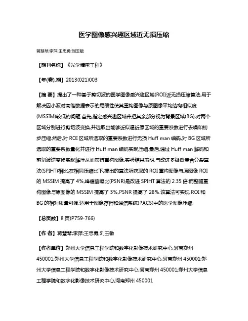
医学图像感兴趣区域近无损压缩蒋慧琴;李萍;王忠勇;刘玉敏【期刊名称】《光学精密工程》【年(卷),期】2013(021)003【摘要】提出了一种基于剪切波的医学图像感兴趣区域(ROI)近无损压缩算法,用于解决因小波对高维数据表示的局限性使其重构图像与原图像平均结构相似度(MSSIM)较低的问题.首先,指定感兴趣区域并把其余部分视为背景区域(BG);对两个区域分别进行剪切波变换,并选取出能够近似逼近原区域的重要系数进行去噪和初步压缩.然后,对ROI区域所选取的重要系数进行无损Huff man编码,对BG区域所选取的重要系数量化并进行Huff man编码实现压缩.最后,通过Huff man解码和剪切波逆变换实现解压从而获得重构图像.实验结果表明,与改进多级树集合分裂算法(SPIHT)相比,在相同压缩比下,提出的算法所获取的ROI重构图像与原图像ROI 的MSSIM提高了4%,峰值信噪比(PSNR)是改进SPIHT算法的2.35倍;而整幅重构图像与原图像的MSSIM提高了3%,PSNR提高了28%.该算法可实现ROI和BG的相对质量可调,适用于图像存档和通信系统(PACS)中的医学图像压缩.【总页数】8页(P759-766)【作者】蒋慧琴;李萍;王忠勇;刘玉敏【作者单位】郑州大学信息工程学院和数字化影像技术研究中心,河南郑州450001;郑州大学信息工程学院和数字化影像技术研究中心,河南郑州450001;郑州大学信息工程学院和数字化影像技术研究中心,河南郑州450001;郑州大学信息工程学院和数字化影像技术研究中心,河南郑州450001【正文语种】中文【中图分类】TP391.4;Q-334【相关文献】1.临床诊断学:形状自适应感兴趣区域医学图像无损压缩方法的研究 [J], 史贵连;叶福丽2.形状自适应感兴趣区域医学图像无损压缩方法的研究 [J], 史贵连;叶福丽3.基于感兴趣区域的医学图像近无损压缩 [J], 高尚兵;严云洋;梁燕;王晓燕;马岱4.基于感兴趣区域的医学图像近无损压缩 [J], 高尚兵;严云洋;梁燕;王晓燕;马岱5.基于感兴趣区域的医学图像近无损压缩 [J], 高尚兵;严云洋;梁燕;王晓燕;马岱因版权原因,仅展示原文概要,查看原文内容请购买。

保边滤波器:双边滤波与引导滤波保边滤波器(Edge Preserving Filter)是指在滤波过程中能够有效的保留图像中的边缘信息的⼀类特殊滤波器。
其中双边滤波器(Bilateral filter)、引导滤波器(Guided image filter)、加权最⼩⼆乘法滤波器(Weighted least square filter)为⼏种⽐较⼴为⼈知的保边滤波器。
双边滤波双边滤波很有名,使⽤⼴泛,简单的说就是⼀种同时考虑了像素空间差异与强度差异的滤波器,因此具有保持图像边缘的特性。
先看看我们熟悉的⾼斯滤波器其中W是权重,i和j是像素索引,K是归⼀化常量。
公式中可以看出,权重只和像素之间的空间距离有关系,⽆论图像的内容是什么,都有相同的滤波效果。
再来看看双边滤波器,它只是在原有⾼斯函数的基础上加了⼀项,如下其中 I 是像素的强度值,所以在强度差距⼤的地⽅(边缘),权重会减⼩,滤波效应也就变⼩。
总体⽽⾔,在像素强度变换不⼤的区域,双边滤波有类似于⾼斯滤波的效果,⽽在图像边缘等强度梯度较⼤的地⽅,可以保持梯度。
(1)中值滤波Fast Median and Bilateral FilteringWhat is GIMP’s equivalent of Photoshop’s Median filter?(2)双边滤波Bilateral Filtering for Gray and Color Images(3)导向滤波Guided Image Filtering(4)Bi-Exponential Edge-Preserving Smoother(5)选择性模糊(6)reference:。
![用于减少成像设备中极化作用的方法和装置[发明专利]](https://uimg.taocdn.com/53ac4a61680203d8cf2f2436.webp)
专利名称:用于减少成像设备中极化作用的方法和装置专利类型:发明专利
发明人:J·-P·布尼克,A·G·费什勒,H·阿尔特曼,U·德罗尔,I·布列维斯
申请号:CN200710149416.X
申请日:20070803
公开号:CN101116620A
公开日:
20080206
专利内容由知识产权出版社提供
摘要:提供了一种用于减少成像设备中极化作用的方法(250)和设备,并包括控制图像探测设备(100)的方法。
该方法包括施加热(252)到具有至少一个欧姆接触(200)的图像探测设备上并控制所施加的热以调整图像探测设备的温度水平。
申请人:GE医疗系统以色列有限公司
地址:以色列提拉特哈卡尔迈勒
国籍:IL
代理机构:中国专利代理(香港)有限公司
更多信息请下载全文后查看。
生物医学图像处理中常见滤波器的使用技巧生物医学图像处理是一个十分重要且广泛应用的领域,它在医疗诊断、研究分析等方面都发挥着重要作用。
而滤波器作为图像处理过程中不可或缺的一部分,也扮演着重要的角色。
在生物医学图像处理中,有一些常见的滤波器用于去除噪声、增强图像等。
接下来,我将介绍几种常见的滤波器以及它们的使用技巧。
1. 均值滤波器(Mean Filter)均值滤波器是一种常用的线性滤波器,它通过计算像素周围邻域的平均值来去除图像中的噪声。
在生物医学图像处理中,噪声可能来自于图像采集设备、传输过程或其他因素。
使用均值滤波器时,需要选择适当的滤波器尺寸,通常取3x3或5x5的大小。
较大的滤波器尺寸可以更好地平滑图像,但也会导致图像细节的丢失。
2. 中值滤波器(Median Filter)中值滤波器是一种非线性滤波器,它通过将像素周围邻域的像素值排序,然后取中间值作为滤波结果。
中值滤波器在去除图像中的椒盐噪声和斑点噪声时表现出色。
相比于均值滤波器,中值滤波器能够保留图像的细节信息,但也会导致一定程度的模糊。
3. 高斯滤波器(Gaussian Filter)高斯滤波器是一种在空域中进行滤波的线性平滑滤波器。
它通过计算像素周围邻域的加权平均值来降低图像中高频部分的强度,从而达到模糊图像的效果。
高斯滤波器通常用于平滑图像、去除高频噪声。
需要注意的是,滤波器尺寸和标准差的选择会对滤波结果产生影响。
较大的滤波器和较小的标准差将产生更强的平滑效果,但也会损失一些细节。
4. 锐化滤波器(Sharpening Filter)锐化滤波器用于增强图像的边缘和细节,使图像更加清晰。
常见的锐化滤波器包括拉普拉斯滤波器和增强锐化滤波器。
拉普拉斯滤波器对图像进行二阶微分,可以检测图像中的边缘。
增强锐化滤波器则通过将原始图像与锐化图像的加权和来增强边缘和细节。
在使用锐化滤波器时,需要注意控制增强的程度,避免过度增强导致图像噪声的增加。
专利名称:促进修正图像重建中的增益波动的方法和系统专利类型:发明专利
发明人:J·赫斯埃,C·A·博曼,J-B·蒂博,K·D·索尔
申请号:CN200780053171.9
申请日:20070531
公开号:CN101690418A
公开日:
20100331
专利内容由知识产权出版社提供
摘要:提供了用于重建图像的方法和系统。
该方法包括使用增益参数和偏移参数中的至少一个的联合估计以及重建图像的估计来执行断层摄影图像重建。
申请人:通用电气公司,普渡研究基金会,圣母大学
地址:美国纽约州
国籍:US
代理机构:中国国际贸易促进委员会专利商标事务所
代理人:张阳
更多信息请下载全文后查看。
2020年11月计算机工程与设计Nov. 2020第 41 卷 第 11 期 COMPUTER ENGINEERING AND DESIGNVol. 41 No. 11基于导向滤波的鬼影消除多曝光图像融合安世全,张莉+,瞿中(重庆邮电大学计算机科学与技术学院,重庆400065)摘 要:为解决传统多曝光融合算法存在光晕、细节丢失和鬼影消除不充分的问题,提出一种优化导向滤波的鬼影消除多 曝光融合算法。
为确保相似结构的像素存在相似的融合贡献,利用差分法和最大类间方差检测运动像素点;结合局部对比度、适当曝光度和色彩饱和度构建权重图;设计改进的导向滤波自适应地强化边缘区域,减少光晕,细化权重。
实验结果表明,该算法在边缘相似性和图像清晰度评价中平均提升31%和17%,运行效率至少提高23%,有效去除了鬼影和光晕, 呈现丰富的细节信4%关键词:图像融合;多曝光图像;鬼影消除;导向滤波;高动态范围中图法分类号:TP391. 41文献标识号:A 文章编号:1000-7024 (2020) 11315407doi : 10. 16208/j. issnl 000-7024. 2020. 11. 025Mult-exposure image fusion based on guided filtering andghostingremovelAN Sh-quan , ZHANG Li + , QU Zhong(College of Computer Science and Technology & Chongqing University of Posts and Telecommunications,Chongqing 400065 & China)Abstract : To address the phenomenon of halation, detail distortion and ghosting of moving objects in traditional mult-exposureimage fusion, a ghost-removal multi-exposure fusion algorithm based on improved guided filtering was proposed. The difference method and the maximum inter-class variance method wereusedtodetectmovingobjects , toensurethatpixelswithsimilar intensities and structures shared similar fusion weights. The initial exposure map was constructed with the local contrast, theappropriate exposure of the image and the color saturation. The improved guided filtering was used to adaptively enhance theedge regions & reduce halation and refine the weight map. The algorithm has the average increase of 31 % and 17% in edge simi larity and image clarity evaluation respectively, and the operating efficiency is increased by 23%. The proposed algorithm caneffectively remove ghost images and eliminate halation & and present rich details.Key words : image fusion ; multi-exposure image ; ghost elimination # guided filter ; high dynamic range0引言普通数码相机所捕获图像的动态范围远远低于现实场 景。
专利名称:基于梯度提取的单帧多光谱影像超分辨率重建方法及系统
专利类型:发明专利
发明人:王密,何鲁晓
申请号:CN201711367295.6
申请日:20171218
公开号:CN108090872A
公开日:
20180529
专利内容由知识产权出版社提供
摘要:本发明提供一种基于梯度提取的单帧多光谱影像超分辨率重建方法及系统,包括利用低通滤波将原始的单帧多光谱影像各波段从灰度图像转换为梯度图像,分离光谱信息与空间几何信息,选择一帧进行上采样作为参考梯度图;基于POCS算法框架,将其余梯度图像的信息投影到参考梯度图上,获得超分辨率梯度图;基于SFIM模型,根据超分辨率梯度图与原始的单帧多光谱影像实现信息融合,获得最终的超分辨率多光谱影像。
本发明可以有效克服数据量不足对超分辨率重建的影响,提高数据利用水平。
申请人:武汉大学
地址:430072 湖北省武汉市武昌区珞珈山武汉大学
国籍:CN
代理机构:武汉科皓知识产权代理事务所(特殊普通合伙)
代理人:严彦
更多信息请下载全文后查看。
专利名称:一种多光源快照的压缩X射线断层合成方法专利类型:发明专利
发明人:马旭,赵琦乐
申请号:CN202010303446.7
申请日:20200417
公开号:CN111652950A
公开日:
20200911
专利内容由知识产权出版社提供
摘要:一种多光源快照的压缩X射线断层合成方法,基于PRISM模型建立非线性CXT重构框架,然后提出一种改进的分裂布莱格曼算法求解非线性的逆向重构问题,从而获得被检测的三维物体图像;由于本发明允许多个光源同时照射物体,因此相比于传统的顺序照射方式,可以有效地缩短扫描时间,克服由于物体形变导致的图像失真问题,极大提高了重构算法对于物体运动或扰动的鲁棒性。
申请人:北京理工大学
地址:100081 北京市海淀区中关村南大街5号
国籍:CN
代理机构:北京理工大学专利中心
更多信息请下载全文后查看。
a rXiv:as tr o-ph/1673v15J un21Optimal multihump filter for photometric redshifts Tam´a s Budav´a ri 1,Alexander S.Szalay Department of Physics and Astronomy,The Johns Hopkins University,Baltimore,MD 21218budavari@ Istv´a n Csabai 2Department of Physics,E¨o tv¨o s University,Budapest,Pf.32,Hungary,H-1518Andrew J.Connolly Department of Physics and Astronomy,University of Pittsburgh,Pittsburgh,PA 15260and Zlatan Tsvetanov Department of Physics and Astronomy,The Johns Hopkins University,Baltimore,MD 21218ABSTRACT We propose a novel type filter for multicolor imaging to improve on the photomet-ric redshift estimation of galaxies.An extra filter—specific to a certain photometric system—may be utilized with high efficiency.We present a case study of the Hub-ble Space Telescope ’s Advanced Camera for Surveys and show that one extra exposure could cut down the mean square error on photometric redshifts by 34%over the z <1.3redshift range.Subject headings:galaxies:distances and redshifts —galaxies:photometry —instru-mentation:miscellaneous1.IntroductionThe prediction of photometric redshifts (Koo 1985;Connolly et al.1995a;Gwyn &Hartwick 1996;Sawicki,Lin &Yee 1997;Hogg et al.1998;Wang,Bahcall &Turner 1998;Yee 1998;Fern´a ndez-Soto,Lanzetta,&Yahil 1999;Weymann et al.1999;Ben´ıtez 2000;Csabai et al.2000;Budav´a riet al.2000)is built upon global continuum features of the underlying galaxy spectrum such as the Balmer break at4000˚A.The more precisely one can localize these features,the more accurate the redshift estimates become.However,traditional broadbandfilters were not designed to provide the best possible photometric redshifts,for several reasons.In theory,a set offilters optimal for photometric redshift estimation might be designed,but this would probably be substantially different from any current standard set.Here we do not intend to solve the generic problem of finding an optimalfilter set for photometric redshift estimation;this study shows how conventional filter sets can be extended to yield better photometric redshifts.In Section1.1,we present the idea of an additionalfilter and look into why and how an extra measurement—sampling the same wavelengths—can improve significantly on photometric redshifts.In Section2,the algorithm is developed and we make a case study of the Advanced Camera for Surveys of the Hubble Space Telescope.Based on our analysis,we propose a novel type of“broad-band”filter that can be effectively used for photometric redshifts.1.1.The ideaThe more general inversion problem of photometry in terms of redshift,type,and intrinsic luminosity(Koo1985;Connolly et al.1995a,b,1999;Budav´a ri et al.1999,2000;Csabai et al. 2000)involves the study of the Jacobian matrix offluxes as a function of the physical parameters of galaxies.Our numerical simulations show thatfilter sets yield more precise estimates when continuum spectral features are located around the overlap of two bands—bothfluxes change rapidly with redshift.One way to improve the redshift estimates is to increase the number of filters and use narrower bands.This would require too many exposures and yield a non-standard photometric system(Hickson et al.1998).The other possibility is to put an intermediate width (IM)filter in a broad band,which would help the redshift estimation by improving the resolution.A single IM band can only help in a narrow redshift range,so additional,narrowerfilters are needed for each broad band.This approach could triple the resolution but will heavily increase the total exposure time at the same signal-to-noise ratio.We propose combining multiple IMfilters located in standard photometric bands into one “broadband”filter.We call this a multihumpfilter.The resulting newfilter will be able to improve the redshift prediction(wavelength resolution)over a much wider redshift range and will only require a single additional exposure of comparable length.How does this really work?Our approach makes a large difference for blue galaxies.The4000˚A break in their spectra shows up only as a small“bump”which makes the redshift estimation difficult. Let us consider the worst-case scenario,a toy model spectrum of a late-type galaxy that declines with wavelength as a power law and has as its only spectral feature the approximately500˚A wide bump.Without this feature,the colors would be the same at any redshift.Theflux changes with redshift within a band depending on the shape of thefilter.If its gradient is too small(e.g.flatas a top-hat),tiny photometric errors can yield large errors in the redshift prediction.In other words,while the bump is in a broad band,it is hard to tell precisely where it is.The measured flux in our newfilter will change in redshift regions where the spectral feature is passing through one of the IM humps.These are the regions where the proposedfilter contributes the most to the redshift estimation and where the originalfilter set has poor performance(small gradient).Red elliptical(E/S0)galaxies do not present a significant problem,because the strong discontinuity at 4000˚A changes noticeably thefluxes as it passes through the bands with redshift.In this case the additionalfilter plays a subsidiary role,and the improvement of the accuracy is incremental.2.Filter designThe actual throughput of a photometric system strongly depends on the instrument,different projects use different CCDs to gain more sensitivity in the desired wavelength range.The quantum efficiency of these devices set strict constraints on the observable wavelength regime.Thefilter set is selected to cover the available spectral interval according to science goals.The multihumpfilter is specific to afilter set,and its transmissivity is affected by the CCD’s quantum efficiency(QE).We have analyzed the photometric system of the Hubble Space Telescope’s Advanced Camera for Surveys(ACS Ford et al.1996)3.The two back-illuminated CCDs of the widefield channel are VIS-AR coated in order to optimize the response in the I band,and thus the U-band sensitivity has been sacrificed.Mission specifications dictate the constraints on the multihumpfilter that is to extend the original set of the g’,r’,i’and z’bands,which span the entire observable wavelength range.No bluer or redderfilter can be used,because the detector is not sensitive at shorter or longer wavelengths.The framework of the algorithm is simple.We parameterize afictitiousfilter curve and convolve it with the CCD’s actual QE to obtain a realistic response function.Simulated photometric catalogs offluxes and errors are generated using the extendedfilter set.The goodness of a particularfilter set is assessed by computing the errors on the redshift estimates.In the context of currentfilter manufacturing techniques(Offer&Bland-Hawthorn1998),a feasible parameterization of the additionalfilter’s response function(R(λ),see Figure1)consists of at most two notchfilters,plus a low and a high cutoff,as described byR(λ)=1πarctan ǫ·(λ−λend)−exp − λ−λ1∆λ2 p .(1)Parametersλstart andλend are the limits of thefilter,andǫdetermines the gradients,the rise of the edges.The values ofλ1andλ2correspond to the locations of the notches and p(an even number)changes their shape.The mock catalogs were generated based on spectral energy distributions(SEDs)derived from a physical interpolation scheme applied to the spectra of Coleman,Wu&Weedman(1980),as described in Connolly et al.(1999)and Budav´a ri et al.(2000).On a high resolution redshift grid (δz=5×10⁻³),a hundred objects were generated at each grid point with random SEDs.The continuous type parameter was scaled to yield a population of galaxies in which the probability of having a spectral type between Ell and Sbc was10%,Sbc–Scd35%,Scd–Irr35%,and bluer 20%.Thefluxes were modulated with3%photometric errors taken from a Gaussian distribution. The quality of the photometric redshifts is determined by computing the rms of the estimates. The error is calculated for the desired redshift interval(or regions)meeting the actual project requirements—in this study,redshifts between z=0.2and z=1.2.The actual optimization problem has quite a few parameters(see Equation1)to solve for, which makes it hard to numericallyfind the global minimum.It is also quite time-consuming to evaluate the underlying function;a new loop of the simulation has to be completed each time.Also extra constraints were added to the problem.To be able to use the very samefilter from the ground for testing purposes or in follow-up observations,a design compromise due to the atmosphere has been made.In the actual optimization algorithm,one of the notches was always forced to include the5577˚A sky line.To map the entire parameter space,a linear search on a coarse grid was used tofind the best possiblefilter candidates,and then from the those minima,a gradient method was utilized with discrete,higher resolution step-sizes.3.DiscussionThe resulting shape of the multihump is shown in Figure2.This best configuration has two humps and its transmissivity peaks at the shortest possible wavelengths in the g’band and,at longer wavelength,in the i’band.Since the ACSfilters look almost like triangles(as a result of the strong wavelength dependency in the CCD’s QE),our additionalfilter tries to intensify the changes in colors,at the lowest,z∼0.2,and highest,z∼1.2,redshifts.On one side,the optimal multihumpfilter is essentially trying to compensate the lack of a ultravioletfilter by boosting the contrast at the edge of the g’band.In fact,the algorithm alsofinds an optimal solution of having a U band,which is not a real option because of the CCD’s QE(see Section2).The location of the hump in the i’is clearly set by the upper redshift limit z 1.2,when the Balmer break is at 8800˚A.Figure3compares the performance of the original and extendedfilter sets by plotting the rms error as a function of redshift.The accuracy of photometric redshifts for the entire catalog is shown first.The prediction improves at all redshifts;the overall improvement isσ2orig−σ2extQ=Early-and late-type subsamples are shown in the middle and right panels of Figure3,respectively. The E/S0estimates clearly get better at the smallest redshifts,z 0,and at around z 1.2,when the4000˚A break is in one of the humps.However,the redshift prediction also improves in another redshift region,around z∼0.55,as a result of the Hβand Mg i absorption as it passes through the second hump.In according with our expectations,redshift estimates of the late-type galaxies change much more drastically then those estimated for early types.The large number of parameters makes it difficult to estimate the errors or covariances.In Table1,the rms errors computed for different set offilters are shown.The original ACSfilter set givesσz=0.075.If we try additional multihumpfilters with humps centered on the g’r’i’and g’r’z’bands,the performance just slightly improves;σz=0.072and0.073,respectively.Centering humps on the gaps between the original bands(off-band multihumpfilter)does not improve on the accuracy of the estimates either;σz=0.073.The optimizedfilter yields much better redshifts,σz=0.058.The gain in the entire catalog is comparable to what would be achievable by using separate IMfilters.The redshift accuracy can be marginally increased by splitting the optimal multihump into two separatefilters(σz=0.055),but the additional exposure time would be more than twice as long as in our approach.4.ConclusionWe propose the use of multihumpfilters extending standard photometric systems to make photometric redshift estimation much more efficient.Our simulations have shown that an optimized extrafilter could improve the redshift prediction by34%for the Advanced Camera for Surveys. The improvement takes place over the z<1.3redshift range.Thefilter’s effective width is about 1500˚A,comparable to the existing photometric bands,so the measurement would require only about25%more exposure time.Such afilter can be built with today’s technology;in fact,similar filters have been utilized to suppres atmospheric features at near-infrared wavelengths(Offer& Bland-Hawthorn1998).The shape of the extrafilter can be tuned to different goals and missions. It can be optimized for differentfilter sets and adjusted to desired redshift ranges.I.C.and T.B.acknowledge partial support from the Hungarian Academy of Sciences–NSF grant124and the Hungarian National Scientific Research Foundation grant T030836,A.J.C.ac-knowledges support from NASA through a Long Term Space Astrophysics grant(NAG5-7934)and through grant GO-07817.06-96A from the Space Telescope Science Institute. A.S.acknowledges support from the NSF(AST98-02980)and the NASA Long Term Space Astrophysics program (NAG5-3503).REFERENCESBen´ıtez,N.,2000,ApJ,536,571Budav´a ri,T.,Szalay,A.S.,Connolly,A.J.,Csabai,I.&Dickinson,M.E.,1999,in Photometric Red-shifts and High Redshift Galaxies,eds.R.J.Weymann,L.J.Storrie–Lombardi,M.Sawicki, &R.Brunner,(San Francisco:ASP),19Budav´a ri,T.,Szalay,A.S.,Connolly,A.J.,Csabai,I.&Dickinson,M.E.,2000,AJ,120,1588Coleman,G.D.,Wu.,C.-C.,&Weedman,D.W.,1980,ApJS,43,393Connolly,A.J.,Csabai,I.,Szalay,A.S.,Koo,D.C.,Kron,R.G.,&Munn,J.A.,1995a,AJ,110, 2655Connolly,A.J.,Szalay,A.S.,Bershady,M.A.,Kinney,A.L.,&Calzetti,D.,1995b,AJ,110,1071Connolly,A.J.,Budav´a ri,T.,Szalay,A.S.,Csabai,I.,&Brunner,R.J.,1999,in Photometric Red-shifts and High Redshift Galaxies,eds.R.J.Weymann,L.J.Storrie–Lombardi,M.Sawicki, &R.Brunner,(San Francisco:ASP),13Csabai,I.,Connolly,A.J.,Szalay,A.S.,&Budav´a ri,T.,2000,AJ,119,69Fern´a ndez-Soto,A.,Lanzetta,K.M.,&Yahil,A.,1999,ApJ,513,34Ford,H.C.,et al.,1996,SPIE,2807,184Gwyn,S.D.J.,&Hartwick,F.D.A.,1996,ApJ,468,L77Hickson,P.,et al.,1998,SPIE,3352,226Hogg,D.W,et al.,1998,AJ,115,1418Koo,D.C.,1985,AJ,90,148Offer,A.R.,&Bland-Hawthorn,J.,1998,MNRAS,229,176Sawicki,M.J.,Lin,H.,&Yee,H.K.C,1997,AJ,113,1Wang,Y.,Bahcall,N.,&Turner,E.L.,1998,AJ,116,2081Weymann,R.J.,Storrie–Lombardi,L.J.,Sawicki,M.,&Brunner,R.,(editors),1999,Photometric Redshifts and High–Redshift Galaxies(San Francisco:ASP)Yee,H.K.C.,1998,in Proc.10th Recontres de Blois,in press(astro-ph/9809347)Table1.Errors on Photometric RedshiftsFilter Set∆z rmsλstartλendλ1∆λ1λ2∆λ2pǫFig.1.—Illustration of thefilter’s response curve,as defined by Equation1.Fig.2.—The throughput of thefilters as used in convolutions.The original g’,r’,i’,and z’bands are represented by solid lines(left to right).The add-on multihumpfilter(dotted line)is scaleddown by30%for illustration.Fig. 3.—The rms error on photometric redshifts using the originalfilter set(solid line)and the extended set(dotted line).Left to right:The improvement for the entire population in the simulation and for the red(E/S0)and blue subsamples,respectively.The large errors at lowredshifts are due to the lack of the U band;at redshift z>1,one would need a J band or higher.。