Analysis of RNA-Seq Data Using TopHat and Cufflinks
- 格式:pdf
- 大小:690.84 KB
- 文档页数:23
⼀步⼀步教你做转录组分析(HISAT,StringTieandBallgown)该分析流程主要根据2016年发表在Nature Protocols上的⼀篇名为Transcript-level expressionanalysis of RNA-seq experiments with HISAT, StringTie and Ballgown的⽂章撰写的,主要⽤到以下三个软件:HISAT (/software/hisat/index.shtml)利⽤⼤量FM索引,以覆盖整个基因组,能够将RNA-Seq的读取与基因组进⾏快速⽐对,相较于STAR、Tophat,该软件⽐对速度快,占⽤内存少。
StringTie(/software/stringtie/)能够应⽤流神经⽹络算法和可选的de novo组装进⾏转录本组装并预计表达⽔平。
与Cufflinks等程序相⽐,StringTie实现了更完整、更准确的基因重建,并更好地预测了表达⽔平。
Ballgown (https:///alyssafrazee/ballgown)是R语⾔中基因差异表达分析的⼯具,能利⽤RNA-Seq实验的数据(StringTie, RSEM, Cufflinks)的结果预测基因、转录本的差异表达。
然⽽Ballgown并没有不能很好地检测差异外显⼦,⽽ DEXseq、rMATS和MISO可以很好解决该问题。
⼀、数据下载Linux系统下常⽤的下载⼯具是wget,但该⼯具是单线程下载,当使⽤它下载较⼤数据时⽐较慢,所以选择axel,终端中输⼊安装命令:$sudo yum install axel然后提⽰输⼊密码获得root权限后即可⾃动安装,安装完成后,输⼊命令axel,终端会显⽰如下内容,表⽰安装成功。
Axel⼯具常⽤参数有:axel [选项][下载⽬录][下载地址]-s :指定每秒下载最⼤⽐特数-n:指定同时打开的线程数-o:指定本地输出⽂件-S:搜索镜像并从X servers服务器下载-N:不使⽤代理服务器-v:打印更多状态信息-a:打印进度信息-h:该版本命令帮助-V:查看版本信息号#Axel安装成功后在终端中输⼊命令:$axel ftp:///pub/RNAseq_protocol/chrX_data.tar.gz此时在终端中会显⽰如下图信息,如果不想该信息刷屏,添加参数q,采⽤静默模式即可。
作物学报 ACTA AGRONOMICA SINICA 2020, 46(7): 1016 1024 / ISSN 0496-3490; CN 11-1809/S; CODEN TSHPA9 E-mail: zwxb301@本研究由国家重点研发计划项目(2016YFD0101002)和中国农业科学院创新工程专项经费资助。
This work was supported by the National Key Research and Development Program of China (2016YFD0101002) and the Agricultural Science and Technology Innovation Program of Chinese Academy of Agricultural Sciences.*通信作者(Corresponding author): 郑军, E-mail: zhengjun02@ **同等贡献(Contributed equally to this work)第一作者联系方式: 任蒙蒙, E-mail: ren_mm1991@; 张红伟, E-mail: zhanghongwei@Received (收稿日期): 2019-10-12; Accepted (接受日期): 2020-04-15; Published online (网络出版日期): 2020-04-26. URL: /kcms/detail/11.1809.S.20200426.1458.016.htmlDOI: 10.3724/SP.J.1006.2020.93054玉米耐深播主效QTL qMES20-10的精细定位及差异表达基因分析任蒙蒙1,** 张红伟1,** 王建华2 王国英1 郑 军1,*1中国农业科学院作物科学研究所, 北京100081; 2 中国农业大学农学院, 北京100193摘 要: 干旱是影响玉米(Zea mays L.)产量最主要的环境因素之一, 具有耐深播特性的玉米种质材料能够吸收土壤深层水分, 具有较强的耐旱性, 因此研究玉米耐深播性状的遗传机制具有重要的理论和应用价值。
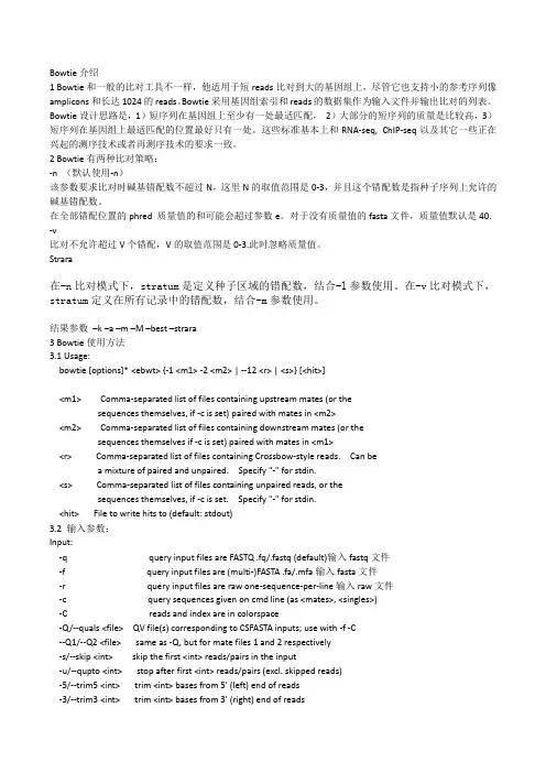
Bowtie介绍1 Bowtie和一般的比对工具不一样,他适用于短reads比对到大的基因组上,尽管它也支持小的参考序列像amplicons和长达1024的reads。
Bowtie采用基因组索引和reads的数据集作为输入文件并输出比对的列表。
Bowtie设计思路是,1)短序列在基因组上至少有一处最适匹配,2)大部分的短序列的质量是比较高,3)短序列在基因组上最适匹配的位置最好只有一处。
这些标准基本上和RNA-seq, ChIP-seq以及其它一些正在兴起的测序技术或者再测序技术的要求一致。
2 Bowtie有两种比对策略:-n (默认使用-n)该参数要求比对时碱基错配数不超过N,这里N的取值范围是0-3,并且这个错配数是指种子序列上允许的碱基错配数。
在全部错配位置的phred 质量值的和可能会超过参数e。
对于没有质量值的fasta文件,质量值默认是40. -v比对不允许超过V个错配,V的取值范围是0-3.此时忽略质量值。
Strara在-n比对模式下,stratum是定义种子区域的错配数,结合-l参数使用。
在-v比对模式下,stratum定义在所有记录中的错配数,结合-m参数使用。
结果参数–k –a –m –M –best –strara3 Bowtie使用方法3.1 Usage:bowtie [options]* <ebwt> {-1 <m1> -2 <m2> | --12 <r> | <s>} [<hit>]<m1> Comma-separated list of files containing upstream mates (or thesequences themselves, if -c is set) paired with mates in <m2><m2> Comma-separated list of files containing downstream mates (or thesequences themselves if -c is set) paired with mates in <m1><r> Comma-separated list of files containing Crossbow-style reads. Can bea mixture of paired and unpaired. Specify "-" for stdin.<s> Comma-separated list of files containing unpaired reads, or thesequences themselves, if -c is set. Specify "-" for stdin.<hit> File to write hits to (default: stdout)3.2 输入参数:Input:-q query input files are FASTQ .fq/.fastq (default)输入fastq文件-f query input files are (multi-)FASTA .fa/.mfa输入fasta文件-r query input files are raw one-sequence-per-line输入raw文件-c query sequences given on cmd line (as <mates>, <singles>)-C reads and index are in colorspace-Q/--quals <file> QV file(s) corresponding to CSFASTA inputs; use with -f -C--Q1/--Q2 <file> same as -Q, but for mate files 1 and 2 respectively-s/--skip <int> skip the first <int> reads/pairs in the input-u/--qupto <int> stop after first <int> reads/pairs (excl. skipped reads)-5/--trim5 <int> trim <int> bases from 5' (left) end of reads-3/--trim3 <int> trim <int> bases from 3' (right) end of reads--phred33-quals input quals are Phred+33 (default)默认质量值--phred64-quals input quals are Phred+64 (same as --solexa1.3-quals)--solexa-quals input quals are from GA Pipeline ver. < 1.3--solexa1.3-quals input quals are from GA Pipeline ver. >= 1.3--integer-quals qualities are given as space-separated integers (not ASCII)Tophat调用bowtie使用的输入参数是-q 。

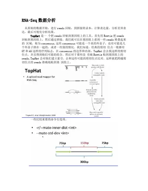
RNA-Seq数据分析从原始的数据开始,进行reads回帖,到拼接转录本,计算表达量,分析差异表达,最后可视化分析结果。
TopHat是一个把reads回帖到基因组上的工具。
首先用Bowtie把reads 回帖到基因组上,然后通过拼接,我们就可以在基因组上看到一些reads堆叠起来的区域,称为consensus,这些consensus可能是一个真的外显子,也有可能是几个外显子拼在一起的,或者一些别的情况。
我们知道,经典的剪切位点一般都有GT和AG这样的序列标志,在consensus的边界和内部,TopHat会去找这样的剪切位点,并且得到他们可能的组合。
然后对于那些没有被Bowtie贴到基因组上的reads,TopHat会对他们建立索引,去和这些可能的剪切位点比对,这样就把跨越剪切位点的reads准确地贴到基因组上。
一些比较重要的命令行选项。
关于插入片段长度的选项:在RNA-Seq中,会把mRNA打断成小的片段,然后对片段长度进行iding筛选后拿去测序,如果选择的片段长度是300bp,两端各测序75bp的reads,中间的插入片段长度就应该设为150bp.下面是设置插入片段长度的标准差,如果选择的片段长度比较集中,这个值可以设置的小一些,反之应该设置得大一些。
-G选项是提供哦呢一个已有的注释文件。
如果你分析的基因组被注释得比较好了,最好能够提供这个文件,这时TopHat就会先把reads往转录组上贴,没有贴到转录组上的再往基因组上贴,最后把结果合并起来。
我们知道大多数的转录组都是比基因组小得多的,而且junction reads可以直接贴到转录本上,所以这样回帖的效力和准确度都可以得到提高。
标准的Illumina平台是不分链的,我们无法知道配对的reads哪个方向和转录本一致,哪个和转录本反向互补。
对于分链的数据,也有两种情况,在firststrand这种分链方法中,第二个read和转录本方向一致,第一个read和转录本反向互补,在另一种fr- secondstrand分链方法中,就刚好反过来了。
TopHat2 是一个用于分析RNA-Seq 数据的常用软件工具。
它被用于检测基因表达水平、发现新的转录本和剪接变异等任务。
以下是TopHat2 的基本用法:1. 安装TopHat2:首先,你需要从TopHat2 的官方网站或适当的资源中下载和安装TopHat2 软件包。
按照官方提供的安装说明进行安装。
2. 准备参考基因组:在运行TopHat2 之前,你需要准备一个参考基因组序列和相应的注释文件。
参考基因组可以是已知的物种基因组序列,可以从公共数据库中下载或自行构建。
注释文件可以是GFF 格式或GTF 格式的文件,提供基因和转录本的注释信息。
3. 运行TopHat2:在命令行终端中输入以下命令来运行TopHat2:tophat2 [options] <index> <reads1.fastq> [reads2.fastq]其中,`<index>` 是指准备好的参考基因组索引文件的路径;`<reads1.fastq>` 和`[reads2.fastq]` 是输入的RNA-Seq 测序数据文件的路径,如果是单末端测序,只需提供`<reads1.fastq>`。
可选的参数可以用来设置比对的参数和其他选项,例如指定输出目录、选择比对器、指定线程数等。
你可以通过输入`tophat2 --help` 查看完整的参数列表和说明。
4. 解析结果:TopHat2 运行完成后,将生成BAM 格式的比对结果文件。
你可以使用其他工具(例如Samtools)来处理和解析BAM 文件,例如生成比对统计信息、计算基因表达水平或进行转录本分析等。
请注意,以上是TopHat2 的基本用法概述。
在实际使用中,你可能需要根据具体的研究目的和数据特点进行更详细的参数设置和分析流程。
建议参考TopHat2 的官方文档和相关资源以获取更多详细信息和使用示例。
基迪奥干货分享精选生物信息学实用工具与教pdf版生物信息学是一个富有挑战性和前景广阔的领域,它的迅速发展和进步使得生命科学研究水平得到了极大的提高。
作为生物信息学工作人员,我们需要不断地学习新的工具和技术,以提高我们的分析能力和研究效率。
以下是一些我个人整理的生物信息学实用工具与教程分享,希望能对大家的工作有所帮助。
一、生物信息学实用工具1. TopHatTopHat是一款常用的RNA-Seq分析软件,由Trapnell等人开发。
它可以在除去呈现类似重复子结构的转录本和基因组重复区域后将RNA-Seq数据比对到基因组上。
TopHat还可以考虑跨越内含子的原始测序数据,并生成新的转录本拼接图。
2. HISAT2HISAT2是一款专门用于RNA-Seq数据比对的工具,由Bowtie作者开发。
相较于其他工具,HISAT2具有更高的比对速度和更少的假阳性,可以提高RNA-Seq数据的精度和可靠性。
3. GATKGATK是一个广泛使用的基因组分析工具箱,它可以用于SNP和INDEL标记、组装、重排序、去重、宏观变异检测、联合分析等多个领域。
GATK针对人类基因组的分析更为精确和灵敏。
它通常在全基因组分析和重测序分析中使用。
4. FastQCFastQC是一款免费的软件工具,可以对Illumina测序数据质量进行快速检查,例如读数质量、测序深度、GC含量等。
FastQC可以在测序数据处理的各个阶段中使用,以保证数据的可靠性和准确性。
5. BWABWA是一款高效的基因组比对工具,从较长高质量的reads序列参考基因组序列。
它可以实现基因组比对的精确、高速计算,通常用于对祖先基因组测序和人类疾病相关的基因寻变分析等。
二、生物信息学实用教程1.生物信息学基础本课程介绍了常见的生物信息学数据库及其应用,包括NCBI、Ensembl、KEGG、GO等。
该教程重点讲述了如何储存和查询生物学信息,包括数据下载和基本的数据处理和排序方法。
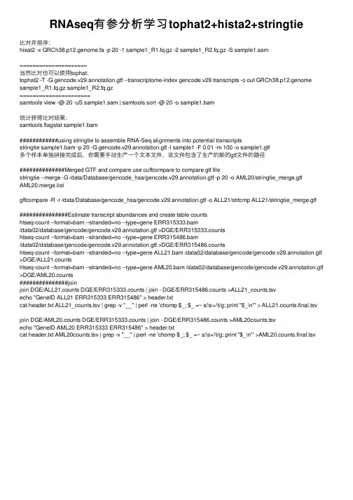
RNAseq有参分析学习tophat2+hista2+stringtie⽐对并排序:hisat2 -x GRCh38.p12.genome.fa -p 20 -1 sample1_R1.fq.gz -2 sample1_R2.fq.gz -S sample1.sam=====================当然⽐对也可以使⽤tophat:tophat2 -T -G gencode.v29.annotation.gtf --transcriptome-index gencode.v29.transcripts -o out GRCh38.p12.genome sample1_R1.fq.gz sample1_R2.fq.gz======================******************************|*****************************统计获得⽐对结果:samtools flagstat sample1.bam############using stringtie to assemble RNA-Seq alignments into potential transcriptsstringtie sample1.bam -p 20 -G gencode.v29.annotation.gtf -l sample1 -F 0.01 -m 100 -o sample1.gtf多个样本单独拼接完成后,你需要⼿动⽣产⼀个⽂本⽂件,该⽂件包含了⽣产的新的gtf⽂件的路径##############Merged GTF and compare use cuffcompare to compare gtf filestringtie --merge -G /data/Database/gencode_hsa/gencode.v29.annotation.gtf -p 20 -o AML20/stringtie_merge.gtfAML20.merge.listgffcompare -R -r /data/Database/gencode_hsa/gencode.v29.annotation.gtf -o ALL21/strtcmp ALL21/stringtie_merge.gtf ###############Estimate transcript abundances and create table countshtseq-count --format=bam --stranded=no --type=gene ERR315333.bam/data02/database/gencode/gencode.v29.annotation.gtf >DGE/ERR315333.countshtseq-count --format=bam --stranded=no --type=gene ERR315486.bam/data02/database/gencode/gencode.v29.annotation.gtf >DGE/ERR315486.countshtseq-count --format=bam --stranded=no --type=gene ALL21.bam /data02/database/gencode/gencode.v29.annotation.gtf >DGE/ALL21.countshtseq-count --format=bam --stranded=no --type=gene AML20.bam /data02/database/gencode/gencode.v29.annotation.gtf >DGE/AML20.counts###############joinjoin DGE/ALL21.counts DGE/ERR315333.counts | join - DGE/ERR315486.counts >ALL21_counts.tsvecho "GeneID ALL21 ERR315333 ERR315486" > header.txtcat header.txt ALL21_counts.tsv | grep -v "__" | perl -ne 'chomp $_; $_ =~ s/\s+/\t/g; print "$_\n"' > ALL21.counts.final.tsv join DGE/AML20.counts DGE/ERR315333.counts | join - DGE/ERR315486.counts >AML20counts.tsvecho "GeneID AML20 ERR315333 ERR315486" > header.txtcat header.txt AML20counts.tsv | grep -v "__" | perl -ne 'chomp $_; $_ =~ s/\s+/\t/g; print "$_\n"' >AML20.counts.final.tsv。
RNA序列分析和功能预测方法在生物学领域,RNA序列分析和功能预测是研究RNA分子的重要组成部分。
随着高通量测序技术的发展,越来越多的RNA序列数据被生成和积累,因此,开发高效准确的RNA序列分析和功能预测方法变得尤为重要。
本文将介绍RNA序列分析的基本步骤和一些常用的功能预测方法。
RNA序列分析的基本步骤通常包括数据质量控制、序列比对和注释。
数据质量控制是第一步,它用来筛选和排除低质量的测序数据。
在这个阶段,需要对数据进行质量评估、去除低质量的碱基以及去除可能的污染序列。
常用的软件工具如FastQC和Trimmomatic可用于数据质量控制的处理。
序列比对是RNA序列分析的关键步骤,它用来将目标序列与已知的参考序列进行比较,以确定相似性和差异性。
最常用的序列比对算法是Smith-Waterman和BLAST (Basic Local Alignment Search Tool)。
Smith-Waterman算法适合于短序列的比对,而BLAST算法适用于长序列的比对。
此外,还有一些软件工具如Bowtie、HISAT2和STAR等,它们对于高通量测序数据的比对速度更快且更准确。
注释是对比对后的序列进行进一步的功能分析,以确定序列中的基因或非编码RNA的功能。
注释步骤包括基因识别、转录组组装和功能注释。
基因识别是用来从比对序列中识别出编码蛋白质的基因。
转录组组装是将测序数据组装成转录本,即识别不同的转录变体。
功能注释是根据已知的功能和路径信息对转录本进行注释,以预测其在生物学过程中的作用。
常用的注释工具包括Cufflinks、StringTie和TopHat 等。
功能预测是根据RNA序列的特征和已知的功能信息来预测RNA分子的功能。
功能预测方法种类繁多,其中一些常用的方法包括同源性比较、表达式分析和RNA结构预测。
同源性比较是一种常用的功能预测方法,它通过比较目标序列与已知功能的序列之间的相似性来预测目标序列的功能。
rna速率计算公式理解RNA速率计算公式是用来计算RNA合成速率的公式。
在生物学研究中,RNA合成速率是指单位时间内RNA分子的合成数量。
RNA合成速率的计算涉及到不同的实验技术和方法,以下将从转录速率和测序数据分析两个方面简要介绍RNA速率计算公式的理解和相关参考内容。
1. 转录速率的计算公式:RNA转录速率的计算是通过实验测量转录程度以及mRNA的稳定性来确定的。
其中转录程度通常使用测量RNA的增长速率来表示,而mRNA稳定性可以通过添加转录抑制剂或抑制RNA降解途径来测量。
转录速率的计算公式如下:转录速率 = RNA增长速率 / mRNA稳定性其中,RNA增长速率可以通过实验测量RNA的合成速率得到,mRNA稳定性可以通过实验测量RNA的半衰期来得到。
具体测量技术包括核酸荧光标记、RT-qPCR、RNA测序等。
相关参考内容如下:- Nagalakshmi, U., Wang, Z., Worley, K. C., et al. (2008). The Transcriptional Landscape of the Yeast Genome Defined by RNA Sequencing. Science, 320(5881), 1344–1349.doi:10.1126/science.1158441- Garcia-Martinez, J., Aranda, A., & Perez-Ortin, J. E. (2004). Genomic run-on evalu- lates transcription rates for all yeast genes and identifies gene regulatory pro- gramming. Molecular Cell,15(2), 303–313. doi:10.1016/j.molcel.2004.06.004- Efroni, S., Duttagupta, R., Cheng, J., et al. (2008). Global Transcription in Plu- ripotent Embryonic Stem Cells. Cell Stem Cell, 2(5), 437–447. doi:10.1016/j. stem.2008.03.012以上参考内容提供了RNA转录速率的计算方法和实验技术的具体应用,可以帮助读者更好地理解RNA速率的计算公式。
RNA-seq中的基因表达量计算和表达差异分析RNA-seq中的基因表达量计算和表达差异分析差异分析的步骤:1)⽐对;2) read count计算;3) read count的归⼀化;4)差异表达分析;背景知识:1)⽐对:普通⽐对: BWA,SOAP开⼤GAP⽐对:Tophat(Bowtie2);2) Read count(多重⽐对的问题):丢弃平均分配利⽤Unique region估计并重新分配表达量计算的本质⽬标基因表达量相对参照系表达量的数值。
参照的本质:( 1)假设样本间参照的信号值应该是相同的;( 2)将样本间参照的观测值校正到同⼀⽔平;( 3)从参照的数值,校正并推算出其他观测量的值。
例如:Qpcr:⽬标基因表达量(循环数)相对看家基因表达量(循环数);RNA-seq:⽬标基因的表达量(测序reads数),相对样本RNA总表达量(总测序量的reads数),这是最常⽤的标准。
归⼀化的原因及处理原则:1)基因长度2)测序量3)样本特异性(例如,细胞mRNA总量,污染等)前两者使⽤普通的RPKM算法就可以良好解决,关键是第三个问题,涉及到不同的算法处理。
RNA-Seq归⼀化算法的意义:基因表达量归⼀化:在⾼通量测序过程中,样品间在数据总量、基因长度、基因数⽬、⾼表达基因分布甚⾄同⼀个基因的不同转录本分布上存在差别。
因此不能直接⽐较表达量,必须将数据进⾏归⼀化处理。
RNA-seq差异表达分析的⼀般原则1)不同样品的基因总表达量相似2)上调差异表达与下调差异表达整体数量相似(上下调差异平衡)3)在两组样品中不受处理效应影响的基因,表达量应该是相近的(差异不显著)。
4)看家基因可作为表达量评价依据(待定)不同的算法⽐较:以什么数值来衡量表达量:RPKM、FPKM、TPM以什么作为参照标准:TMM(edgeR软件)、De seq矫正RPKM:是Reads Per Kilobase per Million mapped reads的缩写,代表每百万reads中来⾃于某基因每千碱基长度的reads数。
RNAseq定量分析方案RNAseq定量分析方案 1一、实验目的: 2二、实验大致流程 2三、实验前的准备活动 23.1准备数据 23.2确定涉及软件是否安装完毕,及其输入输出文件。
3四、实验过程 44.1.利用bowtie2-bulid命令根据提供的参考基因组序列建立对应的索引文件。
54.2.利用tophat命令将分别将代比较的reads maping到参考基因组序列上 64.3利用cufflinks软件分别将待测样品的转录组reads拼接起来,并同时计算每个样品各个基因的rpkm值 74.4.利用coffmerge和cuffdiff软件计算每个样品各个基因的fpkm值。
8五.利用R软件查看结果文件。
10一、实验目的:利用已有的水稻基因组数据对来自两棵不同的水稻进行转录组水平差异的研究。
二、实验大致流程1. 利用bowtie2-bulid命令根据提供的参考基因组序列建立对应的索引文件2. 利用tophat命令将分别将代比较的reads maping到参考基因组序列上3. 利用cufflinks软件分别将待测样品的转录组reads拼接起来,计算每个样品各个基因的fpkm值4. 利用coffmerge和cuffdiff软件计算每个样品各个基因的fpkm值。
5. 利用R软件查看比较结果。
三、实验前的准备活动3.1准备数据像大多数生物实验一样,做生物信息学实验之前也是需要事先准备好“药品”和“仪器”,不然到了关键时刻也是一样会手忙脚乱的。
现在我们先来谈一谈生物信息实验需要准备的“药品”—数据。
对于RNAseq实验而言,这里至少需要准备一下几个文件:1.参考基因组序列文件如 refrence.fa参考基因组数据:2.参考基因组注释文件如 refrence.gtfa参考基因组序列设为refrence.fa b参考基因注释设为refrence.gtfF1_sample_R1.fastq待比较样品F1:(为RNA测序数据) F1_sample_R1.fastqP1_sample_R1.fastq待比较样品P2:(为RNA测序数据) P1_sample_L007_R2.fastq3.2确定涉及软件是否安装完毕,及其输入输出文件。
转录组分析学习笔记(持续补充)转录组分析流程(有参和⽆参de novo)1. 获得测序数据,Fastq格式,称之为Raw data。
2. 质量检测3. ⽐对Mapping4. Quantification|Quantitation5. 差异表达分析补充:开始项⽬之前,先确⽴合理的⽂件⽬录结构。
【1】Raw Data 处理理论知识⾼通量测序之所以能够能够达到如此⾼的通量的原因就是他把原来⼏⼗M,⼏百M,甚⾄⼏个G的基因组通过物理或化学的⽅式打算成⼏百bp的短序列,然后同时测序。
在测序过程中,机器会对每次读取的结果赋予⼀个值,⽤于表明它有多⼤把握结果是对的。
从理论上都是前⾯质量好,后⾯质量差。
并且在某些GC⽐例⾼的区域,测序质量会⼤幅度降低。
因此,我们在正式的数据分析之前需要对分析结果进⾏质控。
Fastq ⽂件测序给的“原始数据”,称之为Raw Data。
FASTQ是基于⽂本的,保存⽣物序列(通常是核酸序列)和其测序质量信息的标准格式。
其序列以及质量信息都是使⽤⼀个ASCII字符标⽰,最初由Sanger开发,⽬的是将FASTA序列与质量数据放到⼀起,⽬前已经成为⾼通量测序结果的事实标准。
FASTQ⽂件中以四⾏最为⼀个基本单元,并对应⼀条序列的测序信息,各⾏记录信息如下:第⼀⾏记录序列标识以及相关的描述信息,以‘@’开头,为了保证后续分析软件能够区分每条序列,单个序列的标识必须具有唯⼀性;第⼆⾏为碱基序列;第三⾏以‘+’开头,后⾯是序列标⽰符、描述信息,或者什么也不加;第四⾏,是质量信息,长度和第⼆⾏的序列相对应,每⼀个序列都有⼀个质量评分,根据评分体系的不同,每个字符的含义表⽰的数字也不相同。
碱基质量得分与错误率的换算关系: Q = -10log10p(p表⽰测序的错误率,Q表⽰碱基质量分数)ASCII值与碱基质量得分之间的关系:Phred64 Q=ASCII转换后的数值-64Phred33 Q=ASCII转换后的数值-33⽬前illumina使⽤的碱基质量格式为phred+33, 和Sanger的质量基本⼀致(⽼数据建议查看清楚再进⾏后续处理)。
C hapter 18A nalysis of RNA-Seq Data Using TopHat and Cuffl inksS reya G hosh and C hon-Kit K enneth C hanA bstractT he recent advances in high throughput RNA sequencing (RNA-Seq) have generated huge amounts of data in a very short span of time for a single sample. These data have required the parallel advancement of computing tools to organize and interpret them meaningfully in terms of biological implications, at the same time using minimum computing resources to reduce computation costs. Here we describe the method of analyzing RNA-seq data using the set of open source software programs of the Tuxedo suite: TopHat and Cuffl inks. TopHat is designed to align RNA-seq reads to a reference genome, while Cuffl inks assembles these mapped reads into possible transcripts and then generates a fi nal transcriptome assembly. Cuffl inks also includes Cuffdiff, which accepts the reads assembled from two or more biological conditions and analyzes their differential expression of genes and transcripts, thus aiding in the investigation of their transcriptional and post transcriptional regulation under different conditions. We also describe the use of an accessory tool called CummeRbund, which processes the output fi les of Cuffdiff and gives an output of publication quality plots and fi gures of the user’s choice. We demonstrate the effectiveness of the Tuxedo suite by analyzing RNA-Seq datasets of A rabidopsis thaliana root subjected to two different conditions.K ey words R NA-seq ,B owtie ,T opHat ,C uffl inks ,C uffmerge ,C uffcompare ,C uffdiff ,C ummeRbund ,D ifferential gene expression ,T ranscriptome assembly1I ntroductionI n the early years of transcriptome studies, microarray technologiesbased on nucleic acid hybridization were predominately used forgene expression analysis. However, these technologies posed a lim-itation in quantifying the various kinds of RNA molecules that areexpressed by the genome under myriad biological conditions atdifferent points of time. The limitation is mainly due to the reli-ance on extensive prior knowledge of the genome [ 1]. The recentadvances in Next Generation Sequencing (NGS) of DNA [ 2] haveled to a burst in RNA analysis through massively parallel cDNAsequencing that has accelerated our understanding of the dynamicsof genome expression and genome structural variation [ 1,3,4].Methods have also been devised to directly sequence RNA on amassively parallel scale without intermediate cDNA generation [ 5] David Edwards (ed.), Plant Bioinformatics: Methods and Protocols, Methods in Molecular Biology, vol. 1374,DOI 10.1007/978-1-4939-3167-5_18, © Springer Science+Business Media New York 2016339340in order to avoid some of the pitfalls or artifacts produced during cDNA synthesis from RNA strands [ 6 ], producing reads which are bias free and more comprehensive. High throughput R NA-seq produces large volumes of data in a single experiment, which need to be assembled correctly in order to interpret them meaningfully. A large number of computation methods and tools have been developed for effi cient assembly, quantifi cation, and differential analysis of such data [ 7 ]. Of these the “Tuxedo suite” of pro-grams— B owtie , T opHat , and C uffl inks —along with accessory tools and programs, like C ummeRbund , have gained a lot of popu-larity. The TopHat algorithm maps sequenced reads to a reference genome without relying on prior annotation of genes and accounts for alternative splicing of a primary transcript, while the Cuffl inks algorithm estimates transcript abundances and differential expres-sion. Analysis of large volumes of RNA-seq data with these algo-rithms has revealed novel isoforms and splice variants, as well as unannotated transcripts even in well studied biological models [ 8 ]. T he transcriptomic profi le of an organism at any given time orcondition gives the set of all its transcripts and their quantities pres-ent at the specifi c time point or condition. The transcriptome reveals a great deal about the functional aspects of the genome as well as the different kinds of biomolecules present within the cell or tissue. It is also very useful for studying the genetics behind growth, development and disease. Transcriptome studies aim at cataloging the different kinds of RNA in an organism, and quanti-fying the changes in expression levels of individual transcripts with time or under certain conditions [ 9 ]. Previously, there have been two approaches for sequencing RNA: (a) The hybridization based approach which involved the use of microarrays [ 10 , 11 ] and (b) The sequencing approach which directly determined the cDNA sequence using Sanger Sequencing approaches. The latter approach developed as an alternative to microarray technology, because hybridization heavily relied upon known sequenced genes and genomic regions. As sequencing the whole cDNA segment to pro-duce ESTs is expensive and has huge limitations when quantifying expressions, many tag based high throughput sequence approaches were developed for expression quantifi cation. These included CAGE (Cap Analysis of Gene Expression) [ 12 , 13 ], SAGE (Serial Analysis of Gene Expression) [ 14 ], and MPSS (Massively Parallel Signature Sequencing) [ 15 , 16 ]. The advancement of high throughput NGS technology makes the R NA-seq technology fea-sible and affordable for transcriptome profi ling. RNA-seq involves extracting the total RNA from a sample, then selecting an RNA population subset (such as poly A (+)), converting them to cDNA, and ligating the cDNA to specifi c adaptors at one or both ends of the fragment. These modifi ed fragments are then sequenced from one (single end sequencing) or both ends (paired end sequencing), with or without amplifi cation, in a high throughput NGS1.1R NA-seq Sreya Ghosh and Chon-Kit Kenneth Chan341sequencing machine. After sequencing, the RNA reads are mapped and quantifi ed based on a reference genome [ 17 ]. If a reference genome is not available, de novo transcriptome assembly can be carried out [ 18 ]. The RNA-seq analysis is also good for determin-ing spliced junctions with the resolution of a single base, determin-ing the structural variations in the genome, and locating transcript boundaries and novel genes and transcripts [ 9 ]. However, there are weaknesses in the RNA-seq technology. For example, DNA artifacts can be synthesized during cDNA cloning and that could cause misinterpretations later on. This weakness can be remediated by carrying out RNA-seq in replicates to even out the differences or account for sample variability during analysis [ 6 , 7 ]. For a com-prehensive review of RNA-seq, it is recommended to review the paper by Wang et al. [ 9 ]. R NA-seq data are usually very large and require effi cient algorithms which use minimum computing resources for their analysis.T here are three main steps in the reference-based R NA-seq analysis [ 7 ]:1. A ligning R NA-seq reads to a reference genome or transcriptome.2. A ssembling the aligned reads into transcription units, or recon-struction of a transcriptome.3. P erforming differential expression of transcripts across differ-ent conditions or time pointsE ach of the three steps possesses different computation chal-lenges [ 7 ]. Although there are several different algorithms and tools that address each of these challenges separately, in this chap-ter, we only illustrate the popular Tuxedo Suite which contains a comprehensive set of programs that perform reference-based R NA-seq analysis effi ciently. The core programs for RNA-seq anal-ysis in the Tuxedo suite are:1. B owtie [ 19 ], an ultrafast unspliced read aligner with high memory effi ciency. It uses the Burrows Wheeler Transform[ 20 ] and FM indexing [ 21 ] to compact a reference genome into a data structure that is effi cient for aligning short reads with perfect matches.2. T opHat [ 22 ] uses an “exon fi rst” approach to align reads. It uses B owtie to map the short contiguous unspliced reads to a reference genome. The unmapped reads are then split into shorter fragments and then are aligned independently to iden-tify splice junctions between exons.3. C uffl inks [ 23 ] uses the alignment fi le from T opHat , or other aligners which allow spliced alignments, to assemble and reconstruct the transcriptome. It assembles the overlapping “bundles” of aligned reads into transcripts using a probabilistic 1.2 T he Tuxedo Suiteof Computational Tools Analysis of RNA-Seq Data Using TopHat and Cuffl inks342approach, then merges multiple conditions and estimates the transcript abundances using C uffmerge and C uffcompare respectively ( s ee N ote 9 ). It can also useC uffdiff to calculate the differential gene expression.4. F inally, an accessory tool,C ummeRbund [ 24 , 23 ], renders the C uffdiff output into visual representations like bar, scatter and volcano plots.T he Tuxedo suite programs are all run in the command line. Alternatively, the web-based platform, Galaxy [25 ], provides a bet-ter user friendly interface to run the Tuxedo suite programs but the free public Galaxy server is limited to analysis of smaller datasets.T he Tuxedo suite provides a comprehensive workfl ow for R NA- seq analysis. There are a number of alternative packages and tools that can be used in conjunction with or as an alternative to any ofthe tools in the Tuxedo suite. For example there are many otherunspliced read aligners like SHRiMP [26 ] and Stampy [ 27 ] that follow the seed method and Smith–Waterman extension to align unspliced reads to the genome with high accuracy, and splicedaligners like MapSplice [28 ] and GSNAP [ 29 ]. There are also transcriptome assemblers like Scripture [30 ] (which is similar to C uffl inksbut uses a segmentation approach) and Velvet/Oases [31 ] (where Velvet assembles the reads into transcripts then Oases builds the transcript isoforms). Finally, transcript abun-dance can be calculated by alternative tools like ERANGE [17 ], and NEUMA [32 ] and differential expression using DEGseq [33 ] and DESeq [ 34 ]. Some of these tools work with minimal assumption about the library construction protocol but most RNA-seq analysis tools require paired-end reads. A good review of RNA-seq tools along with explanations of the algorithms canbe found in Garber et al. [7 ].T he Tuxedo suite serves as a comprehensive transcriptome analysis solution and the algorithms are robust and accurate. They also have minimum computing requirements in terms of processor cores and memory compared to other programs. They have gained popularity and have been used in a number of high-profi le tran-scriptome studies [35 ]. 2M aterialsT opHat and C uffl inks are run using Linux command line and the C ummeRbund program is run in an R interactive shell. In the fol-lowing discussion, commands that were run in a Linux shell are shown with a ‘$’ prefi x whereas those run in an R interactive shell are shown with a ‘>’ prefi x.1.3 O ther Toolsand Comparisonwith Tuxedo Sreya Ghosh and Chon-Kit Kenneth Chan343 T he software used require, for best results, a 64-bit version of the operating system, with at least 4 GB of RAM. B efore beginning the example run, it is recommended to cre-ate a working directory. Here we have used a directory called e xp_run . Additionally we have downloaded all the tools and data in a D ownloads_tc folder. All installation is carried out by creation of a b in directory in the user’s home directory, which is added to the PATH environment variable. The pre-compiled executable bina-ries are added to this b in directory. $ mkdir exp_run $ mkdir Downloads_tc $ mkdir $HOME/bin $ export PATH = $HOME/bin:$PATH F or the purpose of this demonstration, we have chosen an experiment on A rabidopsis thaliana . The raw R NA-seq data were obtained from the Sequence Read Archive (SRA) under the N ational Center for Biotechnology Information (NCBI) ( h ttp:///sra ). The data are in the experiment with the series accession number GSE44062 in the G enome Expression Omnibus of the N CBI [ 36 ]. We have selected the fi rst four sample runs (SRR671946, SRR671947, SRR671948, and SRR671949) for the purpose of this demonstration ( s ee N ote 1 ). T hus, in this demonstration, we show the differential gene expression in A rabidopsis thaliana root subjected to two different conditions—one is treated with KNO 3 , while the other with KCl as a control. There are two biological replicates for each condition ( s ee N ote 2 ). T he data are downloaded in the SRA format and converted to FASTQ using the SRA Toolkit (version 2.3.4-2). The precompiled toolkit package is downloaded, and the locations of executables are added to the PATH or the bin folder of the current user. Then the following command is executed to convert the zipped SRA fi le to FASTQ: $ fastq-dump --split-3 --gzip --outdir ./ --defl ine-qual ' + ' ./SRR000000.sra H ere, SRR000000 represents the fi le name. T hese FASTQ data fi les are stored in the working directory, with their extensions changed from .fq to .fastq $ cp SRR000000.fq $HOME/exp_run/SRR000000.fastq B owtie and T opHat need a sequenced reference genome in order to align the raw R NA-seq reads. This genome has to be indexedbefore it is used. The Bowtie website has many pre- b uilt indexes to be used for this purpose. Alternatively, I llumina ’s iGenome project provides Bowtie 1 and 2 indexes pre-built for a number of model organisms ( h ttp:///igenomes.shtml ). In this demonstration, we shall use the A rabidopsis thaliana TAIR 102.1R NA-seq Data2.2 R eferenceG enome Analysis of RNA-Seq Data Using TopHat and Cuffl inks344package assembled by the iGenome project with sequences down-loaded from Ensembl. Users have the freedom of building their own Bowtie indexes for organisms whose pre-built indexes are not available. One can do this using the build command from Bowtie. F irst, you have to obtain the complete sequence fi le(s), then move it (or them) to the Bowtie2 unpacked directory, and type out the following command: $ bowtie2-build [options] < comma_separated_list_of_ F ASTA _fi les > <user’s_choice_of base_name_of_bowtie2_index> T he output contains a set of new fi les with the user specifi ed base name. T he iGenome package for Arabidopsis (Ensembl, TAIR 10) downloaded, when unpacked, appears as A rabidopsis_thaliana . Within it, there is an E nsembl directory and then a T AIR10 direc-tory. In the T AIR10 directory there are three directories: A nnotation , G enomeStudio , and S equence . Of these the ones rele-vant to this analysis are A nnotation and S equence . The necessary fi les are copied out into the working directory: $ cp Annotation/Genes/genes.gtf path-to-exp_run $ cp Sequence/Bowtie2Index/genome.* path-to-exp_run T his demonstration utilizes Bowtie2-2.1.0 which can be down-loaded from the B owtie website ( h ttp:///proj-ects/bowtie-bio/fi les/bowtie2/2.1.0/ ). Download the binaries for Linux 64-bit system to the D ownloads_tc folder as a tarball and unpack them. $ unzip bowtie2-2.1.0-linux-x86_64.zip F rom within the unpacked bowtie2 directory, copy out the executable binaries into the bin folder: $ cd bowtie2-2.1.0 $ cp * path-to-USER/bin D ownload the Linux 64-bit binary version of Tohat-2.0.10 from the T opHat website ( h ttp:///index.shtml ) to the D ownloads_tc folder as a tarball, and unpack them. $ tar –xvzf tophat-2.0.10.Linux_x86_64.tar.gz F rom within the unpacked T opHat directory, copy out the executable binaries into the bin folder: $ cd tophat-2.0.10.Linux_x86_64 $ cp * path-to- USER/bin F or the S AM [ 37 ] (Sequence Alignment Map) tools, downloadversion 0.1.19 from h ttp:///projects/samtools/fi les/ to the D ownloads_tc folder as a tarball, and unpack them.$ tar –xvjf samtools-0.1.19.tar.bz2T he S AM tools are installed by fi rst changing to the unpacked directory and then using the make command to compile the source code. To install SAM tools, one needs to have zlib and htslib2.3 S oftwareand Tools2.3.1B owtie Software2.3.2T opHat Software2.3.3S AM Tools Sreya Ghosh and Chon-Kit Kenneth Chan345installed. The resultant ‘samtools’ binary is copied into the bin folder added to the PATH.$ make $ cp samtools $HOME/binF or the demonstration analysis, we have used C uffl inks-2.1.1, which can be downloaded from the Cuffl inks website (h ttp://cuf-fl /index.html). Download the Linux 64-bit binary version to the D ownloads_tc folder as a tarball and unpack them ( s ee N ote 3 ).$ tar –xvzf cuffl inks-2.1.1.Linux_x86_64.tar.gzF rom within the unpacked C uffl inks directory, copy the exe-cutable binaries into the bin folder:$ cd cuffl inks-2.1.1.Linux_x86_64$ cp * $HOME /binT he C ummeRbund is in R script. To download it, start an R ses-sion using the following command:$ RF ollowing which, the documentation for R will appear. Thereafter, type the following commands to install bioconductor and then C ummeRbund : ( s ee N ote 4 )>source(‘ h ttp:///biocLite.R ’) >biocLite(‘cummeRbund’) 3M ethods and ResultsT ype the following commands to map the R NA-seq reads to the genome ( s ee N ote 5 ).$ tophat –p 2 -i 20 -I 5000 -G genes.gtf -o SRR671946_tophatOut genome SRR671946.fastq$ tophat –p 2 -i 20 -I 5000 -G genes.gtf -o SRR671947_tophatOut genome SRR671947.fastq$ tophat –p 2 -i 20 -I 5000 -G genes.gtf -o SRR671948_tophatOut genome SRR671948.fastq$ tophat –p 2 -i 20 -I 5000 -G genes.gtf -o SRR671949_tophatOut genome SRR671949.fastqH ere, ‘SRR000000_tophatOut’ represents the output direc-tory for each run. If no output directory is specifi ed by the –o option, T opHat automatically creates a directory called t ophat_out in the working director, and stores the output fi les in it.T he successful run creates a directory with the name specifi ed by the user, containing the following fi les: accepted_hits.bam, align_summary.txt, deletions.bed, insertions.bed, junctions.bed, prep_, unmapped.bam and a directory with the name l ogs. The accepted_hits.bam is the main result fi le containing the mapped results in binary format. 2.3.4C ufflinks Software 2.3.5C ummeRbund Software3.1R unning T opHatAnalysis of RNA-Seq Data Using TopHat and Cuffl inks346 U sing the T opHat alignment fi les, we can directly run C uffl inks with the following commands to assemble the transcripts ( s ee N ote 6 ). $ cuffl inks -p 2 -o SRR671946_cuffl inksout SRR671946_tophatOut/accepted_hits.bam $ cuffl inks -p 2 -o SRR671947_cuffl inksout SRR671947_tophatOut/accepted_hits.bam $ cuffl inks -p 2 -o SRR671948_cuffl inksout SRR671948_tophatOut/accepted_hits.bam $ cuffl inks -p 2 -o SRR671949_cuffl inksout SRR671949_tophatOut/accepted_hits.bam F or each run, the designated output directory will contain the following fi les: genes.fpkm_tracking, isoforms.fpkm_tracking, skipped.gtf, transcripts.gtf. The assembled transcripts are con-tained in transcripts.gtf. C reate a fi le called assembled_tc.txt that lists out the fi le path of the assembly fi le (transcripts.gtf) for each sample. This can be sim-ply done by any text editor, for example nano ( s ee N ote 7 ). $ nano O nce the text editor is opened, put in the fi le paths of the four transcript assemblies: ./SRR671946_cuffl inksout/transcripts.gtf ./SRR671947_cuffl inksout/transcripts.gtf ./SRR671948_cuffl inksout/transcripts.gtf ./SRR671949_cuffl inksout/transcripts.gtf T he fi le is saved using the name ‘assembled_tc.txt’ T he assembled transcripts are then used to run C uffmerge using the following command: $ cuffmerge -g genes.gtf -s genome.fa -p 2 assembled_tc.txt T he successful run creates a m erged_asm directory, which con-tains a l ogs directory and a fi le containing the information of the merged transcripts called merged.gtf. T ype the following command in a single line ( s ee N otes 8 and 9 ). $ cuffdiff -o diff_result -b genome.fa -p 2 -L Root_Kcl_control,Root_KNO3_treatment –u merged_asm/merged.gtf ./SRR671946_tophatOut/accepted_hits.bam,./SRR671947_tophatOut/accepted_hits.bam ./SRR671948_tophatOut/accepted_hits.bam,./SRR671949_tophatOut/accepted_hits.bamT he successful run creates a directory d iff_result in the work-ing directory. The directory contains a number of different fi les and databases, listed as follows:b ias_c ds.diffc ds.count_tracking c ds_exp.diffc ds.fpkm_tracking p romoters.diffc ds.read_group_tracking r ead_3.2 R unningC ufflinks to AssembleTranscripts3.3 R unningC uffmerge to Mergethe Transcriptsto a ComprehensiveTranscriptome3.4R unning C uffdiffto Checkfor DifferentialExpression UnderDifferent Conditions Sreya Ghosh and Chon-Kit Kenneth Chan347 g ene_exp.diff r g enes.count_tracking s plicing.diff g enes.fpkm_tracking t ss_group_exp.diff g enes.read_group_tracking t ss_groups.count_tracking i soform_exp.diff t ss_groups.fpkm_tracking i soforms.count_tracking t ss_groups.read_group_tracking i soforms.fpkm_tracking v ar_ i soforms.read_group_tracking T he fpkm tracking fi les give F PKM counts of primary tran-scripts (tss_groups.fpkm), genes (genes.fpkm_tracking), coding sequences (cds.fpkm_tracking), and transcripts (isoforms.fpkm_tracking). T he count tracking fi les give the number of fragments for each gene (genes.count_tracking), transcript (isoforms.count_track-ing), primary transcript (tss_groups.count_tracking) and coding sequence (cds.count_tracking). T he read group tracking fi les contain information on the counts of genes, transcripts and primary transcripts, grouped by replicates. T he diff fi les ending with ‘exp.diff’ contain information on the differential expression tests performed on the genes (gene_exp.diff), primary transcripts (tss_group_exp.diff), transcripts (iso-form_exp.diff), and coding sequences (cds_exp.diff). T he promoters.diff fi le lists out the genes producing two or more primary transcripts, as well as the differential promoter usage of these genes across the samples, in a tabulated format. T he splicing.diff fi le contains information on primary tran-scripts that have two or more isoforms, and how they are differ-ently spliced across the samples. T he cds.diff fi le provides information on the genes that are multi-protein and the extent of their differential coding sequence output between the samples. F iles ending with ‘.info’ contain information mostly on the options provided to and parameter values used by C uffdiff for expres-sion quantifi cation and assessment of differential expression. T he original paper from where we have sourced the data [ 36 ],used DESeq to analyze the RNA- seq data and highlighted the genes which were differentially expressed across the two condi-tions. In this section, we show an overall view of the differential gene expression between the two conditions using C ummeRbund . Then we use the genes BT1 and ATPPC3 as an example to show3.5 R esults Analysis of RNA-Seq Data Using TopHat and Cuffl inks348that they are differentially expressed, which is consistent with the fi ndings of the paper [ 36 ]. We also use the AT2G33550 gene as an example to show the differential expression of its isoforms across the two conditions, and list out some genes which are similar to the gene BT1. The section also contains some other useful commands for other visualizations like generating scatter and volcano plots. S tart an R session in the working directory and load the cummeR-bund module using the following command: >library(‘cummeRbund’) T he readCuffl inks function in cummeRbund requires the C uffdiff output folder, d iff_result , as an input argument. The fol-lowing will store the results in the ‘cuffdata’ object ( s ee N ote 10 ). >cuffdata < - readCuffl inks(‘diff_result’) >cuffdata T he last command prints out the C uffdiff result summary as follows: C uffSet instance with: 2 samples 33318 genes 42109 isoforms 34957 TSS 32921 CDS 33318 promoters 34957 splicing 27174 relCDS T o obtain a density plot showing the expression levels for each sample, use the csDensity function: > csDensity(genes(cuffdata)) T his gives the output of a density plot as an image fi le ( s ee N ote 11 ) ( s ee Fig. 1 ). T o obtain a volcano plot showing the differentially expressed genes across the two samples type the following command: >csVolcano(genes(cuffdata), ‘Root_Kcl_control’, ‘Root_KNO3_treatment’) ( S ee Fig. 2 ) T o obtain a scatter plot comparing the gene across the two samples type the following command. >csScatter(genes(cuffdata), ‘Root_Kcl_control’, ‘Root_KNO3_treatment’)( S ee Fig. 3 )3.5.1 R unningC ummeRbund to GenerateVisual Graphsand Publishable FiguresP lotting Distributionof Expression Levelsfor Each SampleE xamining DifferentiallyExpressed Genes Acrossthe Conditions Usinga Volcano PlotC omparing the Expressionof Genes in Each ConditionUsing a Scatter Plot Sreya Ghosh and Chon-Kit Kenneth Chan349genes0.60.40.20.00.0 2.5 5.0log10(fpkm)d e n s i t y 7.5condition Root_Kcl_control Root_KNO3_treatmentF ig.1 D ensity plot of the genes of A rabidopsis thaliana root under treated (2 h of 5 mM KNO 3 )and control (2 h of 5 mM KCl) conditionsT o fi nd the number of differentially expressed genes, type the fol-lowing command> gene_diff_data < - diffData(genes(cuffdata)) > sig_gene_data < - subset(gene_diff_data, (signifi cant ==‘yes'))> nrow(sig_gene_data) [1] 196T o print a table displaying the details of all the differentially expressed genes, type out the following command.> gene_diff_data < - diffData(genes(cuffdata)) > sig_gene_data < - subset(gene_diff_data, (signifi cant =='yes'))> nrow(sig_gene_data) D etermining the Numberof DifferentiallyExpressed Genes R ecording the Differentially Expressed Genes’ DetailsAnalysis of RNA-Seq Data Using TopHat and Cuffl inks350 > write.table(sig_gene_data, 'diff_genes.txt', sep = '/t', row.names = F, s = T, quote = F)> sig_gene_dataT he last command prints out a table containing the details of all the differentially expressed genes.C ompare the gene expression levels of the BT1 gene under both conditions using the following command ( s ee Fig. 4 ). > gene_int < - getGene(cuffdata, ‘BT1’)> expressionBarplot(gene_int)C ompare the gene expression levels of the ATPPC3 gene under both conditions using the following command ( s ee Fig.5 ).> gene_int2 < - getGene(cuffdata, ‘ATPPC3’)> expressionBarplot(gene_int2) T he observations obtained are consistent with the fi ndings inthe paper [36 ], where the authors have used DESeq to analyze the relative expression levels of the differentially expressed genes.3.5.2 C omparingthe Expression Levelsof Select Genes Using Bar Plots genes: Root_KNO3_treatment/Root_Kcl_control4321-20-10010log 2(fold change)–l o g 10(p v a l u e )20nosignificant F ig.2 A volcano plot indicating the presence of differentially expressed genes between the two samples. The plot shows that some genes show a huge change in expression when A rabidopsis thaliana root is treated with KNO 3Sreya Ghosh and Chon-Kit Kenneth Chan351C ompare the expression levels of the isoforms of the AT2G33550 gene using the following command ( s ee Fig. 6a, b ). > gene_int3 < - getGene(cuffdata, ‘AT2G33550’)> expressionBarplot(isoforms(gene_int4))I t is interesting to note how the isoform expression levels roughly add up to give the total gene expression level for a givencondition.T o fi nd four genes similar to the gene BT1, type out the followingcommand ( s ee Fig.7 ). > sim_gene < - fi ndSimilar(cuffdata,"BT1",n = 4)> sim_gene.expression < - expressionPlot(sim_gene, log-Mode = T, showErrorbars = F)> sim_gene.expression 3.5.3 C omparingthe Expression Levelsof the Isoforms of SelectGenes Using Bar Plots 3.5.4 F inding GenesSimilar to a Given Genegenes1e+071e+051e+031e+011e+011e+03Root_Kcl_control1e+051e+07R o o t _K N O 3_t r e a t m e n t F ig.3 A scatter plot showing the expression of genes under the two experimental conditions, with the x -axis representing the gene expression values for the control condition and the y -axis representing the gene expres-sion values for the treated condition. Each point thus represents the expression of a gene under both condi-tions. From the plot, it is evident that that gene expression of some of the genes is increased in the treated conditionAnalysis of RNA-Seq Data Using TopHat and Cuffl inks。