Problem_Set_6sol

8.4.3.3 FREQ2
1) 定义频率响应问题中频率集，通过开始频率、结束频率、对数增量数目 2) 格式
3) 由情况控制卡FREQUENCY = SID选取 4) 单位：cycles per unit time 5)
8.3.3.4 FREQ3卡
1) 定义频率响应问题中频率集，通过指定两模态频率间的激励频率数 2) 格式
3）其 它
8.8 频变弹簧和阻尼器
(1) 弹簧刚度和阻尼器阻尼系数为频变函数 (2) CBUSH定义一般弹簧、阻尼连接 (3) PBUSH定义名义上的弹簧、阻尼连接 (4) PBUSHT定义变频弹簧、阻尼器的值
8.8.1 CBUSH 卡 片
1） 定义广义弹簧-阻尼器结构单元，可为非线性或频变 2） 格式
3) 仅用于模态频率响应 4) 由情况控制卡FREQUENCY = SID选取 5) 对各种CLUSTER 其中，
6)) 例子（F1=10,F2=20,NEF=11,TYPE=LINEAR）
8.3.3.5 FREQ4卡
1) 定义频率响应问题中频率集，通过指定范围内每阶固有频率附近激励频率数
2) 格式
3) 仅用于模态频率响应 4) 由情况控制卡FREQUENCY = SID选取
8.3பைடு நூலகம்3.6 FREQ5卡
1) 定义频率响应问题中频率集，通过指定频率范围及该范围内的位置 2) 格式
3) 如fN1为F1和F2间的固有频率，则 4) 仅用于模态频率响应 5) 由情况控制卡FREQUENCY = SID选
YTTITLE= DISPLACEMENT RESPONSE AT TIP CENTER, MAGNITUDE YBTITLE= DISPLACEMENT RESPONSE AT TIP CENTER, PHASE XYPLOT DISP RESPONSE / 33 (T3RM, T3IP) YTTITLE= DISPLACEMENT RESPONSE AT OPPOSITE CORNER, MAGNITUDE YBTITLE= DISPLACEMENT RESPONSE AT OPPOSITE CORNER, PHASE XYPLOT DISP RESPONSE / 55 (T3RM, T3IP) $ BEGIN BULK param,post,0 PARAM, COUPMASS, 1 PARAM, WTMASS, 0.00259 $ $ PLATE MODEL DESCRIBED IN NORMAL MODES EXAMPLE $ INCLUDE ’plate.bdf’ $ $ SPECIFY STRUCTURAL DAMPING $ PARAM, G, 0.06 $ $ APPLY UNIT FORCE AT TIP POINT $ RLOAD2, 500, 600, , ,310 $ DAREA, 600, 11, 3, 1.0 $ TABLED1, 310, , 0., 1., 1000., 1., ENDT $ $ SPECIFY FREQUENCY STEPS $ FREQ1, 100, 20., 20., 49 $ ENDDATA

Lpsolve常见问题集译者：李松Email：lisong20020715@目录1．前言 (2)2．在哪里能找到lp-solve最新的源码？ (2)3．我可以在商业用途的代码中使用lp-solve吗？ (2)4．能否解释一下GNU 较宽松公共许可证（LGPL）的确切含义？我看不明白。

(2)5．我需要花多少钱才能使用lp-solve？ (3)6．我在使用lp-solve的时候，如何声明其版权信息？ (3)7．对于变量，其缺省（默认）的上下限是多少？ (3)8．变量的下限能否是负数？ (3)9．能否将变量的下限设为负无穷大？ (3)10．我在调用API函数solve()的时候，在屏幕上会打印出很多信息。

我能否屏蔽掉这些信息？ (4)11．Lp-solve不能求解我的模型或求解时间过长。

怎么办？ (4)12．Lp-solve能求解非线性公式吗？ (4)13．Lp-solve将输出信息打印在屏幕上。

能不能也存到文件中？ (4)14．我有一个限制是x < 2，但Lp-solve得到的解中有 x = 2，这是怎么回事？ (4)15．在求解我的模型时，Lp-solve出现了堆栈溢出/core dump/保护错误。

请问怎么回事？ (4)16．在求解我的模型时，版本4比版本3还要慢。

我该怎么办？ (5)17．在使用API接口创建模型时，花费了很长时间。

尤其是add_constraint，add_constraintex，str_add_constraint这几个函数似乎很慢。

怎么才能使它快一点？ (5)18．Lp-solve能不能输出“单纯形表格”？ (5)19．Lp-solve能处理的行/列的最大数目是多少？ (5)20．我所使用的编程语言不在Lp-solve的支持列表之内，或者没有相应的例子。

那么我能在里面调用lp-solve吗？ (5)21．那个Windows例子不能用。

在运行时会报错。

有些动态库找不到。

[警告错误信息]【错误和警告信息汇总】（此贴为复件，请勿回复）[复制链接]zsq-w管理员CIO仿真币33975阅读权限255 电梯直达1#发表于 2009-5-7 17:08:16 |只看该作者|倒序浏览本帖最后由 zsq-w 于 2009-6-2 17:11 编辑*************************错误与警告信息汇总*************************－－－－－－－－－－－－－－简称《错误汇总》***ERROR***WARNING***二次开发%%%%%%%%%%%%%%% @@@ 布局@@@ &&&&&&&&&&&&&&&&&&&&&&常见错误信息常见警告信息网格扭曲cdst udio斑竹总结的fortran二次开发的错误表%%%%%%%%%%%%%%%%% @@@@@@ &&&&&&&&&&&&&&&&&&&&&&&&&模型不能算或不收敛，都需要去monitor，msg文件查看原因，如何分析这些信息呢？这个需要具体问题具体分析，但是也存在一些共性。

这里只是尝试做一个一般性的大概的总结。

如果你看见此贴就认为你的warning以为迎刃而解了，那恐怕令你失望了。

不收敛的问题千奇万状，往往需要头疼医脚。

接触、单元类型、边界条件、网格质量以及它们的组合能产生许多千奇百怪的警告信息。

企图凭一个警告信息就知道问题所在，那就只有神仙有这个本事了。

一个warning出现十次能有一回参考这个汇总而得到解决了，我们就颇为欣慰了。

应 用 数 学
MAT HEMA TICA AP PL ICA TA 2010 ,23 (1) :64270
Sol ut ion Semicont in uity of Pa ra metr ic Gen era l ized Vector Va r ia t iona l In equal it y Pr oblems
Key wor ds :Lower semicont inuit y ; Conti nui t y ;Sol ution mappi ng ; Paramet ric general2 ized vector vari ational inequalit y problem ; Scala rization CL C Number :O221 AMS( 2000) Subject Class ificat ion :90C46 Document code :A Ar t icle ID :100129847 (2010) 0120064207
met hod.
investigates the lower se micontinuity of t he solic
gener alized vecto r va riational inequality in Hausdorff topological vector spaces by a scalarization
1 . Intr oduction
The st abilit y analysi s of t he sol ution set map for a pa ra met ric (VV I) i s of conside rable i nte res t . Recent ly , t he se miconti nuit y , especially t he lower semico nti nui ty , of t he sol ution mappi ngs to pa ra met ric vector variational inequali tie s a nd paramet ric vect or e quilibri um problem s ha s been int ensively s t udied i n t he lit erat ure , such as [2 ,527 ,11 ,13 , 14 ]. In [ 11 ] , Khanh and L uu proved t he upper semiconti nuit y of t he sol ut io n set map for t wo cl asses of paramet ric vector quasi2vari at io nal inequali ties . In [6 ] ,Cheng and Zhu i nves tigat ed t he uppe r semico nti nui ty and t he lower semicont inuit y of t he sol ut ion set map for a paramet ri c weak vector variational i nequalit y i n fi nite dimensional Eucli dean space s by a scal arizat io n met hod. In [14] ,Li a nd Chen di scus sed t he closednes s and upper semicont inuit y of t he solutional set map for a parametric wea k vector variational inequalit y under wea ker condi tions t han o nes in [6 ]. Generally spea king , t he lower se miconti nuit y of t he solution set map for a para met ric ( VVI) is m uch st ronger t han upper semicontinuit y , and co nsequent ly ,it i s much more diffi2 cult to derive condit io ns t hat guara ntee lower semiconti nuit y because of t he complexit y of t he problem st ruct ure . It i s wort h noti ng t hat t here were some lower semicont inuit y res ult s for paramet ric vector equili brium probl em[2 ] . Alt hough a pa ra met ric vector equili brium p roble m

∗

ISE. Dept., NCSU, Raleigh, NC 27695 (xwang10@)
1
3. How to reformulate the original problem as a Boundary Value Problem (BVP) and solve it with bvp4c? 4. How to get ‘good enough’ solutions with bvp4c and under what conditions will bvp4c fail to find a solution? It should be noted that all the routines (except the steepest descent method) discussed in this tutorial belong to the “indirect methods” category. This means that constraints on the controls and states are not considered.1 In other words, the control can be solved in terms of states and costates and the problem is equivalently to a BVP. The reference of all the examples used in this tutorial are stated such that the results can be compared and verified.
The MATLAB commands we used here are diff and solve. diff differentiates a symbolic expression and solve gives symbolic solution to algebraic 3

报错Error EDDDAV: Call to ZHEGV failed. Returncode = 7 1 8Serial version problems:Problem 1 : Error EDDDAV: Call to ZHEGV failed.Problem 2 : lib-4201 : UNRECOVERABLE library errorProblem 3 : WARNING in EDDRMM: call to ZHEGV failed, returncode = 6 3 9Parallel version problems:Will be added at some later dateProblem 1)The test calculation for copper system (benchmark.tar.gz, download from the VASP ftp-server) stops with an error message:"Error EDDDAV: Call to ZHEGV failed. Returncode = 9 1 8".The actual numbers change at the end of the error, but the message means that a LAPACK library call failed.Solution:The subroutine davidson.F must be handled with lower optimization settingAdd the following lines to the end of the VASP Makefile:davidson.o : davidson.F$(CPP)$(FC) $(FFLAGS) -O1 -c $*$(SUFFIX)(You remembered to use the TAB key instead of spaces with the second and the third line, right?)Problem 2)After lowering the davidson subroutine optimization level the calculation ends with another error:"lib-4201 : UNRECOVERABLE library error: Unable to find error message (check NLSPATH, file lib.cat)Encountered during a direct access unformatted READ from unit 21. Fortran unit 21 is connected to a direct unformatted unblocked file: "TMPCAR"/opt/gridengine/default/spool//compute-0-4/job_scripts/10170: line 31: 16997 Aborted (core dumped) ./vasp_path_serial >vasp_path_serial.out" Solution:Change/add the IWAVPR=10 line to your INCAR file. This is from the VASP manual, FAQ section, page 149"Question: I am running VASP on a SGI Origin, and the simple benchmark (benchmark.tar.gz) fails with lib-4201 : UNRECOVERABLE library error READ operation tried to read past theend-of-record.Encountered during a direct access unformatted READ from unit 21 Fortran unit 21 is connected to a direct unformatted unblocked file: "TMPCAR" IOT TrapAbort (core dumped)Answer: VASP extrapolates the wave functions between molecular dynamics time steps. To store the wave functions of the previous time steps either a temporary scratch file (TMPCAR) is used (IWAVPR=1-9) or large work arrays are allocated (IWAVPR=11-19).On the SGI, the version that uses a temporary scratch file does not compile correctly, and hence the user has to set IWAVPR to 10."Problem 3)When running the Hg benchmark (bench.Hg.tar.gz), the OUTCAR file has numerous lines saying:"WARNING in EDDRMM: call to ZHEGV failed, returncode = 6 3 9" Solution:This issue is addressed in the VASP support forum(http://cms.mpi.univie.ac.at/vasp-forum/forum_viewtopic.php?3.214) Short summary is given here. Possible reasons (this may, once again, be connected to failures calling LAPACK routines):1) The diagonalization algorithm is not stable for your system-> Change ALGO = Normal or ALGO = Fast in your INCAR file2) Your geometry is not reasonable. Maybe your initial structure or the algorithm handling ion relaxation is giving a bad structure-> Switch to a different ion relaxation scheme (IBRION line in your INCAR)-> Reduce the step size of the first step by reducing the POTIM value in your INCAR你的几何学不合理。

Detailed Contents
Chapter 1: Main Features of MaxDEA ..................................................8
1.1 Main Features ............................................................................................... 8 1.2 Models in MaxDEA...................................................................................... 9 1.3 What’s NEW ............................................................................................... 12 1.4 Compare MaxDEA Editions ..................................................................... 17
3.1 Import Data ................................................................................................ 19 3.2 Define Data ................................................................................................. 24 3.3 Set and Run Model..................................................................................... 25 3.4 Export Results ............................................................................................ 77

1. CPLEX的获取1）公司花钱2）申请IBM学术版2. CPLEX的使用方式1) OPL IDE，对应的命令为oplide。

优点：基于Eclipse的IDE，功能丰富。

缺点：内存消耗大，不能支持打印中间可行解。

2) 命令行方式，对应的命令为oplrun优点：内存消耗较小缺点：不能支持打印中间可行解3) 对应的交互方式，对应的命令为cplex优点：内存消耗小，可以通过中断-恢复计算的方式，查看中间解；也可以通过设置参数set output intsolfileprefix...存储每个可行解缺点：命令行4. 建议修改的非默认选项，用于改善速度或内存开销（整数规划MIP）1）set output intsolfileprefix设置存储每个可行解的文件2）set output writelevel 4设置存储可行解的详细程度3）set mip interval 100设置log的间隔时间4) set workmem 256设置工作内存空间大小，默认128M5）set mip strategy file 3默认情况下，搜索节点的大小超过工作空间大小，就会被转换成节点文件——压缩存储在内存中可以设置成将节点文件存储在磁盘中，从而节省内存开销——会带来额外的计算开销常见问题1 从opl模型文件导出lp、mps等规划问题的标准格式？利用opl ide中的导出功能：在设置文件中勾选，然后运行该配置知道预处理完成就可以在工作目录下看到对应的导出文件2 得到第一个可行解后就停止求解？/support/docview.wss?uid=swg214000893 如何重用cplex参数1) 从当前环境导出参数（默认文件cplex.par）cplex>display settings changed (该命令会在控制台打印所有参数及参数值，同时将这些信息存储到log文件中)从log文件中复制这些信息，并保存到cplex执行目录下的cplex.par文件中（如果使用别的文件名，需要修改环境变量CPLEXPARFILE）2）使用cplex.par文件将cplex.par文件放在cplex执行目录就行了参考：4. 如何从某个可行解开始求解MIP？1) 得到可行解可以用启发式方法得到，但是需要保存成MST或者sol文件格式（参考cplex文档）也可以利用上次运行得到的可行解，即cplex>write start.sol m8（其中m8是cplex已经算出来的可行解的名字，可以用display命令进行查看）参考：/infocenter/cosinfoc/v12r2/index.jsp?topic=%2Filog.odms.cplex.hel p%2FContent%2FOptimization%2FDocumentation%2FCPLEX%2F_pubskel%2FCPLEX 570.html2) 利用可行解作为初始解cplex>read problem.lpcplex>read start.solcplex>optimize5. 如果cplex求解长时间得不到更好的可行解，怎么办？1）修改emphasis mip参数为1，使得求解可行解优先而非最优性优先2）修改mip strategy heuristicfreq，提高应用node启发式的频率3）修改mip strategy nodeselect为best-estimate策略来搜索下一个节点，有时更容易找到可行解4）利用Solution polishing，基于当前可行解来改进5）修改mip strategy variableselect为3，启用strong branching参考：/support/docview.wss?uid=swg21399949file:///C:/Program%20Files/IBM/ILOG/CPLEX_Studio125/doc/html/en-US/CPLEX/UsrMan /topics/discr_optim/mip/troubleshoot/56_find_more_feas.htmlfile:///C:/Program%20Files/IBM/ILOG/CPLEX_Studio125/doc/html/en-US/CPLEX/UsrMan /topics/discr_optim/mip/troubleshoot/58_best_node_stuck.html6. 如何得到中间可行解的方案？1）利用cplex的display命令和log文件2）设置cplex中的output intsolfileprefix参数，自动保存每个中间可行解7. “out of memory”问题分析参考：/support/docview.wss?uid=swg214000518. 评估MIP模型的难度及可能存在的问题参考：MIP kappa: detecting and coping with ill-conditioned MIP models。

Documentation of the zk-ssh Project
Andreas Gaupmann Christian Schausberger September 7, 2005 Ulrich Zehl
Abstract OpenSSH is an open source implementation of the SSH standard defined by the IETF Secure Shell Working Group. SSH provides a secure way of accessing remote systems. This goal can only be achieved if it incorporates also user authentication which ensures the identity of a user. Several methods like public key, password and hostbased authentication methods are implemented in OpenSSH. Public key systems like RSA and DSA provide a reasonable level of security in regard to properties like transferability and impersonation. Nevertheless, these challenge–response methods leak in polynomial time information to a third party making it easier to impersonate another party. This problem does not exist when a zero–knowlegde user authentication protocol is used. Therefore, a ZK protocol was chosen (Ohta–Okamoto) and implemented for usage with OpenSSH.

8.4.3.3 FREQ2
1) 定义频率响应问题中频率集，通过开始频率、结束频率、对数增量数目 2) 格式
3) 由情况控制卡FREQUENCY = SID选取 4) 单位：cycles per unit time 5)
8.3.3.4 FREQ3卡
1) 定义频率响应问题中频率集，通过指定两模态频率间的激励频率数 2) 格式
1） 定义为频率的函数 2） MSC/NASTRAN 中的几种定义
• RLOAD1: 用实部和虚部定义频变载荷 • RLOAD2 ：用大小和相位定义频变载荷 • LSEQ ：用静态载荷产生动态载荷 3） 用 DLOAD数据集卡组合频变力 4） RLOADi卡由DLOAD 情况控制卡选择
8.4.1 RLOAD1卡片
INPUT FILE FOR PROBLEM #5
ID SEMINAR, PROB5 SOL108 TIME30 CEND TITLE = FREQUENCY RESPONSE DUE TO UNIT FORCE AT TIP ECHO = UNSORTED SPC = 1 SET 111 = 11, 33, 55 DISPLACEMENT(SORT2, PHASE) = 111 SUBCASE 1 DLOAD = 500 FREQUENCY = 100 $ OUTPUT (XYPLOT) $ XTGRID= YES YTGRID= YES XBGRID= YES YBGRID= YES YTLOG= YES YBLOG= NO XTITLE= FREQUENCY (HZ) YTTITLE= DISPLACEMENT RESPONSE AT LOADED CORNER, MAGNITUDE YBTITLE= DISPLACEMENT RESPONSE AT LOADED CORNER, PHASE XYPLOT DISP RESPONSE / 11 (T3RM, T3IP)

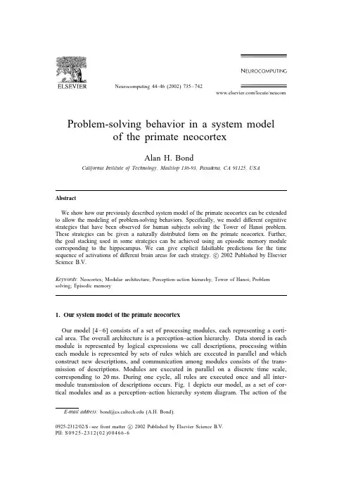
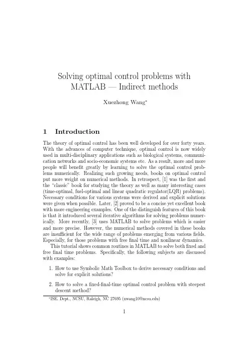
Neurocomputing44–46(2002)735–742/locate/neucomProblem-solving behavior in a system modelof the primate neocortexAlan H.BondCalifornia Institute of Technology,Mailstop136-93,Pasadena,CA91125,USAAbstractWe show how our previously described system model of the primate neocortex can be extended to allow the modeling of problem-solving behaviors.Speciÿcally,we model di erent cognitive strategies that have been observed for human subjects solving the Tower of Hanoi problem. These strategies can be given a naturally distributed form on the primate neocortex.Further, the goal stacking used in some strategies can be achieved using an episodic memory module corresponding to the hippocampus.We can give explicit falsiÿable predictions for the time sequence of activations of di erent brain areas for each strategy.c 2002Published by Elsevier Science B.V.Keywords:Neocortex;Modular architecture;Perception–action hierarchy;Tower of Hanoi;Problem solving;Episodic memory1.Our system model of the primate neocortexOur model[4–6]consists of a set of processing modules,each representing a corti-cal area.The overall architecture is a perception–action hierarchy.Data stored in each module is represented by logical expressions we call descriptions,processing within each module is represented by sets of rules which are executed in parallel and which construct new descriptions,and communication among modules consists of the trans-mission of descriptions.Modules are executed in parallel on a discrete time scale, corresponding to20ms.During one cycle,all rules are executed once and all inter-module transmission of descriptions occurs.Fig.1depicts our model,as a set of cor-tical modules and as a perception–action hierarchy system diagram.The action of theE-mail address:***************.edu(A.H.Bond).0925-2312/02/$-see front matter c 2002Published by Elsevier Science B.V.PII:S0925-2312(02)00466-6736 A.H.Bond/Neurocomputing44–46(2002)735–742Fig.1.Our system model shown in correspondence with the neocortex,and as a perception–action hierarchy.system is to continuously create goals,prioritize goals,and elaborate the highest priority goals into plans,then detailed actions by propagating descriptions down the action hierarchy,resulting in a stream of motor commands.(At the same time,perception of the environment occurs in a ow of descriptions up the perception hierarchy.Perceived descriptions condition plan elaboration,and action descriptions condition perception.) This simple elaboration of stored plans was su cient to allow is to demonstrate simple socially interactive behaviors using a computer realization of our model.A.H.Bond/Neurocomputing44–46(2002)735–7427372.Extending our model to allow solution of the Tower of Hanoi problem2.1.Tower of Hanoi strategiesThe Tower of Hanoi problem is the most studied,and strategies used by human subjects have been captured as production rule systems[9,1].We will consider the two most frequently observed strategies—the perceptual strategy and the goal recursion strategy.In the general case,reported by Anzai and Simon[3],naive subjects start with an initial strategy and learn a sequence of strategies which improve their performance. Our two strategies were observed by Anzai and Simon as part of this learning sequence. Starting from Simon’s formulation[8],we were able to represent these two strategies in our model,as follows:2.2.Working goalsSince goals are created dynamically by the planning activity,we needed to extend our plan module to allow working goals as a description type.This mechanism was much better than trying to use the main goal module.We can limit the number of working goals.This would correspond to using aÿxed size store,corresponding to working memory.The module can thus create working goals and use the current working goals as input to rules.Working goals would be held in dorsal prefrontal areas,either as part of or close to the plan module.Main motivating topgoals are held in the main goal module corresponding to anterior cingulate.2.3.Perceptual tests and mental imageryThe perceptual tests on the external state,i.e.the state of the Tower of Hanoi apparatus,were naturally placed in a separate perception module.This corresponds to Kosslyn’s[7]image store.The main perceptual test needed is to determine whether a proposed move is legal.This involves(a)making a change to a stored perceived representation corresponding to making the proposed move,and(b)making a spatial comparison in this image store to determine whether the disk has been placed on a smaller or a larger one.With these two extensions,we were able to develop a representation of the perceptual strategy,depicted in Fig.2.3.Episodic memory and its use in goal stackingIn order to represent the goal recursion strategy,we need to deal with goal stacking, which is represented by push and pop operations in existing production rule represen-tations.Since we did not believe that a stack with push and pop operations within a module is biologically plausible,we found an equivalent approach using an episodic memory module.738 A.H.Bond/Neurocomputing44–46(2002)735–742Fig.2.Representation of the perceptual strategy on our brain model.This module creates associations among whatever inputs it receives at any given time, and it sends these associations as descriptions to be stored in contributing modules. In general,it will create episodic representations from events occurring in extended temporal intervals;however,in the current case we only needed simple association. In the Tower of Hanoi case,the episode was simply taken to be an association between the current working goal and the previous,parent,working goal.We assume that these two working goals are always stored in working memory and are available to the plan module.The parent forms a context for the working goal.The episode description is formed in the episodic memory module and transmitted to the plan module where it is stored.The creation of episodic representations can proceed in parallel with the problem solving process,and it can occur automatically or be requested by the plan module.Rules in the plan module can retrieve episodic descriptions usingA.H.Bond/Neurocomputing44–46(2002)735–742739the current parent working goal,and can replace the current goal with the current parent,and the current parent with its retrieved parent.Thus the working goal context can be popped.This representation is more general than a stack,since any stored episode could be retrieved,including working goals from episodes further in the past. Such e ects have,in fact,been reported by Van Lehn et al.[10]for human subjects. With this additional extension,we were able to develop a representation of the goal recursion strategy,depicted in Fig.3.Descriptions of episodes are of the form con-text(goal(G),goal context(C)).goal(G)being the current working goal and goal context(C)the current parent working goal.Theÿgure shows a slightly more general version,where episodes are stored both in the episodic memory module and the plan module.This allows episodes that have not yet been transferred to the cortex to be used.We are currently working on extending our model to allow the learning a sequence of strategies as observed by Anzai and Simon.This may result in a di erent representation of these strategies,and di erent performance.740 A.H.Bond/Neurocomputing44–46(2002)735–742during perceptual analysis during movementP MFig.4.Predictions of brain area activation during Tower of Hanoi solving.4.Falsiÿable predictions of brain area activationFor the two strategies,we can now generate detailed predictions of brain area acti-vation sequences that should be observed during the solution of the Tower of Hanoi ing our computer realization,we can generate detailed predictions of activa-tion levels for each time step.Since there are many adjustable parameters and detailed assumptions in the model,it is di cult toÿnd clearly falsiÿable predictions.However, we can also make a simpliÿed and more practical form of prediction by classifying brain states into four types,shown in Fig.4.Let us call these types of states G,E,P and M,respectively.Then,for example,the predicted temporal sequences of brain state types for3disks are:A.H.Bond/Neurocomputing44–46(2002)735–742741For the perceptual strategy:G0;G;E;P;G;E;P;G;E;P;E;M;P;G;E;P;G;E;P;E;M;P;G;E;P;G;E;P;E;M;P;G;E;P;E;M;P;G;E;P;G;E;P;E;M;P;G;E;P;E;M;P;G;E;P;E;M;P;G0:and for the goal recursion strategy:G0;G;E;P;G+;E;P;G+;E;P;E;M;P;G∗;E;P;E;M;P;G∗;E;P;G+;E;P;E;M;P;G∗;E;P;E;M;P;G;E;P;G+;E;P;E;M;P;G∗;E;P;E;M;E;G;E;P;E;M;P;G0: We can generate similar sequences for di erent numbers of disks and di erent strate-gies.The physical moves of disks occur during M steps.The timing is usually about 3:5s per physical move,but the physical move steps probably take longer than the average cognitive step.If a physical move takes1:5s,this would leave about300ms per cognitive step.The perceptual strategy used is an expert strategy where the largest disk is always selected.We assume perfect performance;when wrong moves are made,we need a theory of how mistakes are made,and then predictions can be generated.In the goal recursion strategy,we assume the subject is using perceptual tests for proposed moves, and is not working totally from memory.G indicates the creation of a goal,G+a goal creation and storing an existing goal(push),and G∗the retrieval of a goal(pop). Anderson et al.[2]have shown that pushing a goal takes about2s,although we have taken creation of a goal to not necessarily involve pushing.For us,pushing only occurs when a new goal is created and an existing goal has to be stored.G0is activity relating to the top goal.It should be noted that there is some redundancy in the model,so that,if a mismatch to experiment is found,it would be possible to make some changes to the model to bring it into better correspondence with the data.For example,the assignment of modules to particular brain areas is tentative and may need to be changed.However, there is a limit to the changes that can be made,and mismatches with data could falsify the model in its present form.AcknowledgementsThis work has been partially supported by the National Science Foundation,Informa-tion Technology and Organizations Program managed by Dr.Les Gasser.The author would like to thank Professor Pietro Perona for his support,and Professor Steven Mayo for providing invaluable computer resources.References[1]J.R.Anderson,Rules of the Mind,Lawrence Erlbaum Associates,Hillsdale,NJ,1993.[2]J.R.Anderson,N.Kushmerick,C.Lebiere,The Tower of Hanoi and Goal structures,in:J.R.Anderson(Ed.),Rules of the Mind,Lawrence Erlbaum Associates,Hillsdale,New Jersey,1993,pp.121–142.742 A.H.Bond/Neurocomputing44–46(2002)735–742[3]Y.Anzai,H.A.Simon,The theory of learning by doing,Psychol.Rev.86(1979)124–140.[4]A.H.Bond,A computational architecture for social agents,Proceedings of Intelligent Systems:ASemiotic Perspective,An International Multidisciplinary Conference,National Institute of Standards and Technology,Gaithersburg,Maryland,USA,October20–23,1996.[5]A.H.Bond,A system model of the primate neocortex,Neurocomputing26–27(1999)617–623.[6]A.H.Bond,Describing behavioral states using a system model of the primate brain,Am.J.Primatol.49(1999)315–388.[7]S.Kosslyn,Image and Brain,MIT Press,Cambridge,MA,1994.[8]H.A.Simon,The functional equivalence of problem solving skills,Cognitive Psychol.7(1975)268–288.[9]K.VanLehn,Rule acquisition events in the discovery of problem-solving strategies,Cognitive Sci.15(1991)1–47.[10]K.VanLehn,W.Ball,B.Kowalski,Non-LIFO execution of cognitive procedures,Cognitive Sci.13(1989)415–465.Alan H.Bond was born in England and received a Ph.D.degree in theoretical physics in1966from Imperial College of Science and Technology,University of London.During the period1969–1984,he was on the faculty of the Computer Science Department at Queen Mary College,London University,where he founded and directed the Artiÿcial Intelligence and Robotics Laboratory.Since1996,he has been a Senior Scientist and Lecturer at California Institute of Technology.His main research interest concerns the system modeling of the primate brain.。

使用RunGTAP和WinGEM的操作来介绍GTAP 和GEMPACKKen Pearson and Mark Horridge2005年4月在这份文档中，我们给出了几个你可以操作的动手计算的例子来熟悉RunGTAP和GEMPACK软件的应用。

A部分的案例旨在引导我们如何在GTAP数据库中找到相关的数据。

B部分的案例旨在引导如何运用GTAP展开模拟。

C部分介绍了如何使用RunGTAP软件产生一个新的文本以供使用（即GTAP数据库的聚集）。

D部分假设你已经了解一些有关GEMPACK的知识——它告诉你如何在RunGTAP中调整和运行自己的经济模型。

在E 部分中，我们告知你如何找到更多的有关RunGTAP和GEMPACK的信息，而且提到了一些你更愿去尝试的其他模型而不只是GTAP模型来进行手动计算。

附录A（并未在这个短期课程中使用）给出了在WinGEM下而不是通过RunGTAP进行GTAP模拟的详细指导。

这份文档是为2005年6月在克里特岛举办的GTAP短期课程而设计使用的，它也可以用于课程结束后，与会者结合从本课程中带回去的RunGTAP和GEMPACK软件来使用。

并且由于在下文中提到的某些限制，这篇文档对其他学习使用RunGTAP软件操作的人也很有帮助。

此文档假设你拥有配置如下：(a)RunGTAP的最近版本（版本3.10或者更新，发行于2001年7月或者更晚）(b)带有硬盘的奔腾处理器，至少有32MB的RAM（内存），在Windows95, 98, ME, NT, 2000或者XP环境下运行(c)版本7.0或以上的GEMPACK的源代码或者可执行图像，并且各种有关GTAP的文件都在你的电脑的GTAP目录项下当你阅读此文档时，你可以根据设计的案例来使用RunGTAP和GEMPACK，以便熟悉这些软件的操作，并且更为重要的是熟悉GTAP模型的应用。

RunGTAP是由Mark Horridge 编写的自定义的windows程序，它使得交互式解决全球贸易分析变得更加容易。

Harvard University Economics1123Department of Economics Spring2006Problem Set4–SolutionsGuns&AmmoDue:Thursday9March.1.We will examine the effect of shall on rates of violent crime,murder rates and robberies.To this end,run regressions of the logs of each of these variables on shall(including an intercept)with the robust option.Report the results in a table with a column for each regression and the valuesof the crime rates.Are the effects large in practical terms?Recall that for a dummy variable,the effectˆβ1measures is the difference between the averages of the Y i variable for each of the values for the dummy variable.We see that having a’shall’law is associated with a44%lower violent crime rate,a47%lower murder rate,and a77%lower rate of robberies.These rae all obviously practically significant.If we could really lower these rates by the stated amounts simply by passing such a law(instead of all the other methods of deterrence, which are very costly),we would.(b)Are the effects large statistically?Give a sentence to explain why we care about the statistical significance.The effects are all significant statistically.If we test for the null hypothesis ofˆβ1=0wefind t−statistics of−9or more,clearly lower than the two sided5%bound of−1.96and lower than the two sided1%bound of-2.58.We care about statistical significance because this gives us an idea if the nonzero estimate is likely to be nonzero becauseβ1is truly nonzero and not just because of randomness in the data, which would always lead to an estimate not exactly equal to zero but not really large enough to not be ruled out as just an artifact of the particular sample we obtained.2.Now we will control for a number of variables.First,it is well understood that demographic variables play a role.Many have argued socioeconomic variables also play a part.Most also would at least hope that jail is a deterrent.Run the above regressions but now add the variables incarc_rate, density,pop,pm1029,and avginc to the regression.Report the results in a table as above but now with additional rows.Now the’shall’laws are associated with a36%lower rate of violent crime,a31%lower murder rate and a56%lower rate of robberies.These are still large both statistically and practically.And a little puzzling.Now that we have controlled for many variables,the effect seems still to be of the order that it would be hard to argue against having the laws(but the laws are not in place everywhere).Also,given that murder is more a crime of passion than a rational response,why is the effect so large?(b)Is the difference between the results here and in the results from Question(1)large in a practical sense?All of the coefficients are smaller,suggesting that the omission of the other variables resulted in some omitted variable bias.The effects are quite large–a drop of8%for violent crime,16% for murder rates and21%for robberies.Clearly internal validity is important if we are going to believe the numbers we get from a regression.Here the basic story is the same–the’shall’laws are associated with lower crime rates,however the magnitudes are very susceptible to changes in the specification.3.One omitted variable from the above analysis is differences in laws and law enforcement across states and time.We want to understand how this might affect results to provide more foundation for the interval validity of the results.Write out the omitted variable bias formula.The OVB formula isˆβ1→β1+cov(X1i,u i) var(X1i)(a)How would variations in state law affect u i?Stronger laws would hopefully deter crime,especially crimes that are more rational in nature like roberries,and perhaps violence.In this sense we would expect that stronger laws would be associated with less crime and hence lower values for u i.(b)What do you think the correlation between state laws and the’shall’dummy is?Do you think states that have’shall’laws would be more likely to have stronger laws(i.e.harsher penaltiesetc.)and enforcement than other states?Presumably states where there is a larger’law and order’constituency would have both stronger laws and would be more likely to have’shall’laws.Typically’shall’laws are pushed as using law and order arguments.So we would expect that Cov(X1i,u i)<0where X1i is the dummy variable for shall.(c)If there is a bias inˆβ1(the coefficient on shall),which direction is it?Since Cov(X1i,u i)<0thenˆβ1<β1and hence we expect a negative bias.Notice that this could include the possibility thatβ1=0and that our negative estimates arise because of the ommitted variable.Internal validity is important,remember signs of effects can change and what appear to be effects may simply be picking up the effects of some other variable.Assessing internal validity requires some effort.4.In Australia(where western society was based on transported convicts)it is very difficult to get a permit to carry a concealed weapon.What do the results of the regressions in Question(2) suggest for the differences in crime rates between the US and Australia?Relate your answer to external validity.Since X1i=0is the relevant effect for Australia we expect that,according to these regressions, crime should be much greater on average in Australia than in the US.We have to be careful an remember the other variables in the system,for which Australia might have different values.But in terms of demographics,Australian cities are probably very similar to US ones(both immigrant countries),incomes are not so far apart,incarceration rates are lower but this variable has a pretty small effect.Overall then,we expect higher rates than’shall’states in the US.The opposite is basically true,and there is much reasearch on why.From our perspective then it would seem that external validity is not really justified–there are many unnacounted for differences and hence we might not expect to see the same results.If we could account for the differences we might expect external validity–people are people!。

50
@FOR函数使用不合法
51
编译时LINGO模型生成器的内存不足
52
@IN函数使用不当
53
在电子表格文件中找不到指定的单元范围名称（似乎与出错代码“13”含义类似）
54
读取电子表格文件时出现错误
55
@TEXT函数不能打开文件
56
@TEXT函数读文件时发生错误
57
@TEXT函数读文件时出现了非法输入数据
163
在初始段对变量进行初始化时，给出的参数个数不符
164
模型中输入的符合不符合LINGO的命令规则
165
当前的输出函数不能按集合进行输出
166
不同长度的输出对象无法同时输出到表格型的文件（如数据库和文本文件）
167
在通过Excel进行输入输出时，一次指定了多个单元范围
168
@DUAL,@RANGEU，@RANGED函数不能对文本数据（如集合的成员名）使用，而只能对变量和约束行使用
136
使用@TEXT函数输出时出现错误操作
137
（该项编号目前没有使用）
138
DIVERT (输出重新定向)命令的嵌套次数太多（最多不超过10次嵌套）
139
DIVERT（输出重新定向）命令不能打开指定文件
140
只求原始最优是无法给出敏感性分析信息（可通过“LINGO丨Options”命令对General Solver选项卡中的“Dual Computation”选项进行修改）
146
基本集合的元素名与模型中的变量名重名(当前版本的LINGO种这本来是允许的，但如果通过“LINGO丨Options”命令在”General Solver”选项卡选择“Check for duplicates names in data and model”,则会检查重名，这主要是为了与以前的LINGO版本兼容)

下面只摘录了帖子中的一些主要内容有些地方可能上下文不太连贯完整的讨论请大家根据相应链接去论坛上察看
ABAQUS 常见问题汇总 - 2.0 版
目录 点击小节标题，可以跳到相应的内容（有些 WORD 版本可能需要按住 ctrl 键）
0. ABAQUS 入门资料.......................................................................................................................... 4
6.1 ABAQUS 安装方法 ................................................................................................................. 12 6.2 ABAQUS 显示异常（无法显示栅格、显卡冲突、更改界面颜色）.......................................... 21 6.3 Document 无法搜索................................................................................................................. 21 6.4 磁盘空间不足 ........................................................................................................................... 22 6.5 Linux 系统................................................................................................................................ 22 6.6 死机后恢复模型 ....................................................................................................................... 23

这是我建立的模型，4个钢球1个芯棒1个圆管把芯棒和钢球设为刚体圆管是柔性体，目标是芯棒带动管子向下压，管子和芯棒之间定义摩擦0.2 管子和钢球定义摩擦0.2，钢球用一般约束：xyz位移固定；xyz转动全可。

在芯棒所有面上施加运动副：向下运动、、、网格设置：这是分析设置求解不出来提示信息如下：An error occurred inside the POST PROCESSING module: Invalid or missing result file.The solver engine was unable to converge on a solution for the nonlinear problem as constrained. :Please see the Troubleshooting section of the Help System for more information.The solution failed to solve completely at all time points. Restart points are available to continuethe analysis.The unconverged solution (identified as Substep 999999) is output for analysis debug purposes. Results at this time should not be used for any other purpose.One or more Contact Region(s) contains a friction value larger than .2. To aid in convergence, an unsymmetric solver has been used.Solver pivot warnings have been encountered during the solution. This is usually a result of an ill conditioned matrix possibly due to unreasonable material properties, an under constrained model, or contact related issues. Check results carefully.Contact status has experienced an abrupt change. Check results carefully for possible contact separation.Although the solution failed to solve completely at all time points, partial results at some points have been able to be solved. Refer to Troubleshooting in the Help System for more details.翻译版：无效或缺失的结果文件：后处理模块内部发生错误。

d
b
c
e
Copyright 2005 MSC.Software Corporation 5
Step2:导入模型
a h i
b
c
从Parasolid文件导入模型。 a. File / Import… b. 在Source: 设定为 Parasolid xmt 。 c. 点击Parasolid xmt Options… 按钮。 d. 点击Model Units… 按钮。 e. 设定Model Unit Override 为 1.0 (Meters) 。 f. 点击OK 。 g. 点击OK 。 h. 选择Simple-conrod.xmt 。 i. 点击-Apply- 。
a
b f d c i
e
g
Copyright 2005 MSC.Software Corporation 15
h
Step6:定义材料特性
a
定义模型的材料特性。 a. b. c. d. 选择Material | Create | Isotropic | Manual Input 。 在“Material Name” 中输入Steel 。 点击Input Properties… 按钮。 在“Elastic Modulus” 中输入 2.1e11 在“Poisson Ratio” 中输入 0.3 在“Density” 中输入 7.8e3 在“Structural Damping Coeff”中输入 0.1 。 点击OK 。 点击Apply 。
d b
c
e
a
Copyright 2005 MSC.Software Corporation 19
Step8:分析设定
a. b.
点击Solution Parameters… 。 点击ADAMS Preparation… 。