Integrated planning and control for convex-bodied nonholonomic systems using local feedback
- 格式:pdf
- 大小:1.69 MB
- 文档页数:50

Jobscope,the most comprehensive job costing and integrated business information system for your order-driven company, balances critical requirements, function,and technology while offering the comfort and confidence necessary to overcome your unique business challenges.®Production Planning and Control• Provides for purchasing and tracking longlead-time items prior to engineering completion.• Shows material availability prior tocommitting work to the shop• Provides the capability to release pre-engineered lower level items prior to releasing the overall assembly.• Creates multiple work orders for a complex assembly in a single process.• Maintains complex work order dependencies and schedules the work orders accordingly.•Provides a selection of both forward scheduling from a start date or backward scheduling from a completion date.• Ensures that work may be changed from “make” to “buy” either before or after the work begins.•Allows employees to log on and off work, perform QA inspections, and view electronic documents and drawings.• Automatically updates the shop schedule and job cost when employees log on/off the system.•Displays graphical views of work order and shop status.Project ManagementAfter the Project Manager defines the work in Microsoft Project, the Engineering and Production Planning and Control departments may link the engineering releases and production work orders to the project tasks. This allows engineering release and production work order status to be reported by project task. In addition, the project manager may change project task dates and send the new date requirements to the shop scheduling system.Engineering ReleasesProduction Planning and Control receives theEngineering information in the form of engineering releases. The engineering releases track the work through the engineering and production planningprocess. As each department completes its work on an engineering release, the department electronically sends the work to the next department, allowing tracking of where the work is, how long it stayed in eachdepartment, and how much backlog each department has. Production Planning and Control turns thesereleases into work orders and purchasing requirements.The engineering release contains engineering release line items, or lines, which identify the drawings, bills of material, and other data that are being released. Some of the release line items, or lines, require routings to be created. This work is done in Production Planning and Control.Engineering release lines may release drawings and bills of material for items, which are part of larger assemblies not yet released. Jobscope’s Production Planning and Control subsystem explodes eachengineering release line into planning work orders and shows like items previously released on the job. The production planner may then decide how to disposition these lower level items.The production planner may disposition a planning work order or group of planning work orders in a number of different ways.• Create shop work orders from the planning work order(s)• Purchase the item or items on the planning work order(s)• Designate that the planning work order(s) is covered on another engineering release• Designate that the planning work order(s) will be superseded by a another release (such as design engineering errors)• Substitute an alternate item• Combine the planning work order with an existing work order The results of these dispositions are routedautomatically to the Shop Floor, Purchasing, or back to Engineering.Procuring MaterialsThe project may require long lead-time materials, which must be ordered immediately after the order is received.These items may be ordered immediately and tracked to avoid duplicating the orders when the engineering is completed. Items, which are normally produced in thepurchasing.Work OrdersA large, complex, overall assembly requiring extensive engineering may have lower level subassemblies, which are already engineered. These lower levelsubassemblies may be released for production prior to completion of the engineering for the overall assembly.When the engineering for the overall assembly iscomplete and ready for production, the subassemblies released earlier are identified to prevent duplication.Dependencies between work orders (what is used on what) are automatically created when the work orders are created. These dependencies may quickly bechanged in the event that the work is to be performed in a different sequence that the engineering designwould indicate. The shop floor scheduling system takes these dependencies into account.Production SchedulingThis screen shows the full, multi-level BOM.This screen tracks engineering releases.This screen shows the complete work order listing.Schedule ProductionWork may be scheduled through Online Scheduling(accessed through the Route/Schedule button on the Job Line Items screen) or through Schedule Production.Schedule Production allows you to choose theoperations that are to be scheduled in several ways; for example, you may schedule all in-completed work, all work that has not yet been scheduled, work associated with specified releases, and work that has beendisplaced by other operations with higher priorities. When production is scheduled, the system determines the time required for a block of work and looks at the existing “holes” in the schedule of the appropriate work center. If, given the constraints assigned by finitepercentages and priorities, the “hole” is large enough to accommodate the work, the production is scheduled; if not, then the system continues to look for a suitable time to schedule work.The Adjust Schedule screen allows you to adjust the schedulefor an entire release or an end work order.The Schedule Production screens allow you to globally schedule or reschedule production.Schedule BoardThe Scheduling Board is used to display schedules and projects.ChangesChanges due to customer requirements, shop load,installation delays, and many other causes, can upset the schedule. The work orders may be changed, or cancelled and purchased outside, or cancelledaltogether. Additional work orders may be quickly created to handle the change, and rework work orders quickly created to handle QA rejects.Bringing The System To The Shop FloorThis screen allows the JOBSCOPE Production Scheduleto be exported to Microsoft Project.system, and employee records. QA inspectors may view the inspection instructions and requirements for tools,fixtures, and equipment. The inspectors may report inspection results on these workstations. Both direct employees and inspectors may view the electronic documents linked to their work on these same workstations.Office and Shop Floor StatusThe status of work orders, materials, and work center backlog may be viewed with graphical aids. Behind schedule work is highlighted to draw attention to scheduling problems. Material availability is color coded to point out material problems. Status symbols show where the work is in the engineering process.or only for the cumulative number entered.This screen displays the JOBSCOPE Production Schedule in Microsoft Project.The legend defines the colors and symbols in the BOM.This screen allows you to view the status of a specific job.®Jobscope Corporation355 Woodruff Road · Suite 406 Greenville · South Carolina29607800.443.5794864.234.4852 (fax)。
城市规划与管理专业英语English City Planning and Management光明城市The radiant city翻译成员:111855128熊能111855125汤豪111855108程志111855104陈世峰111855107谌博111855133张菂111855119李胜鸾111855122栾楠The Radiant City光明城市The Radiant City retained the most important principle of the Contemporary City:the juxtaposition of a collective realm of order and administration with an individualistic realm of family life and participation.光明城理论保持了现代城市构想中最重要的原则:让充斥着秩序和管理的集体王国与以家庭生活和分享为特征的个人空间完美地结合。
This juxtaposition became the key to Le Corbusier’s attempt to resolve the syndicalist dilemma of authority and participation.Both elements of the doctrine receive intense expression in their respective spheres.Harmony is in the structure of the whole city and in the complete life of its citizens.这种结合成了柯布西耶试图解决工团主义者自身权威与参与的两难境地的关键。
这两个要素都在它们各自的领域收获了强烈的表现效果。
和谐存在于整个城市的结构体系中以及城市公民整个生活中。
工程职称英语试题及答案一、选择题(每题1分,共10分)1. The term "engineering" refers to:A. A type of professionB. A specific disciplineC. A method of constructionD. A type of technology答案:A2. Which of the following is not a characteristic of engineering?A. SystematicB. PracticalC. CreativeD. Static答案:D3. The basic elements of engineering include:A. Materials, energy, and informationB. Money, manpower, and materialsC. Information, technology, and moneyD. Energy, manpower, and technology答案:A4. The primary goal of engineering is to:A. Solve practical problemsB. Pursue scientific truthC. Achieve artistic expressionD. Maximize economic benefits答案:A5. The role of engineering in society includes:A. Enhancing the quality of lifeB. Promoting social progressC. Protecting the environmentD. All of the above答案:D6. The engineering design process generally includes the following stages except:A. Problem identificationB. Conceptual designC. FabricationD. Market research答案:D7. Which of the following is not a common method of engineering analysis?A. Mathematical modelingB. Experimental researchC. Literature reviewD. Computer simulation答案:C8. In engineering, the concept of "sustainability" refers to:A. Economic sustainabilityB. Environmental sustainabilityC. Social sustainabilityD. All of the above答案:D9. The "Internet of Things" (IoT) is related to engineering because it:A. Enhances communication capabilitiesB. Facilitates remote monitoring and controlC. Reduces the need for human laborD. B and C only答案:B10. The acronym "CAD" stands for:A. Computer-Aided DesignB. Computer-Aided DraftingC. Computer-Aided DevelopmentD. Computer-Aided Diagnostics答案:A二、填空题(每空1分,共10分)11. The ________ of an engineering project refers to its ability to meet the needs of the users.答案:functionality12. In engineering, the term "feasibility study" is used to evaluate the ________ and practicality of a project.答案:viability13. The process of converting raw materials into finished products is known as ________.答案:manufacturing14. The use of renewable energy sources is an example of engineering efforts to achieve ________.答案:sustainability15. A ________ is a tool that engineers use to createdetailed drawings of their designs.答案:CAD software16. The ________ of a structure refers to its ability to withstand loads without breaking or deforming excessively.答案:stability17. In the context of engineering, "innovation" often involves the development of new ________ or processes.答案:products18. The ________ of a project refers to the total cost of all the resources required to complete it.答案:budget19. Environmental impact assessments are conducted to evaluate the potential ________ of a project on the naturalsurroundings.答案:effects20. The term "mechatronics" combines elements of mechanical engineering, electronics, and ________.答案:computer engineering三、简答题(每题5分,共20分)21. What are the key factors that engineers consider when designing a bridge?答案:Key factors include the bridge's intended load capacity, the materials to be used, the environmental conditions it will be subjected to, and the overall cost of construction.22. Explain the difference between "prototype" and "final product" in the context of engineering.答案:A prototype is an early sample or model of aproject used to test concepts and processes. The finalproduct is the completed, polished version that is ready for use or distribution.23. What is the significance of "risk assessment" in engineering projects?答案:Risk assessment is significant as it helps identify potential hazards and assess their likelihood and impact.This allows engineers to take preventive measures and ensure the safety and success of the project.24. Describe the role of "project management" in engineering.答案:Project management in engineering involves planning,organizing, and controlling resources to achieve specific project goals. It includes scheduling, budgeting, and coordinating the efforts of the team to ensure timely completion and adherence to quality standards.四、论述题。
项目总体规划及流程的英语英文回答:As a project manager, it is crucial to have a well-defined overall plan and process in place to ensure the successful execution of a project. The overall planning and process involve several key steps and considerations.Firstly, it is essential to clearly define the project objectives and goals. This includes understanding the desired outcomes, deliverables, and the overall purpose of the project. For example, if the project is to develop a new software application, the objective could be to create a user-friendly and efficient system that meets thespecific needs of the target users.Once the objectives are defined, the next step is to identify the project scope. This involves determining the boundaries and limitations of the project, including what is included and excluded. For instance, if the softwareapplication project scope includes only the development phase and not the implementation and maintenance phases, it is important to clearly communicate this to all stakeholders.After defining the objectives and scope, the project manager needs to create a detailed project plan. This plan outlines the tasks, timelines, resources, and dependencies required to complete the project. It is important to break down the project into smaller, manageable tasks and assign responsibilities to team members. For example, if the software application project plan includes tasks like requirements gathering, design, coding, and testing, the project manager should allocate specific timeframes and resources for each task.Once the project plan is in place, the project manager needs to monitor and control the project progress. This involves tracking the actual progress against the planned schedule, identifying any deviations or risks, and taking corrective actions if necessary. For instance, if the coding phase of the software application project is behindschedule, the project manager may need to allocate additional resources or adjust the timeline to ensure timely completion.Furthermore, effective communication is vital throughout the project. The project manager shouldregularly communicate with all stakeholders, including team members, clients, and senior management. This helps in maintaining transparency, managing expectations, and addressing any concerns or issues that may arise. For example, if there is a change in the project requirements, the project manager should promptly communicate this to the team and discuss the necessary adjustments.In conclusion, the overall planning and process of a project involve defining objectives, identifying scope, creating a detailed project plan, monitoring progress, and maintaining effective communication. By following these steps and considering the specific requirements of the project, a project manager can increase the chances of successful project execution.中文回答:作为一个项目经理,在项目的成功执行过程中,拥有明确的总体规划和流程是至关重要的。
英文回答:The responsibilities and role of the Integrated Systems Project Management Engineer in chapter II of the third edition of the Academy of Systems Integrated Project Management Engineers are an integral part of project management。
Work elements such as project planning, implementation and closure address related concepts and methods such as project management knowledge systems, integration management, scope management and time management。
Attention also needs to be given to detailed explanations in the areas of cost management, quality management, human resources management andmunication management。
By learning the content of this chapter, the reader will gain aprehensive understanding of the work responsibilities and project management fundamentals of the integrated project management engineers of the system and will provide a solid basis for future practical work to better serve the routes,guidelines and policies of the party and the country。
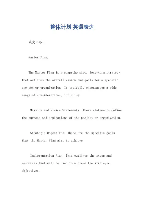
整体计划英语表达英文回答:Master Plan.The Master Plan is a comprehensive, long-term strategy that outlines the overall vision and goals for a specific project or organization. It typically encompasses a wide range of considerations, including:Mission and Vision Statements: These statements define the purpose and aspirations of the project or organization.Strategic Objectives: These are the specific goalsthat the Master Plan aims to achieve.Implementation Plan: This outlines the steps and resources that will be used to achieve the strategic objectives.Monitoring and Evaluation Plan: This establishes mechanisms for tracking progress and making adjustments as necessary.The Master Plan serves as a roadmap for decision-making and resource allocation throughout the life of the project or organization. It provides a clear understanding of the intended direction and facilitates coordination among stakeholders.Components of a Master Plan.A comprehensive Master Plan typically includes the following components:Executive Summary: A brief overview of the plan's key points.Background and Context: Information about the organization, project, or issue that the plan addresses.Mission and Vision Statements: Clear and concisestatements that define the purpose and aspirations of the project or organization.Strategic Objectives: Specific, measurable, achievable, relevant, and time-bound (SMART) goals.Implementation Plan: A detailed outline of the steps and resources that will be used to achieve the strategic objectives. This may include timelines, budgets, and personnel assignments.Monitoring and Evaluation Plan: A framework fortracking progress, identifying areas for improvement, and making adjustments as needed. This may include performance indicators, data collection methods, and reporting mechanisms.Appendices: Supporting documents, such as financial projections, stakeholder lists, or technical specifications.Importance of the Master Plan.A well-developed Master Plan is essential for ensuring the success of a project or organization. It provides a clear roadmap for decision-making, facilitates coordination among stakeholders, and enables effective monitoring and evaluation.Clarity and Direction: The Master Plan provides a shared understanding of the project's or organization's goals and objectives. This clarity helps to align efforts and ensure that everyone is working towards the same outcomes.Resource Allocation: The Master Plan helps to determine the resources that are needed to achieve the strategic objectives. This information can be used to develop realistic budgets and secure funding.Stakeholder Coordination: The Master Plan outlines the roles and responsibilities of different stakeholders. This helps to avoid duplication of effort and ensure that everyone is contributing effectively.Monitoring and Evaluation: The Master Plan establishes a framework for tracking progress and making adjustments as needed. This allows for early detection of potential risks and opportunities.Developing a Master Plan.Developing a Master Plan is an iterative process that typically involves the following steps:1. Stakeholder Engagement: Identify and engage with all stakeholders, including project team members, management, clients, and the community.2. Needs Assessment: Gather information and conduct analysis to identify the needs and challenges that the Master Plan will address.3. Goal Setting: Develop clear and achievable strategic objectives for the project or organization.4. Implementation Planning: Outline the specific steps,resources, and timeline that will be used to achieve the strategic objectives.5. Monitoring and Evaluation Planning: Establish mechanisms for tracking progress, identifying areas for improvement, and making adjustments as needed.6. Documentation and Communication: Develop a comprehensive Master Plan document and communicate it effectively to all stakeholders.Conclusion.The Master Plan is a critical tool for project and organizational success. It provides a roadmap for decision-making, resource allocation, stakeholder coordination, and monitoring and evaluation. By following a well-developed Master Plan, project and organizational leaders can increase their chances of achieving their goals and objectives.中文回答:总体计划。
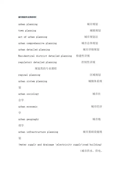
城市规划专业英语词汇unban planning 城市规划town planning 城镇规划act of urban planning 城市规划法urban comprehensive planning 城市总体规划urban detailed planning 城市详细规划Residentiral district detailed planning 修建性详规regulatory detailed planning 控制性详规规划类的专业课程reginal planning 区域规划urban system planning 城镇体系规划urban sociology 城市社会学urban economic 城市经济学urban geograghy 城市地理学urban infrastructure planning 城市基础设施规划(water supply and drainage \electricity supply\road building)(城市供水、供电、道路修建)urban road system and transportation planning 城市道路系统和交通规划urban road cross-section 城市道路横断面RS=remote sensing 遥感Gardening==Landscape architecture 园林=营造景观学Urban landscape planning and design 城市景观规划和设计Urban green space system planning 城市绿地系统规划Urban design 城市设计Land-use planning 土地利用规划The cultural and historic planning 历史文化名城Protection planning 保护规划Urbanization 城市化Suburbanization 郊区化Public participation 公众参与Sustainable development(sustainability) 可持续性发展(可持续性)Over-all urban layout 城市整体布局Pedestrian crossing 人行横道Human scale 人体尺寸(sculpture fountain tea bar) (雕塑、喷泉、茶吧)Traffic and parking 交通与停车Landscape node 景观节点Brief history of urban planningArchaeological 考古学的Habitat 住处Aesthetics 美学Geometrical 几何学的Moat 护城河Vehicles 车辆,交通工具,mechanization 机械化merchant-trader 商人阶级urban elements 城市要素plazas 广场malls 林荫道The city and region Adaptable 适应性强的Organic entity 有机体Department stores 百货商店Opera 歌剧院Symphony 交响乐团Cathedrals 教堂Density 密度CapacityCirculation 循环Elimination of water 水处理措施In three dimensional form 三维的Condemn 谴责Rural area 农村地区Regional planning agencies 区域规划机构Service-oriented 以服务为宗旨的Frame of reference 参考标准Distribute 分类Water area 水域Alteration 变更Inhabitants 居民Motorway 高速公路Update 改造论文写作Abstract 摘要Key words 关键词Reference 参考资料Urban problemDimension 大小Descendant 子孙,后代Luxury 奢侈Dwelling 住所Edifices 建筑群<Athens Charter>雅典宪章Residence 居住Employment 工作Recreation 休憩Transportation交通Swallow 吞咽,燕子Urban fringes 城市边缘Anti- 前缀,反对……的;如:antinuclear反核的 anticlockwise 逆时针的Pro- 前缀,支持,同意……的;如:pro-American 亲美的pro-education重教育的Grant 助学金,基金Sewage 污水Sewer 污水管Sewage treatment plant 污水处理厂Brain drain 人才流失Drainage area 汇水面积Traffic flow 交通量Traffic concentration 交通密度Traffic control 交通管制Traffic bottleneck 交通瓶颈地段Traffic island 交通岛(转盘)Traffic point city 交通枢纽城市Train-make-up 编组站Urban redevelopment 旧城改造Urban revitalization 城市复苏Urban FunctionUrban fabric 城市结构Urban form 城市形体Warehouse 仓库Material processing center 原料加工中心Religious edifices 宗教建筑Correctional institution 教养院Transportation interface 交通分界面CBD=central business district 城市中心商业区Public agencies of parking 停车公共管理机构Energy conservation 节能Individual building 单一建筑Mega-structures 大型建筑Mega- 大,百万,强Megalopolis 特大城市Megaton 百万吨R residence 居住用地黄色C commercial 商业用地红色M manufacture 工业用地紫褐色W warehouse 仓储用地紫色T transportation 交通用地蓝灰色S square 道路广场用地留白处理U utilities 市政公共设施用地接近蓝灰色G green space 绿地绿色P particular 特殊用地E 水域及其他用地(除E外,其他合为城市建设用地)Corporate 公司的,法人的Corporation 公司企业Accessibility 可达性;易接近Service radius 服务半径Urban landscapeTopography 地形图Well-matched 相匹配Ill-matchedVisual landscape 视觉景观Visual environment 视觉环境Visual landscape capacity 视觉景观容量Tour industry 旅游业Service industry 服务业Relief road 辅助道路Rural population 城镇居民Roofline 屋顶轮廓线风景园林四大要素:landscape plantarchitecture/buildingtopographywaterUrban designNature reserve 自然保护区Civic enterprise 市政企业Artery 动脉,干道,大道Land developer 土地开发商Broad thorough-fare 主干道Water supply and drainageA water supply for a town 城市给水系统Storage reservoir 水库,蓄水库Distribution reservoir 水库,配水库Distribution pipes 配水管网Water engineer 给水工程师Distribution system 配水系统Catchment area 汇水面积Open channel 明渠Sewerage system 污水系统,排污体制Separate 分流制Combined 合流制Rainfall 降水Domestic waste 生活污水Industrical waste 工业污水Stream flow 河流流量Runoff 径流Treatment plant 处理厂Sub-main 次干管Branch sewer 支管City water department 城市供水部门UrbanizationSpatial structure 空间转移Labor force 劳动力Renewable 可再生*Biosphere 生物圈Planned citiesBlueprints 蓝图License 执照,许可证Minerals 矿物Hydroelectric power source 水利资源Monuments 纪念物High-rise apartment 高层建筑物Lawn 草地Pavement 人行道Sidewalk 人行道Winding street 曲折的路A view of VeniceMetropolis 都市Construction work 市政建设Slums 平民窟Alleys 大街小巷Populate 居住Gothic 哥特式Renaissance 文艺复兴式Baroque 巴洛克式land allocation拨地Land and Building Advisory Committee [LBAC]土地及建设谘询委员会land assembly汇集土地;征集土地land bank土地储备;土地备用区land classification土地分类;土地分等land cost土地成本land development土地发展Land Development Corporation [LDC]土地发展公司〔土发公司〕Land Development Corporation Managing Board土地发展公司管理局Land Development Corporation Ordinance [Cap. 15]《土地发展公司条例》〔第15章〕land disposal批地land disposal programme批地计划land drainage and flood path system土地排水及防洪道系统Land Drainage Ordinance [Cap. 446]《土地排水条例》〔第446章〕land extensive industry广占土地的工业land form地形land formation土地平整;土地开拓land freight transport陆上货运land grant批地land holding consolidation土地业权收集land index土地指数Land Information System [LIS]土地信息系统land intensive industry土地集约工业land law土地法land lease批地契约;土地契约land levelling土地平整land management土地管理land owner土地拥有人;土地业权人;地主land ownership土地拥有权;土地业权land policy土地政策land premium地价;土地补价land production增辟土地land readjustment土地规划调整land reclamation填海辟地Land Record土地记录land registration土地注册Land Registration Ordinance [Cap. 128]《土地注册条例》〔第128章〕land resource土地资源land resumption收回土地land revenue土地收益land right土地权land sales programme售地计划land status土地类别;土地性质Land Sub-committee [Land and Building Advisory Committee]土地小组委员会〔土地及建设谘询委员会〕land supply土地供应land surveying土地测量land tenure土地年期;土地批租期;土地租用权;土地保有权land transaction土地交易land transport陆上运输land use土地用途land use classification土地用途分类land use control土地用途管制land use performance土地用途效能land use plan土地用途图则;土地用途计划land use survey土地用途调查Land Use Transport Optimization Model [LUTO]土地及运输最佳配合模式land use zoning土地用途地带;土地用途地带区划land valuation土地估价land value地价landed property地产landfill堆填区;垃圾堆填区landlord业主;地主;房东landmark地界标志;地志Lands Tribunal土地审裁处Lands Tribunal Ordinance [Cap. 17]《土地审裁处条例》〔第17章〕landscape景观;风景;园景landscape appraisal景观评估landscape architecture景观建筑学;园林建筑学;园景设计学landscape buffer园景缓冲区landscape conservation area景观保育区landscape mounding景观土丘landscape plan景观设计图landscape planning景观规划landscape protection area景观保护区;风景保护区landscape reinstatement景观重整;园景修复landscape strategy景观策略landscape value景观价值landscaped area景观美化地方;园景美化地方landscaping景观美化;环境美化landscaping proposal美化环境计划书landside非禁区〔机场〕landslide山泥倾泻landslip山泥倾泻lane行车线;车道;小巷Lantau Link青屿干线Lantau Port and Western Harbour Development Studies大屿山港口及西部海港发展研究Lantau Port and Western Harbour Development Studies Final Rep ort--Executive Summary《大屿山港口及西部海港发展研究最后报告──摘要》Lantau Port Development--Stage 1, Container Terminals 10 and11 Ancillary Works (Design) Study大屿山港口发展──第一期工程十号及十一号货柜码头附属工程(设计)研究Lantau Port Development--Stage 1, Container Terminals 10 and 11 (Preliminary Design) Study大屿山港口发展──第一期工程十号及十一号货柜码头(初步设计)研究large site reduction factor大型地盘折减因素latrine厕所launderette自助洗衣店laundry洗衣店;洗衣房lay-by避车处;路旁停车处;停车湾layout布局设计;设计;规划图layout area蓝图区;详细规划区layout plan发展蓝图;详细蓝图leachate treatment works渗滤污水处理厂lead time筹建时间lease批约;租约;租契;契约lease conditions批约条件;契约条件;批地条件;租赁条件;批约条款lease enforcement强制执行批约条款lease modification契约修订lease modification premium契约修订补价lease restriction契约限制lease term契约年期;租赁年期leased area批租地区leased land已批租土地leasehold按租约而持有业权legend图例lessee承租人;租户lessor批租人;出租人Letter "A"甲种换地权益书Letter "B"乙种换地权益书letter of intent意向书letter of modification建筑牌照规约修订书;契约修订书;批地条款修订书level crossing平交道口;铁路公路交叉点level of confidence置信程度level of significance显著水平library图书馆lifeguard tower救生员了望塔light industrial area轻工业区light industry轻工业Light Rail Scheme reserve轻便铁路计划专用范围Light Rail System轻便铁路系统Light Rail Transit [LRT]轻便铁路〔轻铁〕Light Rail Transit reserve轻便铁路专用范围Light Rail Transit terminus轻便铁路总站light traffic交通稀疏light well天井light-controlled junction灯号控制的路口lighter趸船;驳船limited access road限制出入的通道;限制出入的通路linear analysis图线分析linear block相连长形大厦linear city带形城市linear correlation线性相关linear development线状发展linear programming线性规划linear regression线性回归link连接部分;连接线link road连接路linked development相关发展linked project相关计划;相关工程linked signal system联动式交通灯系统linked site相关地盘livability适居程度livestock upgrading area禽畜业发展改善区livestock waste treatment禽畜废物处理living density居住密度living quarters住所living quarters frame屋宇单位记录库living quarters size住所面积load bearing负荷;承重load factor负荷率loading/unloading area上落客货区loading/unloading bay上落客货处loading/unloading facility上落客货设施local access road区内通道local centre地区中心;乡区中心local development value地区性发展价值local distributor地区干路local open space邻舍休憩用地local plan地区规划图local public works地区性小工程;乡村工程local traffic地区交通;区内交通locality地区;地点location plan位置图location theory区位论;位置理论locational requirement位置需求lodging house旅馆Long Term Housing Strategy长远房屋策略Long Term Road Study长期道路研究longitudinal profile纵断面图longitudinal section纵剖面;纵切面long-term development长远发展long-term planning长远规划lookout area观景区lookout pavilion观景亭lookout point观景处;观景台loop road回旋路;环路lorry and car parking货车及汽车停放处lot地段lot amalgamation地段合并lot boundary地段界线lot number地段编号lot section地段分段low tide低潮low-density residential development低密度住宅发展lower catchment area下段集水区lowland低地lowland rural area低地乡郊地区low-rise building矮楼宇;层数较少的楼宇low-rise development低层建筑lump sum contract整笔付款合约MMa Wan Feasibility Study马湾发展可行性研究macro-analysis宏观分析magistracy裁判法院main elevation主立视面maintenance depot维修站maisonette复式住宅major business centre主要商业中心major road主要道路mall商场;购物中心;广场;林荫道mangrove area红树林地区manhole沙井;探井man-land ratio人地比率manufacturing industry制造业map地图;图mapping survey地图制作测量mariculture海鱼养殖marina船只停泊处marine activity海事活动marine borrow area海上采泥区marine dumping area海上倾倒物料区marine engine workshop轮机工场Marine Fill and Disposal Strategy海上填料与倾卸策略marine fish culture海鱼养殖marine fuel depot船舶燃油库marine fuelling station船舶加油站marine mud海岸淤泥marine park海岸公园Marine Parks Ordinance [Cap. 476]《海岸公园条例》〔第476章〕marine research centre海洋研究中心marine reserve海岸保护区marine services support area海事服务后勤用地marine spoil ground海上废土场marine traffic海上交通marine-oriented industrial use与海事有关的工业用途marine-related facility与海事有关的设施marine-related repair workshop与海事有关的修理工场Mark I block [public housing]第一型大厦〔公屋〕Mark II block [public housing]第二型大厦〔公屋〕Mark III block [public housing]第三型大厦〔公屋〕Mark IV block [public housing]第四型大厦〔公屋〕Mark V block [public housing]第五型大厦〔公屋〕Mark VI block [public housing]第六型大厦〔公屋〕market街市;市场;市集market garden果菜园market gardening种植商品果菜market rent市值租金;市面租金market stall街市档位market town墟镇;市镇market value市价;市值marsh沼泽marshalling yard调车场;编组场mart市场;贸易中心;交易会mass transit line集体运输路线Mass Transit Railway [MTR]地下铁路〔地铁〕Mass Transit Railway concourse地下铁路车站大堂Mass Transit Railway depot地下铁路厂房Mass Transit Railway (Land Resumption and Related Provisions) Ordinance [Cap. 276]《地下铁路(收回土地及有关规定)条例》〔第276章〕Mass Transit Railway Modified Initial System地下铁路修正早期系统Mass Transit Railway tunnel地下铁路隧道Mass Transit Railway works area地下铁路工程区mass transit system集体运输系统Mass Transit vent shaft地下铁路通风塔Mass Transit vent shaft and other structures above ground lev el other than entrances地下铁路通风塔及高出路面的其他构筑物(入口除外)massage establishment按摩院master landscape plan园景设计总图master layout plan总纲发展蓝图master plan总纲规划;总纲图master scheme总纲计划material change of use实质改变用途material considerations实质考虑因素matrix矩阵matshed theatre戏棚mature tree成长树木;成材树mausoleum多层式陵墓maxicab/public light bus stand专线小巴/公共小型巴士站maximum attainable level可达到的最高水平maximum building height最高建筑物高度maximum permissible level准许的最高限度maximum population capacity最多可容纳人口数目meadow草场mean平均数mean formation level地基平均水平线;平均地基面mean household size平均家庭人数;平均住户人数mechanism机制;制度median中位数median income收入中位数medical laboratory医疗化验室medium density中等密度megalopolis大都会memorial park纪念公园memorial stone纪念碑mental hospital精神病院merging intersection汇点merging lane合流车道merging traffic合流交通meter room电表房methane沼气metre above Principal Datum [mPd]主水平基准以上……米metro area都会区Metro District Planning Division [Planning Department]都会区规划部〔规划署〕Metro Group Section [Planning Department]都会组〔规划署〕Metro Planning Committee [MPC] [Town Planning Board]都会计划小组委员会〔城市规划委员会〕Metroplan都会计划Metroplan Study都会计划研究metropolis都会metropolitan area都会区mezzanine阁楼micro-analysis微观分析mid-stream operation中流作业migration迁移military area军事地区military camp军营military land军事用地military use军事用途mine矿场minibus小型巴士mining and quarrying采矿及采石业mini-soccer pitch小型足球场minor road次级道路minor supply gathering ground小水量集水区mitigation measure纾缓措施mixed rental/HOS estate租住公屋及居屋混合式屋mixed use building混合用途楼宇mixed woodland混合林地moat护城河;城壕mobile clinic流动诊所mobile labour流动劳动力mobility流动性mock-up flat示范单位modal split各类交通工具乘客率分析mode方式;模式;众数〔统计学〕model模式;模型model flat示范单位modification修订;更改modification of lease修订契约modification of lease conditions契约条件修订modular market标准型街市monastery寺院monastery belt寺院地带Monetized Letter "B"币值化的乙种换地权益书money exchange外币兑换店monitoring监察monorail单轨铁路monument纪念性建筑物;遗址;古mooring buoy系泊浮筒;系船浮泡moratorium延期履行;延期履行权;冻结;冻结期mortality rate死亡率mortuary殓房mosque清真寺motel时租旅店;汽车酒店motor vehicle assembly plant汽车装配厂motor vehicle showroom汽车陈列室motorway高速公路moulding装饰线条mud disposal area弃土倾卸场;卸泥场mudflats泥滩multi-disciplinary涉及多种学科multi-leg intersection多线道路交汇点multi-level junction多层路口multiple ownership共有业权multiple regression analysis复回归分析multi-purpose building多用途楼宇multi-purpose terminal多用途码头multi-service centre for the elderly老人服务中心multi-storey block多层大厦multi-storey building多层大厦multi-storey car park多层停车场multi-storey car/lorry park私家车/货车多层停车场multivariate analysis多元变量分析museum博物馆music bowl露天音乐场music hall音乐厅。
项目计划进度控制与资源管理(Project plan, schedule controland resource management)Project plan, schedule control and resource managementWith the further deepening of the implementation of project management and construction enterprise reform, not to adjust the management mechanism to adapt to the management system and the internal operation of the market of the poor to various levels of management, enterprise project management as the main line, to establish the management system of construction management and operation layer two layer separation, the rational allocation of production factors, high efficiency the operation of the project, make full use of resources, resources, organic combination of progress in the implementation of schedule control is the key to achieve the project goals.First, the implementation of integrated control of schedule resources, the realization of the project as the source of profits, is to strengthen management and explore the market needsThe realization of the whole target of project management must be controlled by the organic, integrated and timely process control of all construction management under the serious and scientific plan control and reasonable and effective resources investment. Time, cost, quality and safety of the four control in the implementation of the project, cost perspective, as the cost center of the project department, in order to implement the cost control based on very fruitful, will it be possible to create a Everfount profit source, make it possible forenterprises to survive and continue to develop.The total cost of the project during the construction stage occurred, mainly focus on the organization and management of formal project, direct purpose and this stage invested a lot of manpower and material resources to meet the owners recognized each stage progress goals, and achieve the business income to make up for the process of investment, eventually achieve the overall project objectives and project total profit value. The construction schedule objectives through the implementation and control of stage schedule, all kinds of people, financial and material resources around the implementation schedule synchronization input, coordination and support, and implement under integrated control.Thus, planning system should further enrich and perfect and improve, especially the management of the progress of the project construction must be strengthened, in order to adapt to the management, extension of the market requirements, the construction schedule management plan with other resources combine to achieve the best effect of comprehensive control. And enterprises to explore the market closely, more contract construction tasks, and better do the existing works. In the face of the grim situation of limited construction market and numerous competitors, enterprises to adapt to market and market development, seize market opportunities at the same time, only the work in cooperation, properly organized, scientific and orderly, solid and effective basis, to sensitive information, the decision is correct, the implementation of effective and correct aircraft, to to better grasp the market, take the lead to the development of.Two, the overall management of the overall project plan is the main line of construction management and focusAs far as an engineering project is concerned, it is necessary to have a comprehensive overall control plan to guide, coordinate and arrange all kinds of resources, such as human, financial, material and so on. To achieve the project objectives, quality objectives, and comprehensive benefit target reflects the credibility of enterprises and social benefits in the project management needs to be determined from a plan, ready to perform the main feedback, modify, re execution and implementation of the evaluation result, everything should work around this masterstroke. The process of basic construction shows the process of emergence, evolution, development and formation of an engineering project, and also has its own regularity in the construction stage. The construction stage before each stage of work produced by the results, and the final completion time of clear requirements, is the basis of project construction overall plan, resource arrangement.In the duration of the contract under the target of overall planning and reasonable arrangement, in each stage, the major work of human financial and material resources, and guide the further detailed work schedule and all kinds of resources with preliminary arrangement provides the basis to determine the formation time, each layer, the professional level, the organization level the schedule system is to plan resources to realize the goal of the overall control key expectations.Project management under the direct management of the project, the management of the project is through the project throughout the construction of the various stages, levels and functions of the business management of the first step and the first task. All work begins with the plan,All the work in accordance with the established goals and India plan steps, and timely adjustments to avoid everything in good order and well arranged, the construction organization of change radically and non balanced construction, so as to effectively use and conservation of resources, to achieve the best output.Three, the full use of planning management means to achieve control goals, we must integrate all kinds of resources into the whole process of planning managementThe project construction schedule is prepared according to each stage of work before the construction phase construction procedure, considering engineering, process characteristics and construction features, the contract period for the period, combined with their own actual situation, the provisions of the general progress goal and the goal of efficiency, the formation of different levels and stages, professional, including a set of the combination of program resource inputs, and the balance plan, decision-making of project management approved the programmatic document for implementation.Alone, the construction schedule is concerned, it is not isolated, but the entire project business management plan work leading a multitude of things, is the main line of financialplanning, labor organization planning, equipment disposal plan, technical preparation and on-site organization and other professional plan. These resource plans are prepared in accordance with the construction schedule and relatively independent of their respective functions, plans, and management. From the engineering construction schedule was initially, and various resources closely together, all kinds of resources, but also strategic construction progress quantity, structure, time and scope and schedule management, plan form and construction schedule coordination, support and ensure the completion of the construction schedule.Four, specific management plan, to consider various factors comprehensively, qualitative and quantitative, mainly quantitatively single page and comprehensive analysis, make progress goals and resources coordination, the implementation of the plan is based on the correct plan.The main factors that should be considered in the preparation of the overall project plan are as follows: 1.. Construction schedule, construction period or completion date of the contract.2. preliminary design and investment budget information.3. construction design drawings, plans, delivery dates and related instructions.4. main process equipment, materials plan, date of delivery.5. hydrological, geological and meteorological factors.6., the existing enterprises may be deployed on the project personnel machines.7. fully consider the requirements of professional management and cost accounting, scientifically and appropriately divide the engineering structure coding (WBS) and the organizational structure coding (OBS).8. external collaboration and other factors.After giving full consideration to the above factors, through qualitative analysis and quantitative calculation, the planned plans meet the following requirements and determine the following aspects.1. in accordance with the contract completion date of completion of the final work, clearly reflect reasonable arrangements for each stage, the construction period goals of the main construction process and the major control points and cross.2. the total amount of investment in labor resources planned by the preliminary plan and its structural arrangement in the overall plan.3. to determine or preliminary estimate the amount of physical work in the plan to determine the intensity of construction labor to facilitate regular monitoring of the resource analysis.4., according to the estimated data for the total price management analysis, preliminary calculation, decomposition of the total cost of labor costs, material costs, machinery fees, other direct costs, indirect costs, and loaded in the planning operations.5., the construction machinery detailed plan, the amount of input and schedule of the use of time, and coordination with the schedule.Based on the requirements and contents of the overall plan, the main expectation is to achieve the following objectives:1. carry out macro control of project construction, with the progress of construction, achieve the goal of time limit in the process of dynamic adjustment.2. based on the complexity of a project and collaborative relationship, many influence factors and changeable uncertainty, must implement the Classification Schedule stages, professional, regional control in the overall control, the overall schedule control plan to become the benchmark of hierarchical control and guide specification.ThreeThe construction phase of the project, and the owner or contractor or sub contractor or design and suppliers, to establish a consistent schedule objectives, and to the responsibility and obligation to abide by the implementation and supervision and warning of a stage of the parties, in orderto achieve common goals.4. achieve predetermined cost control objectives.5., coordination of processing, quality, cost, the relationship between the three, so that the overall control objectives of the project in the interaction of the three, combined, to achieve their respective control objectives.Five, mobilize all positive factors, the implementation of phased, hierarchical planning, progress and resource management, one by one to achieve grading goalsThe whole process of the project, comprehensive project management, we should make every participant in the established guidelines and objectives, the unity of thinking, to clarify their respective responsibilities, to formulate and implement the normative document procedure, realize process control and the ultimate goal is not a department, a person, it is directly related to the project units and the vital interests of every employee, to fully mobilize the enthusiasm, mobilize the masses to carry out operations management operation, participation, decision-making leadership "the comprehensive progress of three layer force management.After the implementation of the overall project plan, it is only the beginning of the project schedule management. As a basis, the progressive decomposition, schedule and business control management will be carried out accordingly. Will the project overall planning and schedule objectives into concrete action steps, necessary and effective management by classification offeasible control, objectively requires the overall management of hierarchical structure of the vertical and horizontal concrete plan, organization, coordination and control work.According to the actual needs and operational requirements, according to the detail and the thickness of the project is divided into the overall control plan that is a level of overall co-ordination control plan, schedule control plan two, three with four specific implementation plan, operation plan.The two level plan is a further expansion and confirmation of the overall plan of the first level, and is also a guide to the three level detailed plan. The three level plan is the latest plan for the preparation of the implementation, and it is the focus of the implementation and inspection of the progress. Each project is ready and is about to begin. The corresponding resources support and guarantee plan will be put into operation at any moment. It is a short-term arrangement for each phase goal and a key management stage for management. Four level plan, the three level plan is specific for the operation level of the progress of the schedule, is with the labor task list issued content consistent with the immediate implementation of the plan, to ensure the implementation of the three level plan. According to the time division, the corresponding and the above-mentioned four levels of plan are divided into the contract period, the overall control plan, the annual implementation plan, brightness implementation plan, week operation plan.The completion of time and schedule goals is the comprehensive effect of all kinds of resources involved in constructionoperations, and the results of support and cooperation with each other. Scientific and reasonable process crossing and time limit is also determined by reasonable loading of resources, analysis, adjustment and balance. The strong support of leaving the resources, the target of time limit is just empty talk and can not be achieved. Through a complete summary of data collection, schedule, plan and schedule control point control, comparative analysis of time difference and the reason, calculation and analysis of influence on the subsequent work with the related work, to determine the response to the new schedule, combined with the resources to support the plan to update this balance level plan, ensure the construction period goals.For all levels of organization and implementation plan according to the scientific and reasonable and practical, no matter what level of plan, once implemented, each unit, and each department managers or executives, should maintain its seriousness, collect the data of actual progress, research and plan comparison analysis, realistic gap seriously. Analysis of the causes of the problems, formulate corresponding measures and remedial measures, re adjust the resource allocation and investment strength, reasonable operation crossover and partial adjustment, then after the implementation of the effect evaluation, in order to reverse the local adverse effects on overall degree, which according to the established schedule to continue to implement the total. Simultaneous,The plan is not immutable and frozen should pay attention to appropriate and correct plan, along with the progress of the continuation of the overall plan is always in a dynamic, needto update and adjust the state, each level plans are developed and implemented to achieve a plan and ensure the. When the plan after the implementation, the actual implementation of the data is updated on a plan, schedule differences inevitably occurs (including engineering degree, difference of human and material resources and cost and plan or leading or lagging), which influence the classification plan goals, you need ahead of schedule and adjust the balance of resources, to complete the scheduled target.Six. Various resource plans provide strong support for the implementation of the schedule, and also determine the target benchmark for process accounting control in progress with scheduleVarious resource planning include: financial plan, labor and salary plan, material supply plan, machine tool plan, quality plan, technical preparation plan and so on.Seven, the effective planning, schedule, resource control and management must be complemented by strong guarantee measures and strict implementation of the management systemIncluding: data processing, transfer programming, system operation, establishment of coding system, strengthening of basic work, updating of technical means, etc..。
Access for traffic 交通入口Access 通道,入口Accommodation standards 接待设施标准Action plan for tourism 旅游行动计划Action programme 行动计划Adapting financing techniques 采用融资方式Additional facilities needed 新增设施需求量Administration 管理Advertising 广告Age 年龄Agenda 二十一世纪议程Aims in planning 规划目的Air transport 航空运输Air-conditioning system 空调系统Aircraft development 航空器研发Airline deregulation act 1978 1978年航空解制法Airports 机场Allotment gardens 小公共花园Alpine resorts 高山度假地Alternative destinations 替代性目的地Alternative forms 多解规划方法Alternative tourism 代替性旅游Amenities 优美环境Analytic hierarchic process 层次分析法Angling 钓鱼Apartments/flats 普通公寓/单元Approaches to planning 规划方法Aquatic parks 水上乐园Average densities 平均密度Average overall densities 总体平均密度Average specific densities 分项平均密度Back-of-house areas (宾馆)后台区Basic facilities 普通设施Basic facilities 基础设施Beach capacities 海滩容量Beach development 海滩开发Beach protection 海滩保护Beach resorts 海滩度假地Beach surveys 海滩调查Beaches 海滩Beds 床位Behavioural marker segmentation市场的行为学细分Berth capacity 由船码头容量Bicycle trails 自行车道Boating 驾船(活动)Broad concept 初步概念Budget hotels 经济型旅馆Buffer zone 缓冲区Buildings 建筑(物)Built areas per bed 床均建筑面积Bungalows 廊房Cable transporters 索道输客设备Camping/caravan sites 帐篷营地/拖车营地Canoe racing 独木舟比赛Canoe slalom 独木舟障碍赛Capital costs 资本成本Capital: employment ratio 资本:就业比率Caravan sites 拖车营地Carrying capacity 游客容量Cars 小汽车Casino 赌场Casino hotels 赌场旅馆Categories of skiers 滑雪者技术等级Catering 餐饮Centers of culture 文化中心Centrally planned economies 中央计划经济Changes in requirements 需求变化Changing rooms 更衣间Characteristics of investment 投资特征Chicago convention 1944 1944年芝加哥(航空)会议Children’s playgrounds 儿童游乐场Children’s/games rooms 儿童游戏空间Chs 人类聚落(人聚)委员会Cinema 电影院Circuits 环线Circulation planning 流通规划Classification 分类Climatic comfort charts 气候舒适度评价图Climatic conditions 气候条件Climatic resorts 气候度假地Cluster groupings 组团布局Coach transport 大客车运输Coffee shops 咖啡厅Collection of data 数据收集Commercial capital 商业资本Commercial facilities 商业性设施Commercial holiday villages 商用度假村Communications 通讯交流Community involvement in planning 社区参与规划Community recreation 社区游憩Community recreation center 社区游憩中心Compatibility of activities 活动的兼容性Competing destinations 相互竞争的目的地Complexity of tourism/recreation system 旅游/游憩系统的复杂性Comprehensive planning 综合性规划Computer-aided design(cad) 计算机辅助设计Computerized management system 计算机管理系统Concentric zoning 同心圆分区法Condominiums 托管公寓Conflicts of interests 利益冲突Congestion 拥挤Connecting infrastructure 外联基础设施Consultation 咨询Contact with nature 解除自然Convention hotels 会议宾馆Converted rural buildings 改进式乡居Converted traditional buildings 改进式传统建筑物Coordinated strategy 多部门协调战略Coordination of site works 场地规划的协调Coordination of underground utilities 地下管线协调Co-owners associations 度假地业主协会Cost benefit analysis 成本效益分析Cost requirements 成本需求Country resorts for rent 外租乡村度假地Countryside commission 乡村委员会Countryside recreation parks 乡村游憩公园Countryside resorts 乡村度假地Created safari parks 人造旅游公园Creation of new urban park 新建城市公园Creativity 创造性Cruising 游轮旅游Cultural resources 文化资源Curling rinks 冰球场Cycle trails 自行车道Cyclical attractions 周期性吸引物Dance halls 舞厅Day camping 一日游营地Definition of planning 规划的定义Demand 需求Demand analyses 需求分析Demand for tourism 旅游需求Demographic market segmentation 市场的人口学细分Demographic structures 人口学结构Densities 密度Densities of camping site 营地密度Densities of recreational activities 游憩活动密度Densities of use 使用密度Departments (政府)部、局Design of isolated facilities 独立设施设计Detailed financial plans 详细融资计划Developers 开发者Development vs conservation 发展与保护Developments in transportation 交通发展Differences in planning for tourism and recreation 旅游规划与游憩规划的差别Different experiences 新奇经历Digital image processing 数字化图像处理Direct employment 直接就业Disneyland 迪斯尼乐园Distribution infrastructure 配置性基础设施Distribution of buildings 建筑物布局District plans 小区(地方)规划Domestic tourism 国内旅游Draft financial plans 初步融资计划Draft project 中间方案搞Dry harbours 游港Eco parks 生态公园Eco-lodges 生态旅馆Economic impact 经济影响Economic market segmentation 市场的经济学细分Economic sectors 经济部门Eco tourism 生态旅游Effective current demand 当前有效需求Effects of investment 投资的影响Electrical loadings 电压负荷Electricity supplies 电力供应Emergency communication systems 应急通讯系统Emergency electricity generation 应急发电机组Employees 从业人员Employment 就业Employment patterns 就业结构Entertainment resources/facilities 娱乐资源/设施Environment 环境Environment impacts from recreation 游憩的环境影响Environment impacts from tourism 旅游的环境影响Environmental auditing 环境审计Environmental impact assessment 环境影响评价Environmental impacts 环境影响Environmental integration 环境整合Environmental performance standards 环境行为标准Environmental quality 环境质量Environmental quality standards 环境质量标准Estate agency 房地产机构Evaluation of costs 成本估算Evaluation of proposals 方案评价Excursionist 郊游者Extension 规划修订Extent of studies 规划区范围External lighting 户外照明Facilities and resources surveys 设施与资源调查Favourable sites 适宜位址Feasibility analysis 可行性分析Feedback corrections 反馈修正Ferries 轮渡Ferry links 轮渡航线Final development plans 开发规划终稿Final project 最终方案搞Finance 融资,资金Financial aid 资金援助Financial plans 融资计划First aid center 急救中心Fiscal aid 财政援助Fitness room 健身房Flats/apartments 单元/普通公寓Flexibility in planning 规划变通性Focuses of interest 致趣点Food service provision 餐饮服务供应Forecasting 预测Foreign tourism balance 国际旅游贸易差Foreign tourism receipts 国际旅游收入Forests 森林Forests and recreation 森林与游憩Forms of financial aid 资金援助形式Free time 闲暇时间Fun parks 游乐公园Function rooms 多功能厅Fundamental considerations of planning 基本规划事项Games room 游戏室Gender 性别Geographic market segmentation geographical information system 市场的地理学细分Geomorphology information system 地理信息系统Global projections to 2020 2020年全球(国际旅游人数)预测Goals achievement matrix 发展目标矩阵Goals/policies(开发)目标/政策Golf course 高尔夫球场Golf hotels and resorts 高尔夫宾馆与度假地Government/states 政府/国家Governmental agencies 政府机构Grassed areas 人工草地Gravity productive models 牛顿引力产客模型Green belt 绿带Green cities 绿色城市Green plans 绿地规划Green tourism 绿色旅游Greenways 绿廊Grenouillere,la 雪池广场Grounds 运动场地Group excursions 团体短途旅游Grouping of activities 活动群组Guesthouses 小型私营旅馆Guidelines for sustainable development 可持续发展指南Gymnasium 健身房Harbors/havens 游港,港口Health resorts 保健,健美中心Heating and air-conditioning 疗养度假区Heating system 供暖系统Hierarchy of development 开发等级Hierarchy of outdoor recreation spaces 户外游憩空间等级High standard hotels 高级宾馆Hiking greenways 徒步绿廊Hiking trails 徒步游径Historic monument 历史纪念地Holiday resources 历史资源Holiday entitlement 假期制度Holiday parks 假日公园Holiday villages 度假村Horse riding 骑马Hostels 青年旅馆Hotel accommodation 宾馆接待设施Hotels 宾馆Hotels garnis 自助宾馆Housing 住宅Hydrology 水文Image 形象,映像Implementation strategy 实施战略Implementation strategy for master plan 总体规划实施战略Implementing and controlling 实施与控制Improvement of resorts with environmental problems 度假地环境治理Inclusive travel 全包旅行Indicators of sustainable tourism 可持续旅游指标Indirect employment 间接就业Individual facilities 独立设施Individual housing units 单幢度假单元Individual properties 独立度假单元Indoor facilities 室内设施Indoor facility standards室内设施标准Indoor sports 室内运动Indoor sports pools 室内运动泳池Induced employment 联动就业Inducement 引导Inflationary impact 通货膨胀影响Influences on demand 对需求的影响Infrastructure 基础设施Inland cruising 内河游轮Insect control 病虫害防治Institutional influences on demand 制度对需求的影响Integrated area development plan综合性地区开发规划Integrated resorts 综合度假区Integrated tourism development plan 综合旅游发展规划Intergovernmental organizations 政府间组织Intermediaries 旅游中介International labour organization 国际劳动组织International tourism 国际旅游International union for conservation of nature 自然保护国际联盟Intervention in land control 土地管理干预Investment 投资Involvement of other economic sectors 其他经济部门参与Irrigation systems 排放系统Isolated facilities 独立设施Isolated monuments 独立纪念地Joint public/private development projects 公私合营开发项目Lakesides 湖滨区Land control 土地管理Land reclamation 土地整治Land requirements 用地需求Land requirements for recreational activities 游憩活动用地需求Land use patterns 土地利用类型Land use plan 土地利用规划Land-based recreational facilities 陆上游憩设施Landscaping 景观建设Latent demand 潜在需求Launch capacity 游港容量Layout plans 平面布局规划Leisure 闲暇时间Leisure centers 休闲中心Leisure parks 休闲公园Leisure pools 休闲泳池Leisure tourism 休闲旅游Length of stay 滞留时间Levels of planning 规划层次Library 图书馆Life cycle roles 年龄段角色Limiting facilities 新设施限制Limits of acceptable changes 可接受变化限度Linear parks 带状公园Linear waterways线型水道Lobbies 大堂Local authorities 地方政府Local level 地方层次Local planning 地方规划LOCAT model 区位模型Lodges 胜地旅舍Lounges 娱乐室Main categories of tourist resort 旅游度假地主要类型Main sources of capital finance 只要资金来源Main through routes 主要过境道路Main tourist resorts 中心旅游度假区Major facilities 主体设施Man-made dangers 人为危险Marinas 游船码头Maritime cities/ports 海滨城市/海港Market assessment 市场评价Market assessment for outdoor recreation 户外游憩市场评价Market economies 市场经济Market segmentation 市场细分Master plans 总体规划Mathematical models 数学模型Means of access 进入方式Measurement of recreation demand 游憩需求测量Measurement of tourism 旅游测量Meeting individual requirements 满足个性化需求Meeting rooms 会议室Methodology and stages of resource survey 资源调查方法与步骤Minimizing degradation 退化最小化Minimum standards 最低标准Mixed developments 混合开发Mixed economies 混合经济Mobile homes 可移动住宅Model boats 船模Modules for employable skills 职业资质培训系统Monitoring system 监测系统Monument ensembles 纪念地群Monuments 纪念地,保护地Motels 汽车旅馆Motor cycle scrambling 摩托车道Mountain resorts 山地度假区Multinational companies 跨国公司Multipliers 乘数Multi-purpose hall 多功能大厅Multivariate regression models 多元回归模型Municipal services 市政管理National identity/pride 国家形象/自豪National income 国家收入National level 国家层次National parks 国家公园National planning 国家级规划National recreation and parks association 国家游憩与公园协会National recreation plans 国家游憩规划National undertakings 国家行动National/regional income 国家/区域经济收入Natural bathing places 天然泳浴区域Natural environment 天然环境Natural monuments 自然纪念地Natural parks 自然公园Natural resources 自然资源Natural safari parks 自然旅游公园Natural sanctuaries 自然保护区Nature parks 自然公园Nature reserves 自然保留区Navigable waterways 适航水道Negative and unquantifiable impacts 负面影响/非量化影响Negative features 弱点Negative impacts 负面影响Neighborhood recreation areas 街区游憩公园Net income in foreign exchange 净外汇收入Networks and circuits 路网与环路New resort development 新度假地开发New urban parks 新建城市公园Night clubs 夜总会Non-tourist population非旅游人口Nordic skiing trails 北欧式滑道Open air pools 露天泳池Open air theatre 露天剧场Open,non-exclusive holiday park 开放假日公园Operation 运营Operation of resorts 度假地运营Operational projects 首期项目运营计划Opportunity 机会Organizational framework 组织框架Out of town monuments 镇外纪念地Outdoor recreation 户外游憩Outdoor recreation activities 户外游憩活动Outdoor recreation areas in the city 室内户外游憩区Outdoor recreation in cities 城市户外游憩Outdoor recreation markets 户外游憩市场Outdoor recreation standards户外游憩标准Outdoor skating rink 室外溜冰场Outfall 排污口Palsolp approach (product analysis sequences for out door leisure procedure) 户外休闲产品分析程序法P0ark authority公园管理机构Park information center公园信息中心Parking areas 停车场Parks, rest and playing fields 公园,休憩与游戏场地Participation in finance 参与融资Pedestrian networks 步行网Pedestrian squares步行广场Pensions 小型公寓旅馆Peripheral zones 周边地区Permanent monitoring system 永久性监测系统Phase one 首期项目规划Phases 分期Phasing 分期Phasing development 分期开发Picnicking 野餐活动Planning balance sheet 规划平衡表Planning controls 规划参数Planning data 规划模式Planning models 规划目标Planning objectives 公共区规划Planning of public areas 户外游憩区规划Planning principles 规划原则Planning procedure 规划程序Planning standards 规划标准Planning surveys 规划调查Planning with tourism products 围绕旅游产品的规划Playgrounds 操场Playing fields 运动场Pleasure harbours 娱乐港Policies 政策Political changes 政治变化Population trends 人口变化趋势Post-war development 战后发展Potential tourist interest 潜在游客兴趣Power boats 机动船Pressures on resource 资源压力Presumptive models 假设模型Principles in planning 规划原则Principles of development 开发原则Priorities 优先事项Priority areas 优先区域Priority areas for development 优先开发地区Private accommodation 私家接待设施Private golf clubs 私人高尔夫俱乐部Processes of planning 规划过程Product analyses 产品分析Product differentiation 产品分异Product positioning 产品定位Product promotion 产品促销Products organizing and promoting Products 产品组织与推销Programmes of planning 规划分期Project planning 项目规划Property developers 房地产开发商Protected natural resources 自然资源保护Protection of resources 资源保护Protection of roads 道路保护Psychographic market segmentation 市场的心理学细分Public address systems 公共地址系统Public areas of hotels 宾馆公共区域Public beach facilities 公共海滩设施Public facilities 公共设施Public golf courses 公共高尔夫球场Public sector finance 公共部门投资Public sector participation 公共部门参与Public transport 公共交通Purchase of land 土地购置Qualitative analysis 定性分析Quality control 质量控制Quality of construction 建筑质量Quantitative analysis 定量分析Rail transport 铁路交通Reading room 阅览室Recreation activity survey 游憩活动调查Recreation complexes游憩综合体Recreation product 游憩产品Recreation sector plans 游憩部门规划Recreation 游憩Recreational activities 游憩活动Recreational activities survey 游憩活动调查Recreational attractions 游憩吸引物Recreational products 游憩产品Recreational receipts 游憩收入Redevelopment 再开发Refuse disposal废物处置Regional authorities 区域管理部门Regional benefits of tourism 区域旅游收益Regional income 区域收入Regional intervention 区域干预Regional level 区域层次Regional parks 区域公园Regional planning 区域规划Regional recreation plans 区域游憩规划Regional structural funds 区域组织基金Regulation rehabilitating existing resorts 传统度假区复兴Relaxation parks 娱乐公园Re-planning procedure 再规划程序Residential development 住宅开发Residents 居民Resort board 度假地董事会Resort complexes 度假区综合体Resort contracts 度假地协调书Resource utilization 资源利用Resources 资源Resources of great interest 强引力资源Resource of secondary interests 次要价值资源Resources surveys 资源调查Restaurants 餐馆Restricting access 限制进入Restriction on building rights 建筑权的限制Revenue earning potential 增加税收的潜力Revenues 税收Risk 风险Road networks and circuits 道路网络与环路Roads 道路Roads protection 游道保护Robinson playground 鲁宾逊式游戏场Room sizes 客房面积Rowing 划船(比赛)Rule-based models 律基模型Runway capacity (机场)跑道容量Rural area 乡村地区Safari parks 野生动物园Sailing 帆航活动Sanitation 卫生设施Satellite imagery 卫星影像Scale of planning 规划尺度Scenic byways 风景小道Scenic roads 风景道Scheduled sailings 定期航班Scheduling 日程安排Sea transport 海上运输Seaports 海港Seaside resorts 海滨度假区Seasides 海滨Seasonality 季节性Second residences 第二住宅Sectoral policies 部门政策Selected indicators 部分指标Self -catering accommodation自备餐饮接待设施Self-sufficient, exclusive holiday parks 封闭式社区专用假日公园Semi-public bodies 半公共团体Sensitive areas 敏感区域Sensitive areas of environmental control 环境管理敏感区域Separation of traffic 交通分隔Service infrastructure 生活基础设施Sewage treatment 污水处理Sewerage 排污Shops/shopping 商店/购物设施Simulation 模拟Site planning 场地规划Sites 场地Skating rink 溜冰场Ski resorts 滑雪度假地Ski rooms 滑雪更衣室Ski trail characteristics 滑道特征Ski trails 滑雪道Slalom trails 障碍滑雪道Small boats 小型手划船Snowmobile trails 雪上汽车道Social holiday villages 福利性度假村Social problems 社会问题Social tourism villages 社会旅游度假村Social welfare 社会福利Socio-cultural resources 社会文化资源Socio-economic influences on demand 需求的社会经济影响Socio-economic policies 社会经济政策Socio-economic surveys 社会经济调查Spas 矿泉疗养地Spatial layout 空间布局Special natural reserves 特别自然保护区Specific attractions 特殊吸引物Specific facilities 专门设施Specific tourist accommodation专门旅游接待设施Sports 运动Sports associations 运动协会Sports facilities 运动设施Sports halls 运动场馆Sports-oriented recreation parks 运动特色游憩公园Standards for indoor facilities 室内设施标准Standards in holiday resorts 度假地标准State of the environment report 环境状况报告State revenues and regional benefits 过家税收与区域利益Statistics 统计Strategic plans 战略规划Strategic town planning 城镇战略规划Strategy for implementation 实施战略Stream banks 溪岸Street furniture 街道设备Structure policies 结构与政策Structure plan for outdoor recreation 户外游憩结构规划Structure plans 结构规划Struggle for sites 用地竞争Substitution 替代品Suburban parks 郊野公园Suburban recreation and leisure parks 郊野游憩与休闲公园Support services 辅助服务Survey of existing development plans 已有开发规划调查Survey of implementation framework 实施框架调查Surveys调查Sustainable development 可持续发展Swimming pools 游泳池Synographic mapping 叠像地图法Team sports 团队运动Technical infrastructure 工程基础设施Technical services 技术服务Techniques for planning 规划技术Technological changes技术进步Telephone services 电话服务Television room 电视间Television systems 电视系统Tennis courts 网球场Tent villages 帐篷村Terminal capacity 终点站容量Terms of references 任务书Thalassotherapy 海疗法Theme parks 主题公园Timescales for implementation 规划实施时间尺度Tour operators 旅行社Tourism 旅游Tourism concern 旅游事业协会Tourism development plans 旅游发展规划Tourism facilities 旅游设施Tourism measurement 旅游测量Tourism products 旅游产品Tourism sector plans 旅游部门规划Tourist and monument zones 旅游与纪念地带Tourist circuits 旅游环路Tourist markets 旅游市场Tourist resorts 旅游度假地Tourist roads 旅游道路Tourist towns 旅游城镇Tourists 旅游者Towns and centers of culture 城镇与文化中心Towns and urban centers城镇与城市中心Traditional lifestyles 传统生活方式Traditional resorts 传统度假地Traditional villages 传统村落Trails 游径,小路Trails of discovery 探秘型游径Training 培训Training tourism manpower 旅游人力资源培训Transfer function models 变函数模型Transmission voltages 传输电压Transportation 交通Types of facilities 设施类型Types of hotels 宾馆类型Types of indoor facilities室内设施类型Underwater diving 潜水活动Unquantifiable impacts 非量化影响Urban centers 城市中心区Urban greenways 城市绿廊Urban isolated monument 城市孤立纪念地Urban monument ensembles 城市路漫漫其修远兮,吾将上下而求索 - 百度文库2121纪念地群Urban parks 城市公园Urban parks standards 城市公园标准 Urbanization 城市化 Utilities 使用Valorizing the main resources 凸现重点资源Variations in room sizes 客房面积变化Vegetation cover 植被覆盖Village halls 村部Villas 别墅Visitor centers 游客中心Visitor management policies 游客管理政策 Visitors 游客V ocational training 职业培训 V oluntary bodies 志愿团体 Vulnerability of tourism 旅游脆弱性Walking trails 步道Walt Disney world 迪斯尼世界 Water features 滨水特征 Water skiing 滑水 Water supply 供水Water-based facilities 水上设施 Waterways 水道Weekend residences 周末宅第Weekends 周末Wildlife 野生动植物Windsurfing 风帆冲浪Winter resorts 冬季度假地World tourism organization 世界旅游组织(WTO )Yachting 游艇Yachting centers 游艇中心 Youth center 青年活动中心 Youth hostels 青年旅馆 Zoning 分区。
项目管理的五大Process Groups(过程群)和十个Knowledge Areas(知识领域)。
五个Process Groups:1. 启动过程组(Initiating Process Group):确定项目的目标、范围、可行性和资源,制定项目管理计划。
2. 规划过程组(Planning Process Group):进一步细化目标、范围和资源,制定详细的时间进度、费用预算、品质计划等。
3. 执行过程组(Executing Process Group):按照计划执行项目工作,协调各方资源,跟踪项目进展情况。
4. 监控过程组(Monitoring and Controlling Process Group):检查项目的执行情况,持续跟踪项目的进展情况,并根据实际情况作相应调整。
5. 结束过程组(Closing Process Group):整理项目文档和相关资料,结束项目,并总结项目经验教训。
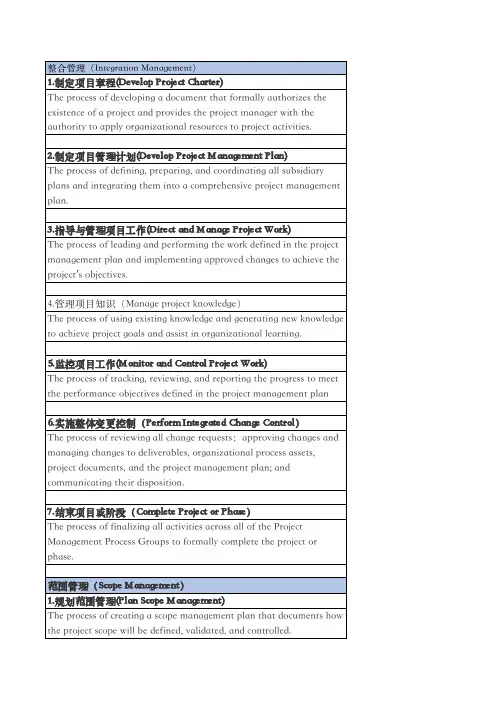
十个Knowledge Areas:1. 项目范围管理(Project Scope Management)2. 项目进度管理(Project Schedule Management)3. 项目成本管理(Project Cost Management)4. 项目质量管理(Project Quality Management)5. 项目资源管理(Project Resource Management)6. 项目沟通管理(Project Communications Management)7. 项目风险管理(Project Risk Management)8. 项目采购管理(Project Procurement Management)9. 项目干系人管理(Project Stakeholder Management)10.项目整合管理(Project Integration Management)。
Document Title: Integrated SolutionsIntroductionIn today's fast-paced and competitive business environment, companies seek innovative ways to enhance efficiency, streamline operations, and achieve sustainable growth. One approach that has gained significant attention is the integration of various systems and strategies within an organization. This document explores the concept of integrated solutions, their benefits, andthe steps involved in implementing such solutions.I. What are Integrated Solutions?Integrated solutions refer to the combination of various systems, processes, and strategies within a company to create a seamless and interconnected framework. This integration allows for data sharing, improved communication, and enhanceddecision-making across different departments and functions.II. Benefits of Integrated Solutions1. Enhanced Efficiency: Integrated solutions eliminate redundancy and streamline processes, resulting in improved productivity and reduced operational costs. Automation and synchronized data ensure that information flows seamlessly between different systems, reducing thelikelihood of human error and eliminating the need for manual data entry.2. Improved Decision-Making: Integrated solutions provide organizations with a holistic view of their operations, enabling better decision-making. Real-time data integration allows for accurate and up-to-date information, empowering managers tomake informed decisions quickly and effectively.3. Increased Customer Satisfaction: Integrated solutions enable companies to have a unified view of their customers, ensuring consistent and personalized interactions at every touchpoint. Through integrated customer relationship management (CRM) and enterprise resource planning (ERP) systems, businesses can enhancecustomer service, tailor offerings, and improve overall customer satisfaction.4. Scalability and Growth: Integrated solutions provide a solid foundation for scalable growth. By combining various systems and strategies, organizations are better equipped to adapt to changing market conditions, expand into new markets, and introduce new products or services.III. Steps to Implement Integrated SolutionsImplementing integrated solutions requires careful planning, coordination, and collaboration among different stakeholders. The following steps can guide organizations in successfully integrating their systems and strategies:1. Assess Current Systems: Evaluate existing systems, processes, and technologies to identify gaps and areasin need of improvement. Determine the specific goals and objectives that the integrated solutions should address.2. Define Requirements: Clearly define the requirements and functionalities that the integrated solutions should have. Identify the key stakeholders and involve them in the decision-making process to ensure that all relevant needs and perspectives are considered.3. Choose the Right Solution: Conduct comprehensive research to identify suitable solutions that align with the organization's requirements. Consider factors such as scalability, ease of integration, vendor support, and cost-effectiveness.4. Plan Implementation: Develop a detailed implementation plan that outlines the necessary steps, timelines, and responsibilities. Consider potentialrisks and develop contingency plans to minimize disruption during the transition.5. Integration and Testing: Begin integrating the chosen solutions into the existing systems. Ensure that data integration is seamless and that all processes and functionalities work as intended. Conduct rigorous testing to identify and resolve any issues or glitches.6. Training and Change Management: Provide adequate training to employees on using the integrated solutions effectively. Additionally, focus on change management to ensure smooth adoption and acceptance of the new systems and processes.7. Monitor and Improve: Regularly monitor the performance of the integrated solutions and gather feedback from users. Continuouslyanalyze metrics and make necessary adjustments to optimize efficiency and address any emerging challenges.ConclusionIntegrated solutions offer organizations a multitude of benefits, including enhanced efficiency, improved decision-making, increased customer satisfaction, and scalability for future growth. By carefully assessing existing systems, defining requirements, andfollowing a well-planned implementation process, organizations can successfully integrate their systems and strategies, paving the way for increased competitiveness and sustained success.。
项目总体规划及流程的英语Project Overall Planning and Process.Project planning and execution are crucial aspects of any successful endeavor. They involve meticulous consideration of all factors that could potentially affect the project's outcome, from inception to completion. This comprehensive process ensures that the project runs smoothly, stays on track, and meets its objectives within the allocated timeframe and budget.1. Project Initiation.The project begins with an idea or a need that requires a solution. This idea is then formalized into a project proposal, which outlines the objectives, scope, expected outcomes, and potential resources required. The proposal is reviewed and approved by stakeholders, who provide the necessary funding and authorization for the project to commence.2. Project Planning.Once the project is approved, the planning phase begins. This involves creating a detailed project plan thatoutlines the specific tasks, activities, and resources required to complete the project. The plan also includes a timeline, budget, and risk management strategy. Additionally, it identifies the key personnel responsiblefor executing each task and managing the project overall.3. Project Execution.During the execution phase, the project plan is implemented. This involves allocating resources, assigning tasks to team members, and monitoring progress against the established timeline and budget. Regular meetings are conducted to review progress, identify any issues or bottlenecks, and make necessary adjustments to the plan.4. Project Monitoring and Control.Monitoring and control are essential to ensure that the project remains on track. This involves tracking progress, comparing it to the plan, and taking corrective action when necessary. It also involves managing changes to the scope, timeline, or budget that may arise during the project's lifecycle.5. Project Closure.Once the project is completed, the closure phase begins. This involves formalizing the project's completion, conducting a post-project review to identify lessonslearned and areas for improvement, and documenting the project's outcomes. Additionally, the project team is disbanded, and the project is archived for future reference.Throughout the project lifecycle, effective communication and collaboration among project team members are crucial. This ensures that information flows freely, issues are identified and addressed promptly, and theproject remains on track.Moreover, project management software and tools can greatly assist in managing the project's lifecycle. These tools help in task scheduling, resource allocation,tracking progress, managing changes, and facilitating communication among team members.In conclusion, project planning and execution is a comprehensive process that requires meticulous attention to detail and effective collaboration among all stakeholders. By following a structured approach and utilizing the available tools and resources, projects can be successfully delivered within the allocated timeframe and budget, meeting or exceeding their objectives.。
Civil engineering projects are complex and multifaceted endeavors that require careful planning, coordination, and execution to ensure successful completion. Effective project management is crucial in achieving the project's objectives, maintaining quality standards, and controlling costs. This article discusses the key aspects of civil engineering project management.1. Project PlanningThe first step in civil engineering project management is to plan the project. This involves defining the project's scope, objectives, deliverables, and constraints. A detailed project plan should be developed, including the project schedule, budget, and resources required. The plan should also outline the project's milestones and key performance indicators (KPIs) to measure progress.2. Team ManagementA civil engineering project requires a diverse team of professionals, including engineers, architects, contractors, and subcontractors. Effective team management is essential to ensure that all team members are aligned with the project's objectives and working together towards a common goal. This involves assigning roles and responsibilities, facilitating communication, and resolving conflicts.3. Risk ManagementRisk management is a critical aspect of civil engineering project management. Identifying potential risks and developing strategies to mitigate them is essential to prevent project delays and cost overruns. This involves conducting risk assessments, creating risk response plans, and monitoring risks throughout the project lifecycle.4. Quality ControlMaintaining quality standards is crucial in civil engineering projects. Quality control processes should be implemented to ensure that all project deliverables meet the required specifications. This includesinspecting work progress, conducting quality audits, and implementing corrective actions when necessary.5. Cost ManagementControlling costs is another important aspect of civil engineering project management. A budget should be prepared to estimate theproject's costs, and measures should be implemented to monitor and control costs throughout the project lifecycle. This involves tracking expenses, identifying cost-saving opportunities, and managing change orders.6. Communication ManagementEffective communication is essential for the success of a civil engineering project. Communication management involves establishing clear lines of communication among all project stakeholders, including clients, contractors, and subcontractors. Regular meetings, progress reports, and status updates should be provided to ensure that everyoneis informed and aligned with the project's objectives.7. Contract ManagementContract management is a critical aspect of civil engineering project management. Contracts should be carefully reviewed and managed to ensure that all parties' rights and obligations are clearly defined. This involves managing contract changes, handling disputes, and ensuring compliance with contractual terms.8. Project ClosureProject closure is the final phase of civil engineering project management. This involves reviewing the project's performance against the established objectives, documenting lessons learned, and transitioning the project to operations or maintenance. A formal project handover should be conducted to ensure that the client is satisfied with the project's outcome.In conclusion, effective civil engineering project management is essential for achieving project objectives, maintaining qualitystandards, and controlling costs. By focusing on planning, team management, risk management, quality control, cost management, communication management, contract management, and project closure, project managers can ensure the successful completion of civil engineering projects.。
IntroductionConstruction project management is an intricate process that involves the planning, coordination, and supervision of a construction project from inception to completion. Ensuring high-quality and high-standard outcomes in this context is paramount for meeting client expectations, ensuring structural integrity, and fostering sustainable development. This essay delves into the multifaceted nature of achieving these objectives by examining key aspects such as quality control, risk management, stakeholder engagement, technology utilization, sustainability, and regulatory compliance.1. Quality ControlThe foundation of high-quality and high-standard construction lies in robust quality control systems. This encompasses a comprehensive approach that starts with defining clear quality standards and specifications, followed by systematic monitoring, inspection, and testing throughout the project lifecycle. Quality control measures should be aligned with industry standards such as ISO 9001 or specific national or regional codes, and tailored to the unique requirements of each project.Effective quality control necessitates the implementation of stringent material procurement procedures to ensure that only approved, high-grade materials are used. Regular on-site inspections by qualified professionals, coupled with non-destructive testing methods, help detect and rectify any deviations from the predefined standards promptly. Moreover, the use of advanced software tools for quality management, like Building Information Modeling (BIM), can enhance precision, minimize errors, and facilitate real-time monitoring and reporting.2. Risk ManagementHigh-quality and high-standard construction projects are inherently risk-averse. A proactive and systematic approach to risk management is vital to identify potential threats, assess their likelihood and impact, and develop strategies to mitigate or eliminate them. Risks can stem from various sources, including design flaws, supply chain disruptions, environmental factors, labor disputes, and regulatory changes.A well-implemented risk management framework includes risk identification workshops, quantitative and qualitative risk analysis, and the formulation of risk response plans. Regular risk reassessments and effective communication channels help maintain situational awareness and ensure swift responses to emerging risks. Additionally, contingency planning and the establishment of reserve funds provide a financial buffer against unforeseen events that may compromise project quality or standards.3. Stakeholder EngagementSuccessful high-quality and high-standard construction projects heavily rely on effective stakeholder engagement. This involves establishing open and transparent communication channels with clients, designers, contractors, suppliers, regulatory authorities, and local communities. Regular meetings,site visits, and progress reports keep stakeholders informed about project developments, while their feedback and concerns are actively solicited and addressed.Moreover, stakeholder engagement fosters collaboration and alignment around project goals, quality benchmarks, and performance targets. It enables early identification and resolution of issues, promotes innovation and knowledge sharing, and enhances overall stakeholder satisfaction. Engaging stakeholders in decision-making processes, particularly concerning critical quality-related matters, further reinforces their commitment to upholding high standards.4. Technology UtilizationTechnology plays a transformative role in enhancing the quality and standard of construction projects. Advanced technologies such as BIM, drones, 3D printing, artificial intelligence, and Internet of Things (IoT) devices offer unprecedented levels of precision, efficiency, and data-driven decision-making. BIM, for instance, facilitates seamless collaboration among project stakeholders, reduces design conflicts, and enables virtual simulations for clash detection and performance analysis.Drones equipped with high-resolution cameras and sensors can conduct aerial surveys, monitor construction progress, and detect potential quality issues. IoT devices and sensors can provide real-time data on structural health, energy consumption, and environmental conditions, enabling proactive maintenance and continuous improvement. Artificial intelligence algorithms can analyze this data to predict failures, optimize resource allocation, and automate quality control processes.5. SustainabilityIn today's environmentally conscious era, high-quality and high-standard construction projects must also demonstrate a strong commitment to sustainability. This encompasses not only minimizing the project's environmental footprint but also ensuring long-term energy efficiency, resource conservation, and social responsibility.Sustainable construction practices include using eco-friendly materials, incorporating renewable energy systems, implementing water-efficient designs, and promoting waste reduction through recycling and reuse. Green building certifications like LEED, BREEAM, or WELL provide a standardized framework for assessing and improving a project's sustainability performance. Furthermore, engaging in community outreach programs, respecting local cultures, and providing safe working conditions contribute to the project's social sustainability.6. Regulatory ComplianceFinally, adherence to relevant laws, regulations, and guidelines is essential for maintaining high-quality and high-standard construction projects. Compliance encompasses obtaining necessary permits and approvals, conforming to building codes, safety regulations, environmental laws, and labor standards. Non-compliance can result in legal penalties, project delays, reputationaldamage, and potential hazards to public safety and the environment.Regular audits, inspections, and training programs help ensure that all project participants are aware of and comply with the applicable regulations. Moreover, maintaining open communication with regulatory agencies and seeking guidance when faced with regulatory uncertainties can prevent misunderstandings and costly mistakes.ConclusionAchieving high-quality and high-standard outcomes in construction project management is a multidimensional endeavor that necessitates a holistic approach encompassing quality control, risk management, stakeholder engagement, technology utilization, sustainability, and regulatory compliance. By diligently addressing these aspects, project managers can ensure the delivery of structurally sound, functionally efficient, environmentally responsible, and socially beneficial buildings that meet or exceed client expectations and contribute to the built environment's lasting value and resilience.。
发展规划与行动计划英语Development Planning and Action Plan.In today's rapidly changing world, it's crucial for organizations and individuals alike to have a clear development planning and action plan. These plans serve as roadmaps, guiding us through the complexities of achieving our desired goals and objectives. Development planning involves the identification of areas that require improvement, setting specific targets, and outlining the strategies to achieve those targets. The action plan, on the other hand, details the specific steps that need to be taken to implement the development plan.For organizations, development planning often begins with a thorough analysis of their current state. This involves assessing various aspects such as financial performance, market position, technological capabilities, and human resources. By understanding their strengths, weaknesses, opportunities, and threats (SWOT analysis),organizations can identify the areas where they need to focus their development efforts.Once the areas of improvement are identified, specific development goals and targets should be set. These goals should be measurable, achievable, relevant, and time-bound (SMART). For example, an organization may set a goal to increase its market share by 10% within the next year. This goal is specific, measurable, and has a clear time frame.The next step is to develop an action plan thatoutlines the steps needed to achieve these goals. The action plan should include a detailed timeline, assignment of responsibilities, and identification of resources required. It should also take into account any potential risks and challenges and provide strategies to mitigate them.For example, to increase market share, an organization may decide to launch a new product or service. The action plan would then detail the steps required to develop the product, conduct market research, create a marketing plan,and launch the product successfully. It would also identify the team members responsible for each step and theresources needed to complete them.In addition to the action plan, it's important to havea monitoring and evaluation mechanism to track progress and ensure that the plan is being implemented effectively. This involves regular reviews of progress, comparison with targets, and identification of any deviations. If necessary, adjustments can be made to the plan to ensure that thegoals are still achievable.For individuals, the development planning and action plan process is similar but with a different focus. Instead of focusing on organizational goals, individuals focus on personal and professional development. They identify areas where they want to improve, set personal goals, and create an action plan to achieve those goals.For example, an individual may want to improve their skills in a particular area or achieve a certainprofessional certification. Their action plan would detailthe steps they need to take to achieve this, such as attending courses, practicing regularly, or seeking mentorship.In conclusion, development planning and action plans are crucial for both organizations and individuals. They provide a clear roadmap to achieving desired goals and objectives, ensuring that efforts are focused and resources are used effectively. By regularly monitoring and evaluating progress, adjustments can be made to ensure that the plan remains on track and the goals are achieved.。
Integrated Planning and Control for Convex-bodied Nonholonomic systems using Local Feedback Control Policies David C.Conner,Alfred A.Rizzi,and Howie ChosetCMU-RI-TR-06-34August2006Robotics InstituteCarnegie Mellon UniversityPittsburgh,Pennsylvania15213c2006Carnegie Mellon UniversityAbstractWe present a method for defining a hybrid control system capable of simultaneously addressing the global navigation and control problem for a convex-bodied wheeled mobile robot navigating amongst obsta-cles.The method uses parameterized continuous local feedback control policies that ensure safe operationover local regions of the free configuration space;each local policy is designed to respect nonholonomicconstraints,bounds on velocities(inputs),and obstacles in the environment.The hybrid control systemmakes use of a collection of these local control policies in concert with discrete planning tools in order toplan,and replan in the face of changing conditions,while preserving the safety and convergence guaran-tees of the underlying control policies.In this paper,we provide details of the system models and policydefinitions used to validate the approach in simulation and experiment with a convex-bodied wheeled mo-bile robot.This work is one of thefirst that combines formal planning with continuous feedback controlguarantees for systems subject to nonholonomic constraints,input bounds,and non-trivial body shape.c2006Carnegie Mellon iContents1Introduction1 2Related Work32.1Motion Planning and Control with Nonholonomic Constraints (3)2.2Sequential Composition (4)3General Framework73.1System Models (7)3.2Generic Policy Requirements (8)3.2.1Simple Inclusion Tests (8)3.2.2Contained in Free Space (9)3.2.3Conditionally Positive Invariant (10)3.2.4Finite Time Convergence (10)3.3Discrete Planning in Space of Policies (11)3.3.1Extensions to Prepares Definition (11)3.3.2Planning in Policy Space (12)4Local Policy Definitions154.1Inclusion Test (18)4.2Free Configuration Space Test (18)4.3Conditional Invariance Test (19)4.4Vector Field Definition and Convergence Test (20)5Policy Deployment Technique23 6Current Results276.1Robot System and Implementation (27)6.2Navigation Experiments (29)6.3Task Level Planning Simulations (30)7Conclusion33 A Free Space Testing37 References41c2006Carnegie Mellon iii1IntroductionThe problem of simultaneously planning and controlling the motion of a convex-bodied wheeled mobile robot in a cluttered planar environment is challenging because of the relationships among control,nonholo-nomic constraints,and obstacle avoidance.The objective is to move the robot through its environment such that it arrives at a designated goal set without coming into contact with any obstacle,while respecting the nonholonomic constraints and velocity(input)bounds inherent in the system.Conventional approaches addressing this problem typically decouple navigation and control[12,31,33]. First,a plannerfinds a path,and then a feedback control strategy attempts to follow that path.Often the methods assume a point or circular robot body;other non-trivial robot body shapes complicate the problem offinding a safe path,as the path must be planned in the free configuration space of the robot.This leaves the challenging problem of designing a control law that converges to the one-dimensional path,while remaining safe with respect to obstacles.We address the coupled navigation and control problem by generating a vectorfield along which the robot can“flow.”Unfortunately,determining a global vectorfield that satisfies all of these objectives for constrained systems can be quite difficult.Our approach,inspired by the idea of sequential composition[11], uses a collection of local feedback control policies coupled with a switching strategy to generate the vector fiposing these relatively simple policies induces a piecewise continuous vectorfield over the union of the policy domains.A policy is specified by a configuration dependent vectorfield defined over a local region of the robot’s free configuration space,termed a cell.From this vectorfield and knowledge of the current robot state,the control inputs are determined such that the closed-loop dynamicsflows to the specified policy goal set within the cell.Figure1shows four paths induced by invoking the local policies for four different initial conditions in the robot experiments,as will be discussed in Section6.Figure1:Experimental results of four robot runs using the proposed hybrid control framework.An explicit desired path is never calculated,the path is induced by sequentially chaining local feedback control policies together;the policy ordering is determined by a discrete planner.The induced path preserves the local guarantees of the local polices,and is thus free of collision while respecting the system constraints.c2006Carnegie Mellon1A discrete transition relation represented by a graph is induced by the transition between the domain of one policy to the domain of a second policy containing the policy goal set of thefirst.On-line planning,and re-planning under changing conditions,becomes more tractable on the graph,allowing us to bring numerous discrete planning tools to bear on this essentially continuous problem.By sequencing the local policies according to the ordering determined by a discrete planner,the closed loop dynamics induce the discrete transitions desired by the discrete plan.The overall hybrid(switched)control policy responds to system perturbations without the need for re-planning.In the face of changing environmental conditions,the discrete graph allows for fast online re-planning,while continuing to respect the system constraints.By coupling planning and control in this way,the hybrid control system plans in the discrete space of control policies;thus,the approach represents a departure from conventional techniques.A“thin”path or trajectory is never explicitly planned;instead,the trajectory induced by the closed-loop dynamicsflows along the vectorfield defined by the active policy,which is chosen according to an ordering determined by a discrete planner.A plan over the discrete graph associated with the collection of policies corresponds to a“thick”set of configurations within the domains of the associated local policies.This approach offers guaranteed convergence over the union of the local policy domains.For the method to be complete,the entire free configuration space must be covered by policy domains(cells).This is a difficult problem due to the multiple constraints on the robot dynamics.Herein,the focus is on deploying a “rich enough”collection of policies that enables the navigation problem to be addressed over the bulk of the free configuration space.This paper describes the basic requirements that any local policy must satisfy to be deployed in this framework;each local policy must be provably safe with respect to obstacles and guarantee convergence to a specified policy goal set,while obeying the system constraints within its local domain.We develop a set of generic policies that meet these requirements,and instantiate these generic policies in the robot’s free configuration space.The underlying equations are detailed,and examples are provided.Finally,a concrete demonstration of controlling a real mobile robot using a collection of local policies is described.2c2006Carnegie Mellon2Related WorkThe approach advocated in this paper maintains the coupling between planning and control,unlike con-ventional approaches that decouple the problem into a path planning problem and a path-following control problem.This section presents a brief overview of conventional approaches,and concludes with a discussion of the sequential composition approach that motivates this work.2.1Motion Planning and Control with Nonholonomic ConstraintsThe control of systems with nonholonomic differential constraints is more complex than control of purely holonomic1systems.This section contains an overview of techniques used to plan paths and trajectories for nonholonomic systems,and address four basic control problems for nonholonomic systems–stabilization, path-following,trajectory-tracking,and point-to-point steering[18,30,43].The discussions give insight into the difficulties associated with nonholonomic motion planning and control.For a more thorough discussion and reference list,refer to[30,32,33].To recognize the complexity introduced by nonholonomic constraints,consider the“simple”problem of stabilizing a system about a given equilibrium point.Brockett’s theorem provides necessary conditions for the existence of a smooth,time-invariant feedback control law that stabilizes the system about the given point[10].It is well known that many nonholonomic systems,although small-time locally controllable,fail Brockett’s test[30,43].This precludes the use of conventional feedback control based on potential functions. Several classes of stabilizing feedback control policies have been developed:discontinuous time invariant, time varying,and hybrid control policies[30].Given the complexity of this control task,it is no surprise that the coupled navigation and control task is more complex than for holonomic systems.Many approaches addressing the coupled navigation and control problem for nonholonomic systems de-compose the problem into a motion planning problem,followed by a control problem.A common planning approach is to pretend the system is holonomic and hope for the best.In the holonomic case,the path or tra-jectory can be planned using any of a number of methods[12,35].Grid-based search algorithms are popular in path planning,as are roadmap methods such as V oronoi diagrams.Potential function methods,while not necessarily complete,are also widely used in path/trajectory planning.Given a path through the environment,a path-following algorithm is then used to converge to the desired path.There are two basic formulations to path-following.In thefirst,a designated point on the robot traces a given path in the workspace,without concern for orientation[15].This may fail in cluttered environments as the designated point may exactly follow a safe path,yet still allow the system to collide with an obstacle at another point on the robot body.The second formulation attempts to track position and orientation of a path in the free configuration space[17].If the environment is not overly cluttered,so that deviations are not catastrophic,path following may work well.In fact,if a system is small-time locally controllable,any continuous path can be approximated arbitrarily well[34].Unfortunately,the methods used to control the system along arbitrary paths often lead to highly oscillatory motions that require great control effort.If the path does not respect the system constraints, the resulting motions may require an inordinate number of reversals to follow the desired path.One approach to address this problem is to plan a path without regard to nonholonomic constraints,and perturb the path to respect nonholonomic constraints[51].Techniques that consider the nonholonomic constraints during planning typically use only a discrete set of feasible motions.The shortest feasible path(SFP)metric is used to plan paths that approximate a holonomic path using afinite number of motions[42].The motions are selected by choosing the shortest feasible path to a point on the holonomic path intersecting the largest ball defined by the SFP metric[56].Dynamic programming methods determine an optimal path for a discrete set of controls(e.g.hard left,soft left,straight,soft right,hard right)[3,21,36].Probabilistic roadmaps(PRM)and rapidly-exploring random trees(RRT)are other discrete approaches to determining feasible paths for nonholonomically constrained systems[37,54].With the exception of dynamic programming,these discrete methods are not feedback based,and require replanning if the system deviates from the desired path.Even if the planned path respects the nonholonomic constraints,the path must be followed by the robot. The presence of nonholonomic constraints renders path-following a non-linear controls problem.Control laws based on a Lyapunov analysis[17]or feedback linearization[18,50]are common.Most path-following algorithms assume continuous motion,with a non-stationary path defined for all time.This(temporarily) avoids Brockett’s problem with stabilization to a point[15,17].The path-following control policy asymptot-ically brings the error between the desired path and the actual path to zero.Typically,the control policy is constructed for a specific vehicle and class of paths[2,17,15,55].The path-following control laws are unaware of environmental obstacles;therefore,for a nonzero initial error or perturbation during motion,the system may collide with an obstacle.Path-following may be coupled with local obstacle avoidance,but this may invalidate the convergence guarantees.Thus,if the errors are large enough,the paths must be replanned,starting from the current location.In addition to path-planning,trajectories that specify when the system arrives at points along the path may be planned[17,50].Trajectory-tracking problems can be problematic if the system is subject to a constraint that delays the tracking[17].In this case,the accumulated error may make the system unstable or require unreasonably high inputs.Another possible problem is that trajectory-tracking controls may switch directions for certain initial conditions[50].Unless the time matching along the trajectory is crucial,path-following is often a better formulation[17,50].In related work,several methods–including sinusoidal inputs,piecewise constant inputs,optimal control, and differentiallyflat inputs–solve the point-to-point steering problem between two positions using open loop controls[34,43].These methods are sometimes incorporated into the discrete planning systems.Each of these methods is an open loop control method that does not respect obstacles.Collision detection must be performed after the path is found to determine feasibility in a cluttered environment[27].These point-to-point steering methods are strictly open loop,and not suitable for feedback control.The inevitable errors necessitate repeated applications to induce convergence to the goal point.There have been a few attempts to address the coupled navigation and control problem for nonholonomic systems.A method based on potentialfields uses resistive networks to approximate the nonholonomic con-straints[14].This approach requires a discretization of the configuration space,and is therefore subject to numerical difficulties when calculating derivatives necessary for feedback control.Other approaches define integral sub-manifolds in configuration space that contain the goal[25,29,41].On the sub-manifold,the nonholonomic constraints are integrable,and the control naturally respects the constraints.The approaches drive the system to the sub-manifold,and then along the sub-manifold to the goal.While these methods are suitable for feedback control implementations,determination of a suitable manifold is sometimes difficult. For systems where the stable manifold is not given in closed form,an iterative process is used to approximate the manifold.The approaches also involve designing several functions that require insight into the specific problem and system constraints.2.2Sequential CompositionThe research presented in this paper uses the technique of sequential composition,which enables the con-struction of switched control policies with guaranteed behavior and provable convergence properties[11].The original form of sequential composition uses state regulating feedback control policies,whose do-mains of attraction partition the state space into cells[11].The control policy can be thought of as a funnel, as shown in Figure2,where the vertical represents the value of a Lyapunov function,and the domain is the 4c2006Carnegie MellonFigure2:An idealized Lyapunov function and its associated domain of attraction rep-resented by its shadow on the state space. The goal point is shown as a large dot within thedomain.Figure3:Composition of control policies leads to an enlarged domain of attraction.Note that the active policy switches to the highest priority policy as soon as the state enters its domain.“shadow”cast by the funnel on the state space below[11].The domain is the safe domain of attraction, which is the largest positive invariant region that does not intersect an obstacleThe basic idea behind sequential composition is to compose multiple control policies in a way that enlarges the overall domain of attraction,while preserving the underlying convergence guarantees.The approach specifies the goal of one policy to lie within the domain of another policy.By properly prioritizing the policies,and switching to a higher priority policy once the state enters the domain of the higher priority policy,it is possible to construct a switching control policy with a larger domain of attraction than any single policy[11].The domain of attraction of the switched policy is equal to the union of the domains of the component policies,as shown in Figure3.By composing policies with limited domains,constraints in the state space can be respected while building an almost globally convergent control policy.In this way,the free state space may be covered by incrementally covering an additional region of the free state space.The policy composition is based on a formal notion of prepares[11].For a given control policy,, denote the domain of the policy and the goal.Given two control policies,is said to prepare,denoted,if.Let afinite collection of instantiated control policies, ,defined over the free state space of a given system be given,and assume at least one policy stabilizes the overall goal.The prepares relationship between any two policies in the collection induces a directed graph,,over the collection of instantiated control policies.In general the policy graph is cyclic;however,an acyclic graph,,may be generated over the collection of policies by searching the original graph breadthfirst,beginning at the node corresponding to the policy that stabilizes the overall goal, and adding only those links and nodes that connect back to previously visited nodes.The acyclic graph is a partial order over the collection of control policies.By construction,the partial order graph is a connected graph containing a node corresponding to the policy that stabilizes the goal.Given the collection of policies ,the switching strategy defined by the associated partial order induces an overall switching control policy, denoted.The union of the domains of the instantiated policies included in the partial order gives the domain of the overall policy;that is(1) c2006Carnegie Mellon5The overall control policy induced by sequential composition is fundamentally a hybrid control policy[6, 8,24].The composition of these local policies in a hybrid systems framework enables analysis on the discrete representation of the transitions between policy domains[8,11].We may analyze whether a goal node is reachable using the partial order graph,which functions as afinite state automata[24].Reachability of the goal state and decidability of the navigation problem for a particular collection of policies can be determined by the discrete transitions on,without analyzing the underlying continuous system[24].This analysis may be done prior to,or during,construction of the partial order.The stability of the underlying control policies guarantees the stability of the overall switched policy because the partial order results in monotonic switching[11].This obviates the need for complex hybrid sta-bility analysis of the form given in[5,7,16,38].Disturbances are robustly handled provided their magnitude and rate of occurrence is small compared to the convergence of the individual policies[11].The system in[11]uses multiple policies to demonstrate the inherent robustness of the technique.The deployment of the generic policies–including specification of the setpoints,control policy gains,and pol-icy ordering–is accomplished manually.The deployment uses conservative approximations of the policy domains obtained through experimentation and simulation.Sequential composition-like techniques have been applied to mobile robots.Many examples are for systems without nonholonomic constraints,where the policies are defined over simple cells–polytopes and balls–in configuration space[47,48,57].Other approaches have used optimal control techniques on discrete state space representations to encode local policies[9,22].Sequential composition has also been used to control wheeled mobile robots using visual servoing[28, 44].In these cases,the local control policies were designed based on careful analysis of the system,its constraints,and the problem at hand.These later approaches have the key feature that many of the individual policies are not designed to converge to a single point.In the later example,the“goal”of the highest priority policy is to drive through a doorway[44].It is assumed that another control policy becomes active after the vehicle passes through the doorway.This idea offlow-through policies inspired work where generic policies are defined over polytopes that partition the environment into local cells[13].This work was followed by similar approaches that used different methods of defining the control vectorfields over the polytopes[4,40].These methods were originally developed for idealized holonomic systems,but may be applied to point nonholonomic systems using feedback linearization[4].However,these approaches do not apply to systems with non-trivial body shapes,and cannot guarantee that the linearized system does not“cut a corner”between polytopes and collide with an obstacle.A key feature of these approaches is that the policies are generic,and are therefore amenable to automated deployment[4,13,40].These approaches also formed the base for later work in applying discrete planning techniques to specify logical constraints on the ordering of the local policies[19,20].Using the policy graph, ,a model checking system generates an open loop sequence of policies whose closed-loop behaviors satisfy the tasks specified in temporal logic.In addition to model checking,there has been substantial work in the problem of planning and replanning on discrete graphs.The D*algorithm,originally developed for grid based path planning,facilitates fast replanning based on changes in the graph cost structure[53].A similar,but algorithmically different version, called D*-lite has been applied to graph structures;including those,such as Markov Decision Processes (MDP),that support non-deterministic outcomes[39].6c2006Carnegie Mellon3General FrameworkThis section presents the framework used to address the navigation problem described in this paper.First,a brief overview of the robot modeling framework is given.Next,the generic requirements for the the local policies are presented.This section concludes with an overview of planning based on the discrete transition graph induced by the policies.3.1System ModelsThe robot system consists of a single body that navigates through a planar environment that is cluttered with obstacles.The planar environment,or workspace,is a bounded subset.Letdenote the position and orientation,relative to the world frame,of a reference frame attached to the robot body.As the robot moves through its workspace,evolves on the manifold.To address the navigation problem,the robot body must move along a path that reaches the overall goal, while avoiding obstacles along the way.Let denote the two-dimensional set of workspace points occupied by the body at position and orientation.The obstacles in the workspace are represented as the union over afinite set of convex regions.Thus,for all body positions and orientations,,along a collision free path,The robotic systems considered in this paper are driven by wheels in contact with the planar environment; the wheel-to-ground contact generates nonholonomic velocity constraints.The rotation of these wheels may be represented by internal shape variables[1].Thus,the robot configuration is fully specified as ,where denotes the shape variables.The shape variable velocities are controlled via control inputs.For kinematic systems,;for second-order dynamical systems.This paper is restricted to simple robot models where the nonholonomic constraints determine a linear mapping,, between velocities in the shape space and the velocity,,of the bodyfixed frame.The robot is induced to move along a path by application of the control inputs;the closed-loop dynamics determine the velocity via the mapping.The velocity determines the robot path.The control problem is to specify control inputs such that the system moves along a collision free path and reaches the overall goal.To be a valid control,the inputs must be chosen from the bounded input space.As bounded inputs and the mapping constrain,the navigation problem is tightly coupled to the control problem.To address the navigation and control problem in a coupled manner,we define local control policies over local regions of that are termed cells.Let denote the feedback control policy in a collection of policies and let denote the local cell.Define the cell in a subset of that locally represents the configuration space;the cells are restricted to compact,full dimensional subsets of without punctures or voids.It is assumed that the boundary of the cell,,has a well defined unit normal,, that exists almost everywhere.The policy goal set,denoted,is a designated region in the local cell; that is.In this framework,the coupled navigation and control problem of moving the robot body through the space of free positions and orientations of the bodyfixed frame is converted to a problem of specifying safe feedback control policies over the local cells,and then composing these local policies to address the larger navigation problem.Over each local cell,define a feedback control policy,where denotes the tangent bundle over the robot’s configuration space.In other words,the local policy maps the current robot state,whose configuration falls within the local cell,to an input in the bounded set of inputs associated with the policy.The policy must be designed such theflow of induced by entersc2006Carnegie Mellon7Figure4:A cell defines a local region in the space of robot body positions and orientations.In this example, the cell is funnel shaped and the designated goal set is the small opening at the point of the funnel..Thus,instead of a specific path,the closed-loop dynamics of the local policy induce a vectorfield flow over the cell that enters.3.2Generic Policy RequirementsFor a local policy to be useful in the sequential composition framework,it must have several properties.First, to be practical,the local policies must have efficient tests to see if a specific local policy can be safely used; that is the system must be able to determine if the current robot state is within the domain of a given policy. Second,to induce safe motion,the cell must be contained in the space of free body positions and orientations so that collision with any obstacle is not possible while the body frame is within this cell.Third,under the influence of the policy,the induced trajectories must reach the policy goal set defined within the local cell without departing the associated cell from any initial position and orientation within the cell.Finally,the system must reach the designated goal set infinite time for any initial condition within the cell.The requirements discussed below are generic with respect to the given robot model and any specific cell definition.The focus in the remainder of this section is on the generic policy requirements that enable the proposed hybrid control framework to work with a variety of system models.3.2.1Simple Inclusion TestsA given policy is safe to activate if the robot state is within the policy domain,.The domain,which depends upon the policy definition,generally specifies both configurations and velocities.As the policies are defined over,thefirst test of domain inclusion is that.For kinematic systems, because the state is simply the configuration.Therefore,only the cell inclusion test is needed to check to see if a policy is safe to activate for the simple models considered in this paper.8c2006Carnegie Mellon。