Weak effects in proton beam asymmetries at polarised RHIC and beyond

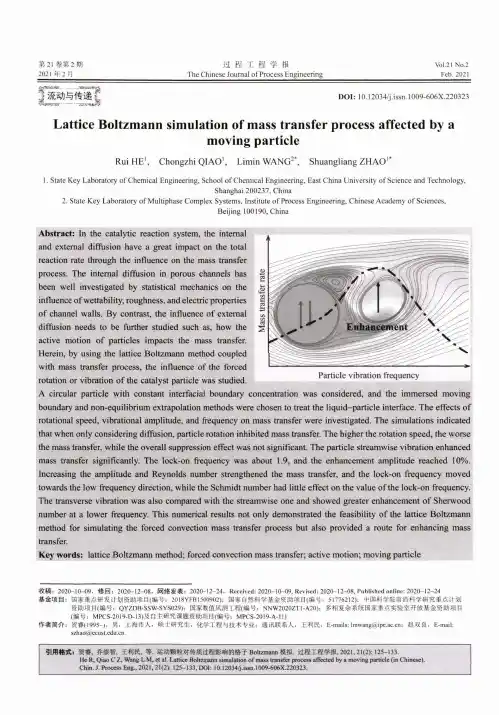
第21卷第2期2021年2月过程工程学报T h e Chinese Journal of Process EngineeringVol.21 No.2 Feb. 2021Particle vibration frequencyDO I : 10.12034/j.issn. 1009-606X.220323Lattice Boltzmann simulation of mass transfer process affected by a moving particleRui HE 1, Chongzhi QIAO 1, Limin WANG 2*, Shuangliang ZH AO 1*1. State K e y Laboratory of Chemical Engineering, School of Chemical Engineering, East China University of Science and Technology,Shanghai 200237, China2. State K e y Laboratory of Multiphase Compl e x Systems, Institute of Process Engineering, Chinese A c a d e m y of Sciences,Beijing 100190, ChinaAbstract : In the catalytic reaction system , the internaland external diflfusion have a great impact on the total reaction rate through the influence on the mass transfer process . The internal diffusion in porous channels has been well investigated by statistical mechanics on the influence o f w ettability , roughness , and electric properties of channel walls . By contrast , the influence of external diffusion needs to be further studied such as , how the active motion o f particles impacts the mass transfer .Herein , by using the lattice Boltzmann method coupled with mass transfer process , the influence of the forced rotation or vibration o f the catalyst particle was studied .A circular particle with constant interfacial boundary concentration was considered , and the immersed moving boundary and non-equilibrium extrapolation methods were chosen to treat the liquid-particle interface . The effects o f rotational speed , vibrational amplitude , and frequency on mass transfer were investigated . The simulations indicated that when only considering diffusion , particle rotation inhibited mass transfer . The higher the rotation speed , the worse the mass transfer , while the overall suppression effect was not significant . The particle streamwise vibration enhanced mass transfer significantly . The lock-on frequency was about 1.9, and the enhancement amplitude reached 10%. Increasing the amplitude and Reynolds number strengthened the mass transfer , and the lock-on frequency moved towards the low frequency direction , while the Schmidt number had little effect on the value of the lock-on frequency . The transverse vibration was also compared with the streamwise one and showed greater enhancement o f Sherwood number at a lower frequency . This numerical results not only demonstrated the feasibility of the lattice Boltzmann method for simulating the forced convection mass transfer process but also provided a route for enhancing mass transfer .Key words : lattice Boltzmann method ; forced convection mass transfer ; active motion ; moving particle收稿：2020-10-09，修回：2020-12-08，网络发表：2020-12-24，Rece 丨ved: 2020-10-09, Revised: 2020-12-08, Pub 丨ished online: 2020-12-24基金项目：国家重点研发计划资助项目(编号：2018Y FB1500902);国家自然科学基金资助项目(编号：51776212):中国科学院前沿科学研宂重点计划资助项目(编号：QYZDB-SSW -SYS029);国家数值风洞工程(编号：NNW2020ZT1-A20);多相复杂系统国家重点实验室幵放基金资助项目 (编号：MPCS-2019-D-13)及自主研宄课题资助项目(编号：MPCS-2019-A-11)作者简介：贺窨(1995-),男，上海市人，硕士研宄生，化学工程与技术专业•，通讯联系人，王利民，E-mails: *************.cn:赵双良，E-mail:***************.cn.引用格式：贺眘，乔崇智，王利民，等.运动颗粒对传质过程影响的格子Boltzmann 模拟.过程工程学报，2021，21(2):丨25-133.He R, Qiao C Z, Wang L M, et al. Lattice Boltzmann simulation o f mass transfer process affected by a moving particle (in Chinese). Chin. J. Process Eng., 2021, 21(2): 125-133, DOI: 10.12034/j.issn. 1009-606X.220323.Bs J 3J C /5U21S S C 3S126过程工程学报第21卷运动颗粒对传质过程影响的格子Boltzmann模拟贺睿、乔崇智、王利民2，赵双良1I.华东理工大学化工学院，化学工程联合国家重点实验室，上海2002372.中国科学院过程工程研究所多相复杂系统国家重点实验室，北京100190摘要：颗粒的主动运动对传质过程有重要影响。

Shock Waves(2008)17:409–419DOI10.1007/s00193-008-0124-3ORIGINAL ARTICLENumerical investigation of ethyleneflame bubble instability induced by shock wavesGang Dong·Baochun Fan·Jingfang YeReceived:3August2006/Revised:28November2007/Accepted:26February2008/Published online:19March2008©Springer-Verlag2008Abstract In this paper,the ethylene/oxygen/nitrogen premixedflame instabilities induced by incident and reflec-ted shock wave were investigated numerically.The effects of grid resolutions and chemical mechanisms on theflame bubble deformation process are evaluated.In the computatio-nal frame,the2D multi-component Navier–Stokes equations with second-orderflux-difference splitting scheme were used;the stiff chemical source term was integrated using an implicit ordinary differential equations(ODEs)solver.The two ethylene/oxygen/nitrogen chemical mechanisms,namely 3-step reduced mechanism and35-step elementary skeletal mechanism,were used to examine the reliability of chemis-try.On the other hand,the different grid sizes, x× y= 0.25×0.5mm and x× y=0.15×0.2mm,were imple-mented to examine the accuracy of the grid resolution.The computational results were qualitatively validated with expe-rimental results of Thomas et al.(Combust Theory Model 5:573–594,2001).Two chemical mechanisms and two grid resolutions used in present study can qualitatively reproduce the ethylene sphericalflame instability process generated by an incident shock wave of Mach number1.7.For the case of interaction between theflame and reflected shock waves, the35-steps mechanism qualitatively predicts the physical process and is somewhat independent on the grid resolutions, while the3-steps mechanism fails to reproduce the instability Communicated by J.F.L.Haas.G.Dong(B)·B.Fan·J.YeState Key Laboratory of Transient Physics,Nanjing University of Science and Technology,Nanjing,Jiangsu210094,People’s Republic of Chinae-mail:dgvehicle@G.DongState Key Laboratory of Explosion Science and Technology,Beijing Institute of Technology,Beijing100081,China of ethyleneflame for the two selected grid resolutions.It is concluded that the detailed chemical mechanism,which includes the chain elementary reactions of fuel combustion, describes theflame instability induced by shock wave,in spite of the fact that theflame thickness(reaction zone)is represented by1–2grids only.Keywords Ethyleneflame·Shock waves·Chemical mechanism·Grid resolutionPACS82.40.Fp·47.40.Nm·47.70.Pq1IntroductionThe interactions between shock wave and curving contact discontinuity(e.g.,cylindrical or spherical gas with different density)can lead to the Richtmyer–Meshkov instability and further enhance the mixing process of gases with the different densities.The phenomenon occurs frequently in many prac-tice processes such as Scramjet[1,2].For example,theflame instability induced by shock wave can lead to the enhance-ment of the fuel/oxidizer mixing and the increase offlame burning rate.Many studies have been focused on the issues. For the inert shock–bubble interaction case,many experi-mental(e.g.,[3,4])and numerical(e.g.,[5–8])studies have been presented within a wide range of shock wave Mach number.In these studies,the fundamental mechanisms asso-ciated with the interface instability,the vortices structure and the mixing were widely investigated.The shock–bubble interaction has been proposed as a benchmark problem for testing the numerical scheme and grid resolution in CFD [9].On the other hand,for the reactive shock–flame inter-action case,Markstein’s classical experiments[10]showed the interactions offlames with a weak shock wave and its410G.Dong et al. reflected wave for butane/air mixture.Theflame instabi-lities were clearly observed.Recently,Thomas et al.[11]performed a series of experiments which showed the signi-ficantflame acceleration induced by stronger shock wavein C2H4/O2/N2mixture.They also showed that detonationcan emerge near the reaction zone for higher incident shockwave intensity.Numerical investigations on the interactionof shock wave withflame bubble have also been reportedwidely.Picone et al.[12],firstly,reported the interaction ofhot bubble with shock wave.However,the contact disconti-nuity in their model is inert.Ton et al.[13]studied the effectof chemical reaction during the interaction between the shockwave andflame.Khokhlov et al.[14]numerically studied asingle interaction of an incident shock wave with a sinusoi-dally perturbedflame.They developed a2D reactive Navier–Stokes equations solver based on the second-order Godunovtype scheme and the adaptive mesh refinement(AMR)tech-nique.Their results revealed that theflame instability and theenhancement of burned/unburned material mixing are due tothe Richtmyer–Meshkov(RM)instability.In their followingpapers[15–17],reflected shock wave effects were furtherconsidered using the same solver.The multiple shock–flameinteractions,through RM instability,result in the highly dis-tortedflame and further lead to the deflagration-to-detonation(DDT)at the specified conditions.Khokhlov et al.’s numeri-cal investigations represent a state of the art computation ontheflame instability perturbed by shock wave.However,as aone-step lumped reaction mechanism based on the Arrheniusform was used in their model,the effect of elementary reac-tion mechanisms for hydrocarbon fuel on the shock–flameinteraction has not been taken into account.In the present paper,a shock–flame interaction processis presented numerically considering the elementary chemi-cal reactions for ethylene fuel.The effects of the differentchemical reaction mechanisms and the grid resolutions onthe shock–flame interaction are evaluated in the numericalsimulations.The experiment of the ethyleneflame bubbleinstability perturbed by shock wave by Thomas et al.[11]has been used to validate and examine the numerical results.2Numerical methods2.1Governing equationsIn the numerical model,it is assumed that the thermally per-fect ideal gas law is used,thus,the2D axisymmetric reactiveNavier–Stokes equations for multi-component system are asfollows∂U ∂t +∂(F−F D)∂x+∂(G−G D)∂y+W=S(1)where,U denotes the solutions of the Eq.(1);F and G denote the convectionfluxes in x and y directions,respectively;F D and G D denote the transportfluxes in x and y directions, respectively;W denotes the axisymmetric correction term;S denotes the chemical source term.These terms can be expres-sed asU=⎛⎜⎜⎜⎜⎜⎜⎜⎝ρ1...ρKρuρvE⎞⎟⎟⎟⎟⎟⎟⎟⎠,F=⎛⎜⎜⎜⎜⎜⎜⎜⎝ρ1u...ρK uρuu+pρv u+pu(p+E)⎞⎟⎟⎟⎟⎟⎟⎟⎠,G=⎛⎜⎜⎜⎜⎜⎜⎜⎝ρ1v...ρK vρu v+pρvv+pv(p+E)⎞⎟⎟⎟⎟⎟⎟⎟⎠,W=vy⎛⎜⎜⎜⎜⎜⎜⎜⎝ρ1...ρKρuρvp+E⎞⎟⎟⎟⎟⎟⎟⎟⎠,F D=⎛⎜⎜⎜⎜⎜⎜⎜⎝ρD1∂(Y1)/∂x...ρD K∂(Y K)/∂xτxxτxyQ x+uτxx+vτxy⎞⎟⎟⎟⎟⎟⎟⎟⎠,G D=⎛⎜⎜⎜⎜⎜⎜⎜⎝ρD1∂(Y1)/∂y...ρD K∂(Y K)/∂yτyxτyyQ y+uτyx+vτyy⎞⎟⎟⎟⎟⎟⎟⎟⎠,S=⎛⎜⎜⎜⎜⎜⎜⎜⎝˙ω1...˙ωK⎞⎟⎟⎟⎟⎟⎟⎟⎠(2) whereρis the density of the mixture,ρ=Kk=1ρk,ρk=ρY k,Y k is the mass fraction for the species k;u and v are theflow velocities in x and y directions,respectively;p is the pressure;E is the total energy per unit volume,E=ρKk=1Y k e k+ρu2+v2/2;e k is the internal energy of the species k.All of thermodynamic properties in Eqs.(2) are deduced from the thermochemical polynomial descri-bed by Gordon and McBride[18].For the transport proper-ties in Eqs.(2),τxx,τyy andτxy are the normal stress and shear stress involved the molecular viscosity coefficient,µ, of the mixture,respectively;Q x= ∂T∂x+ρKk=1h k D k∂Y k∂x, Q y= ∂T∂y+ρKk=1h k D k∂Y k∂y, is the thermal conductivity of the mixture,h k is the enthalpy of the species k,T is the temperature of the mixture;D k is the diffusion coefficients of the species k.All of the transport properties are obtained from the gas-phase transport library of Kee et al.[19].As a chemical kinetic parameter,˙ωk is the net chemical produc-tion rate for species k in the elemental reactions which are interpreted and processed by the CHEMKIN-II package[20].Numerical investigation of ethyleneflame bubble instability induced by shock waves4112.2Numerical approachesA time splitting technique is used to solve the Eq.(1).Thesolutions of U at the n+1-th time step can be expressed asfollowsU n+1=L F L G L F D L G D L S L W U n(3)where,the terms L F and L G denote the operators of convec-tion computations in x and y directions,respectively;theterms L FD and L GDdenote the operators of transport com-putations in x and y directions,respectively;the term L S and L W denote the operators of chemical computation and axisymmetric correction,respectively.To capture the shock and contact discontinuity accura-tely,a second-order wave propagation algorithm based on theflux-difference splitting scheme and the Roe’s approxi-mate Riemann solver for the hyperbolic system of conserva-tion law,proposed by Leveque[21],is improved to meet the convection process(L F and L G in Eq.3)for multi-component system.In addition,a Superbee limiter with the total variation diminishing(TVD)is included to prevent the occurrence of the oscillations of the solutions at thefluid interfaces produced by shock wave and low-densityflame bubble during the shock–flame interaction simulations pre-sented in the next section.Transport process(L FD and L GDin Eq.3)is approximatedin terms of the second-order centered difference scheme.Axi-symmetric correction(L W in Eq.3)is solved using second-order Runge–Kutta methods.The solutions due to chemical reaction source term(L S in Eq.3)at one time step, t,can be expressed as followsU n+1k=U n k+˙ωk t.(4) Due to the different chemical characteristic time scales for the species in the reactiveflow,chemical stiffness arises.Hence, the LSODE solver[22]based on the implicit Gear algorithm is used to integrate the Eq.(4).For the computations of Eqs.(2)at the one time step,atten-tion should be paid to the solution of temperature.During the convection and axisymmetric correction processes,the solution of temperature is obtained using Newton iteration technique,while during the chemical reaction process the solution of temperature is solved coupled with the solutions of species concentrations,that is,the stiff ODE equations involved in temperature and species concentrations are inte-grated.3Chemical kinetic mechanismsIn this study,the two different chemical kinetic mechanisms are used to examine the effect of chemistry on the ethylene flame bubble instability induced by incident and its reflected shock waves.For the ethyleneflame,the large detailed kine-tic mechanism(e.g.,[23–26])can dramatically increase the computational cost for the multi-dimensional reactingflow simulations.As a result,some simplified ethylene mecha-nisms are proposed.For example,Varatharajan and Williams [27]and Varatharajan et al.[28]developed a two-step reduced mechanism used to simulate ethylene ignition and detona-tion properties,according to the steady-state and partial-equilibrium approximations.Baurle et al.[29]developed a three-step mechanism and a ten-step mechanism for ethylene combustion for hypersonicflows in a scramjet combustor.In the present study,we used two different ethylene mecha-nisms.One is the three-step short mechanism proposed by Baurel et al.[29].This mechanism includes three elemen-tary reactions with6species,the reactants,C2H4and O2, are transformed into the major products,CO2and H2O,and minor products,CO and H2,through three selected elemen-tary reaction steps.Another is the skeletal mechanism,which proposed by Li et al.[30]and has successfully applied in prediction of ethylene detonation wave structure[31].This mechanism includes36irreversible elementary reactions and describes the chain reaction process such as C2H4consump-tion,O–H radical interactions,peroxides formations and con-sumptions,and other intermediates consumptions.Here we use a reversible reaction,H+C2H4(+M)=C2H5(+M),to replace the two irreversible reactions(R23and R30)of the original Li’s mechanism[30].Thus,the used mechanism, named35-step mechanism,includes34irreversible and1 reversible elementary reactions.Both mechanisms and their parameters are shown in Tables1and2,respectively.The validation of the chemical mechanisms used in present study wasfirstly performed by1D premixed laminarflame calculations.The calculated C2H4/air laminarflame speeds at the atmospheric pressure by the three-step mechanism and the35-step mechanism were compared with the expe-rimental data[33],as shown in Fig.1.It is shown that the premixedflame speeds by the35-step mechanism at the dif-ferent equivalence ratios show a reasonable agreement with the experimental data.While the three-step mechanism very much underpredicts the premixedflame speeds.Further,in order to determine the grid size for describing theflame thickness(reaction zone)in the2D computations for inter-action offlame bubble with shock waves,we also calcula-ted the1D laminar premixed ethyleneflame structure at the Table1Three-step short kinetic mechanism[29]Chemical reactions A(cm3mol−1s−1)b E a(kJ mol−1) R1C2H4+O2=2CO+2H22.10×10140.0149.729R22CO+O2=2CO23.48×10112.084.233R32H2+O2=2H2O3.00×1020−1.00.000412G.Dong et al.Table2Thirty-five-step skeletal kinetic mechanism[30] a,c,d The third body coefficient:CO=1.9,CO2=3.8,H2=2.5,H2O=12.0b The third body coefficient: CO=1.9,CO2=3.8,H2=2.5,H2O=16.3e The third body coefficient: CO=2.5,CO2=2.5,H2=1.9,H2O=12.0f Lindemann fall-off reaction: A0=6.37×1027,b0=−2.8,Ea0=−0.2;the third body coefficient:H2=2.0,CO=2.0,CO2=3.0,H2O=5.0.Data taken from Miller and Bowman[32]Chemical reactions A(cm3mol−1s−1)b E a(kJ mol−1) R1H+O2→OH+O3.52×1016−0.771.4R2OH+O→H+O21.15×1014−0.3−0.7R3OH+H2→H2O+H1.17×1091.315.2R4H2O+H→OH+H26.72×1091.384.5R5O+H2O→2OH7.60×1003.853.4R62OH→O+H2O2.45×10−14.0−19.0R7a H+O2+M→HO2+M6.76×1019−1.40.0R8HO2+H→2OH1.70×10140.03.7R9HO2+H→H2+O24.28×10130.05.9R10HO2+OH→H2O+O22.89×10130.0−2.1R112HO2→H2O2+O23.02×10120.05.8R12b H2O2+M→2OH+M1.20×10170.0190.0R13c H+OH+M→H2O+M2.20×1022−2.00.0R14d H2O+M→H+OH+M2.18×1023−1.9498.4R15CO+OH→CO2+H4.40×1061.5−3.1R16CO2+H→CO+OH4.97×1081.589.6R17C2H4+O2→C2H3+HO24.22×10130.0241.0R18C2H4+OH→C2H3+H2O2.70×1052.312.4R19C2H4+O→CH3+HCO2.25×1062.10.0R20C2H4+O→CH2HCO+H1.21×1062.10.0R21C2H4+HO2→C2H3+H2O22.23×10120.071.9R22C2H4+H→C2H3+H22.25×1072.155.9R23C2H3+H→C2H2+H23.00×10130.00.0R24C2H3+O2→CH2O+HCO1.70×1029−5.327.2R25C2H3+O2→CH2HCO+O7.00×1014−0.622.0R26CH3+O2→CH2O+OH3.30×10110.037.4R27CH3+O→CH2O+H8.43×10130.00.0R28C2H5+O2→C2H4+HO22.00×10120.020.9R29CH2HCO→CH2CO+H1.05×1037−7.2186.0R30CH2CO+H→CH3+CO1.11×1072.08.4R31CH2O+OH→HCO+H2O3.90×10100.91.7R32e HCO+M→CO+H+M1.86×1017−1.071.0R33HCO+O2→CO+HO23.00×10120.00.0R34C2H2+OH→CH2CO+H1.90×1071.74.2R35f H+C2H4(+M)=C2H5(+M)2.21×10130.08.6specified mixture(C2H4+3O2+4N2),initial temperature (550K)and pressure(13,160Pa)which are same as those in the shock–flame interaction experiment[11].As a baseline,a detailed chemical mechanism,the GRI mechanism30.0[26],was implemented to examine the three-step and35-step mechanisms in theflame structure calculations.As seen from Fig.2,the35-step mechanism shows the good agreements with GRI mechanism.The laminarflame thickness,determi-ned by the distance between the Y=0.95Y C2H4,0and Y=0.05Y C2H4,0(Y C2H4,0is the initial mass fraction of C2H4)intheflame[14],is0.787and0.783mm for the GRI mechanism and the35-step mechanism,respectively.Figure2a shows the vertical shadow bar which represents the ethyleneflame thi-ckness for the35-step mechanism.The three-step mechanism shows the widerflame thickness(4.232mm)and predicts the higher temperature and H2concentrations than those by the 35-step mechanism and GRI mechanism.In Fig.2d,the com-parison of heat release rate between the three-step mechanism and other two mechanisms also shows the difference.For the 35-step and GRI-Mech3.0mechanisms,a higher peak within the narrow region can be seen compared with the results of the three-step mechanism.the three-step and other two mechanisms in Fig.2are due to the simplicity of the three-step chemical kinetic mecha-nism.It is believed that the lack of chain branching reactions (R1in Table2)and the reactions of ethylene with highly length230mm in the test section of the shock tube.The initial flame center was located in the center of the window section, 135mm from the end wall.Figure3a gives the part of window section.In the present study,we use a computational domainFig.2One-dimensional laminarflame structure computed by the different chemical kinetic mechanisms for C2H4+3O2+4N2,T0=500K,p0=13,160Pa414G.Dong et al.Fig.3a initial experimental Schlieren image and b Computational domainwith height38mm and length180mm,which describes a2D axisymmetric region,as shown in Fig.3b.The length ofthe computational domain consists of135mm downstreamand45mm upstream offlame center.The half length of win-dow section is115mm,which is somewhat longer than thedownstream length offlame center as shown in Fig.3a.Thisis because thefinal10mm of window section was obscuredby aflangefitting in the experiment[11].The top and rightboundary is no-slip rigid adiabatic wall boundary condition.The left boundary is the inflow boundary conditions whichtheflow and thermodynamic properties before the arrival ofthe reflected shock wave arefixed to be theflow conditionbehind the incident shock wave.The bottom boundary is theaxis of symmetry.We choose thefirst Schlieren images sequence in theirseries of experiments(see[11,Fig.1])for validating thepresent simulations.In this experiment,an incident shockwave with Mach number1.7was produced by the high-pressure driver section of a shock tube.An electric discharge,which was used to ignite theflame bubble,was triggered bya pressure gauge coupled to a level-sensitive detector and adelay unit.When the pressure gauge detected the incidentshock wave,the delay was chosen so that aflame bubblewith desired diameter could be formed before the shockwave arrived at the ignition plane.Before the ignition,thetest section of the shock tube was evacuated and thenfilledto the C2H4+3O2+4N2mixture with the initial pressure of13,160Pa.Initially,the incident shock wave was locatedon the left of the ethyleneflame bubble(Fig.3)and sub-sequently moved to the right and through theflame bubble.When the shock wave reached the end wall and reboundedfrom it,a reflected shock wave formed and interacted withtheflame bubble again.The multiple shock–flame interac-tions can lead to the instability of theflame surface dueto Richtmyer–Meshkov effect.In the computations,the ini-tial time is same as the experimental time shown as Fig.3aand is set to0µs,the C2H4+3O2+4N2mixturefills the Table3Mixture compositionand thermodynamics parameterswithin the initialflame bubblea C p and C v are the specific heatcapacity at constant pressureand constant volume,respectively,for the mixturewithin the initialflame bubbleMixture mass fractionC2H40O20.113CO20.137H2O0.122CO0.150H20.004N20.474Density(kg m−3)0.0148Temperature(K)2,860a C p/C v 1.242Table4Computational runsRun Grid size Mechanism1 x× y=0.15×0.2mm35-step2 x× y=0.25×0.5mm35-step3 x× y=0.15×0.2mm3-step4 x× y=0.25×0.5mm3-stepwhole computational domain except for the initial bubble made of the combustion products.The temperature and pres-sure before the incident shock wave are T0=298K and p0=13,160Pa,respectively,as those in experiment[11]. The mixture composition and thermodynamic parameters within the initialflame bubble correspond to the adiaba-tic burning at constant pressure,as shown in Table3.The velocity of thefluid before the incident shock wave is zero. The mixture thermodynamic properties behind the shock wave can be calculated in terms of the Rankine–Hugoniot relationship with a given incident shock wave Mach num-ber.Four computational runs were performed to study the effects of chemical kinetic mechanism and grid size on the ethyleneflame instability,as shown in Table4.Beside two selected mechanisms(three-step and35-step mechanisms), two different grid resolutions, x× y=0.25×0.5mm and x× y=0.15×0.2mm,are used.For the coarse grid size andfine grid size,theflame thickness(reaction zone) can be represented by1–2grid width and3–4grid width, respectively,based on the premixedflame structure calcu-lations whichflame thickness is about0.787mm,as shown in Fig.2.The time-splitting scheme(also called Godunov-splitting scheme)comes from the computationalfluid dyna-mic(CFD)code by Leveque[35]and its temporal accuracy is proven to be sufficient[36].For all of the computatio-nal runs,the Courant–Friedrichs–Lewy(CFL)number is set to0.7.With the second-order spatial discretization and the reasonable temporal marching,the effect of numerical per-turbations on the bubble distortions produced by the initialNumerical investigation of ethylene flame bubble instability induced by shock waves415Fig.4Comparisons between the experimental Schlieren images [11]and computational Schlieren images for the interaction between the incident shock wave and flame bubble.The frame time is a 50µs,b 100µs,c 150µs and d 200µs.The Runs 1–4correspond to the com-putational images,as shown in Table 4.Incident shock Mach number is 1.7;mixture is C 2H 4+3O 2+4N 2flame interface cannot be obviously observed for all of com-putational runs with CFL =0.7.For the convenience of comparison,the numerical results are converted to the computational Schlieren images accor-ding to the formula [37]I =I 0 0.5+8max min cos θ∂ρ+sin θ∂ρ(5)where,I and I 0are the computational and initial light inten-sity,respectively;the θis the angle of the knife edge (fromthe horizontal);the ρmax and ρmin are the maximum and minimum density in the flow field.Figure 4gives the experi-mental and computational Schlieren images for case of inci-dent shock wave interaction with the flame bubble.In Fig.4,the experimental images are the 2D optical projection of 3D flame bubble,while the computational images are the 2D computational cutaway section of flame bubble.In addition,it should note that the Eq.5is less representative of actual Schlieren image in the present axisymmetric simulations than those in 2D cylinder.Although some differences between the experiments and computations exist due to the above men-tioned reasons,a qualitative similarity between the experi-mental observations and computational Schlieren images is observed.In the Fig.4a,the incident shock wave is halfway crossing the flame bubble,and the upstream interface of the flame bubble deforms.As time goes on,the flame bubble acquires a kidney shape,as shown in Fig.4b.At this time,the arc transmitted shock wave and foot structure due to the Mach reflection of the incident shock wave are also clearly shown in the both experimental and computational images.In the Fig.4c,a jet due to the Richtmyer–Meshkov instability occurs and breaks up the deformed flame bubble.Figure 4d416G.Dong et al.Fig.5Space–time diagrams of a35-step mechanism and b3-step mechanism for the shock–flame interaction.Incident shock Mach num-ber is1.7;mixture is C2H4+3O2+4N2.Grid resolution is x× y= 0.25×0.5mm.Lines are the computational results,symbols are theexperimental resultsshows the growth of the jet and the formation of the vortex structures due to the impingement of the jet on the downs-tream of theflame bubble at the later time.The comparisons between the experiments and compu-tations in Fig.4illustrate that all of the numerical simula-tions for selected chemical mechanisms and grid resolutions in the present study are capable of reproducing the experi-mental observations on the ethyleneflame bubble instability process perturbed by incident shock wave.Figure5gives the space–time diagram of tracing lines of shock front and left and right interfaces offlame for both mechanisms with x× y=0.25×0.5mm.One can see that even the coarseT/TAT/A56789101112130.050.10.1535-step,coarse g rids3-step,coarse g rids35-step,fine g rids3-step,fine g ridsFig.6Area ratio distributions of temperature forflame bubble instabi-lity induced by incident shock wave,the time corresponds to the Fig.4dgrid resolution is used,the interaction offlame with incident shock wave(below the290µs)shows the good agreement with the experimental results.It should be noted that the axi-symmetric boundary of the computational tube is only the approximation of the experimental shock tube with rectan-gular square cross section(76mm×38mm).However,the agreements between the experiments and computations in Fig.5imply that the axisymmetric assumption in the present study is acceptable.Further,in order to examine the effects of grid resolution and chemistry,we give the distributions of the2Dflame bubble area ratio of the different computational temperatures,as shown in Fig.6.In thisfigure,A T denotes the2Dflame bubble area of the temperature T,A denotes the total2Dflame bubble area which is defined by region of temperature between T/T0=5and13.The computational results show that the area ratio peak appears within tempera-ture range T/T0=10.5±0.5for all of four computational runs.The distributions imply that the major part offlame area concentrates in the narrow high-temperature range.The fur-ther observation shows that for both chemical mechanisms, computations using coarse grids give a more high tempera-ture area than those byfine grids.On the other hand,the three-step mechanism predicts the higher temperature than that by the35-step mechanism when grid resolution isfixed. In spite of the differences shown above,the all grid reso-lutions and chemical mechanisms in the present study can predict the similar interaction process between the incident shock wave andflame bubble.The similarity implies that the hydrodynamic process instead of the chemical process plays an important role in this case.The computations of interaction offlame bubble with the reflected shock wave show the distinguishing images forNumerical investigation of ethylene flame bubble instability induced by shock waves417Fig.7Comparisons between the experimental Schlieren images [11]and computational Schlieren images for the interaction between the reflected shock wave and flame bubble.The frame time is a 400µs,b 450µs and c 500µs.The Runs 1–4correspond to the computatio-nal images,as shown in Table 4.Incident shock Mach number is 1.7;mixture is C 2H 4+3O 2+4N 2different computational runs.Figure 7gives the sequential frames of reflected shock wave from end wall.In this case,the stagnant state of the fluid behind the reflected shock wave is formed so that the chemical reactions play an impor-tant role in the flame instability.As seen from experimental images of Fig.7,the deformed flame expands and develops towards left.The 35-step mechanism qualitatively predictsthe interaction process for both of grid resolutions (Runs 1and 2).Note that the minor discrepancies of flame shape between the experimental and computational images can be observed,since the computational flame shape based on the axisymmetric assumption is different from the actual one in which the expanded flame has partly touched to the optical window section of the shock tube after the reflected shock wave.Even through the minor discrepancies exist,the Run 1of fine grids shows the wrinkly flame interface and the qua-litative agreement with the experimental Schlieren image,Run 2of coarse grids also qualitatively describes the shape of deformed flame although it misses the subtle structure of flame interface.On the other hand,computational results by the three-step mechanism (Runs 3and 4)for both coarse and fine grids give the wrong images which seem that flame develops as the inert pocket without chemical activity.As can been seen from Fig.1and 2d,the three-step mechanism gives the lower flame speed and the lower heat release rate and thus slows the flame expansion process in the interaction process of Fig.7.In addition,Fig.5also shows the tracing lines of left and right interfaces of developing flame for both mecha-nisms after the shock wave reflects (beyond the 290µs).Note that there are no experimental data of right interface of flame owing to the optical obstruction by a flange fitting.However,it is believed that the right interface of the flame stays at the end wall of the test section after the shock wave reflection,as shown by the computational results.For 35-step mecha-nism as shown in Fig.5a,the computational tracing lines of reflected shock front and left interface of flame reasonably agree with the experiments.The computational distance bet-ween the left and right interfaces of flame increases when the time goes on,this also indicates that the flame expands after the reflected shock wave.For the three-step mechanism as shown in Fig.5b,flame expansion has not been occurred owing to the lower flame speed as illustrated by Fig.1.Also,the three-step mechanism underpredicts the reflected shock velocity and flame speed compared with the experiments.Figure 8shows the 2D flame area ratio distributions along with the flame temperature after the reflected shock wave.The results further illustrate that the different chemical mech-anisms show the remarkably difference in predicting the flame temperature.The 35-step mechanism for both coarse and fine grid resolutions gives the similar area ratio distribu-tion which the high temperature area (wide area ratio peak)concentrates in the temperature range of T /T 0=8−10.Generally,the computational results by 35-step mechanism are independent of the grid resolution.Whereas the three-step mechanism gives the different computational results for the different grid resolutions,which also implies that the three-step mechanism is sensitive to the grid resolutions.Figure 9gives the area ratio distributions of mass fractions of CO 2for both 35-step and three-step mechanism in the flame inter-acted by the reflected shock.For the 35-step mechanism,。

第19卷 第3期太赫兹科学与电子信息学报Vo1.19，No.3 2021年6月 Journal of Terahertz Science and Electronic Information Technology Jun.，2021 文章编号：2095-4980(2021)03-0380-06低磁场S波段相对论返波振荡器模拟与实验严余军1,2，吴洋2，周自刚*，李正红2(1.西南科技大学理学院，四川绵阳 621010；2.中国工程物理研究院高功率微波技术重点实验室，四川绵阳 621999)摘要：为实现高功率微波(HPM)系统的小型化，设计一个S波段较低磁场相对论返波管(RBWO)振荡器。

针对低磁场特点，分析慢波结构、引导磁场、束压、束流等对输出微波的影响，通过模拟软件(PIC)优化结构。

以此设计引导磁场为0.24 T，电子束束压为725 kV，束流为6 kA，频率为3.53 GHz，输出微波功率为1.22 GW，束波转换效率为27%的低磁场S波段相对论返波管。

仿真实验结果表明：在强流电子束加速器平台上外加磁场为0.24T时，得到平均功率1GW、频率3.58 GHz、脉宽90 ns的微波输出，与理论值一致。

进行了重频为1Hz，20s的稳定性实验，该实验结果为实现相对论返波管的永磁包装奠定了良好的基础。

关键词：相对论返波管；S波段；高功率微波；低磁场中图分类号：TN125 文献标志码：A doi：10.11805/TKYDA2020441Simulation and experiment of S-band relativistic backwardwave oscillator with low magnetic fieldYAN Yujun1,2，WU Yang2，ZHOU Zigang*，LI Zhenghong2(1.College of Science, Southwest University of Science and Technology, Mianyang Sichuan 621010, China; 2.National Key Laboratory ofScience and Technology on HPM Technology, China Academy of Engineering Physics, Mianyang Sichuan 621999, China)Abstract：An S-band Relativistic Backward Wave Oscillator(RBWO) with lower magnetic field is designed in order to achieve the miniaturization of High-Power Microwave(HPM) systems. According to thecharacteristics of low magnetic field, the effects of slow wave structure, guided magnetic field, beampressure, beam current, etc. on the output microwave are analyzed. The structure is optimized by usingparticle simulation software. On this basis, a low magnetic field S-band relativistic backward wave tube isdesigned, which has a guided magnetic field of 0.24 T, an electron beam voltage of 725 kV, a beam currentof 6 kA, a frequency of 3.53 GHz, an output microwave power of 1.22 GW and a beam conversion efficiencyof 27%. The preliminary experiment is performed on the accelerator platform with high current electronbeam when the external magnetic field is 0.24 T. The microwave is output with average power of 1 GW,3.58 GHz frequency and 90 ns pulse width. And a stability test at 1Hz repetition frequency in 20s isperformed. The experimental results have laid a good foundation for realizing the relativistic backwardwave tube of the permanent magnet packaging.Keywords：relativistic backward wave oscillator；S-band；High Power Microwave；low guiding magnetic field相对论返波管振荡器[1–2](RBWO)是最具潜力的高功率微波器件，其具有结构简单[3]、适合重复频率、高功率和高效率等优点被广泛研究，其要求的磁场也超过1 T。

Soil-Structure InteractionECIV 724A Fall 2004Earthquake AnalysisStructures supported by rigid foundations Earthquakes=>Specified motion of base Rigid Base AnalysisTall Buildings Acceptable•Light & Flexible•Firm Foundations •Methods focus on modeling of structure •Displacements wrt fixed base•Finite Element Methods Nuclear Power Plants Wrong Assumption •Massive & Stiff•Soft Soils•Interaction with supporting soils becomes importantMachine FoundationParameters•Local Soil Conditions•Peak Acceleration•Frequency Content ofMotion•Proximity to Fault•Travel Path etcInertial Interaction Inertial forces in structure are transmitted to flexible soil Kinematic Interaction Stiffer foundation cannot conform to the distortions of soilTOTAL=INERTIAL + KINEMATICSeismic Excitation0.00E+002.50E-055.00E-057.50E-051.00E-041.25E-041.50E-040.250.50.751 1.251.51.752ω/ωνA m p l i t u d e i n f t .SSI - Proposed BE-FE SSI - Spring Dashpot ModelProposed BE-FE, Stiff SoilFixed Base AnalysisPosin(ωt)Half Space2bH-1.0E-05-5.0E-060.0E+005.0E-061.0E-051.5E-052.0E-052.5E-05255075100125150175200225250Time x 1.08x10-4 (sec)H o r i z o n t a l A m p l i t u d eU1 SSI - RelativeU1 Fixed Base U2 SSI - Relative U2 Fixed BaseP(t)Half Spacem mCross Interaction Effects1. Moment is applied2. Waves Propagate…3. …Reach Receiver…4. …and life goes on…SSI EffectsAlter the Natural Frequency of the StructureAdd DampingThrough the Soil Interaction Effects Traveling Wave EffectsObjective:Given the earthquake ground motions that would occur on the surface of the ground in the absence of the structure (control or design motions), find the dynamic response of the structure.MethodsCompleteIdealizedDirect MultiStepComplete Interaction AnalysisHigh Degree of Complexity •Account for the variation of soil properties with depth.•Consider the material nonlinear behavior of the soil •Consider the 3-D nature of the problem•Consider the nature of the wave propagation which produced the ground motion•Consider possible interaction with adjacent structures.IdealizationHorizontal Layers Simplified Wave Mechanisms etcPreliminary description of free field motion before any structure has been builtThe definition of the motion itselfthe control motion in terms of response spectra, acceleration records etcThe location of the control motionfree surface, soil-rock interfaceThe generation mechanism at the control point vertically or obliquely incident SH or SV waves, Rayleigh waves, etc.Idealized AnalysisIdealized Interaction AnalysisTools: FEM, BEM, FDE, Analytical solutionsDirect Methods Evaluation of Dynamic Response in a Single Step MultiStep Methods Evaluation of Dynamic Response in Several Steps SUPERPOSITION•Two-StepKinematic+Inertia Interaction•Three-StepRigid FoundationsLumped Parameter Models•SubstructureDivision to SubsystemsEquilibrium & CompatibilityTrue Nonlinear SolutionsFinite Element Method (FEM)()()()()t t t t f Ku u C uM =++&&&Governing Equation•Modal Analysis •Direct Integration •Fourier Analysis -Complex ResponseSolution TechniquesFEM Solution TechniquesSelection Criteria Cost and Feasibility Paramount Consideration AccuracyDifferences-Handling of Damping-Ability to Handle High FrequencyComponents of MotionFEM -Modal AnalysisDamping is neglected during early stagesActual displacements are dampedDamping is considered in arbitrary mannerStructural Dynamics: First few modes need to be evaluated (<20)SSI: Acceleration response spectra over a large frequency range and large number of modes need to be considered (>150)Not recommended for Direct SSI -Stiff Massive Structure Soft SoilOK for SubstructureFEM -Direct IntegrationTime Marching SchemesNewmark’s Methods, WilsonϑMethods, Bathe and WilsonCubic Inertia MethodSmall Time Step for AccuracyStability and ConvergenceChoice of Damping MatrixFrequency Dependent Damping Ratio -filters out high frequency componentsProportional DampingGood Choice if True Dynamic Nonlinear Analysis is feasibleFEM-Complex ResponseFourier Transformation -Transfer FunctionsTransfer Functions Independent of External ExcitationControl of AccuracyEfficientOnly Linear or Pseudo non-linear analysisFEM -Geometric ModelingFEM Modeling⎪⎪⎪⎩⎪⎪⎪⎨⎧≤ Matrix Mass Mixed 51 Matrix Mass Consistent 81 Matrix Mass Lumped 81max s s s h λλλMax Element Size Governed by Highest frequency which must be transmitted correctly within theelementFEM Modeling of Infinite SpaceFEM Modeling of Infinite SpaceModeling Introduces Artificial Boundaries that Reflect WavesFEM Modeling of Infinite Soil„Absorbing Boundaries„ „ „Viscous Boundary Variable Depth Method Damping proportional to Wave Velocities„Radiating Boundaries (Hyperelements)„ „ „Satisfy Boundary Conditions at Infinity Eigenvalue Analysis Frequency Domain AnalysisSSI – FEM MethodsFEMAdvantages • Non-Linear Analysis • Well Established Shortcomings • Finite Domains • Volume DiscretizationsBoundary Element MethodsGoverning Equation„„ „ „Small Displacement Field Homogeneous Isotropic Elastic(c2 1&& j − c u i ,ij + c u j ,ii + f j = u2 2 2 2)Boundary Element MethodGOVERNING EQUATION Dynamic Reciprocal Theorem BOUNDARY INTEGRAL EQUATIONDIRECT Transform Domain TIME DOMAINIndirectDirac-δStep ImpulseB-SPLINESystem of Algebraic Equations Time Marching SchemeBoundary Element MethodBOUNDARY INTEGRAL EQUAT ION B-SPLINE FUNDAMENTAL SOLUT IONSSPAT IAL DISCRETIZAT ION TEMPORAL DISCRET IZATIONBOUNDARY INTEGRAL EQUAT ION IN A DISCRET E FORMT IME M ARCHING SCHEME & B-SPLINE IMPULSE RESPONSERESPONSE TO ARBIT RARY EXCITATIONu = ∑B fN n =1N +1n N −n + 2=Ff + HNNBEM – MethodsBEMAdvantages • Infinite Media • Surface Discretization Shortcomings • Non-symmetric matrices • Not Efficient for NonlinearSSI Methods Combined BEM-FEMeliminate disadvantages of each method and retain advantagesApproach • FEM Approach • BEM Approach • Staggered SolutionsGoverning Equations&& (t ) + C u & (t ) + Mu Ku (t ) = f (t )(c2 12 &&j )ui ,ij + c22u j ,ii + f j = u − c2FEM Method Time Marching SchemeGoverning Equation&&(t ) + Cu & (t ) + Ku (t ) = f (t ) MuDiscrete Form in TimeDu = fNNFEM-BEM Coupling Staggered SolutionsFEMDuN FEM=fN FEMBEMuN BEM= FfN BEM+HNCan be Solved in a Staggered Approach...FEM-BEM Coupling Staggered SolutionsAt Every Time Step...Equilibrium of Forces at Interfaceint f BEMint f FEMExternal ExcitationBEMSolverFEMSolverint BEMExternal Excitationuuint FEMCompatibility of Displacements at InterfaceFEM-BEM Coupling Advantages„ „ „ „ „Independent Solutions for BEM and FEM Independent Time Step Selection Smaller Systems of Equations BEM System of Reduced Size In the Absence of Incidence Displacement Field in Soil, BEM does not require Solution.Lumped Parameter Models for SSIP(t)mP (t)mHalf SpaceStick ModelSpring-Dashpot ModelLumped Parameter Foundation ModelsReissner (1936) Analytic Solutions to Vertical Vibration of Circular Footing Due to Harmonic Excitation Assumptions: Elastic ½-space Material G,v,ρ Uniform Vertical Pressure Formed Basis of Almost All Analytical StudiesLumped Parameter Foundation ModelsQuinlan and Sung Assumed Different Pressure Distributions Richart & Whitman Effects of Poisson’ Bycroft (1956) Displacement Functions Hsieh K and C in terms of Soil and Foundation ParametersLumped Parameter Foundation ModelsLysmer Analog Constant Lumped Parameters Richart Hall & Wood(1970) Gazetas (1983) Wolf (1988)Lumped Parameter Foundation ModelsRepresentative Lumped Parameter Values - SquareLumped Parameter Foundation ModelsRepresentative Lumped Parameter Values CircularMode Vertical (z) Sliding (x) Rocking (ψ) Torsional (θ)K 4Gro (1 −ν ) 8Gro (2 −ν ) 8Gro3 3(1 −ν ) 6Gro3 3C 3.4 2 ro ρG 1 −ν 4.6 2 ro ρG 2 −ν 0.8ro4 ρG (1 −ν )(1 − Bψ ) 4 BθρG (1 + 2Bθ )B 1 −ν m 4 ρro3 2 −ν m 8 ρro3 3(1 −ν ) Iψ 8 ρro5 Iθ ρro5D 0.425 Bz 0.288 Bx 0.15 (1 + Bψ ) Bψ 0.5 (1 + 2Bθ )Stehmeyer and Rizos (2003)Properties k, and c are known to be frequency (ω) dependentThe Real SystemEquivalent SDOF Systemnn m c M K ωξω2==3.003.253.503.754.00yB (t )0.00E+002.50E-055.00E-057.50E-051.00E-041.25E-041.50E-040.250.50.751 1.251.51.752ω/ωνA m p l i t u d e i n f t .SSI - Proposed BE-FE SSI - Spring Dashpot ModelProposed BE-FE, Stiff SoilFixed Base AnalysisPosin(ωt)Half Space2bH-1.0E-05-5.0E-060.0E+005.0E-061.0E-051.5E-052.0E-052.5E-05255075100125150175200225250Time x 1.08x10-4 (sec)H o r i z o n t a l A m p l i t u d eU1 SSI - RelativeU1 Fixed Base U2 SSI - Relative U2 Fixed BaseP(t)Half Spacem mBased on the Simplified Lumped Parameter Models it can be shown thatθk k k k TT hh 21~++=P(t)mLonger Period of Foundation-Structure SystemSSI Effects –Cross InteractionSource FoundationReceiver FoundationSSI Effects –Cross Interaction0.0E+005.0E-111.0E-101.5E-102.0E-102.5E-100.511.522.533.54Dimensionless Frequency a oH o r i z o n t a l A m p l i t u d e Δ1Source M=10Receiver M=10Source M=5Receiver M=5Source M=1Receiver M=1Receiver FoundationSource FoundationSSI Effects –Cross Interaction0.0E+005.0E-111.0E-101.5E-102.0E-102.5E-100.250.50.7511.251.51.7522.252.52.753Dimensionless Frequency a oH o r i z o n t a l A m p l i t u d ed/a=0.25Source Foundationd/a=1.00d/a=2.00d/a=3.00d/a=0.25Receiver Foundationd/a=1.00d/a=2.00d/a=3.00Receiver FoundationSource FoundationAfter Betti et al.After Betti et al.。

肌红蛋白: myoglobin-oxygen storage protein
globin (珠蛋白)
in complex with heme (血红素)
Myoglobin and hemoglobin may be the most-studied and best-understood proteins.
Research history
In 1840, the oxygen-carrying protein haemoglobin was discovered by Hünefeld. In 1851, Otto Funke published a series of articles in which he described growing hemoglobin crystals by successively diluting red blood cells with a solvent such as pure water, alcohol or ether, followed by slow evaporation of the solvent from the resulting protein solution. In 1958, John Kendrew and associates successfully determined the structure of myoglobin by high-resolution X-ray crystallography. In 1959, Max Perutz determined the molecular structure of hemoglobin by X-ray crystallography. For this discovery, John Kendrew shared the 1962 Nobel Prize in chemistry with Max Perutz.

a
State Key Laboratory for Structural Analysis of Industrial Equipment, Dalian University of Technology, DaLian 116023, China Key Laboratory of Liaoning Province for Composite Structural Analysis of Aerocraft and Simulation, Shenyang Aerospace University, Shenyang, LN 110136, China c Physics and Biophysics Department, China Medical University, No. 92, The 2nd North Road, Heping District, Shenyang 110001, China
Article history: Available online 31 May 2011 Keywords: Composite laminated Timoshenko bending beam Modified couple stress theory Material length parameter Scale effect
1. Introduction Since the 1960s, experiments have shown that micro-structure has scale effects due to impurities, crystal lattice mismatch and micro cracks at micro scales. With the material size scaling down to the order of micro scales, the stiffness and the strength of metal materials can increase with the size decreasing, which is called size effects. The size effects have been proved by many experiments in the recent two decades. For example, Fleck et al. [1] observed that the scaled shear strength increases by a factor of three as the wire diameter decreases from 170 lm to 12 lm in the twisting of thin copper wires; Stolken and Evan [2] reported a significant increase in the normalized bending hardening with the beam thickness decreasing in bending of ultra thin beams. Sun et al. [3] put forward a alternative view of the size effects in the nano-scale structures. As conventional continuum theory cannot explain or solve the problems of the scale effects, theories for microstructures need to be developed.

a r X i v :a s t r o -p h /0504557v 2 25 J u l 2005D RAFT VERSION F EBRUARY 2,2008Preprint typeset using L A T E X style emulateapj v.6/22/04IMPACT OF DARK MATTER SUBSTRUCTURE ON THE MATTER AND WEAK LENSING POWER SPECTRAB RADLEY H AGAN 1,C HUNG -P EI M A 2,A NDREY V.K RAVTSOV 3Draft version February 2,2008ABSTRACTWe explore the effect of substructure in dark matter halos on the power spectrum and bispectrum of matter fluctuations and weak lensing shear.By experimenting with substructure in a cosmological N =5123simu-lation,we find that when a larger fraction of the host halo mass is in subhalos,the resulting power spectrum has less power at 1 k 100h Mpc −1and more power at k 100h Mpc −1.We explain this effect using an analytic halo model including subhalos,which shows that the 1 k 100h Mpc −1regime depends sensitively on the radial distribution of subhalo centers while the interior structure of subhalos is important at k 100h Mpc −1.The corresponding effect due to substructures on the weak lensing power spectrum is up to ∼11%at angular scale l 104.Predicting the nonlinear power spectrum to a few percent accuracy for future surveys would therefore require large cosmological simulations that also have exquisite numerical resolution to model accurately the survivals of dark matter subhalos in the tidal fields of their hosts.Subject headings:cosmology:theory —dark matter —large-scale structure of the universe1.INTRODUCTIONOne phenomenon to emerge from N -body simulations of increasingly higher resolution is the existence of substructure (or subhalos)in dark matter halos (e.g.,Tormen et al.1998;Klypin et al.1999b;Moore et al.1999;Ghigna et al.2000).These small subhalos,relics of hierarchical structure forma-tion,have accreted onto larger host halos and survived tidal forces.Depending on their mass,density structure,orbit,and accretion time,the subhalos with high central densities can avoid complete tidal destruction although many lose a large fraction of their initial mass.These small and dense dark matter substructures,however,are prone to numerical arti-facts and can be disrupted due to insufficient force and mass resolution.Disentangling these numerical effects from the actual subhalo dynamics is an essential step towards under-standing the composition and formation of structure.Quan-tifying the effects due to dark matter substructure is also im-portant for interpreting weak lensing surveys,which are sen-sitive to the clustering statistics of the overall density field.The level of precision for which surveys such as SNAP are striving (Massey et al.2004)suggests that theoretical predic-tions for the weak lensing convergence power spectrum need to be accurate to within a few percent over a wide of range of scales (e.g.Huterer &Takada 2005).At this level,subhalos may contribute significantly to the nonlinear power spectrum because they typically constitute about 10%of the host mass.In the sections to follow,we examine the effects of sub-structure on the matter and weak lensing power spectra with two methods.In §2we use the result of a high resolution N -body simulation and quantify the changes in the power spec-tra when we smooth out increasing amounts of substructures.Our other approach,detailed in §3,is to incorporate substruc-ture into the analytic halo model.The results are dependent on the parameters used in the model,but they provide useful physical insight into the results from N -body simulations.We summarize and discuss the results in §4.1Department of Physics,University of California,Berkeley,CA 947202Department of Astronomy,University of California,Berkeley,CA 947203Dept.of Astronomy and Astrophysics,Enrico Fermi Institute,Kavli Institute for Cosmological Physics,The University of Chicago,Chicago,IL 606372.SUBSTRUCTURE IN SIMULATIONSWe use the outputs of a cosmological dark-matter-only simulation that contains a significant amount of substruc-ture.This simulation is a concordance,flat ΛCDM model:Ωm =1−ΩΛ=0.3,h =0.7and σ8=0.9.The box size is 120h −1Mpc,the number of particles is 5123,and the particle mass is 1.07×109h −1M ⊙.The simulation uses the Adaptive Refinement Tree N -body code (ART;Kravtsov et al.1997;Kravtsov 1999)to achieve high force resolution in dense re-gions.In this particular run the volume is initially resolved with a 10243grid,and the smallest grid cell found at the end of the simulation is 1.8h −1kpc.The actual resolution is about twice this value (Kravtsov et al.1997).More details about the simulation can be found in Tasitsiomi et al.(2004).To quantify the effects of subhalos on the matter and weak lensing power spectra,we first identify the simulation parti-cles that comprise subhalos within each halo.This is achieved using a version of the Bound Density Maxima algorithm (Klypin et al.1999a),which identifies all local density peaks and therefore finds both halos and subhalos.It identifies the particles that make up each of the peaks and removes those not bound to the corresponding halo.As a controlled exper-iment,we then smooth out the subhalos within the virial ra-dius of each host halo by redistributing these subhalo parti-cles back in the smooth component of the host halo according to a spherically-symmetric NFW profile (Navarro,Frenk,&White 1996).For the concentration parameter c of the profile,we do not use the fitting formulae (e.g.,Bullock et al.2001;Dolag et al.2004)but instead fit each host halo individually to take into account the significant halo-to-halo scatter in c .We therefore smooth over the subhalos and increase the normal-ization but not the shape of the spherically averaged profile of the smooth component to accommodate the mass from the subhalo component.This smoothing procedure also serves as a simple model for the effects of resolution on the abundance of subhalos in sim-ulations,in which the lack of sufficient resolution will cause an incoming small halo to be disrupted quickly and lose most of its particles over its short-lived orbit.We quantify this ef-fect by experimenting with different cut-offs on the subhalo mass:subhalos with masses below the cut-off are removed2F IG . 1.—Effects of dark matter substructure on the matter fluctuationpower spectrum (top)and the equilateral bispectrum (bottom)of a N =5123cosmological simulation.Plotted is the ratio of the original spectrum to that with a subset of the substructures smoothed out.The curves (from top down)correspond to increasing subhalo mass cut-offs,below which the mass in the subhalos is redistributed smoothly back into the host halo.The bottom panel is plotted to a lower k because B (k )becomes too noisy.The effects due to substructures are up to ∼12%in ∆2and 24%in B .and have their particles spread over the host halo;subhalos with masses above the cut-off are left alone.Increasing mass cut-offs should roughly mimic increasingly lower resolution simulations because only higher mass subhalos will stay in-tact in the halo environment.We then calculate the matter fluctuation power spectrum P (k ),the Fourier transform of the 2-point correlation function,and the matter bispectrum B (k 1,k 2,k 3),the Fourier transform of the 3-point correlation function.In order to compute P and B at large k without using an enormous amount of mem-ory,we subdivide the simulation cube into smaller cubes and stack these on top of each other (called "chaining the power"in Smith et al.2003).A typical stacking level used is 8,mean-ing that we subdivide the box into 83cubes and stack these.We use stacked spectra for the high-k regime and unstacked spectra for low-k .Finally,we subtract shot noise (∝1/N )from the outputted spectra to eliminate discreteness effects.Fig.1shows the effects of substructure on the dimension-less power spectrum ∆2(k )≡k 3P (k )/(2π2)and the equilat-eral bispectrum B (k 1)(k 1=k 2=k 3).Plotted is the ratio of the spectrum from the raw ART output divided by the spec-trum from the altered data.The altered data have no subha-los with masses below the labeled mass cutoff.The mass in the removed subhalos has been redistributed smoothly into thehost halo as described above.The deviation from the original spectrum becomes larger as the cutoff is increased because more subhalos have been smoothed out.For a given cutoff,the figure shows that a simulation with dark matter substruc-tures (such as the raw ART output)has more power at k >100h Mpc −1and less power at 1 k 100h Mpc −1than a simu-lation with smoother halos.We believe these opposite behav-iors reflect the two competing factors present in our numeri-cal experiments:removal of mass within subhalos,which af-fects scales comparable to or below subhalo radii (and hence k 100h Mpc −1),and addition of this mass back into the smooth component of the halo,which affects the larger scales of 1 k 100h Mpc −1.The ratio approaches unity for k 1h Mpc −1simply because the mass distribution on scales above individual host halos is unaltered.We will examine these ef-fects further in the context of the halo model in §3.For a given curve in Fig.1,we have also calculated the contributions from subhalos in host halos of varying masses to quantify the relative importance of cluster versus galactic host halos.For the 1012.5h −1M ⊙curve,e.g.,we find that smooth-ing over the subhalos in host halos above 1014and 1013M ⊙account for 5%and 10%in the total 12%dip seen in Fig.1,respectively.For the 1011.5h −1M ⊙cutoff,the numbers are 2%and 5%of the total 6%dip.The halos found in N -body simulations are generally triax-ial.When we redistribute the subhalo particles,however,we assume for simplicity a spherical distribution.This assump-tion makes the altered halos slightly rounder.One can esti-mate how this effect changes the power spectrum by using the halo model without substructure.Smith &Watts (2005)in-corporated a distribution of halo shapes found by Jing &Suto (2002)from cosmological simulations into the halo model (ig-noring the substructure contribution).Compared with the case where all the halos are spherical,they observed a peak decre-ment in the power spectrum of about 4%for k ≈1Mpc −1.The corresponding effect in our calculations would be much smaller since we redistribute only the subset of particles that belong to subhalos into the rounder shape (e.g.,about 10%of all particles in the case where the cutoff was 1012.5h −1M ⊙).Thus,by extending the results of Smith &Watts,we expect the spurious rounder halos in our study to account for less than 0.5%of the total 12%drop.Fig.2shows the weak lensing convergence power spectrum ∆2κ(l )corresponding to the matter power spectrum ∆2(k )in Fig.1.It is calculated from ∆2(k )using Limber’s approxima-tion and assumption of a flat universe:∆2κ(ℓ)=9πc 4 χmaxχ3d χW 2(χ)3F IG.2.—Effects of substructure on the weak lensing convergence powerspectrum for the same subhalo mass cutoffs as in Fig.1.The sources areassumed to be at redshift1.The gray band is the1-σstatistical error assumingGaussianfields.We take f sky=0.25,γrms=0.2,¯n=100/arcmin2,and a bandof widthℓ/10.surements assuming Gaussian densityfields(Kaiser1998):σ(∆2κ)22π¯n∆2κ ,(2)where f sky is the fraction of the sky surveyed,γrms is the rmsellipticity of galaxies,and¯n is the number density of galaxieson the sky.The error is dominated by the sample varianceon large scales(first term in eq.[2])and the"shape noise"onsmall scales.Our assumption of Gaussianity is not applicablefor the angular scales shown in the plot because the scalesplotted are near or below the size of individual halos,but theerrors shown should be a useful reference and have been usedin previous studies.A reliable estimate of the error wouldpresumably require a ray tracing calculation which is beyondthe scope of this paper.3.SUBSTRUCTURE IN THE HALO MODELTo gain a deeper understanding of the simulation results inFigs.1and2,we use the semi-analytic halo model to buildup the nonlinear power spectrum from different kinds of pairsof mass elements that may occur in halos(e.g.Ma&Fry2000;Peacock&Smith2000;Seljak2000;Scoccimarro etal2001).The original halo model assumes that all mass re-sides in virialized,spherical halos without substructures.Onecan then build the matter power spectrum from the differentkinds of pairs of particles that contribute to the2-point clus-tering statistics by writing P(k)=P1h(k)+P2h(k),where the1-halo term P1h contains contributions from particle pairs whereboth particles reside in the same halo,and the2-halo term P2his from pairs where the two particles reside in different halos.The1-halo term is a mass-weighted average of single haloprofiles and dominates on the scales of interest(k 1h Mpc−1)in Fig.1because close pairs of particles are more likely to befound in the same halo.The2-halo term is closely related tothe linear power spectrum and is important only at large sepa-ration(i.e.small k)where a pair of particles is more likely tobe found in two distinct halos.Similarly,the bispectrum canbe constructed from the different classes of triplets of particles(see,e.g.,Ma&Fry2000).The original halo model can be readily extended to take intoaccount a clumpy subhalo component in an otherwise smoothhost halo.Sheth&Jain(2003),e.g.,decompose the original1-halo term into P1h=P ss+P sc+P1c+P2c,where"s"denotessmooth and"c"denotes clump.The smooth-smooth term,P ss,arises from pairs of particles that both belong to the smoothcomponent of the same host halo.This term is identical to theoriginal1-halo term except for an overall decrease in ampli-tude by the factor(1−f)2,where f is the fraction of the totalhalo mass that resides in subhalos.The smooth-clump term,P sc,is due to having one particle in a subhalo(clump)and theother in the host halo(smooth).The1-and2-clump terms,P1cand P2c,come from having both particles in the same subhaloand in two different subhalos,respectively.Explicitly,P ss(k)=(1−f)2¯ρ2 dM N(M)MU(k,M)U c(k,M)× dm n(m,M)mu(k,m)(4)P1c(k)=1¯ρ2 dMN(M)U2c(k,M)× dmn(m,M)mu(k,m) 2(6)where U(k,M),u(k,m),and U c(k,M)are the Fourier trans-forms of the host halo radial density profile,the subhalo radialdensity profile,and the radial distribution of subhalo centers,respectively.N(M)dM gives the number density of host ha-los with mass M,and n(m,M)dm gives the number density ofsubhalos of mass m inside a host halo of mass M.A similarexpression can be written down for the2-halo term P2h,whichis also included in our calculations.Fig.3illustrates the contributions from the individual termsin the halo model.We use the NFW profile(truncated atthe virial radius)for the input host halo U(k,M)and subhalou(k,m),and the concentration c(M)=c0(M/1014M⊙)−0.1withc0=11that wefind to approximate the ART host halos andis identical to Dolag et al(2004)except for a15%increasein amplitude.We use c sub=3for the subhalos to take intoaccount tidal stripping but also compare different values inFig.4below.For the distribution of subhalo centers,U c(k),we compare the profile of NFW with that of Gao et al.(2004),whofind the number of subhalos within a host halo’s virial ra-dius r v to beN(<x)1+acxα,x=r/r v(7)where a=0.244,α=2,β=2.75,c=r v/r s,and N tot is the to-tal number of subhalos in the host.Since this distribution atsmall r is shallower(∝r−0.25)than the inner part of the NFWprofile(∝r−1),its Fourier transform U c(k)at high k is abouta factor of10lower than that of the NFW profile.This decre-ment results in a much lower∆sc and∆2c as shown in Fig.3(dashed vs dotted curves).Wefind the subhalo centers in theART simulation to follow approximately the distribution ofGao et al.although there is a large scatter.4F IG . 3.—Comparison of individual subhalo terms in the halo model.The smooth-clump ∆2sc and 2-clump ∆22c terms depend on the distributionof subhalo centers U c within a host halo,having a much lower amplitude at k >1h Mpc −1when U c has the cored isothermal profile of Gao et al.(2004)compared with the cuspy NFW profile.The smooth-smooth ∆2ss and 1-clump ∆21c terms are independent of U c .See text for parameters used in the model.We use the mass function of Sheth &Tormen (1999)for the host halos N (M )and a power law n (m ,M )∝m −1.9that well approximates the subhalo mass function in the ART sim-ulation.The latter is normalized so that the total mass of subhalos in a host halo adds up to f times the host mass M (f =0.14in Fig.3).To compare the halo model with simula-tions,we set the lower limit on the P ss integral to 1010h −1M ⊙,which is the smallest halo present in the simulation (about ten times the simulation particle mass).The lower limit on the outer integrals of P sc ,P 1c ,and P 2c corresponds to the smallest halo that contains substructure,which we set to the small-est halo that we considered for erasing substructure in §2:2×1012h −1M ⊙.Similarly,the lower limit on the inner inte-grals of these terms is set to the smallest subhalo that can be resolved (i.e.1010h −1M ⊙).Fig.4compares the sum of all the terms in thehalo model with the simulation result from Fig.1.As in Fig.1,we il-lustrate the effects due to substructures by dividing out the power spectrum from the original (smooth)halo model,i.e.,∆2smooth =k 3P ss /[(1−f )2(2π2)],where P ss is given before in eq.(4).Fig.4shows that the halo model is able to reproduce qualitatively the simulation results when the subhalo centers in the halo model are assigned the shallower distribution ofGao et al.The feature of ∆2sub /∆2smooth <1at 1 k 100h Mpc −1is mainly caused by the drop in the smooth-clump term relative to the smooth-smooth term at k 1h Mpc −1shown inFig.3.The ratio ∆2sub /∆2smooth becomes >1only at k 100h Mpc −1when the 1-clump term finally takes over.Fitting the halo model to actual simulation results is clearly not exact in part due to the large scatters in the properties of simulated ha-los,e.g.,the concentration (for both hosts and subhalos),the subhalo mass fraction f ,and the maximum subhalo mass in each host halo.The halo model allows us to study the depen-dence of clustering statistics on these parameters (see Fig.4).In addition,a number of effects are neglected in the current halo model,e.g.,tidal effects are likely to reduce the number of subhalos (modeled by U c of Gao et al.here)as well as theirF IG . 4.—Same ratio of ∆2as in Fig.1but comparing simulation(symbols;same 1012.5h −1M ⊙curve in Fig.1)with halo model predictions (plain curves).The two agree qualitatively when the shallower distribu-tion of Gao et al.for subhalo centers U c (k )is used (bottom 3curves)in the halo model (but not for an NFW U c (k );dotted).The detailed model prediction depends on halo parameters:the solid curve uses the same pa-rameters as in Fig.3;the dashed shows how a larger subhalo concentration(c sub =c sub 0(M /1014M ⊙)−0.1;c sub 0=11vs 3)steepens the curve at high k ;the dash-dotted shows how a smaller subhalo mass fraction f (0.1vs.0.14)raises the dip.outer radii (not modeled here)towards host halo centers;a larger amount of stripped subhalo mass may also be deposited to the inner parts of the hosts,resulting in a radius-dependent subhalo mass fraction f within the host.Fig.4also shows that the halo model predicts the oppo-site effect due to substructure (i.e.∆2sub /∆2smooth >1at all k )if the subhalo centers U c (k )are assumed to follow the NFW distribution like the underlying dark matter.The sign of this effect is consistent with the previous subhalo model study of Dolney et al.(2004),which assumed the same NFW profile for the subhalo centers and the hosts and obtained a matter power spectrum that had a higher amplitude for all k when the substructure terms were included.Their results differ slightly from ours because of different integration limits.Subhalos in recent simulations like that of Gao et al.,however,show a much shallower radial distribution in the central regions of the host halos,and inclusion of gas dynamics appears to have little effect on the survivability of subhalos (Nagai &Kravtsov 2005).The shallow distribution is apparently due to tidal disruptions,even though the precise shape of the distri-bution is still a matter of debate (e.g.,Zentner et al.2005).We have also experimented with a third distribution U c (k )that has the NFW form but is less concentrated.We are able tobring ∆2sub /∆2smooth below unity only when the concentration is reduced by a factor of more than 2.5,and only when this reduction factor is increased to ∼100would we get a com-parable dip as the curves for ART simulation and Gao et al.in Fig.4.It is interesting to see if we can mimic the behav-ior of the ART simulation without using subhalos in the halo model.We try replacing the one-halo term,P 1h ,by one that is a simple superposition of a Gao et al.profile and the usual NFW profile.This accounts for the fact that ∼90%of the mass is in a smooth NFW profile and that ∼10%is in sub-halos,which follow a flatter profile.One would not expect the high-k regime to agree as it is dominated by the subha-5los(the1-clump term,specifically).The intermediate range, 1 k 100h Mpc−1,is dominated by the host halo itself,but wefind no similarity in this range either.Subhalos are there-fore needed if the halo model is to recreate the ART results.4.DISCUSSIONThe purpose of this work is to provide a physical under-standing of the effects of substructures on clustering statistics. By experimenting with dark matter substructures in a cosmo-logical simulation with5123particles,we have shown that the power spectra of matterfluctuations and weak lensing shear can change by up to∼12%(and up to∼24%in the bispec-trum)if a significant amount of substructures is not resolved in a simulation.When a larger mass fraction of the host halos is in the form of lumpy subhalos,wefind the effect is to lower the amplitude of the matter and weak lensing power spectra at the observationally relevant ranges of k∼1to100h Mpc−1 and l 105,and to raise the amplitude on smaller scales.A similar drop in power is also seen in our analytic halo-subhalo model when the subhalo centers U c within a host halo are dis-tributed with a shallower radial profile than the underlying dark matter(as expected due to tidal effects).A way to un-derstand the drop involves looking at where the dense regions are.When U c has an NFW form the subhalos basically trace the smooth background.Thus,there is never a decrease in power when the smooth-smooth and smooth-clump terms are added because dense regions are in nearly the same relative positions.When we use a shallower profile for U c,the sub-halos are not as numerous in the denser inner regions of the background halo.This decrease in the overlap between dense clump regions and the dense inner regions causes the drop in power.We have quantified the effects of substructures on clustering statistics by erasing substructures in an N=5123simulation. An important related question is whether N=5123,single-mass resolution simulations such as the one used in our study has sufficient resolution to measure the power spectrum to the few-percent accuracy required by future surveys.Note that at least hundreds of particles and force resolution of∼kilo-parsec are required to ensure subhalo survival against tidal forces,placing stringent requirements on the dynamic range of simulations.Multi-mass resolution simulations designed for subhalo studies,on the other hand,do not give reliable predictions for P(k)on quasi-linear scales due to compro-mised resolution outside highly clustered regions.The fact that the curves in Figs.1and2continue to change at the few-percent level each time the mass threshold is lowered by 0.5dex from1012.5to1010.5h−1M⊙suggests that subhalos of M 1010.5h−1M⊙may still be affecting the power spectra at a comparable level and that N>5123would be required.We alsofind>3%changes in P(k)at k∼10h Mpc−1in the halo model as the minimum subhalo mass in the integration limit of eq.(3)is lowered to107h−1M⊙(although the exact predic-tions are sensitive to the slope of the subhalo mass function, which is assumed to be−1.9here.)Careful convergence stud-ies with higher resolution aided by insight from this study and detailed semi-analytic models for halo substructure will likely be needed to determine N.There are other challenges to predicting accurately the weak lensing signal on single halo scales.The effect of neutrino clustering could cause a rise in weak lensing convergence of ∼1%atℓ∼2000(Abazajian et al.2005).Two recent groups have investigated different aspects of baryon effects.White (2004)found that baryonic contraction and its subsequent im-pact on the dark matter distribution is capable of causing an increase in the weak lensing convergence power of a few per-cent atℓ 3000.Zhan&Knox(2004),on the other hand,use the fact that the hot intracluster medium does not follow the dark matter precisely and predict an opposite effect:a sup-pression of weak lensing power of a few percent atℓ 1000. Unlike the effects of substructure and neutrino clustering,the baryon effects cause departures from the pure dark matter weak lensing signal that only get larger with increasingℓ. We thank M.Boylan-Kolchin,W.Hu,D.Huterer,C.Vale, and P.Schneider for useful discussions.BH is supported by an NSF Graduate Student Fellowship.CPM is supported in part by NSF grant AST0407351and NASA grant NAG5-12173.A VK is supported by NSF grants AST-0206216and 0239759,NASA grant NAG5-13274,and the Kavli Institute for Cosmological Physics at the University of Chicago.REFERENCESAbazajian,K.,Switzer,E.,R.,Dodelson,S.,Heitmann,K.,Habib,S.2005, Phys.Rev.D,71,043507Bartelmann M.&Schneider P.2001,Phys.Rep.,340,291Bullock,J.S.et al.2001,MNRAS,321,559Dolag,K.,Bartelmann,M.,Perrotta,F.,Baccigalupi,C.,Moscardini,L., Meneghetti,M.,Tormen,G.2004,A&A,416,853Dolney,D.,Jain,B.,&Takada,M.2004,MNRAS,352,1019Gao,L.,White,S.D.M.,Jenkins,A.,Stoehr,F.,Springel,V.2004,MNRAS, 355,819Ghigna,S.,Moore,B.,Governato,F.,Lake,G.,Quinn,T.,Stadel,J.2000, ApJ,544,616Huterer,D.,&Takada,M.2005,astro-ph/0412142Jing,Y.P.,Suto,Y.2002,574,538Kaiser,N.1998,ApJ,498,26Klypin,A.,Gottloeber,S.,Kravtsov,A.V.,Khokhlov,M.1999a,ApJ,516, 530Klypin,A.,Kravtsov,A.V.,Valenzuela,O.,&Prada,F.1999b,ApJ,522,82 Kravtsov,A.V.,Klypin,A.A.,&Khokhlov,A.M.1997,ApJS,111,73 Kravtsov,A.V.&Klypin,A.A.1999,ApJ,520,437Ma,C.-P.&Fry,J.2000,ApJ,543,503Massey,R.et al.2004,AJ,127,3089Moore,B.et al.1999,ApJ,524,L19Nagai,D.,Kravtsov,A.V.2005,ApJ,618,557Navarro,J.,Frenk,C.,White,S.D.M.1996,ApJ,462,563Peacock,J.,A.,Smith,R.,E.2000,MNRAS,318,1144Scoccimarro,R.,Sheth,R.,Hui,L.,Jain,B.2001,ApJ,546,20Seljak,U.2000,MNRAS,318,203Sheth,R.&Jain,B.2003,MNRAS,345,529Sheth,R.&Tormen,G.1999,MNRAS,308,119Smith,R.E.et al.2003,MNRAS,341,1311Smith,R.E.,Watts,P.I.R.2005,MNRAS,360,203Tasitsiomi,A.,Kravtsov,A.V.,Wechsler,R.H.,Primack,J.R.2004,ApJ, 614,533Tormen,G.,Diaferio,A.,Syer,D.1998,MNRAS,299,728White,M.2004,Astroparticle Phys.,22,211Zentner,A.et al.2005,ApJ,in press,astro-ph/0411586Zhan,H.&Knox,L.2004,ApJ,616,L75。

第 21 卷 第 7 期2023 年 7 月Vol.21，No.7Jul.，2023太赫兹科学与电子信息学报Journal of Terahertz Science and Electronic Information TechnologyG波段行波管电子枪设计与实验李莹，边兴旺，张琳，宋博文，潘攀，蔡军(中国电子科技集团公司第十二研究所微波电真空器件国家级重点实验室，北京100015)摘要：设计了用于G波段行波管的聚焦极调制皮尔斯电子枪，电子注电压20 kV，电流50.9 mA，注腰半径0.056 mm，射程10.3 mm。

利用热-结构耦合分析和电子注轨迹仿真方法，分析了热形变对电子枪性能造成的显著影响。

为了消除电子枪热形变的影响，设计了装配模具进行补偿，并得到了实验验证。

该电子枪已用于多种G波段行波管，解决了关键部件技术问题。

关键词：G波段行波管；电子枪；热形变中图分类号：TN124 文献标志码：A doi：10.11805/TKYDA2021433Design and experiment research on electron gun of G band traveling wave tubeLI Ying，BIAN Xingwang，ZHANG Lin，SONG Bowen，PAN Pan，CAI Jun (National Key Laboratory of Science and Technology on Vacuum Electronics，The 12th Research Institute of China ElectronicsTechnology Group Corporation，Beijing 100015，China)AbstractAbstract：：A focus electrode modulation Pierce gun for G band traveling wave tube is designed, witha beam voltage of 20 kV, current of 50 mA, waist radius of 0.056 mm, and a waist position of 10.3 mm.The impact of thermal deformation on the performance of the electron gun is analyzed by using thermal-structure coupling analysis and electron beam trajectory simulation method. In order to eliminate theinfluence of thermal deformation, an assembly fixer for compensation is designed and verified byexperiments. The electron gun has been applied in a variety of G band traveling wave tube, and hassolved technical problems of the key component.KeywordsKeywords：：G band traveling wave tube；electron gun；thermal deformation太赫兹(0.1~10 THz)频谱资源丰富，在高分辨力实时成像、抗干扰保密通信以及高速高数据率传输等方面具有重要的应用前景[1-2]。

物探专业术语中英⽂对照lunar tide 太阴潮solar tide 太阳潮turbulence 湍流spectrum of turbulence 湍流谱turbulent diffusion 湍流扩散turbulent dissipation 湍流耗散turbulent exchange 湍流交换turbulent mixing 湍流混合twilight 曙暮光wind shear 风切变yield function 产额函数zonal circulation 纬向环流zonal wind 纬向风airglow ⽓辉MST radar MST雷达，对流层、平流层、中层⼤⽓探测雷达。

aeronomy ⾼空⼤⽓学deviative absorption 偏移吸收non-deviative absorption ⾮偏移吸收after-effect of [magnetic] storm 磁暴后效Chapman layer 查普曼层Appleton anomaly 阿普尔顿异常equatorial anomaly ⾚道异常winter anomaly 冬季异常magneto-ionic theory 磁离⼦理论buoyancy frequency 浮⼒频率D - region Ｄ区E - region Ｅ区F - region Ｆ区F1 layer Ｆ1层F1 ledge Ｆ1缘F2 layer Ｆ2层Chapman production function 查普曼⽣成函数Cowling conductivity 柯林电导率Pedersen conductivity 彼得森电导率Hall conductivity 霍尔电导率direct conductivity 直接电导率cosmic radio noise 宇宙射电噪声riometer 宇宙噪声吸收仪critical frequency 临界频率dissociative recombination 离解性复合dynamo region 发电机区evanescent wave 消散波fade 衰落fadeout, blackout [短波通讯]中断ordinary wave 寻常波extraordinary wave ⾮寻常波Faraday rotation 法拉第旋转field-aligned irregularity 场向不规则结构Harang discontinuity 哈朗间断impedance probe 阻抗探针incoherent scattering radar ⾮相⼲散射雷达ionospheric storm 电离层暴ionosonde 电离层测⾼仪virtual height 虚⾼true height 真⾼digisonde 数字式测⾼仪ionogram 电离图polar cap absorption, PCA 极盖吸收sudden ionospheric disturbance, SID 突发电离层骚扰spread F 扩展 Fsporadic E 散见 E 层top-side sounder 顶视探测仪bottom-side sounder 底视探测仪travelling ionospheric disturbance, TID 电离层⾏扰short wave fadeout, SWF 短波突然衰落sudden frequency deviation, SFD [短波]频率急偏sudden phase anomaly, SPA 突发相位异常characteristic wave 特征波cross-modulation 交叉调制total electron content, TEC 电⼦总含量ambipolar diffusion 双极扩散eclipse effect [⽇]⾷效应skip distance 跳距outer space 外层空间interplanetary space ⾏星际空间interstellar space [恒]星际空间deep space 深空solar-terrestrial space ⽇地空间solar-terrestrial physics ⽇地物理学one-hop propagation ⼀跳传播quasi-transverse propagation 准横传播quasi-longitudinal propagation 准纵传播maximum usable frequency, MUF 最⼤可⽤频率geomagnetism 地磁[学] main field 主磁场inclination, dip angle 磁倾⾓declination 磁偏⾓agonic line 零偏线aclinic line 零倾线magnetic isoclinic line 等磁倾线magnetic chart 磁图isomagnetic chart 等磁图isomagnetic line 等磁强线isoporic line, isopore 等年变线magnetic isoanomalous line 等磁异常线geomagnetic pole 地磁极dip pole 磁倾极magnetic local time 磁地⽅时magnetic dipole time 磁偶极时central dipole 中⼼偶极⼦dipole coordinate 偶极⼦坐标corrected geomagnetic coordinate 修正地磁坐标north magnetic pole 磁北极south magnetic pole 磁南极invariant latitude 不变纬度dip equator 倾⾓⾚道eccentric dipole 偏⼼偶极⼦magnetogram 磁照图magnetically quiet day, q 磁静⽇magnetically disturbed day, d 磁扰⽇secular variation 长期变化solar daily variation, S 太阳⽇变化disturbed daily variation, Sd 扰⽇⽇变化storm-time variation, Dst 暴时变化magnetic disturbance 磁扰magnetic bay 磁湾扰magnetic crochet 磁钩扰magnetic storm 磁暴gradual commencement [magnetic] storm 缓始磁暴sudden commencement [magnetic] storm 急始磁暴sudden commencement 急始initial phase 初相main phase 主相recovery phase 恢复相magnetic substorm 磁亚暴expansive phase 膨胀相equivalent current system 等效电流系internal field 内源场external field 外源场aurora 极光aurora australis 南极光aurora borealis 北极光auroral oval 极光卵形环auroral belt 极光带subauroral zone 亚极光带Alfvēen layer 阿尔⽂层cleft, cusp 极隙pseudo-trapped particle 假捕获粒⼦radiation belt, Van Allen belt 辐射带⼜称“范艾伦带”。

L[f ] = C [f ]
(3)
where the collision term C [f ] is difficult to solve. Schematically: C [fa ] = 1 2Ea ˆ(fa fb − fc fd ) dΠb dΠc dΠd |M|2 δ (4)
where dΠb = d3 pb /[(2π )3 2Eb ], M is the matrix element ˆ is the 4-momentum confor the process a + b ↔ c + d, δ servation delta-function, and we have assumed low occupation numbers. An equilibrium distribution is defined to satisfy C [f ] = 0, so L[f0 ] = 0 = C [f0 ], and L[f0 Ψ] = C [f0 Ψ] (5)
Hannestad and Scherrer analysed self-interacting Warm and Hot Dark Matter and found power spectra in disagreement with previous papers. We argue that they include self-interactions in a weakcoupling approximation, as for photons after recombination. The “tightly coupled” approximation used for pre-recombination photons, and previous discussions of self-interacting HMD, would have been more appropriate. Their approximation generates a Boltzmann hierarchy leading to a stiff system of equations. Furthermore contamcould invalidate their results.

• Representative beam wander and weather data . • Centroids were computed and beam wander quantified .
Scintillation and beam wander effects
• Scintillation and beam wander effects were noticeable. • Beam profiles showed a large variation .
Conclusion
• Avoid the effects of turbulence. • These studies have important value.
• The lasers were at different wavelengths . • A beam detector insured accurate lasing .
Four photodiodes provides beam position
• Data was collected with a CCD camera . • Central spot beam intensity data was collected . • Four photodiodes were placed equidistant.
The use of lasers
• Wide applications of the laser in atmosphere. • Laser beams are useful tools. • We need to do some tests.
The Directed Energy Range Safety Data Collection test

ABSTRACT
We review techniques for more efficient computation of perturbative scattering amplitudes in gauge theory, in particular tree and one-loop multi-parton amplitudes in QCD. We emphasize the advantages of (1) using color and helicity information to decompose amplitudes into smaller gauge-invariant pieces, and (2) exploiting the analytic properties of these pieces, namely their cuts and poles. Other useful tools include recursion relations, special gauges and supersymmetric rearrangements.
⋆
Research supported by the US Department of Energy under grant DE-AC03-76SF00515.
1
Motivation
Feynman rules for covariant perturbation theory have been around for almost fifty years, and their adaptation to nonabelian gauge theories has been fully developed for almost twenty-five years. Surely by now every significant standard model scattering process ought to have been calculated to the experimentallyrequired accuracy. In fact, this is far from the case, especially for QCD, which is the focus of this school and of these lectures. Many QCD cross-sections have been calculated only to leading order (LO) in the strong coupling constant αs , corresponding to the square of the tree-level amplitude. Such calculations have very large uncertainties — often a factor of two — which can only be reduced to reasonable levels, say 10% or so, by including higher-order corrections in αs . Currently, no quantities have been computed beyond next-to-next-to-leading-order (NNLO) in αs , and the only quantities known at NNLO are totally inclusive quantities such as the total cross-section for e+ e− annihilation into hadrons, and various sum rules in deep inelastic scattering. Many more processes have been calculated at next-to-leading-order (NLO), but at present results are still limited to where the basic process has four external legs, such as a virtual photon or Z decaying to three jets, or production of a pair of jets (or a weak boson plus a jet) in hadronic collisions via q q ¯ → gg (q q ¯ → W g ), etc. This is not to say that processes with more external legs are not interesting; they are of much interest, both for testing QCD in different settings and as backgrounds to new physics processes. For example, αs could be measured at the largest possible momentum transfers using the ratio of three-jet events to two-jet events at hadron colliders, if only the three-jet process were known at NLO. As another example, QCD is a major background to top quark production in pp ¯ collisions. If both t’s decay hadronically (t → W b → q q ¯′ b), the background is from six jet production. Despite the fact that the QCD process starts off at α6 s , it completely swamps the top signal. If one of the two top ¯ ℓ b), then QCD production of a W quarks decays leptonically (t → W b → ℓν plus three or four jets forms the primary background. This background prevented discovery of the top quark at the Tevatron in this channel, until the advent of b tagging.1 Although the NLO corrections to three-jet production are within sight, we are still far from being able to compute the top quark backrounds at NLO accuracy; on the other hand, it’s good to have long range goals. These lectures are about amplitudes rather than cross-sections. The goal of the lectures is to introduce you to efficient techniques for computing tree 2

20 March 2004 ͞ Vol. 43, No. 9 ͞ APPLIED OPTICS 1863
the lower index of refraction͒ an evanescent wave with a inhomogeneous and fast decreasing amplitude. The complex amplitude of the evanescent wave ͑see Appendix A͒ can be expressed as11 E t͑ r, t ͒ ϭ tE 0 exp͑Ϫx ͞ ␦͒ ϫ exp͓ϩj ͑ k t sin i 2 z Ϫ ␻ t ͔͒ , (2) where t is the transmission coefficient in amplitude associated with the incident beam ͑this coefficient is complex above total reflection and depends on the incident polarization state͒, Ox is the axis normal to the interface, ␦ is the penetration depth of the evanescent wave, kt is the wave vector in the second medium ͓kt ϭ ͑2n2␲͞␭͔͒, and ␻ is the pulsation of the incident monochromatic wave. The penetration depth can be calculated from ␦ϭ ␭ . 2 ␲͓ n 12 sin͑ i 1͒ 2 Ϫ n 22͔ 1͞2 (3)

Chapter4Extension of the EMMS Modelto Gas-Liquid SystemsAbstract The Dual-Bubble-Size(DBS)model is an extension of the energy mini-mization multiscale(EMMS)approach for gas-liquid systems.The system is resolved into a liquid phase,small bubbles and large bubbles,and is jointly domi-nated by two movement tendencies;i.e.,those of the small and large bubbles.A stability condition is formulated to reflect the compromise between these dominant mechanisms,offering another constraint in addition to mass and momentum con-servation equations.The DBS model can theoretically predict the regime transition in bubble columns and physically explain the macro-scale evolution offlow struc-tures through the jump change in the global minimum of the micro-scale energy dissipation changing from one point to another within the model space of the structure parameters.The DBS model is found to be an intrinsic model for gas-liquid systems in contrast to the models for single,triple,and multiple classes of bubble.A new model for the ratio of drag coefficient to bubble diameter,that is,the EMMS drag,is then integrated into the Eulerian-Eulerian computationalfluid dynamics (CFD)models.The resulting improved prediction demonstrates the ability of the DBS model to reveal the multiscale nature and complexity of gas-liquid systems. Keywords Bubble columnÁComputationalfluid dynamicsÁMesoscaleÁMeso-scaleÁMultiphaseflowÁMultiscaleÁMulti-scaleÁStability conditionNotationC D Drag coefficient for a bubble in a swarm,dimensionlessC D0Drag coefficient for a bubble in a quiescent liquid,dimensionlessC D,p Drag coefficient for a particle in multi-particle systems,dimensionlessc f Coefficient of surface area increase,cf ¼f2=3BVþð1Àf BVÞ2=3À1,dimensionlessd b Bubble diameter,md L Bubble diameter of large bubbles,md S Bubble diameter of small bubbles,mJ.Li et al.,From Multiscale Modeling to Meso-Science,DOI:10.1007/978-3-642-35189-1_4,ÓSpringer-Verlag Berlin Heidelberg20131111124Extension of the EMMS Model to Gas-Liquid Systems Eo Eötvos number,dimensionlessf b Volume fraction of gas phase,dimensionlessf L Volume fraction of large bubbles,dimensionlessf S Volume fraction of small bubbles,dimensionlessf BV Breakup ratio of daughter bubble to its mother bubble,dimensionlessg Gravitational acceleration,m/s2N break Rate of energy consumption due to bubble breakage and coalescence per unit mass,m2/s3N surf Rate of energy dissipation due to bubble oscillation per unit mass,m2/s3 N turb Rate of energy dissipation in turbulent liquid phase per unit mass,m2/s3 N st Rate of energy dissipation for suspending and transporting particles per unit mass,m2/s3N T Total rate of energy dissipationP b Bubble breakup probability,dimensionlessU g Superficial gas velocity,m/sU g,L Superficial gas velocity for large bubbles,m/sU g,S Superficial gas velocity for small bubbles,m/sU l Superficial liquid velocity,m/sV rel Relative velocity between gas and liquid,m/sGreek Letterse l Volume fraction of liquid,dimensionlessk Character size of eddy,ml Viscosity,PaÁsq Density,kg/m3r Surface tension,N/mx Collision frequency,1/sSubscriptsb Bubbleg Gasl LiquidL Large bubblep ParticleS Small bubble4.1IntroductionGas-liquid and gas-liquid-solid systems are widely encountered in process engi-neering.Mainstream reactors can include components such as bubble columns, slurry beds,air-lift reactors,aerated stirred tanks,and three-phasefluidized beds.4.1Introduction113 Such reactors are widely used in energy,mineral,biochemical,food and paper industries because of their excellent mass and heat transfer properties and mixing capability.Reactants,catalysts and inert materials interact with each other to generate products.However,the interaction of gas,liquid and/or solid phases can result in complexflow structure.Therefore,design,scale-up,control and optimi-zation of these reactors rely on extensive understanding of theirflow structure. Significant effort has been devoted over several decades to investigate complex flow structure using experimental measurements,modeling and theoretical analy-sis.However,the intrinsic nature of such complexity is not yet fully understood.Flow structure in gas-liquid systems is generally complicated at both the micro-scale by the behavior of single bubbles and at the macro-scale by global phe-nomena.At the micro-or meso-scales,there are three main aspects that distinguish between bubbly and particle-ladenflows(Magnaudet and Eames2000).First,pure liquid may slip along bubble surfaces because of the lower viscosity of the gas filling the bubble,so the boundary condition imposed at the bubble surface on the tangential component of liquid velocity is a zero-shear-stress,in contrast to the no-slip condition imposed by theflow past rigid solid particles.Second,inertia-induced forces,like virtual mass,may be important because of the lower relative density of bubbles compared with liquid.Third,bubbles may deform,rupture or coalesce,adding new degrees of freedom to an already complex system.At the macro-scale,gas-liquidflows in pipes exhibit quite distinctflow regimes, changing from bubbly to slug to churn andfinally to annularflow with increasing gasflow rate.In contrast,the gas-liquidflow in bubble column reactors can be classified into three typical regimes.The homogeneous regime is encountered at lower gasflow rate and characterized by a uniform bubble size distribution and radially uniform gas holdup.Bubbles seldom coalesce or break up,and bubble size and gas holdup mainly depend on the physico-chemical properties of the gas-liquid flow and the type of gas distributor.As the superficial gas velocity increases,the stability of homogeneousflow decreases and the so-called transitional regime sets in.Bubbles begin to coalesce or break up,leading to a non-uniform bubble size rge-scale liquid circulation and liquid vortices appear.Further increase of gas velocity leads to strong bubble interaction,breakup and coales-cence.A bimodal bubble size distribution and non-uniform radial gas holdup is usually observed experimentally.A large number of experimental methods have been developed to investigate the regime transitions in bubble columns(Shaikh and Al-Dahhan2007).Zahradnik and Fialova(1996)reported that regimes can be distinguished from the relation-ship between gas holdup and superficial gas velocity.Initially,gas holdup increases linearly with gas velocity.The breakdown of this linearity marks the move from homogeneous to transition regime.In the transition regime,the gas-holdup curve increases gradually to a plateau or reaches a maximum and then decreases.When the gas velocity is greater than a critical value[say0.125m/s for the system of Zahradnik et al.(1997)],the gas holdup increases once again and the fully developed heterogeneous regime starts.Flow regimes are also related to the type of gas distributor(Ruzicka et al.2001).Statistical and chaotic methods have1144Extension of the EMMS Model to Gas-Liquid Systems been used to identify the various regimes and their transitions by analyzing the time dependence of pressurefluctuations(Letzel et al.1997;Ruthiya et al.2005).Apart from several empirical and semi-empirical correlations reported in the literature,linear stability theories have been developed to model regime transitions in bubble columns(see Joshi et al.(2001)for a review).In these models,con-servation equations were expressed in terms of a perturbation variable corre-sponding to fractional liquid holdup.The magnification of small perturbations with time was considered to signify the destabilization of the homogeneous regime. Monahan et al.(2005)and Monahan and Fox(2007)performed a systematic study of the capability of CFD models to predict the regime transition in bubble columns and found that the formulation of closure models,such as those for drag,virtual mass,lift-and bubble-induced turbulence,and the grid resolution affect simula-tions.A population balance equation was solved by Wang et al.(2005)using kernel models for bubble coalescence and breakup.The sharp decrease in the calculated volume fraction of small bubbles with a diameter of less than10mm with increasing gas velocity was regarded to indicate a regime transition.However,the underlying mechanism for regime transition is poorly understood and there is no general consensus in the explanations for some experimental findings and computational models in the literature.Lucas et al.(2005)believed that a lift coefficient with a positive sign for small bubbles stabilized theflow, whereas a negative sign for large bubbles destabilized it.Mudde(2005)pointed out that the experiments of Harteveld et al.(2005a)and Harteveld(2005b),in which needle spargers were used to generate uniform gas distribution at the inlet, proved that homogeneousflow could exist at high gas holdup without being destabilized.However,CFD models often predict large-scale liquid circulation at high gas holdup,which is characteristic of the heterogeneous regime.In fact,the CFD model itself can only provide a framework to simulate two-phaseflow,and the complicated underlying physics of gas-liquid and bubble-bubble interactions is simply attributed to the closure equations.This limits the capability of CFD models to predict complex behavior.For example,energy is always thought to be directly dissipated via viscosity.It is not yet clear how momentum is transferred between phases,or how energy is transferred or stored temporarily in meso-scale structures andfinally dissipated on different scales.Understanding of the modes of momentum and energy transfer between phases is of significance but requires a new model to be achieved.As discussed in Chap.2,the EMMS model was originally proposed to describe the heterogeneous structure of gas-solidfluidization by structural resolution and identifying a stability condition.This strategy can be extended to other systems. Because gas-liquid and gas-solid systems bear some analogy,it was logical to extend the EMMS modeling strategy to gas-liquid systems,which is the focus of this chapter.The characteristics of gas-liquid systems arefirst introduced,and then the EMMS modeling strategy is briefly reviewed.The DBS model,an extended version of the EMMS model for gas-liquid systems,is then established.The DBS model allows the regime transition in bubble columns to be physically interpreted and multiscale analysis of gas-liquid interaction.The DBS model is also compared4.1Introduction115 with single-bubble-size(SBS),triple-bubble-size(TBS)and multiple-bubble-size (MBS)models,and proves to be an intrinsic model for gas-liquid systems.The integration of this model into CFD simulation is discussed at the end of this chapter.4.2The DBS Model:An Extended EMMS Modelfor Gas-Liquid SystemsThe EMMS model for gas-solidfluidization has been described in detail in Chap.2, so we only give a brief overview here.Direct numerical simulation with some interface tracking techniques could provide micro-scale information to understand the macro-scale interactions in a system.However,this method is limited to low Reynoldsflow because of its high computational cost.Instead,the complexity of multiscale structure may be investigated using variational criteria according to the analytical multiscale approach proposed by Li and Kwauk(2003)and Li et al. (2005).The multiscale structure resulting from the correlation between scales can be physically attributed to the compromise between dominant mechanisms that are mathematically expressed as various extremum tendencies.The so-called stability condition can therefore be formulated by a mutually constrained extremum reflecting the compromise of dominant mechanisms.Note that the stability condi-tion here should be distinguished from the stability criterion used in linear stability theories to analyze changes in perturbation variables.The stability condition is essentially a variational criterion.This idea wasfirst practiced in the modeling of gas-solidflow influidization using the EMMS model(Li and Kwauk1994;Li et al.1999).A stability condition was proposed to reflect the compromise between two dominant mechanisms:the gas tends to pass through the particle layer with least resistance(W st?min)and the particles tend to minimize their gravitational potential(e?min).The stability condition was formulated as a mutually constrained extremum;that is,minimi-zation of the energy consumed to suspend and transport particles per unit mass N st=W st/(q p(1-e)).Ge and Li(2002)extended this stability condition to pre-dict choking,the transition between fastfluidization and dilute transport,as a jump change between two stable regimes.Because gas-liquid and gas-solid systems possess some similarities,Zhao (2006)and Ge et al.(2007)established a stability condition and SBS model for gas-liquid systems.Yang et al.(2007)extended the SBS model to the DBS model based on this research.As illustrated in Fig.4.1,the structure of gas-liquid two-phase systems is resolved into a liquid phase,and small and large bubble classes. The stability condition is used to close the hydrodynamic equations and also reflects the compromise between two extremum tendencies.The DBS model can generate a jump change in the curve of gas holdup against gas velocity that is consistent with the regime transition point determined exper-imentally by Zahradnik et al.(1997)and Camarasa et al.(1999).Correspondingjump changes also occur for the structural parameters defined in the DBS model.The jump change of gas holdup is caused by a shift in the minimum of the stability condition in the 3D space of the structural parameters.This shift in minimum may provide a physical explanation for the regime transition observed in gas-liquid systems.The DBS model can also reasonably predict the dual effects of viscosity on regime transition.4.2.1Partition of Energy DissipationThe exchange of momentum and energy between gas and liquid is more com-plicated than that between gas and solid.The complicated gas-liquid interaction regimes are illustrated in Fig.4.2.Very small bubbles resemble rigid particles in their interaction with surfaces;i.e.,a non-slip boundary condition can be imposed in direct numerical simulation.The drag coefficient of small bubbles approximates that of particles with the same diameter (Case A).As the bubble size increases,the drag coefficient of the bubbles begins to deviate from that of particles because liquids start to slip along bubble surfaces (Case B).Larger bubbles may change their shape or oscillate when they interact strongly with bubble wake or turbu-lence.This results in complicated momentum transfer and energy dissipation between phases (Case C).As the bubble size increases further,so does the intensity of gas-liquid interaction;hence eddies with characteristic length scale smaller than the bubble size are produced.Such eddies can contain sufficient kinetic energy to break up target bubbles (CaseD).Fig.4.1The DBS model for gas-liquid systems.Reprinted from ref.Li et al.(2010),Copyright 2012,with permission from Elsevier1164Extension of the EMMS Model to Gas-Liquid SystemsConsidering the force balance between drag and buoyancy,the total energy consumption per unit mass of liquid N T can be obtained from the rate of work performed by the drag on each unit mass of liquid:N T ¼ð1Àf b Þq l Àq g ÂÃg P i n i V i u slip ;i q l ð1Àf b Þ%U g Àf b U l 1Àf b!g ;ð4:1Þwhere n i and V i are the number of bubbles per unit volume and the volume of a bubble of the i th class,respectively.For bubble columns with zero superficial liquid velocity,N T ¼U g g ;ð4:2Þwhere U g is the superficial gas velocity and g is gravitational acceleration.If the gas is completely composed of very small bubbles,N T is transferred from bubbles to liquid through shear stress and compliance with the non-slip boundary condition,and then dissipated through turbulence;Case A exemplifies this situa-tion.For Cases B,C and D,which are often encountered in bubble columns,only part of N T ,i.e.,(C D,p /C D,b )N T ,is directly transferred from bubbles to liquid in this way.The remainder,denoted as N surf ,accounts for the energy consumed by liquid slipping along bubble surfaces and shape oscillation,and can be formulated asN surf ¼1ÀC D ;p C D ;b!N T ;ð4:3Þalthough it is only a rough description of the complicated interphase energy exchange process.The first part of N T is also not completely dissipated through turbulence;a portion may be stored temporarily as surface energy generatedfrom Fig.4.2Momentum transfer and energy dissipation between gas and bubbles in bubble columns.Adapted from ref.Yang et al.(2011),Copyright 2012,with permission from Elsevier4.2The DBS Model 117bubble breakage N break andfinally dissipated by bubble coalescence.This implies that no net surface area is generated when the dynamic balance between breakup and coalescence is well established.N break can be formulated asN break¼Z d bk min Z0:5xðd b;kÞð1Àf bÞq lþf b q gÁP bðd b;k;f BVÞÁc f p d2b rÁd f BV d k;¼Fðe;f b;d bÞð4:4Þwhere the arrival frequency x(d b,k)and the breakage probability P b(d b,k,f BV) can be obtained from the classical statistical theory of isotropic turbulence(Luo and Svendsen1996;Wang et al.2003;Kostoglou and Karabelas2005).The breakup of a bubble in turbulentflow was supposed to result mainly from a collision with an eddy equal to or smaller in size than the bubble.To break up the target bubbles,the energy content of the colliding eddy with size k and kinetic energy e(k)should be greater than the increase in surface energy caused by bubble breakage.The dynamic pressure of eddies should also be greater than the capillary pressure of the smaller daughter bubbles.Hence we obtainN T¼N surfþN turbþN break:ð4:5ÞThe partition of total energy consumption into these three terms was proposed by Zhao(2006)and Ge et al.(2007)to establish a stability condition for bubble columns.They supposed that bubbles generally break up at one location and then coalesce at another after a relatively long distance and time,so N break should be a kind of meso-scale dissipation compared to N turb and N surf,which dissipate directly at the micro-scale.A stability condition as the minimization of micro-scale energy dissipation was then proposed:N surfþN turb¼min;ð4:6Þwhich is equivalent to the maximization of meso-scale energy dissipation:N break¼max:ð4:7ÞEquation(4.6)physically reflects the compromise of two dominant mechanisms; that is,N surf=min and N turb=min.N surf tends to minimize the bubble diameter whereas N turb has the opposite effect(Ge et al.2007).The following assumptions have been made in the subsequent discussion to make the problem tractable:(1)Viscous dissipation N turb approximately equals turbulent energy dissipation rate e because bubble-and shear-induced turbulence is generally quite pronounced in bubble columns and the rate of energy dissipation through meanflow kinetic energy is negligible.Therefore,N break can be expressed as a function of N turb.(2)No net surface area is generated when the dynamic 1184Extension of the EMMS Model to Gas-Liquid Systems4.2The DBS Model119 balance between breakup and coalescence is well established,so N break generated by bubble breakup is completely released to the bulk of liquid by bubble coa-lescence.(3)The effect of bubble oscillation caused by the interaction with wake and liquid turbulence is included as part of N surf and expressed as the difference between the drag coefficients of bubbles and particles.4.2.2Stability ConditionIt has been reported that gas heterogeneity in bubble columns is caused by a bimodal bubble size distribution(De Swart et al.1996).This motivated Krishna et al.(1999)to perform a three-fluid Eulerian simulation in which two classes of bubble were treated as separate continua with different drag correlations.Yang et al.(2007)extended the SBS model of Zhao(2006)and Ge et al.(2007)to a DBS model so that the heterogeneity of the system could be simply specified by the following structure variables of the two classes of bubble:bubble diameter(d S, d L),volume fraction(f S,f L)and superficial gas velocity(U g,S,U g,L).Because the same drag correlation is used for the two classes of bubble,small and large bubbles are not artificially distinguished in the model equations,so the subscript‘‘S’’and ‘‘L’’simply refer to the two classes of bubble.The liquid volume was assumed to be shared by the two classes of bubble and therefore not resolved.The partitioning of energy dissipation as in Eq.4.5can thus be extended to a system with two classes of bubble.They could share the same viscous dissipation N turb,but dissi-pate energy through liquid slipping along bubble surfaces and shape oscillation of different bubbles,denoted as N surf,S and N surf,L respectively.Each class of bubble breaks up and generates new surfaces by extracting energy from liquid turbulence (N break,S,N break,L).This energyfinally dissipates when the bubbles coalesce independent of their class.Therefore,the stability condition can be rewritten as the minimization of the total micro-scale dissipation:N surf;SþN surf;LþN turb¼min;ð4:8Þor the maximization of the total meso-scale energy dissipation:N break;SþN break;L¼max:ð4:9ÞNote that each energy dissipation term in Eqs.(4.8)and(4.9)is a function of structure variables,so the stability condition can be regarded as the driving force promoting the breakup and coalescence of bubbles and therefore the evolution of bubble size distribution.4.2.3Model EquationsThe force balance between drag and buoyancy leads to two conservation equations for the two classes of bubble:f S q l g¼f Sp6Ád3SÁC D;Sp4d2SÁ12q lU g;Sf SÀU l1Àf b2;ð4:10Þf L q l g¼f Lp6Ád LÁC D;Lp4d2LÁ12q lU g;Lf LÀU l1Àf b2:ð4:11ÞAnother conservation equation relates to mass balance:U g;SþU g;L¼U g:ð4:12ÞThe drag coefficient is calculated from the correlation of Grace et al.(1976)and Clift et al.(1978)as follows:C Db¼C D0;b1Àf bðÞ4ð4:13ÞC D0;b¼43gd bUTq lÀq gq lð4:14ÞU T¼l lq l d bMÀ0:149ðJÀ0:857Þð4:15ÞM¼l4lgðq lÀq gÞqlrð4:16ÞJ¼0:94H0:757ð2\H59:3Þ3:42H0:441ðH[59:3Þ(ð4:17ÞH¼43EoÁMÀ0:149l ll refÀ0:14ð4:18ÞEo¼gðq lÀq gÞd2bð4:19ÞBy specifying U g,U l and the physical properties of gas and liquid for the system, Eqs.(4.10)–(4.12)can be solved to obtain the structure variables f S,f L and U g,L using trial values for d S,d L and U g,S.The stability condition,i.e.,Eq.(4.8),is then used to determine the set of six structure variables that minimize the micro-scale energy dissipation.1204Extension of the EMMS Model to Gas-Liquid Systems4.3Physical Understanding of Macro-Scale Phenomena4.3.1Jump Change and Regime TransitionZahradnik et al.(1997)differentiated three regimes in a plot of total gas holdup as a function of superficial gas velocity(Fig.4.3).At Point A,the change of the slope (the reciprocal of the average interstitial gas velocity)marks the start of the transition regime.In this region,the increase in gas holdup is slowed by the rapid rising of large bubbles,so homogeneous and heterogeneous regions could coexist at different positions in the column in the transition regime(Olmos et al.2003). Point B marks the end of the transition regime and the onset of a fully developed heterogeneous regime.Using the DBS model,the two points marking the regime transition have been reasonably predicted for an air-water system(Fig.4.3).The calculated results are consistent with those obtained in experiments by Camarasa et al.(1999)using a multiple-orifice nozzle for U g less than0.07m/s.Both thefirst transition point and the smaller increase in gas holdup were calculated.Although the model fails to predict the S-shaped variation observed with medium gas velocities,a jump change between0.12and0.13m/s was calculated,which is very close to the second regime transition point determined by Zahradnik et al.(1997)and Cam-arasa et al.(1999).It should be pointed out that because the influence of sparger type and column diameter is not considered in this model,the consistency of this calculation with specific experimental results is incidental.Zahradnik et al.(1997)and Camarasa et al.(1999)reported the influence of sparger type and column geometry on gas-holdup curves.With more uniform gas aeration generated from different spargers, the gas-holdup curve generally moves up.Thefirst transition point is delayed to higher gas velocity and the maximum is more pronounced,whereas the second transition point remains almost constant.Therefore,the curve between the Fig.4.3Comparison ofresults calculated by Yanget al.(2007)using the SBSand DBS models withexperimental valuesdetermined by Camarasaet al.(1999)with a multiple-orifice nozzle.Reprinted fromref.Yang et al.(2007),Copyright2012,withpermission from Elseviermaximum and second transition points may be steeper.We may surmise from these tendencies that in the extreme situation for an ideal sparger that could generate absolutely uniform gas injection,the gradual variation between the maximum and second transition points would be observed as a jump change as the DBS model predicts.However,ideal gas aeration is difficult to achieve in practice. The abrupt change can be dampened to a gradual and smooth process from dis-turbances stemming from the boundary of columns.In this sense,the results calculated with the DBS model may reflect some inherent characteristics of the system.Harteveld(2005b)and Mudde et al.(2009)provided some experimental evidence in this regard.They found that the gas holdup formed a sharp peak that then decreased rapidly when using needle spargers and contaminated tap water.This abrupt decrease in gas holdup was also accompanied with jump changes of structure variables in the calculation reported by Yang et al.(2007).When the jump change occurs for total gas holdup in an air-water system,the gas holdup of small bubbles decreases abruptly as the diameter of the small bubble gradually increases with gas velocity.In fact,this abrupt decrease results mainly from this sudden decrease in the gas holdup of small bubbles.Moreover,the number of larger bubbles increases significantly.The marked variation of these structure variables also implies a regime transition although it may not necessarily corre-spond to the exact structure variation of actual systems.This is because the sep-aration of bubbles into two classes does not accurately reflect the continuous bubble size distribution in actual systems.Calculations obtained using the DBS and SBS models are also compared in Fig.4.3.The SBS model was proposed by Zhao(2006)and Ge et al.(2007)along with closure using the stability condition and predicts a monotonic increase of gas holdup.The difference between the calculated results arises from the classification of gas into small and large bubbles in the DBS model,whereas only one class of bubble with average properties is considered in the SBS model.The stability condition shown in Eq.(4.8)is linked with more yet dominant structure variables when the DBS model is used.The stability condition drives the evolution of structures involving small and large bubbles because it reflects the compromise between the movement tendencies of both classes of bubble:small bubble-dom-inated and large bubble-dominated.As depicted in Fig.4.3,the predictions of the SBS and DBS models almost coincide at lower and higher gas velocities,indi-cating that theflow is dominated by only one class of bubble;i.e.,small bubbles at lower gas velocities and large bubbles at higher ones.A large gap between the SBS and DBS models is observed at most intermediate gas velocities where the com-promise between the two classes of bubble occurs.If only one bubble class is taken into account for all gas velocities or one of the bubble classes vanishes because of sub-model correlations,the model may not qualitatively reflect the structure evolution in a system.This aspect is considered in detail by Chen et al.(2009b) and Yang et al.(2010).。

Particles travel in straight lines until they collide with something, after which the particles again travel in straight lines. Particles exchange energy in collisions that occur at specific points in space and in time.
2. Stefan-Boltzmann formula The total power (energy per unit time) emitted through a small hole per unit area in thermal equilibrium at temperature T is proportional to the fourth power of the absolute temperature.
Newton’s particle theory: pinhole image, mirror reflection. Huygens’ wave theory: refraction In 1801 Thomas Yang’s two-slit interference demonstrated that light propagates like a wave
However, early in the twentieth century, it was found that light energy comes in discrete amounts.
31-1 Blackbody radiation
All matter, at any temperature emits and absorbs electromagnetic radiation, and across the full range of frequencies. Energy transferred in this way is called Thermal Radiation. Thermal Radiation depends on the composition of the surface and the temperature

a r X i v :h e p -p h /0109053v 2 13 N o v 2001VLBL Study Group-H2B-2IHEP-EP-2001-02Ames-HET-01-08February 1,2008On the Optimum Long Baseline for the Next Generation Neutrino Oscillation Experiments Yifang Wang Institute of High Energy Physics,Chinese Academy of Sciences Beijing 100039,China Kerry Whisnant and Bing-Lin Young Department of Physics and Astronomy,Iowa State University Ames,Iowa 50011,U.S.A.Abstract For high energy long baseline neutrino oscillation experiments,we propose a Figure of Merit criterion to compare the statistical quality of experiments at various baseline lengths under the condition of identical detectors and a given neutrino beam.We take into account all possible experimental errors under general consideration.In this way the Figure of Merit is closely related to the usual statistical criterion of number of sigmas.We use a realistic neutrino beam for an entry level neutrino factory and a possible superbeam from a meson source and a 100kt detector for the calculation.We considered in detail four baseline lengths,300km,700km,2100km and 3000km,in the neutrino energy range of 0.5-20GeV for a 20GeV entry level neutrino factory and a 50GeV superbeam.We found that the very long baselines of 2100kmand 3000km are preferred for the neutrino factory according to the figure of merit criterion.Our results also show that,for a neutrino factory,lower primary muon energies such as 20GeVare preferred rather than higher ones such as 30or 50GeV.For the superbeam,the combination of a long baseline such as 300km and a very long baseline like 2100km will form a completemeasurement of the oscillation parameters besides the CP phase.To measure the CP phase ina superbeam,a larger detector (a factor 3beyond what is considered in this article)and/or ahigher intensity beam will be needed to put some significant constraints on the size of the CPangle.1IntroductionNeutrino oscillations are to date the only experimental indication of physics beyond the standard model that may further expand the horizon of our most basic knowledge of nature.Although the existing data from Super-Kamiokande experiment[1]and the various other corroborating experiments[2]offer very strong indications of neutrino oscillations,the oscillation parameters have not been determined with sufficient accuracy and an appearance experiment have not been convincingly performed.In the ongoing neutrino oscillation experiments and those of the next generation under construction,some of the parameters will be probed with greater accuracy but others may not yet be accessible.Hence more experiments designed to look for the missing information,to carry out appearance experiments,and to probe the known parameters with even greater accuracy are desirable.In this article we propose a criterion for the determination in general terms and on a global scale the overall quality of long baseline(LBL)experiments.We focus on high energy neutrino beams in the range of0.5-20GeV with the possibility ofτproduction and CP violation mea-surement,and distances from300km to3000km.At the lower end,actually295km baseline, is the proposed oscillation experiment[3]using the neutrino beam from the newly approved high intensity50GeV proton synchrotron in Japan called HIPA[4]with the Super-Kamiokande detector or its updated version.The700km baseline is close to thefirst group of next genera-tion LBL experiments:MINOS[5],ICARUS[6]and OPERA[7],all having a baseline of about 730km.The2100km distance is a possibility for a very long baseline LBL experiment,called H2B,under discussion[8,9].The neutrino beam would be from HIPA and the detector,tenta-tively called the Beijing Astrophysics and Neutrino Detector(BAND),will be located in Beijing, China.The3000km baseline has been discussed extensively in neutrino factory studies[10] although particular accelerator and detector sites have not been formally identified.To compare different experiments is usually difficult.It requires knowledge of the actual detectors,their different systematics,and their neutrino beams.This is beyond the scope of the present work.So for a possible yet meaningful comparison we assume that all experiments have identical detectors and share a given neutrino beam.We believe that our present idealized approach allows us to make a meaningful comparison of the capabilities of the various baseline experiments in general terms and will be useful for the choice of the most suitable baseline length with a given neutrino beam.In Sec.2we present some of the fundamentals of LBL experiments which include the two types of neutrino beams and their beamfluxes that we will use in our calculations.We also list the neutrino charge current cross sections.In Sec.3we propose thefigure of merit as a criterion to determine the quality of an experiment.Section4discusses thefigure of merit of the various measurements in the three-neutrino scheme at four baselines:300km,700km,2100km and 3000km.In practice,for the appearance measurement a superbeam will measureνµ→νe,ντor¯νµ→¯νe,¯ντwhile a neutrino factory can also measureνe→νµ,ντor¯νe→¯νµ,¯ντ.In order to compare the neutrino factory and the neutrino superbeam,in this paper we only use theνµand ¯νµbeams in our consideration.The measurements considered includeνe andντappearance,the matter effect,leading oscillation parameters,sign of the leading neutrino mass-square difference, and the CP violation effect.Section5contains a brief summary and some pertinent comments, in particular,the comparison of neutrino factories of different primary muon energies.2Fundamentals of LBL experimentsDue to the extremely weak interaction cross section of neutrinos and beam divergence at a long distance from the source,both the neutrino beam intensity and the detector mass must be maximized in order to have the desired statistics.New technologies for both accelerators and detectors may be required.In the following we discuss briefly some of the fundamentals of the LBL experiment which will be used in our calculations.2.1Neutrino beamsNeutrino factory:The neutrino factory delivers a neutrino beam which contains comparable amount ofνµ(¯νµ)and¯νe(νe)obtained from theµ−(µ+)decay in aµ-storage ring.µ−(µ+)→νµ(¯νµ)+¯νe(νe)+e−(e+)(1) The presence of both muon and electron neutrinos is not a problem because they have opposite sign charged leptons in charge current reactions and therefore will not be a background to each other if the detector can distinguish between positive and negative electric charges.A description of the neutrino factory can be found in[11].The neutrinoflux at baseline L from a neutrino factory of unpolarized muon of energy Eµis given byforνµdΦπL2Eµ12x2f(1−x f)n0γ2=2π x M E p d3σdx MP t dP t(1+P2t/C)4=N M(1−x M)A(1+5e−Dx M)(3)where N M is a normalization factor,p the proton3-momentum,x M the Feynman x-variable defined as the momentum of the secondary meson divided by the momentum of proton.A,B, C,and D are numerical parameters which are different for different secondary particles.Table1. gives theirfitted values forπ+,π−,K+,and K−,taken from Ref.[13].By taking the general property of Eq.(2),i.e.,the E2/L2behavior,to account for the transverse momentum spread due to pion decays,the envelope of the neutrinoflux which is the maximumflux at each energy, can be written as,Φ(Eν,L)∝Eν(1−xν)A(1+5e−xνD)A Cπ+ 5.6817E-2 3.0894π− 5.0673E-2 5.0359K+ 6.3674E-3 5.6915K− 4.1712E-3 2.2524Table1:Numerical parameters for meson-neutrino energy spectrum As a function of Eνand L theflux of an entry level neutrino factory is given byΦf(Eν,L)=2x2f(3−2x f)n(f)0γ2µL2n(m)×6×1022.(6)The normalization factor n(m)is determined by the total number ofνµ’s in the HIPA broadband neutrino beam for E p=50GeV at L=295km[3].This gives n(m)0=13.7×1019in theproper units.We note that Eq.(6)gives only the envelope of theflux,not the actual shape of the energy spectrum.A more precise simulation can be made once the exact beam profile is given.2.2Interaction cross sectionsThe detection of the neutrinoflavor is through the charge current interaction.For a neutrino energy which is small compared to the mass of the W-boson,the charge current cross sectionsfor the electron and muon neutrino are given byσ(e,µ)νN=0.67×10−38cm2Eν(GeV)(7)σ(e,µ)¯νN=0.34×10−38cm2Eν(GeV)(8) For the tau neutrino,the above expression is subject to a threshold suppression.The thresh-old for the production of theτis Eτ=3.46GeV.The charge current production cross section of theτis usually given numerically as a function of the neutrino energy.Wefit the numerical cross sections[15]from theτthreshold to100GeV and obtained the following expressionσ(τ)νN /σ(µ)νN=(Eν−E T)2the total number of non-oscillating interacting beam neutrinos at the distance L over an energy range is given byN0α(L)= N0α(E,L)dE,(12) The limits of the energy integration depend on the energy range selected which can be over the whole energy range of the available beam or a selected bin size.The number of charged leptons offlavorβappearing in the detector,which is the signal for identifying the appearance ofνβin theναbeam,is given byN Sβ(L)= Pα→β(E,L)N0β(E,L)dE(13)where Pα→β(E,L)is the oscillation probability forνα→νβ.Again the integration can be over the whole available energy range of the neutrino beam or a bin size.The averaged oscillation probability over the given energy range isN Sβ(L)<Pα→β(L)>=(16)δ<Pα→β(L)>whereδ<Pα→β(L)>denotes the uncertainties of<Pα→β(L)>.In the usual definition this is the number of sigma that determines the quality of the measurement.There are in general three sources of uncertainties:(i)the statistical error in the measurement of the charge lepton offlavor βwhich is as usualN0β(L)+(gβ<Pα→β(L)>)2+(rβfβ)2.(17)This expression can be generalized to the case when the physical quantity under consideration involves two or more averaged probabilities.In that situation,each probability has its associated uncertainties.In the uncertainty terms we will refer to the linear terms which are inversely proportional to the beam intensity as the statistical terms,and to the quadratic terms as the uncertainty terms.The value of rβdepends on how well the background is calculated.The value of gβdepends on how well the beamflux and detection cross sections are known.Although fβis not a physical quantity,it can be estimated from the background of the beam survival measurement.Some ofthe error factors for different situations have been estimated in the literature[16,17,18,19,20]. Many of the early treatments included only statistical errors;we believe that we have included all general uncertainty factors as enumerated above Eq.(17).In Sec.5we will compare our results with previous analyses.The expression of thefigure of merit can be simplified if we restrict the energy integration to very narrow bins so that the oscillation probability and the charge current(CC)neutrino cross sections do not vary significantly within the bin,then Pα→β(E,L)and N0β(E,L)are essentially constant over the range of integration of the neutrino energy.Hence in this narrow bin(NB) approximation we haveF M(L)j=Pα→β(E j,L) Pα→β(E j,L)+fβN bj=1(F M(L)j)2(19)The above expressions can be extended to the case of anti-neutrinos,and that containing a mixture of neutrino and anti-neutrino.The quantities associated with the anti-neutrino are defined by replacing the neutrino CC cross section by the corresponding anti-neutrino CC cross section.4Optimum long baselinesIn this section we apply the Figure of Merit to examine the effectiveness of measurements of various relevant quantities at medium and very long baseline oscillation experiments relevant to the next generation LBL experiments.We assume identical detectors at all sites with a neutrino beam reaching to the different sites.To limit the scope of the analysis,we will only discuss the scenario of three neutrinos with MSW-LMA which is the most favorable solution to the solar neutrino problem[21].The mixing parameters are set as follows:∆m232≈∆m231= 3.3×10−3eV2,∆m221=5×10−5eV2,tan2θ23=1.6,tan2θ13=0.025,andθ12=450.The leptonic CP phaseφis set to be90◦.The earth density has been chosen to be constant of ρ=3g/cm3with equal number of protons and neutrons.Then the matter effect constant A/Eνis2.3×10−4eV2/GeV.As already stated earlier,for the neutrino beam we will take Eµ=20GeV for the neutrino factory and E p=50GeV for the meson beam.For the error parameters,we will use rβ=0.1 and gβ=0.05,independent of the neutrinoflavor and beam type.The value of fβ,taking the value0.01and0.03,may be different for different measurements and neutrino beams and will be given explicitly in the various cases considered below.The beam energy considered ranges from0.5to20GeV and the bin size is∆E=0.5GeV.For very long baselines,the cases ofneutrino energy of hundreds of MeV and lower require separate investigations.This is because in such lower energy regime,the solar neutrino energy scale will come into play and the Eqs.(7)and(8)are on longer valid as the quasi-elastic charge interactions[22]become significant. The detector size will be taken to be100kt[23]and the running time3years.For simplicity we use the narrow bin approximation,Eqs.(18)and(19).We will comment in the Summary and Comments section on neutrino factories of different primary muon energies.Before we discuss in detail the individual measurements,we summarize the general feature of the contributions of the statistical and uncertainty terms.For the neutrino factory the statistical terms dominate in the lower energy region whose range increases with the baseline length.Away from the dominant region,the statistical and systematic uncertainty terms become comparable with the latter being slightly larger.For the meson neutrino beam,the statistical terms are dominant in regions at both the lower and upper ends of the beam energies.The two types of terms become comparable in the region in between which is sizable.This feature holds even when the beam intensity increases or decreases by an order of magnitude from the sample meson neutrino beam intensity considered below.Hence the statistical terms are critical in the determination of thefigure of merit.We can conclude that although the individualfigures of merit depend on the details of the beam intensity and the various error factors,the relative figures of merit of different baseline lengths are not too sensitive to the details of the beam profile as long as the correct neutrino beam energy and baseline distance dependence are taken into consideration.Hence the relativefigures of merit discussed below should be approximately valid even when the beam intensity profile is not precisely known.For the totalfigure of merit as a function of baseline,we only consider the neutrino factory. The use of Eq.(6)for the meson neutrino beam is not meaningful for the totalfigure of merit in view of the complicated nature of the meson neutrino beam.For comparison we also consider the totalfigure of merit for neutrino factories of30and50GeV.To simplify the numerical calculations,we consider only the case of constant matter density. We use the vacuum oscillation formulae forνµ→νµ,ντ.Forνµ→νe appearance we use the approximate expressions given in Ref.[24].For the CP phase sensitivity we use the exact formula given in Ref.[25].4.1Mixing probability sin22θ13The oscillation probability P(νµ→νe)is a direct measurement of sin22θ13since P(νµ→νe)∝sin22θ13.The statistical significance of P(νµ→νe)for a given experiment can be measured by thefigure of merit.From Eqs.(17)and(18),we haveF(1) M (L)=<Pνµ→νe(L)><Pνµ→νe(L)>+fνe1See Ref.[3]for the waterˇCerenkov ring imaging detector.of the baseline,where thefigure of merit is at a maximum for the neutrino factory.For the superbeam,each baseline is associated with a different E opt and the smaller baseline has higher figure of merit as shown in Fig.2(b).In these plots and for all thosefigure of merit plots that follow,the dotted line is for L=3000km,the heavy dotted line for L=2100km,the dash line for L=700km,and the dash-dotted line for L=300km.For the very long baseline of2100 and3000km thefigures of merit are small and tend to oscillate rapidly at low energies,so we do not show them for E<1.5GeV.We have examined the cases of30and50GeV neutrino factories and found that theirfigures of merit as a function of the neutrino energy are similar to those of the20GeV case.The E opt occurs at roughly the same value and the height of the maximum decreases as the primary muon energy increases.However,the above picture is changed when the effect of experimental uncertainties are taken into account.As shown in Figs.2(c)and(d),thefigure of merit is generally reduced. For the neutrino factory thefigure of merit increases with the baseline length,and for the longer distances like2100km is much higher than the shorter distance like300km.For the conventional neutrino beams the reduction of thefigure of merit at longer distances is less when uncertainties are included,and all distances have comparablefigures of merit over the whole energy range.Hence the comparison of Figs.2(c)and(d)with Figs.2(a)and(b)demonstrates the importance of the effect of the background in the determination of the relative merits of different baselines.It should be noted that the above results are very sensitive to the value of sin22θ13.For a smaller sin22θ13,the effect of the background is larger and the longer baselines will be better.Figure(3)gives the totalfigures of merit,according to Eq.(19),of three neutrino factories as functions of the baseline:20,30and50GeV.We extend the baseline to104km to show the variation the totalfigure of merit.At shorter distance the totalfigures of merit are roughly the same for all three neutrino factories.Their values are small but increase as the baseline increases.The factory of lower energy will reach a maximum sooner as the baseline increases.4.2CP phaseφFor threeflavors there is one measurable phase in the neutrino mixing matrix which will give rise to a CP-violation effect.Although the effect of CP phase in the hadronic sector is small due to the small Jarlskog factor arising from small quark mixing angles,the large or even maximal mixing angles of the neutrinos suggest that it is not impossible to have a large effect of leptonic CP phase.So we will assume the maximal CP phase,φ=π/2.The CP phaseφcan be measured by looking at the difference of the oscillation probability between P(νµ→νe)and P(¯νµ→¯νe)or between P(νe→νµ)and P(νµ→νe).While the former has to have the matter effect removed in order to obtain the CP effect,the later,under the assumption of CPT conservation,allows a direct isolation of the matter from the CP effect, but it can only be done at a neutrino factory in the case of symmetric matter density which is approximately true and identicalνe andνµbeam which is generally difficult to arrange.We define∆P(E,L,φ)=Pνµ→νe (E,L,φ)−P¯νµ→¯νe(E,L,φ)(21)The CP phase can be obtained by subtracting the matter effect∆P(E,L,φ)−∆P(E,L,0). Then thefigure of merit for the leptonic CP phase measurement can be written asF(2) M (φ)=<∆P(φ)>−<∆P(0)><P(φ)>+fνethe relative statistical importance at different baselines.Thefigure of merit in the present case can be written asF(3) M (L)=<P+νµ→νe(L)>−<P−νµ→νe(L)><P+νµ→νe(L)>+fνeN0νe(L)+2r2f2+<P2>+f1−<P> <P>+f4.6νµ→ντAppearanceThe appearance ofντfrom aνµbeam is an unambiguous signal of theνµ→ντoscillation. Precision measurement of this oscillation probability is crucial in establishing the oscillation patterns and in determining whether or notνµ→ντis the only dominant oscillation mode or if there is still room for theνµ→νs oscillation,whereνs is a sterile neutrino.Although we expect that in the next few years,K2K and/or OPERA will observe the production ofτbecause of the largeνµ→ντprobability,it is desirable that future detectors possess goodτidentification capability.Thefigure of merit can be written asF(6) M (L)=<Pνµ→ντ(L)><Pνµ→ντ(L)>+fmeson-neutrino beam 2100km2100km 6.0 5.20.550.60.7 1.00.50.675959 4.2due to the lack of generally valid beam energy profile,we can nevertheless draw some useful conclusions based on the salient features of the differentialfigure of merit.The maximum of the figure of merit at a shorter baseline tend to be sharply peaked,while that of a longer baseline is broad.Hence the totalfigure of merit integrated around the maximum will favor longer baselines.Naively integrating the differentialfigure of merit over the envelope of the beam intensity,Eq.(6),shows that the values at2100km are larger than at300km.Finally,we note that in the present work,we focus on the statistical significance of long and very long baselines in the energy range of0.5-20GeV.Consequently the dominant mass scale is the atmospheric neutrino scale,i.e.,∆m232.For neutrino energies of a few hundred MeV or smaller,the effect of the solar neutrino scale becomes important.Therefore a separate investigation is necessary.AcknowledgementWe would like to thank Dr.Xinmin Zhang and Dr.Lianyou Shan for helpful assistance.We would also like to thank our colleagues of the H2B collaboration[8]for support.This work is supported in part by DOE Grant No.DE-FG02-G4ER40817.References[1]Y.Fukuda et al.,Phys.Rev.Lett.B81(1998)1562.[2]Some recent reviews on the experimental status of neutrino oscillation can be found in:J.M.Conrad,Recent Results on Neutrino Oscillations,arXiv:hep-ex/9811009L.Di Llela,Accelerator and Reactor Neutrino Experiments,arXiv:hep-ph/9912010W.A.Man,Atmospheric Neutrino and the Oscillation Bonanza,arXiv:hep-ex/9912007 Talks at recent neutrino Conferences,e.g.,”NOW2000”and”Neutrino2000”be found on the”Neutrino Industry”website:/ndk/hypertext/nuindustry.html [3]J2K:Y.Ito,et.al.,Letter of Intent:A Long Baseline Neutrino Oscillation Experimentthe JHF50GeV Proton-Synchrotron and the Super-Kamiokande Detector,JHF Neutrino Working Group,Feb.3,2000.The JHF is renamed as HIPA.[4]HIPA:A multipurpose high intensity proton synchrotron at both50GeV and3GeV to beconstructed at the Jaeri Tokai Campus,Japan has been approved in December,2000by the Japanese funding agency.The long baseline neutrino oscillation experiment is one of the projects of the particle physics program of the facility.More about HIPA can be found at the website:http://jkj.tokai.jaeri.go.jp[5]MINOS:P.Adamson,et al.,The MINOS Detector Technical Design Report,October1998,Fermilab Report NuMI-L-337.[6]ICARUS:J.P.Revol,et al.,A Search Program for Explicit Neutrino Oscillations at Longand Medium Baseline with ICARUS Detectors,ICARUS-TM-97/01,5March1997; A.Bettini,et al.,Nucl.Instr.Methods,A332,395(1993).[7]OPERA:A Long BaselineντAppearance Experiment in CNGS from CERN to Gran Sasso,Progress Report,CERN/SPSC,LNBS-LOI19/99,August27,1999.[8]H2B:Hesheng Chen,et al.,Study Report:H2B,Prospect of a very Long Baseline NeutrinoOscillation Experiment,HIPA to Beijing,March19,2001,VLBL Study Group-H2B-1;IHEP-EP-2001-01;AS-ITP-01-004;Ames-HET01-01;arXiv:hep-ph/0104266.[9]M.Aoki,K.Hagiwara,U.Hayato,T.Kobayashi T.Nakaya,K.Nishikawa and N.Okamura,to be published in the Proceeding of BCP4,Ise,Japan,Feb.19-23,2001;arXiv:hep-ph/0104220.[10]C.Albright,et al.,Physics at a neutrino factory,arXiv:hep-ph/0008064.[11]S.Geer,Phys.Rev.D57,6989(1999).[12]V.Barger,S.Geer,K.Whisnant,Phys.Rev.D61,053004(2000)(arXiv:hep-ph/9906487).[13]A.Malensek,Fermilab note FN-341,1981;J.E.McDonald and D.Naples,MINOS NoteNuMI-B-570,1999.[14]M.Bonesini,A.Marchionni,F.Pietropaolo,and T.Tabarelli de Fatis,Eur.Phys.J.,C20,13(2000)(arXiv:hep-ph/0101163).[15]The numerical cross sections up to the lab energy of100GeV are obtained from the MINOSCollaboration,D.Casper,private communication.[16]A.Donini,M.B.Gavela,P.Hern´a ndez and S.Rigolin,Nucl.Phys.B574,23(2000)(arXiv:hep-ph/9909254);A.Cervera et al.,Nucl.Phys.B579,17(2000)(arXiv:hep-ph/0002108);A.Bueno,M.Campanelli and A.Rubbia,Nucl.Phys.B589,577(2000)(arXiv:hep-ph/0005007).[17]V.Barger,S.Geer,R.Raja,and K.Whisnant,Phys.Rev.D62,073002(2000)(arXiv:hep-ph/0003184);Phys.Rev.D63,113011(2001)(arXiv:hep-ph/0012017).[18]J.Burguet–Castell,M.B.Gavela,J.J.Gomez Cadenas,P.Hernandez,and O.Mena,Nucl.Phys.B608,301(2001)(arXiv:hep-ph/0103258).[19]M.Freund,P.Huber,and M Lindner,Nucl.Phys.B615,331(2001)(arXiv:hep-ph/0105071).[20]J.Pinney and O.Yasuda,Phys.Rev.D64,093008(2001)(arXiv:hep-ph/0105087).[21]M.C.Gonzalez-Garcia,M.Maltoni,C.Pe˜n a-Garay and J.W.F.Valle,Phys.Rev.D63,033005(2001)(arXiv:hep-ph/0009350).[22]Treatments of quasi-elastic interactions,in particular including the threshold effect of theτproduction,can be found in L.J.Hall and H.Murayama,Phys.Lett.B463,241(1999) (arXiv:hep-ph/9810468);E.A.Paschos and J.Y.Yu,Neutrino Interactions in Oscillation Experiments,DO-TH01/08,arXiv:0107261.[23]For the discussion of a100kt waterˇCerenkov calorimetric detector see,Ref.[8]and Y.F.Wang,talk given at“New Initiatives in Lepton Flavor Violation and Neutrino Oscillations with Very Intense Muon and Neutrino Sources”,Oct.2-6,2000,Hawaii,U.S.A.;arXiv: hep-ex/0010081[24]V.Barger,S.Geer,R.Raja,and K.Whisnant,Phys.Rev.D62,013004(2000)(arXiv:hep-ph/9911524).[25]Zhi-zhong Xing,Phys.Lett.B487,327(2000)(arXiv:hep-ph/0002246).[26]M.Freund,H.Huber,and M.Linder,Ncul.Phys.B585105(2000)(arXiv:hep-ph/0004085)。

ψ↑ (r) =
i
† ∗ γi↑ ui (r) − γi ↓ vi (r) ,
ψ↓ (r) =
i
† ∗ γi↓ ui (r) + γi ↑ vi (r)
the Hamiltonian can be brought to a diagonal form by choosing the spinor elements uα (r) and vα (r) to satisfy the coupled Bogoliubov-de Gennes (BdG)
simons.tex; 1/04/2002; 17:46; p.1
260
A. LAMACRAFT AND B. D. SIMONS
Before turning to the construction of the field theoretic scheme, we will begin these notes with a qualitative discussion of phase coherence phenomena in the superconducting environment placing emphasis on the importance of fundamental symmetries. To close the introductory section, we will outline the quasi-classical theory which forms the basis of the field theoretic scheme. In section 2 we will develop a quantum field theory of the weakly disordered non-interacting superconducting system (i.e. in the mean-field BCS approximation). To illustrate a simple application of this technique, we will explore the spectral properties of a normal quantum dot contacted to a superconducting terminal. Finally, in section 3, we will present a detailed study of the influence of magnetic impurities in the disordered superconducting system. This single application will emphasize a number of generic features of the phase coherent superconducting system including unusual spectral and localization properties and the importance of effects non-perturbative in the disorder. To orient our discussion, however, let us first briefly recapitulate the BCS mean-field theory of superconductivity in order to establish some notations and definitions.