A Simple Block-Based Lossless Image Compression Scheme

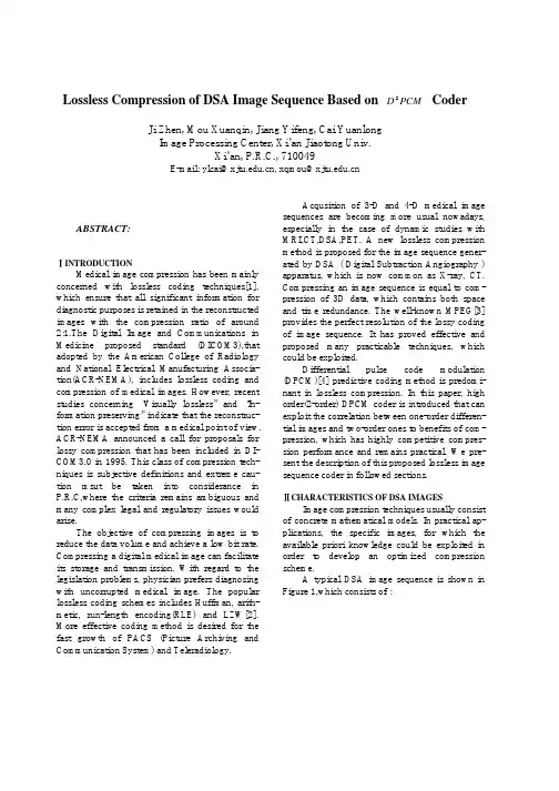
Lossless Compression of DSA Image Sequence Based on PCMD2 CoderJi Zhen, Mou Xuanqin, Jiang Yifeng, Cai YuanlongImage Processing Center, Xi’an Jiaotong Univ.Xi’an, P.R.C., 710049E-mail:**************.cn,**************.cnABSTRACT:ⅠINTRODUCTIONMedical image compression has been mainly concerned with lossless coding techniques[1], which ensure that all significant information for diagnostic purposes is retained in the reconstructed images with the compression ratio of around 2:1.The Digital Image and Communications in Medicine proposed standard (DICOM3),that adopted by the American College of Radiology and National Electrical Manufacturing Associa-tion(ACR-NEMA), includes lossless coding and compression of medical images. However, recent studies concerning “Visually lossless” and “In-formation preserving” indicate that the reconstruc-tion error is accepted from a medical point of view. ACR-NEMA announced a call for proposals for lossy compression that has been included in DI-COM3.0 in 1995. This class of compression tech-niques is subjective definitions and extreme cau-tion msut be taken into considerance in P.R.C,where the criteria remains ambiguous and many complex legal and regulatory issues would arise.The objective of compressing images is to reduce the data volume and achieve a low bit rate. Compressing a digital medical image can facilitate its storage and transmission. With regard to the legislation problems, physician prefers diagnosing with uncorrupted medical image. The popular lossless coding schemes includes Huffman, arith-metic, run-length encoding(RLE) and LZW[2]. More effective coding method is desired for the fast growth of PACS (Picture Archiving and Communication System) and Teleradiology.Acqusition of 3-D and 4-D medical image sequences are becoming more usual nowadays, especially in the case of dynamic studies with MRI,CT,DSA,PET. A new lossless compression method is proposed for the image sequence gener-ated by DSA ( Digital Subtraction Angiography ) apparatus, which is now common as X-ray, CT. Compressing an image sequence is equal to com-pression of 3D data, which contains both space and time redundance. The well-known MPEG[3] provides the perfect resolution of the lossy codingof image sequence. It has proved effective and proposed many practicable techniques, which could be exploited.Differential pulse code modulation (DPCM)[4] predictive coding method is predomi-nant in lossless compression. In this paper, high order(2-order) DPCM coder is introduced that can exploit the correlation between one-order differen-tial images and two-order ones to benefits of com-pression, which has highly competitive compres-sion performance and remains practical. We pre-sent the description of this proposed lossless image sequence coder in followed sections.ⅡCHARACTERISTICS OF DSA IMAGESImage compression techniques usually consistof concrete mathematical models. In practical ap-plications, the specific images, for which the available priori knowledge could be exploited in order to develop an optimized compression scheme.A typical DSA image sequence is shown in Figure 1,which consists of :Figure 1. a typical DSA image sequence (a) M represents mask image, acquired before in-travenous or intraarterious injection. (b) L(n) means the sequence of live images, acquired after intravenous or intraarterious injection. N is the volume of the whole sequence. (c) S(n) is the sub-traction image. S(n)=L(n)-M (n=0,…,N-1).(d) SD(n) is the differential subtraction image. SD(n)=S(n)-S(n-1) (n=1,…,N-1). It is obvious that the whole sequence could be repre-sented in three equivalent formats: Format 1. M and L(n); Format 2. M and S(n);Format 3. M 、S(0) and SD(n).Firstly, the entropy of whole images is calcu-lated separately, H x pp jj j()log ,=−∑ (p jmeans the probability of the jth gray in a image). The followed table could be acquired. In this table. The image resolution is 1024*1024*10bits. Table 1Image H(x) M 6.65 L(n) 6.61 S(n) 4.68 SD(n) 3.67Secondly, the correlation between two images is defined as {})()()(k n I n I E k R +⋅=. We separately obtain the correlation of S(n) and SD(n). The correlation between S(n) is shown in Figure 2(a) and between SD(n) is in (b).From the above curve, followed conclusions about the characteristic of DSA images could be made:(a) when K<5, the correlation R(k) between S(n) often remains very high.(b) the correlation R(k) in SD(n) decreases quickly while K increases. However, the R(1) could hold 0.60, which is useful and important in the pro-posed compression method.Since the three represent formats are equivalent in the mathematical mean, compressing the whole sequence could be implemented in three ways, which would take use of different tech-niques and get different results. It is evident that compression result would better by adopting the last represent than two others because of followed reasons: 1.the entropy is smallest, which mean that the highest lossless compression ratio is prospec-tive theoretically. 2.the R(k) of common signal decreases distinctly after applying one-order dif-ferential, Which means that the two-order differ-ential operation seems worthless. However, it is not the same for the DSA images. The correlation between S(n) holds high, which results in the cer-tain meanness of two-order differential images SD(n). The compression performance would be improved by taking the full advantage of this characteristic.Ⅲ COMPRESSION FRAMEWORK A. Differential Pulse Code ModulationDifferential pulse code modulation(DPCM) exploits the property that the values of adjacent pixels in an image are often similar and highly correlated. The general block diagram of DPCM is shown in Figure 3.The value of a pixel is predictedas a linear combination of a few neighbor pixel values, which is represented as follows: ∑∈−−=Rj i r e n j m i X n m X ),(),(),(αwhere e X is the predicted value, R meansa. R(k) between S(n)b. R(k) between SD(n)Figure 2. the R(k) curve of S(n) and SD(n)xEncoderDecoderneighbor region, ),(n m αare prediction coeffi-cients specified by the image characteristic. Theprediction error defined as ),(),(),(j i X j i X j i e e−= is then coded and trans-mitted. The Decoder reconstructs the pixels as ),(),(j i e j i X X q e r +=In order to keep lossless compression, only thepredictor would be included in DPCM coder. It isa “Predictor + Entropy Coder” lossless DPCMcoding .[5]B. Two Order Differential Pulse Code ModulationThe D PCM 2 coder is different from thetwo-demensional(2-D)DPCM method andthree-demensional(3-D) one[6].For a pixel ),,(j i n X in S(n), applying the DPCM withthe variable n indicates the its extension ofthree-dimension. The same is for the SD(n,x,y) in Format 3, which means two order differential be-cause SD(n) is derived from one differential op-eration oneself. The D PCM 2 coder includes four steps:1.For the mask image M, apply the RICE[7]coding method.2.Construct an optimal predictor. The ARMR model is adopted according to the image attribute. The equation is : )()1,1()1,1(),1()0,1()1,()1,0(e r X X b n m Xr n m Xr n m Xr X −+−−+−+−=αααThe last component of right part means the two-order differential and there is not quantization er-rors.3.For the every pixel S(n,x,y) in S(n), apply to the linear prediction with the variable n.4.Apply adaptive arithmetic algorithm to the error signal ),,(y x n e p . The whole coding process is shown in Figure4.Figure 4. the scheme of D PCM 2coding The dash rectangle constitute the D PCM 2 lossless coder. The decoding process is obvious . Ⅳ EXPERIMENTAL STUDY Figure 5 shows typical DSA images acquiredin Forth Military Medical Univ. of P.R.C. The fig-ure gives the image M, L(60),S(60),S(59) and SD(60) separately. The compression results through this pro-posed method are given as follows: average image size after compression is 463Kbyte. average compression ratio cr ==102410241046364782261***.:average bit rate pixel bit B /42.41024*10248*579338== average compression efficiency η===H x B ()..44236783% The followed table gives the compari-son with Huffman,Arithmetic and DPCM. The compression procedure is equivalent to still image compression without reducing the correlation between images.Huffman Arithmetic DPCM D PCM2Cr 1.36:1 1.47:1 1.53:1 2.26:1 B7.35 6.76 6.76 4.42From above table, it is obvious that this proposed compression technique performs better than others.ⅤCONCLUSIONWith applying the proposed method to the DSA apparatus, perfect experiment performance is deserved. The compression ratio is better than or-dinary techniques. The computational time and space also prove practicable and robust. Although significant progress Many researches remain.ACKNOWLEDGMENTThe authors wish to thank Dr.Sun Li-jun,FMMU for his cooperation on acquisition of some important DSA images.(a) M (b) L(60)(c) S(60) (d) S(59) (e) SD(60)(enhancement for display)Figure 5. (a) mask image (b) live image (c)and (d) subtraction image (e) differential subtraction image1.S.Wong, L.Zaremba.D.Gooden,and H.K.Huang. “Radiologic image compression-A Reivew”,Proc. IEEE,vol,83,pp194-219,Feb.1995.2.A.K.Jain, Fundamentals of Digital Image Processing. Eaglewood Cliffs,NJ:Prentice-Hall,1989.3.MPEG(ISO/IEC JTC1/SC29/WG11).Coding of Moving Pictures and Associated Audio for Digital Storage Media at up to 1.5MBit/s ISO.CD 11172,Nov,1991.4.G.Bostelmann,“A simple high quality DPCM-Codec for video telephony using 8 Mbit per sec-ond”,NTZ,27(3),pp115-117,1974.5.L.N.Wu, Data Compression & Application, Electrical Industry Publisher,pp116-120,19956.P.Roos and M.A.Viegever, “Reversible 3_D decorrelation of medical images”, IEEE, Medical Im-aging,12(3),pp413-420,1993.7.D.Yeh, ler, “The development of lossless data compression technology for remote sensing application”, pp307-309,In IGRASS’94.。

改进Retinex⁃Net的低光照图像增强算法欧嘉敏1 胡　晓1 杨佳信1摘　要　针对Retinex⁃Net存在噪声较大㊁颜色失真的问题,基于Retinex⁃Net的分解-增强架构,文中提出改进Ret⁃inex⁃Net的低光照图像增强算法.首先,设计由浅层上下采样结构组成的分解网络,将输入图像分解为反射分量与光照分量,在此过程加入去噪损失,抑制分解过程产生的噪声.然后,在增强网络中引入注意力机制模块和颜色损失,旨在增强光照分量亮度的同时减少颜色失真.最后,反射分量和增强后的光照分量融合成正常光照图像输出.实验表明,文中算法在有效提升图像亮度的同时降低增强图像噪声.关键词　低光照图像增强,深度网络,视网膜大脑皮层网络(Retinex⁃Net),浅层上下采样结构,注意机制模块引用格式　欧嘉敏,胡晓,杨佳信.改进Retinex⁃Net的低光照图像增强算法.模式识别与人工智能,2021,34(1):77-86.DOI　10.16451/ki.issn1003⁃6059.202101008 中图法分类号　TP391.4Low⁃Light Image Enhancement Algorithm Based onImproved Retinex⁃NetOU Jiamin1,HU Xiao1,YANG Jiaxin1ABSTRACT　Aiming at the problems of high noise and color distortion in Retinex⁃Net algorithm,a low⁃light image enhancement algorithm based on improved Retinex⁃Net is proposed grounded on the decomposition⁃enhancement framework of Retinex⁃Net.Firstly,a decomposition network composed of shallow upper and lower sampling structure is designed to decompose the input image into reflection component and illumination component.In this process,the denoising loss is added to suppress the noise generated during the decomposition process.Secondly,the attention mechanism module and color loss are introduced into the enhancement network to enhance the brightness of the illumination component and meanwhile reduce the image color distortion.Finally,the reflection component and the enhanced illumination component are fused into the normal illumination image to output.The experimental results show that the proposed algorithm improves the image brightness effectively with the noise of enhanced image reduced.Key Words　Low⁃Light Image Enhancement,Deep Network,Retinal Cortex Theory⁃Net,Shallow Up⁃per and Lower Sampling Structure,Attention Mechanism ModuleCitation　OU J M,HU X,YANG J X.Low⁃Light Image Enhancement Algorithm Based on Improved Retinex⁃Net.Pattern Recognition and Artificial Intelligence,2021,34(1):77-86.收稿日期:2020-05-12;录用日期:2020-09-17 Manuscript received May12,2020;accepted September17,2020国家自然科学基金项目(No.62076075)资助Supported by National Natural Science Foundation of China(No. 62076075)本文责任编委黄华Recommended by Associate Editor HUANG Hua1.广州大学电子与通信工程学院　广州5100061.School of Electronics and Communication Engineering,Guang⁃zhou University,Guangzhou510006 由于低光照环境和有限的摄像设备,图像存在亮度较低㊁对比度较低㊁噪声较大㊁颜色失真等问题,不仅会影响图像的美学㊁人类的视觉感受,还会降低运用正常光照图像的高级视觉任务的性能[1-3].为了有效改善低光图像质量,学者们提出许多低光照图像增强算法,经历灰度变换[4-5]㊁视网膜皮层理论[6-11]和深度神经网络[12-19]三个阶段.早期,通过直方图均衡[4-5]㊁伽马校正等灰度变换方法对低亮度区域进行灰度拉抻,可达到提高暗区亮度的目的.然而,因为未考虑像素与其邻域像素的关系,灰度变换常会导致增强图像缺乏真实感.第34卷　第1期模式识别与人工智能Vol.34　No.1 2021年1月Pattern Recognition and Artificial Intelligence Jan.　2021Land [6]提出视网膜皮层理论(Retinal CortexTheory,Retinex).该理论认为物体颜色与光照强度无关,即物体具有颜色恒常性.基于该理论,相继出现经典的单尺度视网膜增强算法(Single Scale Retinex,SSR)[7]和色彩恢复的多尺度视网膜增强算法(Multi⁃scale Retinex with Color Restoration,MSR⁃CR)[8].算法主要思想是利用高斯滤波器获取低光照图像的光照分量,再通过像素间逐点操作求得反射分量作为增强结果.Wang 等[9]利用亮通滤波器和对数变换平衡图像亮度和自然性,使增强后的图像趋于自然.Fu 等[10]设计用于同时估计反射和光照分量(Simultaneous Reflectance and Illumination Esti⁃mation,SRIE)的加权变分模型,可有效处理暗区过度增强的问题.Guo 等[11]提出仅估计光照分量的低光照图像增强算法(Low Light Image Enhancementvia Illumination Map Estimation,LIME),主要利用局部一致性和结构感知约束条件计算图像的反射分量并作为输出结果.然而,这些基于Retinex 理论模型的算法虽然可调整低光图像亮度,但增亮程度有限.研究者发现卷积神经网络(Convolutional NeuralNetwork,CNN)[12]与Retinex 理论结合能进一步提高增强图像的视觉效果,自动学习图像的特征,解决Retinex 依赖手工设置参数的问题.Lore 等[13]提出深度自编码自然低光图像增强算法(A Deep Auto⁃encoder Approach to Natural Low Light Image Enhan⁃cement,LLNet),有效完成低光增强任务.Lü等[14]提出多边低光增强网络(Multi⁃branch Low⁃Light En⁃hancement Network,MBLLEN),学习低光图像到正常光照图像的映射.Zhang 等[15]结合最大信息熵和Retinex 理论,提出自监督的光照增强网络.Wei 等[16]基于图像分解思想,设计视网膜大脑皮层网络(Retinex⁃Net),利用分解-增强架构调整图像亮度.Zhang 等[17]基于Retinex⁃Net 设计低光增强器.然而,由于噪声与光照水平有关,Retinex⁃Net 提取反射分量后,图像暗区噪声高于亮区.因此,Retinex⁃Net 的增强结果存在噪声较大㊁颜色失真的问题,不利于图像质量的提升.为此本文提出改进Retinex⁃Net 的低光照图像增强算法.以Retinex⁃Net 的分解与增强框架为基础,针对噪声问题,在分解网络采用浅层上下采样结构[15],利用反射分量梯度项[15]作为损失.同时为了改善增强图像的色彩偏差,保留丰富的细节信息,在增强网络中嵌入注意力机制模块[18]和颜色损失[19].实验表明,本文算法在LOL 数据集和其它公开数据集上取得较优的视觉效果和客观结果.1　改进Retinex⁃Net 的低光照图像增强算法改进Retinex⁃Net 的低光照图像增强算法框图如图1所示.S lowS normalR highI highI lowR lowI end图1　本文算法框图Fig.1　Flowchart of the proposed algorithm87模式识别与人工智能(PR&AI) 第34卷 Retinex理论[6]认为彩色图像可分解为反射分量和光照分量:S=R I.(1)其中: 表示逐像素相乘操作;S表示彩色图像,可以是任何具有不同曝光程度的图像;R表示反射分量,反映物体内在固有属性,与外界光照无关;I表示光照分量,不同曝光度的物体光照分量不同.本文算法主要利用2个相互独立训练的子网络,分别是分解网络与增强网络.具体地说,首先,分解网络以数据驱动方式学习,将低光照图像和与之配对的正常光照图像分解为相应的反射分量(R low, R normal)和光照分量(I low,I normal).然后,增强网络以低光图像的光照分量I low作为输入,在结构感知约束下,提升光照分量的亮度.最后,重新组合增强的光照分量I en与反射分量R low,形成增强图像S en,作为网络输出.1.1　分解网络的浅层上下采样结构由于式(1)是一个不适定问题[20],很难设计适用于多场景的约束函数.本文算法以数据驱动的方式进行学习,不仅能解决该问题,还能进一步提高网络的泛化能力.如图1所示,在训练阶段,分解网络以低光照图像S low和与之对应的正常光照图像S normal 作为输入,在约束条件下学习输出它们一致的反射分量R low和R normal,及不同的光照分量I low和I normal.值得注意的是,S low与S normal共享分解网络的参数.区别于常用的深度U型网络(U⁃Net)结构及Retinex⁃Net简单的堆叠卷积层,本文算法的分解网络是一个浅层的上下采样结构,由卷积层与通道级联操作组成,采样层只有4层,网络训练更简单.实验表明,运用此上下采样结构变换图像尺度时,下采样操作一定程度上舍去含有噪声的像素点,达到降噪效果的目的,但同时会引起图像的模糊.因此为了提高分解图像清晰度,减少语义特征丢失,在图像上采样后应用通道数级联操作,可给图像补偿下采样丢失的细节信息,增强清晰度.在浅层上下采样结构中,首先,使用1个9×9的卷积层提取输入图像S low的特征.然后,采用5层以ReLU作为激活函数的卷积层变换图像尺度,学习反射分量与光照分量的特征.最后,分别利用2层卷积层及Sigmoid函数,将学习到的特征映射成反射图R low和光照图I low后再输出.对于分解网络的约束损失,本文算法沿用Retinex⁃Net的重构损失l rcon㊁不变反射率损失l R及光照平滑损失l I.另外为了在分解网络中更进一步减小噪声,添加去噪损失l d.因此总损失如下:l=l rcon+λ1l R+λ2l I+λ3l d,其中,λ1㊁λ2㊁λ3为权重系数,用于平衡各损失分量.对于L1㊁L2范数和结构相似性(Structural Similarity, SSIM)损失的选择,当涉及图像质量任务时,L2范数与人类视觉对图像质量的感知没有很好的相关性,在训练中容易陷入局部最小值,而SSIM虽然能较好地学习图像结构特征,但对平滑区域的误差敏感度较低,引起颜色偏差[21].因此本文算法使用L1范数约束所有损失.在分解网络中输出的结果R low和R normal都可与光照图重构成新的图像,则重构损失如下:l rcon=∑i=low,normalW1Rlow I i-S i1+∑j=low,normal W2R normal I j-S j1,其中 表示逐像素相乘操作.当i为low或j为normal 时,权重系数W1=W2=1,否则W1=W2=0.001.对于配对的图像,使用较大的权重能够使分解网络更好地学习配对图像的特征.对于配对的图像对,使用较大的权重可使分解网络更好地学习配对图像的特征.不变反射率损失l R是基于Retinex理论的颜色恒常性,在分解网络中主要用于约束学习不同光照图像的一致反射率:l R=Rlow-R normal1.对于光照平滑损失l I,本文采用结构感知平滑损失[16].该损失以反射分量梯度项作为权重,在图像梯度变化较大的区域,光照变得不连续,从而亮度平滑的光照图能保留图像结构信息,则l I=ΔIlow exp(-λgΔR low)1+ΔI normal exp(-λgΔR normal)1,其中,Δ表示图像水平和垂直梯度和,λg表示平衡系数.Rudin等[22]观察到,噪声图像的总变分(Total Variation,TV)大于无噪图像,通过限制TV可降低图像噪声.然而在图像增强中,限制TV相当于最小化梯度项.受TV最小化理论[22-23]启发,本文引入反射分量的梯度项作为损失,用于控制反射图像噪声,故称为去噪损失:l d=λΔRlow1.当λ值增加时,噪声减小,同时图像会模糊.因此对于权重参数的选择十分重要,经过实验研究发现,当权重λ=0.001时,图像获得较好的视觉效果.1.2　增强网络的注意力机制如图1所示,增强网络以分解网络的输出I low作97第1期 欧嘉敏　等:改进Retinex⁃Net的低光照图像增强算法为输入,学习增强I low的亮度,将增强结果I en与分解网络另一输出R low重新结合为增强图像S en后输出.在增强网络中,I low经过多个下采样块生成较小尺度图像,使增强网络有较大尺度角度分配光照,从而具有调节亮度的能力.网络采用上采样方式重构局部光照,对亮的区域分配较低亮度,对较暗的区域调整较高亮度.此外,将上采样层的输出进行通道数的级联,在调整不同局部光照的同时,保持全局光照一致性.而且跳过连接是从下采样块引入相应的上采样块,通过元素求和,强制网络学习残差.针对Retinex⁃Net出现的颜色失真问题,在增强网络中嵌入注意力机制模块.值得注意的是,与其它复杂的注意力模块不同,注意力机制模块由简单卷积层和激活操作组成,不要求强大的硬件设备,也不需要训练多个模型和大量额外参数.在光照调整过程中,可减少对无关背景的特征响应,只激活感兴趣的特征,提高算法对图像细节的处理能力和对像素的敏感性,指导网络既调整图像亮度又保留图像结构.由图1可见,注意力模块的输入是图像特征αi㊁βi,输出为图像特征γi,i=1,2,3,表示注意力机制模块的序号.αi为下采样层输出的图像特征,βi为上采样层的输出特征.这2个图像特征分别携带不同的亮度信息,两者经过注意力模块后,降低亮度无关特征(如噪声)的响应,使输出特征γi携带更多亮度信息被输入到下一上采样层,提高网络对亮度特征的学习能力.αi与重建尺度后的βi分别经过一个独立的1×1卷积层,在ReLU激活之前进行加性操作.依次经过1×1卷积层㊁Sigmoid函数,最后与βi通过逐元素相乘后将结果与αi进行通道级联.在此传播过程中,注意机制可融合不同尺度图像信息,同时减少无关特征的响应,增强网络调整亮度能力.独立于分解网络的约束损失,增强网络调整光照程度是基于局部一致性和结构感知[16]的假设.本文算法除了沿用Retinex⁃Net中约束增强网络的损失外,在实验中,针对Retinex⁃Net出现的色彩偏差,增加颜色损失[19],因此增强网络损失:L=L rcon+L I+μL c,其中,L rcon为增强图像的重构损失,L rcon=Snormal-R low I en1,L I表示结构感知平滑损失,L c表示本文的颜色损失,μ表示平衡系数.L rcon定义表示增强后的图像与其对应的正常光照图像的距离项,结构感知平滑损失L I 与分解网络的平滑损失类似,不同的是,在增强网络中,I en以R low的梯度作为权重系数:L I=ΔIen exp(-λgΔR low)1.此外,本文添加颜色损失L c,衡量增强图像与正常光照图像的颜色差异.先对2幅图像采用高斯模糊,滤除图像的纹理㊁结构等高频信息,留下颜色㊁亮度等低频部分.再计算模糊后图像的均方误差.模糊操作可使网络在限制纹理细节干扰情况下,更准确地衡量图像颜色差异,进一步学习颜色补偿.颜色损失为L c=F(Sen)-F(S normal)21.其中:F(x)表示高斯模糊操作,x表示待模糊的图像.该操作可理解为图像每个像素以正态分布权重取邻域像素的平均值,从而达到模糊的效果,S en为增强图像,S normal为对应的正常光照图像,F(x(i,j))=∑k,lx(i+k,j+l)G(k,l),G(k,l)表示服从正态分布的权重系数.在卷积网络中G(k,l)相当于固定大小的卷积核,G(k,l)=0.æèçç053exp k2-l2öø÷÷6.2　实验及结果分析2.1　实验环境本文算法采用LOL训练集[16]和合成数据集[16]训练网络.测试集选取LOL的评估集㊁DICM数据集㊁MEF数据集.在训练过程中,网络采用图像对训练,批量化大小(Batch Size)设为32,块大小(Patch Size)设为48×48.分解网络的损失平衡系数λ1=0.001,λ2=0.1,λ3=0.001.增强网络的平衡系数μ=0.01,λg=10.本文采用自适应矩估计优化器(Adaptive Moment Estima⁃tion,Adam).网络的训练和测试实验均在Nvidia GTX2080GPU设备上完成,实现代码基于TensorFlow框架.为了验证本文算法的性能及效果,采用如下对比算法:Retinex⁃Net,SRIE[10],LIME[11],MBLLEN[14]㊁文献[15]算法㊁全局光照感知和细节保持网络(Global Illumination⁃Aware and Detail⁃Preserving Net⁃work,GLADNet)[24]㊁无成对监督深度亮度增强(Deep Light Enhancement without Paired Supervision, EnlightenGAN)[25].在实验过程中,均采用原文献提供的模型或源代码对图像进行测试.采用如下客观评估指标:峰值信噪比(Peak Signal to Noise Ratio,PSNR)㊁结构相似性(Structural08模式识别与人工智能(PR&AI) 第34卷Similarity,SSIM)[26]㊁自然图像质量评估(NaturalQuality Evaluator,NIQE)[27]㊁通用图像质量评估(Universal Quality Index,UQI)[28]㊁基于感知的图像质量评估(Perception⁃Based Image Quality Evaluator,PIQE)[29].SSIM㊁PSNR㊁UQI 值越高,表示增强结果图质量越优.相反,PIQE㊁NIQE 值越高,表示图像质量越差.2.2　消融性实验为了进一步验证本文算法各模块的有效性,以Retinex⁃Net 为基础设计消融性实验,利用PSNR 衡量噪声水平,采用SSIM 从亮度㊁对比度㊁结构评估图像综合质量.实验结果如表1所示,表中S⁃ULS 表示浅层上下采样结构,l d 表示去噪损失.Enhan _I low 表示增强网络输入仅为光照分量,AMM 表示注意力机制模块,L c 表示颜色损失.参数微调1表示增强网络的平滑损失系数由原Retinex⁃Net 的3设为1;参数微调2是增强网络的平滑损失系数为1,批量化大小由16设为32.表1　各改进模块及损失的消融性实验结果Table 1　Ablation experiment results of improved modules and loss序号基础框架改进方法PSNRSSIM1-Retinex⁃Net 16.7740.55923Retinex⁃Net 添加S⁃ULS,不添加l d 添加S⁃ULS,添加l d17.45217.4940.6890.699456Retinex⁃Net+S⁃ULS+l d添加Enhan _I low ,不添加AMM,不添加L c 添加Enhan _I low ,添加AMM,不添加L c 添加Enhan _I low ,添加AMM,添加L c17.89718.00218.0910.7030.7080.70478Retinex⁃Net+S⁃ULS+l d +AMM+L c参数微调1参数微调218.27218.5290.7190.720 表1中序号2给出以Retinex⁃Net 为基础,采用浅层上下采样结构作为分解网络的结果.相比Retinex⁃Net,PSNR 值显著提高,表明此结构可抑制由图像分解带来的噪声.在此基础上添加去噪损失,进一步降低噪声,见序号3.由此验证浅层上下采样结构与去噪损失的有效性.在本文算法中,由于采用两步训练的方式,即先训练分解网络后训练增强网络,因此在验证浅层上下采样结构和去噪损失的有效性后,以此为基础评估增强网络引入的注意力机制模块和颜色损失的有效性.在Retinex⁃Net 中增强网络的输入为反射分量与光照分量通道级联后的结果.该设置一定程度上会导致反射分量丢失图像结构和细节,同时影响光照分量的亮度提升.为此,先设置序号4的实验验证上述分析.由结果可见:PSNR㊁SSIM 值大幅提高,证明此分析的正确性,表明本文算法的增强网络仅以光照分量作为输入的有效性.另外,从序号5结果看出,利用注意力模块后,图像噪声显著降低,这归功于注意力模块可减少对图像无关特征的响应,集中注意力学习亮度特征,从而降低图像噪声水平.在颜色损失的消融性实验中,尽管客观数值上没有直观体现颜色的恢复,但根据图2和图3可知,该损失是有效的.为了使各模块更好地发挥优势,本文算法对参数进行微调.从序号7㊁序号8的实验结果可见,微调参数后本文算法各模块作用进一步体现,取得更优结果. (a)输入图像 (b)参考图像 (a)Input image (b)Ground truth18第1期 欧嘉敏　等:改进Retinex⁃Net 的低光照图像增强算法 (c)SRIE (d)LIME (e)GLADNet (f)MBLLEN (g)EnlightenGAN (h)Retinex⁃Net (i)文献[15]算法 (j)本文算法 (i)Algorithm in reference[15]　(j)The proposed algorithm图2　各算法在LOL数据集上的视觉效果Fig.2　Visual results of different algorithms on LOLdatasetA B C D(a)输入图像(a)Inputimages(b)LIME(c)GLADNet28模式识别与人工智能(PR&AI) 第34卷(d)MBLLEN(e)EnlightenGAN(f)Retinex⁃Net(g)文献[15]算法(g)Algorithm in reference[15](h)本文算法(h)The proposed algorithm图3　各算法在DICM㊁MEF数据集上的视觉效果Fig.3　Visual results of different algorithms on DICM and MEF datasets38第1期 欧嘉敏　等:改进Retinex⁃Net的低光照图像增强算法2.3　对比实验各算法在3个数据集上的客观评估结果如表2所示,表中黑体数字表示最优结果,斜体数字表示次优结果.在LOL 数据集上,SSIM 可从亮度㊁对比度㊁结构度量2幅图像相似度,与人类视觉系统(Human Vision System,HVS)具有较高相关性[21,30],可较全面体现图像质量.从表2可见,在SSIM㊁UQI 指标上,本文算法取得最高数值,表明低光照图像经本文算法增强后图像质量得到明显提升.从图2和图3发现,本文算法也提升视觉效果的表现力.由表2的LOL 数据集上结果可知,在PSNR 指标上,本文算法总体上优于先进算法.根据文献[21]㊁文献[30]和文献[31]的研究,PSNR 指标因为容易计算,被广泛用于评估图像,但其计算是基于误差敏感度,在评估中常出现与人类感知系统不一致的现象,因此与图像主观效果结合分析能更好地体现图像质量.结合图2和图3的分析,GLADNet 的增强图像饱和度较低,存在颜色失真现象.文献[15]算法使图像过曝光.本文算法在Retinex⁃Net 基础上显著降低图像噪声,保留图像丰富结构信息,相比其它方法,视觉效果更佳,符合人类的视觉感知系统.在LOL 数据集上,对比大部分算法,本文取得与参考图像相近的NIQE 数值,表明本文算法的增强结果更接近参考图像.DICM㊁MEF 数据集没有正常光照图作为参照.本文只采用盲图像质量评估指标(NIQE㊁PIQE)评估各算法.在PIQE 指标上,本文算法取得最优值.对于NIQE,虽然未取得较好优势,但相比Retinex⁃Net,本文算法取得更好的增强结果.综上所述,虽然本文算法未在所有指标上取得最优结果,但仍有较高优势.在与人类视觉感知系统有较好相关性的SSIM 指标及噪声抑制和避免过曝能力上,本文算法最优.表2　各算法在3个数据集上的客观评估结果Table 2　Objective evaluation results of different algorithms on 3datasets 算法LOL 数据集SSIMUQI PSNRNIQEDICM 数据集PIQE NIQEMEF 数据集PIQE NIQESRIE0.4980.48211.8557.28716.95 3.89810.70 3.474LIME 0.6010.78916.8348.37815.60 3.8319.12 3.716GLADNet 0.7030.87919.718 6.47514.85 3.6817.96 3.360MBLLEN0.7040.82517.5633.58412.293.27012.043.322EnlightenGAN 0.6580.80817.483 4.68414.613.5627.863.221文献[15]算法0.7120.86019.150 4.79316.21 4.71811.78 4.361Retinex⁃Net 0.5590.87916.7749.73014.16 4.41511.90 4.480本文算法0.7200.88018.5294.49010.11 3.9607.77 3.820参考图像1--4.253---- 由图2可见,SRIE㊁LIME㊁EnlightenGAN 的增亮程度有限,增强结果偏暗.GLADNet㊁MBLLEN 改变图像饱和度,降低图像视觉效果.相比Retinex⁃Net,本文算法的增强结果图噪声水平较低,可保持图像原有的色彩.由图3可见,SRIE 增强程度远不足人类视觉需求,在图3的图像A 中,未展示其增强结果.在图3中,根据人眼视觉系统,首先能判断LIME㊁GLADNet㊁MBLLEN㊁EnlightenGAN 对人脸的增亮程度仍不足,GLADNet㊁MBLLEN 分别存在饱和度过低和过高现象.而文献[15]算法㊁Retinex⁃Net㊁本文算法能较好观察到人脸细节,但同时从左下角细节图可见,Retinex⁃Net 人脸的边缘轮廓对比度过强.从颜色上进一步分析可知,文献[15]算法亮度过度增强,导致图像颜色失真,如天空的颜色对比输入图像色调偏白㊁曝光难以观察远处的景物等.同样观察图3中图像B 右下角细节,经过分析可得,文献[15]算法㊁Retinex⁃Net㊁本文算法增强程度满足人类视觉需求,但文献[15]算法过曝光,从Retinex⁃Net 细节图可见人物服饰失真.对比其它算法,本文算法结果的亮度适中,图像具有丰富细节,避免光照伪影与过曝光现象.另外,从图3中图像C㊁D 可见,LIME㊁GLAD⁃Net㊁MBLLEN㊁EnlightenGAN 没能较好处理局部暗48模式识别与人工智能(PR&AI) 第34卷区,如笔记本㊁右下角拱门窗户区域仍未增亮,导致难以识别边缘细节.而文献[15]算法饱和度发生变化.Retinex⁃Net存在伪影和噪声等问题.本文算法不仅可增强图像的亮度,减小噪声,还保留图像的细节,图像效果更有利于高级视觉系统的识别或检测.综合上述分析发现,本文算法对低光照图像增强效果更优.3　结束语针对Retinex⁃Net噪声较大㊁颜色失真问题,本文提出改进Retinex⁃Net的低光照图像增强算法.算法在分解网络采用浅层上下采样结构及去噪损失,在增强网络嵌入注意力机制模块和颜色损失.实验表明,本文算法不仅能增强图像亮度,而且能显著降低噪声,并取得较优结果.本文算法较好地处理亮度增强过程中无法避免的噪声问题,兼顾提升亮度和降低噪声任务,可给未来研究图像多属性增强提供思路,如低光增强㊁去噪㊁颜色恢复㊁去模糊等多任务同步进行.今后研究重心将是实现图像多属性同步增强.同时扩展该研究网络结构到其它高级视觉任务中,作为图像预处理模块,期望实现网络的端到端训练.参考文献[1]HU X,MA P R,MAI Z H,et al.Face Hallucination from Low Quality Images Using Definition⁃Scalable Inference.Pattern Reco⁃gnition,2019,94:110-121.[2]陈琴,朱磊,后云龙,等.基于深度中心邻域金字塔结构的显著目标检测.模式识别与人工智能,2020,33(6):496-506. (CHEN Q,ZHU L,HOU Y L,et al.Salient Object Detection Based on Deep Center⁃Surround Pyramid.Pattern Recognition and Artificial Intelligence,2020,33(6):496-506.)[3]杨兴明,范楼苗.基于区域特征融合网络的群组行为识别.模式识别与人工智能,2019,32(12):1116-1121. (YANG X M,FAN L M.Group Activity Recognition Based on Re⁃gional Feature Fusion Network.Pattern Recognition and Artificial Intelligence,2019,32(12):1116-1121.)[4]CHENG H D,SHI X J.A Simple and Effective Histogram Equaliza⁃tion Approach to Image Enhancement.Digital Signal Processing, 2004,14(2):158-170.[5]ABDULLAH⁃AI⁃WADUD M,KABIR M H,DEWAN M A A,et al.A Dynamic Histogram Equalization for Image Contrast Enhancement. IEEE Transactions on Consumer Electronics,2007,53(2):593-600.[6]LAND E H.The Retinex Theory of Color Vision.Scientific Ameri⁃can,1977,237(6):108-128.[7]JOBSON D J,RAHMAN Z,WOODELL G A.Properties and Per⁃formance of a Center/Surround Retinex.IEEE Transactions on Im⁃age Processing,1997,6(3):451-462.[8]JOBSON D J,RAHMAN Z,WOODELL G A.A Multiscale Retinex for Bridging the Gap between Color Images and the Human Observa⁃tion of Scenes.IEEE Transactions on Image Processing,1997, 6(7):965-976.[9]WANG S H,ZHENG J,HU H M,et al.Naturalness Preserved En⁃hancement Algorithm for Non⁃uniform Illumination Images.IEEE Transactions on Image Processing,2013,22(9):3538-3548.[10]FU X Y,ZENG D L,HUANG Y,et al.A Weighted VariationalModel for Simultaneous Reflectance and Illumination Estimation// Proc of the IEEE Conference on Computer Vision and Pattern Re⁃cognition.Washington,USA:IEEE,2016:2782-2790. [11]GUO X J,LI Y,LING H B.LIME:Low⁃Light Image Enhance⁃ment via Illumination Map Estimation.IEEE Transactions on Image Processing,2017,26(2):982-993.[12]FUKUSHIMA K.Neocognitron:A Self⁃organizing Neural NetworkModel for a Mechanism of Pattern Recognition Unaffected by Shift in Position.Biological Cybernetics,1980,36:193-202. [13]LORE K G,AKINTAYO A,SARKAR S.LLNet:A Deep Autoen⁃coder Approach to Natural Low⁃Light Image Enhancement.Pattern Recognition,2017,61:650-662.[14]LÜF F,LU F,WU J H,LIM C S.MBLLEN:Low⁃Light Image/Video Enhancement Using CNNs[C/OL].[2020-05-11].http:// /bmvc/2018/contents/papers/0700.pdf. [15]ZHANG Y,DI X G,ZHANG B,et al.Self⁃supervised Image En⁃hancement Network:Training with Low Light Images Only[C/ OL].[2020-05-11].https:///pdf/2002.11300.pdf.[16]WEI C,WANG W J,YANG W H,et al.Deep Retinex Decom⁃position for Low⁃Light Enhancement[C/OL].[2020-05-11].https: ///pdf/1808.04560.pdf.[17]ZHANG Y H,ZHANG J W,GUO X J.Kindling the Darkness:APractical Low⁃Light Image Enhancer//Proc of the27th ACM In⁃ternational Conference on Multimedia.New York,USA:ACM, 2019:1632-1640.[18]AI S,KWON J.Extreme Low⁃Light Image Enhancement for Sur⁃veillance Cameras Using Attention U⁃Net.Sensors,2020,20(2): 495-505.[19]IGNATOV A,KOBYSHEV N,TIMOFTE R,et al.DSLR⁃QualityPhotos on Mobile Devices with Deep Convolutional Networks// Proc of the IEEE International Conference on Computer Vision.Washington,USA:IEEE,2017:3297-3305.[20]TIKHONOV A N,ARSENIN V Y.Solutions of Ill⁃Posed Pro⁃blems.SIAM Review,1979,21(2):266-267. [21]ZHAO H,GALLO O,FROSIO I,et al.Loss Functions for ImageRestoration with Neural Networks.IEEE Transactions on Computa⁃58第1期 欧嘉敏　等:改进Retinex⁃Net的低光照图像增强算法。

2
无损图像认证算法
与罗等[9]的 LIAA 类似，本文提出的基于自适 应分块组合的无损图像认证算法（ALIAA）采用动 态方式确定认证块，认证块划分基本思想是：首先 选定一种适合小尺寸图像块的无损水印算法，由该 无损水印算法和篡改定位精度要求等综合确定图 像基本块 （bb） 的尺寸； 把原图像 I 划分为 m 个 （不 足构成完整基本块的用 0 填充扩展）能够被识别的 基本块 (bbi,1≤i≤m)；m 个 bbi 根据某种规则自适 应地生成 n 个图像认证块(abj,1≤j≤n)。 在划分基本 块和认证块的过程中要求满足以下基本条件。
摘
要：现有基于分块的无损图像认证算法在图像认证块划分方面存在不足。为此，提出一种基于自适应分块组
合的无损图像认证算法。算法中的认证块由基本分块根据原图像特征和水印图像保真度要求自适应组合而成，认 证信息用数字签名技术产生，以无损水印方式嵌入，同时以多次嵌入方式实现图像编号的顽健传送，利用图像编 号和认证块编号防止矢量量化攻击。理论分析与实验结果表明该算法篡改定位能力强于现有无损图像认证算法， 且适应性强，能抗矢量量化攻击。 关键词：无损图像认证；可逆图像认证；无损图像水印；可逆图像水印；篡改定位；矢量量化攻击 中图分类号：TP391 文献标识码：A 文章编号：1000-436X(2012)06-0064-09
Lossless image authentication algorithm based on adaptive combinations of image basic blocks
LUO Jian-gao1, HAN Guo-qiang2, WO Yan2, LI Xiang-yang1
(1. Department of Computer, Guangdong AIB Polytechnic College, Guangzhou 510507, China; 2. School of Computer Science and Engineering, South China University of Technology, Guangzhou 510006, China. )

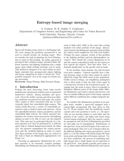
Entropy-based image mergingA.German,M.R.Jenkin,Y.Lesp´e ranceDepartment of Computer Science and Engineering and Centre for Vision Research York University,Toronto,Ontario,Canada.{german,jenkin,lesperan}@cs.yorku.caAbstractSpacecraft docking using vision is a challenging task. Not least among the problems encountered is the need to visually localize the docking target.Here we consider the task of adapting the local illumina-tion to assist in this docking.An online approach is developed that combines images obtained under dif-ferent exposure and lighting conditions into a single image upon which docking decisions can be made. This method is designed to be used within an intel-ligent controller that automatically adjusts lighting and image acquisition in order to obtain the“best”possible composite view of the target for further im-age processing.Keywords:Image Entropy,High Dynamic Range. 1IntroductionPerhaps the most interesting vision tasks involve guiding semi-autonomous vehicles such as unmanned underwater vehicles,mining machines and space-craft.Given the widely varying and often poor light-ing conditions encountered in such tasks,the remote video camera is often associated with one or more (typicallyfixed)but controllable light sources.The camera itself often has a variety of controllable pa-rameters such as shutter speed and aperture.Given the controllable intrinsic camera parameters,and the controllable light sources,the remote operator ma-nipulates the various camera parameters and lighting options in order to be able to carry out the required task.This task may be performed directly by a hu-man operator or it may be performed by a software agent with or without human intervention.In either case,the operator manipulates the camera param-eters and the available lighting in order to ensure that those portions of the image that are critical to the task at hand are illuminated appropriately(see Figure1a).Choosing an appropriate illumination for a hu-man operator is an extremely complex problem. Maximizing one illuminant may place portions of the scene in high relief,while at the same time casting shadows over other portions of the image.Interac-tions between the illuminants and gain control within the camera itself complicates the task even further. Perhaps the most common version of this problem is the lighting problem portrait photographers en-counter:How should the various illuminates be lit and the camera controlled in order for the camera to best capture the subject?Note that what“best”is depends significantly on the specific task on hand.In the machine vision domain,the task becomes even more complex.Cameras typically have a lim-ited dynamic range so they often cannot be used to effectively image the whole scene in one acquisition. Unlike natural settings,one simplifying assumption that is often made is that the only active agent in a teleoperated setting is the teleoperated agent.As-suming that the scene is static,then it is possible to illuminate different parts of the image under differ-ent illuminates and camera capture parameters,and then to combine different parts of the image captured under different conditions into a single composite im-age.To consider this illumination problem in its sim-plest form,consider a spacecraft equipped with a camera-light arrangement like that given in Fig-ure1b.If one assumes that the underlying camera capture and scene geometry is static,i.e.,the space-craft are not moving relative to each other and the position of the camera,the lights and object being viewed remain unchanged,then the camera’s intrin-sic parameters and the level of illumination provided by each light can be manipulated.Furthermore,if the aperture,focus and focal length of the camera re-main unchanged,then over a set of images taken un-der different lighting and camera parameters,a given pixel(u,v)in the camera will always image the same scene point and image blur will remain constant.Un-der these conditions,the process of combining mul-tiple images into a single image can be expressed at the pixel level–how should a specific pixel values at (u,v),taken under different illumination and camera(a)A computer graphics rendering of the space shuttle docking procedure.(b)An intelligent controller can manipulate light-ing intensities and camera intrinsics in order to derive an accurate model of the relationships be-tween the spacecrafts involved in a docking pro-cedure.Figure1:Illumination issues in teleoperation.How can the scene be best illuminated and captured in order to dock the two vehicles?parameters,be combined to obtain a composite pixelvalue at(u,v)?1.1Formal Statement of the ProblemGiven a set of images{I1,...,I N},a functionφis de-sired that combines the set into a single image˜I1...N.Notationally,we seek a functionφ()that operates atthe pixel level and that has the following properties:˜I1=φ(I1)˜I1...N=φ(I1,I2,...,I N)In order for the image merging to operate in an ef-ficient,online mannerφshould have the propertythat˜I1...N+1=φ(˜I1...N,I N+1)That is,it should be efficient to compute the N+1th image of˜I given the computation for the N th image. 2Related WorkThe problem of combining multiple images taken un-der varying sensor/lighting conditions has received considerable attention in the literature,although not in the limited scope of the algorithm being consid-ered here.High dynamic range images have many properties in common with the task being consid-ered here(see[1]for an introduction to the prob-lem of high dynamic range images).A commonly considered problem in high dynamic range images is the task of rendering the wide range of data avail-able at a given pixel(u,v)given the limited display range of the intended displays:That is,given the set I how to compute an image˜I that best repre-sents the input images.In the high dynamic range image case,the various images I are typically cap-tured before the image processing takes place and an offline version of the algorithm is appropriate–the display is not updated as new bands of image infor-mation are obtained.Several approaches to this‘ren-dering of high dynamic range images’problem have been devised and implemented in both hardware and software.Cameras like the QinetiQ High Dynamic Range Logarithmic CMOS Cameras1compress the dynamic range of the image using on-board logarith-mic intensity compression.The system described in [1]uses several images under different exposures to recover the camera’s response function and from that is able to fuse the images into a single,high dynamic range radiance map.In[2]a contrast compression al-gorithm using a coarse-to-fine hierarchy is described. In[3]a system is developed that performs gradient attenuation to reduce the dynamic range in the im-age.The algorithm described in this work is based in part on the approach of Goshtasby[4].The basic ap-proach of[4]is to combine images in a manner that maximizes the entropy of the resulting combined im-age,while using a smoothing function to ensure that the resulting image does not exhibit intensity discon-tinuities that were not present in the input images. 3Basic ApproachThe basic approach developed for the online com-bination of images builds upon Goshtasby’s entropy based high dynamic range reduction algorithm[4],(a)(b)(c)(d)(e)(f)(g)(h)Figure2:Top row:(a)Illumination by illuminant1only at100%(b)Illumination by illuminant2only at 100%(c)Illumination by illuminant3only at100%(d)Illumination by illuminant1,2and3all at100%. Bottom row:(e)-(g)The composite image at various stages during the addition of the512source images.(h)Thefinal composite image after all512images have been added.but differs in how the images are combined.In thissystem,the images are merged on a pixel per pixelbasis by weighting the local pixel values by their localentropy estimate.Entropy was chosen as a measure of the detailprovided by each picture.The entropy(see[5])isdefined as the average number of binary symbols nec-essary to code a given input given the probability ofthat input appearing an a stream.High entropy isassociated with a high variance in the pixel values,while low entropy indicates that the pixel values arefairly uniform,and hence little detail can be derivedfrom them.Therefore,when applied to groups ofpixels within the source images,entropy provides away to compare regions from the different source im-ages and decide which provides the most detail.The method developed for this task,though sim-ple,is bothflexible and powerful.Every pixel in thefinal image is computed as the weighted average ofthe corresponding pixels in the source images whereeach value is weighted by the entropy of the sur-rounding region.For each pixel p=(u,v)in thefinalimage there are corresponding pixels p1,p2,...,p N,one for each source image.For each pixel p i in eachimage,the local entropy(measured within afixedwindow)v i is computed,and the weighted average pis computed asp=Ni=1p i v iFigure3:The combined result of all512images after gamma correctionThefinal image pixel p can be computed from G r p,G g p,G b p and I r p,I g p,I b p asp r=G r pI g pp b=G b p(see[6]).Acknowledgments:We would like to acknowledge the support of Mark Obsniuk,Andrew Hogue and Olena Borzenko.Thefinancial support of CITO, MDRobotics and NSERC is greatly appreciated. References[1]Debevec,P. E.and Malik,J.,“RecoveringHigh Dynamic Range Radience Maps from Pho-tographs,”Proceedings of SIGGRAPH1997, ACM Press/ACM SIGGRAPH,369-378,1997.[2]Tumblin,J.and Turk,G.,“LCIS:A Bound-ary Hierarchy for Detail-Preserving Contrast Reduction,”Proceedings of SIGGRAPH,ACM Press/ACM SIGGRAPH,83-90,1999.[3]Fattal,R.,Lischinski, D.,and Werman,M.,“Gradient Domain High Dynamic Range Com-pression,”Proceedings of SIGGRAPH,ACM Press/ACM SIGRAPH,249-256,2002.[4]Goshtasby, A. A.,“High Dynamic RangeReduction Via Maximization of Image In-formation.”,/agosh-tas/hdr.html[5]Shannon,C.E.,“A Mathematical Theory ofCommunication,”Bell System Technical Jour-nal,Vol.27,379-423,623-656,1948.[6]Borzenko,O.,Lesperance,Y.,and Jenkin,M.R.,“Controlling Camera and Lights for Intel-ligent Image Acquisition and Merging.”,IEEE Second Canadian Conference on Computer and Robot Vision(CRV2005),2005.(a)(b)(c)(d)(e)(f)(g)(h)(i)(j)(k)Figure 5:Top row:(a)-(g)Images taken as luminosity increases.Bottom row:(h)-(k)Composites of (a)-(g)images with window sizes 5,11,21,41respectively(a)(b)(c)(d)(e)Figure 6:Shows the effect of random noise as well as blank images on the composite.Top row:The source images (a)an image taken of the object,(b)an image of random noise,(c)a blank image.Bottom Row:(d)A composite comprised of (a)and (b),(e)a composite comprised of (a)and (c)。

基于预测差值的医学图像可逆信息隐藏范鑫惠; 李辉【期刊名称】《《北京化工大学学报（自然科学版）》》【年(卷),期】2019(046)002【总页数】7页(P83-89)【关键词】可逆信息隐藏; 医学图像; 中值边缘预测; 预测差值【作者】范鑫惠; 李辉【作者单位】北京化工大学信息科学与技术学院北京100029【正文语种】中文【中图分类】TP391引言信息隐藏是将受保护的信息嵌入到载体中,可逆信息隐藏技术是其中一个重要的分支,不仅能完整提取嵌入信息,同时可无损恢复载体。

近年来随着医疗数字化进程的推进,海量的医学图像在网络上传播,传输过程中任何的误差都有可能导致误诊,而且如果在医学图像中嵌入了病人的诊断信息,则需要很高的嵌入量。

普通的嵌入算法在嵌入大量信息的同时,会不可避免地使解密后的图像出现一定程度的失真。

因此,对于具有高嵌入量和高精度要求的医学图像,需采用可逆信息隐藏算法,保证原图像和解密后图像的一致性。

目前的可逆信息隐藏方法主要有3 类：无损压缩[1-4]、图像直方图平移[5-7]和差值扩展[8-11]。

基于无压缩的可逆算法实现简单,但在嵌入容量上不具有优势而且容易带来图像失真；基于直方图的可逆算法虽然保证了图像精度,但嵌入量仍达不到令人满意的效果。

因此研究者开发了利用相邻像素之间的相关性嵌入秘密信息的差值扩展技术[8],在传统的差值扩展技术的基础上,提出了基于预测差值的可逆算法。

张丽娜[9]采用平均值预测算法生成预测差值,利用待预测像素点周围的8 个像素进行预测,预测准确度有所提高,但嵌入量减小；Hong等[10]采用中值边缘预测（median edge detection prediction,MPE）算法生成预测差值,再根据预测差值的分类对像素点进行平移或保持不变,虽然提高了嵌入量,但未对像素值为0 和255 的像素点进行操作,仍不能满足医学图像高嵌入量的要求。

本文基于文献[10]中的MPE 算法,结合医学图像的特点,提出一种基于预测差值的医学图像可逆信息隐藏算法。

Reiner Eschbach Ricardo L. de Queiroz
Abstract We present a novel technique for segmentation of a JPEG-compressed document based on block activity. The activity is measured as the number of bits spent to encode each block. Each number is mapped to a pixel brightness value in an auxiliary image which is then used for segmentation. We introduce the use of such an image and show an example of a simple segmentation algorithm, which was successfully applied to test documents. The document is segmented into characteristics regions labelled as background, halftones, text, graphics, and continuous tone images. The key feature of the proposed framework is that the desired region can be identi ed and cropped or removed from the compressed data without decompressing the image.
Fast Segmentation of JPEG-Compressed Documents

基于图像块相似性和补全生成的人脸复原算法苏婷婷;王娜【摘要】图像获取过程中,由于成像距离、成像设备分辨率等因素的限制,成像系统难以无失真地获取原始场景中的信息,产生变形、模糊、降采样和噪声等问题,针对上述情况下降质图像的复原问题,提出了适用于低分辨率,低先验知识情况下的人脸复原方法,通过基于图像相似性的期望块1o9相似性EPLL(expected patch log likelihood)框架来构建人脸复原效果的失真函数,利用生成对抗网络的图像补全式生成过程来复原图像.所提算法在加噪率50％以及更高情况下可以保持较好的人脸图像轮廓与视觉特点,在复原加噪20％的降质图像时,相比传统的基于图像块相似性的算法,本文算法复原结果的统计特征峰值信噪比PSNR(peak signal-noise ratio)与结构相似度SSIM(structural similarity)值具有明显优势.【期刊名称】《科学技术与工程》【年(卷),期】2019(019)013【总页数】6页(P171-176)【关键词】图像复原;图像块相似性;生成对抗网络;人脸复原;图像补全【作者】苏婷婷;王娜【作者单位】武警工程大学密码工程学院,西安710086;武警工程大学基础部,西安710086【正文语种】中文【中图分类】TP391.413在图像获取过程中，由于成像距离、成像设备分辨率等因素的限制，成像系统难以无失真地获取原始场景中的信息，通常会受到变形、模糊、降采样和噪声等诸多因素的影响，导致获取图像的质量下降。

因此，如何提高图像的空间分辨率，改善图像质量，一直以来都是成像技术领域亟待解决的问题[1]。

图像复原技术致力于从一定程度上缓解成像过程中各种干扰因素的影响，主要采用的方法是将降质图像建模为原始图像与点扩展函数PSF(point spread function) 的卷积加上噪声的形式，根据PSF是否已知分为传统的定向复原与盲复原。

摘 要
在竞争激烈的工业自动化生产过程中，机器视觉对产品质量的把关起着举足 轻重的作用，机器视觉在缺陷检测技术方面的应用也逐渐普遍起来。与常规的检 测技术相比，自动化的视觉检测系统更加经济、快捷、高效与 安全。纹理物体在 工业生产中广泛存在，像用于半导体装配和封装底板和发光二极管，现代 化电子 系统中的印制电路板，以及纺织行业中的布匹和织物等都可认为是含有纹理特征 的物体。本论文主要致力于纹理物体的缺陷检测技术研究，为纹理物体的自动化 检测提供高效而可靠的检测算法。 纹理是描述图像内容的重要特征，纹理分析也已经被成功的应用与纹理分割 和纹理分类当中。本研究提出了一种基于纹理分析技术和参考比较方式的缺陷检 测算法。这种算法能容忍物体变形引起的图像配准误差，对纹理的影响也具有鲁 棒性。本算法旨在为检测出的缺陷区域提供丰富而重要的物理意义，如缺陷区域 的大小、形状、亮度对比度及空间分布等。同时，在参考图像可行的情况下，本 算法可用于同质纹理物体和非同质纹理物体的检测，对非纹理物体 的检测也可取 得不错的效果。 在整个检测过程中，我们采用了可调控金字塔的纹理分析和重构技术。与传 统的小波纹理分析技术不同，我们在小波域中加入处理物体变形和纹理影响的容 忍度控制算法，来实现容忍物体变形和对纹理影响鲁棒的目的。最后可调控金字 塔的重构保证了缺陷区域物理意义恢复的准确性。实验阶段，我们检测了一系列 具有实际应用价值的图像。实验结果表明 本文提出的纹理物体缺陷检测算法具有 高效性和易于实现性。 关键字: 缺陷检测；纹理；物体变形；可调控金字塔；重构
Keywords: defect detection, texture, object distortion, steerable pyramid, reconstruction
II

Image Compression TechniquesAbstract:In this chapter,the basic principle of a commonly used technique for image compression called transform coding will be described.After a short summary of useful image formats,we shall describe two commonly used image coding standards, the JPEG.Keyword:image compression,JPEG standards.To use the computer for image analysis to achieve the required results of the technology.Also known as image processing.The basic content of image processing generally refers to digital image processing. Image processing technology,including the main elements of image compression,and enhanced recovery,match,describe and identify three parts.Digital images are compressed by the image of an enormous amount of data,a typical digital image is usually from500×500or1000×1000pixels composition.If the image is dynamic,is its greater volume of data.Therefore image compression for image storage and transmission are very necessary.There were two types of compression algorithm,yet that is really similar to the methods and means.The most common non-distortion of space or time compression from adjacent pixels on the value of the poor,and then encoded.Run code is such compression code example.Approximate image compression algorithm used to exchange most of the way,such as the fast Fourier transform images or discrete cosine transform.Well-known,as the international image compression standard JPEG and MPEG are similar to a compression algorithm.The former used for still images, which used to moving images.They have been chip.Image enhancement and recovery image enhancement goal is to improve the quality of images,such as increasing contrast,remove the ambiguity and noise,that geometric distortion;image restoration is known in the vague assumption that the model or the noise,trying to estimate the original image of a Technology.Image enhancement by the methods used can be divided into the frequency domain law and space domain law.The former of the two-dimensional image as a signal, based on their two-dimensional Fourier transform the signal enhancement.Low pass filter(that is,only low-frequency signals through),can remove the map of noise,a high pass filter,can enhance the edge of high-frequency signals,and so on,so that the fuzzy picture has become clear.A representative of the space domain algorithm for a local law and the average median filter(from the middle of local jurisdictions adjacent pixels)Act,they can be used for the removal or weakening of noise.Image formatReal world images,such as color images,usually contain different components.For color images represented in the RGB color system,there will be three component images corresponding to the R,G,and B components.Since the RGB color component is relatively uniform in terms of quantization,they are frequently employed in color sensors with each component being quantized to 8bits.From the trichromatic theory of color mixture,most colors can be represented by three properly chosen primary colors.The RGB color primary,which contains the red,green and blue colors,is most popular for illuminating sources.The CMY primary is very common for reflecting light sources and they are frequently employed in printing (the CMYK format).Other than the RGB system,there are a number of color coordinate systems such as YIQ,YUV,XYZ,UVW,U*V*W*,L*a*b*,and L*[236,127].Since human visual system (HVS)is less sensitive to high-frequency chrominance information,the YCbCr color system is commonly used in image coding.The RGB image can be converted to the YCbCr color space using the following formula0.2990.5870.1140.1690.3310.500. 0.5000.4190.081Y R Cb G Cr B ⎡⎤⎡⎤⎡⎤⎢⎥⎢⎥⎢⎥=−−⎢⎥⎢⎥⎢⎥⎢⎥⎢⎥⎢⎥−−⎣⎦⎣⎦⎣⎦Transform coding of imagesFor simplicity,we will consider grey scale images first.For color images,the original image is usually converted to the YCrCb-(4:2:0)format and the same technique for using the Y component image is applied to the Cr and Cb component images.The image to be encoded is first divided into (N*N)non-overlapping blocks,and each block is transformed by a 2D transformation such as the 2D discrete cosine transform (DCT).The basic idea of transform coding is to pack most of the energy of the image block into a few transform coefficients.This process is usually called energy compaction.The transform coefficients are then adaptively quantized.The quantized coefficients and other auxiliary information will be entropy coded and packed according to a certain format into a bit-stream for transmission or storage.At the decoder,the bit-stream is decoded to recover the various information.Since the amplitudes of the transform coefficients usually differ considerably from each other,it is advantageous to use a different number of quantizer levels (i.e.,bits)for each transform coefficients.This problem is called the bit allocation problem.QuantizationThere are a number of methods to encode the transform coefficients.For example,a popular method is to employ scalar quantization followed by run-length and entropycoding.Alternatively,VQ or embedded zero-tree coding can be applied[331].For simplicity,we only describe the first approach,which is employed in the JPEG Baseline coding.Similar methods are also employed in other video coding standards. Most coding standards require the image pixels be preprocessed to have a mean of zero.For RGB color space,all color components have a mean value of128(8-bit /pixel).In YCbCr color space,the Y component has an average value of128,while the chrominance components have an average value of zero.JPEG standardThe JPEG(Joint Photographic Experts Group)standard is an ISO/IEC international standard(10918-1)for Digital compression and coding of continuous-tone still images.It is also an ITU standard known as ITU-T Recommendation T.81.To satisfy different requirements in practical applications,the standard defines four modes of operation:Sequential DCT-based:This mode is based on DCT-based transform coding with a block size of(8x8)for each color component.The transform coefficients are runlength and entropy coded.A subset of this mode is the Baseline Mode,which is an implementation with a minimum set of requirements for a JPEG compliant decoder.Progressive DCT-based:This mode is similar to the sequential DCT-based algorithm,except that the quantized coefficients are transmitted in multiple scans.By partially decoding the transmitted data,this mode allows a rough preview of the transmitted image to be obtained at the decoder having a low transmission bandwidth. Lossless:This mode is intended for lossless coding of digital images.It uses a prediction approach,where the input image pixel is predicted from adjacent encoded pixels.The prediction residual is then entropy-coded.Hierarchical:This mode provides spatial scalability and encodes the input image into a sequence of increasing resolution.The lowest resolution image can be encoded using either the lossy or lossless techniques in other mode,while the residuals are coded using the lossy or DCT-based modes.JPEG supports multiple component images.For color images,the input image is usually in RGB and other formats like luminance and chrominance representation (YUV,YCbCr),etc.The color space conversion process is not part of the standard, but most codecs employ the YCbCr system because the chrominance components can be decimated by a factor of two in the horizontal and vertical dimensions to achieve a better compression performance.Either Huffman or arithmetic coding techniques can be used in the JPEG modes (except the Baseline mode,where Huffman coding is mandatory)for entropy coding. The arithmetic coding techniques usually perform better than the Huffman coding in JPEG,while the latter is simpler to implement.For Huffman coding,up to4AC and2 DC tables can be specified.The input image to JPEG may have from I to65,535lines and from1to65,535pixels per line.Each pixel may have from1to255color components except for progressive mode,where at most four components are allowed. For the DCT modes,each component pixel is an8or12bits unsigned integer,except for the Baseline mode,where8-bit precision is allowed.For the lossless mode,arange from2to16bits is supported.。

轻敲模式下原子力显微镜的能量耗散魏征;孙岩;王再冉;王克俭;许向红【摘要】There are many imaging modes in atomic force microscopy (AFM), in which the tapping mode is one of the most commonly used scanning methods. Tapping mode can provide height and phase topographies of the sample surface, in which phase topography reflects more valuable information of sample surface, such as surface energy, elasticity, hydrophilic hydrophobic properties and so on. According to the theory of vibration mechanics, the phase is related to the energy dissipation of the vibration system. The dissipation energy between the tip and sample in tapping mode of AFM is a very critical key to understanding the image mechanism. It is affected by sample properties and lab environment. The loading and unloading curves of tip and sample interaction are given based on the JKR model while the capillary force is not considered. The unstable position of jump out between the tip and sample is show,and then the energy dissipation in a complete contact and separate process is calculated. The effect of roughness of sample surfaces on energy dissipation is also discussed. It is provided that the extrusion effect is the dominant fact or in liquid bridge formation by characteristic time contrast when capillary force is considered in tapping mode AFM. The effects of relative humidity on energy dissipation are numerically calculated under isometric conditions. Finally, the relationship between phase image of AFM and sample surface energy, Young's modulus, surface roughness andrelative humidity is briefly explained by one-dimensional oscillator model. The analyses show that the difference of surface roughness and ambient humidity can cause phase change, and then they are considered as the cause of artifact images.%原子力显微镜有多种成像模式,其中轻敲模式是最为常用的扫描方式.轻敲模式能获取样品表面形貌的高度信息和相位信息,其中相位信息具有更多的价值,如能反映样品的表面能、弹性、亲疏水性等.依据振动力学理论,相位与振动系统的能量耗散有关.探针样品间的能量耗散对于理解轻敲模式下原子力显微镜的成像机理至关重要,样品特性和测量环境会影响能量耗散.本文在不考虑毛细力影响下,基于JKR接触模型,给出了探针样品相互作用下的加卸载曲线,结合原子力显微镜力曲线实验,给出了探针-样品分离失稳点的位置,从而计算一个完整接触分离过程的能量耗散,进而讨论考虑表面粗糙度对能量耗散的影响.在轻敲模式下考虑毛细力影响,通过特征时间对比,证明挤出效应是液桥生成的主导因素,在等容条件下,用数值方法计算了不同相对湿度对能量耗散的影响.通过一维振子模型,简要说明原子力显微镜相位像与样品表面能、杨氏模量、表面粗糙度、相对湿度之间的关系.分析表明,表面粗糙度和环境湿度均会引起相位的变化,进而认为它们是引起赝像的因素.【期刊名称】《力学学报》【年(卷),期】2017(049)006【总页数】11页(P1301-1311)【关键词】原子力显微镜;相位像;黏附;液桥;能量耗散;毛细力【作者】魏征;孙岩;王再冉;王克俭;许向红【作者单位】北京化工大学机电工程学院,北京 100029;北京化工大学机电工程学院,北京 100029;北京化工大学机电工程学院,北京 100029;北京化工大学机电工程学院,北京 100029;中国科学院力学研究所非线性力学国家重点实验室,北京100190【正文语种】中文【中图分类】TH742.91986年诺贝尔物理学奖授予了电子显微镜和扫描隧道显微镜(scanning tunneling microscope,STM)的发明者.随后一系列的扫描探针显微镜(scanning probe microscope,SPM)面世，这其中就包括原子力显微镜(atomicforcemicroscope,AFM)[1].不同于STM，AFM对扫描样品没有导电的要求，扩大了扫描样品范围，更本质的区别是相对于 STM测量的隧道电流，AFM 测量的是探针与样品间的作用力，因此在本源上 AFM比 STM更具有力学 (机械)本质[2].AFM的核心力学传感部件是一根微悬臂梁，在接触式扫描中，通过微悬臂梁的弯曲或扭转变形而得到样品的表面形貌和力学性质(模量、黏性、摩擦等).在非接触模式中(包括轻敲模式)，主要通过微悬臂梁的振幅、相位和频移来反映样品的表面形貌和力学性质[3-4].接触式和轻敲式是AFM的两种最主要形貌成像方式，由于轻敲模式采用的是探针与样品间歇式接触方式，因此这种扫描方式对样品(特别是软物质，如生物组织)的损伤最小.另外通过微悬臂梁的相位变化能提供更多的样品信息，因此轻敲式扫描为最常用的扫描方式.尽管AFM技术取得了巨大的进步，但其仍然存在很严重的缺陷，即使对于非常熟练的操作者，发现扫描形貌中的干扰因素和赝像都是一件很困难的事情[5-6].赝像产生的原因很多，依据噪声来源，可分为探针因素[5]、扫描器因素[7]、样品因素以及探针与样品相互作用因素[8-10].尽管赝像问题非常普遍，但近二十年来仅有有限的文献论述了AFM的赝像问题.关于探针与样品之间作用力引起赝像的论述更少[10].在AFM的测量中，若要解释其成像机理，理解针尖和样品之间的黏附力是必不可少的.不得不强调的是，作为一种探针技术，对针尖样品间作用力的准确控制是获得高分辨率形貌的最为重要的因素.不同的样品表面和探针间距会引起不同的作用力，但针尖与样品之间的黏附力在本质上都是电磁作用.针尖与样品之间的黏附力主要由毛细力、静电力、短程斥力、范德华力等构成[11-16].毛细力会掩盖其他作用力，如在有毛细力存在的情况下，范德华力会降1∼2个量级[17].生物、有机材料或无机材料，由于其亲疏水特性的不同，在不同湿度下，往往会带来扫描图像中高度、相位的差别[12].这些差别都是由于在扫描过程中液桥的生成而非范德华力的作用.因此，在大气环境中，湿度影响液桥的生成、破碎，进而影响毛细力，研究湿度对AFM形貌测量的影响，从而合理地控制毛细力，是避免产生赝像获得高分辨率图像的关键所在.到目前为止，关于湿度对AFM扫描图像的影响的研究还是零星地分布于各文献中[6-7]，没有较系统的研究，甚至还没有明确提出湿度会引起赝像的观点.AFM轻敲模式下所得相位图比高度形貌图更能反映样品的材料特性，如黏附、弹性以及黏弹性等，相位图反映的是AFM微悬臂梁响应与压电管激振之间的相差[12].按照Cleveland等的观点，相位差与系统的能量耗散有关，能量耗散存在于探针与样品的机械接触中[18].耗散反映了被测材料的黏弹性[19]，利用该特性可以分辨不同种类物质在整个材料中的分布.但不同的作用力使得耗散能不同，从而使相位图像产生变化.探针与样品间的接触能量耗散是引起轻敲模式下相位变化的主要因素，本文拟将作者多年来对此种接触下各种因素引起的能量耗散进行分析、讨论，以期对成像机理和赝像有更一步的认识.对于微纳尺度下的接触，在理想情况下，分离两个接触表面所需要的功等于两个表面相接触时所获取的功.但在实际情况下，即使表面力的作用和接触物体的弹性变形是可逆的，将两个表面分离所需要的功仍大于表面相接触时黏着力所做的功，即接触与分离过程是不可逆的，存在能量耗散.这种现象称为黏着接触滞后[20].另外，黏着接触滞后还有一个表现，就是在接触分离过程中，其加载与卸载的路径不同，即卸载具有滞后性，这也是称之为接触滞后的原因，这种滞后在实际界面现象中非常常见.从能量的观点和加卸载路径的观点分析黏着接触滞后，是处理这类问题的两个基本方法.图1为AFM典型力曲线.当探针从远处向样品接近时，针尖与样品间的作用力很弱，微悬臂梁探针端挠度为0，这一阶段为图中线段ab所示.当探针接近样品一定位置时，探针样品间吸引力越来越大，探针加速撞向样品，此现象为接触突跳(jump in)，为图中c点，为接触分离过程中的第一次失稳过程.探针继续向样品方向移动，探针样品间的作用力变为斥力，微悬臂梁向上弯曲，此过程为cd段.此后探针撤离样品，探针样品的斥力逐渐减小，当微悬臂梁的扰度为零时，继续向上抬离探针，由于探针样品间黏附力的存在，探针样品没有发生分离，这时悬臂梁向下弯曲，探针样品的吸引力随探针向上移动一直增加，如图de段所示.最后当黏附力不足对抗弯曲梁中的弹性力时，发生突跳分离(jump out)，此为接触分离过程中的第二次失稳.下面将介绍第二次失稳发生的条件.将AFM探针样品作用简化为球、弹簧、样品系统，如图2所示.其接触分离过程中存在两个失稳点，即在针尖趋近基底的过程中，针尖与基底的相互吸引力会越来越强，最终吸引力的梯度大于AFM微悬臂刚度时，进入突跳接触失稳(jump in)，当针尖脱离基底时，在某个位置上，同样存在黏着力的梯度大于微悬臂的刚度，进入分离失稳(jump out)，图1给出了这两个失稳的位置.因此，这两个失稳都是发生在探针样品间作用力梯度等于或即将大于微悬臂梁刚度的位置，这种失稳属于“力学不稳定性”[20].显然这类力学失稳，会引起加卸载过程的不可逆，产生能量耗散，引起黏着接触滞后.因此，有必要进一步分析探针样品作用力，以期对AFM失稳特性和力曲线测量(或接触分离过程)中的能量耗散有更明确的认识. AFM探针尖端为椎球状，其球形部分半径一般在几纳米到几十纳米之间，因此探针与样品的接触分离为微纳尺度接触问题.经典微尺度黏着接触理论有Bradley理论、DMT理论、JKR理论和M-D理论等[11,13].Johnson和Greenwood利用Maugis理论绘制了弹性接触的黏着作用分布图，也称黏着图[21]，如图3所示.图中各边界的意义在文献中有较详尽的表述.实际的接触适用于何种接触理论，由两个无量纲参数决定.一个是载荷参数为外载荷，R是两接触物体的等效半径，w是界面能；另外一个是弹性参数，它和Tabor数µ等价.从黏着图中看出，黏着力与整个载荷比值取0.05是经典弹性接触与黏着弹性接触的临界点，当比值小于0.05时，表明黏着力相对于整个载荷非常小，可以忽略黏着力的影响，而采用Hertz 接触模型.相反，当比值大于0.05时，就必须考虑黏着力的影响而采用黏着接触模型.黏着接触模型的选取由第二个无量纲数(弹性参数)控制.此弹性参数详细的论述可参考Johnson等[21]的文章.Tabor数µ的定义为其中，z0为原子间平衡间距.R=R1R2/(R1+R2)为两接触物体的等效半径，R1，R2为两接触物体的半径，对AFM来说，样品为无限大平面，故R就是AFM针尖半径.为接触区等效弹性模量，Ei，υi(i=1,2)分别为样品和探针的弹性模量和泊松比.AFM探针针尖一般为Si或Si3N4材料，其弹性模量分别为168GPa和310GPa，泊松比为[22]0.22.对于比较刚硬的样品，即弹性模量大于探针材料的，等效弹性模量接近于探针材料的弹性模量，对于比较软的材料，如生物材料、聚乙烯(PE)、聚二甲基硅氧烷(PDMS)等，弹性模量取值在500Pa∼50GPa之间，这时等效弹性模量取值接近样品材料.界面能一般取[20]1∼102mJ·m−2.对 Tabor数进行估计，E*在 103Pa∼102GPa之间取值，z0=0.5nm，R=50nm.这样µ在3.4×10−3∼ 1.6×104之间取值.因此，不同的样品和探针，其微尺度接触模型可取图3中所有理论.根据Greenwood等的研究[14,23],当µ>5时，JKR接触理论模拟微尺度接触时是非常合适的.对于上述各参数，在E*和w取上述变化范围时，给出了JKR适用区域，如图4所示.随着界面能量的增大，特别是样品变软时，JKR模型是合适的.因此下面的微尺度接触模型用JKR理论.相比较于Hertz理论，实际的弹性体接触界面间除了有相互的斥力外，在物理本质上还应当引入分子间的引力作用，如范德华力，其统计学上的表现就是表面能.表面能的引入，势必会增大接触面积，这样也要重新考虑压入量和储存的弹性能.对这个问题，Johnson等[24]提出了JKR接触模型.相应的方程如下其中，a是在外载F作用下的接触半径.当没有黏着力的影响，即w=0时，上述表达式退化为Hertz弹性接触理论.外载F作用下两弹性体的压缩或拉伸量为式(2)和式(3)中F,a和δ如图2(b)和图2(c)所示.外载F可取的最小值为该力为把探针从样品上拉离所需要的最大力，称为黏附力Fad另外如果把接触问题类比于裂纹扩展，则黏附力Fad对应于恒力加载模式下的裂纹失稳问题，同样对应于恒位移模式下的失稳，可得到此时两接触物体拉开的最大位移量为[25]对应的拉力为通过式(2)和式(3)，并把外载和位移无量纲化，得到JKR理论加卸载曲线如图5所示[26].从图5可以看到，JKR理论同样存在两个失稳过程，第一个失稳为突跳接触失稳(jump in)，如图OA段.第二个失稳为分离失稳(jump out)，这个失稳相对复杂些.从图5可以看到两个极限位置C和D，C点力梯度为0，D点力梯度为无限大.由上面力学失稳分析知，当图2(b)中弹簧刚度kc趋近于无穷小时，失稳发生在图5的C点，当图2(b)中弹簧刚度kc趋近于无穷大时，失稳发生在图5的D点.实际AFM微悬臂梁具有确定的刚度，因此探针与样品分离位置处于图5曲线CD间.依据JKR理论，C点为分离时取最大力的位置，D点为分离取最小力的位置，随着图2中微悬臂梁刚度提高，分离力逐渐变小.因此，从图5可以看出,曲线CD是AFM探针与样品分离时的状态区间，探针样品分离点位于CD曲线上力梯度等于微悬臂梁刚度处.探针样品分离时分离力F的范围为AFM力曲线实验证明上述结论，图6是AFM力曲线，样品为疏水硅片和杨氏模量为200MPa的PDMS，悬臂梁刚度分别为 0.06N/m，0.12N/m，图6(a)是刚度为0.06N/m的探针在疏水硅片上的力曲线，其失稳点发生在最大拉力处.图6(b)和图6(c)所用样品为PDMS，微悬臂梁刚度分别为0.06N/m，0.12N/m，可以看出随着微悬臂梁刚度增大，分离时的力逐渐减小，证明了上面对分离失稳判据的分析.AFM轻敲模式下，探针样品间接触分离过程的能量耗散对高度像和相位像都有非常大的影响，特别是相位像直接与耗散能相关.下面用JKR理论讨论探针样品接触分离过程中的能量耗散.由图5可以看出，接触分离过程中的耗散能是指在接触分离一个周期中外力所做的功.如果微悬臂梁较软，分离失稳发生在C点，则外力功为式中A1为图5中的阴影面积.如果微悬臂梁较刚硬，分离失稳发生在D点，则外力功为式中A2为图5中的阴影面积.通过数值计算，A1=1.07，A2=0.47.定义一个参照能量∆E=Fadδc，由式(5)和式(6)得因此，基于JKR接触模型下的能量耗散Ets为(1.07∼1.54)∆E.下面估算耗散能的大小，假定耗散能为∆E.一般情况下，AFM探针半径为50nm，考虑毛细力影响，其黏附力约为4πRγ，值约为40nN(γ取为水的表面张力).在无毛细力作用下，黏附力要降低一个量级，为4nN.接触区域的等效杨氏模量从上述表达式可以看出接近两接触材料中最软材料的杨氏模量，等效弹性模量E*取值在103Pa∼102GPa之间，则耗散能∆Ets在(8×10−20∼ 1.6×10−14)J之间.真实的接触表面都不可能达到原子级光滑，因此有必要考虑粗糙度对AFM加卸载曲线和接触分离过程能量耗散的影响.如图2所示，将AFM探针样品接触简化为半球与半无限大平面的接触模型，如果再考虑球面和半无限大平面的粗糙度，会引起数学处理上的不方便，为方便处理，假定问题为两半无限大平面的接触，其中一个平面假定为光滑平面，另一个为粗糙平面，如图7所示.假设图7下平面粗糙峰高度符合高斯分布，即其中，z为高度，φ(z)为粗糙峰高度的概率密度函数，所有的粗糙峰都假设为半径为R的半球，同图2，σ为高度分布标准差.假设单峰与平面接触分离用JKR模型，其加卸载曲线为图5所示.假设失稳发生在D点，可以得到载荷变形关系的隐式表达[26]如图7所示，先考虑接触过程，当光滑平面压入到距离粗糙平面平均线为d时，如果假设整个粗糙平面有N个尖峰，则此时共有个尖峰与光滑平面接触.同时参照图5和式(12),可得加载方程其中，δ=z− d，∆= δ/σ，∆c= δc/σ，h=d/σ.同理，考虑卸载，当光滑平面与粗糙平面处于图7位置时，卸载方程为从图8可以看出，粗糙度对加卸载曲线的影响较大，随着粗糙比的变大，加卸载路径逐渐趋于重合，接触分离中的黏附性能消失.特别是对加卸载曲线围成的面积，即能量耗散，影响较大.定义能量耗散∆Ets通过对式(15)或图8进行数值积分，得到能量耗散与粗糙度的关系如图9所示.从图9可以看出，当粗糙度变大时，会降低接触分离的耗散能量，因此，在轻敲模式的扫描图象中，表面粗糙度对高度像和相位像都有一定的影响，并可能引起赝像.大气环境下，若样品是亲水的，AFM探针与样品之间的作用力中的主导力为毛细力，它比其他作用力(范德华力、静电力等)大1∼2个量级[17].因此，有必要考虑湿度对探针样品接触分离过程中能量耗散的影响.探针与样品间的毛细力是由探针与样品间的液桥提供的.作者对AFM中液桥的生成和破碎进行过较深入的研究，关于液桥的生成，我们提出了以下模型：挤出模型、毛细凝聚模型和液膜流动模型.下面简要介绍这3个模型[27-33].在大气环境中，亲水样品表面会吸附一层或多层水分子进而形成水膜，在探针接触样品时，探针和样品表面的水膜被挤出，这部分挤出的水形成液桥，由于这部分挤出水体积较小，按照热力学理论，此时的液桥还不是最终平衡态时的液桥，挤出模型形成液桥的特征时间等于探针样品的接触时间.在探针与样品接触后，探针与样品接触区域附近的狭缝区具有极强的吸附能力，这种强吸附势会使得狭缝区空气中的水分子产生凝聚，这个过程很快完成，狭缝区外围的水分子要通过扩散运动到狭缝区再行凝聚，扩散过程相对于凝聚过程需要更长时间，因此毛细凝聚形成液桥的特征时间实际上是由扩散过程控制的.另外，由于液桥中的负压和样品水膜中的分离压作用，液桥远处的水膜向液桥流动，这个流动模型的特征时间由流动过程控制.由热力学关系，水膜厚度h与相对湿度有如下关系[33]式中哈梅克常数AH= −8.7×1021J，水的摩尔体积Vm=1.8×10−5m3/mol，普适气体常数=8.31J/(K·mol)，取绝对温度=293K，p为大气蒸汽压，ps为液体饱和蒸汽压.p/ps为相对湿度.在相对湿度为65%时，h=0.2nm.在AFM轻敲模式下，微悬臂梁以接近于自身一阶共振频率(10∼500kHz)的频率振动且每一周期内探针敲击样品一次，针尖与样品每次的接触时间为式中,A为微悬臂梁振幅，h为液膜厚度，T为微悬臂梁振动周期.悬臂梁振动频率取为100kHz，A=10nm，h=0.2nm(相对湿度为 65%).振动周期为10−5s，则得tcontact?0.2µs.文献[32]曾详尽计算了相对湿度为65%的各液桥生成模型对液桥的贡献，在轻敲模式下，由于探针样品接触时间在微秒量级以下，毛细凝聚的特征时间为毫秒量级，液膜流动的特征时间为102µs∼102s，因此毛细凝聚和液膜流动对液桥贡献较小，液膜挤出在轻敲模式下占主导地位.如图10所示，假设探针和样品表面吸附水膜厚度为h，忽略探针样品接触后的弹性变形，则挤出液体体积即液桥体积为式中h?R.则由式(16)和式(18)可得不同湿度下由挤出效应所形成液桥的体积.实验和理论证明，图10(b)液桥在拉断时的临界长度Dcr正比于液桥体积的立方根[33]. 由图10(b)可以看出，液桥毛细力由液桥表面张力和液桥内外的杨--拉普拉斯压力差组成式中，ra，rm为液桥的主曲率半径，则在轻敲模式下，由挤出效应形成的液桥，在极短时间内被拉断，这个过程为等容绝热过程，外力克服毛细力做功即有液桥引起的耗散能为式(19)和式(20)联合求解，就可得到不同湿度下耗散能.由于在轻敲模式下，液桥等容变化，其几何形态复杂，在求解过程中利用了圆弧近似，所求得的毛细力与实验比较吻合.详细求解可参考文献[31-33]，其耗散能与相对湿度的关系见图11.从图11可以看出，湿度对探针半径为50nm的AFM来说，在轻敲模式下，耗散能随相对湿度升高而增大，液桥断裂能即耗散能大约在10−18∼8×10−17J量级. 对于图2和图10所示的简化模型，表明无论是否考虑毛细力的影响，在接触分离的过程中都会产生能量耗散.由于轻敲模式的AFM是在高频振动状态下工作，当考虑能量耗散影响后，相当于在振动系统中引入阻尼机制，现在我们知道在一个振动周期内，如果能量耗散为∆E，由于AFM为单频激励单频响应，故将探针样品系统简化为一维阻尼振子系统，如图12所示.弹簧刚度为探针样品间作用，在本文中它既可是式(12)中JKR黏附力也可以是式(19)中的毛细力，这里总弹簧刚度计及了探针样品作用力的贡献.按照阻尼能量等效原则，图12系统在一个周期内，阻尼器所耗散的功就是上述JKR模型或液桥所引起的耗散能.图12振子系统振动方程为其中，m为微悬臂梁的等效质量，因此，由耗散能所引起的相位差φ正切为[12]式中，E为系统总能量，s为激振频率与系统固有频率比，在轻敲模式下，s?1±ε，ε为一小量，因此式(22)简化为式(23)中有正负号是由于轻敲模式下激振频率选在微悬臂梁固有频率附近，依据不同样品和目的，激振频率可小可大，如果激振频率小于固有频率，相位在[0,π/2]区间，如果激振频率大于固有频率，相位在[π/2,π]区间.我们采用JKR模型对微纳尺度下接触分离过程能量耗散进行分析，得到能量耗散∆Ets为(1.07∼由式 (23)可以看出，对于疏水样品或干燥环境下的亲水样品，即不考虑毛细力影响时，轻敲模式下的相位图反映的是探针样品的界面能和样品的软硬程度，因此在样品表面，如果不同区域的物质构成不同，则其界面能和杨氏模量是不同的，在相位图上是能够分辨出来的.如果式(23)中s<1，则界面能越高，能量耗散越大，得到的相位也越大；同样，如果样品杨氏模量比较高，则能量耗散比较小，相位就比较小.从图9可以看出，表面粗糙度越大，针尖样品间的能量耗散越小.如果还是假设s<1，从式(23)可以看出，相位要变小，这种情况下，我们就不能判断这个区域相位变小是什么原因引起的.由上面分析，我们知道相位变小的原因也有可能是界面能变小或样品模量提高.但一般情况下，这种相位的变化，被认为是样品物理化学性质的变化引起的，而不会认为是样品形貌引起相位变化，进而引起扫描图像解读的误差，这也是赝像的一种表现形式.在大气环境下的亲水样品，从图11看出，随着相对湿度的升高，耗散能在升高，从式(23)可看到，当激振频率稍低于梁固有频率时，随湿度增高，相位增大，当激振频率稍高于固有频率时，随湿度增高，相位减小.因此，同一个样品，当我们在不同的实验室环境下扫描时，会得到不同的相位图，但不管相位随湿度怎么变化，真实的样品特性是固定的，因此，我们认为湿度干扰了我们对相位图的正确分析，带来了样品的赝像.在轻敲模式下，由于微悬臂梁的振动频率很高，在样品的一个扫描点，探针与样品接触分离大于103次，因此除了探针样品的第一次接触会在接触区产生塑性变形外，其他后续接触可以忽略塑性效应，因此可以认为在轻敲模式下，塑性变形对耗散没有影响.关于材料黏弹性对耗散的影响，由于探针速度约为2πAf，A为微悬臂梁振幅，取10nm，f为激振频率，取105Hz，则探针速度在10−2m/s量级，在这种低速冲击下，是否考虑黏性的影响，是一个可商榷的问题，留待以后讨论. AFM轻敲模式下相位成像是研究物质表界面特性的重要手段，其相位主要反映的是探针样品作用时的能量耗散.本文主要就两类接触进行了研究.一类是不考虑毛细力影响的微纳尺度接触能量耗散问题，一类是考虑毛细力下的接触能量耗散问题. 在不考虑毛细力存在的情况下，采用JKR接触模型，提出了AFM力曲线中分离失稳与JKR加卸载曲线中的对应位置关系，进而计算轻敲模式下的能量耗散.采用一维振子模型，探讨影响相位的样品因素.并进一步探讨了粗糙度对能量耗散的影响，并指出粗糙度是引起赝像的原因.通过对液桥生成机理分析，对比挤出、毛细凝聚和液膜流动在液桥生成过程所需平衡时间与探针样品接触时间，认为在轻敲模式下，只有挤出效应对液桥的生成有贡献.由于探针样品接触时间极短，因此在等容条件下，计算了不同湿度下的接触能。

文章编号:1007-757X(2021)04-0061-05基于视觉传达效果的图像压缩感知重建算法研究沈凤仙(三江学院计算机科学与工程学院，江苏南京210000)摘要：针对传统的图像压缩感知重建算法的视觉传达效果不好、成像质量低0缺4,将图像分块理论D入压缩感知图像重建，结合曲波变换具有适合表达边缘细节信息和曲线信息的优4,利用曲波变换对MRI图像进行稀疏表示，形成一种基于视觉传达效果的MRI图像压缩感知图像重构算法#选择信噪比、相对"误差和匹配度为评价m标，通过无噪图像、加噪图像、不同采样频率对重构图像质量影响进行3组实验#实验结果表明，图像重构时，在信噪比、相对"误差和匹配度3个评价m 标上，提出的算法GPBDCT均优于SIDCT和PBDCT，同时GPBDCT具有很强的抵抗噪声的能力，在保持图像细节和边缘方面效果很好#关键词：小波变换；曲波变换；压缩感知；正则化参数；采样频率；信噪比中图分类号：TN911.73文献标志码：AStudy on Image Compression Perceptual ReconstructionAlgorithm Based on Visual Communication EffectSHEN Fengxian(School of Computer Science and Engineering,Sanjiang University,Nanjing210000,China)Abstract:Aiming at the shortcomings of traditional image compression perceptual reconstruction algorithm,such as bad visual communicatione f ectandlowimagequality,thetheoryofimageblockisappliedintothereconstructionofcompressedpercep-ualimagesTCombiningtheadvantagesofcurvelettransform,whichissuitableforexpressingedgedetailsandcurveinforma-ion,the MRIimagesarerepresentedsparinglybycurvelettransformTAn MRIimagereconstructionalgorithmbasedonvisual communication effect is proposed.The signal-to-noise ratio,relative—error and matching degree are selected as the evaluation indexes.The results of three groups of experiments show that the quality of reconstructed images is affected by noise-free ima­ges,noisy images and different sampling frequencies and PBDCT is superior to SIDCT and PBDCT in SNR,relative—error and matching degree.PBDCT has strong ability to resist noise and is good at preserving image details and edges.Key words:wavelet transform；curvelet transform；compression perception；regularization parameter；sampling frequ­ency%SNR0引言磁共振成像(Magnetic Resonance Imaging,MRI)技术能够提供活体组织的细节图像，同时具有对人体无辐射性伤害等优点，因此被广泛地应用于人脑、胸部、心脏以及人体其他部位结构的成像。

BLOCK COMPRESSED SENSING OF IMAGES USING DIRECTIONAL TRANSFORMSSungkwang Mun and James E.FowlerDepartment of Electrical and Computer Engineering,Geosystems Research Institute,Mississippi State University,USAABSTRACTBlock-based random image sampling is coupled with a projection-driven compressed-sensing recovery that encourages sparsity in the domain of directional transforms simultaneously with a smooth reconstructed image.Both contourlets as well as complex-valued dual-tree wavelets are considered for their highly directional rep-resentation,while bivariate shrinkage is adapted to their multi-scale decomposition structure to provide the requisite sparsity con-straint.Smoothing is achieved via a Wienerfilter incorporated into iterative projected Landweber compressed-sensing recovery, yielding fast reconstruction.The proposed approach yields im-ages with quality that matches or exceeds that produced by a pop-ular,yet computationally expensive,technique which minimizes to-tal variation.Additionally,reconstruction quality is substantially superior to that from several prominent pursuits-based algorithms that do not include any smoothing.Index Terms—Compressed sensing,contourlets,dual-tree dis-crete wavelet transform,bivariate shrinkage1.INTRODUCTIONRecent years have seen significant interest in the paradigm of com-pressed sensing(CS)[1–3]which permits,under certain condi-tions,signals to be sampled at sub-Nyquist rates via linear pro-jection onto a random basis while still enabling exact reconstruc-tion of the original signal.As applied to2D images,however, CS faces several challenges including a computationally expen-sive reconstruction process and huge memory required to store the random sampling operator.Recently,several fast algorithms(e.g., [4–6])have been developed for CS reconstruction,while the lat-ter challenge was addressed in[7]using a block-based sampling operation.Additionally in[7],projection-based Landweber iter-ations were proposed to accomplish fast CS reconstruction while simultaneously imposing smoothing with the goal of improving the reconstructed-image quality by eliminating blocking artifacts.In this paper,we adopt this same basic framework of block-based CS sampling of images coupled with iterative projection-based reconstruction with smoothing.Our contribution lies in that we cast the reconstruction in the domain of recent transforms that feature a highly directional decomposition.These transforms—specifically,contourlets[8]and complex-valued dual-tree wavelets [9]—have shown promise to overcome deficiencies of widely-used wavelet transforms in several application areas.In their applica-tion to iterative projection-based CS recovery,we adapt bivariate shrinkage[10]to their directional decomposition structure to pro-vide sparsity-enforcing thresholding,while a Wiener-filter step en-courages smoothness of the result.In experimental simulations, wefind that the proposed CS reconstruction based on directional transforms outperforms equivalent reconstruction using common wavelet and cosine transforms.Additionally,the proposed tech-nique usually matches or exceeds the quality of total-variation(TV) reconstruction[11],a popular approach to CS recovery for images whose gradient-based operation also promotes smoothing but runs several orders of magnitude slower than our proposed algorithm.2.BACKGROUNDSuppose that we want to recover real-valued signal x with length N from M samples,M≪N;i.e.,we want to recover x from y=Φx,where y has length M,andΦis an M×N measure-ment matrix.Because the number of unknowns is much larger than observations,recovering every x∈ℜN from its corresponding y is impossible in general;however,if x is sufficiently sparse,exact recovery is possible—this is the fundamental tenant of CS theory; see,e.g.,[3],for a more complete overview.The usual choice for the measurement basisΦis a random matrix;here,we further assume thatΦis orthonormal such thatΦΦT=I.Quite often,the requisite sparsity will exist with respect to some transformΨ.In this case,the key to CS recovery is the production of a sparse set of significant transform coefficients,ˇx=Ψx,and the ideal recovery procedure searches for theˇx with the smallestℓ0norm consistent with the observed y.How-ever,thisℓ0optimization being NP-complete,several alternative solution procedures have been proposed.Perhaps the most promi-nent of these is basis pursuit(BP)[12]which applies a convex relaxation to theℓ0problem resulting in anℓ1optimization,ˇx=arg minˇx ˇx 1,such that y=ΦΨ−1ˇx,(1)whereΨ−1is the inverse transform.Although BP can be im-plemented effectively with linear programming,its computational complexity is often high,leading to recent interest in reduced-complexity relaxations(e.g.,gradient projection for sparse recon-struction(GPSR)[4])as well as in greedy BP variants,includ-ing matching pursuits,orthogonal matching pursuits,and,recently, sparsity adaptive matching pursuits(SAMP)[5].Such algorithms significantly reduce computational complexity at the cost of lower reconstruction quality.As an alternative to the pursuits class of CS reconstruction, techniques based on projections have been proposed recently(e.g., [6]).Algorithms of this class formˇx by successively projecting and thresholding;for example,the reconstruction in[6]starts from some initial approximationˇx(0)and forms the approximation at iteration i+1asˇx(i)=ˇx(i)+1γΨΦT“y−ΦΨ−1ˇx(i)”,(2)ˇx(i+1)=(ˇx(i),˛˛˛ˇx(i)˛˛˛≥τ(i),0else.(3)Here,γis a scaling factor([6]uses the largest eigenvalue ofΦTΦ), whileτ(i)is a threshold set appropriately at each iteration.It is straightforward to see that this procedure is a specific instance of a projected Landweber(PL)algorithm[13].Like the greedy algo-rithms of the pursuits class,PL-based CS reconstruction also pro-vides reduced computational complexity.Additionally,and per-haps more importantly,the PL formulation offers the possibility of easily incorporating additional optimization criteria.For exam-ple,the technique that we overview in the next section incorporates Wienerfiltering into the PL iteration to search for a CS reconstruc-tion simultaneously achieving sparsity and smoothness.3.BLOCK-BASED CS WITH SMOOTHED PLRECONSTRUCTIONIn[7],a paradigm for the CS of2D images was proposed.In this technique,the sampling of an image is driven by random matri-ces applied on a block-by-block basis,while the reconstruction is a variant of the PL reconstruction of(2)–(3)that incorporates a smoothing operation.Due to its combination of block-based CS (BCS)sampling and smoothed-PL(SPL)reconstruction,we refer to the overall technique as BCS-SPL.We overview its constituent components below.3.1.BCS—Block-Based CS SamplingIn BCS,an image is divided into B×B blocks and sampled using an appropriately-sized measurement matrix.That is,suppose that x j is a vector representing,in raster-scan fashion,block j of input image x.The corresponding y j is then y j=ΦB x j,whereΦB is an M B×B2orthonormal measurement matrix with M B=⌊M N B2⌋.Using BCS rather than random sampling applied to the entire image x has several merits[7].First,the measurement operator ΦB is conveniently stored and employed because of its compact size.Second,the encoder does not need to wait until the entire image is measured,but may send each block after its linear st,an initial approximation x(0)with minimum mean squared error can be feasibly calculated due to the small size of ΦB[7].As done in[7],we employ blocks of size B=32.3.2.SPL—A Smoothed PL VariantIn[7],Wienerfiltering was incorporated into the basic PL frame-work described in Sec.2in order to remove blocking artifacts.In essence,this operation imposes smoothness in addition to the spar-sity inherent to PL.Specifically,in[7],a Wiener-filtering step was interleaved with the PL projection of(2)–(3);thus,the approxima-tion to the image at iteration i+1,x(i+1),is produced from x(i) as:function x(i+1)=SPL(x(i),y,ΦB,Ψ,λ)ˆx(i)=Wiener(x(i))for each block jˆˆx(i) j =ˆx(i)j+ΦT B(y−ΦBˆx(i)j)ˇx(i)=Ψˆˆx(i)ˇx(i)=Threshold(ˇx(i),λ)¯x(i)=Ψ−1ˇx(i)for each block jx(i+1)j=¯x(i)j+ΦT B(y−ΦB¯x(i)j)Here,Wiener(·)is pixelwise adaptive Wienerfiltering using a neighborhood of3×3,while Threshold(·)is a thresholding pro-cess as discussed below.In our use of SPL,we initialize with x(0)=ΦT y and terminate when|D(i+1)−D(i)|<10−4,where D(i)=1√N x(i)−ˆˆx(i−1) 2.4.DIRECTIONAL TRANSFORMS AND BCS-SPL4.1.TransformsIn[7],several iterations of the SPL(·)procedure described above are used as an initial step in a dual-stage algorithm for CS recon-struction.The stages employ PL iterations in the form of(2)–(3) using several different transforms,including a block-based lapped cosine transform as well as a redundant wavelet transform.For reasons of simplicity,we now depart from this methodology and instead focus on a single stage of SPL(·)iterations.This allows us to incorporate several prominent directional transforms into the basic SPL formulation to evaluate their relative efficacy at CS re-construction.Although we do not pursue it here,multiple SPL stages in the style of[7]could be employed along with these di-rectional transforms to potentially refine performance.Although the discrete wavelet transform(DWT)is widely used for image compression,DWTs in their traditional critically sam-pled form are known to be somewhat deficient in several charac-teristics,lacking such properties as shift invariance and significant directional selectivity.As a result,there have been several recent proposals made for transforms that feature a much higher degree of directional representation than is obtained with traditional DWTs. Two prominent families of such directional transforms are con-tourlets and complex-valued DWTs.The contourlet transform(CT)[8]preserves interesting fea-tures of the traditional DWT,namely multiresolution and local characteristics of the signal,and,at the expense of a spatial re-dundancy,it better represents the directional features of the image. The CT couples a Laplacian-pyramid decomposition with direc-tionalfilterbanks,inheriting the redundancy of the Laplacian pyra-mid(i.e.,4/3).Alternatively,complex-valued wavelet transforms have been proposed to improve upon DWT deficiencies,with the dual-tree DWT(DDWT)[9]becoming a preferred approach due to the ease of its implementation.In the DDWT,real-valued waveletfilters produce the real and imaginary parts of the transform in parallel decomposition trees.DDWT yields a decomposition with a much higher degree of directionality than that possessed by the tradi-tional DWT;however,since both trees of the DDWT are them-selves orthonormal or biorthogonal decompositions,the DDWT taken as a whole is a redundant tight frame.Albeit redundant,both the CT and DDWT have been effec-tively used for image compression(e.g.,[14–16]).The experi-mental results below explore the efficacy of these directional trans-forms in the SPL-based CS reconstruction of Sec.3.4.2.ThresholdingAs originally described in[7],SPL(·)used hard thresholding in the form of(3).To set a properτfor hard thresholding,we employ the universal threshold method of[17].Specifically,in(3),τ(i)=λσ(i)p2log K,(4) whereλis a constant control factor to manage convergence,and K is the number of the transform coefficients.As in[17],σ(i)is estimated using a robust median estimator,σ(i)=median(|ˇx(i)|)0.6745.(5)Hard thresholding inherently assumes independence between coefficients.However,bivariate shrinkage [10]is better suited to directional transforms in that it exploits statistical dependency between transform coefficients and their respective parent coeffi-cients,yielding performance superior to that of hard thresholding.In [10],a non-Gaussian bivariate distribution was proposed for the current coefficient and its lower-resolution parent coefficient based on an empirical joint histogram of DWT coefficients.However,it is straightforward to apply this process to any transform having a multiple-level decomposition,such as the directional transforms we consider here.Specifically,given a specific transform coeffi-cient ξand its parent coefficient ξp in the next coarser scale,the Threshold(·)operator in SPL is the MAP estimator of ξ,Threshold(ξ,λ)=…p ξ2+ξ2p−λ√3σ(i )σξ«+p ξ2+ξ2p·ξ,(6)where (g )+=0for g <0,(g )+=g else;σ(i )is the median estimator of (5)applied to only the finest-scale transform coeffi-cients;and,again,λis a convergence-control factor.Here,σ2ξis the marginal variance of coefficient ξestimated in a local 3×3neighborhood surrounding ξas in [10].5.EXPERIMENTAL RESULTSTo evaluate directional transforms for CS reconstruction,we de-ploy both the CT and DDWT within the BCS-SPL framework de-scribed in Sec.3.We refer to the resulting implementations as BCS-SPL-CT and BCS-SPL-DDWT,respectively.To evaluate the effectiveness of the increased directionality of the CT and DDWT,we compare to BCS-SPL-DWT,an equivalent approach using the ubiquitous biorthogonal 9-7DWT.We also compare to a BCS-SPL variant using a block-based DCT for SPL reconstruction;the resulting algorithm (BCS-SPL-DCT)is similar to that initially pro-posed as the first-stage reconstruction in [7],although a lapped transform was used there.In SPL,we use bivariate shrinkage (6)with λ=10,25,and 25,respectively,for BCS-SPL-CT,BCS-SPL-DDWT,and cking parent-child relations,BCS-SPL-DCT uses hard thresholding (4)with λ=6.We compare also to BCS-TV wherein the block-based BCS is still used for image sampling while the SPL reconstruction is replaced with the minimum TV optimization of [11].Like SPL,such TV-based reconstruction also imposes sparsity and smooth-ness constraints;unlike the explicit smoothing of SPL’s Wiener filtering,however,smoothness in TV is implicit in that the solution is sparse in a gradient space.We use ℓ1-MAGIC 1in the BCS-TV implementation.Finally,as representative of the pursuits class of CS reconstruction,we compare to GPSR 2[4]as well as SAMP 3[5];for these,we use implementations provided by their respective authors.Table 1compares PSNR for several 512×512images at sev-eral measurement ratios,M/N .We note that,since the quality of reconstruction can vary due to the randomness of the measure-ment matrix Φ(or ΦB ),all PSNR figures are averaged over 5independent trials.The results indicate that BCS-SPL with the directional transforms achieves the best performance at low mea-surement rates.At higher measurement rates,performance is more1/l1magic/2http://www.lx.it.pt/~mtf/GPSR/3/samp_intro/varied—BCS-TV is more competitive;however,the directionalBCS-SPL techniques usually produce PSNR close to that of the TV-based algorithm.However,the ℓ1-MAGIC implementation of TV is quite slow—BCS-TV takes 3–4hours for each trial,whereas the BCS-SPL implementations run for only 1–5minutes depend-ing on the complexity of the transform used.These later times are in line with GPSR (less than 60seconds)and SAMP (several minutes).Times are for a 3.2-GHz dual-core processor.Fig.1illustrates example visual results.We note that,despite the smoothing inherent to TV reconstruction,blocking artifacts are apparent.On the other hand,the smoothing of the BCS-SPL-DDWT reconstruction (BCS-SPL-CT yields similar visual quality)eliminates blocking while the enhanced directionality of the trans-form provides better quality than the DWT-and DCT-based tech-niques.Finally,we note that the pursuits-based algorithms which do not factor in any sort of smoothing—GPSR and SAMP—yield images of noticeably deficient visual quality.6.CONCLUSIONSIn this paper,we examined the use of recently proposed direc-tional transforms in the CS reconstruction of images.We adopted the general paradigm of block-based random image sampling cou-pled with a projection-based reconstruction promoting not only sparsity but also smoothness of the reconstruction.This frame-work facilitates the incorporation into the CS-recovery process of directional transforms based on contourlets and complex-valued dual-tree wavelets.The resulting algorithms inherit the fast exe-cution speed of the projection-based CS reconstruction while the enhanced directionality coupled with a smoothing step encourages superior image quality,particularly at low sampling rates.7.REFERENCES[1] E.Cand`e s and T.Tao,“Near-optimal signal recovery fromrandom projections:Universal encoding strategies?”IEEE Transactions on Information Theory ,vol.52,no.12,pp.5406–5425,December 2006.[2] D.L.Donoho,“Compressed sensing,”IEEE Transactionson Information Theory ,vol.52,no.4,pp.1289–1306,April 2006.[3] E.J.Cand`e s and M.B.Wakin,“An introduction to compres-sive sampling,”IEEE Signal Processing Magazine ,vol.25,no.2,pp.21–30,March 2008.[4]M.A.T.Figueiredo,R.D.Nowak,and S.J.Wright,“Gradi-ent projection for sparse reconstruction:Application to com-pressed sensing and other inverse problems,”IEEE Journal on Selected Areas in Communications ,vol.1,no.4,pp.586–597,December 2007.[5]T.T.Do,L.Gan,N.Nguyen,and T.D.Tran,“Sparsity adap-tive matching pursuit algorithm for practical compressed sensing,”in Proceedings of the 42th Asilomar Conference on Signals,Systems,and Computers ,Pacific Grove,California,October 2008,pp.581–587.[6]J.Haupt and R.Nowak,“Signal reconstruction from noisyrandom projections,”IEEE Transactions on Information Theory ,vol.52,no.9,pp.4036–4048,September 2006.Figure 1:Lenna for M/N =20%.Left to right:BCS-SPL-DDWT,PSNR =31.37dB;BCS-SPL-DCT,PSNR =30.45dB;BCS-TV ,PSNR =30.60dB;SAMP,PSNR =28.54dB.[7]L.Gan,“Block compressed sensing of natural images,”inProceedings of the International Conference on Digital Sig-nal Processing ,Cardiff,UK,July 2007,pp.403–406.[8]M.N.Do and M.Vetterli,“The contourlet transform:Anefficient directional multiresolution image representation,”IEEE Transactions on Image Processing ,vol.14,no.12,pp.2091–2106,December 2005.[9]N.G.Kingsbury,“Complex wavelets for shift invariant anal-ysis and filtering of signals,”Journal of Applied Computa-tional Harmonic Analysis ,vol.10,pp.234–253,May 2001.[10]L.S ¸endur and I.W.Selesnick,“Bivariate shrinkage func-tions for wavelet-based denoising exploiting interscale de-pendency,”IEEE Transactions on Signal Processing ,vol.50,no.11,pp.2744–2756,November 2002.[11] E.Cand`e s,J.Romberg,and T.Tao,“Stable signal recoveryfrom incomplete and inaccurate measurements,”Communi-cations on Pure and Applied Mathematics ,vol.59,no.8,pp.1207–1223,August 2006.[12]S.S.Chen,D.L.Donoho,and M.A.Saunders,“Atomicdecomposition by basis pursuit,”SIAM Journal on Scientific Computing ,vol.20,no.1,pp.33–61,August 1998.[13]M.Bertero and P.Boccacci,Introduction to Inverse Problemsin Imaging .Bristol,UK:Institute of Physics Publishing,1998.[14]M.Trocan,B.Pesquet-Popescu,and J.E.Fowler,“Graph-cut rate distortion algorithm for contourlet-based image com-pression,”in Proceedings of the International Conference on Image Processing ,vol.3,San Antonio,TX,September 2007,pp.169–172.[15]J.E.Fowler,J.B.Boettcher,and B.Pesquet-Popescu,“Im-age coding using a complex dual-tree wavelet transform,”in Proceedings of the European Signal Processing Conference ,Pozna´n ,Poland,September 2007.[16]J.B.Boettcher and J.E.Fowler,“Video coding using a com-plex wavelet transform and set partitioning,”IEEE Signal Processing Letters ,vol.14,no.9,pp.633–636,September 2007.[17] D.L.Donoho,“De-noising by soft-thresholding,”IEEETransactions on Information Theory ,vol.41,no.3,pp.613–627,May 1995.Table 1:PSNR Performance in dB Measurement Rate (M/N )Algorithm 0.10.20.30.40.5LennaBCS-SPL-CT 28.1731.0232.9934.6836.25BCS-SPL-DDWT 28.3131.3733.5035.2036.78BCS-SPL-DWT 27.8130.8932.9434.6136.15BCS-SPL-DCT 27.7030.4532.4634.1935.77BCS-TV 27.8630.6032.5634.2535.89SAMP 25.9428.5432.0433.9335.37GPSR 24.6928.5431.5333.6935.82BarbaraBCS-SPL-CT 22.7524.3325.9027.5429.38BCS-SPL-DDWT 22.8524.2925.9227.5029.12BCS-SPL-DWT 22.6223.9425.2026.5628.05BCS-SPL-DCT 22.7624.3825.9127.4229.05BCS-TV 22.4523.6024.5725.5726.73SAMP 20.9722.8325.0427.6830.08GPSR 20.2322.6624.9927.4230.15PeppersBCS-SPL-CT 28.5631.0432.5733.7734.88BCS-SPL-DDWT 28.8831.4432.8934.0635.18BCS-SPL-DWT 28.6931.0432.4833.6334.74BCS-SPL-DCT 27.8830.4131.9033.0834.20BCS-TV 28.5231.2132.7433.9635.17SAMP 25.9428.6130.6931.7132.42GPSR 24.5828.1930.1931.7633.21MandrillBCS-SPL-CT 22.8724.9726.9528.9030.93BCS-SPL-DDWT 22.9424.8726.6928.4230.28BCS-SPL-DWT 22.5424.3326.0327.6829.38BCS-SPL-DCT 22.3124.1525.9427.7729.68BCS-TV 22.3124.3426.0827.7729.45SAMP 20.2021.5624.0027.1030.29GPSR 20.1122.2324.3726.9930.06GoldhillBCS-SPL-CT 26.8528.9530.4831.9233.28BCS-SPL-DDWT 26.9628.9330.4531.7933.11BCS-SPL-DWT 26.7128.6830.1331.5332.85BCS-SPL-DCT 26.1028.3229.6330.9832.57BCS-TV 26.5328.8530.5632.0933.61SAMP 24.3126.3028.0729.4530.86GPSR23.6326.1428.0930.0231.72。

High Quality PTZ Camera Lights Up For Any BudgetBlue Line■ Gold-Standard Advantages■ Quality and Operation - No Compromises ■ Standard Workflow Integration■ ProAV, UC and light broadcast application ■ Feature Key Words • FHD/4K60• HDMI, SDI, USB, IP • Precision and Fine Control • AI Featured Capability • Compatibility and Integration ■ Economical SolutionBlue Line PTZ CameraBolin Blue-Line PTZ Camera FocusBolin's newly created Blue-Line PTZ cameras, now offer gold-standard features at an affordable price. Part of Bolin's PTZ camera manufacturing principle is to never compromise on image quality, industrial video standards, and end user experience on PTZ control operation.Bolin Blue-Line PTZ camera focuses on delivering essential pro features to clients looking to outfit a lightweight AV system. High quality video from Full HD to 4K 60p resolution and standard control protocols essential in ProAV, UC, and light broadcast applications.Bolin’s commitment to the quality of the Blue-Line series cameras, includes the integration of cutting-edge technologies, such as an AI-powered engine - enabling precise Face Centric Smart Focus and Auto-Exposure. In addition, the fitting of Sony’s 1-inch sensor image block from our best-seller flagship product to selected blue-line camera offers to deliver pro-quality Sony DNA brilliant images to the mega-screen.Bolin Blue-Line PTZ camera is just the beginning, and we're planning to bringmany more pro-AV products to the market tobridge the gap between value and cost.High Quality Imaging - Full HDBolin’s Bolin’s Blue Line PTZ cameras are equipped with Sony senor to provide brilliant, high-quality images in 1080p60 and 4K(2160) resolutions with 10 to 20x optical zoom.Video OutputAll Blue Line PTZ cameras deliver IP streaming video to network with local HDMI video and USB streaming to PC software for conventional video production and cloud based video conferencing applications. Cameras with 20X zoom range and 4K60 cameras also provides 3G-SDI, lossless baseband video for live production and light broadcast use.Video SettingsImage parameter adjustments include exposure, focus, iris, shutter speed, white balance, gamma, wide dynamic range, E-flip/mirror and more with configurable video settings.AI Featured Smart Focus and ExposureBuilt with Bolin’s latest AI-powered face analytical engine which enables precisesmart focus and smart exposure to bring customer a greater level of user experience and effective image quality improvement in a complex user invironment.AudioHDMI/SDI/USB and IP video streaming signal has high–quality audio streaming embedded B2-210/B2-220FHD 10X/20XB7-220FHD 20XFEATURE OVERVIEWBlue Line PTZ Camera Models B6-220/B6-420FHD 20X/4K60 20XB9-4124K30 12XKEY FEATURESPTZ MovementExtremely quiet and smooth operation for Pan/Tilt movements combined with enhanced adaptive, variable, and super slow speed control provides accurate and effective opera-tion experiences. Picture Profile Preset: Image parameter settings restored with presets and quick access operation.Remote Control and Setup PTZ CameraBolin’s Blue Line PTZ cameras support serial RS232/RS422 control, Visca over IP con-trol over network. Remotely control pan, tilt, zoom movements with full access to cam-era’s image parameter settings via keyboard controller or IR controller.Ease of Installation and UseUse Bolin mounting accessories and simply connect one network cable with POEenabled ethernet network/POE device, or RJ45 port cable connection for serial control wiring makes the installation easy.Always Up to DateFree and easy firmware update via IP interface to keep camera features and perfor-mance up to date and even for customized function upgrades.B2-210B2-220B6-220/B6-420B7-22010X20X20XORDER INFORMATION• B2-210 (FHD, 10X Zoom, Black) • B2-220 (FHD, 20X Zoom, Black)• B2-210W (FHD, 10X Zoom, White) • B2-220W (FHD, 20X Zoom, White)• B6-220 (FHD, 20X Zoom, Gray) • B6-420 (4K60, 20X Zoom, Gray)DIMENSIONSACCESSORIESVCC-RC-2IR Remote Controller VCC-P12-212VDC 2A Power AdapterVCC-CC45RSRJ45 To RS232/RS422/485 AdapterVCC-WMWall Mount Bracket-Optional VCC-CMCeiling Mount Bracket-OptionalUnit: mmB2-210/B2-220B6-220/B6-420B7-220。

第49卷第6期2022年6月Vol.49，No.6Jun.2022湖南大学学报（自然科学版）Journal of Hunan University（Natural Sciences）基于深度多级小波U-Net的车牌雾图去雾算法陈炳权†，朱熙，汪政阳，梁寅聪（吉首大学信息科学与工程学院，湖南吉首416000）摘要：为了解决雾天拍摄的车牌图像边缘模糊、色彩失真的问题，提出了端到端的基于深度多级小波U-Net的车牌雾图去雾算法.以MWCNN为去雾网络的主体框架，利用“SOS”增强策略和编解码器之间的跨层连接整合小波域中的特征信息，采用离散小波变换的像素-通道联合注意力块降低去雾车牌图像中的雾度残留.此外，利用跨尺度聚合增强块补充小波域图像中缺失的空间域图像信息，进一步提高了去雾车牌图像质量.仿真实验表明，该网络在结构相似度和峰值信噪比上具有明显的优势，在处理合成车牌雾图和实际拍摄的车牌雾图上，去雾效果表现良好.关键词：车牌雾图去雾；MWCNN；“SOS”增强策略；跨层连接；注意力；跨尺度聚合中图分类号：TP391.41文献标志码：ADehazing Algorithm of License Plate Fog Image Basedon Deep Multi-level Wavelet U-NetCHEN Bingquan†，ZHU Xi，WANG Zhengyang，LIANG Yincong（College of Information Science and Engineering，Jishou University，Jishou416000，China）Abstract：To solve the problem of edge blurring and color distortion of license plate images taken in foggy weather，an end-to-end depth multilevel wavelet U-Net based algorithm for license plate fog image removal is pre⁃sented.Taking MWCNN as the main frame work of the defogging network，the feature information in the wavelet do⁃main is integrated using the“SOS”enhancement strategy and the cross-layer connection between the codec.The pixel-channel joint attention block of the discrete wavelet transform is used to reduce the fog residue in the defrosted license plate image.In addition，the cross-scale aggregation enhancement blocks are used to supplement the missing spatial domain image information in the wavelet domain image，which further improves the quality of the defogging li⁃cense plate image.The simulation results show that the network has obvious advantages in structural similarity and peak signal-to-noise ratio，and it performs well in dealing with the composite plate fog image and the actual photo⁃graphed plate fog image.Key words：license plate fog image defogging；MWCNN；“SOS”enhancement strategy；cross-layer connection；attention mechanism；cross-scale aggregation∗收稿日期：2021-11-01基金项目：国家自然科学基金资助项目（No.62141601），National Natural Science Foundation of China（No.62141601）；湖南省教育厅重点资助项目（21A0326），The SRF of Hunan Provincial Education Department（No.21A0326）作者简介：陈炳权（1972-），男，湖南常德人，吉首大学副教授，硕士生导师，博士†通信联系人，E-mail：****************文章编号：1674-2974（2022）06-0124-11DOI：10.16339/ki.hdxbzkb.2022293第6期陈炳权等：基于深度多级小波U-Net的车牌雾图去雾算法在大雾天气下使用光学成像器件（如相机、监控摄像头等）对目标场景或物体进行拍摄时，往往会使得图像对比度低，边缘、字符等细节信息模糊.图像去雾是图像处理中典型的不适定问题，旨在从雾天图像中复原出相应的无雾图像，作为一种提升图像质量的方法，已被广泛应用于图像分类、识别、交通监控等领域.近年来，针对不同场景（室内家居场景、室外自然场景、交通道路场景、夜间雾霾场景等）下均匀雾度或非均匀雾度图像的去雾技术引起了广泛关注与研究，但由于实际雾霾对图像影响的复杂多变性，从真实的雾天图像中复原无雾图像仍具有诸多挑战性.图像去雾技术发展至今，主要分为以下三类：基于数学模型的去雾技术，如直方图均衡［1］、小波变换［2］、色彩恒常性理论［3］（Retinex）等；基于大气散射模型（ASM）和相关统计先验的去雾技术，如暗通道先验［4-5］（DCP）、色衰减先验［6］（CAP）、非局部先验［7］（NLP）等；基于深度学习的去雾技术，如Deha⁃zeNet［8］、DCPDN［9］、AODNet［10］等.近年来，深度卷积神经网络在计算机视觉中应用广泛，2019年Liu 等［11］认为传统的卷积神经网络（CNN）在采用池化或空洞滤波器来增大感受野时势必会造成信息的丢失或网格效应，于是将多级小波变换嵌入到CNN中，在感受野大小和计算效率之间取得了良好的折中，因而首次提出了多级小波卷积神经网络（MWCNN）模型，并证实了其在诸如图像去噪、单图像超分辨率、图像分类等任务中的有效性.同年，Yang等［12］也认为离散小波变换及其逆变化可以很好地替代U-Net 中的下采样和上采样操作，因而提出了一种用于单幅图像去雾的小波U-Net网络，该网络与MWCNN结构非常相似.2020年，Yang等［13］将多级小波与通道注意力相结合设计了一种小波通道注意力模块，据此构建了单幅图像去雨网络模型.同年，Peng等［14］则将残差块与MWCNN相结合提出了一种用于图像去噪的多级小波残差网络（MWRN）.2021年，陈书贞等［15］在已有的MWCNN结构上加入多尺度稠密块以提取图像的多尺度信息，并在空间域对重构图像进行进一步细化处理，以弥补小波域和空间域对图像信息表示存在的差异性，从而实现了图像的盲去模糊.为了解决大雾天气下车牌图像对比度低和边缘、字符等信息模糊不清的问题，很多研究人员开始将已有的图像去雾技术应用于车牌识别的预处理中.但大多数只是对已有图像去雾算法进行了简单改进，如对Retinex或DCP等去雾算法进行改进，直接应用于车牌检测识别中.虽然取得了一定的去雾效果，但其并没有很好地复原出车牌图像的特征，且很难应对中等雾和浓雾下的车牌图像.2020年王巧月等［16］则有意识地针对车牌图像的颜色和字符信息进行车牌图像的去雾，提高了车牌图像的质量.受上述研究的启发，本文提出一种基于深度多级小波U-Net的车牌雾图去雾算法，以端到端的方式来实现不同雾度下不同车牌类型的去雾.首先，提出了一种结合DWT、通道注意力（CA）和像素注意力（PA）的三分支结构，该结构可以对编码器每层输出特征的通道和像素进行加权处理，从而让去雾网络聚焦于车牌雾图中的有雾区域；其次，在解码器中引入“SOS”增强模块（“SOS”Block）来对解码器和下层输入的特征进行进一步融合和增强，提高去雾图像的峰值信噪比，并在U-Net编解码结构之间进行了层与层之间的连接，以此来充分利用不同网络层和尺度上的特征信息；最后，为弥补小波域和空间域之间网络表达图像信息的差异，提出了一种结合跨尺度聚合（CSA）的多尺度残差增强模块（CSAE Block），在空间域上进一步丰富网络对于图像细节信息的表达，有效地提高去雾图像的质量.1去雾网络结构本文去雾网络结构如图1所示.该网络主要分为A与B这2大模块，前者在小波域中实现对车牌雾图x LPHaze的去雾，后者在空间域上对模块A输出的无雾图像进行进一步优化，模块A 的网络结构参数见表1.整个网络结构的输出为：y LPDhaze=y B(y A(x LPHaze；θA)；θB)（1）式中：y B(⋅)和y A(⋅)分别为模块A和B的输出，θA 和θB分别表示模块A和B的可学习参数.1.1小波U-Net二维离散小波变换（2D-DWT）可以实现对给定的图像I的小波域分解，分解过程可视为将图像I与4个滤波器进行卷积，即1个低通滤波器f LL和3个高通滤波器（f LH、f HL和f HH），这4个滤波器（即卷积核）分别由低通滤波器f L和高通滤波器f H构成.以Haar小波为例，该卷积核表示为：f L=12[]1，1T，f H=12[]1，-1Tf LL=LL T，f HL=HL T，f LH=LH T，f HH=HH T（2）125湖南大学学报（自然科学版）2022年图1去雾网络结构Fig.1Defogging network structure 表1模块A 网络结构参数Tab.1Network structure parameters of module A网络层层1层2层3层4类型注意力块卷积层残差组注意力块（下、上采样）卷积层残差组注意力块（下、上采样）卷积层残差组注意力块（下、上采样）卷积层残差组卷积层编码器（卷积核大小f ×f ，输出通道c ）éëêêùûúú()2×2，1()1×1，4and ()1×1，16(3×3，16)éëêêùûúú()3×3，16()3×3，16×3éëêêùûúú()2×2，1()1×1，64(3×3，64)éëêêùûúú()3×3，64()3×3，64×3éëêêùûúú()2×2，1()1×1，256(3×3，256)éëêêùûúú()3×3，256()3×3，256×3éëêêùûúú()2×2，1()1×1，1024(3×3，1024)éëêêùûúú()3×3，1024()3×3，1024×3(3×3，1024)输出大小（宽W ，高H ）(64，32)(64，32)(64，32)(32，16)(32，16)(32，16)(16，8)(16，8)(16，8)(8，4)(8，4)(8，4)(8，4)解码器（卷积核大小f ×f ，输出通道c ）—éëêêùûúú()3×3，16()3×3，12éëêêùûúú()3×3，16()3×3，16×3—(3×3，64)éëêêùûúú()3×3，64()3×3，64×3—(3×3，256)éëêêùûúú()3×3，256()3×3，256×3————输出大小（宽W ，高H ）—(64，32)(64，32)—(32，16)(32，16)—(16，8)(16，8)————层2层4层1层3层1层2层3层4离散小波变换DWT 卷积层ConvLayer 注意力块Attention Block “SOS ”增强块“SOS ”Block 残差组ResGroup 离散小波逆变换IDWT 跨尺度聚合增强块CSAE BlockTanh 层模块B模块A 层间多尺度聚合126第6期陈炳权等：基于深度多级小波U-Net 的车牌雾图去雾算法因此，2D-DWT 可以通过将输入图像I 与4个滤波器进行卷积和下采样来实现，从而获得4个子带图像I LL 、I LH 、I HL 和I HH .其操作定义如下：I LL =()f LL ∗I ↓2I LH =()f LH ∗I ↓2I H L=()f HL∗I ↓2I HH=()f HH∗I ↓2（3）其中：∗表示卷积操作；↓2表示尺度因子为2的标准下采样操作.低通滤波器用于捕获图像中光滑的平面和纹理信息，其它3个高通滤波器则提取图像中存在的水平、垂直和对角线方向上的边缘信息.同时，由于2D-DWT 的双正交性质，可以通过二维逆DWT 的精确重建出原始图像.2D-DWT 及其逆变换的分解和重建示意图如图2所示.本文将2D-DWT 及其逆变换嵌入到U-Net 网络结构中，改善原始U-Net 网络的结构.首先，对输入的3通道车牌雾图进行离散小波变换处理，输出图像的通道数变为原来的4倍，图像大小变为原来的12；然后，使用一个单独的卷积层（“3×3卷积+Lea⁃kyReLU ”）将输入图像扩展为16通道的图像；最后，在U-Net 的每层中迭代使用卷积层和离散小波变换用于提取多尺度边缘特征.1.2基于2D-DWT 的通道-像素联合注意力块（DCPA Block ）在去雾网络中平等对待不同的通道和像素特征，对于处理非均匀雾度图像是不利的.为了能灵活处理不同类型的特征信息，Qin 等［17］和Wu 等［18］均采用CA 和PA ，前者主要用于对不同通道特征进行加权，而后者则是对具有不同雾度的图像像素进行加权，从而使网络更关注雾度浓厚的像素和高频区域.引入Hao-Hsiang Yang 等［13］的小波通道注意力块，本文提出了一种基于二维DWT 的通道-像素联合注意力模块，将DWT 、CA 和PA 构建并行的三分支结构，如图3所示.2D-DWT卷积3×3平均池化卷积Leaky ReluLeaky Relu 输入逐元素相乘残差组输出逐元素相加Leaky Relu 1×1卷积2×2Sigmoid 激活函数注意力块图3基于二维DWT 的特征融合注意力模块结构Fig.3Attention module structure of feature fusion basedon two-dimensional DWT其中，两分支结构的注意力块结合了PA （上分支）和CA （下分支）的特点，将具有通道数为C ，高和宽分别为H 、W 的特征图x ∈R C ×H ×W 分别输入到CA 和PA 中，前者通过平均池化将C×H×W 的空间信息转换为C×1×1的通道权重信息，而后者则通过卷积来将C×H×W 的图像转换成1×H×W.CA 由一个平均池化层、一个卷积层和一个LeakyReLU 层构成，其输出为：y CA =LeakyReLU 0.2(Conv 11(AvgPool (x)))（4）式中：y CA ∈R 1×H ×W ；Conv j i (⋅)表示卷积核大小为i ×i 、步长为j 的卷积操作；LeakyReLU 0.2(⋅)表示参数为0.2的LeakyReLU 激活函数；AvgPool (⋅)表示平均池化操作.类似地，PA 有一个卷积层和一个LeakyReLU层，但没有平均池化层，其输出为：y PA =LeakyReLU 0.2(Conv 22(x))（5）式中：y PA ∈R C ×1×1.CA 和PA 通过逐像素相加，并共用一个Sigmoid 激活函数来分别为输入图像通道和像素配置相应的权重参数，其输出为：y A =Sigmoid (y PA ⊕y CA)（6）式中：y A ∈R C ×H ×W ；⊕表示逐元素相加；Sigmoid (⋅)表示Sigmoid 激活函数.最后，和经离散小波变换、卷列行LLLI LII LH I HL HH22222222列I HL I LL I HH222HL H I H2L行HII LH 图22D-DWT 及其逆变换Fig.22D-DWT and its inverse transformation127湖南大学学报（自然科学版）2022年积层和残差组处理后的特征图进行逐元素相乘，从而实现对特征图的加权，其最终输出为：y DCPA =ResGroup (LeakyReLU 0.2(Conv 13(DWT (x))))⊗yA（7）式中：y DCPA ∈R C ×H ×W ；DWT (⋅)为离散小波变换；⊗表示逐元素相乘；ResGroup (⋅)表示残差组函数. 1.3层间多尺度聚合（LMSA ）受到Park 等［19］在图像去雾任务中采用多级连接来复原图像细节信息的启示，将U-Net 编码器中前3层中DCPA Block 的输出进行跨层和跨尺度的特征聚合，使网络能充分利用图像潜在的特征信息，其结构如图4所示.假设编码器的第l 层输出的聚合特征为y lconcat ，输入解码器的第l 层特征为D l in ，其中l =1，2，3，则y lconcat =Cat((Cat i =13F l i (y l DCPA ))，F up (D l +1out ))（8）D l in =LeakyReLU 0.2(Conv 11(LeakyReLU 0.2(y l SEBlock (y l concat))))（9）式中：Cat (⋅)表示级联操作；F l i (⋅)表示从第i 层到第l 层的采样操作；F up (⋅)表示上采样操作；D i +1out为解码器的第i +1层的输出.将每层聚合后的特征图x l concat 输入到SEBlock 中，自适应地调节各个通道特征，其输出为：y lSEBlock (x l concat )=Sigmoid (FC (ReLu (FC (AvgPool (xlconcat)))))（10）式中：FC (⋅)表示全连接层函数；ReLU (⋅)为ReLU 非线性激活函数.SEBlock 的结构如图5所示.平均池化全连接层全连接层ReLuSigmoid 激活函数S图5SEBlock 结构Fig.5SEBlock structure通过“LeakyRelu-Conv-LeakyRelu ”操作减少每层输出特征的通道数，输入到U-Net 解码器中前3层的“SOS ”Block 中，提升重构图像的峰值信噪比.U-Net 网络中的第4层则聚合前2层的DCPABlock 输出特征和第3层的DWT 输出特征，同样经过SEBlock 和“LeakyRelu-Conv-LeakyRelu ”操作后作为第4层的输入特征进行后续操作.其数学表达式为：y 4concat =Cat((Cat i =12F 4i (y 4DCPA ))，E 3out )（11）D 4in =LeakyReLU 0.2(Conv 11(LeakyReLU 0.2(y 4SEBlock (y 4concat))))（12）其中，E 3out 表示解码器第3层的输出.1.4“SOS ”增强模块（“SOS ”Block ）从Romano 等［20］和Dong 等［21］对“Strengthen-Operate-Subtract ”增强策略（“SOS ”）的开发和利用中可知，该增强算法能对输入的图像特征进行细化处理，可以提高输出图像的峰值信噪比.因此，在本文的车牌图像去雾网络解码器结构中，直接将Dong 等［21］采用的“SOS ”增强算法嵌入到U-Net 结构中，提升车牌去雾图像的质量.Dong 等［21］所采用的“SOS ”增强算法的近似数学表达式如下：J n +1=g (I +J n )-J n（13）层1DCPA Block输出层2DCPA Block输出层3DCPA Block输出编码器CCC层1“SOS ”Block层2“SOS ”Block层3“SOS ”Block解码器LeakyReLU-1×1Conv-LeakyReLU SEBlocky 2CSACaty 1coocat y 3CSACat y 2CSAEBlocky 1CSAEBlock y 3CSAEBlockD 2inD 1inD 3in图4层间多尺度聚合结构Fig.4Multi-scale aggregation structure128第6期陈炳权等：基于深度多级小波U-Net 的车牌雾图去雾算法其中：I 为输入雾图像；J n 为第n 层估计的去雾图像；I +J n 表示使用输入雾图进行增强的图像；g (⋅)表示去雾方法或者优化方法.在U-Net 中编解码器之间的嵌入方式如下：将U-Net 编解码器之间的连接方式改为了逐元素相加，即编码器第i 层输出的聚合特征D i in 加上对应的解码器的第i 层输入特征D i +1out（经上采样操作得到与D i in 相同的图片大小）；将逐元素相加后的输出接入到优化单元（即残差组）中进行进一步的特征细化，随后减去解码器的第i 层输入D i +1out .通过上述嵌入方式，模块输出为：y i sos =g i (D i in +(D i +1out )↑2)-(D i +1out )↑2（14）其中：↑2表示尺度因子为2的上采样操作.其与U-Net 相结合的结构示意图如图6所示.解码器的第i +1层输出编码器的第i 层输出逐元素相减优化单元g （·）逐元素相加2D DWT2D IDWT图6“SOS ”深度增强模块Fig.6"SOS"depth enhancement module1.5跨尺度聚合增强模块（CSAE Block ）为了弥补小波域中去雾网络所忽略的精细空间域图像特征信息，本文提出了一种基于残差组的跨尺度聚合增强模块（CSAE Block ），对小波域网络（模块A ）最后输出的重构图像进行空间域上的图像细节特征补充.CSAE Block 结构如图7所示.CSAE Block 主要由卷积层（即“3×3卷积-Lea⁃kyReLU ”）、残差组、平均池化、CSA 和级联操作构成.首先，卷积层和残差组负责对模块A 输出的空间域图像y 模块A 进行特征提取，平均池化将输入特征分解为4个不同尺度（S 1=14，S 2=18，S 3=116和S 4=132）的输出，即：y S 1，y S 2，y S 3，y S 4=AvgPool (ResGroup (Conv 13(y 模块A)))（15）然后，CSA 实现对输入的不同尺度、空间分辨率的特征信息进行聚合，从而达到在所有尺度级别上有用信息的融合，并在每个分辨率级别上生成精细特征；最后，通过“LeakyRelu-Conv-LeakyRelu ”操作来对输入特征的通道数进行调整.该模块可以通过聚合不同尺度之间、不同分辨率之间的特征来使去雾网络获得较强的上下文信息处理能力.该聚合操作可表示如下：y SjCSA =⊕S i∈{}1，2，3，4F S j S i(y Si)（16）式中：y S jCSA 表示第j 个尺度S j 的CSA 输出特征，j =1，2，3，4；F S j Si(⋅)表示将尺度为S i 的特征图采样到尺度为S j 的特征图.同时，在该模块中引入短连接以改y 模块A1/161/321/81/4卷积层残差组平均池化跨尺度聚合（CSA ）y ResGroupy S 2CSAy S 3CSAy S 4CSAy S 1CSA逐元素相加LeakyReLU-1×1Conv-LeakyReLU-1×1Conv-LeakyReLU-UpSample 3×3Conv-y CSACat级联Cy CSAEBlock图7CSAE Block 结构Fig.7CSAE block129湖南大学学报（自然科学版）2022年善其梯度流.综上所述，CSAE Block 总的输出表达式为：ìíîïïïïy CSACat =Cat j =14()F up ()LeakyReLU 0.2()Conv 11()y S jCSAy CSAE Block =Conv 13()Cat ()y CSACat ，y ResGroup （17）其中y CSACat 表示对上采样为统一大小的输出特征进行级联操作.1.6损失函数为了获得更好的去雾效果，本文使用3个损失函数（有图像去雾损失L rh 、边缘损失L edge 以及对比度增强损失L ce ）作为网络训练的总损失L total ，即：L total =αL rh +γL edge -λL ce（18）其中：α，γ和λ均为任意非负常数.1）图像去雾损失函数.本文将L 1损失和L 2损失进行简单结合，构成车牌图像去雾损失函数：L rh =1N ∑i =1N ()I i gt -F Net ()I i haze 1+I i gt -F Net ()I ihaze 2（19）式中：N 表示输入图像像素数；I gt 为干净图像；I haze 为车牌雾图；F Net (⋅)表示车牌去雾网络函数.一方面通过L 1损失函数来获得较高的PSNR 和SSIM 值，另一方面则通过L 2损失函数来尽可能提高去雾图像的保真度.2）边缘损失函数.为了加强输出去雾图像的边缘轮廓信息，本文利用Sobel 边缘检测算法来获得车牌去雾图像和干净图像的边缘轮廓图，分别为E FNet()I haze和E I gt，计算两者的L 1范数，获得边缘损失函数：L edge=E FNet()I haze-E I gt1（20）3）对比度增强损失.为了提高车牌去雾图像的颜色对比度，本文最大限度地提升每个单独颜色通道的方差，即最大化如下表达式：L ce=（21）式中：x 表示图像的像素索引；FˉNet (I haze )为去雾网络输出图像F Net (I haze )的平均像素值.值得注意的是，所期望的输出去雾图像应该增强其对比度，所以L ce 需要最大化，因此在总损失L total 中应减去该项.2训练与测试2.1车牌雾图数据集（LPHaze Dataset ）的制作为了解决车牌去雾网络训练过程中缺失的车牌雾图数据集问题，受RESIDE 数据集制作方法的启示，本文采用成熟的ASM 理论来进行车牌雾图数据集的制作.车牌图像数据主要来源于OpenITS 提供的OpenData V3.1-SYSU 功能性能车牌图像数据库，并以中科大开源数据集CCPD ［22］作为补充，具体制作方法如下：1）预处理.从OpenITS 和CCPD 数据集中随机选取2291张清晰图像，并对这些清晰车牌图像的车牌区域进行截取；2）配置大气散射模型参数值.参照RESIDE 数据集所选取的参数值范围，随机选取如下一组大气光值A =［0.6，0.7，0.8，0.9，1.0］和一组大气散射系数值β=［0.4，0.6，0.8，1.0，1.2，1.4，1.6］，并将场景深度d (x )置为1；3）合成车牌有雾-无雾图像对.采取一张清晰车牌图像对应多张车牌雾图的方法来合成图像对，即根据大气散射模型，结合步骤2中选定的参数值，以一张车牌无雾图像对应35张有雾图像的方法来合成数据集.合成车牌雾图示例如图8所示.（a ）原图（b ）（A =0.6，β=0.4）（c ）（A =0.7，β=0.8）（d ）（A =0.8，β=1.2）（e ）（A =1.0，β=1.6）图8合成车牌雾图示例Fig.8Example of fog map of composite license plate4）划分训练集和验证集.训练集中干净车牌图像共1697张，对应的车牌雾图共59395张；验证集中干净图像共594张，对应车牌雾图共20790张.2.2实验设置本文采用自制的车牌雾图数据集（LPHaze Data⁃130第6期陈炳权等：基于深度多级小波U-Net 的车牌雾图去雾算法set ）作为车牌图像去雾网络的训练和验证数据，其中所有图像像素大小均设置为64×128×3，batch size 为64.并对训练数据进行数据增强操作：随机水平翻转和随机垂直翻转（翻转概率随机取值0或1），以提升网络的鲁棒性.此外，在训练过程中，使用Adam 优化器来优化网络，其参数均采用默认值（β1=0.9和β2=0.999），并通过梯度裁剪策略加速网络收敛，训练800个epoch ，初始学习率为1e -4，总损失函数中α=1、γ=0.1和λ=0.01.采用Pytorch 包进行车牌雾图去雾网络结构代码的编写和训练，整个训练过程均在NVIDIA Tesla T4的显卡上运行.实验主要包括两个部分：其一，测试本文提出的车牌雾图去雾网络模型，其二，对其进行消融实验.上述实验在合成车牌雾图和自然拍摄的车牌雾图上进行测试，所有测试图像均随机选自OpenITS 提供的车牌图像数据库（与LPHaze Dataset 训练集中的数据不重合），并从测试结果中选取如下5种组合类型进行定性和定量分析，分别为（A =0.6，β=0.8）、（A =0.7，β=1.0）、（A =0.8，β=1.2）、（A =0.9，β=1.4）和（A =1.0，β=1.6），同时对其依次编号为组合A 到E.3结果与分析3.1测试实验1）合成车牌雾图去雾结果为了进一步评估算法性能，将本文算法与最近出现的经典去雾算法（基于引导滤波器的暗通道先验算法［4］（GFDCP ）、基于深度学习的端到端的去雾网络［8］（DehazeNet ）、端到端的一体化去雾网络（AODNet ）、端到端门控上下文聚合去雾网络［23］（GCANet ）和端到端特征融合注意力去雾网络［17］（FFANet ））进行比较.以上算法统一在LPHaze Data⁃set 的验证集上进行测试，并选取其中5类合成车牌雾图的测试结果进行实验分析，其结果见表2.由表2可以看出，在5类不同大气光和散射系数的合成车牌雾图上，与GCANet 得到的结果相比，在PSNR 均值上分别提高了5.64、6.74、8.84、10.52、11.88dB ，SSIM 均值上则分别提高了0.0368、0.0599、0.0991、0.1496、0.2225.同时，在图9中的PSNR 和24222018161412108P S N R （d B ）组合A组合B组合C组合D组合EGFDCPDehazeNet AODNet GCANet FFANet 本文算法组合类型（a ）6种算法在5类组合上的PSNR 均值曲线GFDCP DehazeNet AODNet GCANet FFANet 本文算法1.00.90.80.70.60.5S S I M组合A组合B组合C组合D组合E组合类型（b ）6种算法在5类组合上的SSIM 均值曲线图96种算法在5类合成车牌雾图上的PSNR 和SSIM 均值曲线Fig.9PSNR and SSIM mean curves of 6algorithms on5types of composite license plate fog map表2合成车牌雾图去雾图像的PSNR （dB ）/SSIM 均值Tab.2PSNR （dB ）/SSIM mean of defogging image of composite license plate fog image组合类型（A =0.6，β=0.8）（A =0.7，β=1.0）（A =0.8，β=1.2）（A =0.9，β=1.4）（A =1.0，β=1.6）GFDCP20.75/0.946119.23/0.924817.85/0.900715.63/0.861612.70/0.8035DehazeNet19.31/0.895216.92/0.846014.20/0.793611.71/0.74509.57/0.6882AODNet13.79/0.775715.12/0.801314.60/0.745211.64/0.64818.01/0.5349GCANet18.86/0.925516.31/0.890613.82/0.845911.92/0.791310.14/0.7091FFANet18.09/0.894718.65/0.878419.31/0.851212.76/0.71678.61/0.5407本文算法24.50/0.962323.05/0.950522.66/0.945022.44/0.940922.02/0.9316131湖南大学学报（自然科学版）2022年SSIM 均值曲线图中亦可知，在重构图像质量方面，本文算法在处理不同雾度的合成车牌雾图上明显优于上述5类经典算法.最后，从合成车牌雾图的去雾图像中选取部分图片进行效果展示，如图10所示.从去雾效果中可以直观感受到，本文算法相较于其它算法而言，具有较少的雾度残留以及颜色失真.2）自然车牌雾图去雾结果本文还对实际拍摄的自然车牌雾图进行测试，并与上述5种经典算法的去雾效果进行视觉比较.该测试数据选自OpenITS 的车牌图像数据库，共915张实际拍摄的车牌雾图，视觉对比结果如图11所示.从图11可知：在处理常见的蓝底车牌雾图时，本文算法很少出现过度曝光和图像整体偏暗的问题，且雾度残留也很少；对于其它底色的车牌雾图（如图11中的黄底和蓝底车牌），本文算法在去雾效果上相较于上述5种经典算法仍能保持自身优势，并且在颜色、字符等图像信息上也能得到较好的恢复.（a ）（A =0.6，β=0.8）（b ）（A =0.7，β=1.0）（c ）（A =0.8，β=1.2）（d ）（A =0.9，β=1.4）（e ）（A =1.0，β=1.6）合成雾图GFDCPDehazeNetAODNetGCANetFFANet本文算法干净图像图10合成车牌雾图去雾效果展示Fig.10Fog removal effect display of composite license plate图11实际拍摄的车牌雾图去雾效果展示比较Fig.11Comparison of defogging effect of actual license plate fog map自然车牌雾图GFDCP DehazeNet AODNet GCANet FFANet 本文算法132第6期陈炳权等：基于深度多级小波U-Net的车牌雾图去雾算法3.2不同模块对网络性能的影响为了分析其中各个模块的重要性，本文在LP⁃Haze Dataset数据集上进行消融研究分析，以基于ResGroup和“SOS”Block的MWCNN去雾网络作为基准网络模块，对于其他不同的网络模块，其简化形式及说明如下，R1：基于ResGroup和“SOS”Block的MWCNN作为基准网络，该网络不包含DCPA Block、LMSA和CSAE Block；R2：具有DCPA Block的基准网络；R3：具有DCPA Block、LMSA和CSAE Block的基准网络，即最终的车牌雾图去雾网络.上述网络模块均只训练150个epoch，且初始学习率均为1e-4，并在LPHaze Dataset的验证集上进行测试，其测试结果如表3所示.表3不同网络模块在LPHaze Dataset的验证集上测试结果的均值Tab.3Mean value of test results of different networkmodules on the verification set of LPHaze Dataset网络R1 R2 R3“SOS”Block√√√DCPABlock√√LMSA√CSAEBlock√PSNR/dB22.4722.4323.27SSIM0.94210.94320.9513由表3可得，在不加入DCPA Block、LMSA和CSAE Block的情形下，PSNR和SSIM的均值分别可以达到22.47dB和0.9421，而在加入三者后，PSNR 和SSIM均值则分别提升了0.8dB和0.0092，从而使网络能重建出高质量的去雾图像.3.3不同损失函数对网络性能的影响为了分析损失函数的有效性，本文算法分别采用L1、L2、L rh（即L1和L2损失的简单结合）和L total这四类损失函数来进行网络模型的训练，训练150个ep⁃och，且初始学习率为1e-4.分别在LPHaze Dataset的验证集上进行PSNR和SSIM的指标测试，其实验结果如表4所示.从表4可知，只使用L rh损失函数时，表4不同损失函数下车牌去雾网络测试结果Tab.4Test results of license plate defogging networkunder different loss functions损失函数L1L2L rhL total PSNR/dB22.7422.1923.0623.27SSIM0.94170.93710.94710.9513平均PSNR和SSIM可达到23.06dB和0.9471，且相较于单独使用L1或L2时均有着明显提升.而使用总损失函数L total时，平均PSNR和SSIM分别提升了0.21dB和0.0042，从而使网络性能得到较大的改善.4结论本文提出了一种基于深度多级小波U-Net的车牌雾图去雾算法，该算法以MWCNN作为去雾网络主体框架.首先，为了在小波域和空间域中尽可能地整合不同层级和尺度的图像特征，引入了“SOS”增强策略，并在MWCNN中间进行跨层连接，以此对图像特征进行整合、完善和优化；其次，本文将像素注意力、通道注意力和离散小波变换进行有效融合，从而尽可能去除车牌雾图中的雾度；最后，通过跨尺度聚合增强模块来弥补小波域和空间域之间存在的图像信息差异，进一步提高了重构图像质量.自然车牌雾图和LPHaze Dataset的验证集上的实验结果表明，在处理具有不同大气光照和雾度的车牌雾图上，本文算法具有较好的去雾表现，并且在处理具有不同底色的车牌雾图时具有一定的优势.参考文献［1］YADAV G，MAHESHWARI S，AGARWAL A．Foggy image en⁃hancement using contrast limited adaptive histogram equalizationof digitally filtered image：performance improvement［C］//2014In⁃ternational Conference on Advances in Computing，Communica⁃tions and Informatics（ICACCI）．September24-27，2014，Delhi，India．IEEE，2014：2225-2231．［2］RUSSO F．An image enhancement technique combining sharpen⁃ing and noise reduction［J］．IEEE Transactions on Instrumenta⁃tion and Measurement，2002，51（4）：824-828．［3］GALDRAN A，BRIA A，ALVAREZ-GILA A，et al．On the dual⁃ity between retinex and image dehazing［C］//2018IEEE/CVF Con⁃ference on Computer Vision and Pattern Recognition．June18-23，2018，Salt Lake City，UT，USA．IEEE，2018：8212-8221．［4］HE K，SUN J，TANG X.Guided image filtering［C］//DANIILIDISK，MARAGOS P，PARAGIOS puter Vision-ECCV2010，11th European Conference on Computer Vision，Herak⁃lion，Crete，Greece，September5-11，2010，Proceedings，Part I.Springer，2010，6311：1–14.［5］HE K M，SUN J，TANG X O．Single image haze removal usingdark channel prior［C］//IEEE Transactions on Pattern Analysisand Machine Intelligence．IEEE，：2341-2353．［6］ZHU Q S，MAI J M，SHAO L．A fast single image haze removal133。

基于含噪Retinex 模型的煤矿低光照图像增强方法李正龙1，2， 王宏伟2，3，4， 曹文艳1，2， 张夫净1，2， 王宇衡1，2（1. 太原理工大学 矿业工程学院，山西 太原　030024；2. 太原理工大学 山西省煤矿智能装备工程研究中心，山西 太原　030024；3. 太原理工大学 机械与运载工程学院，山西 太原　030024；4. 山西焦煤集团有限责任公司 博士后工作站，山西 太原　030024）摘要：低光照图像会导致许多计算机 视觉任务达不到预期效果，影响后续图像分析与智能决策。

针对现有煤矿井下低光照图像增强方法未考虑图像现实噪声的问题，提出一种基于含噪Retinex 模型的煤矿低光照图像增强方法。

建立了含噪Retienx 模型，利用噪声估计模块（NEM ）估计现实噪声，将原图像和估计噪声作为光照分量估计模块（IEM ）和反射分量估计模块（REM ）的输入，生成光照分量与反射分量并对二者进行耦合，同时对光照分量进行伽马校正等调整，对耦合后的图像及调整后的光照分量进行除法运算，得到最终的增强图像。

NEM 通过3层CNN 对含噪图像进行拜耳采样，然后重构生成与原图像大小一致的三通道特征图。

IEM 与REM 均以ResNet −34作为图像特征提取网络，引入多尺度非对称卷积与注意力模块（MACAM ），以增强网络的细节过滤能力及重要特征筛选能力。

定性和定量评估结果表明，该方法能够平衡光源与黑暗环境之间的关系，降低现实噪声的影响，在图像自然度、真实度、对比度、结构等方面均具有良好性能，图像增强效果优于Retinex −Net ，Zero −DCE ，DRBN ，DSLR ，TBEFN ，RUAS 等模型。

通过消融实验验证了NEM 与MACAM 的有效性。

关键词：煤矿低光照图像；图像增强；含噪 Retinex 模型；噪声估计；拜耳采样；多尺度非对称卷积；注意力模块中图分类号：TD67 文献标志码：AA method for enhancing low light images in coal mines based on Retinex model containing noiseLI Zhenglong 1,2, WANG Hongwei 2,3,4, CAO Wenyan 1,2, ZHANG Fujing 1,2, WANG Yuheng 1,2(1. College of Mining Engineering, Taiyuan University of Technology, Taiyuan 030024, China ； 2. Center of Shanxi Engineering Research for Coal Mine Intelligent Equipment, Taiyuan University of Technology, Taiyuan 030024,China ； 3. College of Mechanical and Vehicle Engineering, Taiyuan University of Technology, Taiyuan 030024,China ； 4. Postdoctoral Workstation, Shanxi Coking Coal Group Co., Ltd., Taiyuan 030024, China)Abstract : The low light images can lead to many computer vision tasks not achieving the expected results.This can affect subsequent image analysis and intelligent decision-making. The existing low light image enhancement methods for underground coal mines do not consider the real noise of the image. In order to solve this problem, a coal mine low light image enhancement method based on Retinex model containing noise is proposed. The Retienx model containing noise is established. The noise estimation module (NEM) is used to estimate real noise. The original image and estimated noise are used as inputs to the illumination component收稿日期：2022-08-16；修回日期：2023-03-29；责任编辑：胡娴。

BLOCK COMPRESSED SENSING OF NATURAL IMAGESLu GanDept.of Electrical Engineering and Electronics,University of Liverpool,L693GJEmail:lu.gan@ABSTRACTCompressed sensing(CS)is a new technique for simultaneous data sampling and compression.In this paper,we propose and study block compressed sensing for natural images,where image acquisi-tion is conducted in a block-by-block manner through the same oper-ator.While simpler and more efficient than other CS techniques,the proposed scheme can sufficiently capture the complicated geometric structures of natural images.Our image reconstruction algorithm in-volves both linear and nonlinear operations such as wienerfiltering, projection onto the convex set and hard thresholding in the trans-form domain.Several numerical experiments demonstrate that the proposed block CS compares favorably with existing schemes at a much lower implementation cost.Index Terms—Compressed sensing,random projections,non-linear reconstruction,sparsity1.INTRODUCTIONIn conventional imaging systems,natural images are oftenfirst sam-pled into the digital format at a higher rate and then compressed through the JPEG or the JPEG2000codec for efficient storage pur-pose.However,this approach is not applicable for low-power,low resolution imaging devices(e.g.,those used in a sensor network)due to their limited computation capabilities.Over the past few years,a new framework called as compressive sampling(CS)has been de-veloped for simultaneous sampling and compression.It builds upon the groundbreaking work by Candes et al.[1]and Donoho[2],who showed that under certain conditions,a signal can be precisely re-constructed from only a small set of measurements.The CS prin-ciple provides the potential of dramatic reduction of sampling rates, power consumption and computation complexity in digital data ac-quisitions.Due to its great practical potentials,it has stirred great ex-citements both in academia and industries in the past few years[3,4]. However,most of existing works in CS remain at the theoretical study.In particular,they are not suitable for real-time sensing of natural image as the sampling process requires to access the entire target at once[5].In addition,the reconstruction algorithms are gen-erally very expensive.In this paper,we propose block-based sampling for fast CS of natural images,where the original image is divided into small blocks and each block is sampled independently using the same measure-ment operator.The possibility of exploiting block CS is motivated by the great success of block DCT coding systems which are widely used in the JPEG and the MPEG standards.The main advantages of our proposed system include:(a)Measurement operator can be eas-ily stored and implemented through a random undersampledfilter bank;(b)Block-based measurement is more advantageous for real-time applications as the encoder does not need to send the sampled data until the whole image is measured;(c)Since each block is pro-cessed independently,the initial solution can be easily obtained and the reconstruction process can be substantially speeded up;For natural images,our preliminary results show that block CS systems offer comparable performances to existing CS schemes with much lower implementation cost.The rest of this paper is organized as follows.Section2provides a brief review of the CS principle. Section3describes the sensing operator along with the linear recon-struction method.Section4presents the non-linear reconstruction algorithms.Section5reports the simulation results for natural im-ages followed by conclusions in Section6.2.BACKGROUNDIn this paper,we focus on the problem of discrete CS.Consider a length-N,real valued signal x.Suppose that we are allowed to take n(n N)linear,non-adaptive measurement of x through the fol-lowing linear transformation[1,2]:y=Φx,(1) where y represents an n×1sampled vector andΦis an n×N mea-surement matrix.Since n N,the reconstruction of x from y is generally ill-posed.However,the CS theory is based on the fact that x has a sparse representation in a known transform domainΨ(e.g., the DCT and the wavelet).In other words,the transform-domain sig-nal f=Ψx can be well approximated using only d<n N non-zero entries.It was proved in[1,2]that whenΦandΨare incoher-ent,x can be well recovered from n=O(d log N)measurements through non-linear optimizations.In the study of CS,a couple of the most important issues include(a)the design of sampling operatorΦ;(b)the development of fast nonlinear reconstruction algorithms.For1-D signals,Φwas usually taken to be a Gaussian i.i.d ma-trix[1].However,for2D images,N can be fairly large(at the order of104−106),which makes the storage and computations of a Gaus-sian ensemble very difficult.Thus,[6]suggested to apply a partial random Fourier matrix in the wavelet domain,i.e.,Φtakes the form ofΦ=FΩΨW T,where FΩrepresents an n×N matrix from ran-dom selection of n rows out of the N×N Fourier matrix,while ΨW T stands for the matrix representation of a wavelet transform. In[3],the multiscale CS was proposed,where different scales of wavelet coefficients are segregated and sampled with different par-tial Fourier ensembles.Other choices ofΦcan be found in[4,7].For non-linear reconstruction algorithms,the basis pursuit(BP) optimization[2,3,8]aims to minimize Ψx l1under the constraint of(1).BP was founded on a solid theoretical basis which shows that x can be exactly recovered if it is strictly sparse in a certain transform domain[2].For2D images,another well-known recon-struction algorithm is through the minimization of total variation (TV)[1,6].Unfortunately,both the BP and the TV minimizations require fairly heavy computations.Several fast greedy algorithms have also been proposed,such as the orthogonal matching pursuit (OMP)[9],the tree-based OMP[10]and the stage-wise orthogonal matching pursuit(StOMP)[4].Other algorithms include iterative soft-thresholding[6,11]and projection onto convex sets[6].Despite above-mentioned works,there still exists a huge gap be-tween the theory and applications,especially for CS of natural im-ages.In this paper,we study block CS for real-time imaging and provide simple algorithms for large-scale reconstruction.3.BLOCK COMPRESSED SAMPLING Consider an I r×I c image with N=I r I c pixels in total and suppose we want to take n CS measurements.In block CS,the image is divided into small blocks with size of B×B each and sampled with the same operator.Let x i represent the vectorized signal of the i-th block through raster scanning.The corresponding output CS vector y i can be written asy i=ΦB x i(2)whereΦB is an n B×B2matrix,with n B= nB2N .In our currentwork,ΦB is an orthonormalized i.i.d Gaussian matrix[6].For the whole image,the equivalent sampling operatorΦin(1)is thus a block diagonal matrix taking the following formΦ=26664ΦBΦB...ΦB37775(3)Note that block CS is memory efficient as we just need to store an n B×B2Gaussian ensembleΦB,rather than a full n×N one. Besides,from a multi-rate signal processing point of view,block CS can be implemented as a random2Dfilter bank as shown in Fig.1. Here,each FIRfilter H i(z1,z2)(for0≤i≤n B−1)is supported in the region of B×B.In the special case when n B=1,the pro-posed system boils down to the randomfilter system proposed in[5]. Obviously,there is a trade-off in the selection of block dimension B. Small B requires less memory in storage and faster implementation, while large B offers better reconstruction performance[1].From empirical studies,we suggest block dimension B=32hereafter.Not only does the block CS provide a simple structure at the sender side,it also leads to a good and fast initial solution of x.When Φis a full matrix,most existing works take the initial solution as the result of l2optimization[6],i.e.,ˆx=Φ†y,where the superscript†denotes the pseudo inverse.In block CS,we propose to obtain the initial solution from the minimum mean square error(MMSE)linear estimation[12].Letˆx i represent the1-D version of the reconstructed signal in the i-th block.To minimize x i−ˆx i 2,we haveˆx i=ˆΦB y i [12],where the reconstruction matrixˆΦB can be written asˆΦB =R xxΦT B(ΦB R xxΦT B)−1,(4)H(z1,z2)H1(z1,z2)...112(,)BnH z z−ΜΜΜInput Image...CS SamplesFig.1.Filter bank implementation of block CS.Here,M is arectangular decimation matrix with det(M)=B2.Fig.2.Recovered256×256image Peppers from n=10000CS samples.Left:l2optimization;Right:MMSE linear re-construction.in which R xx represents the autocorrelation function of the inputsignal.For natural images,we approximate R xx using the AR(1)model with correlation coefficientρ=0.95.Such a model hasbeen proved to work well infilter bank optimization for image cod-ing[13,14].For a fullΦ,the computation of the MMSE solution isprohibitively costly.In block CS,as the size ofΦB is much smaller,ˆΦBcan be easily calculated.As an example,Fig.2shows the re-constructed256×256image Peppers.It is obvious that the MMSElinear solution provides a much better reconstructed image than thatof the l2optimization.4.NON-LINEAR SIGNAL RECONSTRUCTIONTo further improve the quality of the reconstructed images,we pro-pose a2-stage nonlinear reconstruction algorithm by exploiting thesparsity property.Our algorithm will use the techniques of hardthresholding and projection onto the convex set[6].Before detailedexplanation of the algorithm,let usfirst have a quick review of thesetechniques.Projection onto convex set:Define C as the hyper-plane C={g:Φg=y}.For any arbitrary vector x,tofind the closest vectorP(x,y,Φ)on C,we can use the following formula[6]:P(x,y,Φ)=x+ΦT(ΦΦT)−1(y−Φx).(5)In the special case whenΦis an orthonormal matrix,i.e.,ΦΦT=I,(5)can be simplified intoP(Φ,y,x)=x+ΦT(y−Φx).(6)Hard thersholding:Hard thresholding[15]is widely used in theremoval of Gaussian noise.The following function H(Ψ,x,K)de-scribes this process.Simply speaking,the input signal isfirst trans-formed throughΨto yield f.Then,the largest K coefficients of fwere kept,while the rest were set to zeros.After that,the inverse transformΨ−1is applied to yield the reconstructed signal.function x =H(Ψ,x,K)f=Ψx;Keep the largest K coefficients of f and set the remaining ones to zeros;x =Ψ−1f4.1.Stage1:Iterative Wiener Filtering and Hard Thresholding in the Lapped Transform DomainAs can be observed in Fig.2,the MMSE linear reconstruction gener-ates some blocking artifacts and noises.In our proposed non-linear method,Stage1is based on iterative spatial-frequency domain en-hancement,as highlighted in Algorithm1.In each iteration,the3×3 Wienerfilter isfirst applied in the spatial domain to reduce the block-ing artifact and smooth the image.Then,thefiltered signal is pro-jected back to the convex set C={g:Φg=y}.After that,we ap-ply the hard thresholding method[15]in the lapped transform(LT) domain to reduce Gaussian noise.Andfinally,the signal is again projected back to the convex set C.Here,we use LT,rather than the wavelet,for frequency domain processing as the LT has much lower computational complexity[13].Besides,it can simultaneously pos-sess the linear-phase and the orthogonal properties,which is impos-sible for the wavelet(except for the Haar basis).Moreover,recent studies have shown that the LT can offer comparable image coding performance to the wavelet at various bit rates[14].Through empirical studies,we suggest the maximum number of iterations in Stage1as s max=5.Besides,for hard-thresholding, the number of coefficients to be kept in the LT domain are K0= K1=n/4and K2=K3=K4=n/3,in which n represents the total number of CS samples.Algorithm1Iterative Wiener Filtering and Hard-thresholding in the Lapped Transform DomainInput:Initial solution x0:output from linear reconstruction;CS Sampling vectors:y;Maximum number of iterations:s max;Output:for s=0to s max−1dox s,w=wiener(x s,[3,3])¯x s=P(Φ,y,x s,w)ˆx s=H(ΨLT,¯x s,K s)x s+1=P(Φ,y,ˆx s)end for4.2.Stage2:Iterative Hard Thresholding through Frame ex-pansionsIn the application of signal denoising,it is well known that redun-dant frame expansions are superior to orthonormal bases.Some existing CS recovery algorithms have already applied frame expan-sions(e.g.,using the curvelet[3])for recovery of natural images.In Stage2,we aim to exploit the sparsity of natural images in two dif-ferent classes of frame expansions:the undecimated wavelet trans-form(UWT)[16]nand the oversampled lapped transform(OLT). The UWT provides a global description of the whole image,while the OLT offers a better representation of local structures through overlapped block-by-block processing.We implemented an itera-tive method as presented in Algorithm2through hard thresholding in frame expansions and projection onto the convex set.Our pre-liminary results indicate that by using two frame expansions instead of one,better reconstruction results can be obtained with faster con-vergence speed.In our simulations,“Daubechies-8”is used as the wavelet basis function.The OLT is implemented through the8×16 basis functions in[13]with a decimation factor of4.Besides,the maximum number of iteration is s max=10and the values of K s are K s=n/2(0≤s≤2)and K s=n/1.5(3≤s≤9),in which n is the number of CS samples.Algorithm2Iterative Hard-thresholding using the UWT and the OLTInput:Initial solution x0:Results from Algorithm1;CS Sampling vector:y;Maximum no.of iterations:s max;Output:Reconstructed image:x smax;for s=0to s max−1doˆx s=H(ΨUW T,x s,K s)¯x s=P(Φ,y,ˆx s)˜x s=H(ΨOLT,¯x s,K s)x s+1=P(Φ,y,˜x s)end for5.SIMULATION RESULTSThe proposed block-based CS sampling and reconstruction algo-rithms were implemented using Matlab on a1.66GHz laptop com-puter.Fig.3shows the reconstructed results for a smooth512×512 image Mondrian from a total of69834CS samples.For comparison purposes,we also include results from[4]using the multiscale CS with the StOMP and the BP reconstruction algorithms.The compu-tation time of[4]is based on a3G workstation,which is much more powerful than the laptop used in our simulations.As can be seen, due to the simplicity of block-based CS,our algorithms can produce fast reconstructions along with good visual qualities.In particular, compared with result of multiscale CS and StOMP[4],the proposed Alg.1yields the same PSNR with less computational time.The vi-sual qualities of Fig.3(a)and Fig.3(c)are also similar:Algorithm1 leads to a better reconstruction in the smooth area while the StOMP produces shaper pared with multiscale CS and the BP reconstruction,the proposed method(Algorithm1followed by Al-gorithm2)provides a significant PSNR gain of2dB with dramatic reduction of computation time,as testified in Fig.3(b)and Fig.3(d).Table1tabulates the PSNR results of our algorithms on four 256×256natural images Lena,Peppers,Boats and Cameraman.For the proposed method,the total reconstruction takes about35seconds to1.5minutes.For these images,we also presented results reported in[6],where random Fourier sampling matrices were applied in the wavelet domain of the whole image.The reconstruction algorithm(a)(b)(c)(d)Fig.3.Portions of Reconstructed512×512image Mondrian.(a)Multiscale CS with StOMP reconstruction,PSNR=32.9dB, t StOMP=64secs[4];(b)Multiscale CS with BP reconstruction,PSNR=34.1dB,t BP=30hours[4];(c)Block-based CS with Algorithm1only,PSNR=32.9dB,t1=32secs;(d)Block-based CS with both Algorithm1and Algorithm2,PSNR=36.5dB, t2=5minutes;Table1.Objective coding performance(PSNR in dB)No.of Samples n10000150002000025000[6]26.528.730.432.1LennaProposed26.528.630.632.2[6]21.625.327.529.4 PeppersProposed27.230.332.734.7[6]26.729.831.833.7BoatsProposed27.029.932.534.8[6]26.228.730.933.0 CameramanProposed24.026.127.929.4in[6]was based on TV minimization[1],projection onto convex sets along with soft-thresholding in the wavelet domain.From this table,one can observe that for Lena,the PSNR results are roughly the same.For Boats and Peppers,our algorithms yield about0.1-1.1dB and more than5dB improvements,respectively.However, we lose about2-3.6dB for Cameraman.In our opinion,such a big loss is mainly due to the fact that neither the UWT nor the OLT can fully characterize the directional information in Cameraman.By exploiting the recently developed directional transforms(e.g.,the curvelet[17]),better results can be expected.It should also be emphasized that our algorithms are much sim-pler than those in[6]both at the sender and the reconstruction sides. Moreover,the reconstruction in[6]requires additional l1informa-tion of wavelet coefficients at various scales(which is impractical to obtain in practical CS),while ours is completely based on the CS sampling vectors and operators.6.CONCLUSIONS AND FUTURE WORKSThis paper has proposed a block compressed sensing framework for natural images.Due to the block-by-block processing mechanism, the sampling algorithm has very low complexities.It also offers a fast,good initial solution at the receiver side by using linear MMSE estimation.The quality of reconstructed image can be further im-proved using a2-stage non-linear optimization.Despite the simplic-ity of our proposed algorithms,they compare favorably with existing more sophisticated algorithms.As this paper is exploratory,there are many intriguing questions that future work should consider.First,the theory of block CS re-quires to be developed.Secondly,the optimization criteria of block sampling operator needs to be investigated and it would be valuable to understand the tradeoffs between block size and reconstruction performance.Thirdly,the convergence and computational complex-ity of the proposed algorithm needs to be analyzed;Fourthly,it is interesting to develop spatially adaptive reconstruction algorithm, where different basis or frame expansions should be used for regions with different characteristics.Finally,we hope to extend this work to CS of color images and videos.7.REFERENCES[1] E.Candes,J.Romberg,and T.Tao,“Robust uncertainty prin-ciples:Exact signal reconstruction from highly incomplete fre-quency information,”IEEE rm.Theory,vol.52,pp.489–509,Feb.2006.[2] D.L.Donoho,“Compressed sensing,”IEEE rm.Theory,vol.52,pp.1289–1306,July2006.[3]Y.Tsaig and D.L.Donoho,“Extensions of compressed sens-ing,”Signal Processing,vol.86,pp.533–548,July2006. [4] D.L.Donoho,Y.Tsaig,I.Drori,and J.-L.Starck,“Sparse solu-tion of underdetermined linear equations by stagewise orthog-onal matching pursuit,”Mar.2006,preprint.[5]J.A.Tropp,M.B.Wakin,M.F.Duarte,D.Baron,and R.G.Baraniuk,“Randomfilters for compressive sampling and re-constrution,”in Proc.Int.Conf.Acoustics,Speech,Signal Pro-cessing(ICASSP),France,May2006.[6] E.Candes and J.Romberg,“Practical signal recovery fromrandom projections,”2005,preprint.[Online].Available: /CS/[7] D.Takhar,ska,M.B.Wakin,M.F.Duarte,D.Baron,S.Sarvotham,K.F.Kelly,and R.G.Baraniuk,“A new com-pressive imaging camera architecture using optical-domain compression,”in SPIE putational Imaging IV,Jan.2006.[8]S.Chen,D.Donoho,and M.Saunders,“Atomic decompositionby basis pursuit,”SIAM J.Sci Comp.,vol.20,Jan.1999. [9]J.A.Tropp,“Greed is good:Algorithmic results for sparse ap-proximation,”IEEE rm.Theory,vol.50,pp.2231–2242,Oct.2004.[10] and M.N.Do,“Signal reconstruction using sparse treerepresentations,”in SPIE putational Imaging IV, Jan.2005.[11]I.Daubechies,M.Defrise,and C.D.Mol,“An iterative thresh-olding algorithm for linear inverse problems with a sparsity constraint,”Comm.Pure Appl.Math,vol.57,pp.1413–1541, 2004.[12]S.Haykin,Adaptive Filter Theory,3rd ed.Englewood Cliffs,NJ:Prentice-Hall,1996.[13]T.D.Tran,J.Liang,and C.Tu,“Lapped transform via time-domain pre-and post-filtering,”IEEE Trans.Signal Process-ing,vol.51,pp.1557–1571,June2003.[14] C.Tu and T.D.Tran,“Context based entropy encoding ofblock coefficient transforms for image compression,”IEEE Trans.Image Processing,vol.11,pp.1271–1283,Nov.2002.[15] D.Donoho and I.Johnstone,“Ideal spatial adaptation viawavelet shrinkage,”Biometrika,vol.81,p.425455,1994. [16]I.Daubechies,“Ten lectures on wavelets,”SIAM,Philadephia,CMBS conference Series,1992.[17] E.J.Cands and L.Demanet,“The curvelet representationof wave propagators is optimally sparse,”Comm.Pure Appl.Math,vol.58,pp.1472–1528,2004.。

基于物联网技术的小波域分块压缩感知算法的图像重构系统设计作者：赵勃来源：《计算技术与自动化》2021年第01期摘要：针对低照明度重构图像分辨率不高、重构时间长的问题，提出了基于小波域分块压缩感知算法的图像重构系统。

建立低照明度图像采样模型，采用图像的景深自适应调节方法进行小波域分块压缩感知和信息融合处理。

利用多尺度的Retinex算法进行小波域分块压缩感知和信息提取，提取图像的信息熵特征量。

采取图像自适应增强方法进行低照度图像增强处理，使用物联网技术进行低照明度图像的三维信息重构，结合细节增强方法进行低照度图像增强处理，完成重构系统设计，实现透射率图的轮廓检测和特征重构。

仿真结果表明，采用该方法进行低照明度图像重构的分辨率较高，边缘感知能力较好，且重构耗时较短，实际应用效率较高。

关键词：物联网技术;小波域分块;压缩感知;图像重构中图分类号：TP391 文献标识码：ADesign of Image Reconstruction System for Wavelet DomainSub-block Compression-aware Algorithm Basedon Internet of Things TechnologyZHAO Bo（Shaanxi Xueqian Normal University，Xi'an， Shaanxi 710100，China）Abstract：Aiming at the problems of low resolution and long reconstruction time for low-illumination reconstructed images， an image reconstruction system based on the Internet of Things technology for wavelet-domain block compressed sensing algorithm is proposed. Establish a low-illumination image sampling model， use the image's depth-of-field adaptive adjustment method to perform wavelet-domain block compressed sensing and information fusion processing， and use a multi-scale Retinex algorithm to perform wavelet-domain block compressed sensing and information extraction to extract the information entropy of the image Feature quantity， low-illumination image enhancement processing using image adaptive enhancement method， 3D information reconstruction of low-illumination image using Internet of Things technology， low-illumination image enhancement processing combined with detail enhancement method， complete design of stink dog system， and transmission Contour detection and feature reconstruction of rate maps. The simulation results show that the low-illumination image reconstruction with this method has higher resolution，better edge sensing ability， shorter reconstruction time， and higher practical application efficiency.Key words：Internet of Things technology; wavelet domain block; compression perception; image reconstruction為提升低照明度图像的分辨率，需对低照明度图像进行优化重构，提高低照明度图像成像能力[1]。