第十四章 二维运动估计

Project report about two -dimensional DOA estimation题目：考虑一个20阵元数的双线性均匀线阵，现有三个信源入射，它们的波达方向（DOA ）分别是(10o , 10o ), (20o , 20o ) 和 (30o , 30o )，请用2D -MUSIC 算法，2D -ESPRIT 算法，2D -Capon 算法,2D -PM 算法以及DOA 矩阵方法来估计这些信源的波达方向。

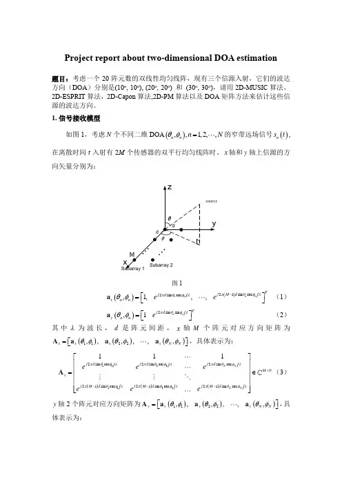
1. 信号接收模型如图1，考虑N 个不同二维DOA (),,1,2,,n n n N θφ=的窄带远场信号()n s t ,在离散时间t 入射有2M 个传感器的双平行均匀线阵时。

x 轴和y 轴上信源的方向矢量分别为：图1()()21sin cos 2sin cos ,1,,,n n n n Tj M d j d x n n e e πθφλπθφθφ-⎡⎤=⎣⎦a （1）()2sin sin ,1n n Tj d y n n e πθφλθφ⎡⎤=⎣⎦a（2）其中λ为波长，d 是阵元间距，x 轴M 个阵元对应方向矩阵为()()()1122,,,,,,x x x x N N θφθφθφ=⎡⎤⎣⎦A a a a ，具体表示为：()()()112211222sin cos 2sin cos 2sin cos 21sin cos 21sin cos 21sin cos 111N NN Nj d j d j d M Nx j M d j M d j M d e e e e e e πθφλπθφλπθφλπθφλπθφλπθφλ⨯---⎡⎤⎢⎥⎢⎥=∈⎢⎥⎢⎥⎢⎥⎣⎦A （3）y 轴2个阵元对应方向矩阵为()()()1122,,,,,,y y y y N N θφθφθφ⎡⎤=⎣⎦A a a a ，具体表示为：112222sin sin 2sin sin 2sin sin 1111N NNy j d j d j d eeeπθφπθφλπθφλ⨯⎡⎤=∈⎢⎥⎣⎦A （4）双平行线阵中子阵列1的接收信号为()()()11x t s t t =+x A n（5）子阵列2的接收信号为()()()22x t t t =+x A Φs n（6）其中()1t n 和()2t n 分别表示子阵列1和2的与信号不相干的加性高斯白噪声，112sin sin 2sin sin ,,N N j d j d diag e e πθφλπθφλ⎡⎤=⎣⎦Φ，()()()11,TN N t s t s t ⨯=∈⎡⎤⎣⎦s 表示信源矢量。

J.Korean Math.Soc.48(2011),No.5,pp.985–999/10.4134/JKMS.2011.48.5.985A FILLED FUNCTION METHOD FOR BOX CONSTRAINEDNONLINEAR INTEGER PROGRAMMINGYoujiang Lin and Yongjian YangAbstract.A newfilled function method is presented in this paper tosolve box-constrained nonlinear integer programming problems.It isshown that for a given non-global local minimizer,a better local min-imizer can be obtained by local search starting from an improved initialpoint which is obtained by locally solving a box-constrained integer pro-gramming problem.Several illustrative numerical examples are reportedto show the efficiency of the present method.1.IntroductionIn[13],Zhu showed that over unbounded domain,the integer programming is undecidable;i.e.,there cannot be any algorithm for the problem.So we consider the following box-constrained discrete global optimization problem: (1.1)min{f(x):x∈X⊂Z n},where f:Z n→R,and Z n is the set of integer points in R n,and X is box;i.e., X={x∈Z n:a≤x≤b,a,b∈Z n}.Like the continuous global optimization problems,the existence of multiple local minima of a general nonconvex objective function makes discrete global optimization a great challenge.For continuous global optimization problems, many deterministic methods(see[1],[7],[8],[10])have been proposed to search for a globally optimal solution of a function of several variables.Thefilled function algorithm(see[2],[4])is an effective and practical method among determinate algorithms.The primaryfilled function was proposed by Ge in paper[2].The definition of thefilled function is as follows:Definition1.1.Assume that x∗1is a current minimizer of f(x).A continuous function P(x)is said to be afilled function of f(x)at x∗1if it satisfies the following properties:Received March8,2010;Revised July26,2010.2010Mathematics Subject Classification.52A10,52A40.Key words and phrases.global optimization,filled function method,nonlinear integer programming,local minimizer,global minimizer.The authors would like to acknowledge the support from the National Natural Science Foundation of China(10971128),Shanghai Leading Academic Discipline Project(S30104).c⃝2011The Korean Mathematical Society985986YOUJIANG LIN AND YONGJIAN YANG(1)x∗1is a maximizer of P(x)and the whole basin B∗1of f(x)at x∗1becomesa part of a hill of P(x);(2)P(x)has no minimizers or saddle points in any higher basin of f(x)than B∗1;(3)If f(x)has a lower basin than B∗1,then there is a point x′in such abasin that minimizes P(x)on the line through x and x∗1.For the definitions of basin and hill,refer to Ge(1990),paper[2].Thefilled function given at x∗1in the paper[2]has the following form:(1.2)P(x,x∗1,r,ρ)=1r+f(x)exp(−∥x−x∗1∥2ρ2),where the parameters r andρneed to be chosen appropriately.The main idea of thefilled function method is to construct an auxiliary func-tion calledfilled function via the current local minimizer of the original opti-mization problem,with the property that the current local minimizer is a local maximizer of the constructedfilled function and a better initial point of the primal optimization problem can be obtained by minimizing the constructed filled function locally.By the same idea as that of solving continuous global optimization problems,We try to solve discrete global optimization problem (1.1).In[3],Ge adapted thefilled function method by Ge[2]for continuous global optimization to the discrete case.However,thefilled function algorithm de-scribed in the paper[2]still has some unexpected features:(i)The efficiency of thefilled function algorithm strongly depend on two parameters r and q.They are not so easy to be adjusted to make them satisfy the needed conditions;(ii)Thefilled function includes exponential terms.If the value of1/ρbe-comes large as iterations proceed,as required to preserve thefilling property, numerical illness may result in failure of computation;(iii)The termination criteria is not good because it requires a large amount of computation before a global minimizer has been found.In this paper,we provide a new definition of the discretefilled function,and a discretefilled function satisfying the definition is presented.An algorithm is developed from the newfilled function.The newfilled function algorithm overcomes the disadvantages mentioned above in a certain extent.Specifically, it has the following several advantages:(i)The newfilled function includes neither exponential terms nor logarithmic terms.Elementary functionϕ(t)=arctan t is used in thefilled function,which possesses many good properties and is efficient in numerical implementations.(ii)The parameters q and r in the newfilled function are easier to be ap-propriately chosen than those of the originalfilled function(1.2).(iii)The new algorithm has a simple termination criteria and the compu-tational results show that this algorithm is more efficient than the original algorithm.A FILLED FUNCTION METHOD987The rest of this paper is organized as follows.In Section2,wefirst re-call some definitions in discrete analysis and discrete optimization.In Section 3,a definition of discretefilled function is given,a discretefilled function is presented,and we investigate its properties.An algorithm is developed and numerical experiments are presented in Section4.Finally,some conclusions are drawn in Section5.2.PreliminaryFirst,we recall some definitions in discrete analysis and discrete optimization (see[11],[12]).Definition2.1.A sequence{x i}u i=−1is called a discrete path in X between two distinct point x∗and x∗∗in X if x−1=x∗,x u=x∗∗,x i∈X for all i; x i=x j for i=j;and∥x0−x∗∥=∥x i+1−x i∥=∥x∗∗−x u−1∥=1for all i.If such a discrete path exists,then x∗and x∗∗are said to be pathwise connected in X.Furthermore,if every two distinct points in X are pathwise connected in X,then X is called a pathwise connected set.Definition2.2.The set of all axial directions in Z n is defined by D={±e i: i=1,2,...,n},where e i is the i th unit vector;The set of all feasible directions at x∈X is defined by D x={d∈D:x+d∈X},where D is the set of axial directions.Definition2.3.For any x∈Z n,the discrete neighborhood of x is defined by N(x)={x,x±e i:i=1,2,...,n};The discrete interior of X is defined by int X={x∈X:N(x)⊆X}.While,the discrete boundary of X is denoted by∂X=X/int X.Definition2.4.A point x∗∈X is called a discrete local minimizer of f over X if f(x∗)≤f(x)for all x∈X∩N(x∗).If,in addition,f(x∗)<f(x)for all x∈X∩N(x∗)/{x∗},then x∗is called a strict discrete local minimizer of over X;A point x∗∈X is called a discrete global minimizer of f over X if f(x∗)≤f(x)for all x∈X.If,in addition,f(x∗)<f(x)for all x∈X,then x∗is called a strict discrete global minimizer of f over X.Definition2.5.For any x∈X,d∈D is said to be a discrete descent direction of f at x over X if x+d∈X and f(x+d)<f(x);beside,d∗∈D is called a discrete steepest descent direction of f at x over X if f(x+d∗)≤f(x+d)for all d∈D∗,where D∗is the set of all descent direction of f at x over X. Algorithm2.6.(Discrete steepest descent method).1.Start from the initial point x∈X.2.If x is a local minimizer of f over X,then stop.Otherwise,a discrete steepest descent direction d∗of f at x over X can be found.3.Let x:=x+λd∗,whereλ∈Z+is the step length such that f has maximum reduction in direction d∗,and go to Step2.988YOUJIANG LIN AND YONGJIAN YANGAlgorithm 2.7.(Modified discrete descent method).1.Start from the initial point x ∈X .2.If x is a local minimizer of f over X ,then stop.Otherwise,letd ∗=argmin {f (x +d i ):d i ∈D x ,f (x +d i )<f (x )},where D x denotes the set of feasible directions at x .3.Let x :=x +d ∗,and go to Step 2.Obviously,by Algorithms 2.6and 2.7,we can only find a discrete local minimizer.Finally,for the discrete global optimization problem (1.1),we make the following assumptions in this paper:Assumption 2.8.X ⊆Z n is a bounded set which contains more than one point.This implies that there exists a constant K >0such that1≤K =max x,y ∈X∥x −y ∥≤∞,where ∥·∥is the usual Euclidean norm.Assumption 2.9.f :∪x ∈X N (x )→R satisfies the following Lipschiz condi-tion for every x,y ∈∪x ∈X N (x ):|f (x )−f (y )|≤L ∥x −y ∥,where 0<L <∞is a constant,N (x )is the discrete neighborhood of x .3.A filled function and its propertiesIn this section,we propose a filled function of f (x )at a current local mini-mizer and discuss its properties.LetS 1={x :|f (x )≥f (x ∗1),x ∈X \{x ∗1}},S 2={x |f (x )<f (x ∗1),x ∈X }.Definition 3.1.P (x,x ∗1)is called a discrete filled function of f (x )at a discrete local minimizer x ∗1if P (x,x ∗1)has the following properties:(1)x ∗1is a strict discrete local maximizer of P (x,x ∗1)on X ;(2)P (x,x ∗1)has no discrete local minimizers in the region S 1;(3)If x ∗1is not a discrete global minimizer of f (x ),then P (x,x ∗1)does havea discrete minimizer in the region S 2.Now,we give a discrete filled function for problem (1.1)at a local minimizer x ∗1as follows:F (x,x ∗1,q,r )=1q +∥x −x ∗1∥ϕq (max {f (x )−f (x ∗1)+r,0}),(3.1)whereϕq (t )={arctan (−qt )+π2,if t =0,0,if t =0.(3.2)r=0.2q>0and r satisfies0<r<maxx∗,x∗1∈L(P)f(x∗)<f(x∗1)(f(x∗1)−f(x∗))where L(P)stand for the set of discrete local minimizers of f(x).A simple example is given in Figure1.Next we will show that the function F(x,x∗1,q,r)is a discretefilled function satisfying Definition3.1under certain conditions on the parameters q and r. Theorem3.2.Suppose that X holds Assumption2.8.Further suppose that x∗1 is a discrete local minimizer of f(x).For any r>0,when q>0is satisfactorily small,x∗1is a strict discrete local maximizer of F(x,x∗1,q,r).Proof.Since x∗1is a discrete local minimizer of f(x)for any x∈N(x∗1)∩X, f(x)≥f(x∗1)and∥x−x∗1∥=1.Hence,we haveF(x,x∗1,q,r)=1q+1(arctan(−qf(x)−f(x∗1)+r)+π2)andF(x∗1,x∗1,q,r)=1q(arctan(−qr)+π2),990YOUJIANG LIN AND YONGJIAN YANGwhen x ≥y ,arctan(x )−arctan(y )≤x −y ;let q <r ,we haveF (x,x ∗1,q,r )−F (x ∗1,x ∗1,q,r )=1q +1(arctan(−q f (x )−f (x ∗1)+r )+π2)−1q (arctan(−q r )+π2)=1q +1arctan(−q f (x )−f (x ∗1)+r )−1q arctan(−q r )+−1q (q +1)π2=1q +1×(arctan(q r )−arctan(q f (x )−f (x ∗1)+r ))+1q ×(q +1)(arctan(q r )−π2)<1q ×(q +1)×(q ×(q r −q f (x )−f (x ∗1)+r )+(arctan 1−π2))=1q ×(q +1)×(q 2×f (x )−f (x ∗1)r ×(f (x )−f (x ∗1)+r )−π4)≤1q ×(q +1)×(q 2×L ∥x −x ∗1∥r 2−π4)=1q ×(q +1)×(q 2×L r 2−π4)≤1q ×(q +1)×(q ×L r −π4).Therefore,when 0<q <min {r,πr 4L },we have F (x,x ∗1,q,r )−F (x ∗1,x ∗1,q,r )<0for any x ∈N (x ∗1)∩X ,x ∗1is a strict discrete local maximizer of F (x,x ∗1,q,r ).□Lemma 3.3.For every x ,x ∗∈X ,if there exits i ∈{1,2,...,n }such that x ±e i ∈X ,then there exists d ∈D such that∥x +d −x ∗∥>∥x −x ∗∥.Proof.If there is an i ∈{1,2,...,n }such that x ±e i ∈X ,then either ∥x +e i −x ∗∥>∥x −x ∗∥or ∥x −e i −x ∗∥>∥x −x ∗∥,therefore we let d =e i or d =−e i ,this completes the proof.□Theorem 3.4.Suppose that Assumptions 2.8-2.9are satisfied.If x ∗1is a discrete local minimizer of f (x ),then the function F (x,x ∗1,q,r )has no discrete local minimizers in the region S 1={x |f (x )≥f (x ∗1),x ∈X/{x ∗1}}when r >0and q >0are satisfactorily small.Proof.Let ˜X =∪x ∈X N (x ),obviously,˜X holds Assumptions 2.8-2.9,and wehave S 1⊆X ⊆int ˜X.For every x ∈S 1,by Lemma 3.3,there must exists a direction d ∈D such that x +d ∈X and∥x +d −x ∗1∥>∥x −x ∗1∥.A FILLED FUNCTION METHOD991 Consider the following two cases:(1)f(x+d)≥f(x∗1):Since f(x+d)≥f(x∗1),we haveF(x+d,x∗1,q,r)−F(x,x∗1,q,r)=1q+∥x+d−x∗1∥(arctan(−qf(x+d)−f(x∗1)+r)+π2)−1q+∥x−x∗1∥(arctan(−qf(x)−f(x∗1)+r)+π2)=1q+∥x+d−x∗1∥arctan(−qf(x+d)−f(x∗1)+r)−1q+∥x−x∗1∥arctan(−qf(x)−f(x∗1)+r)+∥x−x∗1∥−∥x+d−x∗1∥(q+∥x+d−x∗1∥)(q+∥x−x∗1∥)π2=1q+∥x+d−x∗1∥×(arctan(q∗1)−arctan(q∗1))+∥x+d−x∗1∥−∥x−x∗1∥(q+∥x+d−x∗1∥)(q+∥x−x∗1∥)(arctan(qf(x)−f(x∗1)+r)−π2).If f(x)>f(x+d),thenarctan(qf(x)−f(x∗1)+r)−arctan(qf(x+d)−f(x∗1)+r)<0therefore when q<r,we have arctan(qf(x)−f(x∗1)+r)−π2<0,henceF(x+d,x∗1,q,r)−F(x,x∗1,q,r)<0.If f(x)≤f(x+d)for any x,y∈R,when x≤y,we have arctan y−arctan x≤y−x,let q<r and q<1,we haveF(x+d,x∗1,q,r)−F(x,x∗1,q,r)≤1q+∥x+d−x∗1∥×(qf(x)−f(x∗1)+r−qf(x+d)−f(x∗1)+r)+∥x+d−x∗1∥−∥x−x∗1∥(q+∥x+d−x∗1∥)(q+∥x−x∗1∥)(arctan1−π2)≤qq+∥x+d−x∗1∥×(f(x+d)−f(x)(f(x)−f(x∗1)+r)(f(x+d)−f(x∗1)+r))+∥x+d−x∗1∥−∥x−x∗1∥(q+∥x+d−x∗1∥)(2∥x−x∗1∥)(arctan1−π2)≤1(q+∥x+d−x∗1∥)(2∥x−x∗1∥)992YOUJIANG LIN AND YONGJIAN YANG×(2qL∥d∥∥x−x∗1∥r2−π4(∥x+d−x∗1∥−∥x−x∗1∥)).Hence,for any given x∈S1and d,when q is satisfactorily small thatq<πr2(∥x+d−x∗1∥−∥x−x∗1∥)8L∥x−x∗1∥,we haveF(x+d,x∗1,q,r)<F(x,x∗1,q,r).(2)f(x+d)<f(x∗1):In this case,it is clear that f(x+d)<f(x),sincefunction f(t)=arctan(−qt )+π2is increasing about t,hence,we haveF(x+d,x∗1,q,r)<F(x,x∗1,q,r).The above two cases imply that any x∈S1is not the discrete local minimizer of F(x,x∗1,q,r)when q is satisfactorily small.□Theorem3.5.If x∗1is not a discrete global minimizer of f(x)in X,then there exists a discrete minimizer¯x1∗of F(x,x∗1,q,r)in the region S2={x|f(x)< f(x∗1),x∈X}.Proof.Since x∗1is not a discrete global minimizer and F(x,x∗1,q,r)≥0,there exist a point¯x1∗∈S2and r such that f(¯x1∗)<f(x∗1)−r.Hence,F(¯x1∗,x∗1,q,r) =0,it implies that¯x∗1∈S2is a discrete minimizer of F(x,x∗1,q,r).□Theorem3.2,Theorem3.4,and Theorem3.5show that the function F(x, x∗1,q,r)at point x∗1is a discretefilled function satisfying Definition3.1with satisfactorily small q and r.The following theorems further show that the proposedfilled function has some good properties which classical functions have.Theorem3.6.Suppose that Assumption2.9is satisfied.If x1,x2∈X and satisfy the following conditions:(1)f(x1)≥f(x∗1)and f(x2)≥f(x∗1),(2)∥x2−x∗1∥>∥x1−x∗1∥.Then,when r>0and q>0are satisfactorily small,F(x2,x∗1,q,r)<F(x1,x∗1,q,r).Proof.Consider the following two cases:(1)If f(x∗1)≤f(x2)≤f(x1),then it is obvious that the result follows.(2)If f(x∗1)≤f(x1)<f(x2),the result also holds(see the proof process in Theorem3.4).□Theorem3.7.If x1,x2∈X and satisfy the following conditions:(1)∥x2−x∗∥>∥x1−x∗∥,(2)f(x1)≥f(x∗1)>f(x2),and f(x2)−f(x∗1)+r>0.Then,we have F(x2,x∗1,r,q)<F(x1,x∗1,r,q).A FILLED FUNCTION METHOD993 Proof.By Conditions1and2,we have1q+∥x2−x∗1∥<1q+∥x1−x∗1∥and0<f(x2)−f(x∗1)+r<f(x1)−f(x∗1)+r.Hence F(x2,x∗1,r,q)<F(x1,x∗1,r,q).□Now we make some remarks.Firstly,in the phase of minimizing the new discretefilled function,Theorems3.6and3.7guarantee that the current dis-crete local minimizer x∗1of the objective function is escaped and the minimum of the new discretefilled function will be always achieved at a point where the objective function value is less than the current discrete minimum.Secondly, the parameters q and r are easier to be appropriately chosen.In the next section,a new discretefilled function algorithm is given.4.Algorithm and numerical resultsBased on the theoretical results in the previous section,a global optimization algorithm over X is proposed as follows:AlgorithmInitialization:(1)Choose any x0∈X as an initial point.(2)Letε=10−5and q0=0.01.(3)Let D0={±e i:i=1,2,...,n}.Main Program:(1)Starting from initial point x0,minimize f(x)(x∈X)by the discretesteepest descent method(see Algorithm2.1),we can obtain the discretelocal minimizer x∗1.Let r=1,q=q0and D=D0.(2)Construct the discretefilled function:F(x,x∗1,q,r)=1q+∥x−x∗∥ϕq(max{f(x)−f(x∗1)+r,0}),whereϕq(t)={arctan(−qt)+π2,if t=0, 0,if t=0.(3)If r≤ε,then terminate the iteration,the x∗k is the global minimizer off(x),otherwise,the next step.(4)If D=∅,then goto(6),otherwise the next step.(5)If q<ε×10−2,then let r=r/10,q=q0/10and D=D0,goto(2);otherwise let q=q/10,goto(2).(6)Take a direction d∈D,and D←D/{d},turn to Inner Loop.994YOUJIANG LIN AND YONGJIAN YANGInner Loop:(1)k=0.(2)Let y k=x∗1+d.(3)Minimize F(x,x∗1,q,r),starting from the point y k,by implementing themodified discrete descent method(see Algorithm2.2).y k+1denotes thenext iterative point.(4)If y k+1/∈X,then return Main Program(4),otherwise next step.(5)If f(y k+1)≤f(x∗1),then let x0=y m+1and return Main program(1),otherwise let k=k+1and goto Inner Loop(3).In the following part,several test problems are given and results of the algorithm in solving these problems are reported.Through out the tests,we use the modified discrete descent method as shown in Algorithm2.7to perform local searches,in the initialization of the algorithm we let q=0.01and r=1. The algorithm in Fortran95is successfully used tofind the global minimizers of these test problems.The main iterative results are summarized in tables for each function.The symbols used are shown as follows:k:The iteration number infinding the k th local minimizer.x0 k or y0k:The k th initial point.f(x0k )or f(y0k):The function value of the k th initial point.x∗k or y∗k:The k th local minimizer.f(x∗k )or f(y∗k):The function value of the k th local minimizer.Problem4.1.min f(x)=100(x2−x21)2+(1−x1)2+90(x4−x23)2+(1−x3)2,+10.1[(x2−1)2+(x4−1)2]+19.8(x2−1)(x4−1), s.t.10≤x i≤10,i=1,2,3,4.This problem is a discrete counterpart of the problem38in[6].It is a box constrained nonlinear integer programming problem.It has214≈1.94×105 feasible points where41of them are discrete local minimizers but only one of those discrete local minimizers is the discrete global minimum solution:x∗global =(1,1,1,1)with f(x∗global)=0.Let x01=(9,6,5,6)and x01=(9,−9,−9,9),a summary of the computational results are displayed in Tables 1and2.Problem4.2.min f(x)=g(x)h(x),s.t.x i=0.001y i,−2000<y i<2000,i=1,2,where y i(i=1,2)is integer,andg(x)=1+(x1+x2+1)2(19−14x1+3x21−14x2+6x1x2+3x2),h(x)=30+(2x1−3x2)2(18−32x1+12x21+48x2−36x1x2+27x22).A FILLED FUNCTION METHOD995 Table1.Problem4.1initial point is(9,6,5,6)k x0k f(x0k)x∗kf(x∗k)1(9,6,5,6)596070.0(3,8,3,8)2158.0000 2(3,10,2,5)1887.5000(3,8,2,3)1007.5000 3(3,10,1,1)922.1000(3,8,0,−1)453.1000 4(2,5,0,−1)235.6000(2,4,0,0)43.6000 5(1,1,0,0)11.1000(1,1,1,1)0.0000 Table2.Problem4.1initial point is(9,−9,−9,9)k x0k f(x0k)x∗kf(x∗k)1(9,−9,−9,9)1276796.40(3,8,−3,8)2170.0000 2(3,10,−2,5)1895.5000(3,8,−2,3)1015.5000 3(3,10,−1,1)926.1000(3,8,0,−1)453.1000 4(2,5,0,−1)235.6000(2,4,0,0)43.6000 5(1,1,0,0)11.1000(1,1,1,1)0.0000Table3.Problem4.2k y0k f(y0k)y∗kf(y∗k)1(1000,1000)1876.000(1280,890)954.13822(2000,632)951.2482(1609,71)92.34253(1379,2000)19.4895(85,2000)−210795.62531(−1000,−1000)1890.000(0,−1000) 3.0000002(0,1740)−256.5294(85,2000)−210795.62531(2000,2000)35028.000(1280,890)954.13822(2000,632)951.2482(1609,71)92.34263(1379,2000)19.4895(85,2000)−210795.62531(−2000,−2000)20811.9999(0,−1000) 3.0000002(0,1740)−256.5294(85,2000)−210795.6253 This problem is a discrete counterpart of the Goldstein and Price’s function in[5].It is a box constrained nonlinear integer programming problem.It has 40012≈1.60×107feasible points.More precisely,it has207and2discrete local minimizers in the interior and the boundary of box−2.00≤x i≤2.00,i=1,2, respectively.Nevertheless,it has only one discrete global minimum solution:y∗global =(85,2000)with f(y∗global)=−210795.6253.We used four initial pointsin our experiment:(1000,1000),(−1000,−1000),(2000,2000),(−2000,−2000), a summary of the computational results are displayed in Table3.Problem4.3(Beale’s function).min f(x)=[1.5−x1(1−x2)]2+[2.25−x1(1−x22)]2+[2.625−x1(1−x32)]2,996YOUJIANG LIN AND YONGJIAN YANGTable4.Problem4.3k y0k f(y0k)y∗kf(y∗k)1(3000,5000)146039.2031(−3,9735) 6.06732(10000,963) 6.0183(3015,504)3.7589×10−5 1(−3000,−5000)150120.7031(11,−5964)9.02302(10000,788)8.9179(3015,504)3.7589×10−5 1(8000,8000)16992808.2031(−3,9735) 6.06732(10000,963) 6.0183(3015,504)3.7589×10−5 1(−8000,−8000)17121524.2031(5,−7842)8.67812(10000,790)8.6132(3015,504)3.7589×10−5Table5.Problem4.4k y0k f(y0k)y∗kf(y∗k)1(−5000,−5000,−5000,−5000)3650.0000(−116,12,55,−56)3.7213×10−4 2(−78,8,38,−38)7.9387×10−5(−79,8,38,−38)7.9045×10−5 3(11,−1,11,11)1.2798×10−6(10,−1,11,11)2.7985×10−7 4(0,0,3,3)2.1060×10−9(0,0,1,1)2.6000×10−11 1(5000,5000,5000,5000)3650.0000(116,−12,56,57)3.7859×10−4 2(78,−8,38,38)7.9387×10−5(79,−8,38,38)7.9045×10−5 3(−11,1,−11,−11)1.2798×10−6(−10,1,11,−11)2.7985×10−7 4(0,0,3,−3)2.1060×10−9(0,0,1,−1)2.6000×10−11Table6P N DN IN T I F N1450.236049532230.070732317673220.05216224364444278.245675801758525247.49104950368555021147.47298451600510024406.341276667658625242.6725336724326502249.264535436658610023087.764275437056s.t.x i=0.001y i,−104≤y i≤104,i=1,2,where y i(i=1,2)is integer.This problem is discrete counterpart if the problem203in[9].It is a box constrained nonlinear integer programming problem.It has200012≈4.00×108 feasible points and many discrete local minimizers,but it has only one discreteA FILLED FUNCTION METHOD 997Table parison of the resultsGe’s algorithm New algorithm PN DN IN TI F N RA IN TI F N RA 1.41073.667707461.22−4638.564466530.47−5321837.5366175644.73−311328.102295761.78−512657.0751126852.03−38375.807522360.38−435866.2673855076.12−418406.542453513.80−618659.5161008410.24−415315.345500551.67−62.21157.36723520.10−4648.0512303.15−613168.74265900.67−56123.0985675.03−71389.52763501.25−4631.9165850.72−63.263454.3553674598.07−412982.440134223.90−567098.6216532109.12−4101752.812179839.92−64.42012873.31053243183.19−3162577.1205453901.10−5205952.54630876415.00−416214.3423166343.00−65.253228750.21783421091.05−6181524.7083452972.13−7326532.0972*******.09−618352.761965312.20−7316098.73230678124.56−619213.450882064.12−76.25181105.5503680560.06−525428.650309874.31−818963.2712987675.01−525320.710756183.00−8182544.3268021142.10−523484.56289457.00−7183245.71123547700.38−525145.3542345528.29−8global minimum solution y ∗global =(3000,500)with f (y ∗global )=0.We used four initial points in our experiment:(3000,5000),(−3000,−5000),(8000,8000),(−8000,−8000),a summary of the computational results are displayed in Table 4.Problem 4.4(Powell’s singular function).min f (x )=(x 1+10x 2)2+5(x 3−x 4)2+(x 2−2x 3)4+10(x 1−x 4)4,s .t .x i =0.001y i ,−104≤y i ≤104,i =1,2,3,4,where y i (i =1,2,3,4)is integer.It is a box constrained nonlinear integer programming problem.It has 200014≈1.60×1017feasible points and many local minimizers,but it hasonly one global minimum solution:y ∗global =(0,0,0,0)with f (y ∗global )=0.We used two initial points in our experiment:(−5000,−5000,−5000,−5000),(5000,5000,5000,5000),a summary of the computational results are displayed in Table 5.Problem 4.5.min f (x )=(x 1−1)2+5(x n −1)2+n −1∑i =1(n −i )(x 2i −x i +1)2,s .t .−5≤y i ≤5,i =1,2,...,n.998YOUJIANG LIN AND YONGJIAN YANGThis problem is a generalization of the problem282in[9].It is a box con-strained nonlinear integer programming problem.It has11n feasible points andmany local minimizers,but it has only one global minimum solution:x∗global =(1,...,1)with f(x∗global )=0.For all problem with different size,we used fourinitial points in our experiment:(5,...,5),(−5,...,−5),(−5,...,−5,5,...,5), (5,...,5,−5,...,−5).For every experiment,the proposed algorithm succeeded in identifying the discrete global minimum.Let x01=(5,...,5),for n= 25,50,100,respectively,the summary of the computational results are dis-played in Table6.Problem4.6(Rosenbrock’s function).min f(x)=n−1∑i=1[100(x i+1−x2i)2+(1−x i)2],s.t.−5≤y i≤5,i=1,2,...,n.It is a box constrained/unconstrained nonlinear integer programming prob-lem.It has11n feasible points and many local minimizers,but it has onlyone global minimum solution:x∗global =(1,1,...,1)with f(x∗global)=0.Forall problems with different sizes,we used four initial points in our experiment: (5,...,5),(−5,...,−5),(−5,...,−5,5,...,5),(5,...,5,−5,...,−5).For ev-ery experiment,the proposed algorithm succeeded in identifying the discrete global minimum.Let x01=(5,...,5),for n=25,50,100,respectively,the summary of the computational results are displayed in Table6.In Table6,we give the experiment results for Problems4.1-4.6.In Table7, Problems4.1-4.6.with2to25variables are tested and the table shows that in most cases the newfilled function algorithm works better than Ge’sfilled function algorithm.The symbols used in Tables6-7are shown as follows: P N:The N th problem.DN:The dimension of objective function of a problem.IN:The number of iteration cycles.T I:The CPU time in seconds for the algorithm to stop.F N:The number of objective function evaluations for algorithm to stop.RA:The ratio of the number of function evaluations to the number of feasible points.5.ConclusionsThis paper gives a definition of thefilled function for the nonlinear integer programming problem,and presents a newfilled function.Afilled function algorithm based on this givenfilled function is designed.The implementation of the algorithm on several test problems is reported with satisfactory numerical results.A FILLED FUNCTION METHOD999 Acknowledgment.The authors are most grateful to the referee for his many excellent suggestions for improving the original manuscript.References[1] B.C.Cetin,J.Barhen,and J.W.Burdick,Terminal repeller unconstrained subenergytunneling(TRUST)for fast global optimization,J.Optim.Theory Appl.77(1993),no.1,97–126.[2]R.P.Ge,Afilled function method forfinding a global minimizer of a function of severalvariables,Math.Programming46(1990),no.2,(Ser.A),191–204.[3]R.P.Ge and C.B.Huang,A continuous approach to nonlinear integer programming,put.34(1989),no.1,part I,39–60.[4]R.P.Ge and Y.F.Qin,The globally convexizedfilled functions for global optimization,put.35(1990),no.2,part II,131–158.[5] A.A.Goldstein and J.F.Price,On descent from local minima,p.25(1971),569–574.[6]W.Hock and K.Schittkowski,Test Examples for Nonlinear Programming Codes,Springer,NewYork,1981.[7]R.Horst,P.M.Pardalos,and N.V.Thoai,Introduction to Global Optimization,seconded.,Kluwer Academic Publishers,Dordrecht,2000.[8] A.V.Levy and A.Montalvo,The tunneling algorithm for the global minimization offunctions,SIAM put.6(1985),no.1,15–29.[9]K.Schittkowski,More Test Examples for Nonlinear Programming Codes,Springer,NewYork,1987.[10]Y.Yao,Dynamic tunneling algorithm for global optimization,IEEE Trans.SystemsMan Cybernet.19(1989),no.5,1222–1230.[11]L.S.Zhang,F.Gao,and W.X.Zhu,Nonlinear integer programming and global opti-mization,put.Math.17(1999),no.2,179–190.[12]W.X.Zhu,An approximate algorithm for nonlinear integer programming,Appl.Math.Comput.93(1998),no.2-3,183–193.[13],Unsolvability of some optimization problems,put.174(2006),no.2,921–926.Youjiang LinDepartment of MathematicsShanghai UniversityShanghai200444,P.R.ChinaE-mail address:linyoujiang@Yongjian YangDepartment of MathematicsShanghai UniversityShanghai200444,P.R.ChinaE-mail address:yjyang@。

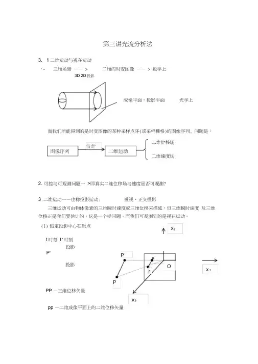
第三讲光流分析法3. 1二维运动与视在运动1- 三维场景 —— >二维的时变图像 —— > 数学上3D 2D 投影而我们所能得到的是时变图像的某种采样点阵(或采样栅格)的图像序列, 问题是：2. 可控与可观测问题一 >即真实二维位移场与速度是否可观测? 三维运动可由物体像素的三维瞬时速度或三维位移来描述，但三维瞬时速度 及三维位移正是我们要估计的，这是一个逆问题。

而我们可观测到的是视在运动。

(1) 假定投影中心在原点t '时刻投影pp —二维成像平面上的二维位移矢量成像平面，投影平面 光学上3.二维运动——也称投影运动:透视、正交投影t 时刻 P '投影PP —三维位移矢量二维位移场 二维速度场(2) 假定投影中心在O i 点 由于投影作用，从P 点出发，终点在O i P /虚线上的三维位移矢 量均有相同的二维投影位移矢量。

所以说，投影的结果只是三维真实 运动的部分信息。

(3) 设(X,t) R 3, t t l t 由像素的运动S c(X ，t) d c(X,t,t ')对应于点阵A 3 ，则有d p (X,t ; l t) d c (X,t ; l t)，假定三维瞬时速度为(X i ,X 2,X 3)，则V p (X,t) V c ( n,k)4. 光流场与对应场(1) pp 定义为对应矢量光流矢量定义为某点(X,t) R 3上的图像平面坐标的瞬时变化率， 为一个导数。

V (V i ,V 2 )T (dx i /dt,dx 2/dt)T表征了时空变化，而且是连续的变化。

(2) 当t t t 0时，则光流矢量与对应矢量等价。

如果在某个点阵A 3可 观测到这种变化，则就意义对应场 <——像素的二维位移矢量场 光流场 <――像素的二维速度矢量场 也分别称为二维视在对应场与速度场。

一般而言，对应矢量 工位移场光流矢量工速度场二维位移矢量函数(x ，t ) A 3d (n,k ； I) d p (X,t ; l t)(n ，k )Z 3k 表达了 t ‘- t 的时间离散n (n i , n 2)T光照变化—— ＞将防碍二维运动场的估计。

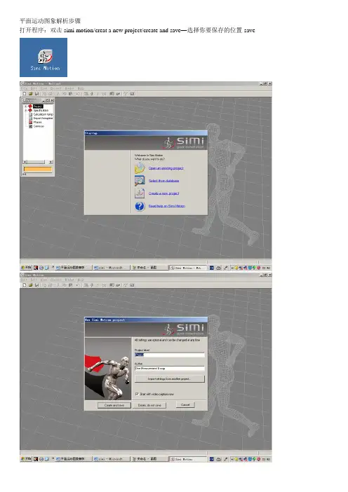
平面运动图象解析步骤打开程序：双击simi motion/creat a new project/create and save—选择你要保存的位置-save平面图像解析的步骤：一、建模（creating a sepcification）二、坐标换算（calibrating the camera）三、打点（获取象坐标,capturing the image coordinates）四、数值计算（calculating the scaled 2-D coordinates）五、数据输出（presenting the data）一、建模（creating a sepcification）建模的目的就是把人体简化为多刚体模型，通过选择相应的关节点并对关节点进行连线，从而形成人体棍图模型。

建模块包括2项内容：A．编辑坐标点(edit points)；B．连接坐标点(connections)A．编辑坐标点：操作：Specification-points-(左键按住拖拽至右边黑色区域，或者在上单击右键-edit)a.把左侧的predefined栏中已设置的点拖拽到右边的uesed points栏中b.对选择后的坐标点的名称和颜色进行编辑：在所选坐标点上右击-property,进行编辑c.编辑软件中未设置的关节点：在uesed points栏里的空隙处点击右键，选择add添加新的关节点，并编辑坐标点B．连接坐标点：两个坐标点连接就会形成一个人体的环节，程序有默认的常规的环节的连线，如大腿是髋关节点与膝关节点的连线。

出于分析的需要，需要在某些关节点之间建立连线，此时需要我们添加新的连接，方法如下：操作：将左键按住拖拽到右边的灰色区域（或者在其上右击后选择edit）New connections—编辑连接名(例如头-脚跟)—选择起始点（starting point）--line to –结束点/apply如果需要在单个点的周围划圈，则只需要选circle with radius，确定圆圈大小即可。