The Euclidean Space

欧式空间练习题欧式空间（Euclidean space）是指以欧几里德几何学为基础的一种空间，其中包含了平面和三维空间。

在欧式空间中，我们可以进行各种几何运算和推理，探索数学中的各种定理和性质。

为了加深对欧式空间的理解和应用，以下将给出一些欧式空间的练习题，并解答相关问题。

题目一：平面上两点坐标求距离已知平面上两点坐标分别为A（2，3）和B（-1，5），求AB两点之间的距离。

解答一：根据两点之间的距离公式，我们可以得出AB两点之间的距离为：d = √((x₂-x₁)² + (y₂-y₁)²)其中，(x₁, y₁)表示A点坐标，(x₂, y₂)表示B点坐标。

代入A（2，3）和B（-1，5）的坐标，计算得：d = √((-1-2)² + (5-3)²)= √((-3)² + 2²)= √(9 + 4)= √13所以，AB两点之间的距离为√13。

题目二：三维空间两点坐标求距离已知三维空间中，点A坐标为（1，2，3），点B坐标为（4，5，6），求AB两点之间的距离。

解答二：同样利用两点之间的距离公式，在三维空间中计算AB两点之间的距离：d = √((x₂-x₁)² + (y₂-y₁)² + (z₂-z₁)²)代入A（1，2，3）和B（4，5，6）的坐标，得：d = √((4-1)² + (5-2)² + (6-3)²)= √(3² + 3² + 3²)= √(9 + 9 + 9)= √27= 3√3所以，AB两点之间的距离为3√3。

题目三：欧式空间的垂直关系判断已知平面上的三个点A（1，2），B（-2，4），C（3，6），判断AB和AC两条线段是否垂直。

解答三：两条线段AB和AC垂直的条件是它们的斜率互为负倒数，即斜率乘积为-1。

我们可以分别计算AB和AC的斜率，然后判断其乘积是否为-1。

一百年前的数学界有两位泰斗：庞加莱和希尔伯特，而尤以后者更加出名，我想主要原因是他曾经在1900年的世界数学家大会上提出了二十三个著名的希尔伯特问题，指引了本世纪前五十年数学的主攻方向，不过还有一个原因呢，我想就是著名的希尔伯特空间了。

希尔伯特空间是希尔伯特在解决无穷维线性方程组时提出的概念，原来的线性代数理论都是基于有限维欧几里得空间的，无法适用，这迫使希尔伯特去思考无穷维欧几里得空间，也就是无穷序列空间的性质。

大家知道，在一个欧几里得空间R^n上，所有的点可以写成为：X=（x1，x2，x3，...，xn）。

那么类似的，在一个无穷维欧几里得空间上点就是：X= （x1，x2，x3，....xn，.....），一个点的序列。

欧氏空间上有两个重要的性质，一是每个点都有一个范数（绝对值，或者说是一个点到原点的距离），||X||^2=∑xn^2，可是这一重要性质在无穷维时被破坏了：对于无穷多个xn，∑xn^2可以不存在（为无穷大）。

于是希尔伯特将所有∑xn^2为有限的点做成一个子空间，并赋以X*X'=∑xn*xn' 作为两点的内积。

这个空间我们现在叫做l^2，平方和数列空间，这是最早的希尔伯特空间了。

注意到我只提了内积没有提范数，这是因为范数可以由点与自身的内积推出，所以内积是一个更加强的条件，有内积必有范数，反之不然。

只有范数的空间叫做Banach空间，（以后有时间再慢慢讲:-）。

如果光是用来解决无穷维线性方程组的话，泛函就不会被称为现代数学的支柱了。

Hilbert空间中我只提到了一个很自然的泛函空间：在无穷维欧氏空间上∑xn^2为有限的点。

这个最早的Hilbert space叫做l^2（小写的l 上标2，又叫小l2空间），非常类似于有限维的欧氏空间。

数学的发展可以说是一部抽象史。

最早的抽象大概是一个苹果和一头牛在算术运算中可以都被抽象为“一”，也就是“数学”本身的起源（脱离具体物体的数字运算）了，而Hilbert space理论发展就正是如此：“内积+ 线性”这两个性质被抽象出来，这样一大类函数空间就也成为了Hilbert space。

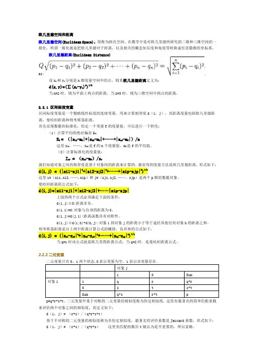
欧几里德空间和距离欧几里德空间(Euclidean Space)，简称为欧氏空间，在数学中是对欧几里德所研究的二维和三维空间的一般化。

所谓一般化就是把欧几里德对于距离、以及相关的概念如长度和角度等转换成任意数维的坐标系。

欧几里德距离(Euclidean Distance)The Euclidean distance between points andin Euclidean n-space, is definedas:.设x n和y n分别是n维度量空间中的点，则其欧几里德距离定义为：d(x,y)=(∑(x i-y i)2)1/2当n=2时，则为平面上两点的距离，当n=3时，则为三维空间中两点的距离。

2.2.1 区间标度变量区间标度变量是一个粗略线性标度的连续变量。

用来计算相异度d（i，j），其距离度量包括欧几里德距离，曼哈坦距离和明考斯基距离。

首先实现数据的标准化，给定一个变量f的度量值，可以进行一下转化：（1）计算平均的绝对偏差S f：S f = （|x1f-m f|+|x2f-m f|+……+|x nf-m f|）/n这里x1f，……，x nf是f的n个度量值，m f是f的平均值。

（2）计算标准化的度量值：Z if = （x if-m f）/s f我们知道对象之间的相异度是基于对象间的距离来计算的。

最常用的度量方法是欧几里德距离，形式如下：d(i,j) = (|xi1-xj1|2+|xi2-xj2|2+……+|xip-xjp|2)1/2这里i=（xi1,xi2,……,xip）和j=（xj1,xj2,……，xjp）是两个p维的数据对象。

曼哈坦距离的公式如下：d(i,j)=|xi1-xj1|+|xi2-xj2|+……|xip-xjp|上面的两个公式必须满足下面的条件：d(i,j)≧0:距离非负。

d(i,i)=0:对象与自身的距离为0。

d(i,j)=d(j,i):距离函数具有对称性。

d(i,j)≦d(i,h)+d(h,j):对象i到对象j的距离小于等于途经其他任何对象h的距离之和。

《线性代数》英文专业词汇序号英文中文1Linear Algebra线性代2determinant行列3row 4column5element元6diagonal对角7principal diagona主对角8auxiliary diagonal次对角9 transposed determinant转置行列10triangular determinants三角行列11the number of inversions逆序12even permutation奇排13odd permutation偶排14parity奇偶15interchange互16absolute value绝对17identity恒等18n-order determinants n 阶行列式19evaluation of determinant行列式的求20 Laplace 's expansion theorem拉普拉斯展开21 cofactor余子22Algebra cofactor代数余子式23the Vandermonde determinant范德蒙行列24 bordered determinant加边行列25reduction of the order of a determinant降阶26method of Recursion relation递推27induction归纳28 Cramer′s rule克莱姆法29matrix矩30 rectangular矩形31the zero matrix零矩阵32the identity matrix单位矩33symmetric对称的序号英文中文34skew-symmetric反对称35commutative law交换36square Matrix方37a matrix of order m ×n矩阵m×n38the determinant of matrix A方阵A 的行39 operations on Matrices矩阵的运40a transposed matrix转置矩41an inverse matrix逆矩42an conjugate matrix共轭矩43an diagonal matrix对角矩44an adjoint matrix伴随矩45singular matrix奇异矩46nonsingular matrix非奇异矩47 elementary transformations初等变48vectors向49components分50linearly combination线性组51space of arithmetical vectors向量空52subspace 子空53dimension54basis55canonical basis规范56coordinates坐57decomposition分58 transformation matrix过渡矩59linearly independent线性无60linearly dependent线性相61the minor of the kth order k 阶子62rank of a Matrix矩阵的63row vectors行向量64column vectors列向量65the maximal linearly independent subsystem最大线性无66Euclidean space欧几里德67Unitary space酉空间序号英文中文68systems of linear equations线性方程69 elimination method消元70homogenous齐次71 nonhomogenous非齐次72equivalent等价73 component-wise分74necessary and sufficient condition充要条75incompatiable无解76unique solution唯一77the matrix of the coefficients系数矩78augmented matrix增广矩79general solution通80particular solution特81trivial solution零82nontrivial solution非零83the fundamental system of solutions基础解84 eigenvalue特征85eigenvector特征向86 characteristic polynomial特征多项87 characteristic equation特征方88scalar product内89normed vector单位向90orthogonal正交91orthogonalization正交92the Gram-Schmidt process正交化过93reducing a matrix to the diagonal form对角化矩94orthonormal basis标准正交95orthogonal transformation正交变换96linear transformation线性97quadratic forms二98canonical form标准型99the canonical form of a quadratic form二次型的标100the method of separating perfect squares 配完全平101the second-order curve二次102 coordinate transformation坐标变换。

《盗梦空间》——数学迷阵导图《盗梦空间》2010 年在全球热映，除了扣人心弦的故事情节外，影片中充满众多数学元素，公理体系、不可能图形、分形几何等等，数不胜数。

本文将剖析其包含的数学文化及其教学意义。

不过，虽然科布的特殊技能，令他在这个贪婪的世界中成为了一个成功的商业间谍，但他为此也付出了沉重的代价。

科布成为企业间谍中令人垂涎的对象，也让他失去了所爱的人，并成为一名国际逃犯。

如今, 柯布接受了一项新任务, 这是他一次救赎的机会, 但是他要做的是潜意识犯罪中最不可能的境界：植入意念，要让一个大企业的继承人自愿解散公司。

如果他们能够成功, 这将会是一次史无前例的完美犯罪。

但无论“盗梦小组”如何精心策划, 这次任务过程中一直有一个神秘敌人如影随形, 而这个神秘人只有柯布能够感应到其存在。

因为犯罪现场存在于人的思想中，他找到了自己的伙伴，要制造出几乎不可能制造出的3 层梦境，在不断躲避潜意识里的守护者的攻击中，他们有一些人进入了潜意识的边缘，看到了他潜意识里的妻子和孩子，他将会怎么选择? 会留在那里和妻子在一起，还是会回到现实? 无论答案是什么都让人揪心撕肺。

《盗梦空间》简介>>> 《盗梦空间》又名《奠基》(Inception)，是由克里斯托弗. 诺兰编剧与导演的，诺兰继《蝙蝠侠前传2: 黑暗骑士》后再次给我们带来了惊喜，剧情扑朔迷离，悬案迭起，使观众游走于梦境与现实之间。

多姆. 科布是一个经验老道的窃贼，在人们精神最为脆弱的时候，他潜入别人梦中，窃取潜意识中有价值的信息和秘密。

在他看来，人类思维所能产生的能量是不可限量的——人们靠思维就可以建造城市，可以穿越时空，回到过去重新制定社会的法则。

人们甚至可以通过思维来进行犯罪。

只可惜，面对如此宝贵的财富，大多数人不知道如何获取。

而科布却恰巧拥有这样奇特的技能。

他利用人们做梦的时候，从他们的潜意识里盗取秘密；因为往往人们在做梦的时候，精神防线是最脆弱的。

n维空间开集的表示摘要：1.引言2.n 维空间开集的定义3.n 维空间开集的表示方法3.1 欧几里得空间中的开集表示3.2 拓扑空间中的开集表示4.结论正文：【引言】在数学中，特别是在拓扑学和相关领域，开集是一个非常重要的概念。

研究不同维度空间中开集的表示方法，有助于我们更好地理解空间结构和性质。

本文将介绍n 维空间开集的表示方法。

【n 维空间开集的定义】在n 维欧几里得空间Euclidean space 中，开集是指一个包含在其内部的点集，这些点集的任意开球（即以任意点为球心，以任意半径为半径的球）都包含在开集中。

在拓扑空间中，开集的定义类似，但要求更宽松，即包含在其内部的任意开集都开。

【n 维空间开集的表示方法】【3.1 欧几里得空间中的开集表示】在欧几里得空间中，开集可以用以下方式表示：1.列出开集中的点的坐标。

2.给定一个点，判断其是否在开集中，只需判断其到开集中任意一点的距离是否小于等于某个正数。

【3.2 拓扑空间中的开集表示】在拓扑空间中，开集的表示较为复杂，需要引入更丰富的概念。

拓扑空间中的开集表示方法如下：1.给定一个开集，找到一个开球，使得该开球包含在开集中。

2.确定开球的半径，即找到一个正数r，使得以开球中心为球心，r 为半径的球包含在开集中。

3.以开球中心为顶点，以r 为半径构建一个开邻域。

4.判断一个点是否在开集中，只需判断该点是否在开邻域内。

【结论】总的来说，n 维空间开集的表示方法依赖于空间的性质和维度。

在欧几里得空间中，我们可以通过列出点的坐标和判断距离来表示开集；而在拓扑空间中，我们需要引入开球和开邻域等概念来表示开集。

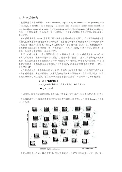
1.什么是流形根据维基百科上的解释： In mathematics, (specially in differential geometry and topology), a manifold is a topological space that in a small enough scale resembles the Euclidean space of a specific dimension, called the dimension of the manifold.因此，一个直线或者一个曲线是一个一维流形，一个平面或者球面是二维流形，依次类推到高维空间。

有时候经常会在 paper 里看到“嵌入在高维空间中的低维流形”，不过高维的数据对于我们这些低维生物来说总是很难以想象，所以最直观的例子通常都会是嵌入在三维空间中的二维或者一维流行。

比如说一块布，可以把它看成一个二维平面，这是一个二维的欧氏空间，现在我们（在三维）中把它扭一扭，它就变成了一个流形（当然，不扭的时候，它也是一个流形，欧氏空间是流形的一种特殊情况）。

所以，直观上来讲，一个流形好比是一个 d 维的空间，在一个 m 维的空间中 (m > d) 被扭曲之后的结果。

流形并不是一个“形状”，而是一个“空间”。

当然，这些都是直观上的概念，其实流形并不需要依靠嵌入在一个“外围空间”而存在，稍微正式一点来说，一个 d 维的流形就是一个在任意点出局部同胚于（简单地说，就是正逆映射都是光滑的一一映射）欧氏空间除了简单的例子，在实际的应用中的数据，我们怎么知道它是不是一个流形呢于是不妨又回归直观的感觉。

再从球面说起，如果我们事先不知道球面的存在，那么球面上的点，其实就是三维欧式空间上的点，可以用一个三元组来表示其坐标。

可以看一下它的参数方程：0 0 0sin cos sin sin cosx x r y y r z z r θϕθϕθ=+=+ =+（02ϕπ≤≤，0θπ≤≤）可以看到，这些三维的坐标实际上是由两个变量θ和ϕ生成的，因此自由度是二，对应了一个二维的流行。

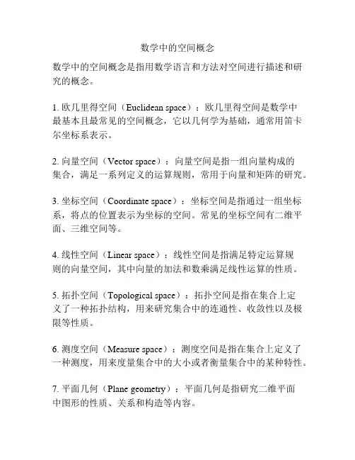
数学中的空间概念
数学中的空间概念是指用数学语言和方法对空间进行描述和研究的概念。

1. 欧几里得空间（Euclidean space）：欧几里得空间是数学中
最基本且最常见的空间概念，它以几何学为基础，通常用笛卡尔坐标系表示。

2. 向量空间（Vector space）：向量空间是指一组向量构成的
集合，满足一系列定义的运算规则，常用于向量和矩阵的研究。

3. 坐标空间（Coordinate space）：坐标空间是指通过一组坐标系，将点的位置表示为坐标的空间。

常见的坐标空间有二维平面、三维空间等。

4. 线性空间（Linear space）：线性空间是指满足特定运算规
则的向量空间，其中向量的加法和数乘满足线性运算的性质。

5. 拓扑空间（Topological space）：拓扑空间是指在集合上定
义了一种拓扑结构，用来研究集合中的连通性、收敛性以及极限等性质。

6. 测度空间（Measure space）：测度空间是指在集合上定义了一种测度，用来度量集合中的大小或者衡量集合中的某种特性。

7. 平面几何（Plane geometry）：平面几何是指研究二维平面
中图形的性质、关系和构造等内容。

8. 立体几何（Solid geometry）：立体几何是指研究三维空间
中立体图形的性质、关系和构造等内容。

9. 代数拓扑（Algebraic topology）：代数拓扑是将代数学方法
应用于拓扑空间研究的一个分支，研究空间的代数性质和变形等问题。

10. 同调论（Homology theory）：同调论是数学中的一个分支，研究空间中的“洞”和“环”等代数特征，用于研究空间的性质和
分类。

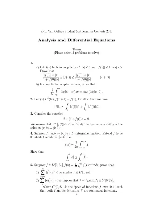
S.-T.Yau College Student Mathematics Contests 2010Analysis and Differential EquationsTeam(Please select 5problems to solve)1.a)Let f (z )be holomorphic in D :|z |<1and |f (z )|≤1(z ∈D ).Prove that|f (0)|−|z |1+|f (0)||z |≤|f (z )|≤|f (0)|+|z |1−|f (0)||z |.(z ∈D )b)For any finite complex value a ,prove that 12π 2π0log |a −e iθ|dθ=max {log |a |,0}.2.Let f ∈C 1(R ),f (x +1)=f (x ),for all x ,then we have ||f ||∞≤ 10|f (t )|dt + 10|f (t )|dt.3.Consider the equation¨x +(1+f (t ))x =0.We assume that ∞|f (t )|dt <∞.Study the Lyapunov stability of the solution (x,˙x )=(0,0).4.Suppose f :[a,b ]→R be a L 1-integrable function.Extend f to be 0outside the interval [a,b ].Letφ(x )=12h x +h x −hf Show thatb a |φ|≤ b a |f |.5.Suppose f ∈L 1[0,2π],ˆf (n )=12π 2π0f (x )e −inx dx ,prove that 1)∞ |n |=0|ˆf(n )|2<∞implies f ∈L 2[0,2π],2)n |n ˆf (n )|<∞implies that f =f 0,a.e.,f 0∈C 1[0,2π],where C 1[0,2π]is the space of functions f over [0,1]such that both f and its derivative f are continuous functions.126.SupposeΩ⊂R3to be a simply connected domain andΩ1⊂Ωwith boundaryΓ.Let u be a harmonic function inΩand M0=(x0,y0,z0)∈Ω1.Calculate the integral:II=−Γu∂∂n(1r)−1r∂u∂ndS,where 1r=1(x−x0)2+(y−x0)2+(z−x0)2and∂∂ndenotes theout normal derivative with respect to boundaryΓof the domainΩ1.(Hint:use the formula∂v∂n dS=∂v∂xdy∧dz+∂v∂ydz∧dx+∂v∂zdx∧dy.)S.-T.Yau College Student Mathematics Contests 2010Applied Math.,Computational Math.,Probability and StatisticsTeam(Please select 5problems to solve)1.Let X 1,···,X n be independent and identically distributed random variables with continuous distribution functions F (x 1),···,F (x n ),re-spectively.Let Y 1<···<Y n be the order statistics of X 1,···,X n .Prove that Z j =F (Y j )has the beta (j,n −j +1)distribution (j =1,···,n ).2.Let X 1,···,X n be i.i.d.random variable with a continuous density f at point 0.LetY n,i =34b n (1−X 2i /b 2n )I (|X i |≤b n ).Show that n i =1(Y n,i −EY n,i )(b n n i =1Y n,i )1/2L −→N (0,3/5),provided b n →0and nb n →∞.3.Let X 1,···,X n be independently and indentically distributed ran-dom variables with X i ∼N (θ,1).Suppose that it is known that |θ|≤τ,where τis given.Showmin a 1,···,a n +1sup |θ|≤τE (n i =1a i X i +a n +1−θ)2=τ2n −1τ2+n −1.Hint:Carefully use the sufficiency principle.4.The rules for “1and 1”foul shooting in basketball are as follows.The shooter gets to try to make a basket from the foul line.If he succeeds,he gets another try.More precisely,he make 0baskets by missing the first time,1basket by making the first shot and xsmissing the second one,or 2baskets by making both shots.Let n be a fixed integer,and suppose a player gets n tries at “1and 1”shooting.Let N 0,N 1,and N 2be the random variables recording the number of times he makes 0,1,or 2baskets,respectively.Note that N 0+N 1+N 2=n .Suppose that shots are independent Bernoulli trails with probability p for making a basket.(a)Write down the likelihood for (N 0,N 1,N 2).12(b)Show that the maximum likelihood estimator of p is ˆp =N 1+2N 2N 0+2N 1+2N 2.(c)Is ˆp an unbiased estimator for p ?Prove or disprove.(Hint:E ˆp is a polynomial in p ,whose order is higher than 1for p ∈(0,1).)(d)Find the asymptotic distribution of ˆp as n tends to ∞.5.When considering finite difference schemes approximating partial differential equations (PDEs),for example,the scheme(1)u n +1j =u n j −λ(u n j −u n j −1)where λ=∆t ∆x ,approximating the PDE (2)u t +u x =0,we are often interested in stability,namely(3)||u n ||≤C ||u 0||,n ∆t ≤T for a constant C =C (T )independent of the time step ∆t and the spa-tial mesh size ∆x .Here ||·||is a given norm,for example the L 2norm orthe L ∞norm,of the numerical solution vector u n =(u n 1,u n 2,···,u n N ).The mesh points are x j =j ∆x ,t n =n ∆t ,and the numerical solutionu n j approximates the exact solution u (x j ,t n )of the PDE (2)with aperiodic boundary condition.(i)Prove that the scheme (1)is stable in the sense of (3)for boththe L 2norm and the L ∞norm under the time step restriction λ≤1.(ii)Since the numerical solution u n is in a finite dimensional space,Student A argues that the stability (3),once proved for a spe-cific norm ||·||a ,would also automatically hold for any other norm ||·||b .His argument is based on the equivalency of all norms in a finite dimensional space,namely for any two norms ||·||a and ||·||b on a finite dimensional space W ,there exists a constant δ>0such thatδ||u ||b ≤||u ||a ≤1δ||u ||b .Do you agree with his argument?If yes,please give a detailed proof of the following theorem:If a scheme is stable,namely (3)holds for one particular norm (e.g.the L 2norm),then it is also stable for any other norm.If not,please explain the mistake made by Student A.6.We have the following 3PDEs(4)u t +Au x =0,(5)u t +Bu x =0,3 (6)u t+Cu x=0,C=A+B.Here u is a vector of size m and A and B are m×m real matrices. We assume m≥2and both A and B are diagonalizable with only real eigenvalues.We also assume periodic initial condition for these PDEs.(i)Prove that(4)and(5)are both well-posed in the L2-norm.Recall that a PDE is well-posed if its solution satisfies||u(·,t)||≤C(T)||u(·,0)||,0≤t≤Tfor a constant C(T)which depends only on T.(ii)Is(6)guaranteed to be well-posed as well?If yes,give a proof;if not,give a counter example.(iii)Suppose we have afinite difference schemeu n+1=A h u nfor approximating(4)and another schemeu n+1=B h u nfor approximating(5).Suppose both schemes are stable in theL2-norm,namely(3)holds for both schemes.If we now formthe splitting schemeu n+1=B h A h u nwhich is a consistent scheme for solving(6),is this scheme guar-anteed to be L2stable as well?If yes,give a proof;if not,givea counter example.S.-T.Yau College Student Mathematics Contests2010Geometry and TopologyTeam(Please select5problems to solve)1.Let S n⊂R n+1be the unit sphere,and R n⊂R n+1the equator n-plane through the center of S n.Let N be the north pole of S n.Define a mappingπ:S n\{N}→R n called the stereographic projection that takes A∈S n\{N}into the intersection A ∈R n of the equator n-plane R n with the line which passes through A and N.Prove that the stereographic projection is a conformal change,and derive the standard metric of S n by the stereographic projection.2.Let M be a(connected)Riemannian manifold of dimension2.Let f be a smooth non-constant function on M such that f is bounded from above and∆f≥0everywhere on M.Show that there does not exist any point p∈M such that f(p)=sup{f(x):x∈M}.3.Let M be a compact smooth manifold of dimension d.Prove that there exists some n∈Z+such that M can be regularly embedded in the Euclidean space R n.4.Show that any C∞function f on a compact smooth manifold M (without boundary)must have at least two critical points.When M is the2-torus,show that f must have more than two critical points.5.Construct a space X with H0(X)=Z,H1(X)=Z2×Z3,H2(X)= Z,and all other homology groups of X vanishing.6.(a).Define the degree deg f of a C∞map f:S2−→S2and prove that deg f as you present it is well-defined and independent of any choices you need to make in your definition.(b).Prove in detail that for each integer k(possibly negative),there is a C∞map f:S2−→S2of degree k.1S.-T.Yau College Student Mathematics Contests 2010Algebra,Number Theory andCombinatoricsTeam(Please select 5problems to solve)1.For a real number r ,let [r ]denote the maximal integer less or equal than r .Let a and b be two positive irrational numbers such that 1a +1b = 1.Show that the two sequences of integers [ax ],[bx ]for x =1,2,3,···contain all natural numbers without repetition.2.Let n ≥2be an integer and consider the Fermat equationX n +Y n =Z n ,X,Y,Z ∈C [t ].Find all nontrivial solution (X,Y,Z )of the above equation in the sense that X,Y,Z have no common zero and are not all constant.3.Let p ≥7be an odd prime number.(a)Evaluate the rational number cos(π/7)·cos(2π/7)·cos(3π/7).(b)Show that (p −1)/2n =1cos(nπ/p )is a rational number and deter-mine its value.4.For a positive integer a ,consider the polynomialf a =x 6+3ax 4+3x 3+3ax 2+1.Show that it is irreducible.Let F be the splitting field of f a .Show that its Galois group is solvable.5.Prove that a group of order 150is not simple.6.Let V ∼=C 2be the standard representation of SL 2(C ).(a)Show that the n -th symmetric power V n =Sym n V is irre-ducible.(b)Which V n appear in the decomposition of the tensor productV 2⊗V 3into irreducible representations?1。

定义3设P0∈Rⁿ是一固定点，δ>0为一实数，则集合{P|ρ(P，P0)<δ)称为以P0为中心的δ邻域，记作U(P0， δ)。
谢谢观看
基本介绍
在 解 析 几 何 和 数 学 分 析 中 ， 我 们 对 一 维 欧 几 里 得 空 间 R ¹( 即 R ， 实 直 线 ) ， 二 维 欧 几 里 得 空 间 R ²( 即 实 平 面 ) 和 三 维 欧 几 里 得 空 间 R ³( 即 现 实 的 三 维 立 体 空 间 ) 有 了 比 较 深 入 的 了 解 。 现 在 ， 我 们 讨 论 n 维 欧 几 里 得 空 间 。
n维欧几里得空间
n维欧氏空间
目录
01 基本介绍
02 相关概念及性质
n维欧几里得空间(n-dimensional Euclidean space)是现实空间的抽象与推广，简称n维欧氏空间。n维欧 氏空间在代数中是定义了内积的n维线性空间，记为Rn，其元素是n维向量，即n元有序(实)数值，并利用内积规 定向量x的模|x|是其与自身的内积的平方根|x|=√∑ni=1x2i。在几何中，借用普通空间中点坐标与其向径作为 以原点为起点的向量的坐标相同之例，也把n维欧氏空间的向量看做点而把n维欧氏空间Rn看做点空间，因而也可 讨论Rn中的几何图形，如直线、超平面等。在数学分析中，经常借用代数和几何中n维欧氏空间的概念，特别是 常使用Rn的向量(元素)x的模|x|的另一名称范数的概念。在提到x∈Rn时常只说x是n元数组而不一定提到它是n维 欧氏空间的元素，因而还常把x的模，即范数|x|特别称为x的欧几里得范数 。
定义1设n是正整数，由n个实数构成的有序数组的全体组成的集合，称为n维点集或n维欧几里得空间，记作 Rⁿ，即
相关概念及性质

一百年前的数学界有两位泰斗：庞加莱和希尔伯特，而尤此后者更为有名，我想主要原由是他以前在 1900 年的世界数学家大会上提出了二十三个有名的希尔伯特问题，引导了本世纪前五十年数学的主攻方向，可是还有一个原由呢，我想就是有名的希尔伯特空间了。

希尔伯特空间是希尔伯特在解决无量维线性方程组时提出的观点，本来的线性代数理论都是鉴于有限维欧几里得空间的，没法合用，这迫使希尔伯特去思虑无量维欧几里得空间，也就是无量序列空间的性质。

大家知道，在一个欧几里得空间 R^n 上，全部的点能够写成为： X= （ x1，x2，x3，...，xn ）。

那么近似的，在一个无量维欧几里得空间上点就是： X= （ x1， x2， x3 ， ....xn， .....），一个点的序列。

欧氏空间上有两个重要的性质，一是每个点都有一个范数（绝对值，或许说是一个点到原点的距离），||X||^2= ∑ xn^2 ，但是这一重要性质在无量维时被损坏了：关于无量多个 xn，∑ xn^2能够不存在（为无量大）。

于是希尔伯特将全部∑ xn^2 为有限的点做成一个子空间，并赋以∑xn*xn' 作为两点的内积。

这个空间我们此刻叫做 l^2 ，平方和数列空间，这是最早 X*X'=的希尔伯特空间了。

注意到我只提了内积没有提范数，这是因为范数能够由点与自己的内积推出，所之内积是一个更为强的条件，有内积必有范数，反之否则。

只有范数的空间叫做 Banach 空间，（此后有时间再慢慢讲 :- ）。

假如光是用来解决无量维线性方程组的话，泛函就不会被称为现代数学的支柱了。

Hilbert 空间中我只提到了一个很自然的泛函空间：在无量维欧氏空间上∑xn^2 为有限的点。

这个最早的 Hilbert space 叫做 l^2（小写的 l 上标 2，又叫小 l2 空间），特别近似于有限维的欧氏空间。

数学的发展能够说是一部抽象史。

最早的抽象大体是一个苹果和一头牛在算术运算中能够都被抽象为“一”，也就是“数学”自己的发源（离开详细物体的数字运算）了，而Hilbert space理论发展就正是这样：“内积 + 线性”这两个性质被抽象出来，这样一大类函数空间就也成为了 Hilbert space。

1、地理信息系统：（Geographic Information System或Geo－Information system，GIS）地理信息系统的定义是由两个部分组成的。

一方面，地理信息系统是一门学科，是描述、存储、分析和输出空间信息的理论和方法的一门新兴的交叉学科；另一方面，地理信息系统是一个技术系统，是以地理空间数据库为基础，采用地理模型分析方法，适时提供多种空间的和动态的地理信息，为地理研究和地理决策服务的计算机技术系统。

它是在计算机硬、软件系统支持下，对整个或部分地球表层（包括大气层）空间中的有关地理分布数据进行采集、储存、管理、运算、分析、显示和描述的技术系统。

2、地理数据地理数据是各种地理特征和现象间关系的符号化表示，包括空间位臵、属性特征及时态特征三部分。

3、栅格数据结构raster data structure栅格结构是最简单最直接的空间数据结构，是指将地球表面划分为大小均匀紧密相邻的网格阵列，每个网格作为一个象元或象素由行、列定义，并包含一个代码表示该象素的属性类型或量值，或仅仅包括指向其属性记录的指针。

栅格数据结构---指基于栅格模型的数据结构，将空间分割成有规则的网格，然后在各个网格单元内赋予空间对象相应的属性值的一种数据组织方式。

点是一个像元；线由一定方向上连接成串的相邻像元组成；面由聚集在一起的相邻像元集合来表示。

4、元数据metadata是描述数据的数据，在地理空间数据中，元数据说明数据内容、质量、状况和其它有关特征的背景信息。

元数据是关于数据的描述性数据信息，它应尽可能多地反映数据集自身的特征规律，以便于用户对数据集的准确、高效与充分的开发与利用。

元数据的内容包括对数据集的描述、对数据质量的描述、对数据处理信息的说明、对数据转换方法的描述、对数据库的更新、集成等的说明。

5、数字地形模型digital terrain model;DTMDTM——地形表面形态属性信息的数字表达，是带有空间位臵特征和地形属性特征的数字描述。

[数学]欧⽒空间
欧⽒空间，即欧⼏⾥得空间（Euclidean Space)。

这⾥，欧⼏⾥得这个定语起源于古希腊时期的欧⼏⾥得⼏何[1]，⽽欧⼏⾥得⼏何是指满⾜欧⼏⾥得的5条⼏何公理的⼀维⼆维⼏何。

欧⼏⾥得平⾯⼏何的五条公理（公设）是：
1.从⼀点向另⼀点可以引⼀条直线。

2.任意线段能⽆限延伸成⼀条直线。

3.给定任意线段，可以以其⼀个端点作为圆⼼，该线段作为半径作⼀个圆。

4.所有直⾓都相等。

5.若两条直线都与第三条直线相交，并且在同⼀边的内⾓之和⼩于两个直⾓，则这两条直线在这⼀边必定相交。

直到19世纪，瑞⼠数学家路德维希·施莱夫利（Ludwig Schläfli）把欧⼏⾥得平⾯⼏何发展到了三维和更⾼维的⼏何。

今天，他的⼯作已经被⼴泛接受，以⾄于他的名字都不被⼈们熟知了[2]。

最早在数学上使⽤空间的概念是在古希腊时期，那时的空间就是现实物理世界的⼀个抽象，其性质由欧⼏⾥得平⾯⼏何的⼏条公理引出。

近现代数学⾥，空间是满⾜某些特定条件的集合，数学家⽤这些条件构造了他们想要的结构。

例如，线性空间的⼋条公理就是构造了⼀种可
以“‘直’地放缩，旋转”的集合。

严格的欧⽒空间，是仿射空间的扩展，也就是在上加上内积的概念。

仿射空间可以理解为不指定原点，且有平移变换的线性空间，⽽有了内积，就定义了距离，长度和⾓度，也就有了度量，因此，欧⽒空间可以理解为增加了度量和平移变换的线性空间。

但在⼀般的使⽤场景，我们⼀般说的欧⽒空间是指标准欧⽒空间，也就是指定原点并且坐标轴正交的具有向量内积性质的R n线性空间。

Processing math: 100%。

哈尔滨工业大学工程硕士学位论文摘要随着工业机器人的应用场合越来越多，对机器人运动规划的要求也越来越严格。

尤其是姿态规划和轨迹优化在工业机器人的应用中具有很重要的作用，如弧焊，喷涂，装配以及打磨等领域中。

同时为了保证跟踪精度，对姿态的轨迹和关节的运动轨迹有着较高光滑性的要求。

由此，本文针对机器人的光滑姿态插补算法以及时间近似最优光滑轨迹优化算法进行研究。

首先，对6自由度弧焊机器人进行了运动学建模。

建立基于DH坐标系的连杆变换矩阵，推导了正运动学和逆运动学表达式。

针对逆运动学，提出了只需求解3次逆矩阵的解析式推导过程，使逆解推导过程得到极大的简化。

分析余弦矩阵，欧拉角以及单位四元数三种姿态表达方式的优缺点。

在MATLAB/SIMULINK中搭建了6自由度弧焊机器人的运动仿真平台，其中包括正逆运动学模块以及拉格朗日动力学模块。

然后，对基于单位四元数的姿态插补算法进行了深入研究。

根据单位四元数的物理意义以及运算法则，将在S3空间单位四元数姿态曲线构造问题转换为在欧氏空间中单位球面光滑球面曲线的构造问题，建立了姿态插补球面曲线表达形式。

应用该转换关系，构造了在两个单位四元数姿态间的单参数插补算法。

推导了正弦加加速度规划算法并将其应用与两姿态插补运算中。

在6自由度弧焊机器人运动仿真平台中，对比欧拉法以及SLERP插补算法的姿态规划结果，表明采用本文提出的单位四元数插补算法具有较好的速度控制能力和光滑性。

最后针对复杂曲线和曲面的加工场合，研究了基于单位四元数多姿态C2连续的姿态插补算法。

应用单位四元数到欧氏空间的映射关系，推导三个姿态间的姿态插补曲线，对比SQUAD多姿态插补算法，结果表明本文提出的多姿态插补算法在插补点具有较好的光滑性。

最后，对时间近似最优的光滑轨迹优化进行了研究。

首先建立了机器人动力学约束下的时间优化模型。

将模型中目标函数和约束表达式转换到参数空间中，能够使得2n维的优化问题转换为2维优化问题。

宇宙的8种形状庞加莱猜想宇宙的8种形状：庞加莱猜想引言：庞加莱猜想是宇宙物理学中一项重要而激动人心的理论。

根据庞加莱猜想，我们的宇宙是一个具有特定形状的多维度结构。

在本文中，我们将探索宇宙的8种可能的形状，以及与之相关的一些科学背景。

1.平直空间（Euclidean Space）：平直空间是最基本的形状之一，它在数学中被称为欧几里得空间。

它包括三个维度：长度、宽度和高度。

在平直空间中，直线是直的，且平行线永远不会相交。

尽管宇宙可能并非完全平直，但这个概念仍然是我们理解其他形状的基础。

2.球面（Spherical Space）：球面是一种正曲率的空间形状，它类似于球体的表面。

在球面上，直线是弯曲的，且两条直线可以相交于两个点。

我们可以将球面视为一个二维平面，其中任何一点都与一个中心点相距相等。

球面的示例包括地球表面的几何形状。

3.双曲面（Hyperbolic Space）：双曲面是一种负曲率的空间形状，类似于马鞍或双曲线。

在双曲面上，直线也是弯曲的，但两条直线可以无限延伸而永远不会相交。

双曲面可以被视为一个二维平面，其中任何一点都与两个对称的中心点相距相等。

4.扭曲空间（Warped Space）：扭曲空间是一种奇特的空间形状，它被弯曲和变形以一种无法想象的方式。

扭曲空间的存在和性质是由爱因斯坦的广义相对论理论所预测的。

根据广义相对论，物质和能量会扭曲时空，形成引力场。

这种扭曲使得空间在不同的地方具有不同的形状和结构。

5.弦理论中的多维度（Extra Dimensions in String Theory）：弦理论是一种试图统一量子力学和引力的物理理论。

根据弦理论，我们的宇宙可能存在除了我们所知的三个维度之外的额外维度。

这些额外维度可能被卷曲起来，以一种微小而难以观测的方式。

这些额外维度的存在可以解释某些基本粒子和力的性质。

6.黑洞的曲率（Curvature of Black Holes）：黑洞是宇宙中最神秘的天体之一，其形成是由于质量极为庞大的恒星坍塌而成。

1 欧氏矢量空间 正交 变换 张量(一) 概念、理论和公式提要1-1 欧氏矢量空间 基和基矢 (1) 欧氏矢量空间满足下列条件的矢量集合称为实的矢量空间，记作R R ，中的每一个矢量，例如R w v u 称为、、的一个元素： (a) 的一个元素，且有为R v u + )()(w v u w v u ++=++(b) u R u o u o R 中的任何元素。

对于，使得中包含零矢量=+，存在一个反元素)(u -，使得o u u =-+)((c) 对于任意实数βα、，有为单位值，11)()()()(u u vu v u uu u uu =+=++=+=αααβαβααββα满足下列条件的实矢量空间称为欧氏矢量空间(Euclidean vector space)，记作E ：(a) 对v u v u E ⋅，可定义一个标量、是中的任意一对元素，它具有下列性质：u v v u ⋅=⋅ (1-1-1)0≥⋅u u (1-1-2)等号只当o u =时成立。

(b) 对任意实数w v u E ，，中的元素及、βα等，有w v w u w v u ⋅+⋅=⋅+βαβα)( (1-1-3)(c) u u 的大小或模记为，并定义为u u u ⋅=2（1-1-4）的正方根。

如果u u ，则称1=为单位矢量。

如果v u o v u v u 与，则称，，且≠≠=⋅00正交。

(2) 基 正交基(a) 空间E 内线性无关矢量的最大个数E E 维空间的维数，称为空间n n 记为n E 。

由于连续体占有三维物理空间，所以我们一般地是在三维物理空间内讨论问题。

(6) 在3E 内，定义θcos v u v u =⋅ (1-1-5) k v u v u θsin =⨯ (1-1-6)式中v u k v u ⨯≤≤为单位矢，它表示，的夹角和为)0(πθθ的方向；通常采用右手螺旋法则确定k v u k 、、，即按顺序符合右手法则，且v u k 和正交所在平面；所以v u v u 和是一个正交于⨯的矢量，其指向由右手法则确定。

人际关系互动中人际特质的环形模型探索人际环是以水平轴亲和维度和垂直轴控制维度为核心，按照规定序列排列在一个环形的空间。

研究目的：研究融合人际互动与人格特质两个心理学研究领域，探讨中国文化下人际互动中人际环状结构。

研究方法：本研究以人际环为理论基础，设计三种不同关系类型：夫妻关系、同性好友关系和恋人关系，采用多元变量分析和随机化测验方法检验本土文化下人际互动中个体的人际特质结构。

研究结果：显示互动中个体人际特质以两个基本维度（亲和维和控制维）为核心，这两个维度体现出人际关系互动中的两个重要信息：地位和爱。

人际特质包含六个因子，分别是人际冷漠性、人际亲和性、人际开放性、人际退缩性、社会支配性和社会服从性。

此六因子以水平轴亲和维度和垂直轴控制维度为核心，形成一个不规则的六边环形，并以规定序列排列成环形空间。

标签：互补；人际环；人际特质；控制；亲和1.引言人格相容性一直是小群体人际关系研究的核心课题。

相容性指个体人格特质相互结合的程度，人际相容能提高关系的稳定性和满意感。

人际互补是人际相容性的特殊类型，互补关系与关系双方满意度、人际吸引力、舒服程度、关系稳定性相关，因为互补关系中个体可以获得对自我概念的确定和接受。

当互补关系发生时，个体从他人反应中获取信息，并根据信息对他人产生反应行为，这反过来又会影响将来双方的互动。

如果两人互动反应呈现互补，他们的关系就倾向于更稳定，更持久，更满意（Ansell，Kurtz，&Markey，2008）。

根据人际理论，互补可以通过三个主要的模型来定义：第一，一维模型即互补只有一个因素，互补集中在控制维度上控制和服从的组合；第二，二维模型即互补是通过两个维度来进行定义的，由控制和情感两个维度组成了一个人际空间，这是人际理论中最普遍的互补模型；第三，通过自我、他人和自我与他人的融合三个人际空间来定义互补，这就是三维模型。

无论是二维和三维模型，都指出互补在各维度上呈现环状模式。