Homogeneous para-Kahler Einstein manifolds

Higman-Haines定理是关于有限可解群的一个重要的结构定理。

这个定理可以表述为：如果G是一个可解的有限群，那么存在一个同构于自由阿贝尔2-群的正则子群H，使得G/H是一个阿贝尔群。

这个定理是以G. Higman和R. Haines的名字命名的，他们在1964年发表的一篇论文中证明了这一结果。

这个定理提供了一种在可解群的分类中寻找新的群的方法，即通过寻找自由阿贝尔2-群的正则子群来构造新的可解群。

在证明Higman-Haines定理的过程中，需要使用到一些代数和拓扑的工具，比如自由群、同伦群、覆盖空间等。

这个定理也被广泛地应用于代数学、几何学和物理学中，以研究不同领域中的可解群的性质和结构。

K-Hessian方程的一个Liouville型结果1. 引言1.1 K-Hessian方程的背景介绍K-Hessian方程是一个重要的偏微分方程，在几何分析和非线性偏微分方程研究中起着重要的作用。

它最早由美国数学家D.C.中提出，在几何分析中有广泛的应用。

K-Hessian方程是一个高阶非线性椭圆型偏微分方程，它的解与曲率和Hessian矩阵之间的关系密切相关。

K-Hessian方程在几何学、概率论、最优控制理论等领域都有着重要的应用。

研究K-Hessian方程的Liouville型结果对于理解非线性偏微分方程的性质和解的结构具有重要意义。

Liouville型结果是指：满足一定约束条件下的非负解的结构和分类。

通过研究K-Hessian方程的Liouville型结果，可以揭示解的性质、特征和分布规律，进一步推动相关领域的理论研究和应用发展。

探讨K-Hessian方程的Liouville型结果对于推动数学领域的发展具有重要意义。

1.2 Liouville型问题的研究意义1.在微分几何中，Liouville型问题可以帮助我们更深入地理解曲率的性质和几何结构。

通过研究Liouville型问题，可以揭示曲率与几何流形的关系，从而推动微分几何理论的发展。

Liouville型问题在数学领域中扮演着重要的角色，其研究意义不仅限于理论层面，还涉及到实际问题的建模和解决。

深入研究Liouville型问题将有助于推动数学领域的发展并解决实际问题。

2. 正文2.1 K-Hessian方程的定义与性质K-Hessian方程是一类非线性椭圆型偏微分方程，具有重要的数学和物理背景。

它的定义与性质包括以下几个重要方面：1. K-Hessian方程的定义：K-Hessian方程是指具有如下形式的二阶非线性椭圆型偏微分方程：\[ F(D^2u)=f(x,u,Du) \]\( F(D^2u) \)表示Hessian矩阵的K-拉普拉斯算子，由方程中的K 决定，通常表达为对Hessian矩阵的第K大本征值的求和，而\( f(x,u,Du) \)为给定的非线性项。

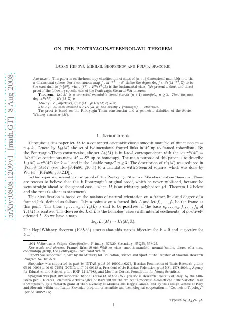
a r X i v :0808.1209v 1 [m a t h .G T ] 8 A u g 2008ON THE PONTRYAGIN-STEENROD-WU THEOREMDu ˇs an Repov ˇs ,Mikhail Skopenkov and Fulvia SpaggiariAbstract.This paper is on the homotopy classification of maps of (n +1)-dimensional manifolds into then -dimensional sphere.For a continuous map f :M n +1→S n define the degree deg f ∈H 1(M n +1;Z )to be the class dual to f ∗[S n ],where [S n ]∈H n (S n ;Z )is the fundamental class.We present a short and direct proof of the following specific case of the Pontryagin-Steenrod-Wu theorem:Theorem.Let M be a connected orientable closed smooth (n +1)-manifold,n ≥3.Then the map deg :πn (M )→H 1(M ;Z )is1-to-1(i.e.,bijective),if w 2(M )·ρ2H 2(M ;Z )=0;2-to-1(i.e.,each element α∈H 1(M ;Z )has exactly 2preimages)—otherwise.The proof is based on the Pontryagin-Thom construction and a geometric definition of the Stiefel–Whitney classes w i (M ).1.IntroductionThroughout this paper let M be a connected orientable closed smooth manifold of dimension m =n +k .Denote by L k (M )the set of k -dimensional framed links in M up to framed cobordism.By the Pontryagin-Thom construction,the set L k (M )is in 1-to-1correspondence with the set πn (M )=[M ;S n ]of continuous maps M →S n up to homotopy.The main purpose of this paper is to describe L 1(M )=πn (M )for k =1and in the ”stable range”n ≥3.The description of πn (M )was reduced in [Pon39][Ste47](see also [FoFu86;§30.3])to a calculation with Steenrod squares,which was done by Wu (cf.[FoFu86;§30.2.D]).In this paper we present a short proof of this Pontryagin-Steenrod-Wu classification theorem.There are reasons to believe that this is Pontryagin’s original proof,which he never published,because he went straight ahead to the general case –when M is an arbitrary polyhedron (cf.Theorem 1.2below and the remark after its statement).This classification is based on the notions of natural orientation on a framed link and degree of a framed link,defined as follows.Take a point x on a framed link L and let f 1,...,f n be the frame at this point.The basis e 1,...,e k of T x (L )is said to be positive ,if the basis e 1,...,e k ,f 1,...,f n of T x (M )is positive.The degree deg L of L is the homology class (with integral coefficients)of positively oriented L .So we have a mapdeg:L k (M )→H k (M ;Z ).The Hopf-Whitney theorem (1932-35)asserts that this map is bijective for k =0and surjective for k =1.2 D.REPOVˇS,M.SKOPENKOV AND F.SPAGGIARITheorem1.1.(a)Let M be a connected orientable closed smooth(n+1)-manifold,n≥3.The degree map deg:L1(M)→H1(M;Z)is1-to-1(i.e.,bijective),if w2(M)·ρ2H2(M;Z)=0;2-to-1(i.e.,each elementα∈H1(M;Z)has exactly2preimages)—otherwise.(b)Let M be a connected orientable closed smooth(n+2)-manifold,n≥3.Then an elementαlies in the image of deg:L2(M)→H2(M;Z)if and only if w2(M)·ρ2α=0.Here·is the multiplication H k(M;Z/2Z)×H k(M;Z/2Z)→Z/2Z andρ2:Z→Z/2Z is reduction modulo2.However,in the proof of Theorem1.1it is convenient to replace the cohomological Stiefel-Whitney classes by their homological duals.These classes are denoted by the same letters w i and¯w i, and their geometric definition(equivalent to other definitions)is recalled below.Then·in the above (and in all the below)formulae is to be understood as the intersection product H i(M)×H j(M)→H i+j−m(M).Notice that the conditionρ2β·w2(M)=0in case(a)of Theorem1.1cannot be replaced by w2(M)=0(e.g.,for M=R P4).Theorem1.2(Pontryagin).(a)Let M3be a connected orientable closed smooth3-manifold.Then for eachα∈H1(M3;Z)there is a1-1correspondence between the sets deg−1αand Z2d(α),where d(α) is the divisibility of the projection ofαto the free part of H1(M3;Z).(b)Let M be an orientable closed smooth4-manifold.Then an elementαlies in the image of deg:L2(M)→H2(M;Z)if and only ifα·α=0.Theorem1.2.b can be proved analogously to our proof of Theorem1.1.b below.Our methods can be used to prove Theorem1.2.a which was stated without proof in[Pon39].In fact,Theorem1.2.a was not included in[Pon39](published in English),but only in the abstract(published in Russian), without any indication of its proof.A short geometric proof of this result is published,for example,in [CRS07].2.Geometric definition of homology Stiefel-Whitney classesTake a general position system of s smooth tangent vectorfields on M.LetΣ⊂M be the set of points at which these vectorfields are not linearly independent.By transversality[DNF79;§10.3],Σis a pseudomanifold in M.The Stiefel-Whitney class w m+1−s(L)∈H s−1(M;Z/2Z)is the class of the pseudomanifoldΣ(this is thefirst obstruction to existence of a linear independent system of s tangent vectorfields on M).This definition can be easily generalized to the case when tangent vectorfields in T M are replaced by vectorfields in an arbitrary vector bundle with the base M.If L⊂M is a submanifold,then such classes for the normal bundle of L in M and for the restriction of T M to L are denoted by¯w2(L)and w2(M)|L,respectively.We will also use relative versions of these classes.For example,suppose that L⊂M is an l-submanifold with boundary and a system f of m−l−1linearly independent normal vectorfields is given on∂L.Then we can extend f to an arbitrary general position system of normal vectorfields on L.Define¯w2(L,f)∈H l−2(L;Z/2Z)to be the class of the(l−2)-pseudomanifold,on which these extended vectorfields are not linearly independent(this is thefirst obstruction to extension of f to a linear independent system on L).We will omit f from the notation,if no confusion could arise.3.Proof of Theorem1.1.bTake anyα∈H2(M;Z).Realizeαby an orientable2-submanifold L⊂M.Clearly,α∈Im deg if and only if L can be framed(for some choice of L).We may assume that L is connected.Indeed,if some disconnected L can be framed,then the submanifold,which is the connected sum of all connected components of L,can also be framed and realizes the same homological class.In this paragraph we show that L can be framed if and only if¯w2(L)=0.By the definition of ¯w2(L)this condition is necessary.In order to prove the sufficiency assume that¯w2(L)=0.Since n≥3 and dim L=2,it follows that there is an orthonormal system of vectorfields f1,...,f n−1which are normal to L.Since L2and M n+2are orientable,it follows that the normal bundle to L is orientable. Fix an orientation of this bundle.Taking a unit vectorfield f n ortogonal to f1,...,f n−1and such thatON THE PONTRYAGIN-STEENROD-WU THEOREM3 the basis f1,...,f n is positive(with respect to the specified orientation of the bundle),we obtain the required framing.Now the theorem follows from the equalities¯w2(L)=w2(M)|L=w2(M)·[L]=w2(M)·ρ2α.Here thefirst equality follows by the Wu formula of Stiefel-Whitney classes of the sum of two bundles: w2(M)|L=w2(L)+w1(L)·¯w1(L)+¯w2(L),in which w2(L)=w1(L)=0because L is an orientable 2-manifold(thefirst equality can also be proved directly).The second equality follows by the above geometric definition because L is connected(we identify H0(L;Z/2Z)∼=Z/2Z∼=H0(M;Z/2Z)).4.Proof of Theorem1.1.aTake an elementα∈H1(M;Z).Let L1,L2⊂M be a pair of framed1-submanifolds such that deg L1=deg L2.Denote by[L1],[L2]∈L1(M)their classes.Since L1and L2are homologous, it follows by general position that there is an embedded2-dimensional cobordism L⊂M×I(not framed)between them:∂L=L1⊔L2.Clearly,[L1]=[L2]if and only if for some L the framing of∂L extends to L.Assume further that L is connected.Let us show that the framing of∂L extends to that of L if and only if¯w2(L)=0.By definition of the relative Stiefel-Whitney classes this condition is necessary.Let us prove the sufficiency.Assume that¯w2(L)=0.Since n≥3and dim L=2,it follows that the orthonormal system of thefirst n−1 vectorfields of the framing of∂L extends to L.Since L and M×I are orientable,and L1,L2are naturally orientable,it follows that there is an orientation of the normal bundle of L in M×I restricted to the given orientations on L1and L2.So we can add one more unit vectorfield to the constructed ortonormal system on L to obtain a positive basis at each point of L(with respect to the specified orientation of L).So the required extension of the framing of∂L to L has been constructed.Completion of the proof of Theorem1.1.a in the case when w2(M)·ρ2H2(M,Z)=0.If ¯w2(L)=0then there is nothing to prove.Assume now that¯w2(L)=1.Here¯w2(L)∈H0(L;Z/2Z)∼= Z/2Z,because L is connected.Further we identify all groups H0(X;Z/2Z)isomorphic to Z/2Z with Z/2Z.Let us construct a new cobordism L′between L1and L2such that¯w2(L′)=0.Take an element β∈H2(M;Z)such that w2(M)·ρ2β=1.Let K be a connected orientable general position2-submanifold realizing the classβ.We may assume that K⊂M×12is a submanifold realizing the class w2(M),thefirst equality follows from geometricdefinition above.Put L′=L♯K(L∩K=∅by general position).By Claim4.1below¯w2(L′)=¯w2(L)+¯w2(K)=0,and this case of the theorem is proved.Claim4.1.Suppose that K2,L2⊂M n+2is a pair of disjoint connected orientable submanifolds and a frame of K and L is given on∂K and∂L,respectively.Then¯w2(K♯L)=¯w2(K)+¯w2(L),where the groups H0(X;Z/2Z)are identified with Z/2Z for X=K♯L,K and L.Proof of Claim4.1.Take a pair of small2-disks k⊂K and l⊂L.Let kl∼=S1×I be a narrow tube such that∂kl=∂k⊔∂l and kl is tangent to both disks k and l.Fix a trivial frame of k and l(and, consequently,of∂k and∂l).By the above geometric definition it follows easily that¯w2(K♯L)=¯w2(K−k)+¯w2(kl)+¯w2(L−l). On the other hand,one can check analogously that¯w2(K)=¯w2(K−k)+¯w2(k)and¯w2(L)=¯w2(L−l)+¯w2(l).Since¯w2(kl)=¯w2(k)=¯w2(l)=0,it follows that¯w2(K♯L)=¯w2(K)+¯w2(L). Completion of the proof of Theorem1.1.a in the case when w2(M)·ρ2H2(M,Z)=0.It suffices to show that forfixed[L1]the map[L2]→w2(L)is well-defined and is a bijection deg−1α→Z/2Z.Let us prove that the map is well-defined.Let L′1and L′2be a pair of framed submanifolds of M framed cobordant to L1and L2respectively.Let L′be a(not framed)cobordism between them.It suffices to prove that w2(L)=w2(L′)in case when L1and L′1,L2and L′2,L and L′are in general position.4 D.REPOVˇS,M.SKOPENKOV AND F.SPAGGIARIAssume that L1,L′1⊂M×1,L2,L′2⊂M×0and L,L′⊂M×[0,1].Change the sign of thefirst vectorfield belonging to the framings of L′1and L′2.Denote the obtained framed submanifolds by−L′1 and−L′2,respectively.Denote by¯w2(−L′)the relative Stiefel-Whitney class of L with the reversed framing of∂L′.Then ¯w2(−L′)=−¯w2(L′).Further,both L1⊔(−L′1)and L2⊔(−L′2)are framed cobordant to zero,i.e.to an empty submanifold.Let L+⊂M×[1,+∞)and L−⊂M×(−∞,0]be the corresponding framed cobordisms.Then¯w2(L+)=¯w2(L−)=0.By general position L∩L′=∅.Denote by K=L∪L+∪L′∪L−By the above geometric definition it follows easily that¯w2(K)=¯w2(L)+¯w2(L+)+¯w2(−L′)+¯w2(L−)=¯w2(L)−¯w2(L′).It suffices to show that¯w2(K)=0.Letβbe the cohomological class of image of K under the projection M×R→M.Analogously to the proof of the previous case of the theorem we see that ¯w2(K)=¯w2(M)·ρ2β=0,hence w2(L)=w2(L′)and our map deg−1α→Z/2Z is well-defined.Now let us prove that our map is injective.It suffices to show that if L′2is a framed1-submanifold and L′is a connected2-dimensional embedded cobordism(not framed)between L1and L′2such that ¯w2(L)=¯w2(L′),then[L2]=[L′2].Indeed,we may assume that L1⊂M×0,L2⊂M×1,L′2⊂M×(−1),L⊂M×[0,1]and L′⊂M×[−1,0].Then L∪L′is a cobordism between L2and L′2.By the above geometric definition it follows that¯w2(L∪L′)=¯w2(L)+¯w2(L′)=0,hence L∪L′can be framed.So our map deg−1α→Z/2Z is injective.Let us prove that our map is surjective.It suffices to show that some[L2]is mapped to1.Since M is orientable,it follows there exists a framing f1of L1.Fix a homeomorphism L1∼=S1.Denote by f1(x)the choice of the framing at the point x∈S1.Take a mapϕ:S1→SO(n)realizing a nonzero element ofπ1(SO(n))∼=Z/2Z(which is true because n≥3).Define a new framing f2of L1 by the formula f2(x)=ϕ(x)f1(x).The obtained framed submanifold is the required submanifold L2.Indeed,take L=L1×I.Then ¯w2(L)=1.Indeed,assume the converse.Then the frames of L1and L2can be extended to the frame of L1×I.This frame gives the homotopy betweenϕand the constant map in SO(n),which contradicts the choice ofϕ.This contradiction completes the proof of Theorem1.1.a.AcknowledgmentsWe thank A.B.Skopenkov and the referee for comments and suggestions.References[CRS07]M.Cencelj,D.Repovˇs and M.Skopenkov,Classification of framed links in3–manifolds,Proc.Indian Acad.Sci.(Math.Sci.)117:3(2007),301–306,arXiv:math-gt/0705.4166.[DNF79] B.A.Dubrovin,S.P.Novikov and A.T.Fomenko,Modern geometry:Methods and applications,Nauka, Moscow,1979.(in Russian)[FoFu89]A.T.Fomenko and D.B.Fuchs,A course in homotopy theory,Nauka,Moscow,1989.(in Russian)[Pon39]L.S.Pontryagin,Homologies in compact Lie groups,Mat.Sbornik6(1939),no.3,389–422.[Pon76]L.S.Pontryagin,Smooth manifolds and their application to homotopy theory,Nauka,Moscow,1976.(in Russian)[Ste47]N.E.Steenrod,Products of cocycles and extensions of mappings,Ann.of Math.(2)48(1947),290–320.Institute for Mathematics,Physics and Mechanics,University of Ljubljana,P.O.Box2964,1001 Ljubljana,Slovenia.e-mail:dusan.repovs@uni-lj.siDepartment of Differential Geometry,Faculty of Mechanics and Mathematics,Moscow State Uni-versity,Moscow,Russia119992.e-mail:skopenkov@rambler.ruDipartimento di Matematica,Universita‘di Modena e Reggio Emilia,via Campi213/B,41100Modena, Italy.e-mail:spaggiari.fulvia@unimo.ita r X i v :0808.1209v 1 [m a t h .G T ] 8 A u g 2008(n +1)nf :M n +1→S ndeg f ∈H 1(M ;Z )f ∗[S n ][S n ]∈H n (S n ;Z )M(n +1)n ≥3deg :πn (M )→H 1(M ;Z )w 2(M )·ρ2H 2(M ;Z )=0α∈H 1(M ;Z )w i (M )Mn +kL k (M )kML k (M )πn (M )=[M ;S n]M →S nL k (M )=πn (M )k =1n ≥3L k (M )MMxLf 1,...,f ne 1,...,e kT x (L )e 1,...,e k ,f 1,...,f n T x (M )deg LLLdeg :L k (M )→H k (M ;Z ).k =0k =1M(n +1)n ≥3deg :L 1(M )→H 1(M ;Z )w 2(M )·ρ2H 2(M ;Z )=0α∈H 1(M ;Z )M(n +2)n ≥3αdeg :L 2(M )→H 2(M ;Z )ρ2α·w 2(M )=0·H k (M ;Z 2)×H k (M ;Z 2)→Z 2w i¯w i·H i (M )×H j (M )→H i +j −m (M )ρ2β·w2(M)=0w2(M)=0M=R P4M3α∈H1(M3;Z)deg−1αZ2d(α)d(α)αH1(M3;Z)Mαdeg:L2(M)→H2(M;Z)α·α=0s MΣ⊂MΣM w n+2−s(L)∈H s−1(M;Z2)Σs MMM L⊂ML M T M L¯w i(L)w i(M)|LL⊂M×I lL1L2f∂L=L1∪L2m−l−1L¯w2(L,f)∈H l−2(L;Z2)(l−2)∂L L fα∈H2(M;Z)αLα∈Im degL LL LαL LL¯w2(L)=0¯w2(L)=0Lf1,...,f n−1n≥3dim L=2L2M n+2L Mf1,...,f n−1f nL¯w2(L)=w2(M)|L=w2(M)·[L]=w2(M)·ρ2α.Z2H0(X;Z2) Z2w2(M)|L=w2(L)+w1(L)·¯w1(L)+¯w2(L)w2(L)=w1(L)=0LLLα∈H1(M;Z)L i deg L i=αL1,L2⊂M deg L1= deg L2=α[L1][L2]L1(M)L1L2L⊂M×I,∂L=L1⊔L2.[L1]=[L2]L∂LL M L∂L L¯w2(L)=0¯w2(L)=0n−1L n≥3dim L=2 L M×I L1L2L L1L2n−1LLw2(M)·ρ2H2(M,Z)=0L1L2L¯w2(L)=0¯w2(L)=1¯w2(L)∈H0(L;Z2)∼=Z2LL′L1L2¯w2(L′)=0β∈H2(M;Z)w2(M)·ρ2β=1K⊂M×1¯w2(−L′)L′∂L′¯w2(−L′)=−¯w2(L′)L1⊔(−L′1)L2⊔(−L′2)L+⊂M×[1,+∞)L−⊂M×(−∞,0]¯w2(L+)=¯w2(L−)=0L∩L′=∅K=L∪L+∪L′∪L−¯w2(K)=¯w2(L)+¯w2(L+)+¯w2(−L′)+¯w2(L−)=¯w2(L)−¯w2(L′).w2(K)=0K M M×R→MβK¯w2(K)=¯w2(M)·ρ2β=0[L2]→w2(L)L′2L′L1L′2¯w2(L)=¯w2(L′) [L2]=[L′2]L1⊂M×0L2⊂M×1L′2⊂M×(−1)L⊂M×[0,1] L′⊂M×[−1,0]L∪L′L2L′2¯w2(L∪L′)=¯w2(L)+¯w2(L′)=0[L2]→w2(L)[L2] 1L1∼=S1Mf1L1f1(x)x∈S1ϕ:S1→SO(n)π1(SO(n))∼=Z2n≥3f2L1f2(x)=ϕ(x)f1(x)L2L1f2L=L1×I¯w2(L)=1f1f2L1×IϕS1→SO(n)ϕ。

写给那些喜欢数学和不喜欢数学的人们写给那些了解数学家和不了解数学家的人们Heroes in My HeartEdited by ukim贰·作者说明这是我在北大未名bbs连载的66篇文章，讲的是数学家们的故事。

从第一次发文到现在，已经将近三个月。

在davibaby的帮助下，把这些东西编成这么一个小册子，和bbs上的版本相比，这里的错别字要明显的少了，很多数学家的名字后面还加了中文的译名，不过，我还是想尽量保留bbs上的风格，从一开始的发信日期到最后的签名档，都作了保留。

希望大家喜欢。

叁·开篇辞发信人: ukim (我没有理想), 信区: Mathematics标题: 从今天开始连载数学家们的故事发信站: 北大未名站(2002年04月06日14:20:15 星期六), 转信给那些喜欢数学和不喜欢数学的人们给那些了解数学家和不了解数学家的人们在北大混了四年，一事无成；在未名上bbs也呆了快一年了，制造了几千篇的垃圾。

要毕业的人想法总是奇怪的，譬如说竟然真的要正经的写几篇文章了。

最初写成这些东西的时候，我发给了几个朋友，一个学数学的师弟说他很感动，一个非数学系的mm说她后悔当初没有选数学系。

无论怎样，他们能这样子讲，我很感动，这是发自内心的那种。

现在的打算是每天贴2-3个故事，一直到欧毕业那天。

很多事情难免有些tooold，这个我也没有办法，激动人心的事情毕竟只有那么多。

不多说了，真心的希望大家会喜欢，哪怕只有一点点的喜欢。

这些文字偶给了一个名字，叫做我心目中的英雄--- Heroes in My Heart美丽有两种一是深刻又动人的方程一是你泛着倦意淡淡的笑容肆·作者序发信人: ukim (我没有理想), 信区: Mathematics标题: Heroes in My Heart (序)发信站: 北大未名站(2002年04月06日14:23:24 星期六), 转信To MusicFor the Encouragement and Smiles She Gave Me 废话几句。

BZ反应||Belousov-Zhabotinski reaction, BZ reactionFPU问题||Fermi-Pasta-Ulam problem, FPU problemKBM方法||KBM method, Krylov-Bogoliubov-Mitropolskii method KS[动态]熵||Kolmogorov-Sinai entropy, KS entropyKdV 方程||KdV equationU形管||U-tubeWKB方法||WKB method, Wentzel-Kramers-Brillouin method[彻]体力||body force[单]元||element[第二类]拉格朗日方程||Lagrange equation [of the second kind] [叠栅]云纹||moiré fringe; 物理学称“叠栅条纹”。

[叠栅]云纹法||moiré method[抗]剪切角||angle of shear resistance[可]变形体||deformable body[钱]币状裂纹||penny-shape crack[映]象||image[圆]筒||cylinder[圆]柱壳||cylindrical shell[转]轴||shaft[转动]瞬心||instantaneous center [of rotation][转动]瞬轴||instantaneous axis [of rotation][状]态变量||state variable[状]态空间||state space[自]适应网格||[self-]adaptive meshＣ0连续问题||C0-continuous problemＣ1连续问题||C1-continuous problemＣＦＬ条件||Courant-Friedrichs-Lewy condition, CFL condition ＨＲＲ场||Hutchinson-Rice-Rosengren fieldＪ积分||J-integralＪ阻力曲线||J-resistance curveＫＡＭ定理||Kolgomorov-Arnol'd-Moser theorem, KAM theoremＫＡＭ环面||KAM torusｈ收敛||h-convergenceｐ收敛||p-convergenceπ定理||Buckingham theorem, pi theorem阿尔曼西应变||Almansis strain阿尔文波||Alfven wave阿基米德原理||Archimedes principle阿诺德舌[头]||Arnol'd tongue阿佩尔方程||Appel equation阿特伍德机||Atwood machine埃克曼边界层||Ekman boundary layer埃克曼流||Ekman flow埃克曼数||Ekman number埃克特数||Eckert number埃农吸引子||Henon attractor艾里应力函数||Airy stress function鞍点||saddle [point]鞍结分岔||saddle-node bifurcation安定[性]理论||shake-down theory安全寿命||safe life安全系数||safety factor安全裕度||safety margin暗条纹||dark fringe奥尔-索末菲方程||Orr-Sommerfeld equation奥辛流||Oseen flow奥伊洛特模型||Oldroyd model八面体剪应变||octohedral shear strain八面体剪应力||octohedral shear stress八面体剪应力理论||octohedral shear stress theory巴塞特力||Basset force白光散斑法||white-light speckle method摆||pendulum摆振||shimmy板||plate板块法||panel method板元||plate element半导体应变计||semiconductor strain gage半峰宽度||half-peak width半解析法||semi-analytical method半逆解法||semi-inverse method半频进动||half frequency precession半向同性张量||hemitropic tensor半隐格式||semi-implicit scheme薄壁杆||thin-walled bar薄壁梁||thin-walled beam薄壁筒||thin-walled cylinder薄膜比拟||membrane analogy薄翼理论||thin-airfoil theory保单调差分格式||monotonicity preserving difference scheme 保守力||conservative force保守系||conservative system爆发||blow up爆高||height of burst爆轰||detonation; 又称“爆震”。

导致Unruh-Hawking效应与可延拓出分叉Killing视界的充分条件张靖仪;杨锦波【摘要】文章回顾了“导致Hawking效应的普遍坐标变换”一文中产生Unruh-Hawking效应的条件,对这些条件的作用进行了梳理.基于同样的方法,作者找到了能导致可延拓分叉Killing视界的充分条件并做出了证明.新的条件原则上也可以把非时轴正交的情况包括进来.由于可延拓分叉Killing视界普遍具有非零的表面引力,因此,也可以说这些新条件是导致Unruh-Hawking效应的充分条件.最后以极端RN黑洞为例,讨论了极端Killing视界的情况.【期刊名称】《广州大学学报（自然科学版）》【年(卷),期】2017(016)002【总页数】5页(P9-13)【关键词】分叉Killing视界;非零表面引力;Unruh-Hawking效应;极端视界【作者】张靖仪;杨锦波【作者单位】广州大学天体物理中心,广东广州510006;广州大学天体物理中心,广东广州510006【正文语种】中文【中图分类】O412.1Rindler参考系的Unruh效应与黑洞的Hawking辐射的发现已经几十年了，它们的发现令黑洞力学四定律与热力学四定律的“形似”变为“神似” [1-2].人们从不同的角度出发去理解它们，有的从弯曲时空量子场论出发，证明了这种效应是分叉Killing视界的一个普适的性质[3-4]；有的认为虽然已经确定了视界普遍导致这种效应，但是其统计物理的根源尚未得到很好的理解[5-7]; 它同时还有其他物理上很新奇的想法的来源.例如，一个研究有限温度场论的非常有意义的工具——桂氏时空，也是受到这方面研究的启发提出来的[8-9].分叉Killing视界跟黑洞热力学第零定律——表面引力为常数有很大的关系.可以证明，分叉Killing视界的表面引力必定为常数，反过来，表面引力为常数的Killing 视界虽然不一定就是分叉Killing视界，但总可以延拓出一个分叉Killing视界[10]. 此外，WALD还证明了黑洞的熵可以视为微分同胚不变的引力理论对分叉Killing视界的Noether荷[11].可见分叉Killing视界应与黑洞热力学有很深的关系.黑洞的Hawking辐射引发了信息佯谬[12].现在基于全息原理的论证，大部分物理学家都相信Hawking辐射的过程是幺正的，但是不清楚信息释放的机制，一般都认为Hawking原来的计算忽略了出射Hawking辐射粒子与剩下的黑洞的微观态的关联[13].考虑了这一关联之后，幺正性就不会遭到破坏，但是这个考虑又引起了晚期黑洞会不会在视界形成Firewall的争论[14].在这场争论中，MADECENA等[15]提出了ER=EPR的猜想，它断言几何上的Einstein-Rosen桥时空构型跟量子的EPR纠缠对是等价的，例如，Schwarzchild-AdS的最大延拓正好可以在全息原理的意义上跟边界上的热纠缠态对应起来.这个想法起码能在特定的拓扑场论中以某种方式实现[16].随后更加激进的猜想——复杂度-体积对应乃至复杂度-作用量对应也被提出来[17-18].有趣的是，他们所谈的不可穿越虫洞——Einstein-Rosen桥实际上也是分叉Killing 视界的喉部.从这点来看，按照文献[3-4]的结果，起码可以认为ER=EPR在弯曲时空量子场论的层次上是成立的.文献[7]在寻找到Unruh-Hawking效应的统计物理根源这一方向上做出了努力.该文认为时空变量分离变量形式的坐标变换扮演了很重要的角色，地位可能相当于统计物理中的分子混沌假设.只要再提一些物理上合理的要求，可以证明，分离变量型的坐标变换会导致Unruh-Hawking效应.然而这些条件，有些是对坐标系的要求，有些又是对时空的要求，但并没有区分得很清楚.本文希望能进一步理清文献[7]所提条件的含义，进一步讨论它们和分叉Killing视界的关系，找出导致Hawking效应的充分条件.针对线元ds2=-G0dT2+G1dX2+G2dY2+G3dZ2, 文献[7]给出了能导致Hawking辐射的普遍坐标变换:①坐标系变换采取分离变量的形式且f1(x),f2(x),g1(t),g2(t)全都不为常数；②新时空时轴正交③新时空稳态且④满足初条件t=0时，T=0.这4个条件将会把坐标变换的形式限制成条件1构造了一个坐标系变换，但是坐标系变换是可以很随意的，取什么样的坐标变换都可以，初看是一个平凡的条件.条件4不怎么重要，只是个原点选择的问题.实质性的是条件3.条件3该分3个方面看.首先是要求新时空稳态，也就是说时空中存在类时Killing矢量场.其次是把它的积分曲线的参数用作时间坐标t，则可定义Killing矢量场的适配坐标系.在这个坐标系中，自动会有G3=0，粗略地看，这个要求似乎也很平凡.但它配合同样也是看上去很平凡的条件1就不平凡了，它们在一起相当于要求从坐标系{T,X,Y,Z}换到Killing矢量场的适配坐标系必须具有分离变量的形式.最后，条件3中最强的要求是G1=0.一般而言，度规分量与t无关只在适配坐标系中成立，换了其它坐标系就不一定成立.可见条件3还对其它坐标系中的度规分量提出了要求.而这个要求会对G0，G1做出限制，使它们满足一定的关系.它可以等价地理解为对这2个要求：(dT)a(dT)a和(dX)a(dX)a对Killing 矢量场的李导数为零.条件2限制太强，把Kerr一类的黑洞都排除在外，这其实可以改进.重要的是要挑出一个跟Killing矢量场垂直的方向.本节将用文献[7]中的技术，重新研究什么是可延拓出分叉Killing视界的充分条件.给定一个时空，时空里存在标量场r(可以据此定出时空分层)与类时Killing矢量场a, 它们满足:① aar=0.于是可以选定超曲面r=rc,由于 a总是切于超曲面，所以超曲面r=rc里总有 a的积分曲线.任意指定一条，再让rc发生变动，就得到一个以rc为参数的 a 积分曲线族，它张成一个二维子流形.二维子流形上的坐标可以自然地取为r和 a 积分曲线的参数η,并使得它满足，这个二维流形上的诱导度规为显然，aa和arar都不会是η的函数.②用η和r再进一步构造如下形式的标量场T,R其中， 1不能全局为零.要求它们满足如下条件可以证明存在常数c，使得(dT)a(dT)a+c2(dR)a(dR)a=0和L(T2-c2R2)=0成立.再进一步，如果(dT)a(dT)a作为T和R函数，在包括T=R=0的开集上满足-∞<(dT)a(dT)a<0,则可延拓出分叉Killing视界.下面给出证明过程.由T和R的构造可知为了简化公式，定义gTT=(dT)a(dT)a, gRR=(dR)a(dR)a, gηη=(dη)a(dη)a,grr=(dr)a(dr)a.于是因为1(η)不能全局为零,所以从公式(10)可以导出公式(8)和公式(9)就是要求LgTT=LgRR=0,可以导出可见，和都是常数，而且是非零常数.非零是因为如果常数为零，就会有g0和g1为常数, 继而T和R的表达式，不能用来构成坐标变换.反之可以设0=w1g1和1=w0g0，其中w0,w1都是不为零的常数.这样就有gηη.再次运用公式(8)和公式(9)可以求出公式(14)又给出于是，有根据上式和 a类时,可以得出w0与w1必定同号，这样0=w1g1和1=w0g0还蕴含着,即为常数,不妨记为K.并且，式(19)可以推出于是f1=af0,其中a是任意非零常数.从式(15)可以得到配合,还可以知道L，更进一步，有w0与w1必定同号意味着是正的常数.还可以求出可见K必定是负的常数， a类时说明gηη<0.条件gTT=(dT)a(dT)a为有限负数是可以得到满足的.引进坐标变换ξ = ,那么dr, 二维面上的诱导线元关系式(22)变为再根据和gTT必定是个有限负数，有原来讨论的时候要求a是类时的，只占据了R2<0区域，即ξ>0的范围.而式(26)和式(27)则表示ξ→0时，有aa→0.ξ可以光滑地延拓到等于0和小于0的地方，分别对应R2=0和的区域.在T-R平面上，代表和根直线，可见它就是分叉Killing 视界.命题得证.实际上对gTT在T=R=0附近的有限性要求暗示人们，即使坐标变换采取时空变量分离、时间部分作为双曲函数出现的形式，也不一定能延拓出分叉Killing视界，因而不一定有非零的表面引力.以RN黑洞为例，分极端情况和非极端情况讨论,以此来说明(dT)a(dT)a的重要性.给出RN黑洞的线元表达式视界位置由方程r2-2Mr+Q2=0决定.先讨论非极端黑洞，有r+≠r-，于是线元可以写为引入坐标变换其中则有其中如果选择，那么，而且在r=r+处是解析的.T,R可以延拓到T2-R2<0的区域以外.而这个ω的选择正好就是外视界r=r+的表面引力.对内视界也一样，如果选择,则G(r)在r=r-处解析.现在再来讨论极端RN黑洞，这时r+=r-=M，于是线元表达式是引入类似的坐标变换其中，将得到ds2=G(r)(-dT2+dR2)+r(T,R)2dΩ2其中r作为T,R的函数由下式决定无论如何选择ω,G(r)在r=M处的奇异性都无法消去，但是r=M对极端RN黑洞而言只是一个坐标奇性，这说明了坐标系{T,R}只能覆盖到T2-R2<0的区域，它没有办法做延拓.文献[7]提及的4个条件，极端RN黑洞都能满足，确实如同证明所表现的那样一定可以找到该文献中提到的特定的坐标变换:T=f(r)sinh(ωt),R=f(r)·cosh(ωt),然而极端RN黑洞的表面引力为0，意味着在极端RN黑洞的时空中不存在Hawking辐射(但可以有粒子对产生[19]).也就是说这种形式的坐标系变换并不如原来想象中那样会导致Hawking辐射.只有当可以延拓出分叉Killing视界的时候，才会有Unruh-Hawking效应.而要做到这点，就要在原来所提条件的基础上多加一个对(dT)a(dT)a解析性质的要求.可延拓出分叉Killing视界的充分条件是存在标量场r与类时Killing矢量场 a，满足 aar=0，并且可以利用它们去构造2个标量场T和R,满足要求L(dT)a(dT)a=L(dR)a(dR)a=(dT)a(dR)a=0，和要求(dT)a(dT)a作为T和R的函数在T=R=0附近有限.aar=0和L(dT)a(dT)a=L(dR)a(dR)a=(dT)a(dR)a=0 2个条件导致了L和个结果.这2个结果保证坐标变换中的η变量总会以双曲函数的形式出现.(dT)a(dT)a作为T和R的函数在T=R=0附近有限意味着总可以延拓出分叉Killing视界，于是总有一个非零的表面引力.最后这点的要求必不可少，极端RN黑洞就是一个很好的例子.【相关文献】[1] HAWKING S W. Particle creation by black holes[J]. Commun Math Phys，1975，43: 199-220.[2] UNRUH W G, WEISS N. Acceleration radiation in interacting field theories[J]. Phys Rev D，1984，29: 1656-1662.[3] JACOBSON T. A note on Hartle-Hawking Vacua[J]. Phys Rev D, 1994, 50:6031-6032.[4] SANDERS K. On the construction of Hartle-Hawking-Israel states across a static bifurcate killing horizon[J]. Lett Math Phys, 2015, 105(4): 575-640.[5] 赵峥. 四维静态黎曼时空中的Hawking辐射[J]. 物理学报，1981，30: 1508-1518.ZHAO Z. Hawking radiation in four dimensional static Riemann spacetime[J]. Acta Phys Sin, 1981, 30: 1508-1518.[6] 刘辽. 费曼路径积分和霍金蒸发[J]. 物理学报，1982，31(4): 519-524.LIU L. Feynman’s Path-integral Method and Hawking evaporation[J]. Acta Phys Sin, 1982, 31(4): 519-524.[7] 赵峥. 导致Hawking效应的普遍坐标变换[J]. 物理学报，1990，39(11): 1854-1862.ZHAO Z. University coordinate transformation leading to Hawking effect[J]. Acta Phys Sin, 1990, 39(11): 1854-1862.[8] GUI Y X. Quantum field in η-ξ spacetime[J]. Phys Rev D，1990，42: 1988-1995.[9] GUI Y X. Fermion fields in η-ξ spacetime[J]. Phys Rev D，1992，45: 697-700.[10]RACZ I, WALD R M. Extensions of spacetimes with killing horizons[J]. Class Quantum Grav，1992，9(12): 2643-2656.[11]WALD R M. Black hole entropy is the noether charge[J]. Phys Rev D，1993，48:R3427-3431.[12]HAWKING S W. Breakdown of predictability in gravitational collapse[J]. Phys Rev D，1976，14: 2460-2473.[13]VERLINDE E, VERLINDE H. Black Hole entanglement and quantum errorcorrection[J/OL]. 2012,arXiv:1211.6913v1 [hep-th].[14]ALMHEIRI A, MAROLF D, POLCHINSKI J, et al. Black Holes: Complementary or firewalls[J/OL]. 2012,arXiv:1207.3123v4 [hep-th].[15]MALDACENA J, SUSSKIND L. Cool horizons for entangled black holes[J/OL].2013,arXiv:1306.0533v2 [hep-th].[16]BAEZ J C, VICARY J. Wormholes and Entanglement[J/OL]. 2014,arXiv:1401.3416v2[gr-qc].[17]SUSSKIND L. Entanglement is not enough[J/OL]. 2014,arXiv:1411.0690v1[hep-th].[18]BROWN A R, ROBERTS D A, SUSSKIND L. Complexity equals action[J/OL].2015,arXiv:1509.07876v1 [hep-th].[19]CHEN C M, KIM S P, LIN I C, et al. Spontaneous pair production in reissner-nordström Black Holes[J/OL]. 2012,arXiv:1202.3224v2 [hep-th].。

庞加莱猜想-前言Wir m\"ussen wissen! Wir werden wissen!(我们必须知道！我们必将知道！)—— David Hilbert两年前科学版举行过一次版聚，我报告了低维拓扑里面的一些问题和进展，其中有一半篇幅是关于Poincar\'e 猜想。

版聚后，flyleaf 要求大家回去后把自己所讲的内容发在版上。

当时我甚至已经开始写了一两段，但后来又搁置了。

主要是因为自己对于低维拓扑还是一个门外汉，写出来的东西难免有疏漏之处，不敢妄下笔。

两年过去，我对低维拓扑这门学科的了解比原先多了，说话的底气也就比原先足了。

另外，由于Clay 研究所的百万巨赏，近年来Poincar\'e 猜想频频在媒体上曝光；而且Perelman 最近的工作使数学家们有理由相信我们已经充分接近于这一猜想的最后解决。

所以大概会有很多人对Poincar\'e 猜想的来龙去脉感兴趣，我也好借机一偿两年来的宿愿。

现代科学的高速发展使各学科之间的鸿沟加大，不同学科之间难以互相理解，所以非数学专业的读者在阅读本文时可能会遇到一些困难。

但限于篇幅和文章的形式，我也不可能对很多东西详细解释。

一些最基本的拓扑概念如“流形”，我将在本文的附录中解释。

还有一些“同调群”、“基本群”之类的名词，读者见到时大可不去理会它们的确切含义。

我将尽量避免使用这一类的专业术语。

作者并非拓扑方面的专家，对下面要说的很多内容都是道听途说，只知其然而不知其所以然；作者更不善于写作，写出来的东东总会枯燥无味，难登大雅之堂。

凡此种种，还请读者诸君海涵。

问题的由来Consid\'erons maintenant une vari\'et\'e [ferm\'ee] $V$ \`a trois dimensions ... Est-il possible que le groupe fondamental de $V$ ser\'eduise \`a la substitution identique, et que pourtant $V$ ne soit pas simplement connexe?—— Henri Poincar\'e在拓扑学家的眼里，篮球、排球和乒乓球并没有什么不同，它们都同胚于三维空间中的球面S^2. (我们把n+1维欧氏空间中到原点距离为1的点的集合记作S^n，称为n维球面(sphere)。

Quasi-Normal Modes of Stars and Black HolesKostas D.KokkotasDepartment of Physics,Aristotle University of Thessaloniki,Thessaloniki54006,Greece.kokkotas@astro.auth.grhttp://www.astro.auth.gr/˜kokkotasandBernd G.SchmidtMax Planck Institute for Gravitational Physics,Albert Einstein Institute,D-14476Golm,Germany.bernd@aei-potsdam.mpg.dePublished16September1999/Articles/Volume2/1999-2kokkotasLiving Reviews in RelativityPublished by the Max Planck Institute for Gravitational PhysicsAlbert Einstein Institute,GermanyAbstractPerturbations of stars and black holes have been one of the main topics of relativistic astrophysics for the last few decades.They are of partic-ular importance today,because of their relevance to gravitational waveastronomy.In this review we present the theory of quasi-normal modes ofcompact objects from both the mathematical and astrophysical points ofview.The discussion includes perturbations of black holes(Schwarzschild,Reissner-Nordstr¨o m,Kerr and Kerr-Newman)and relativistic stars(non-rotating and slowly-rotating).The properties of the various families ofquasi-normal modes are described,and numerical techniques for calculat-ing quasi-normal modes reviewed.The successes,as well as the limits,of perturbation theory are presented,and its role in the emerging era ofnumerical relativity and supercomputers is discussed.c 1999Max-Planck-Gesellschaft and the authors.Further information on copyright is given at /Info/Copyright/.For permission to reproduce the article please contact livrev@aei-potsdam.mpg.de.Article AmendmentsOn author request a Living Reviews article can be amended to include errata and small additions to ensure that the most accurate and up-to-date infor-mation possible is provided.For detailed documentation of amendments, please go to the article’s online version at/Articles/Volume2/1999-2kokkotas/. Owing to the fact that a Living Reviews article can evolve over time,we recommend to cite the article as follows:Kokkotas,K.D.,and Schmidt,B.G.,“Quasi-Normal Modes of Stars and Black Holes”,Living Rev.Relativity,2,(1999),2.[Online Article]:cited on<date>, /Articles/Volume2/1999-2kokkotas/. The date in’cited on<date>’then uniquely identifies the version of the article you are referring to.3Quasi-Normal Modes of Stars and Black HolesContents1Introduction4 2Normal Modes–Quasi-Normal Modes–Resonances7 3Quasi-Normal Modes of Black Holes123.1Schwarzschild Black Holes (12)3.2Kerr Black Holes (17)3.3Stability and Completeness of Quasi-Normal Modes (20)4Quasi-Normal Modes of Relativistic Stars234.1Stellar Pulsations:The Theoretical Minimum (23)4.2Mode Analysis (26)4.2.1Families of Fluid Modes (26)4.2.2Families of Spacetime or w-Modes (30)4.3Stability (31)5Excitation and Detection of QNMs325.1Studies of Black Hole QNM Excitation (33)5.2Studies of Stellar QNM Excitation (34)5.3Detection of the QNM Ringing (37)5.4Parameter Estimation (39)6Numerical Techniques426.1Black Holes (42)6.1.1Evolving the Time Dependent Wave Equation (42)6.1.2Integration of the Time Independent Wave Equation (43)6.1.3WKB Methods (44)6.1.4The Method of Continued Fractions (44)6.2Relativistic Stars (45)7Where Are We Going?487.1Synergism Between Perturbation Theory and Numerical Relativity487.2Second Order Perturbations (48)7.3Mode Calculations (49)7.4The Detectors (49)8Acknowledgments50 9Appendix:Schr¨o dinger Equation Versus Wave Equation51Living Reviews in Relativity(1999-2)K.D.Kokkotas and B.G.Schmidt41IntroductionHelioseismology and asteroseismology are well known terms in classical astro-physics.From the beginning of the century the variability of Cepheids has been used for the accurate measurement of cosmic distances,while the variability of a number of stellar objects(RR Lyrae,Mira)has been associated with stel-lar oscillations.Observations of solar oscillations(with thousands of nonradial modes)have also revealed a wealth of information about the internal structure of the Sun[204].Practically every stellar object oscillates radially or nonradi-ally,and although there is great difficulty in observing such oscillations there are already results for various types of stars(O,B,...).All these types of pulsations of normal main sequence stars can be studied via Newtonian theory and they are of no importance for the forthcoming era of gravitational wave astronomy.The gravitational waves emitted by these stars are extremely weak and have very low frequencies(cf.for a discussion of the sun[70],and an im-portant new measurement of the sun’s quadrupole moment and its application in the measurement of the anomalous precession of Mercury’s perihelion[163]). This is not the case when we consider very compact stellar objects i.e.neutron stars and black holes.Their oscillations,produced mainly during the formation phase,can be strong enough to be detected by the gravitational wave detectors (LIGO,VIRGO,GEO600,SPHERE)which are under construction.In the framework of general relativity(GR)quasi-normal modes(QNM) arise,as perturbations(electromagnetic or gravitational)of stellar or black hole spacetimes.Due to the emission of gravitational waves there are no normal mode oscillations but instead the frequencies become“quasi-normal”(complex), with the real part representing the actual frequency of the oscillation and the imaginary part representing the damping.In this review we shall discuss the oscillations of neutron stars and black holes.The natural way to study these oscillations is by considering the linearized Einstein equations.Nevertheless,there has been recent work on nonlinear black hole perturbations[101,102,103,104,100]while,as yet nothing is known for nonlinear stellar oscillations in general relativity.The study of black hole perturbations was initiated by the pioneering work of Regge and Wheeler[173]in the late50s and was continued by Zerilli[212]. The perturbations of relativistic stars in GR werefirst studied in the late60s by Kip Thorne and his collaborators[202,198,199,200].The initial aim of Regge and Wheeler was to study the stability of a black hole to small perturbations and they did not try to connect these perturbations to astrophysics.In con-trast,for the case of relativistic stars,Thorne’s aim was to extend the known properties of Newtonian oscillation theory to general relativity,and to estimate the frequencies and the energy radiated as gravitational waves.QNMs werefirst pointed out by Vishveshwara[207]in calculations of the scattering of gravitational waves by a Schwarzschild black hole,while Press[164] coined the term quasi-normal frequencies.QNM oscillations have been found in perturbation calculations of particles falling into Schwarzschild[73]and Kerr black holes[76,80]and in the collapse of a star to form a black hole[66,67,68]. Living Reviews in Relativity(1999-2)5Quasi-Normal Modes of Stars and Black Holes Numerical investigations of the fully nonlinear equations of general relativity have provided results which agree with the results of perturbation calculations;in particular numerical studies of the head-on collision of two black holes [30,29](cf.Figure 1)and gravitational collapse to a Kerr hole [191].Recently,Price,Pullin and collaborators [170,31,101,28]have pushed forward the agreement between full nonlinear numerical results and results from perturbation theory for the collision of two black holes.This proves the power of the perturbation approach even in highly nonlinear problems while at the same time indicating its limits.In the concluding remarks of their pioneering paper on nonradial oscillations of neutron stars Thorne and Campollataro [202]described it as “just a modest introduction to a story which promises to be long,complicated and fascinating ”.The story has undoubtedly proved to be intriguing,and many authors have contributed to our present understanding of the pulsations of both black holes and neutron stars.Thirty years after these prophetic words by Thorne and Campollataro hundreds of papers have been written in an attempt to understand the stability,the characteristic frequencies and the mechanisms of excitation of these oscillations.Their relevance to the emission of gravitational waves was always the basic underlying reason of each study.An account of all this work will be attempted in the next sections hoping that the interested reader will find this review useful both as a guide to the literature and as an inspiration for future work on the open problems of the field.020406080100Time (M ADM )-0.3-0.2-0.10.00.10.20.3(l =2) Z e r i l l i F u n c t i o n Numerical solutionQNM fit Figure 1:QNM ringing after the head-on collision of two unequal mass black holes [29].The continuous line corresponds to the full nonlinear numerical calculation while the dotted line is a fit to the fundamental and first overtone QNM.In the next section we attempt to give a mathematical definition of QNMs.Living Reviews in Relativity (1999-2)K.D.Kokkotas and B.G.Schmidt6 The third and fourth section will be devoted to the study of the black hole and stellar QNMs.In thefifth section we discuss the excitation and observation of QNMs andfinally in the sixth section we will mention the more significant numerical techniques used in the study of QNMs.Living Reviews in Relativity(1999-2)7Quasi-Normal Modes of Stars and Black Holes 2Normal Modes–Quasi-Normal Modes–Res-onancesBefore discussing quasi-normal modes it is useful to remember what normal modes are!Compact classical linear oscillating systems such asfinite strings,mem-branes,or cavitiesfilled with electromagnetic radiation have preferred time harmonic states of motion(ωis real):χn(t,x)=e iωn tχn(x),n=1,2,3...,(1) if dissipation is neglected.(We assumeχto be some complex valuedfield.) There is generally an infinite collection of such periodic solutions,and the“gen-eral solution”can be expressed as a superposition,χ(t,x)=∞n=1a n e iωn tχn(x),(2)of such normal modes.The simplest example is a string of length L which isfixed at its ends.All such systems can be described by systems of partial differential equations of the type(χmay be a vector)∂χ∂t=Aχ,(3)where A is a linear operator acting only on the spatial variables.Because of thefiniteness of the system the time evolution is only determined if some boundary conditions are prescribed.The search for solutions periodic in time leads to a boundary value problem in the spatial variables.In simple cases it is of the Sturm-Liouville type.The treatment of such boundary value problems for differential equations played an important role in the development of Hilbert space techniques.A Hilbert space is chosen such that the differential operator becomes sym-metric.Due to the boundary conditions dictated by the physical problem,A becomes a self-adjoint operator on the appropriate Hilbert space and has a pure point spectrum.The eigenfunctions and eigenvalues determine the periodic solutions(1).The definition of self-adjointness is rather subtle from a physicist’s point of view since fairly complicated“domain issues”play an essential role.(See[43] where a mathematical exposition for physicists is given.)The wave equation modeling thefinite string has solutions of various degrees of differentiability. To describe all“realistic situations”,clearly C∞functions should be sufficient. Sometimes it may,however,also be convenient to consider more general solu-tions.From the mathematical point of view the collection of all smooth functions is not a natural setting to study the wave equation because sequences of solutionsLiving Reviews in Relativity(1999-2)K.D.Kokkotas and B.G.Schmidt8 exist which converge to non-smooth solutions.To establish such powerful state-ments like(2)one has to study the equation on certain subsets of the Hilbert space of square integrable functions.For“nice”equations it usually happens that the eigenfunctions are in fact analytic.They can then be used to gen-erate,for example,all smooth solutions by a pointwise converging series(2). The key point is that we need some mathematical sophistication to obtain the “completeness property”of the eigenfunctions.This picture of“normal modes”changes when we consider“open systems”which can lose energy to infinity.The simplest case are waves on an infinite string.The general solution of this problem isχ(t,x)=A(t−x)+B(t+x)(4) with“arbitrary”functions A and B.Which solutions should we study?Since we have all solutions,this is not a serious question.In more general cases, however,in which the general solution is not known,we have to select a certain class of solutions which we consider as relevant for the physical problem.Let us consider for the following discussion,as an example,a wave equation with a potential on the real line,∂2∂t2χ+ −∂2∂x2+V(x)χ=0.(5)Cauchy dataχ(0,x),∂tχ(0,x)which have two derivatives determine a unique twice differentiable solution.No boundary condition is needed at infinity to determine the time evolution of the data!This can be established by fairly simple PDE theory[116].There exist solutions for which the support of thefields are spatially compact, or–the other extreme–solutions with infinite total energy for which thefields grow at spatial infinity in a quite arbitrary way!From the point of view of physics smooth solutions with spatially compact support should be the relevant class–who cares what happens near infinity! Again it turns out that mathematically it is more convenient to study all solu-tions offinite total energy.Then the relevant operator is again self-adjoint,but now its spectrum is purely“continuous”.There are no eigenfunctions which are square integrable.Only“improper eigenfunctions”like plane waves exist.This expresses the fact that wefind a solution of the form(1)for any realωand by forming appropriate superpositions one can construct solutions which are “almost eigenfunctions”.(In the case V(x)≡0these are wave packets formed from plane waves.)These solutions are the analogs of normal modes for infinite systems.Let us now turn to the discussion of“quasi-normal modes”which are concep-tually different to normal modes.To define quasi-normal modes let us consider the wave equation(5)for potentials with V≥0which vanish for|x|>x0.Then in this case all solutions determined by data of compact support are bounded: |χ(t,x)|<C.We can use Laplace transformation techniques to represent such Living Reviews in Relativity(1999-2)9Quasi-Normal Modes of Stars and Black Holes solutions.The Laplace transformˆχ(s,x)(s>0real)of a solutionχ(t,x)isˆχ(s,x)= ∞0e−stχ(t,x)dt,(6) and satisfies the ordinary differential equations2ˆχ−ˆχ +Vˆχ=+sχ(0,x)+∂tχ(0,x),(7) wheres2ˆχ−ˆχ +Vˆχ=0(8) is the homogeneous equation.The boundedness ofχimplies thatˆχis analytic for positive,real s,and has an analytic continuation onto the complex half plane Re(s)>0.Which solutionˆχof this inhomogeneous equation gives the unique solution in spacetime determined by the data?There is no arbitrariness;only one of the Green functions for the inhomogeneous equation is correct!All Green functions can be constructed by the following well known method. Choose any two linearly independent solutions of the homogeneous equation f−(s,x)and f+(s,x),and defineG(s,x,x )=1W(s)f−(s,x )f+(s,x)(x <x),f−(s,x)f+(s,x )(x >x),(9)where W(s)is the Wronskian of f−and f+.If we denote the inhomogeneity of(7)by j,a solution of(7)isˆχ(s,x)= ∞−∞G(s,x,x )j(s,x )dx .(10) We still have to select a unique pair of solutions f−,f+.Here the information that the solution in spacetime is bounded can be used.The definition of the Laplace transform implies thatˆχis bounded as a function of x.Because the potential V vanishes for|x|>x0,the solutions of the homogeneous equation(8) for|x|>x0aref=e±sx.(11) The following pair of solutionsf+=e−sx for x>x0,f−=e+sx for x<−x0,(12) which is linearly independent for Re(s)>0,gives the unique Green function which defines a bounded solution for j of compact support.Note that for Re(s)>0the solution f+is exponentially decaying for large x and f−is expo-nentially decaying for small x.For small x however,f+will be a linear com-bination a(s)e−sx+b(s)e sx which will in general grow exponentially.Similar behavior is found for f−.Living Reviews in Relativity(1999-2)K.D.Kokkotas and B.G.Schmidt 10Quasi-Normal mode frequencies s n can be defined as those complex numbers for whichf +(s n ,x )=c (s n )f −(s n ,x ),(13)that is the two functions become linearly dependent,the Wronskian vanishes and the Green function is singular!The corresponding solutions f +(s n ,x )are called quasi eigenfunctions.Are there such numbers s n ?From the boundedness of the solution in space-time we know that the unique Green function must exist for Re (s )>0.Hence f +,f −are linearly independent for those values of s .However,as solutions f +,f −of the homogeneous equation (8)they have a unique continuation to the complex s plane.In [35]it is shown that for positive potentials with compact support there is always a countable number of zeros of the Wronskian with Re (s )<0.What is the mathematical and physical significance of the quasi-normal fre-quencies s n and the corresponding quasi-normal functions f +?First of all we should note that because of Re (s )<0the function f +grows exponentially for small and large x !The corresponding spacetime solution e s n t f +(s n ,x )is therefore not a physically relevant solution,unlike the normal modes.If one studies the inverse Laplace transformation and expresses χas a com-plex line integral (a >0),χ(t,x )=12πi +∞−∞e (a +is )t ˆχ(a +is,x )ds,(14)one can deform the path of the complex integration and show that the late time behavior of solutions can be approximated in finite parts of the space by a finite sum of the form χ(t,x )∼N n =1a n e (αn +iβn )t f +(s n ,x ).(15)Here we assume that Re (s n +1)<Re (s n )<0,s n =αn +iβn .The approxi-mation ∼means that if we choose x 0,x 1, and t 0then there exists a constant C (t 0,x 0,x 1, )such that χ(t,x )−N n =1a n e (αn +iβn )t f +(s n ,x ) ≤Ce (−|αN +1|+ )t (16)holds for t >t 0,x 0<x <x 1, >0with C (t 0,x 0,x 1, )independent of t .The constants a n depend only on the data [35]!This implies in particular that all solutions defined by data of compact support decay exponentially in time on spatially bounded regions.The generic leading order decay is determined by the quasi-normal mode frequency with the largest real part s 1,i.e.slowest damping.On finite intervals and for late times the solution is approximated by a finite sum of quasi eigenfunctions (15).It is presently unclear whether one can strengthen (16)to a statement like (2),a pointwise expansion of the late time solution in terms of quasi-normal Living Reviews in Relativity (1999-2)11Quasi-Normal Modes of Stars and Black Holes modes.For one particular potential(P¨o schl-Teller)this has been shown by Beyer[42].Let us now consider the case where the potential is positive for all x,but decays near infinity as happens for example for the wave equation on the static Schwarzschild spacetime.Data of compact support determine again solutions which are bounded[117].Hence we can proceed as before.Thefirst new point concerns the definitions of f±.It can be shown that the homogeneous equation(8)has for each real positive s a unique solution f+(s,x)such that lim x→∞(e sx f+(s,x))=1holds and correspondingly for f−.These functions are uniquely determined,define the correct Green function and have analytic continuations onto the complex half plane Re(s)>0.It is however quite complicated to get a good representation of these func-tions.If the point at infinity is not a regular singular point,we do not even get converging series expansions for f±.(This is particularly serious for values of s with negative real part because we expect exponential growth in x).The next new feature is that the analyticity properties of f±in the complex s plane depend on the decay of the potential.To obtain information about analytic continuation,even use of analyticity properties of the potential in x is made!Branch cuts may occur.Nevertheless in a lot of cases an infinite number of quasi-normal mode frequencies exists.The fact that the potential never vanishes may,however,destroy the expo-nential decay in time of the solutions and therefore the essential properties of the quasi-normal modes.This probably happens if the potential decays slower than exponentially.There is,however,the following way out:Suppose you want to study a solution determined by data of compact support from t=0to some largefinite time t=T.Up to this time the solution is–because of domain of dependence properties–completely independent of the potential for sufficiently large x.Hence we may see an exponential decay of the form(15)in a time range t1<t<T.This is the behavior seen in numerical calculations.The situation is similar in the case ofα-decay in quantum mechanics.A comparison of quasi-normal modes of wave equations and resonances in quantum theory can be found in the appendix,see section9.Living Reviews in Relativity(1999-2)K.D.Kokkotas and B.G.Schmidt123Quasi-Normal Modes of Black HolesOne of the most interesting aspects of gravitational wave detection will be the connection with the existence of black holes[201].Although there are presently several indirect ways of identifying black holes in the universe,gravitational waves emitted by an oscillating black hole will carry a uniquefingerprint which would lead to the direct identification of their existence.As we mentioned earlier,gravitational radiation from black hole oscillations exhibits certain characteristic frequencies which are independent of the pro-cesses giving rise to these oscillations.These“quasi-normal”frequencies are directly connected to the parameters of the black hole(mass,charge and angu-lar momentum)and for stellar mass black holes are expected to be inside the bandwidth of the constructed gravitational wave detectors.The perturbations of a Schwarzschild black hole reduce to a simple wave equation which has been studied extensively.The wave equation for the case of a Reissner-Nordstr¨o m black hole is more or less similar to the Schwarzschild case,but for Kerr one has to solve a system of coupled wave equations(one for the radial part and one for the angular part).For this reason the Kerr case has been studied less thoroughly.Finally,in the case of Kerr-Newman black holes we face the problem that the perturbations cannot be separated in their angular and radial parts and thus apart from special cases[124]the problem has not been studied at all.3.1Schwarzschild Black HolesThe study of perturbations of Schwarzschild black holes assumes a small per-turbation hµνon a static spherically symmetric background metricds2=g0µνdxµdxν=−e v(r)dt2+eλ(r)dr2+r2 dθ2+sin2θdφ2 ,(17) with the perturbed metric having the formgµν=g0µν+hµν,(18) which leads to a variation of the Einstein equations i.e.δGµν=4πδTµν.(19) By assuming a decomposition into tensor spherical harmonics for each hµνof the formχ(t,r,θ,φ)= mχ m(r,t)r Y m(θ,φ),(20)the perturbation problem is reduced to a single wave equation,for the func-tionχ m(r,t)(which is a combination of the various components of hµν).It should be pointed out that equation(20)is an expansion for scalar quantities only.From the10independent components of the hµνonly h tt,h tr,and h rr transform as scalars under rotations.The h tθ,h tφ,h rθ,and h rφtransform asLiving Reviews in Relativity(1999-2)13Quasi-Normal Modes of Stars and Black Holes components of two-vectors under rotations and can be expanded in a series of vector spherical harmonics while the components hθθ,hθφ,and hφφtransform as components of a2×2tensor and can be expanded in a series of tensor spher-ical harmonics(see[202,212,152]for details).There are two classes of vector spherical harmonics(polar and axial)which are build out of combinations of the Levi-Civita volume form and the gradient operator acting on the scalar spherical harmonics.The difference between the two families is their parity. Under the parity operatorπa spherical harmonic with index transforms as (−1) ,the polar class of perturbations transform under parity in the same way, as(−1) ,and the axial perturbations as(−1) +11.Finally,since we are dealing with spherically symmetric spacetimes the solution will be independent of m, thus this subscript can be omitted.The radial component of a perturbation outside the event horizon satisfies the following wave equation,∂2∂t χ + −∂2∂r∗+V (r)χ =0,(21)where r∗is the“tortoise”radial coordinate defined byr∗=r+2M log(r/2M−1),(22) and M is the mass of the black hole.For“axial”perturbationsV (r)= 1−2M r ( +1)r+2σMr(23)is the effective potential or(as it is known in the literature)Regge-Wheeler potential[173],which is a single potential barrier with a peak around r=3M, which is the location of the unstable photon orbit.The form(23)is true even if we consider scalar or electromagnetic testfields as perturbations.The parameter σtakes the values1for scalar perturbations,0for electromagnetic perturbations, and−3for gravitational perturbations and can be expressed asσ=1−s2,where s=0,1,2is the spin of the perturbingfield.For“polar”perturbations the effective potential was derived by Zerilli[212]and has the form V (r)= 1−2M r 2n2(n+1)r3+6n2Mr2+18nM2r+18M3r3(nr+3M)2,(24)1In the literature the polar perturbations are also called even-parity because they are characterized by their behavior under parity operations as discussed earlier,and in the same way the axial perturbations are called odd-parity.We will stick to the polar/axial terminology since there is a confusion with the definition of the parity operation,the reason is that to most people,the words“even”and“odd”imply that a mode transforms underπas(−1)2n or(−1)2n+1respectively(for n some integer).However only the polar modes with even have even parity and only axial modes with even have odd parity.If is odd,then polar modes have odd parity and axial modes have even parity.Another terminology is to call the polar perturbations spheroidal and the axial ones toroidal.This definition is coming from the study of stellar pulsations in Newtonian theory and represents the type offluid motions that each type of perturbation induces.Since we are dealing both with stars and black holes we will stick to the polar/axial terminology.Living Reviews in Relativity(1999-2)K.D.Kokkotas and B.G.Schmidt14where2n=( −1)( +2).(25) Chandrasekhar[54]has shown that one can transform the equation(21)for “axial”modes to the corresponding one for“polar”modes via a transforma-tion involving differential operations.It can also be shown that both forms are connected to the Bardeen-Press[38]perturbation equation derived via the Newman-Penrose formalism.The potential V (r∗)decays exponentially near the horizon,r∗→−∞,and as r−2∗for r∗→+∞.From the form of equation(21)it is evident that the study of black hole perturbations will follow the footsteps of the theory outlined in section2.Kay and Wald[117]have shown that solutions with data of compact sup-port are bounded.Hence we know that the time independent Green function G(s,r∗,r ∗)is analytic for Re(s)>0.The essential difficulty is now to obtain the solutions f±(cf.equation(10))of the equations2ˆχ−ˆχ +Vˆχ=0,(26) (prime denotes differentiation with respect to r∗)which satisfy for real,positives:f+∼e−sr∗for r∗→∞,f−∼e+r∗x for r∗→−∞.(27) To determine the quasi-normal modes we need the analytic continuations of these functions.As the horizon(r∗→∞)is a regular singular point of(26),a representation of f−(r∗,s)as a converging series exists.For M=12it reads:f−(r,s)=(r−1)s∞n=0a n(s)(r−1)n.(28)The series converges for all complex s and|r−1|<1[162].(The analytic extension of f−is investigated in[115].)The result is that f−has an extension to the complex s plane with poles only at negative real integers.The representation of f+is more complicated:Because infinity is a singular point no power series expansion like(28)exists.A representation coming from the iteration of the defining integral equation is given by Jensen and Candelas[115],see also[159]. It turns out that the continuation of f+has a branch cut Re(s)≤0due to the decay r−2for large r[115].The most extensive mathematical investigation of quasi-normal modes of the Schwarzschild solution is contained in the paper by Bachelot and Motet-Bachelot[35].Here the existence of an infinite number of quasi-normal modes is demonstrated.Truncating the potential(23)to make it of compact support leads to the estimate(16).The decay of solutions in time is not exponential because of the weak decay of the potential for large r.At late times,the quasi-normal oscillations are swamped by the radiative tail[166,167].This tail radiation is of interest in its Living Reviews in Relativity(1999-2)。