Compressing Sparse Tables using a Genetic Algorithm

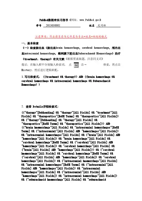
PubMed数据库实习指导（网址：）学号2013038081 姓名皮鸿林注意事项：作业请另存为文件名为专业+姓名+班级的格式一、基本检索（一）检索脑出血（脑出血brain hemorrhage，cerebral hemorrhage，颅内出血intracranial hemorrhage，蛛网膜下腔出血Subarachnoid Hemorrhage）治疗（treatment、therapy）有关文献（根据要求做题，注意同义词）提示：在输入框中分别输入检索词，点击→检索，再点击History，然后进行逻辑组配。

1.写出检索式： ((treatment OR therapy)) AND ((brain hemorrhage OR cerebral hemorrhage OR intracranial hemorrhage OR Subarachnoid Hemorrhage) )2．查看 Details详细检索式:(("therapy"[Subheading] OR "therapy"[All Fields] OR "treatment"[All Fields] OR "therapeutics"[MeSH Terms] OR "therapeutics"[All Fields]) OR ("therapy"[Subheading] OR "therapy"[All Fields] OR "therapeutics"[MeSH Terms] OR "therapeutics"[All Fields])) AND (("brain haemorrhage"[All Fields] OR "intracranial hemorrhages"[MeSH Terms] OR ("intracranial"[All Fields] AND "hemorrhages"[All Fields]) OR "intracranial hemorrhages"[All Fields] OR ("brain"[All Fields] AND "hemorrhage"[All Fields]) OR "brain hemorrhage"[All Fields] OR "cerebral hemorrhage"[MeSH Terms] OR ("cerebral"[All Fields] AND "hemorrhage"[All Fields]) OR "cerebral hemorrhage"[All Fields] OR ("brain"[All Fields] AND "hemorrhage"[All Fields])) OR ("cerebral haemorrhage"[All Fields] OR "cerebral hemorrhage"[MeSH Terms] OR ("cerebral"[All Fields] AND "hemorrhage"[All Fields]) OR "cerebral hemorrhage"[All Fields]) OR ("intracranial haemorrhage"[All Fields] OR "intracranial hemorrhages"[MeSH Terms] OR ("intracranial"[All Fields] AND "hemorrhages"[All Fields]) OR "intracranial hemorrhages"[All Fields] OR ("intracranial"[All Fields] AND "hemorrhage"[All Fields]) OR "intracranial hemorrhage"[All Fields]) OR ("subarachnoid haemorrhage"[All Fields] OR "subarachnoidhemorrhage"[MeSH Terms] OR ("subarachnoid"[All Fields] AND "hemorrhage"[All Fields]) OR "subarachnoid hemorrhage"[All Fields]))（二）检索骨折（fracture）的外科手术疗法（surgery）的近二年英文或者法文免费综述提示：点击Limits: 按要求的四个限制条件选择后，点击系统开始检索。

cofecha输出⽂件翻译[] Dendrochronology Program Library Run 9 Program COF 11:05 Wed 13 Jul 2011 Page 1 [] P R O G R A M C O F E C H A Version 6.06P 27954------------------------------------------------------------------------------------------------------------------------------------ QUALITY CONTROL AND DATING CHECK OF TREE-RING MEASUREMENTS树⽊年轮测量的质量控制和定年检查File of DATED series: 9.RWLCONTENTS:Part 1: Title page, options selected, summary, absent rings by series第1部分：标题页，已选项，总结，缺轮Part 2: Histogram of time spans第2部分：时间跨度直⽅图Part 3: Master series with sample depth and absent rings by year第3部分：主序列每年的样本和缺轮数量Part 4: Bar plot of Master Dating Series第4部分：主序列柱状图Part 5: Correlation by segment of each series with Master第5部分：每序列各段与主序列的相关性研究Part 6: Potential problems: low correlation, divergent year-to-year changes, absent rings, outliers 第6部分：潜在的问题：关联度低，年间发散变化，缺轮，异常值Part 7: Descriptive statistics第7部分：描述性统计Time span of Master dating series is 1815 to 2009 195 yearsContinuous time span is 1815 to 2009 195 yearsPortion with two or more series is 1816 to 2009 194 years*****************************************C* Number of dated series4 *C* 定年的样芯数量*O* Master series 1815 2009 195 yrs *O* 主序列*F* Total rings in all series 768 *F* 所有轮数*E* Total dated rings checked 767 *E* 被定年的轮数*C* Series intercorrelation .299 *C* 序列相关系数*H* Average mean sensitivity .195 *H* 平均敏感度*A* Segments, possible problems 26 *A* 可能有问题的部分数*** Mean length of series 192.0 *** 序列平均长度****************************************ABSENT RINGS listed by SERIES: (See Master Dating Series for absent rings listed by year) No ring measurements of zero value------------------------------------------------------------------------------------------------------------------------------------PART 6: POTENTIAL PROBLEMS: 第6部分：潜在的问题：关联度低，年间发散变化，缺轮，异常值08:08 Thu 14 Jul 2011 Page 5------------------------------------------------------------------------------------------------------------------------------------For each series with potential problems the following diagnostics may appear:检测出来的每个序列可能存在的潜在问题。

An Introduction to Categorical Data Analysis Using RBrett PresnellMarch28,2000AbstractThis document attempts to reproduce the examples and some of the exercises in An Introduction to Categor-ical Data Analysis[1]using the R statistical programming environment.Chapter0About This DocumentThis document attempts to reproduce the examples and some of the exercises in An Introduction to Categori-cal Data Analysis[1]using the R statistical programming environment.Numbering and titles of chapters will follow that of Agresti’s text,so if a particular example/analysis is of interest,it should not be hard tofind, assuming that it is here.Since R is particularly versatile,there are often a number of different ways to accomplish a task,and naturally this document can only demonstrate a limited number of possibilities.The reader is urged to explore other approaches on their own.In this regard it can be very helpful to read the online documentation for the various functions of R,as well as other tutorials.The helpfiles for many of the R functions used here are also included in the appendix for easy reference,but the online help system is definitely the preferred way to access this information.It is also worth noting that as of this writing(early2000),R is still very much under development. Thus new functionality is likely to become available that might be more convenient to use than some of the approaches taken here.Of course any user can also write their own R functions to automate any task,so the possibilities are endless.Do not be intimidated though,for this is really the fun of using R and its best feature:you can teach it to do whatever is neede,instead of being constrained only to what is“built in.”A Note on the DatasetsOften in this document I will show how to enter the data into R as a part the example.However,most of the datasets are avaiable already in R format in the R package for the course,sta4504,available from the course web site.After installing the library on your computer and starting R,you can list the functions and datafiles available in the package by typing>library(help=sta4504)>data(package=sta4504)You can make thefiles in the package to your R session by typing>library(sta4504)and you can read one of the package’s datasets into your R session simply by typing,e.g.,>data(deathpen)Chapter1Introduction1.3Inference for a(Single)ProportionThe function prop.test(appendix A.1.3)will carry out test of hypotheses and produce confidence intervals in problems involving one or several proportions.In the example concerning opinion on abortion,there were 424“yes”responses out of950subjects.Here is one way to use prop.test to analyze these data:>prop.test(424,950)1-sample proportions test with continuity correctiondata:424out of950,null probability0.5X-squared=10.7379,df=1,p-value=0.001050alternative hypothesis:true p is not equal to0.595percent confidence interval:0.41446340.4786078sample estimates:p0.4463158Note that by default:•the null hypothesisπ=.5is tested against the two-sided alternativeπ=.5;•a95%confidence interval forπis calculated;and•both the test and the CI incorporate a continuity correction.Any of these defaults can be changed.The call above is equivalent toprop.test(424,950,p=.5,alternative="two.sided",conf.level=0.95,correct=TRUE)Thus,for example,to test the null hypothesis thatπ=.4versus the one-sided alternativeπ>.4and a 99%(one-sided)CI forπ,all without continuity correction,just typeprop.test(424,950,p=.4,alternative="greater",conf.level=0.99,correct=FALSE)Chapter2Two-Way Contingency TablesEntering and Manipulating DataThere are a number of ways to enter counts for a two-way table into R.For a simple concrete example, we consider three different ways of entering the“belief in afterlife”data.Other methods and tools will be introduced as we go along.Entering Two-Way Tables as a MatrixOne way is to simply enter the data using the matrix function(this is similar to using the array function which we will encounter later).For the“belief in afterlife”example,we might type:>afterlife<-matrix(c(435,147,375,134),nrow=2,byrow=TRUE)>afterlife[,1][,2][1,]435147[2,]375134Things are somewhat easier to read if we name the rows and columns:>dimnames(afterlife)<-list(c("Female","Male"),c("Yes","No"))>afterlifeYes NoFemale435147Male375134We can dress things even more by providing names for the row and column variables:>names(dimnames(afterlife))<-c("Gender","Believer")>afterlifeBelieverGender Yes NoFemale435147Male375134Calculating the total sample size,n,and the overall proportions,{p ij}is easy:>tot<-sum(afterlife)>tot[1]1091>afterlife/totBelieverGender Yes NoFemale0.39871680.1347388Male0.34372140.1228231To calculate the row and column totals,n i+and n+j and the row and column proportions,p i+and p+j,one can use the apply(appendix A.1.1)and sweep(appendix A.1.4)functions:>rowtot<-apply(afterlife,1,sum)>coltot<-apply(afterlife,2,sum)>rowtotFemale Male582509>coltotYes No810281>rowpct<-sweep(afterlife,1,rowtot,"/")>rowpctBelieverGender Yes NoFemale0.74742270.2525773Male0.73673870.2632613>round(rowpct,3)BelieverGender Yes NoFemale0.7470.253Male0.7370.263>sweep(afterlife,2,coltot,"/")BelieverGender Yes NoFemale0.5370370.5231317Male0.4629630.4768683Entering Two-Way Tables as a Data FrameOne might also put the data into a data frame,treating the row and column variables as factor variables.This approach is actually be more convenient when the data is stored in a separatefile to be read into R,but we will consider it now anyway.>Gender<-c("Female","Female","Male","Male")>Believer<-c("Yes","No","Yes","No")>Count<-c(435,147,375,134)>afterlife<-data.frame(Gender,Believer,Count)>afterlifeGender Believer Count1Female Yes4352Female No1473Male Yes3754Male No134>rm(Gender,Believer,Count)#No longer neededAs mentioned above,you can also just enter the data into a textfile to be read into R using the read.table command.For example,if thefile afterlife.dat contained the linesGender Believer CountFemale Yes435Female No147Male Yes375Male No134then the command>read.table("afterlife.dat",header=TRUE)would get you to the same point as above.1To extract a contingency table(a matrix in this case)for these data,you can use the tapply(appendix A.1.5)function in the following way:>attach(afterlife)#attach the data frame>beliefs<-tapply(Count,list(Gender,Believer),c)>beliefsNo YesFemale147435Male134375>detach(afterlife)#can detach the data when longer needed>names(dimnames(beliefs))<-c("Gender","Believer")>beliefsBelieverGender No YesFemale147435Male134375>beliefs<-beliefs[,c(2,1)]#reverse the columns?>beliefsBelieverGender Yes NoFemale435147Male375134At this stage,beliefs can be manipulated as in the previous subsection.2.3Comparing Proportions in Two-by-Two TablesAs explained by the documentation for prop.test(appendix A.1.3),the data may be represented in several different ways for use in prop.test.We will use the matrix representation of the last section in examining the Physician’s Health Study example.>phs<-matrix(c(189,10845,104,10933),byrow=TRUE,ncol=2)>phs[,1][,2][1,]18910845[2,]10410933>dimnames(phs)<-+list(Group=c("Placebo","Aspirin"),MI=c("Yes","No"))>phs1Actually,there is one small difference:the levels of the factor“Believer”will be ordered alphabetically,and this will make a small difference in how some things are presented.If you want to make sure that the levels of the factors are ordered as they appear in the data file,you can use the read.table2function provided in the sta4504package for R.Or use the relevel command.MIGroup Yes NoPlacebo18910845Aspirin10410933>prop.test(phs)2-sample test for equality of proportionswith continuity correctiondata:phsX-squared=24.4291,df=1,p-value=7.71e-07alternative hypothesis:two.sided95percent confidence interval:0.0045971340.010814914sample estimates:prop1prop20.017128870.00942285A continuity correction is used by default,but it makes very little difference in this example: >prop.test(phs,correct=F)2-sample test for equality of proportionswithout continuity correctiondata:phsX-squared=25.0139,df=1,p-value= 5.692e-07alternative hypothesis:two.sided95percent confidence interval:0.0046877510.010724297sample estimates:prop1prop20.017128870.00942285You can also save the output of the test and manipulate it in various ways:>phs.test<-prop.test(phs)>names(phs.test)[1]"statistic""parameter""p.value""estimate" [5]"null.value""conf.int""alternative""method" [9]"">phs.test$estimateprop1prop20.017128870.00942285>phs.test$conf.int[1]0.0045971340.010814914attr(,"conf.level")[1]0.95>round(phs.test$conf.int,3)[1]0.0050.011attr(,"conf.level")[1]0.95>phs.test$estimate[1]/phs.test$estimate[2]%relative riskprop11.8178022.4The Odds RatioRelative risk and the odds ratio are easy to calculate(you can do it in lots of ways of course): >phs.test$estimateprop1prop20.017128870.00942285>odds<-phs.test$estimate/(1-phs.test$estimate)>oddsprop1prop20.0174273860.009512485>odds[1]/odds[2]prop11.832054>(phs[1,1]*phs[2,2])/(phs[2,1]*phs[1,2])#as cross-prod ratio [1] 1.832054Here’s one way to calculate the CI for the odds ratio:>theta<-odds[1]/odds[2]>ASE<-sqrt(sum(1/phs))>ASE[1]0.1228416>logtheta.CI<-log(theta)+c(-1,1)*1.96*ASE>logtheta.CI[1]0.36466810.8462073>exp(logtheta.CI)[1] 1.440036 2.330790It is easy to write a quick and dirty function to do these calculations for a2×2table. odds.ratio<-function(x,pad.zeros=FALSE,conf.level=0.95){if(pad.zeros){if(any(x==0))x<-x+0.5}theta<-x[1,1]*x[2,2]/(x[2,1]*x[1,2])ASE<-sqrt(sum(1/x))CI<-exp(log(theta)+c(-1,1)*qnorm(0.5*(1+conf.level))*ASE) list(estimator=theta,ASE=ASE,conf.interval=CI,conf.level=conf.level)}This has been added to the sta4504package.For the example above:>odds.ratio(phs)$estimator[1] 1.832054$ASE[1]0.1228416$conf.interval[1] 1.440042 2.330780$conf.level[1]0.952.5Chi-Squared Tests of IndependenceGender Gap Example The chisq.test function will compute Pearson’s chi-squared test statistic(X2)and the corresponding P-value.Here it is applied to the gender gap example:>gendergap<-matrix(c(279,73,225,165,47,191),byrow=TRUE,nrow=2)>dimnames(gendergap)<-list(Gender=c("Females","Males"),+PartyID=c("Democrat","Independent","Republican"))>gendergapPartyIDGender Democrat Independent RepublicanFemales27973225Males16547191>chisq.test(gendergap)Pearson’s Chi-square testdata:gendergapX-squared=7.0095,df=2,p-value=0.03005In case you are worried about the chi-squared approximation to the sampling distribution of the statistic, you can use simulation to compute an approximate P-value(or use an exact test;see below).The argument B(default is2000)controls how many simulated tables are used to compute this value.More is better,but eventually you will run out of either compute memory or time,so don’t get carried away.It is interesting to do it a few times though to see how stable the simulated P-value is(does it change much from run to run).In this case the simulated P-values agree closely with the chi-squared approximation,suggesting that the chi-squared approximation is good in this example.>chisq.test(gendergap,simulate.p.value=TRUE,B=10000)Pearson’s Chi-square test with simulated p-value(based on10000replicates)data:gendergapX-squared=7.0095,df=NA,p-value=0.032>chisq.test(gendergap,simulate.p.value=TRUE,B=10000)Pearson’s Chi-square test with simulated p-value(based on10000replicates)data:gendergapX-squared=7.0095,df=NA,p-value=0.0294An exact test of independence in I×J tables is implemented in the functionfisher.test of the ctest (classical tests)package(this package is now part of the base distribution of R and is loaded automatically when any of its functions are called).This test is just a generalization of Fisher’s exact test for2×2ta-bles.Note that the P-value here is in pretty good agreement with the simulated values and the chi-squared approximation.>library(ctest)#this is not needed with R versions>=0.99>fisher.test(gendergap)Fisher’s Exact Test for Count Datadata:gendergapp-value=0.03115alternative hypothesis:two.sidedJob Satisfaction Example For the job satisfaction example given in class,there was some worry about the chi-squared approximation to the null distribution of the test statistic.However the P-value again agrees closely with the simulated P-values and P-value for the the exact test:>jobsatis<-c(2,4,13,3,2,6,22,4,0,1,15,8,0,3,13,8)>jobsatis<-matrix(jobsatis,byrow=TRUE,nrow=4)>dimnames(jobsatis)<-list(+Income=c("<5","5-15","15-25",">25"),+Satisfac=c("VD","LS","MS","VS"))>jobsatisSatisfacIncome VD LS MS VS<5241335-152622415-2501158>2503138>chisq.test(jobsatis)Pearson’s Chi-square testdata:jobsatisX-squared=11.5243,df=9,p-value=0.2415Warning message:Chi-square approximation may be incorrect in:chisq.test(jobsatis)>chisq.test(jobsatis,simulate.p.value=TRUE,B=10000)Pearson’s Chi-square test with simulated p-value(based on10000replicates)data:jobsatisX-squared=11.5243,df=NA,p-value=0.2408>fisher.test(jobsatis)Fisher’s Exact Test for Count Datadata:jobsatisp-value=0.2315alternative hypothesis:two.sidedA”PROC FREQ”for R Here is a little R function to do some of the calculations that SAS’s PROC FREQ does.There are other ways to get all of this information,so the main idea is simply to illustrate how you can write R functions to do the sorts of calculations that you mightfind yourself doing repeatedly.Also,you can always go back later and modify your function add capabilities that you need.Note that this is just supposed to serve as a simple utility function.If I wanted it to be really nice,I would write a general method function and a print method for the output(you can alsofind source for this function on the course web page). "procfreq"<-function(x,digits=4){total<-sum(x)rowsum<-apply(x,1,sum)colsum<-apply(x,2,sum)prop<-x/totalrowprop<-sweep(x,1,rowsum,"/")colprop<-sweep(x,2,colsum,"/")expected<-(matrix(rowsum)%*%t(matrix(colsum)))/totaldimnames(expected)<-dimnames(x)resid<-(x-expected)/sqrt(expected)adj.resid<-resid/sqrt((1-matrix(rowsum)/total)%*%t(1-matrix(colsum)/total)) df<-prod(dim(x)-1)X2<-sum(residˆ2)attr(X2,"P-value")<-1-pchisq(X2,df)##Must be careful about zero freqencies.Want0*log(0)=0.tmp<-x*log(x/expected)tmp[x==0]<-0G2<-2*sum(tmp)attr(G2,"P-value")<-1-pchisq(G2,df)list(sample.size=total,row.totals=rowsum,col.totals=colsum,overall.proportions=prop,row.proportions=rowprop,col.proportions=colprop,expected.freqs=expected,residuals=resid,adjusted.residuals=adj.resid,chi.square=X2,likelihood.ratio.stat=G2,df=df)}If you save this function definition in afile called“procfreq.R”and then“source”it into R,you can use it just like any built-in function.Here is procfreq in action on the income data:>source("procfreq.R")>jobsat.freq<-procfreq(jobsatis)>names(jobsat.freq)[1]"sample.size""row.totals"[3]"col.totals""overall.proportions"[5]"row.proportions""col.proportions"[7]"expected.freqs""residuals"[9]"adjusted.residuals""chi.square"[11]"likelihood.ratio.stat""df">jobsat.freq$expectedSatisfacIncome VD LS MS VS<50.8461538 2.96153813.32692 4.8653855-15 1.3076923 4.57692320.596157.51923115-250.9230769 3.23076914.53846 5.307692>250.9230769 3.23076914.53846 5.307692>round(jobsat.freq$adjusted.residuals,2)SatisfacIncome VD LS MS VS<5 1.440.73-0.16-1.085-150.750.870.60-1.7715-25-1.12-1.520.22 1.51>25-1.12-0.16-0.73 1.51>jobsat.freq$chi.square[1]11.52426attr(,"P-value")[1]0.2414764>jobsat.freq$likelihood.ratio.stat[1]13.46730attr(,"P-value")[1]0.1425759Fisher’s Exact Test As mentioned above,Fisher’s exact test is implemented asfisher.test in the ctest (classical tests)package.Here is the tea tasting example in R.Note that the default is to test the two-sided alternative.>library(ctest)#not needed with R versions>=0.99>tea<-matrix(c(3,1,1,3),ncol=2)>dimnames(tea)<-+list(Poured=c("milk","tea"),Guess=c("milk","tea"))>teaGuessPoured milk teamilk31tea13>fisher.test(tea)Fisher’s Exact Test for Count Datadata:teap-value=0.4857alternative hypothesis:true odds ratio is not equal to1 95percent confidence interval:0.2117329621.9337505sample estimates:odds ratio6.408309>fisher.test(tea,alternative="greater")Fisher’s Exact Test for Count Datadata:teap-value=0.2429alternative hypothesis:true odds ratio is greater than1 95percent confidence interval:0.3135693Infsample estimates:odds ratio6.408309Chapter3Three-Way Contingency TablesThe Cochran-Mantel-Haenszel test is implemented in the mantelhaen.test function of the ctest library. The Death Penalty Example Here we illustrate the use of mantelhaen.test as well as the ftable function to present a multiway contigency table in a“flat”format.Both of these are included in base R as of version 0.99.Note that by default mantelhaen.test applies a continuity correction in doing the test.>dp<-c(53,414,11,37,0,16,4,139)>dp<-array(dp,dim=c(2,2,2))>dimnames(dp)<-list(DeathPen=c("yes","no"),+Defendant=c("white","black"),Victim=c("white","black"))>dp,,Victim=whiteDefendantDeathPen white blackyes5311no41437,,Victim=blackDefendantDeathPen white blackyes04no16139>ftable(dp,row.vars=c("Victim","Defendant"),col.vars="DeathPen")DeathPen yes noVictim Defendantwhite white53414black1137black white016black4139>mantelhaen.test(dp)Mantel-Haenszel chi-square test with continuity correctiondata:dpMantel-Haenszel X-square= 4.779,df=1,p-value=0.02881>mantelhaen.test(dp,correct=FALSE)Mantel-Haenszel chi-square test without continuity correction data:dpMantel-Haenszel X-square= 5.7959,df=1,p-value=0.01606Smoking and Lung Cancer in China Example This is a bigger example that uses the Cochran-Mantel-Haenszel test.First we will enter the data as a“data frame”instead of as an array as in the previous example. This is mostly just to demonstrate another way to do things.>cities<-c("Beijing","Shanghai","Shenyang","Nanjing","Harbin", +"Zhengzhou","Taiyuan","Nanchang")>City<-factor(rep(cities,rep(4,length(cities))),levels=cities)>Smoker<-+factor(rep(rep(c("Yes","No"),c(2,2)),8),levels=c("Yes","No"))>Cancer<-factor(rep(c("Yes","No"),16),levels=c("Yes","No"))>Count<-c(126,100,35,61,908,688,497,807,913,747,336,598,235,+172,58,121,402,308,121,215,182,156,72,98,60,99,11,43,104,89,21,36)>chismoke<-data.frame(City,Smoker,Cancer,Count)>chismokeCity Smoker Cancer Count1Beijing Yes Yes1262Beijing Yes No1003Beijing No Yes354Beijing No No615Shanghai Yes Yes9086Shanghai Yes No6887Shanghai No Yes4978Shanghai No No8079Shenyang Yes Yes91310Shenyang Yes No74711Shenyang No Yes33612Shenyang No No59813Nanjing Yes Yes23514Nanjing Yes No17215Nanjing No Yes5816Nanjing No No12117Harbin Yes Yes40218Harbin Yes No30819Harbin No Yes12120Harbin No No21521Zhengzhou Yes Yes18222Zhengzhou Yes No15623Zhengzhou No Yes7224Zhengzhou No No9825Taiyuan Yes Yes6026Taiyuan Yes No9927Taiyuan No Yes1128Taiyuan No No4329Nanchang Yes Yes10430Nanchang Yes No8931Nanchang No Yes2132Nanchang No No36>rm(cities,City,Smoker,Cancer,Count)#Cleaning upAlternatively,we can read the data directly from thefile chismoke.dat.Note that if we want“Yes”before“No”we have to relevel the factors,because read.table puts the levels in alphabetical order.>chismoke<-read.table("chismoke.dat",header=TRUE)>names(chismoke)[1]"City""Smoker""Cancer""Count">levels(chismoke$Smoker)[1]"No""Yes">chismoke$Smoker<-relevel(chismoke$Smoker,c("Yes","No"))>levels(chismoke$Smoker)[1]"Yes""No">levels(chismoke$Cancer)[1]"No""Yes">chismoke$Cancer<-relevel(chismoke$Cancer,c("Yes","No"))>levels(chismoke$Cancer)[1]"Yes""No"If you use the function read.table2in the sta4504package,you will not have to relevel the factors.Of course if you have the package,thenNow,returning to the example:>attach(chismoke)>x<-tapply(Count,list(Smoker,Cancer,City),c)>detach(chismoke)>names(dimnames(x))<-c("Smoker","Cancer","City")>#ftable will be in the next release of R>ftable(x,row.vars=c("City","Smoker"),col.vars="Cancer")Cancer Yes NoCity SmokerBeijing Yes126100No3561Shanghai Yes908688No497807Shenyang Yes913747No336598Nanjing Yes235172No58121Harbin Yes402308No121215Zhengzhou Yes182156No7298Taiyuan Yes6099No1143Nanchang Yes10489No2136>ni.k<-apply(x,c(1,3),sum)>ni.kCitySmoker Beijing Shanghai Shenyang Nanjing Harbin Zhengzhou Yes22615961660407710338No961304934179336170CitySmoker Taiyuan NanchangYes159193No5457>n.jk<-apply(x,c(2,3),sum)>n.jkCityCancer Beijing Shanghai Shenyang Nanjing Harbin Zhengzhou Yes16114051249293523254No16114951345293523254CityCancer Taiyuan NanchangYes71125No142125>n..k<-apply(x,3,sum)>mu11k<-ni.k[1,]*n.jk[1,]/n..k>mu11kBeijing Shanghai Shenyang Nanjing Harbin Zhengzhou113.0000773.2345799.2830203.5000355.0000169.0000Taiyuan Nanchang53.000096.5000>sum(mu11k)[1]2562.517>sum(x[1,1,])[1]2930>varn11k<-ni.k[1,]*ni.k[2,]*n.jk[1,]*n.jk[2,]/(n..kˆ2*(n..k-1)) >sum(varn11k)[1]482.0612>>MH<-(sum(x[1,1,]-mu11k))ˆ2/sum(varn11k)>MH[1]280.1375Chapter4Chapter4:Generalized Linear Models Snoring and Heart Disease This covers the example in Section4.2.2and also Exercise4.2.There are several ways tofit a logistic regression in R using the glm function(more on this in Chapter5).In the method illustrated here,the response in the model formula(e.g.,snoring in snoring∼scores.a)is a matrix whosefirst column is the number of“successes”and whose second column is the number of“failures”for each observed binomial.>snoring<-+matrix(c(24,1355,35,603,21,192,30,224),ncol=2,byrow=TRUE)>dimnames(snoring)<-+list(snore=c("never","sometimes","often","always"),+heartdisease=c("yes","no"))>snoringheartdiseasesnore yes nonever241355sometimes35603often21192always30224>scores.a<-c(0,2,4,5)>scores.b<-c(0,2,4,6)>scores.c<-0:3>scores.d<-1:4>#Fitting and comparing logistic regression models>snoring.lg.a<-glm(snoring˜scores.a,family=binomial())>snoring.lg.b<-glm(snoring˜scores.b,family=binomial())>snoring.lg.c<-glm(snoring˜scores.c,family=binomial())>snoring.lg.d<-glm(snoring˜scores.d,family=binomial())>coef(snoring.lg.a)(Intercept)scores.a-3.86624810.3973366>coef(snoring.lg.b)(Intercept)scores.b-3.77737550.3272648>coef(snoring.lg.c)(Intercept)scores.c-3.77737550.6545295>coef(snoring.lg.d)(Intercept)scores.d-4.43190500.6545295>predict(snoring.lg.a,type="response")#compare to table 4.1[1]0.020507420.044295110.093054110.13243885>predict(snoring.lg.b,type="response")[1]0.022370770.042174660.078109380.14018107>predict(snoring.lg.c,type="response")[1]0.022370770.042174660.078109380.14018107>predict(snoring.lg.d,type="response")[1]0.022370770.042174660.078109380.14018107Note that the default link function with the binomial family is the logit link.To do a probit analysis,say using the original scores used in Table4.1:>snoring.probit<-+glm(snoring˜scores.a,family=binomial(link="probit"))>summary(snoring.probit)Call:glm(formula=snoring˜scores.a,family=binomial(link="probit")) Deviance Residuals:[1]-0.6188 1.03880.1684-0.6175Coefficients:Estimate Std.Error z value Pr(>|z|)(Intercept)-2.060550.07017-29.367<2e-16***scores.a0.187770.023487.997 1.28e-15***---Signif.codes:0‘***’0.001‘**’0.01‘*’0.05‘.’0.1‘’1(Dispersion parameter for binomial family taken to be1)Null deviance:65.9045on3degrees of freedomResidual deviance: 1.8716on2degrees of freedomAIC:26.124Number of Fisher Scoring iterations:3>predict(snoring.probit,type="response")#compare with Table 4.1[1]0.019672920.045993250.095187620.13099512There is no identity link provided for the binomial family,so we cannot reproduce the thirdfit given in Table4.1.This is not such a great loss of course,since linear probability models are rarely used.Grouped Crabs Data This is the example done in class(slightly different from that done in the text.The data are in thefile“crabs.dat”(available on the course web site)and can be read into R using the read.table function:>crabs<-read.table("crabs.dat",header=TRUE)Alternatively,these data can accessed directly from the sta4504package by typing。

To appear in ACM Transactions on Computer SystemsA General Framework for Prefetch Scheduling in Linked Data Structures and its Application to Multi-Chain PrefetchingSEUNGRYUL CHOIUniversity of Maryland,College ParkNICHOLAS KOHOUTEVI Technology LLC.SUMIT PAMNANIAdvanced Micro Devices,Inc.andDONGKEUN KIM and DONALD YEUNGUniversity of Maryland,College ParkThis research was supported in part by NSF Computer Systems Architecture grant CCR-0093110, and in part by NSF CAREER Award CCR-0000988.Author’s address:Seungryul Choi,University of Maryland,Department of Computer Science, College Park,MD20742.Permission to make digital/hard copy of all or part of this material without fee for personal or classroom use provided that the copies are not made or distributed for profit or commercial advantage,the ACM copyright/server notice,the title of the publication,and its date appear,and notice is given that copying is by permission of the ACM,Inc.To copy otherwise,to republish, to post on servers,or to redistribute to lists requires prior specific permission and/or a fee.c 2001ACM1529-3785/2001/0700-0001$5.00ACM Transactions on Computer Systems2·Seungryul Choi et al.Pointer-chasing applications tend to traverse composite data structures consisting of multiple independent pointer chains.While the traversal of any single pointer chain leads to the seri-alization of memory operations,the traversal of independent pointer chains provides a source of memory parallelism.This article investigates exploiting such inter-chain memory parallelism for the purpose of memory latency tolerance,using a technique called multi-chain prefetching. Previous works[Roth et al.1998;Roth and Sohi1999]have proposed prefetching simple pointer-based structures in a multi-chain fashion.However,our work enables multi-chain prefetching for arbitrary data structures composed of lists,trees,and arrays.This article makesfive contributions in the context of multi-chain prefetching.First,we intro-duce a framework for compactly describing LDS traversals,providing the data layout and traversal code work information necessary for prefetching.Second,we present an off-line scheduling algo-rithm for computing a prefetch schedule from the LDS descriptors that overlaps serialized cache misses across separate pointer-chain traversals.Our analysis focuses on static traversals.We also propose using speculation to identify independent pointer chains in dynamic traversals.Third,we propose a hardware prefetch engine that traverses pointer-based data structures and overlaps mul-tiple pointer chains according to the computed prefetch schedule.Fourth,we present a compiler that extracts LDS descriptors via static analysis of the application source code,thus automating multi-chain prefetching.Finally,we conduct an experimental evaluation of compiler-instrumented multi-chain prefetching and compare it against jump pointer prefetching[Luk and Mowry1996], prefetch arrays[Karlsson et al.2000],and predictor-directed stream buffers(PSB)[Sherwood et al. 2000].Our results show compiler-instrumented multi-chain prefetching improves execution time by 40%across six pointer-chasing kernels from the Olden benchmark suite[Rogers et al.1995],and by3%across four pared to jump pointer prefetching and prefetch arrays,multi-chain prefetching achieves34%and11%higher performance for the selected Olden and SPECint2000benchmarks,pared to PSB,multi-chain prefetching achieves 27%higher performance for the selected Olden benchmarks,but PSB outperforms multi-chain prefetching by0.2%for the selected SPECint2000benchmarks.An ideal PSB with an infinite markov predictor achieves comparable performance to multi-chain prefetching,coming within6% across all benchmarks.Finally,speculation can enable multi-chain prefetching for some dynamic traversal codes,but our technique loses its effectiveness when the pointer-chain traversal order is highly dynamic.Categories and Subject Descriptors:B.8.2[Performance and Reliability]:Performance Anal-ysis and Design Aids;B.3.2[Memory Structures]:Design Styles—Cache Memories;C.0[Gen-eral]:Modeling of computer architecture;System Architectures; C.4[Performance of Sys-tems]:Design Studies;D.3.4[Programming Languages]:Processors—CompilersGeneral Terms:Design,Experimentation,PerformanceAdditional Key Words and Phrases:Data Prefetching,Memory parallelism,Pointer Chasing CodeA General Framework for Prefetch Scheduling·3performance platforms.The use of LDSs will likely have a negative impact on memory performance, making many non-numeric applications severely memory-bound on future systems. LDSs can be very large owing to their dynamic heap construction.Consequently, the working sets of codes that use LDSs can easily grow too large tofit in the processor’s cache.In addition,logically adjacent nodes in an LDS may not reside physically close in memory.As a result,traversal of an LDS may lack spatial locality,and thus may not benefit from large cache blocks.The sparse memory access nature of LDS traversal also reduces the effective size of the cache,further increasing cache misses.In the past,researchers have used prefetching to address the performance bot-tlenecks of memory-bound applications.Several techniques have been proposed, including software prefetching techniques[Callahan et al.1991;Klaiber and Levy 1991;Mowry1998;Mowry and Gupta1991],hardware prefetching techniques[Chen and Baer1995;Fu et al.1992;Jouppi1990;Palacharla and Kessler1994],or hybrid techniques[Chen1995;cker Chiueh1994;Temam1996].While such conventional prefetching techniques are highly effective for applications that employ regular data structures(e.g.arrays),these techniques are far less successful for non-numeric ap-plications that make heavy use of LDSs due to memory serialization effects known as the pointer chasing problem.The memory operations performed for array traver-sal can issue in parallel because individual array elements can be referenced inde-pendently.In contrast,the memory operations performed for LDS traversal must dereference a series of pointers,a purely sequential operation.The lack of memory parallelism during LDS traversal prevents conventional prefetching techniques from overlapping cache misses suffered along a pointer chain.Recently,researchers have begun investigating prefetching techniques designed for LDS traversals.These new LDS prefetching techniques address the pointer-chasing problem using several different approaches.Stateless techniques[Luk and Mowry1996;Mehrotra and Harrison1996;Roth et al.1998;Yang and Lebeck2000] prefetch pointer chains sequentially using only the natural pointers belonging to the LDS.Existing stateless techniques do not exploit any memory parallelism at all,or they exploit only limited amounts of memory parallelism.Consequently,they lose their effectiveness when the LDS traversal code contains insufficient work to hide the serialized memory latency[Luk and Mowry1996].A second approach[Karlsson et al.2000;Luk and Mowry1996;Roth and Sohi1999],which we call jump pointer techniques,inserts additional pointers into the LDS to connect non-consecutive link elements.These“jump pointers”allow prefetch instructions to name link elements further down the pointer chain without sequentially traversing the intermediate links,thus creating memory parallelism along a single chain of pointers.Because they create memory parallelism using jump pointers,jump pointer techniques tolerate pointer-chasing cache misses even when the traversal loops contain insufficient work to hide the serialized memory latency.However,jump pointer techniques cannot commence prefetching until the jump pointers have been installed.Furthermore,the jump pointer installation code increases execution time,and the jump pointers themselves contribute additional cache misses.ACM Transactions on Computer Systems4·Seungryul Choi et al.Finally,a third approach consists of prediction-based techniques[Joseph and Grunwald1997;Sherwood et al.2000;Stoutchinin et al.2001].These techniques perform prefetching by predicting the cache-miss address stream,for example us-ing hardware predictors[Joseph and Grunwald1997;Sherwood et al.2000].Early hardware predictors were capable of following striding streams only,but more re-cently,correlation[Charney and Reeves1995]and markov[Joseph and Grunwald 1997]predictors have been proposed that can follow arbitrary streams,thus en-abling prefetching for LDS traversals.Because predictors need not traverse program data structures to generate the prefetch addresses,they avoid the pointer-chasing problem altogether.In addition,for hardware prediction,the techniques are com-pletely transparent since they require no support from the programmer or compiler. However,prediction-based techniques lose their effectiveness when the cache-miss address stream is unpredictable.This article investigates exploiting the natural memory parallelism that exists between independent serialized pointer-chasing traversals,or inter-chain memory parallelism.Our approach,called multi-chain prefetching,issues prefetches along a single chain of pointers sequentially,but aggressively pursues multiple independent pointer chains simultaneously whenever possible.Due to its aggressive exploitation of inter-chain memory parallelism,multi-chain prefetching can tolerate serialized memory latency even when LDS traversal loops have very little work;hence,it can achieve higher performance than previous stateless techniques.Furthermore,multi-chain prefetching does not use jump pointers.As a result,it does not suffer the overheads associated with creating and managing jump pointer state.Andfinally, multi-chain prefetching is an execution-based technique,so it is effective even for programs that exhibit unpredictable cache-miss address streams.The idea of overlapping chained prefetches,which is fundamental to multi-chain prefetching,is not new:both Cooperative Chain Jumping[Roth and Sohi1999]and Dependence-Based Prefetching[Roth et al.1998]already demonstrate that simple “backbone and rib”structures can be prefetched in a multi-chain fashion.However, our work pushes this basic idea to its logical limit,enabling multi-chain prefetching for arbitrary data structures(our approach can exploit inter-chain memory paral-lelism for any data structure composed of lists,trees,and arrays).Furthermore, previous chained prefetching techniques issue prefetches in a greedy fashion.In con-trast,our work provides a formal and systematic method for scheduling prefetches that controls the timing of chained prefetches.By controlling prefetch arrival, multi-chain prefetching can reduce both early and late prefetches which degrade performance compared to previous chained prefetching techniques.In this article,we build upon our original work in multi-chain prefetching[Kohout et al.2001],and make the following contributions:(1)We present an LDS descriptor framework for specifying static LDS traversalsin a compact fashion.Our LDS descriptors contain data layout information and traversal code work information necessary for prefetching.(2)We develop an off-line algorithm for computing an exact prefetch schedulefrom the LDS descriptors that overlaps serialized cache misses across separate pointer-chain traversals.Our algorithm handles static LDS traversals involving either loops or recursion.Furthermore,our algorithm computes a schedule even ACM Transactions on Computer SystemsA General Framework for Prefetch Scheduling·5when the extent of dynamic data structures is unknown.To handle dynamic LDS traversals,we propose using speculation.However,our technique cannot handle codes in which the pointer-chain traversals are highly dynamic.(3)We present the design of a programmable prefetch engine that performs LDStraversal outside of the main CPU,and prefetches the LDS data using our LDS descriptors and the prefetch schedule computed by our scheduling algorithm.We also perform a detailed analysis of the hardware cost of our prefetch engine.(4)We introduce algorithms for extracting LDS descriptors from application sourcecode via static analysis,and implement them in a prototype compiler using the SUIF framework[Hall et al.1996].Our prototype compiler is capable of ex-tracting all the program-level information necessary for multi-chain prefetching fully automatically.(5)Finally,we conduct an experimental evaluation of multi-chain prefetching us-ing several pointer-intensive applications.Our evaluation compares compiler-instrumented multi-chain prefetching against jump pointer prefetching[Luk and Mowry1996;Roth and Sohi1999]and prefetch arrays[Karlsson et al.2000], two jump pointer techniques,as well as predictor-directed stream buffers[Sher-wood et al.2000],an all-hardware prediction-based technique.We also inves-tigate the impact of early prefetch arrival on prefetching performance,and we compare compiler-and manually-instrumented multi-chain prefetching to eval-uate the quality of the instrumentation generated by our compiler.In addition, we characterize the sensitivity of our technique to varying hardware stly,we undertake a preliminary evaluation of speculative multi-chain prefetching to demonstrate its potential in enabling multi-chain prefetching for dynamic LDS traversals.The rest of this article is organized as follows.Section2further explains the essence of multi-chain prefetching.Then,Section3introduces our LDS descriptor framework.Next,Section4describes our scheduling algorithm,Section5discusses our prefetch engine,and Section6presents our compiler for automating multi-chain prefetching.After presenting all our algorithms and techniques,Sections7and8 then report on our experimental methodology and evaluation,respectively.Finally, Section9discusses related work,and Section10concludes the article.2.MULTI-CHAIN PREFETCHINGThis section provides an overview of our multi-chain prefetching technique.Sec-tion2.1presents the idea of exploiting inter-chain memory parallelism.Then, Section2.2discusses the identification of independent pointer chain traversals. 2.1Exploiting Inter-Chain Memory ParallelismThe multi-chain prefetching technique augments a commodity microprocessor with a programmable hardware prefetch engine.During an LDS computation,the prefetch engine performs its own traversal of the LDS in front of the processor,thus prefetching the LDS data.The prefetch engine,however,is capable of traversing multiple pointer chains simultaneously when permitted by the application.Conse-quently,the prefetch engine can tolerate serialized memory latency by overlapping cache misses across independent pointer-chain traversals.ACM Transactions on Computer Systems6·Seungryul Choi et al.<compute>ptr = A[i];ptr = ptr->next;while (ptr) {for (i=0; i < N; i++) {a)b)}<compute>ptr = ptr->next;while (ptr) {}}PD = 2INIT(ID ll);stall stall stallINIT(ID aol);stall stallFig.1.Traversing pointer chains using a prefetch engine.a).Traversal of a single linked list.b).Traversal of an array of lists data structure.To illustrate the idea of exploiting inter-chain memory parallelism,wefirst de-scribe how our prefetch engine traverses a single chain of pointers.Figure1a shows a loop that traverses a linked list of length three.Each loop iteration,denoted by a hashed box,contains w1cycles of work.Before entering the loop,the processor ex-ecutes a prefetch directive,INIT(ID ll),instructing the prefetch engine to initiate traversal of the linked list identified by the ID ll label.If all three link nodes suffer an l-cycle cache miss,the linked list traversal requires3l cycles since the link nodes must be fetched sequentially.Assuming l>w1,the loop alone contains insufficient work to hide the serialized memory latency.As a result,the processor stalls for 3l−2w1cycles.To hide these stalls,the prefetch engine would have to initiate its linked list traversal3l−2w1cycles before the processor traversal.For this reason, we call this delay the pre-traversal time(P T).While a single pointer chain traversal does not provide much opportunity for latency tolerance,pointer chasing computations typically traverse many pointer chains,each of which is often independent.To illustrate how our prefetch engine exploits such independent pointer-chasing traversals,Figure1b shows a doubly nested loop that traverses an array of lists data structure.The outer loop,denoted by a shaded box with w2cycles of work,traverses an array that extracts a head pointer for the inner loop.The inner loop is identical to the loop in Figure1a.In Figure1b,the processor again executes a prefetch directive,INIT(ID aol), causing the prefetch engine to initiate a traversal of the array of lists data structure identified by the ID aol label.As in Figure1a,thefirst linked list is traversed sequentially,and the processor stalls since there is insufficient work to hide the serialized cache misses.However,the prefetch engine then initiates the traversal of subsequent linked lists in a pipelined fashion.If the prefetch engine starts a new traversal every w2cycles,then each linked list traversal will initiate the required P T cycles in advance,thus hiding the excess serialized memory latency across multiple outer loop iterations.The number of outer loop iterations required to overlap each linked list traversal is called the prefetch distance(P D).Notice when P D>1, ACM Transactions on Computer SystemsA General Framework for Prefetch Scheduling·7 the traversals of separate chains overlap,exposing inter-chain memory parallelism despite the fact that each chain is fetched serially.2.2Finding Independent Pointer-Chain TraversalsIn order to exploit inter-chain memory parallelism,it is necessary to identify mul-tiple independent pointer chains so that our prefetch engine can traverse them in parallel and overlap their cache misses,as illustrated in Figure1.An important question is whether such independent pointer-chain traversals can be easily identi-fied.Many applications perform traversals of linked data structures in which the or-der of link node traversal does not depend on runtime data.We call these static traversals.The traversal order of link nodes in a static traversal can be determined a priori via analysis of the code,thus identifying the independent pointer-chain traversals at compile time.In this paper,we present an LDS descriptor frame-work that compactly expresses the LDS traversal order for static traversals.The descriptors in our framework also contain the data layout information used by our prefetch engine to generate the sequence of load and prefetch addresses necessary to perform the LDS traversal at runtime.While compile-time analysis of the code can identify independent pointer chains for static traversals,the same approach does not work for dynamic traversals.In dynamic traversals,the order of pointer-chain traversal is determined at runtime. Consequently,the simultaneous prefetching of independent pointer chains is limited since the chains to prefetch are not known until the traversal order is computed, which may be too late to enable inter-chain overlap.For dynamic traversals,it may be possible to speculate the order of pointer-chain traversal if the order is pre-dictable.In this paper,we focus on static LDS ter in Section8.7,we illustrate the potential for predicting pointer-chain traversal order in dynamic LDS traversals by extending our basic multi-chain prefetching technique with specula-tion.3.LDS DESCRIPTOR FRAMEWORKHaving provided an overview of multi-chain prefetching,we now explore the al-gorithms and hardware underlying its implementation.We begin by introducing a general framework for compactly representing static LDS traversals,which we call the LDS descriptor framework.This framework allows compilers(and pro-grammers)to compactly specify two types of information related to LDS traversal: data structure layout,and traversal code work.The former captures memory refer-ence dependences that occur in an LDS traversal,thus identifying pointer-chasing chains,while the latter quantifies the amount of computation performed as an LDS is traversed.After presenting the LDS descriptor framework,subsequent sections of this article will show how the information provided by the framework is used to perform multi-chain prefetching(Sections4and5),and how the LDS descriptors themselves can be extracted by a compiler(Section6).3.1Data Structure Layout InformationData structure layout is specified using two descriptors,one for arrays and one for linked lists.Figure2presents each descriptor along with a traversal code exampleACM Transactions on Computer Systems8·Seungryul Choi etal.a).b).Bfor (i = 0 ; i < N ; i++) {... = data[i].value;}for (ptr = root ; ptr != NULL; ) { ptr = ptr->next;}Fig.2.Two LDS descriptors used to specify data layout information.a).Array descriptor.b).Linked list descriptor.Each descriptor appears inside a box,and is accompanied by a traversal code example and an illustration of the data structure.and an illustration of the traversed data structure.The array descriptor,shown in Figure 2a,contains three parameters:base (B ),length (L ),and stride (S ).These parameters specify the base address of the array,the number of array elements traversed by the application code,and the stride between consecutive memory ref-erences,respectively.The array descriptor specifies the memory address stream emitted by the processor during a constant-stride array traversal.Figure 2b illus-trates the linked list descriptor which contains three parameters similar to the array descriptor.For the linked list descriptor,the B parameter specifies the root pointer of the list,the L parameter specifies the number of link elements traversed by the application code,and the ∗S parameter specifies the offset from each link element address where the “next”pointer is located.The linked list descriptor specifies the memory address stream emitted by the processor during a linked list traversal.To specify the layout of complex data structures,our framework permits descrip-tor composition.Descriptor composition is represented as a directed graph whose nodes are array or linked list descriptors,and whose edges denote address generation dependences.Two types of composition are allowed.The first type of composition is nested composition .In nested composition,each address generated by an outer descriptor forms the B parameter for multiple instantiations of a dependent inner descriptor.An offset parameter,O ,is specified in place of the inner descriptor’s B parameter to shift its base address by a constant offset.Such nested descriptors cap-ture the memory reference streams of nested loops that traverse multi-dimensional data structures.Figure 3presents several nested descriptors,showing a traversal code example and an illustration of the traversed multi-dimensional data structure along with each nested descriptor.Figure 3a shows the traversal of an array of structures,each structure itself containing an array.The code example’s outer loop traverses the array “node,”ac-cessing the field “value”from each traversed structure,and the inner loop traverses ACM Transactions on Computer SystemsA General Framework for Prefetch Scheduling·9a).b).c).for (i = 0 ; i < L 0 ; i++) {... = node[i].value;for (j = 0 ; j < L 1 ; j++) {... = node[i].data[j];}}for (i = 0 ; i < L 0 ; i++) {down = node[i].pointer;for (j = 0 ; j < L 1 ; j++) {... = down->data[j];}}node for (i = 0 ; i < L 0 ; i++) {for (j = 0 ; j < L 1 ; j++) {... = node[i].data[j];}down = node[i].pointer;for (j = 0 ; j < L 2 ; j++) {... = down->data[j];}}node Fig.3.Nested descriptor composition.a).Nesting without indirection.b).Nesting with indirection.c).Nesting multiple descriptors.Each descriptor composition appears inside a box,and is accompanied by a traversal code example and an illustration of the composite data structure.each embedded array “data.”The outer and inner array descriptors,(B,L 0,S 0)and (O 1,L 1,S 1),represent the address streams produced by the outer and inner loop traversals,respectively.(In the inner descriptor,“O 1”specifies the offset of each inner array from the top of each structure).Figure 3b illustrates another form of descriptor nesting in which indirection is used between nested descriptors.The data structure in Figure 3b is similar to the one in Figure 3a,except the in-ner arrays are allocated separately,and a field from each outer array structure,“node[i].pointer,”points to a structure containing the inner array.Hence,as shown in the code example from Figure 3b,traversal of the inner array requires indirect-ing through the outer array’s pointer to compute the inner array’s base address.In our framework,this indirection is denoted by placing a “*”in front of the inner descriptor.Figure 3c,our last nested descriptor example,illustrates the nestingACM Transactions on Computer Systems10·Seungryul Choi et al.main() { foo(root, depth_limit);}foo(node, depth) { depth = depth - 1; if (depth == 0 || node == NULL)return;foo(node->child[0], depth);foo(node->child[1], depth);foo(node->child[2], depth);}Fig.4.Recursive descriptor composition.The recursive descriptor appears inside a box,and is accompanied by a traversal code example and an illustration of the tree data structure.of multiple inner descriptors underneath a single outer descriptor to represent the address stream produced by nested distributed loops.The code example from Fig-ure 3c shows the two inner loops from Figures 3a-b nested in a distributed fashion inside a common outer loop.In our framework,each one of the multiple inner array descriptors represents the address stream for a single distributed loop,with the order of address generation proceeding from the leftmost to rightmost inner descriptor.It is important to note that while all the descriptors in Figure 3show two nesting levels only,our framework allows an arbitrary nesting depth.This permits describ-ing higher-dimensional LDS traversals,for example loop nests with >2nesting depth.Also,our framework can handle non-recurrent loads using “singleton”de-scriptors.For example,a pointer to a structure may be dereferenced multiple times to access different fields in the structure.Each dereference is a single non-recurrent load.We create a separate descriptor for each non-recurrent load,nest it under-neath its recurrent load’s descriptor,and assign an appropriate offset value,O ,and length value,L =1.In addition to nested composition,our framework also permits recursive compo-sition .Recursively composed descriptors describe depth-first tree traversals.They are similar to nested descriptors,except the dependence edge flows backwards.Since recursive composition introduces cycles into the descriptor graph,our frame-work requires each backwards dependence edge to be annotated with the depth of recursion,D ,to bound the size of the data structure.Figure 4shows a simple recursive descriptor in which the backwards dependence edge originates from and terminates to a single array descriptor.The “L”parameter in the descriptor spec-ifies the fanout of the tree.In our example,L =3,so the traversed data structure is a tertiary tree,as shown in Figure 4.Notice the array descriptor has both B and O parameters–B provides the base address for the first instance of the descriptor,while O provides the offset for all recursively nested instances.In Figures 2and 4,we assume the L parameter for linked lists and the D parame-ter for trees are known a priori,which is generally not ter in Section 4.3,we discuss how our framework handles these unknown descriptor parameters.In addi-ACM Transactions on Computer Systems。

RECSIT1.1中英文对照全文Assessment of the change in tumour burden is an important feature of the clinical evaluation of cancer therapeutics: both tumour shrinkage (objective response) and disease progression are useful endpoints in clinical trials. Since RECIST was published in 2000, many investigators, cooperative groups, industry and government authorities have adopted these criteria in the assessment of treatment outcomes. However, a number of questions and issues have arisen which have led to the development of a revised RECIST guideline (version 1.1). Evidence for changes, summarised in separate papers in this special issue, has come from assessment of a large data warehouse (6500 patients), simulation studies and literature reviews.临床上评价肿瘤治疗效果最重要的一点就是对肿瘤负荷变化的评估：瘤体皱缩（目标疗效）和病情恶化在临床试验中都是有意义的判断终点。

自从2000年RECIST出版以来，许多研究人员、企业团体、行业和政府当局都采纳了这一标准来评价治疗效果。

Compressive samplingEmamnuel J.Candès∗Abstract.Conventional wisdom and common practice in acquisition and reconstruction of images from frequency data follow the basic principle of the Nyquist density sampling theory. This principle states that to reconstruct an image,the number of Fourier samples we need to acquire must match the desired resolution of the image,i.e.the number of pixels in the image. This paper surveys an emerging theory which goes by the name of“compressive sampling”or “compressed sensing,”and which says that this conventional wisdom is inaccurate.Perhaps surprisingly,it is possible to reconstruct images or signals of scientific interest accurately and sometimes even exactly from a number of samples which is far smaller than the desired resolution of the image/signal,e.g.the number of pixels in the image.It is believed that compressive sampling has far reaching implications.For example,it suggests the possibility of new data acquisition protocols that translate analog information into digital form with fewer sensors than what was considered necessary.This new sampling theory may come to underlie procedures for sampling and compressing data simultaneously.In this short survey,we provide some of the key mathematical insights underlying this new theory,and explain some of the interactions between compressive sampling and otherfields such as statistics,information theory,coding theory,and theoretical computer science. Mathematics Subject Classification(2000).Primary00A69,41-02,68P30;Secondary62C65.pressive sampling,sparsity,uniform uncertainty principle,underdertermined systems of linear equations, 1-minimization,linear programming,signal recovery,error cor-rection.1.IntroductionOne of the central tenets of signal processing is the Nyquist/Shannon sampling theory: the number of samples needed to reconstruct a signal without error is dictated by its bandwidth–the length of the shortest interval which contains the support of the spectrum of the signal under study.In the last two years or so,an alternative theory of“compressive sampling”has emerged which shows that super-resolved signals and images can be reconstructed from far fewer data/measurements than what is usually considered necessary.The purpose of this paper is to survey and provide some of the key mathematical insights underlying this new theory.An enchanting aspect of compressive sampling it that it has significant interactions and bearings on somefields in the applied sciences and engineering such as statistics,information theory,coding ∗The author is partially supported by an NSF grant CCF–515362.Proceedings of the International Congressof Mathematicians,Madrid,Spain,2006©2006European Mathematical Society2Emmanuel J.Candès theory,theoretical computer science,and others as well.We will try to explain these connections via a few selected examples.From a general viewpoint,sparsity and,more generally,compressibility has played and continues to play a fundamental role in manyfields of science.Sparsity leads to efficient estimations;for example,the quality of estimation by thresholding or shrink-age algorithms depends on the sparsity of the signal we wish to estimate.Sparsity leads to efficient compression;for example,the precision of a transform coder depends on the sparsity of the signal we wish to encode[24].Sparsity leads to dimensionality reduction and efficient modeling.The novelty here is that sparsity has bearings on the data acquisition process itself,and leads to efficient data acquisition protocols.In fact,compressive sampling suggests ways to economically translate analog data into already compressed digital form[20],[7].The key word here is“economically.”Everybody knows that because typical signals have some structure,they can be com-pressed efficiently without much perceptual loss.For instance,modern transform coders such as JPEG2000exploit the fact that many signals have a sparse represen-tation in afixed basis,meaning that one can store or transmit only a small number of adaptively chosen transform coefficients rather than all the signal samples.The way this typically works is that one acquires the full signal,computes the complete set of transform coefficients,encode the largest coefficients and discard all the others.This process of massive data acquisition followed by compression is extremely wasteful (one can think about a digital camera which has millions of imaging sensors,the pixels,but eventually encodes the picture on a few hundred kilobytes).This raises a fundamental question:because most signals are compressible,why spend so much ef-fort acquiring all the data when we know that most of it will be discarded?Wouldn’t it be possible to acquire the data in already compressed form so that one does not need to throw away anything?“Compressive sampling”also known as“compressed sensing”[20]shows that this is indeed possible.This paper is by no means an exhaustive survey of the literature on compressive sampling.Rather this is merely an account of the author’s own work and thinking in this area which also includes a fairly large number of references to other people’s work and occasionally discusses connections with these works.We have done our best to organize the ideas into a logical progression starting with the early papers which launched this subject.Before we begin,we would like to invite the interested reader to also check the article[17]by Ronald DeV ore–also in these proceedings–for a complementary survey of thefield(Section5).2.Undersampled measurementsConsider the general problem of reconstructing a vector x∈R N from linear mea-surements y about x of the formy k= x,ϕk ,k=1,...,K,or y= x.(2.1)Compressive sampling3 That is,we acquire information about the unknown signal by sensing x against K vectorsϕk∈R N.We are interested in the“underdetermined”case K N,where we have many fewer measurements than unknown signal values.Problems of this type arise in a countless number of applications.In radiology and biomedical imaging for instance,one is typically able to collect far fewer measurements about an image of interest than the number of unknown pixels.In wideband radio frequency signal analysis,one may only be able to acquire a signal at a rate which is far lower than the Nyquist rate because of current limitations inAnalog-to-Digital Converter technology. Finally,gene expression studies also provide examples of this kind.Here,one would like to infer the gene expression level of thousands of genes–that is,the dimension N of the vector x is in the thousands–from a low number of observations,typically in the tens.Atfirst glance,solving the underdertermined system of equations appears hopeless, as it is easy to make up examples for which it clearly cannot be done.But suppose now that the signal x is compressible,meaning that it essentially depends on a number of degrees of freedom which is smaller than N.For instance,suppose our signal is sparse in the sense that it can be written either exactly or accurately as a superposition of a small number of vectors in somefixed basis.Then this premise radically changes the problem,making the search for solutions feasible.In fact,accurate and sometimes exact recovery is possible by solving a simple convex optimization problem.2.1.A nonlinear sampling theorem.It might be best to consider a concrete example first.Suppose here that one collects an incomplete set of frequency samples of a discrete signal x of length N.(To ease the exposition,we consider a model problem in one dimension.The theory extends easily to higher dimensions.For instance,we could be equally interested in the reconstruction of2-or3-dimensional objects from undersampled Fourier data.)The goal is to reconstruct the full signal f given only K samples in the Fourier domainy k=1√NN−1t=0x t e−i2πωk t/N,(2.2)where the‘visible’frequenciesωk are a subset (of size K)of the set of all frequencies {0,...,N−1}.Sensing an object by measuring selected frequency coefficients is the principle underlying Magnetic Resonance Imaging,and is common in manyfields of science,including Astrophysics.In the language of the general problem(2.1),the sensing matrix is obtained by sampling K rows of the N by N discrete Fourier transform matrix.We will say that a vector x is S-sparse if its support{i:x i=0}is of cardinality less or equal to S.Then Candès,Romberg and Tao[6]showed that one could almost alwaysrecover the signal x exactly by solving the convex program1( ˜x1:=Ni=1|˜x i|)(P1)min˜x∈R N ˜x1subject to ˜x=y.(2.3)1(P1)can even be recast as a linear program[3],[15].4Emmanuel J.Candès Theorem2.1([6]).Assume that x is S-sparse and that we are given K Fouriercoefficients with frequencies selected uniformly at random.Suppose that the number of observations obeysK≥C·S·log N.(2.4) Then minimizing 1reconstructs x exactly with overwhelming probability.In details, if the constant C is of the form22(δ+1)in(2.4),then the probability of success exceeds1−O(N−δ).Thefirst conclusion is that one suffers no information loss by measuring just aboutany set of K frequency coefficients.The second is that the signal x can be exactlyrecovered by minimizing a convex functional which does not assume any knowledgeabout the number of nonzero coordinates of x,their locations,and their amplitudeswhich we assume are all completely unknown a priori.While this seems to be a great feat,one could still ask whether this is optimal,or whether one could do with even fewer samples.The answer is that in general,we cannot reconstruct S-sparse signals with fewer samples.There are examplesfor which the minimum number of samples needed for exact reconstruction by anymethod,no matter how intractable,must be about S log N.Hence,the theorem istight and 1-minimization succeeds nearly as soon as there is any hope to succeed byany algorithm.The reader is certainly familiar with the Nyquist/Shannon sampling theory and onecan reformulate our result to establish simple connections.By reversing the roles oftime and frequency in the above example,we can recast Theorem1as a new nonlinearsampling theorem.Suppose that a signal x has support in the frequency domainwith B=| |.If is a connected set,we can think of B as the bandwidth of x.Ifin addition the set is known,then the classical Nyquist/Shannon sampling theoremstates that x can be reconstructed perfectly from B equally spaced samples in the timedomain2.The reconstruction is simply a linear interpolation with a“sinc”kernel.Now suppose that the set ,still of size B,is unknown and not necessarily con-nected.In this situation,the Nyquist/Shannon theory is unhelpful–we can onlyassume that the connected frequency support is the entire domain suggesting thatall N time-domain samples are needed for exact reconstruction.However,Theo-rem2.1asserts that far fewer samples are necessary.Solving(P1)will recover x perfectly from about B log N time samples.What is more,these samples do not haveto be carefully chosen;almost any sample set of this size will work.Thus we have anonlinear analog(described as such since the reconstruction procedure(P1)is non-linear)to Nyquist/Shannon:we can reconstruct a signal with arbitrary and unknown frequency support of size B from about B log N arbitrarily chosen samples in the time domain.Finally,we would like to emphasize that our Fourier sampling theorem is onlya special instance of much more general statements.As a matter of fact,the results2For the sake of convenience,we make the assumption that the bandwidth B divides the signal length N evenly.Compressive sampling5 extend to a variety of other setups and higher dimensions.For instance,[6]shows how one can reconstruct a piecewise constant(one or two-dimensional)object from incomplete frequency samples provided that the number of jumps(discontinuities) obeys the condition above by minimizing other convex functionals such as the total variation.2.2.Background.Now for some background.In the mid-eighties,Santosa and Symes[44]had suggested the minimization of 1-norms to recover sparse spike trains, see also[25],[22]for early results.In the last four years or so,a series of papers[26], [27],[28],[29],[33],[30]explained why 1could recover sparse signals in some special setups.We note though that the results in this body of work are very different than the sampling theorem we just introduced.Finally,we would like to point out important connections with the literature of theoretical computer science.Inspired by[37],Gilbert and her colleagues have shown that one could recover an S-sparse signal with probability exceeding1−δfrom S·poly(log N,logδ)frequency samples placed on special equispaced grids[32].The algorithms they use are not based on optimization but rather on ideas from the theory of computer science such as isolation, and group testing.Other points of connection include situations in which the set of spikes are spread out in a somewhat even manner in the time domain[22],[51].2.3.Undersampling structured signals.The previous example showed that the structural content of the signal allows a drastic“undersampling”of the Fourier trans-form while still retaining enough information for exact recovery.In other words,if one wanted to sense a sparse object by taking as few measurements as possible,then one would be well-advised to measure randomly selected frequency coefficients.In truth, this observation triggered a massive literature.To what extent can we recover a com-pressible signal from just a few measurements.What are good sensing mechanisms? Does all this extend to object that are perhaps not sparse but well-approximated by sparse signals?In the remainder of this paper,we will provide some answers to these fundamental questions.3.The Mathematics of compressive sampling3.1.Sparsity and incoherence.In all what follows,we will adopt an abstract and general point of view when discussing the recovery of a vector x∈R N.In practical instances,the vector x may be the coefficients of a signal f∈R N in an orthonormalbasisf(t)=Ni=1x iψi(t),t=1,...,N.(3.1)For example,we might choose to expand the signal as a superposition of spikes(the canonical basis of R N),sinusoids,B-splines,wavelets[36],and so on.As a side6Emmanuel J.Candès note,it is not important to restrict attention to orthogonal expansions as the theory and practice of compressive sampling accommodates other types of expansions.For example,x might be the coefficients of a digital image in a tight-frame of curvelets[5]. To keep on using convenient matrix notations,one can write the decomposition(3.1)as x= f where is the N by N matrix with the waveformsψi as rows or equivalently,f= ∗x.We will say that a signal f is sparse in the -domain if the coefficient sequence is supported on a small set and compressible if the sequence is concentrated near a small set.Suppose we have available undersampled data about f of the same form as beforey= f.Expressed in a different way,we collect partial information about x via y= x where = ∗.In this setup,one would recover f byfinding–among all coefficient sequences consistent with the data–the decomposition with minimum 1-normmin ˜x1such that ˜x=y.Of course,this is the same problem as(2.3),which justifies our abstract and general treatment.With this in mind,the key concept underlying the theory of compressive sampling is a kind of uncertainty relation,which we explain next.3.2.Recovery of sparse signals.In[7],Candès and Tao introduced the notion of uniform uncertainty principle(UUP)which they refined in[8].The UUP essentially states that the K×N sensing matrix obeys a“restricted isometry hypothesis.”Let T,T⊂{1,...,N}be the K×|T|submatrix obtained by extracting the columns of corresponding to the indices in T;then[8]defines the S-restricted isometry constantδS of which is the smallest quantity such that(1−δS) c 22≤ T c 22≤(1+δS) c 22(3.2)for all subsets T with|T|≤S and coefficient sequences(c j)j∈T.This property es-sentially requires that every set of columns with cardinality less than S approximately behaves like an orthonormal system.An important result is that if the columns of the sensing matrix are approximately orthogonal,then the exact recovery phenomenon occurs.Theorem3.1([8]).Assume that x is S-sparse and suppose thatδ2S+δ3S<1or, better,δ2S+θS,2S<1.Then the solution x to(2.3)is exact,i.e.,x =x.In short,if the UUP holds at about the level S,the minimum 1-norm reconstruction is provably exact.Thefirst thing one should notice when comparing this result with the Fourier sampling theorem is that it is deterministic in the sense that it does not involve any probabilities.It is also universal in that all sufficiently sparse vectorsCompressive sampling7 are exactly reconstructed from x.In Section3.4,we shall give concrete examples of sensing matrices obeying the exact reconstruction property for large values of the sparsity level,e.g.for S=O(K/log(N/K)).Before we do so,however,we would like to comment on the slightly better version δ2S+θS,2S<1,which is established in[10].The numberθS,S for S+S ≤N is called the S,S -restricted orthogonality constants and is the smallest quantity such that| T c, T c |≤θS,S · c2 c2(3.3)holds for all disjoint sets T,T ⊆{1,...,N}of cardinality|T|≤S and|T |≤S . ThusθS,S is the cosine of the smallest angle between the two subspaces spanned by the columns in T and T .Small values of restricted orthogonality constants that disjoint subsets of covariates span nearly orthogonal subspaces.Theδ2S+θS,2S<1is better thanδ2S+δ3S<1since it is not hard to see thatS+S−δS ≤θS,S ≤δS+S for S ≥S[8,Lemma1.1].Finally,now that we have introduced all the quantities needed to state our recovery theorem,we would like to elaborate on the conditionδ2S+θS,2S<1.Suppose thatδ2S=1which may indicate that there is a matrix T1∪T2with2S columns (|T1|=S,|T2|=S)that is rank-deficient.If this is the case,then there is a pair (x1,x2)of nonvanishing vectors with x1supported on T1and x2supported on T2 obeying(x1−x2)=0⇐⇒ x1= x2.In other words,we have two very distinct S-sparse vectors which are indistinguishable. This is why any method whatsoever needsδ2S<1.For,otherwise,the model is not identifiable to use a terminology borrowed from the statistics literature.With this in mind,one can see that the conditionδ2S+θS,2S<1is only slightly stronger than this identifiability condition.3.3.Recovery of compressible signals.In general,signals of practical interest may not be supported in space or in a transform domain on a set of relatively small size. Instead,they may only be concentrated near a sparse set.For example,a commonly discussed model in mathematical image or signal processing assumes that the coef-ficients of elements taken from a signal class decay rapidly,typically like a power law.Smooth signals,piecewise signals,images with bounded variations or bounded Besov norms are all of this type[24].A natural question is how well one can recover a signal that is just nearly sparse. For an arbitrary vector x in R N,denote by x S its best S-sparse approximation;that is,x S is the approximation obtained by keeping the S largest entries of x and setting the others to zero.It turns out that if the sensing matrix obeys the uniform uncertainty principle at level S,then the recovery error is not much worse than x−x S 2.8Emmanuel J.Candès Theorem3.2([9]).Assume that x is S-sparse and suppose thatδ3S+δ4S<2.Then the solution x to(2.3)obeysx∗−x2≤C·x−x S1√S.(3.4)For reasonable values ofδ4S,the constant in(3.4)is well behaved;e.g.C≤8.77for δ4S=1/5.Suppose further thatδS+2θS,S+θ2S,S<1,we also havex∗−x1≤C x−x S1,(3.5)for some positive constant C.Again,the constant in(3.5)is well behaved.Roughly speaking,the theorem says that minimizing 1recovers the S-largest entries of an N-dimensional unknown vector x from K measurements only.As a side remark,the 2-stability result(3.4)appears explicitly in[9]while the‘ 1instance optimality’(3.5)is implicit in[7]although it is not stated explicitely.For example,it follows from Lemma2.1–whose hypothesis holds because of Lemma2.2.in[8]–in that paper.Indeed,let T be the set where x takes on its S-largest values.Then Lemma2.1in[7]gives x∗·1T c 1≤4 x−x S 1and,therefore, (x∗−x)·1T c 1≤5 x−x S 1.We conclude by observing that on T we have(x∗−x)·1T1≤√S (x∗−x)·1T 2≤C x−x S 1,where the last inequality follows from(3.4).For information,a more direct argument yields better constants.To appreciate the content of Theorem3.2,suppose that x belongs to a weak- p ball of radius R.This says that if we rearrange the entries of x in decreasing order of magnitude|x|(1)≥|x|(2)≥···≥|x|(N),the i th largest entry obeys|x|(i)≤R·i−1/p,1≤i≤N.(3.6) More prosaically,the coefficient sequence decays like a power-law and the parame-ter p controls the speed of the decay:the smaller p,the faster the decay.Classical calculations then show that the best S-term approximation of an object x∈w p(R)obeysx−x S2≤C2·R·S1/2−1/p(3.7) in the 2norm(for some positive constant C2),andx−x S1≤C1·R·S1−1/pin the 1-norm.For generic elements obeying(3.6),there are no fundamentally better estimates available.Hence,Theorem3.2shows that with K measurements only,we can achieve an approximation error which is as good as that one would obtain by knowing everything about the signal and selecting its S-largest entries.Compressive sampling 93.4.Random matrices.Presumably all of this would be interesting if one could design a sensing matrix which would allow us to recover as many entries of x as possible with as few as K measurements.In the language of Theorem 3.1,we would like the condition δ2S +θS,2S <1to hold for large values of S ,ideally of the order of K .This poses a design problem.How should one design a matrix –that is to say,a collection of N vectors in K dimensions –so that any subset of columns of size about S be about orthogonal?And for what values of S is this possible?While it might be difficult to exhibit a matrix which provably obeys the UUP for very large values of S ,we know that trivial randomized constructions will do so with overwhelming probability.We give an example.Sample N vectors on the unit sphere of R K independently and uniformly at random.Then the condition of Theorems 3.1and 3.2hold for S =O(K/log (N/K))with probability 1−πN where πN =O(e −γN )for some γ>0.The reason why this holds may be explained by some sort of “blessing of high-dimensionality.”Because the high-dimensional sphere is mostly empty,it is possible to pack many vectors while maintaining approximate orthogonality.•Gaussian measurements.Here we assume that the entries of the K by N sensing matrix are independently sampled from the normal distribution with mean zero and variance 1/K .Then ifS ≤C ·K/log (N/K),(3.8)S obeys the condition of Theorems 3.1and 3.2with probability 1−O(e −γN )for some γ>0.The proof uses known concentration results about the singular values of Gaussian matrices [16],[45].•Binary measurements.Suppose that the entries of the K by N sensing matrix are independently sampled from the symmetric Bernoulli distribution P ( ki =±1/√K)=1/2.Then it is conjectured that the conditions of Theorems 3.1and 3.2are satisfied with probability 1−O(e −γN )for some γ>0provided that S obeys (3.8).The proof of this fact would probably follow from new concentration results about the smallest singular value of a subgaussian matrix[38].Note that the exact reconstruction property for S -sparse signals and (3.7)with S obeying (3.8)are known to hold for binary measurements [7].•Fourier measurements.Suppose now that is a partial Fourier matrix obtained by selecting K rows uniformly at random as before,and renormalizing the columns so that they are unit-normed.Then Candès and Tao [7]showed that Theorem 3.1holds with overwhelming probability if S ≤C ·K/(log N)6.Recently,Rudelson and Vershynin [43]improved this result and established S ≤C ·K/(log N)4.This result is nontrivial and use sophisticated techniques from geometric functional analysis and probability in Banach spaces.It is conjectured that S ≤C ·K/log N holds.10Emmanuel J.Candès •Incoherent measurements.Suppose now that is obtained by selecting K rows uniformly at random from an N by N orthonormal matrix U and renormalizing the columns so that they are unit-normed.As before,we could think of U as the matrix ∗which maps the object from the to the -domain.Then the arguments used in[7],[43]to prove that the UUP holds for incomplete Fourier matrices extend to this more general situation.In particular,Theorem3.1holds with overwhelming probability provided thatS≤C·1μ2·K(log N)4,(3.9)whereμ:=√N max i,j|U i,j|(observe that for the Fourier matrix,μ=1which gives the result in the special case of the Fourier ensemble above).WithU= ∗,μ:=√maxi,j| ϕi,ψj |(3.10)which is referred to as the mutual coherence between the measurement basis and the sparsity basis [27],[28].The greater the incoherence of the measurement/sparsity pair( , ),the smaller the number of measurements needed.In short,one can establish the UUP for a few interesting random ensembles and we expect that in the future,many more results of this type will become available.3.5.Optimality.Before concluding this section,it is interesting to specialize our recovery theorems to selected measurement ensembles now that we have established the UUP for concrete values of S.Consider the Gaussian measurement ensemble in which the entries of are i.i.d.N(0,1/K).Our results say that one can recover any S-sparse vector from a random projection of dimension about O(S·log(N/S)),see also[18].Next,suppose that x is taken from a weak- p ball of radius R for some 0<p<1,or from the 1-ball of radius R for p=1.Then we have shown that for all x∈w p(R)x −x2≤C·R·(K/log(N/K))−r,r=1/p−1/2,(3.11) which has also been proven in[20].An important question is whether this is op-timal.In other words,can wefind a possibly adaptive set of measurements and a reconstruction algorithm that would yield a better bound than(3.11)?By adaptive, we mean that one could use a sequential measurement procedure where at each stage, one would have the option to decide which linear functional to use next based on the data collected up to that stage.It proves to be the case that one cannot improve on(3.11),and we have thus identified the optimal performance.Fix a class of object F and let E K(F)be the best reconstruction error from K linear measurementsE K(F)=inf supf∈F f−D(y)2,y= f,(3.12)where the infimum is taken over all set of K linear functionals and all reconstruction algorithms D.Then it turns out E K(F)nearly equals the Gelfand numbers of a class F defined asd K(F)=infV {supf∈FP V f :codim(V)<K},(3.13)where P V is the orthonormal projection on the subspace V.Gelfand numbers play animportant role in approximation theory,see[40]for more information.If F=−Fand F=F+F≤c F F,then d K(F)≤E K(F)≤c F d K(F).Note that c F=21/p in the case where F is a weak- p ball.The thing is that we know the approximatevalues of the Gelfand numbers for many classes of interest.Suppose for examplethat F is the 1-ball of radius R.A seminal result of Kashin[35]and improved byGarnaev and Gluskin[31]shows that for this ball,the Gelfand numbers obeyC1·R·log(N/K)+1K≤d k(F)≤C2·R·log(N/K)+1K,(3.14)where C1,C2are universal constants.Gelfand numbers are also approximately knownfor weak- p balls as well;the only difference is that((log(N/K)+1)/K)r substitutes((log(N/K)+1)/K)1/2.Hence,Kashin,Garnaev and Gluskin assert that with K measurements,the minimal reconstruction error(3.12)one can hope for is boundedbelow by a constant times(K/log(N/K))−r.Kashin’s arguments[35]also usedprobabilistic functionals which establish the existence of recovery procedures forwhich the reconstruction error is bounded above by the right-hand side of(3.14).Similar types of recovery have also been known to be possible in the literature oftheoretical computer science,at least in principle,for certain types of random mea-surements[1].In this sense,our results–specialized to Gaussian measurements–are optimalfor weak- p norms.The novelty is that the information about the object can beretrieved from random coefficients by minimizing a simple linear program(2.3),andthat the decoding algorithm adapts automatically to the weak- p signal class,withoutknowledge thereof.Minimizing the 1-norm is adaptive and nearly gives the bestpossible reconstruction error simultaneously over a wide range of sparse classes ofsignals;no information about p and the radius R are required.4.Robust compressive samplingIn any realistic application,we cannot expect to measure x without any error,and wenow turn our attention to the robustness of compressive sampling vis a vis measure-ment errors.This is a very important issue because any real-world sensor is subjectto at least a small amount of noise.And one thus immediately understands that tobe widely applicable,the methodology needs to be stable.Small perturbations in the。

一、单选题(单选题) 共20 题1、HBase的每个列族均对应了一个（）属性。

（本题分数:2 分）存疑A、列名B、行键C、时间戳D、列键2、在美国，30%的癌症与吸烟有关，超过（）的癌症与肥胖有关。

（本题分数:2 分）存疑A、10%B、20%C、30%D、40%3、若干物种按照一定规律组合成比较稳定的单元，称为（）。

（本题分数:2 分）存疑A、生物群落B、生命系统C、生物系统D、生态系统4、截止2013年，“物种2000”项目已经列出了（）多个物种的清单。

（本题分数:2 分）存疑A、75万B、100万C、135万D、150万5、（）年是国际森林年。

（本题分数:2 分）存疑A、2006B、2011C、2016D、20206、Hive使用（）作为计算引擎。

（本题分数:2 分）存疑A、SparkB、DryadC、MapReduceD、Pregel7、在榕树和榕小蜂共生关系中，榕树的榕果释放出特殊的化学气味来吸引传粉榕小蜂，这是在榕果的（）发育阶段发生的。

（本题分数:2 分）存疑A、雌花前期B、雌花期C、间花期D、成熟期8、协同进化是指两个相互作用的生物体共同进化的过程。

一个生物体的进化将促进第二个生物体进化，而第二者的进化反过来也对前者的进化过程产生影响,那么根据这个概念，以下属于协同进化的是（）。

（本题分数:2 分）存疑A、虫媒植物的花朵与昆虫的进化（蜜蜂）B、孢子植物与新的进化C、人类与猩猩的进化D、长颈鹿和斑马的进化9、（）年，我国正式宣布开始发展绿色食品。

（本题分数:2 分）存疑A、1980B、1990C、2000D、201010、协同进化理论认为当两个物种处于同域状态时，其差异要大于异域状态时的差异。

以一种小地雀和中地雀为例，当在一些小岛上它们独自分布时，两个物种之间具有相似的中等大小的喙，而当它们共存于某一个岛上时，则可推断（）。

（本题分数:2 分）存疑A、小地雀喙变大，中地雀喙变小B、同时都变小C、小地雀具有更小的喙，而中地雀喙则会变大D、小地雀逐渐灭绝11、解决大气霾污染问题的最佳途径，第三步是（）。

Global landscape of protein complexes in the yeast Saccharomyces cerevisiaeNevan J.Krogan1,2*†,Gerard Cagney1,3*,Haiyuan Yu4,Gouqing Zhong1,Xinghua Guo1,Alexandr Ignatchenko1, Joyce Li1,Shuye Pu5,Nira Datta1,Aaron P.Tikuisis1,Thanuja Punna1,Jose´M.Peregrı´n-Alvarez5,Michael Shales1,Xin Zhang1,Michael Davey1,Mark D.Robinson1,Alberto Paccanaro4,James E.Bray1, Anthony Sheung1,Bryan Beattie6,Dawn P.Richards6,Veronica Canadien6,Atanas Lalev1,Frank Mena6,Peter Wong1,Andrei Starostine1,Myra M.Canete1,James Vlasblom5,Samuel Wu5,Chris Orsi5,Sean R.Collins7, Shamanta Chandran1,Robin Haw1,Jennifer J.Rilstone1,Kiran Gandi1,Natalie J.Thompson1,Gabe Musso1, Peter St Onge1,Shaun Ghanny1,Mandy m1,2,Gareth Butland1,Amin M.Altaf-Ul8,Shigehiko Kanaya8,Ali Shilatifard9,Erin O’Shea10,Jonathan S.Weissman7,C.James Ingles1,2,Timothy R.Hughes1,2,John Parkinson5, Mark Gerstein4,Shoshana J.Wodak5,Andrew Emili1,2&Jack F.Greenblatt1,2Identification of protein–protein interactions often provides insight into protein function,and many cellular processes are performed by stable protein complexes.We used tandem affinity purification to process4,562different tagged proteins of the yeast Saccharomyces cerevisiae.Each preparation was analysed by both matrix-assisted laser desorption/ ionization–time offlight mass spectrometry and liquid chromatography tandem mass spectrometry to increase coverage and accuracy.Machine learning was used to integrate the mass spectrometry scores and assign probabilities to the protein–protein interactions.Among4,087different proteins identified with high confidence by mass spectrometry from 2,357successful purifications,our core data set(median precision of0.69)comprises7,123protein–protein interactions involving2,708proteins.A Markov clustering algorithm organized these interactions into547protein complexes averaging4.9subunits per complex,about half of them absent from the MIPS database,as well as429additional interactions between pairs of complexes.The data(all of which are available online)will help future studies on individual proteins as well as functional genomics and systems biology.Elucidation of the budding yeast genome sequence1initiated a decade of landmark studies addressing key aspects of yeast cell biology on a system-wide level.These included microarray-based analysis of gene expression2,screens for various biochemical activi-ties3,4,identification of protein subcellular locations5,6,and identify-ing effects of single and pairwise gene disruptions7–10.Other efforts were made to catalogue physical interactions among yeast proteins, primarily using the yeast two-hybrid method11,12and direct purifi-cation via affinity tags13,14;many of these interactions are conserved in other organisms15.Data from the yeast protein–protein interaction studies have been non-overlapping to a surprising degree,a fact explained partly by experimental inaccuracy and partly by indications that no single screen has been comprehensive16.Proteome-wide purification of protein complexesOf the various high throughput experimental methods used thus far to identify protein–protein interactions11–14,tandem affinity purification(TAP)of affinity-tagged proteins expressed from their natural chromosomal locations followed by mass spectrometry13,17 has provided the best coverage and accuracy16.To map more completely the yeast protein interaction network(interactome), S.cerevisiae strains were generated with in-frame insertions of TAP tags individually introduced by homologous recombination at the 30end of each predicted open reading frame(ORF)(http:// /)18,19.Proteins were purified from4L yeast cultures under native conditions,and the identities of the co-purifying proteins(preys)determined in two complementary ways17.Each purified protein preparation was electrophoresed on an SDS polyacrylamide gel,stained with silver,and visible bands removed and identified by trypsin digestion and peptide mass fingerprinting using matrix-assisted laser desorption/ionization–time offlight(MALDI–TOF)mass spectrometry.In parallel,another aliquot of each purified protein preparation was digested in solution and the peptides were separated and sequenced by data-dependent liquid chromatography tandem mass spectrometry(LC-MS/ MS)17,20–22.Because either mass spectrometry method often fails toARTICLES1Banting and Best Department of Medical Research,Terrence Donnelly Centre for Cellular and Biomolecular Research,University of Toronto,160College St,Toronto,OntarioM5S3E1,Canada.2Department of Medical Genetics and Microbiology,University of Toronto,1Kings College Circle,Toronto,Ontario M5S1A8,Canada.3Conway Institute, University College Dublin,Belfield,Dublin4,Ireland.4Department of Molecular Biophysics and Biochemistry,266Whitney Avenue,Yale University,PO Box208114,New Haven, Connecticut06520,USA.5Hospital for Sick Children,555University Avenue,Toronto,Ontario M4K1X8,Canada.6Affinium Pharmaceuticals,100University Avenue,Toronto, Ontario M5J1V6,Canada.7Howard Hughes Medical Institute,Department of Cellular and Molecular Pharmacology,UCSF,Genentech Hall S472C,60016th St,San Francisco, California94143,USA.8Comparative Genomics Laboratory,Nara Institute of Science and Technology8916-5,Takayama,Ikoma,Nara630-0101,Japan.9Department of Biochemistry,Saint Louis University School of Medicine,1402South Grand Boulevard,St Louis,Missouri63104,USA.10Howard Hughes Medical Institute,Department of Molecular and Cellular Biology,Harvard University,7Divinity Avenue,Cambridge,Massachusetts02138,USA.†Present address:Department of Cellular and Molecular Pharmacology,UCSF,San Francisco,California94143,USA.*These authors contributed equally to this work.identify a protein,we used two independent mass spectrometry methods to increase interactome coverage and confidence.Among the attempted purifications of4,562different proteins(Supplemen-tary Table S1),including all predicted non-membrane proteins,2,357 purifications were successful(Supplementary Table S2)in that at least one protein was identified(in1,613cases by MALDI–TOF mass spectrometry and in2,001cases by LC-MS/MS;Fig.1a)that was not present in a control preparation from an untagged strain.In total,4,087different yeast proteins were identified as preys with high confidence($99%;see Methods)by MALDI–TOF mass spectrometry and/or LC-MS/MS,corresponding to72%of the predicted yeast proteome(Supplementary Table S3).Smaller pro-teins with a relative molecular mass(M r)of35,000were less likely to be identified(Fig.1b),perhaps because they generate fewer peptides suited for identification by mass spectrometry.We were more successful in identifying smaller proteins by LC-MS/MS than by MALDI–TOF mass spectrometry,probably because smaller proteins stain less well with silver or ran off the SDS gels.Our success in protein identification was unrelated to protein essentiality(data not shown)and ranged from80%for low abundance proteins to over 90%for high abundance proteins(Fig.1c).Notably,we identified 47%of the proteins not detected by genome-wide western blotting18, indicating that affinity purification followed by mass spectrometry can be more sensitive.Many hypothetical proteins not detected by western blotting18or our mass spectrometry analyses may not be expressed in our standard cell growth conditions.Although our success rates for identifying proteins were94%and89%for nuclear and cytosolic proteins,respectively,and at least70%in most cellular compartments(Fig.1d),they were lower(61%and59%,respectively) for the endoplasmic reticulum and vacuole.However,even though we had not tagged or purified most proteins with transmembrane domains,we identified over70%of the membrane-associated proteins,perhaps because our extraction and purification buffers contained0.1%Triton X-100.Our identification success rate was lowest(49%)with proteins for which localization was not estab-lished5,6,many of which may not be expressed.We had high success in identifying proteins involved in all biological processes,as defined by gene ontology(GO)nomenclature,or possessing any broadly defined GO molecular function(Fig.1e,f).We were less successful (each about65%success)with transporters and proteins of unknown function;many of the latter may not be expressed.A high-quality data set of protein–protein interactions Deciding whether any two proteins interact based on our data must encompass results from two purifications(plus repeat purifications, if performed)and integrate reliability scores from all protein identi-fications by mass spectrometry.Removed from consideration as likely nonspecific contaminants were44preys detected in$3%of the purifications and nearly all cytoplasmic ribosomal subunits (Supplementary Table S4).Although the cytosolic ribosomes and pre-ribosomes,as well as some associated translation factors,are not represented in the interaction network and protein complexes we subsequently identified,we previously described the interactome for proteins involved in RNA metabolism and ribosome biogenesis22. We initially generated an‘intersection data set’of2,357protein–protein interactions based only on proteins identified in at least one purification by both MALDI–TOF mass spectrometry and LC-MS/MS with relatively low thresholds(70%)(Supplementary Table S5).This intersection data set containing1,210proteins was of reasonable quality but limited in scope(Fig.2b).Our second approach added to the intersection data set proteins identified either reciprocally or repeatedly by only a single mass spectrometrymethodFigure1|The yeast interactome encompasses a large proportion of the predicted proteome.a,Summary of our screen for protein interactions. PPI,protein–protein interactions.b–f,The proportions of proteins identified in the screen as baits or preys are shown in relation to protein mass (b),expression level(c),intracellular localization(d)and annotated GO molecular function(e)and GO biological process(f).ARTICLES NATURE|Vol440|30March2006to generate the‘merged data set’.The merged data set containing 2,186proteins and5,496protein–protein interactions(Supplemen-tary Table S6)had better coverage than the intersection network (Fig.2b).To deal objectively with noise in the raw data and improve precision and recall,we used machine learning algorithms with two rounds of learning.All four classifiers were validated by the hold-out method(66%for training and33%for testing)and ten-times tenfold cross-validation,which gave similar results.Because our objective was to identify protein complexes,we used the hand-curated protein complexes in the MIPS reference database23as our training set.Our goal was to assign a probability that each pairwise interaction is true based on experimental reproducibility and mass spectrometry scores from the relevant purifications(see Methods).In thefirst round of learning,we tested bayesian inference networks and 28different kinds of decision trees24,settling on bayesian networks and C4.5-based and boosted stump decision trees as providing the most reliable predictions(Fig.2a).We then improved performance by using the output of the three methods as input for a second round of learning with a stacking algorithm in which logistic regression was the learner25.We used a probability cut-off of0.273(average0.68; median0.69)to define a‘core’data set of7,123protein–protein interactions involving2,708proteins(Supplementary Table S7)and a cut-off of0.101(average0.42;median0.27)for an‘extended’data set of14,317protein–protein interactions involving3,672proteins (Supplementary Table S8).The interaction probabilities in Sup-plementary Tables S7and S8are likely to be underestimated because the MIPS complexes used as a‘gold standard’are themselves imperfect26.We subsequently used the core protein–protein inter-action data set to define protein complexes(see below),but the extended data set probably contains at least1,000correct interactions (as well as many more false interactions)not present in the core data set.The complete set of protein–protein interactions and their associ-ated probabilities(Supplementary Table S9)were used to generate a ROC curve with a performance(area under the curve)of0.95 (Fig.2b).Predictive sensitivity(true positive rate)or specificity(false positive rate),or both,are superior for our learned data set than for the intersection and merged data sets,each previous high-through-put study of yeast protein–protein interactions11–14,or a bayesian combination of the data from all these studies27(Fig.2b).Identification of complexes within the interaction networkIn the protein interaction network generated by our core data set of 7,123protein–protein interactions,the average degree(number of interactions per protein)is5.26and the distribution of the number of interactions per protein follows an inverse power law(Fig.2c), indicating scale-free network topology28.These protein–protein interactions could be represented as a weighted graph(not shown) in which individual proteins are nodes and the weight of the arc connecting two nodes is the probability that interaction is correct. Because the2,357successful purifications underlying such a graph would represent.50%of the detectably expressed proteome18, we have typically purified multiple subunits of a given complex.To identify highly connected modules within the global protein–protein interaction network,we used the Markov cluster algorithm,which simulates random walks within graphs29.We chose values for the expansion and inflation operators of the Markov cluster procedure that optimized overlap with the hand-curated MIPS complexes23. Although the Markov cluster algorithm displays good convergence and robustness,it does not necessarily separate two or more com-plexes that have shared subunits(for example,RNA polymerases I and III,or chromatin modifying complexes Rpd3C(S)and Rpd3C(L))30,31.The Markov cluster procedure identified547distinct(non-overlapping)heteromeric protein complexes(Supplementary Table S10),about half of which are not present in MIPS or two previous high-throughput studies of yeast complexes using affinity purification and mass spectrometry(Fig.3a).New subunits or interacting proteins were identified for most complexes that had been identified previously(Fig.3a).Overlap of our Markov-cluster-computed complexes with the MIPS complexes was evaluated(see Supplementary Information)by calculating the total precision (measure of the extent to which proteins belonging to one reference MIPS complex are grouped within one of our complexes,and vice versa)and homogeneity(measure of the extent to which proteins from the same MIPS complex are distributed across our complexes, and vice versa)(Fig.3b).Both precision and homogeneity were higher for the complexes generated in this study—even for the extended set of protein–protein interactions—than for complexes generated by both previous high-throughput studies of yeast com-plexes,perhaps because the increased number of successful purifi-cations in this study increased the density of connections within most modules.The average number of different proteins per complex is 4.9,but the distribution(Fig.3c),which follows an inverse power law, is characterized by a large number of small complexes,most often containing only two to four different polypeptides,and a much smaller number of very large complexes.Proteins in the same complex should have similar function and co-localize to the same subcellular compartment.To evaluate this,weFigure2|Machine learning generates a core data set of protein–protein interactions.a,Reliability of observed protein–protein interactions was estimated using probabilistic mass spectra database search scores and measures of experimental reproducibility(see Methods),followed by machine learning.b,Precision-sensitivity ROC plot for our protein–protein interaction data set generated by machine learning.Precision/sensitivity values are also shown for the‘intersection’and‘merged’data sets(see text)and for other large-scale affinity tagging13,14and two-hybrid11,12data sets, and a bayesian networks combination of those data sets27,all based on comparison to MIPS complexes.FP,false positive;TP,true positive.c,Plot of the number of nodes against the number of edges per node demonstrates that the core data set protein–protein interaction network has scale-free properties.NATURE|Vol440|30March2006ARTICLESFigure3|Organization of the yeast protein–protein interaction network into protein complexes.a,Pie charts showing how many of our547 complexes have the indicated percentages of their subunits appearing in individual MIPS complexes or complexes identified by other affinity-based purification studies13,14.b,Precision and homogeneity(see text)in comparison to MIPS complexes for three large-scale studies.c,The relationship between complex size(number of different subunits)and frequency.d,Graphical representation of the complexes.This Cytoscape/ GenePro screenshot displays patterns of evolutionary conservation of complex subunits.Each pie chart represents an individual complex,its relative size indicating the number of proteins in the complex.The thicknesses of the429edges connecting complexes are proportional to the number of protein–protein interactions between connected nodes. Complexes lacking connections shown at the bottom of thisfigure have,2 interactions with any other complex.Sector colours(see panel f)indicate the proportion of subunits sharing significant sequence similarity to various taxonomic groups(see Methods).Insets provide views of two selected complexes—the kinetochore machinery and a previously uncharacterized, highly conserved fructose-1,6-bisphosphatase-degrading complex(see text for details)—detailing specific interactions between proteins identified within the complex(purple borders)and with other proteins that interact with at least one member of the complex(blue borders).Colours indicate taxonomic similarity.e,Relationship between protein frequency in the core data set and degree of connectivity or betweenness as a function of conservation.Colours of the bars indicate the evolutionary grouping.f,Colour key indicating the taxonomic groupings(and their phylogenetic relationships).Numbers indicate the total number of ORFs sharingsignificant sequence similarity with a gene in at least one organism associated with that group and,importantly,not possessing similarity to any gene from more distantly related organisms.ARTICLES NATURE|Vol440|30March2006calculated the weighted average of the fraction of proteins in each complex that maps to the same localization categories5(see Sup-plementary Information).Co-localization was better for the com-plexes in our study than for previous high-throughput studies but, not unexpectedly,less than that for the curated MIPS complexes (Supplementary Fig.S1).We also evaluated the extent of semantic similarity32for the GO terms in the‘biological process’category for pairs of interacting proteins within our complexes(Supplementary Fig.S2),and found that semantic similarity was lower for our core data set than for the MIPS complexes or the previous study using TAP tags13,but higher than for a study using protein overproduc-tion14.This might be expected if the previous TAP tag study significantly influenced the semantic classifications in GO.To analyse and visualize our entire collection of complexes,the highly connected modules identified by Markov clustering for the global core protein–protein interaction network were displayed (b.sickkids.ca)using our GenePro plug-in for the Cytoscape software environment33(Fig.3d).Each complex is represented as a pie-chart node,and the complexes are connected by a limited number(429)of high-confidence interactions.Assignment of connecting proteins to a particular module can therefore be arbitrary,and the limited number of connecting proteins could just as well be part of two or more distinct complexes.The size and colour of each section of a pie-chart node can be made to represent the fraction of the proteins in each complex that maps into a given complex from the hand-curated MIPS complexes (Supplementary Fig.S3).Similar displays can be generated when highlighting instead the subcellular localizations or GO biological process functional annotations of proteins in each complex.Further-more,the protein–protein interaction details of individual complexes can readily be visualized(see Supplementary Information). Evolutionary conservation of protein complexesORFs encoding each protein were placed into nine distinct evolu-tionary groups(Fig.3f)based on their taxonomic profiles(see Methods),and the complexes displayed so as to show the evolution-ary conservation of their components(Fig.3d).Insets highlight the kinetochore complex required for chromosome segregation and a novel,highly conserved complex involved in degradation of fructose-1,6-bisphosphatase.Strong co-evolution was evident for com-ponents of some large and essential complexes(for example,19S and20S proteasomes involved in protein degradation,the exosome involved in RNA metabolism,and the ARP2/3complex required for the motility and integrity of cortical actin patches).Conversely,the kinetochore complex,the mediator complex required for regulated transcription,and the RSC complex that remodels chromatin haveaFigure4|Characterization of three previously unreported protein complexes and Iwr1,a novel RNAPII-interacting factor.a,Identification of three novel complexes by SDS–PAGE,silver staining and mass spectrometry. The same novel complex containing Vid30was obtained after purification from strains with other tagged subunits(data not shown).b,Identification of Iwr1(interacts with RNAPII).Tagging and purification of unique RNAPII subunits identified YDL115C(Iwr1)as a novel RNAPII-associated factor (Supplementary Fig.S5a).Purification of Iwr1is shown here.c,Genetic interactions of Iwr1with various transcription factors.Lines connect genes with synthetic lethal/sick genetic interactions.d,Microarray analysis on the indicated deletion strains.Pearson correlation coefficients were calculated for the effects on gene expression of each deletion pair and organized by two-dimensional hierarchical clustering.e,Antibody generated against the amino-terminal amino acid sequence(DDDDDDDSFASADGE)of the Drosophila homologue of Iwr1(CG10528)and a monoclonal antibody(H5) against RNAPII subunit Rpb1phosphorylated on S5of the heptapeptide repeat of its carboxy-terminal domain48were used for co-localization studies on polytene chromosomes as previously described47.NATURE|Vol440|30March2006ARTICLEShigh proportion of fungi-specific subunits.Previous studies have shown that highly connected proteins within a network tend to be more highly conserved17,34,a consequence of either functional con-straints or preferential interaction of new proteins with existing highly connected proteins28.For the network as a whole,and consistent with earlier studies,Fig.3e reveals that the frequency of ORFs with a large number(.10)of connections is proportional to the relative distance of the evolutionary group.‘Betweenness’pro-vides a measure of how‘central’a protein is in a network,typically calculated as the fraction of shortest paths between node pairs passing through a node of interest.Figure3e shows that highly conserved proteins tend to have higher values of betweenness. Despite these average network properties,the subunits of some complexes(for example,the kinetochore complex)display a high degree of connectedness despite restriction to hemiascomycetes. Thesefindings suggest caution in extrapolating network properties to the properties of individual complexes.We also investigated the relationship between an ORF’s essentiality and its conservation, degree of connectivity and betweenness(Supplementary Fig.S4). Consistent with previous studies17,35,essential genes tend to be more highly conserved,highly connected and central to the network(as defined by betweenness),presumably reflecting their integrating role. Examples of new protein complexes and interactionsAmong the275complexes not in MIPS that we identified three are shown in Fig.4a.One contains Tbf1,Vid22and YGR071C.Tbf1 binds subtelomeric TTAGGG repeats and insulates adjacent genes from telomeric silencing36,37,suggesting that this trimeric complex might be involved in this process.Consistent with this,a hypo-morphic DAmP allele10(30untranslated region(UTR)deletion)of the essential TBF1gene causes a synthetic growth defect when combined with a deletion of VID22(data not shown),suggesting that Tbf1and Vid22have a common function.Vid22and YGR071C are the only yeast proteins containing BED Zinc-finger domains, thought to mediate DNA binding or protein–protein interactions38, suggesting that each uses its BED domain to interact with Tbf1or enhance DNA binding by Tbf1.Another novel complex in Fig.4a contains Vid30and six other subunits(also see Fig.3d inset).Five of its subunits(Vid30,Vid28,Vid24,Fyv10,YMR135C)have been genetically linked to proteasome-dependent,catabolite-induced degradation of fructose-1,6-bisphosphatase39,suggesting that the remaining two subunits(YDL176W,YDR255C),hypothetical pro-teins of hitherto unknown function,are probably involved in the same process.Vid24was reported to be in a complex with a M r of approximately600,000(ref.39),similar to the sum of the apparent M r values of the subunits of the Vid30-containing complex.The third novel complex contains Rtt109and Vps75.Because Vps75is related to nucleosome assembly protein Nap1,and Rtt109is involved in Ty transposition40,this complex may be involved in chromatin assembly or function.Our systematic characterization of complexes by TAP and mass spectrometry has often led to the identification of new components of established protein complexes(Fig.3a)41–43.Figure4high-lights Iwr1(YDL115C),which co-purifies with RNA polymerase II (RNAPII)along with general initiation factor TFIIF and transcrip-tion elongation factors Spt4/Spt5and Dst1(TFIIS)(Figs4b and3d (inset);see also Supplementary Fig.S5a).We used synthetic genetic array(SGA)technology9in a quantified,high-density E-MAP for-mat10to systematically identify synthetic genetic interactions for iwr1D with deletions of the elongation factor gene DST1,the SWR complex that assembles the variant histone Htz1into chromatin44, an Rpd3-containing histone deacetylase complex(Rpd3(L))that mediates promoter-specific transcriptional repression30,31,the his-tone H3K4methyltransferase complex(COMPASS),the activity of which is linked to elongation by RNAPII45,and other transcription-related genes(Fig.4c).Moreover,DNA microarray analyses of the effects on gene expression of deletions of IWR1and other genes involved in transcription by RNAPII,followed by clustering of the genes according to the similarity of their effects on gene expression, revealed that deletion of IWR1is most similar in its effects on mRNA levels to deletion of RPB4(Fig.4d),a subunit of RNAPII with multiple roles in transcription46.We also made use of the fact that Iwr1is highly conserved(Supplementary Fig.S5b),with a homologue,CG10528,in Drosophila melanogaster.Fig.4e shows that Drosophila Iwr1partly co-localizes with phosphorylated,actively transcribing RNAPII on polytene chromosomes,suggesting that Iwr1 is an evolutionarily conserved transcription factor.ConclusionsWe have described the interactome and protein complexes under-lying most of the yeast proteome.Our results comprise7,123 protein–protein interactions for2,708proteins in the core data set. Greater coverage and accuracy were achieved compared with pre-vious high-throughput studies of yeast protein–protein interactions as a consequence of four aspects of our approach:first,unlike a previous study using affinity purification and mass spectrometry14, we avoided potential artefacts caused by protein overproduction; second,we were able to ensure greater data consistency and repro-ducibility by systematically tagging and purifying both interacting partners for each protein–protein interaction;third,we enhanced coverage and reproducibility,especially for proteins of lower abun-dance,by using two independent methods of sample preparation and complementary mass spectrometry procedures for protein identifi-cation(in effect,up to four spectra were available for statistically evaluating the validity of each PPI);andfinally,we used rigorous computational procedures to assign confidence values to our pre-dictions.It is important to note,however,that our data represent a‘snapshot’of protein–protein interactions and complexes in a particular yeast strain subjected to particular growth conditions. Both the quality of the mass spectrometry spectra used for protein identification and the approximate stoichiometry of the interacting protein partners can be evaluated by accessing our publicly available comprehensive database(http://tap.med.utoronto.ca/)that reports gel images,protein identifications,protein–protein interactions and supporting mass spectrometry data(Supplementary Information and Supplementary Fig.S6).Soon to be linked to our database will be thousands of sites of post-translational modification tentatively identified during our LC-MS/MS analyses(manuscript in prepa-ration).The protein interactions and assemblies we identified pro-vide entry points for studies on individual gene products,many of which are evolutionarily conserved,as well as‘systems biology’approaches to cell physiology in yeast and other eukaryotic organisms.METHODSExperimental procedures and mass spectrometry.Proteins were tagged, purified and prepared for mass spectrometry as previously described43.Gel images,mass spectra and confidence scores for protein identification by mass spectrometry are found in our database(http://tap.med.utoronto.ca/).Confi-dence scores for protein identification by LC-MS/MS were calculated as described previously43.After processing72database searches for each spectrum, a score of1.25,corresponding to99%confidence(A.P.T.and N.J.K,unpublished data),was used as a cut-off for protein identification by MALDI–TOF mass spectrometry.Synthetic genetic interactions and effects of deletion mutations on gene expression were identified as described previously30.Drosophila polytene chromosomes were stained with dIwr1anti-peptide antibody and H5 monoclonal antibody as previously described47.Identification of protein complexes.Details of the methods for identification of protein complexes and calculating their overlaps with various data sets are described in Supplementary Information.Protein property analysis.We used previously published yeast protein localiza-tion data5,6,and yeast protein properties were obtained from the SGD(http:// /)and GO()databases. Proteins expressed at high,medium or low levels have expression log values of .4,3–4,or,3,respectively18.Phylogenetic analysis.For each S.cerevisiae sequence a BLAST and TBLASTXARTICLES NATURE|Vol440|30March2006。

【转】Isoform expre...Exon-centric DEDSGseq summary:This programs uses gapped alignments to the genome to generate differential splicing for groups of technical and biological replicates in two treatments. You can't compare just two samples, two samples per group is the minimum.It generates a ranking of differentially spliced genes using their negative binomial statistic which focuses of difference in expression. The NB statistic is provided per gene and per exon. A threshold used in the paper is NB > 5. The program doesn't support reconstruction of isoforms or quantification of specific isoforms, which apparently is computationally harder.I found it easy to get it to run using the example data provided and the instructions. You need to run a preparation step on the gene annotation. Starting from BAM files, you also need to run two preparation steps on each library, first to convert it to BED, and then to get the counts.While the paper clearly says that transcript annotation information is not necessary for the algorithm, you do need to provide a gene annotation file in refFlat format, which the output is based on.The developers are unresponsive so no help is at hand if you get stuck.DEXseq summaryThis is similar to DSGseq and Diffsplice insofar as the isoform reconstruction and quantification are skipped and differential exon expression is carried out. Whereas the other two tools say that they don't need an annotation for their statistics, this program is based on only annotated exons, and uses the supplied transcript annotation in the form of a GFF file.It also needs at least two replicates per group.I found the usage of this program extremely tedious (as a matlab person). To install it you need to also install numpy and HTSeq. For preparing the data (similarly to DSGseq) you need to do a preparation step on the annotations, and another preparation step for every sample separately which collects the counts (both using python scripts). Then you switch to R, where you need to prepare something called an ExonCountSet object. To do this you need to first make a data.frame R object with the files that come out of the counting step. Yo also need to define a bunch of parameters in the R console. Then you can finally run the analysis. Despite the long instructional PDF, all this is not especially clear, and it's a rather tedious process compared to the others I've tried so far. In the end, I ran makeCompleteDEUAnalysis, and printed out a table of the results. I tried to plot some graphics too, but couldn't because "semi-transparency is not supported on this device". However, there's an extremely useful function that creates a browsable HTML directory with the graphics for all the significant genes. If anyone wants a copy of the workflow I used, send me a message, trying to figure it out might take weeks, but after you get the hang of it, this program is really useful.DiffSplice summaryThis is a similar approach for exon-centric differential expression to DEXseq and DSGseq (no attempt to reconstruct or quantify specific isoforms). Also supports groups of treatments, minimum 2 samples per group. The SAM inputs and various rather detailed parameters are supplied in two config files. I found this very convenient. In the data config file you can specify treatment group ID, individual IDs, and sample IDs, which determine how the shuffling in their permuation test is done. It was unclear to me what the sample IDs are (as opposed to the individual ID).DiffSplice prefers alignments that come from TopHat or MapSplice because it looks for the XS (strand) tag which BWA doesn't create. There's no need to do a separate preparation step on the alignments. However, if you want you can separate the three steps of the analysis using parameters for selective re-running. This program is user friendly and the doc page makes sense.On the downside, when the program has bad inputs or stops in the middle there's no errors or warnings - it just completes in an unreasonably short time and you get no results.Diffsplice appears to be sensitive to rare deviations from the SAM spec, because while I'm able to successfully run it on mini datasets, the whole datasets are crashing it. I ran Picard's FixMateInformation and ValidateSamFile tools to see if they will make my data acceptable (mates are fine, and sam files are valid! woot), but no dice. It definitely isn't due to the presence of unaligned reads.SplicingCompass summary:SplicingCompass would be included together with DEXseq, DiffSplice, and DSGseq, insofar as it's an exon-centric differential expression tool. However, unlike DEXseq and DSGseq, it provides novel junctions as well. Unlike DiffSplice, it does use an annotation. The annotation + novel detection feature of this program is pretty attractive.This is an R package, though as far as i can tell, it's not included in bioconductor. Personally I find it tedious to type lines upon lines of commands into R, and would much prefer to supply a configuration file and run one or a few things on the command line. Alas. Here, at least the instructions are complete, step by step, and on a "for dummies" level. Great.This tool is based on genome alignments. You basically have to run Tophat, because the inputs are both bam files and junction.bed files which Tophat provides. A downside is that you basically have to use the GTF annotation that they provide which is based on UCSC ccds genes. If you want to use ensembl or something else, you meed to email the developer for an untested procedure that might get you a useable annotation at the end (directly using an ensembl GTF doesn't work).Another problem is that I got no significant exons at the end of the analysis:>sc=initSigGenesFromResults(sc,adjusted=TRUE,threshold=0.1)Error in order(df[, pValName]) : argument 1 is not a vectorI'm still unsure as to whether this is due to some mistake or because this tool is extremely conservative.Transcriptome based reconstruction and quantificationeXpress summary:This program can take a BAM file in a stream, or a complete SAM or BAM file.It produces a set of isoforms and a quantification of said isoforms. There is no built in differential expression function (yet) so they recommend inputting the rounded effective counts that eXpress produces into EdgeR or DEGSeq. No novel junctions or isoforms are assembled.I used bowtie2 for the alignments to the transcriptome. Once you have those, using eXpress is extremely simple and fun. There's also a cloud version available on Galaxy, though running from the command line is so simple in this case I don't see any advantage to that. Definite favorite!SailFish summary:This program is unique insofar as it isn't based on read alignment to the genome or the transcriptome. It is based on k-mer alignment, which is based on a k-merized reference transcriptome. It is extremely fast. The first, indexing step took about 20 minutes. This step only needs to be run once per reference transcriptome for a certain k-mer size. The second, quant step took from 15 minutes to 1.5 hours depending on the library. The input for the quant step is fastq's as opposed to bam files. No novel junctions or isoforms are assembled.Like eXpress, there is no built in differential expression function. I used the counts from the non-bias-corrected (quant.sf) output file as inputs for DESeq and got reasonable results.The method is published on arXiv, and has been discussed in Lior Pachter's blog. According to the website the manuscript has been submitted for publication. The program is quite user friendly.RSEM +EBSeq summary:This also generates isoforms and quantifies them. It also needs to be followed by an external cont-based DE tool - they recommend EBSeq, which is actually included in the latest RSEM release, and can be run from the command line easily.RSEM can't tolerate any gaps in your transcriptome alignment, including the indels bowtie2 supports. Hence, you either need to align ahead of time with bowtie and input a SAM/BAM, or use the bowtie that's built into the RSEM call and input a fsta/fastq. For me this was unfortunate because we don't keep fastq files on hand (only illumina qseq files) which bowtie doesn't take as inputs. However, it does work! I successfully followed the instructions to execute EBSeq, which is conveniently included as an RSEM function, and gives intelligible results. Together, this workflow is complete.An advantage of RSEM is that it supplies expression relative to the whole transcriptome (RPKM, TPM) and, if supplied with a transcript-to-gene mapping, it also supplies relative expression of transcripts within genes (PSI). ie. transcript A comprises 70% of the expression of gene X, transcript B comprises 20 %, etc. MISO is the only other transcript-based program, as far as I know, that provides this useful information.BitSeq summary:This, like DEXSeq, is an R bioconductor package. I found the manual a lot easier to understand than DEXSeq.They recalculate the probability of each alignment, come up with a set of isoforms, quantify them, and also provide a DE function. In this way, it is the most complete tool I've tried so far, since all the other tools have assumed, skipped, or left out at least one of these stages. Also, BitSeq automatically generates results files, which is useful for people that don't know R. One annoying thing is that (as far as I know) you have to use sam files.For running BitSeq I used the same bowtie2 alignments to the transcriptome as for eXpress. You need to run the function getExpression on each sample separately. Then you make a list of the result objects in each treatment group and run the function getDE on those.Genome based reconstruction and quantificationiReckon summary:iReckon generates isoforms and quantifies them. However, this is based on gapped alignment to the genome (unlike eXpress, RSEM and BitSeq which are based on alignments to the transcriptome). It doesn't have a built in DE function, so each sample is run separately.This tool is a little curious because it requires both a gapped alignment to the genome, and the unaligned reads in fastq or fasta format with a reference genome. Since it requires a BWA executable, it's doing some re-alignment. iReckon claims to generate novel isoforms with low false positives by taking into consideration a whole slew of biological and technical biases.One irritating thing in getting the program running is that you need to re-format your refgene annotation file using an esoteric indexing tool from the Savant genome browser package. If you happen to use IGV, this is a bit tedious. Apparently, this will change in the next version. Also, iReckon takes up an enormous amount of memory and scratch space. For a library with 350 million reads, you would need about 800 G scratch space. Apparently everything (run time, RAM, and space) is linear to the number of reads, so this program would be a alright for a subset of the library or for lower coverage libraries.Cufflinks + cuffdiff2 summary:This pipeline, like iReckon, is based on gapped alignment to the genome. It requires the XS tag, so if you're not using tophat to align your RNA, you need to add that tag. I also found out that our gapped aligner introduces some pesky 0M and 0N's in the cigars, since cufflinks doesn't tolerate these. But with these matters sorted out, it's pretty easy to use.I like the versatility. You can run cufflinks for transcriptome reconstruction and isoform quantification in a variety of different modes. For example, with annotations and novel transcript discovery, with annotations and no novel discovery, with no annotations, and with annotations to be ignored in the output. For differential expression, cuffdiff 2 can be run with the results of the transcript quantification from cufflinks to include novel transcripts, or, it can be run directly from the alignment bam files with an annotation. Unlike the exon-based approaches, you don't need to have more than one library in each treatment group, (ie. you can do pairwise comparisons) though if you do it's better to keep them separate than to merge them. The problem here is that the results of cuffdiff are so numerous that it's not easy to figure out what you need in the end. Also, not all the files include the gene/transcript names so you need to do a fair bit of command line munging. There's also cummeRbund, which is a visualization package in R that so far seems to work ok.。

TUBE-TECH CL1BCompressorDESCRIPTION.The TUBE-TECH compressor CL1B differs from many other compressors,in that the gain-reduction element is made from a non-semiconductor element,which in itself has a very low harmonic distortion and none of the non-linearity problems involved when using most semiconductor elements.Furthermore there is no long-term degradation of the element thus giving it almost infinite life.This element is placed after the input-transformer of the compressor and followed by an all tube-based amplifier with a gain of-∞dB to+30dB.Thus the signal is not fed through any semiconductor circuitry on its way to the output.The amplifier consists of two tubes(valves)in push-pull configuration(one ECC83as thepre-amp and phase splitter,and one ECC82as the output stage),and an output transformer. The power supply for the pre-amp and phase splitter are stabilized and the heaters of both tubes(valves)are fed with a stabilized DC voltage.The whole amplifier(including input and output transformer)and the power supplies are placed on one PC-board.Both input and output are balanced(600Ω)and fully floating.The in/out key switches the compressor in and out without clicks.THE SIDECHAIN:The side chain is the only part of the compressor that contains semiconductors.They are used for three reasons:First they do not affect the sound reproduction,second they have a high slew rate,which is of importance for the performance of the compressor and third they don't take up much room.It contains two J-FET quad op-amps,one npn-transistor and one FET-transistor,which handles the signal for the gain-reduction element.The compressor contains two time constants circuits:1.Fixed attack and release times2.Variable attack and release timesThe attack/release select switch makes it possible to use these two circuits separately or combine their functions.This gives a feature not normally obtained in other compressors:In the combined(fix./man.)state the attack-and release controls makes it possible toobtain a complex release-time slope.(See page4)(980112)COMPRESSOR INTERCONNECTION:The side chain sockets for interconnection of several compressors are located on the rear panel.A switch(BUS SELECT)on the front selects which compressors are interconnected,and on which bus they are connected.If you e.g.have10compressors in a rack,you can select compressor1,5,7and8on bus1,and compressor2,3,6and9on bus2,leaving compressor4 and6in the off position.Compressors1,5,7,8are now interconnected and all four will perform the exact same compression.This applies to compressor2,3,6and9as pressor4and6are independent.The interconnection implies,that the unit,which performs the most compression,is controlling the others.To choose which one you want to control,select the attack/release time,the threshold and the ratio on that unit,and turn the threshold fully counter clockwise on the reminding compressors. It is of course possible to have all the interconnected compressors control each other simultaneously.NB:Remember to set the ratio control and the gain control in the same position on the "slaves".Otherwise the stereo image could be shifted during compression.Theattack/release-control on the slaves will have no effect.The input/output capability of the side chain-circuit allows up to ten compressors to be linked together.They are connected in parallel with a standard1/4"stereo jack/-jack cord(tip:bus1,ring:bus 2).The two jack socket on the rear panel is connected in parallel and both are input/output.(980112)CONTROLS:GAIN:The gain control is used to"make up"for the gain loss,which takes place when the unit is compressing.It is placed after the gain-reduction circuitand therefore has no influence on the threshold setting.The gain-control iscontinuously variable from off to+30dB.RATIO:The ratio control varies the ratio by which the input signal is compressed.If the ratio selected is to2:1,and the input signal increases10dB,theoutput signal is only increased by5db.The ratio control is continuouslyvariable from2:1to10:1.THRESHOLD:The threshold is the point where the compressor begins its action.It isdefined as the point where the gain is reduced by1dB.The threshold is continuously variable from+20dBU to-40dBU. METER:The VU-meter switch has three positions:1.Input The meter is reading the level at the input socket.pressionThe VU-meter is reading gain reduction.Its rest position is"0VU",and the amount ofcompression is shown as a decreasing deflection indB.3.Output The VU-meter is reading the level at the output socket."0VU"is equivalent to+4dBU.NB:Leave the meter switch in position compression as it mightintroduce distortion if left in the input or output position.IN/OUT:This leverswitch switches the compressor in and out of the signal path.The out position bypasses the entire compressor.ATTACK:The attack control chooses how fast/slow the compressor responds to an increase in the input signal.The attack control is continuously variable from0.5to300milliseconds. RELEASE:The release control chooses how fast/slow the compressor responds to a decrease in the input signal.The release control is continuously variable from0,05to10seconds.(980112)ATTACK/RELEASE SELECT:This switch selects how the compressor reacts to an increase(attack)ordecrease(release)of the input signal.There are three settings of the switch:1.Fixed.Attack time:1msecRelease time:50msec2.Manual.Attack time:from0.5msec to300msecRelease time:from0.05sec to10sec3.Fix/man.This setting combines the release times of fixed and manualmode.The attack time is as in the fixed mode.The fix/man mode always has a fast attack,but it is possible to obtain a release time depending on the input signal,e.g.get a fast release when the peak disappears,then superseded shortly thereafter by the release time selected by the release control.From the time the peak disappears,until the selected release time takes over,is dependent upon the setting of the attack control.That is,the attack control changes function from a pure attack control,to a control of delay with the same time range.The more CW the attack control is turned,the longer time before the release controltakes over.The more CCW the attack control is turned,the shorter time before the release control takes over.This function is valid only if the time of the peak is shorter than the setting of the attack control. If the peak of the program is longer than the setting of the attack control,or if the attack control has reached the full CCW position,it will respond as in the manual mode.The fix/man mode acts as an automatic release function with a constant fast attack time and fast release time for short peaks and a longer release times for longer peaks.This setting is mainly intended for use on program material(overall compression).BUS SELECT:Interconnects several compressors on bus1or bus2.If the compressor is left in the off position,it works entirely independently.(980112)SUGGESTED APPLICATIONSOFTUBE-TECH COMPRESSOR CL1BIn the following,you will find suggestions on various applications of the TUBE-TECH compressorCL1B.They are given as a convenient guide to enable you to familiarise yourself with the different aspects of using the compressor.We have not mentioned specific settings of gain and threshold as they are dependent upon input levels.Instead we have specified how much compression in dB,we feel,is needed for the various examples.OVERALL COMPRESSION:FINAL MIXCOMPRESSION NEEDED:3-4dBAttack/release select:Fix/manAttack:2o'clockRelease:10o'clockRatio:9o'clockSTANDARD COMPRESSION:BASS,PIANO,GUITAR,KEYBOARDS AND VOCALSCOMPRESSION NEEDED:4-5dBAttack/release select:ManualAttack:2o'clockRelease:10o'clockRatio:10-2o'clockHEAVY COMPRESSION ON INSTRUMENTS:LINE GUITAR AND PIANOCOMPRESSION NEEDED:10dBAttack/release select:ManualAttack:7o'clockRelease:1o'clockRatio:3o'clockCOMPRESSION OF DRUMS:SNARE AND BASS DRUMCOMPRESSION NEEDED:2-3dBAttack/release select:FixedRatio:9-12o'clock(980112)ADJUSTMENT PROCEDURE:CAUTION:Before making any adjustment let the unit heat-up at least15min.Observe that the offset-voltage measured at the side chain jack socket,when the THRESHOLD is off,is not greater than+/-15mV DC in both position"fixed"and "manual".(tip is bus1and ring is bus2).If the voltage exceeds this value,replace either IC1or IC2.THE GRE SHALL BE MARKED BETWEEN1.225-1.285ADJUSTMENT OF BASIC GAIN:1)Apply a signal of1kHz,-30,0dBU into the input of the compressor.2)Turn the GAIN-control fully clockwise.3)Set the RATIO-control at2:14)Adjust the pre-set GAIN(located on amp/psu PCB)to an output-reading of0,0dBU.ADJUSTMENT OF COMPRESSION TRACKING:1)Turn the THRESHOLD-control fully counter-clockwise.2)Set the RATIO-control at2:1.3)Set the BUS-select-switch at1.4)Apply a signal of1kHz,0,0dBU into the input of the compressor.5)Adjust the GAIN-control to an output-reading of0,0dBU.6)Apply a DC-voltage of+250,0mV into the side chain jack socket(tip)and observe thatthe output level has dropped to-10,0dB.7)If this is not the case,adjust the level with P2(P1)*,to obtain a drop of exactly-10,0dB. *The trimpots in parenthesis refers to PCB870316-0,1,2(980810)ADJUSTMENT OF THE VU METER READING"COMPRESSION":1)Turn the THRESHOLD-control fully counter-clockwise.2)Switch the METER-selector to Compression.3)Set the RATIO-control at2:14)Apply a signal of1kHz,0,0dBU into the input of the compressor.5)Adjust the GAIN-control to an output-reading of0,0dBU.6)Adjust P4(P2)*until the meter is reading0VU.7)Apply a DC-voltage of+250,0mV into the side chain jack socket and observe that theoutput level has dropped to-10,0dBU.If this is not the case,adjust the compressiontracking(see above)8Adjust P3until the meter is reading-10,0VU.9)Remove the DC-voltage from the side chain jack socket.10)Repeat step6-9.NB:The VU-meter accuracy should be within+/-0,5dB when reading compression. ADJUSTMENT OF THE RELEASE CONTROL:1)Set the METER switch in position compression.2)Set the attack/release SELECT switch in position manual.3)Apply a signal of1kHz,0,0dBU into the input of the compressor.4)Adjust the THRESHOLD-control to a reading of-10VU of the VU-meter5)Set the ATTACK-control at fast.6)Set the RELEASE-control at slow.7)Switch off the1kHz and observe that the VU meter moves to0VU in approx.10sec.8)If this is not the case,adjust P1(P5)*,to obtain a release time of approximately10sec. *The trimpots in parenthesis refers to PCB870316-0,1,2(950119)Over view of the sidechain PCBPCB870316-0,1,2P2P3P1P50VU-10VU-10dB Rel.10Sec.PCB870316-3P4P3P2P10VU-10VU-10dB Rel10Sec.101115TECHNICAL SPECIFICATIONS CL1B:Input impedance:600OhmsOutput impedance:<60OhmsFrequency-response:5Hz-25kHz+0.5/-3dB Distortion THD@40Hz:0dBU:<0,15%10dBU:<0,15%maximum output(1%THD):+26,0dBUmaximum input(1%THD):+21,0dBUNoise Rg=200Ohm:Output Gain0dB+30dB Unweighted-85,0dBU-75,0dBUCCIR468-3-75,0dBU-65,0dBUCMRR@10KHz<-60dBGain:off to+30dBCompressorRatio:2:1to10:1Threshold:off to-40dBUAttack:0,5mS to300mSRelease:0,05S to10STracking between interconnected compressors:(0to30dB compression):<+/-1dBTubesECC821ECC831DimensionsHeight:3units132m m/5,2”Width:483m m/19”Depth:170m m/6,7”WeightNet:4,1Kg/9,0lbsShipping:5,9Kg/13,0lbsPower requirements@115V/230V AC,50-60Hz30-40WAll specifications at RL=600Lydkraft reserves the right to alter specifications without prior notice(051018jgp)。