6 ORDINARY DIFFERENTIAL EQUATIONS

第24卷第3期2021年5月高等数学研究STUDIES IN COLLEGE MATHEMATICSVol.24,No.3May2021doi:10.3969/j.issn.1008-1399.2021.03.007关于常微分方程特解的一个注记李国，齐新社，高翠翠，王欣(国防科技大学信息通信学院，陕西西安710106)摘要本文结合具体例子，对利用微分方程的通解求特解时需要注意的问题进行了分析讨论，补充完善了特解的求法.关键词微分方程；特解中图分类号O175文献标识码A文章编号1008-1399(2021)03-0022-02A Note on Particular Solution of Ordinary Differential EquationsLI Guo,QI Xinshe,GAO Cuicui,and WANG Xin (InstituteofInformationCommunication!NationalDefenseUniversityofScienceandTechnology!>i'an710106!PRC)Abstract With specific examples,this paper discusses the use of the general solution to drive a particular solution of an ordinary differential equation.Keywords differential equation,particular solution常微分方程的特解是高等数学当中一个十分重要的概念,因此特解的求法引起了学生的普遍关注，激发了学生深入探究的兴趣.众所周知,常微分方程特解的求法通常分两种情况：如果能够想方设法求出微分方程的一个通解,然后再根据给定的初值条件来确定通解表达式当中的任意常数,最后将求解出来的任意常数代入通解,此时微分方程的通解就变成了与初值条件相对应的特解；如果微分方程的通解表达式很难得到,这时就要借助微分方程解的存在唯一性定理来加以解决，问题比较复杂•本文结合一道习题,只针对前一种情况展开论述•同济大学数学系编写的《高等数学》第七版教材第七章第三节有这样一道习题:求齐次微分方程'="+工(1)*"满足初值条件*"=1=2的特解•这是一道齐次微分方程特解的求解问题,其求解方法并不困难,需要用到换元法.通过作业完成情况来看,大家普遍的做法如下：先求齐次微分方程的通解•收稿日期：2020-04-09修改日期：2020-10-20基金项目：湖南省2019年高校教学改革研究课题.作者简介：李国(1972—),男，｛川平昌,学士,副教授,高等数学教学与研究,Email:liguozdf@.令2=*,有*=2+"2,则原方程变为"2+"2=2+1,2进行变量分离”4"=",然后两边积分可得"2-22=In"+C将2="代入上式并整理,得微分方程的通解为"*2=2"2(In"+C)再求满足初值条件的特解•代入初值条件*|"-1=2,解得C=2,从而得到满足初值条件的特解为*z=2"z(ln"+2).请大家思考一下,这一结果严谨吗？由(1)可知"%0,*%0,根据所得特解的表达应有*2=2"2(In"+2)>0,故"#e—2或"V—e—2.通常,常微分方程的解是显式解*=*("),在定义区间上应该是单值、连续且可微,满足方程所给定的约束条件.由该解的表达式可知,其中包含有四个分支,如图1所示.满足初始条件*|"-1=2的特解，其图像应在第一象限•因此,特解用隐式方程可以表示为*z=2"z(ln"+2),其中">e—2,*>0第24卷第3期李国，齐新社，高翠翠，王欣：关于常微分方程特解的一个注记23或用显式形式可以表示为*=槡槡"(In"+2)2，乂,(e—2，+").如图2所示.同理,如果改变题目中的初值条件，那么特解的表达式也将发生相应地变化•根据以上的求解我们可以得到满足下列初值的特解为：(1)齐次微分方程*="+*满足初值条件*"*|"=—1=2的特解为*2=2"2'n(—")+2(这种情况下，特解始终位于第二象限，即"$—e-2,*〉0；(2)齐次微分方程*="+*满足初值条件*"*"=—1=—2的特解为*2=2"2［ln(—")+2(这种情况下，特解始终位于第三象限，即"$—e—29*$0；(3)齐次微分方程*="+*满足初值条件*"*L=1=—2的特解为*2=2"2(ln"+2),这种情况下，特解始终位于第四象限，即">e—2*$0.进一步，如果将原来的微分方程通过去分母变为"*)="2+*2(2)初始条件依然为*"=1=2其求通解的过程和上面的完全相同，特解的表达式仍然为*2=2"2(In"+2),和方程(1)的特解的不同之处在于，此时，坐标原点(0,0)变成了微分方程(2)的一个特解，而且点(—e—2,0)和点(e—2,0)也都在特解的积分曲线上，如图3所示.结合解的局部性知识进一步深入分析可知,满足初始条件*"=1=2的特解为*="(1"+2),和原微分方程(1)的特解的不同之处在于，此时"2e-2, *20,如图4所示.因此，在利用通解和初值条件来求微分方程特解的时候，不只是简单的求出通解当中的任意常数C就完成了任务，一定要考虑微分方程本身的特点.同时结合微分方程解的存在唯一性定理，兼顾解的局部性，对特解的结构进行深入分析研究.特别是当特解表达式中含有绝对值符号时，一定要谨慎从事,因地制宜对特解的结构进行有针对性地改造.通过以上几个例子的探讨可以看出，同一个微分方程在不同的初值条件下，将会得到不同的特解曲线分支.因此在微分方程特解的教学过程中，一方面，要时刻提醒学生，千万不能忽略初值条件对特解的影响；另一方面，在传授知识的过程中，对学生积极进行价值观的塑造•在这节课的教学设计中，可以有意识的融入课程思政教学理念，教育引导学生一定要不忘初心，牢记使命，方能成就一番事业•参考文献同济大学数学教研室，高等数学［M(7版.北京：高等教育岀版社，2014.姚克俭，常微分方程定性和稳定性方法［M(北京：科学版社2014。

求解常微分方程组的几种方法金晓龙（广东女子职业技术学院 艺信系, 广东 广州 511450）摘要：在建立实际问题的数学模型时，常需要建立各物理量随某自变量变化的常微分方程组及求解，由于处理问题时使用的编程语言不同，经常会遇到如下问题：各种语言如何处理该问题？常用的处理工具？编程语言与工具软件的参数传递？ 关键词：常微分方程组 数值解 龙格-库塔法 Matlab 中图分类号：TP311Some Solution of Ordinary Differential EquationsJin Xiaolong（Guangdong Women ’s Polytechnic College, Art and Information D epartment, Guangzhou 511450,China ）Abstract ：In establishing the the mathematical model of practical problems ，it ofen need to establish the ordinary differential equations which physical quantities change over time ， solve the ordinary differential equations for the numerical solutions. Because of using various programming languages,it ofen to encounter the following problems.How to solve the problem by various languages? What is the common tool software? How to pass parameters between programming language and tool software? Key words ：ordinary differential equations ；numerical solution ；Runge-Kutta method ；Matlab 1 引言在科学应用中，常需要建立实际问题的数学模型，建立各种变量的常微分方程组及对其求解。

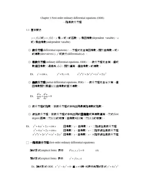
Chapter 1 First-order ordinary differential equations (ODE)一階常微分方程1.1 基本概念()x f y =或()t f y =，y 是x 或t 的函數，y 是因變數(dependent variable )，x 或t 是自變數(independent variable )◎ 微分方程(differential equations)：一方程式包含有因變數y 關於自變數x 或t的導數(derivatives)y y ′ ,&或微分(differentials)dy 。

◎ 常微分方程(ordinary differential equations, ODE)：一微分方程包含有一個或數個因變數（通常為()x y ）關於僅有一個自變數x 的導數。

Ex. 222)2(2 ,09 ,cos y x y e y y x y y x y x +=′′+′′′′=+′′=′◎ 偏微分方程(partial differential equations, PDE)：一微分方程包含至少有一個因變數關於兩個以上自變數的部分導數。

Ex. 02222=∂∂+∂∂yux u◎ 微分方程的階數：在微分方程式中所出現最高階導數的階數。

◎ 線性微分方程：在微分方程式中所出現的因變數因變數因變數或其導數僅有一次式(first degree)而無二次以上的乘積（自變數可以有二次以上的乘積）。

Ex. x y y x y cos 24=+′+′′ 因變數：y ，自變數：x ，二階線性常微分方程 x y y y y cos 24=+′+′′ 因變數：y ，自變數：x ，二階非線性常微分方程 222)2(2 y x y e y y x x +=′′+′′′′ 因變數：y ，自變數：x ，三階非線性常微分方程□ 一階常微分方程(first-order ordinary differential equations)隱式形式(implicit form) 表示 0),,(=′y y x F (4)顯式形式(explicit form) 表示 ),(y x f y =′Ex. 隱式形式ODE 0423=−′−y y x ，當0≠x 時，可表示為顯式形式234y x y =′□ 解的概念(concept of solution)在某些開放間隔區間b x a <<，一函數)(x h y =是常微分方程常微分方程0),,(=′y y x F 的解，其函數)(x h 在此區間b x a <<是明確(defined)且可微分的(differentiable)，其)(x h 的曲線（或圖形）是被稱為解答曲線(solution curve)。

数学专业英语－First Order Differential EquationsA differential equation is an equation between specified derivatives of a functio n, itsvalves,and known quantities.Many laws of physics are most simply and naturall y formu-lated as differential equations (or DE’s, as we shall write for short).For this r eason,DE’shave been studies by the greatest mathematicians and mathematical physicists si nce thetime of Newton..Ordinary differential equations are DE’s whose unknowns are functions of a s ingle va-riable;they arise most commonly in the study of dynamic systems and electric networks.They are much easier to treat than partial differential equations,whose unknown functionsdepend on two or more independent variables.Ordinary DE’s are classified according to their order. The order of a DE is d efined asthe largest positive integer, n, for which an n-th derivative occurs in the equati on. Thischapter will be restricted to real first order DE’s of the formΦ(x, y, y′)=0 (1)Given the function Φof three real variables, the problem is to determine all re al functions y=f(x) which satisfy the DE, that is ,all solutions of(1)in the follo wing sense.DEFINITION A solution of (1)is a differentiable function f(x) such thatΦ(x. f(x),f′(x))=0 for all x in the interval where f(x) is defined.EXAMPLE 1. In the first-other DEthe function Φis a polynomial function Φ(x, y, z)=x+ yz of three variables i n-volved. The solutions of (2) can be found by considering the identityd(x²+y²)/d x=2(x+yyˊ).From this identity,one sees that x²+y²is a con-stant if y=f(x) is any solution of (2).The equation x²+y²=c defines y implicitly as a two-valued function of x,for any positive constant c.Solving for y,we get two solutions,the(single-valued) functions y=±(c-x²)0.5,for each positive constant c.The graphs of these so-lutions,the so-called solution curves,form two families of scmicircles,which fill t he upper half-plane y>0 and the lower half-plane y>0,respectively.On the x-axis,where y=0,the DE(2) implies that x=0.Hence the DE has no solu tionswhich cross the x-axis,except possibly at the origin.This fact is easily overlook ed,because the solution curves appear to cross the x-axis;hence yˊdoes not exist, and the DE (2) is not satisfied there.The preceding difficulty also arises if one tries to solve the DE(2)for yˊ. Div iding through by y,one gets yˊ=-x/y,an equation which cannot be satisfied if y=0.The preceding difficulty is thus avoided if one restricts attention to regions where the DE(1) is normal,in the following sense.DEFINITION. A normal first-order DE is one of the formyˊ=F(x,y) (3)In the normal form yˊ=-x/y of the DE (2),the function F(x,y) is continuous i n the upper half-plane y>0 and in the lower half-plane where y<0;it is undefin ed on the x-axis.Fundamental Theorem of the Calculus.The most familiar class of differential equations consists of the first-order DE’s of the formSuch DE’s are normal and their solutions are descried by the fundamental tho rem of the calculus,which reads as follows.FUNDAMENTAL THEOREM OF THE CALCULUS. Let the function g(x)i n DE(4) be continuous in the interval a<x<b.Given a number c,there is one an d only one solution f(x) of the DE(4) in the interval such that f(a)=c. This sol ution is given by the definite integralf(x)=c+∫a x g(t)dt , c=f(a) (5)This basic result serves as a model of rigorous formulation in several respects. First,it specifies the region under consideration,as a vertical strip a<x<b in the xy-plane.Second,it describes in precise terms the class of functions g(x) consid ered.And third, it asserts the existence and uniqueness of a solution,given the “initial condition”f(a)=c.We recall that the definite integral∫a x g(t)dt=lim(maxΔt k->0)Σg(t k)Δt k , Δt k=t k-t k-1 (5ˊ)is defined for each fixed x as a limit of Ricmann sums; it is not necessary to find a formal expression for the indefinite integral ∫g(x) dx to give meanin g to the definite integral ∫a x g(t)dt,provided only that g(t) is continuous.Such f unctions as the error function crf x =(2/(π)0.5)∫0x e-t²dt and the sine integral f unction SI(x)=∫x∞[(sin t )/t]dt are indeed commonly defined as definite int egrals.Solutions and IntegralsAccording to the definition given above a solution of a DE is always a functi on. For example, the solutions of the DE x+yyˊ=0 in Example I are the func tions y=±(c-x²)0.5,whose graphs are semicircles of arbitrary diameter,centered at the origin.The graph of the solution curves are ,however,more easily describ ed by the equation x²+y²=c,describing a family of circles centered at the origi n.In what sense can such a family of curves be considered as a solution of th e DE ?To answer this question,we require a new notion.DEFINITION. An integral of DE(1)is a function of two variables,u(x,y),whic h assumes a constant value whenever the variable y is replaced by a solution y=f(x) of the DE.In the above example, the function u(x,y)=x²+y²is an integral of the DE x +yyˊ=0,because,upon replacing the variable y by any function ±( c-x²)0.5,we obtain u(x,y)=c.The second-order DEd²x/dt²=-x (2ˊ)becomes a first-order DE equivalent to (2) after setting dx/dx=y:y ( dy/dx )=-x (2)As we have seen, the curves u(x,y)=x²+y²=c are integrals of this DE.When th e DE (2ˊ)is interpreted as equation of motion under Newton’s second law,the integrals c=x²+y²represent curves of constant energy c.This illustrates an important prin ciple:an integral of a DE representing some kind of motion is a quantity that r emains unchanged through the motion.Vocabularydifferential equation 微分方程 error function 误差函数ordinary differential equation 常微分方程 sine integral function 正弦积分函数order 阶,序 diameter 直径derivative 导数 curve 曲线known quantities 已知量replace 替代unknown 未知量substitute 代入single variable 单变量strip 带形dynamic system 动力系统 exact differential 恰当微分electric network 电子网络line integral 线积分partial differential equation 偏微分方程path of integral 积分路径classify 分类 endpoints 端点polynomial 多项式 general solution 通解several variables 多变量parameter 参数family 族rigorous 严格的semicircle 半圆 existence 存在性half-plane 半平面 initial condition 初始条件region 区域uniqueness 唯一性normal 正规,正常Riemann sum 犁曼加identity 恒等(式)Notes1. The order of a DE is defined as the largest positive integral n,for which an nth derivative occurs i n the question.这是另一种定义句型,请参看附录IV.此外要注意nth derivative 之前用an 不用a .2. This chapter will be restricted to real first order differential equations of the formΦ(x,y,yˊ)=0意思是;文章限于讨论形如Φ(x,y,yˊ)=0的实一阶微分方程.有时可以用of the type代替of the form 的用法.The equation can be rewritten in the form yˊ=F(x,y).3. Dividing through by y,one gets yˊ=-x/y,…划线短语意思是:全式除以y4. As we have seen, the curves u(x,y)=x²+y²=c are integrals of this DE这里x²+y²=c 因c是参数,故此方程代表一族曲线,由此”曲线”这一词要用复数curves.5. Their solutions are described by the fundamental theorem of the calculus,which reads as follows.意思是:它们的解由微积分基本定理所描述,(基本定理)可写出如下.句中reads as follows 就是”写成(读成)下面的样子”的意思.注意follows一词中的”s”不能省略.ExerciseⅠ.Translate the following passages into Chinese:1.A differential M(x,y) dx +N(x,y) dy ,where M, N are real functions of two variables x and y, is called exact in a domain D when the line integral ∫c M(x,y) dx +N(x,y) dy is the same for all paths of int egration c in D, which have the same endpoints.Mdx+Ndy is exact if and only if there exists a continuously differentiable function u(x,y) such that M= u/ x, N=u/ y.2. For any normal first order DE yˊ=F(x,y) and any initial x0 , the initial valve problem consists of finding the solution or solutions of the DE ,for x>x0 which assumes a given initial valve f(x0)=c.3. To show that the initial valve problem is well-set requires proving theorems of existence (there isa solution), uniqueness (there is only one solution) and continuity (the solution depends continuously on t he initial value).Ⅱ. Translate the following sentences into English:1) 因为y=ч(x) 是微分方程dy/ dx=f(x,y)的解,故有dч(x)/dx=f (x,ч(x))2) 两边从x0到x取定积分得ч(x)-ч(x0)=∫x0x f(x,ч(x)) dx x0<x<x0+h3) 把y0=ч(x0)代入上式, 即有ч(x)=y0+∫x0x f(x,ч(x)) dx x0<x<x0+h4) 因此y=ч(x) 是积分方程y=y0+∫x0x f (x,y) dx定义于x0<x<x0+h 的连续解.Ⅲ. Translate the following sentences into English:1) 现在讨论型如 y=f (x,yˊ) 的微分方程的解,这里假设函数f (x, dy/dx) 有连续的偏导数.2) 引入参数dy/dx=p, 则已给方程变为y=f (x,p).3) 在y=f (x,p) x p=dy/dx p= f/ x+f/ p dp/dx4) 这是一个关于x和p的一阶微分方程,它的解法我们已经知道.5) 若(A)的通解的形式为p=ч(x,c) ,则原方程的通解为y=f (x,ч(x,c)).6) 若(A) 有型如x=ψ(x,c)的通解,则原方程有参数形式的通解 x=ψ(p,c)y=f(ψ(p,c)p)其中p是参数,c是任意常数.。

"
证明: 对y sinx,由于
y y sin x sin x 0
"
y cosx,y sin x 故对x (, ), 有
' "
故y sinx是微分方程 y" y 0在(,)上的一个解 . 同理y cosx是微分方程 y" y 0在(,)上的一个解 .
与其他学科的关系
• 常微分方程的形成与发展是和力学、天文学、物 理学，以及其他科学技术的发展密切相关的 • 数学的其他分支的新发展，如复变函数、李群、 组合拓扑学等，都对常微分方程的发展产生了深 刻的影响 • 当前计算机的发展更是为常微分方程的应用及理 论研究提供了非常有力的工具
1.1 常微分方程模型
SI模型 易感染者：Susceptible 已感染者：Infective
SIS模型
• 对无免疫性的传染病，假设病人治愈后会再次被 感染，设单位时间治愈率为mu
SIR模型（R：移出者（Removed））
• 对有很强免疫性的传染病，假设病人治愈后不会在 被感染，设在时刻t的愈后免疫人数为r(t)，称为移出 者，而治愈率l为常数
如
dy (2) xdy ydx 0 ; (1) 2 x; dx 3 2 d x dx (3) tx x 0; 2 dt dt
d 4x d 2x (4) 5 2 3x sin t; 4 dt dt
都是常微分方程
偏微分方程
如果在一个微分方程中,自变量的个数为两个或两 个以上,称为偏微分方程，PDE 如
n阶线性微分方程的一般形式
d y d y a1 ( x) n1 an ( x) y f ( x) n dx dx

高阶常系数齐次线性微分方程的解法凯歌【摘要】常微分方程是微积分学的重要组成部分，求解高阶微分方程是常微分方程的一难点问题，通常用适当的变量代换，达到降阶的目的来解决问题。

结合多年的教学经验，归纳总结给出高阶常系数齐次线性微分方程的一些求解方法，包括常系数齐次线性微分方程和欧拉方程以及可降阶的高阶微分方程等，并通过例题阐述各种方法。

%Ordinary Differential equation is an important part of differential and integration. Solving Ordinary Differential equation of difficult prob-lem is the differential equations of high order. Generally, in order to achieve the purpose to solve problems, it uses an appropriate variable substitution. With many years of teaching experience, summarizes to give some methods for solving the linear differential equation of higher-order, including homogeneous linear differential equation with constant coefficient, Euler equations and higher-order differential of reduce order and so on, gives an example to explain a variety of methods.【期刊名称】《现代计算机（专业版）》【年(卷),期】2016(000)002【总页数】4页(P26-28,51)【关键词】微分方程;特征方程;欧拉方程;齐次方程【作者】凯歌【作者单位】内蒙古财经大学统计与数学学院，呼和浩特 010070【正文语种】中文求解常微分方程的问题，常常通过变量分离、两边积分，如果是高阶微分方程则通过适当的变量代换，达到降阶的目的来解决问题。

genral solution of (4).
• Theorem. Let M(x,y) and N(x,y) be continuous and have continuous partial derivatives with respect x and y in the rectangle R consisting of those points (x,y) with a<x<b and c<y<d. There exists a function Q(x,y) such that
• Then, the initial-value problem
• dy/dx=f(x,y), y(x0)= y0
(6)
• has a unique solution y(x) on the interval
x0=< x <= x0 + α. In other words, if y(x) and z(x) are two solutions of (6), the y(x)
these functions is a constant multiple of the
other on I. The functions y1(x) and y2(x) are said to be linear independent on an interval I if there
are not linear dependent on I.
Review of terms for classifying firstorder ODEs.
• Although this really means F(x, y, dy/dx) = 0 for some F of 3 variables, all further adjectives assume the equation has the form dy/dx = f(x,y) for some real-valued f defined on a subset of R^2.

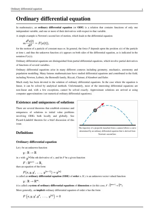
Ordinary differential equationIn mathematics, an ordinary differential equation (or ODE ) is a relation that contains functions of only one independent variable, and one or more of their derivatives with respect to that variable.A simple example is Newton's second law of motion, which leads to the differential equationfor the motion of a particle of constant mass m . In general, the force F depends upon the position x(t) of the particle at time t , and thus the unknown function x(t) appears on both sides of the differential equation, as is indicated in the notation F (x (t )).Ordinary differential equations are distinguished from partial differential equations, which involve partial derivatives of functions of several variables.Ordinary differential equations arise in many different contexts including geometry, mechanics, astronomy and population modelling. Many famous mathematicians have studied differential equations and contributed to the field,including Newton, Leibniz, the Bernoulli family, Riccati, Clairaut, d'Alembert and Euler.Much study has been devoted to the solution of ordinary differential equations. In the case where the equation is linear, it can be solved by analytical methods. Unfortunately, most of the interesting differential equations are non-linear and, with a few exceptions, cannot be solved exactly. Approximate solutions are arrived at using computer approximations (see numerical ordinary differential equations).The trajectory of a projectile launched from a cannon follows a curve determined by an ordinary differential equation that is derived fromNewton's second law.Existence and uniqueness of solutionsThere are several theorems that establish existence anduniqueness of solutions to initial value problemsinvolving ODEs both locally and globally. SeePicard –Lindelöf theorem for a brief discussion of thisissue.DefinitionsOrdinary differential equationLet ybe an unknown function in x with the n th derivative of y , and let Fbe a given functionthen an equation of the formis called an ordinary differential equation (ODE) of order n . If y is an unknown vector valued function,it is called a system of ordinary differential equations of dimension m (in this case, F : ℝmn +1→ ℝm ).More generally, an implicit ordinary differential equation of order nhas the formwhere F : ℝn+2→ ℝ depends on y(n). To distinguish the above case from this one, an equation of the formis called an explicit differential equation.A differential equation not depending on x is called autonomous.A differential equation is said to be linear if F can be written as a linear combination of the derivatives of y together with a constant term, all possibly depending on x:(x) and r(x) continuous functions in x. The function r(x) is called the source term; if r(x)=0 then the linear with aidifferential equation is called homogeneous, otherwise it is called non-homogeneous or inhomogeneous. SolutionsGiven a differential equationa function u: I⊂ R→ R is called the solution or integral curve for F, if u is n-times differentiable on I, andGiven two solutions u: J⊂ R→ R and v: I⊂ R→ R, u is called an extension of v if I⊂ J andA solution which has no extension is called a global solution.A general solution of an n-th order equation is a solution containing n arbitrary variables, corresponding to n constants of integration. A particular solution is derived from the general solution by setting the constants to particular values, often chosen to fulfill set 'initial conditions or boundary conditions'. A singular solution is a solution that can't be derived from the general solution.Reduction to a first order systemAny differential equation of order n can be written as a system of n first-order differential equations. Given an explicit ordinary differential equation of order n (and dimension 1),define a new family of unknown functionsfor i from 1 to n.The original differential equation can be rewritten as the system of differential equations with order 1 and dimension n given bywhich can be written concisely in vector notation aswithandLinear ordinary differential equationsA well understood particular class of differential equations is linear differential equations. We can always reduce an explicit linear differential equation of any order to a system of differential equation of order 1which we can write concisely using matrix and vector notation aswithHomogeneous equationsThe set of solutions for a system of homogeneous linear differential equations of order 1 and dimension nforms an n-dimensional vector space. Given a basis for this vector space , which is called a fundamental system, every solution can be written asThe n × n matrixis called fundamental matrix. In general there is no method to explicitly construct a fundamental system, but if one solution is known d'Alembert reduction can be used to reduce the dimension of the differential equation by one.Nonhomogeneous equationsThe set of solutions for a system of inhomogeneous linear differential equations of order 1 and dimension ncan be constructed by finding the fundamental system to the corresponding homogeneous equation and one particular solution to the inhomogeneous equation. Every solution to nonhomogeneous equation can then be written asA particular solution to the nonhomogeneous equation can be found by the method of undetermined coefficients or the method of variation of parameters.Concerning second order linear ordinary differential equations, it is well known thatSo, if is a solution of: , then such that:So, if is a solution of: ; then a particular solution of , isgiven by:. [1]Fundamental systems for homogeneous equations with constant coefficientsIf a system of homogeneous linear differential equations has constant coefficientsthen we can explicitly construct a fundamental system. The fundamental system can be written as a matrix differential equationwith solution as a matrix exponentialwhich is a fundamental matrix for the original differential equation. To explicitly calculate this expression we first transform A into Jordan normal formand then evaluate the Jordan blocksof J separately asTheories of ODEsSingular solutionsThe theory of singular solutions of ordinary and partial differential equations was a subject of research from the time of Leibniz, but only since the middle of the nineteenth century did it receive special attention. A valuable but little-known work on the subject is that of Houtain (1854). Darboux (starting in 1873) was a leader in the theory, and in the geometric interpretation of these solutions he opened a field which was worked by various writers, notably Casorati and Cayley. To the latter is due (1872) the theory of singular solutions of differential equations of the first order as accepted circa 1900.Reduction to quadraturesThe primitive attempt in dealing with differential equations had in view a reduction to quadratures. As it had been the hope of eighteenth-century algebraists to find a method for solving the general equation of the th degree, so it was the hope of analysts to find a general method for integrating any differential equation. Gauss (1799) showed, however, that the differential equation meets its limitations very soon unless complex numbers are introduced. Hence analysts began to substitute the study of functions, thus opening a new and fertile field. Cauchy was the first to appreciate the importance of this view. Thereafter the real question was to be, not whether a solution is possible by means of known functions or their integrals, but whether a given differential equation suffices for the definition of a function of the independent variable or variables, and if so, what are the characteristic properties of this function.Fuchsian theoryTwo memoirs by Fuchs (Crelle, 1866, 1868), inspired a novel approach, subsequently elaborated by Thomé and Frobenius. Collet was a prominent contributor beginning in 1869, although his method for integrating a non-linear system was communicated to Bertrand in 1868. Clebsch (1873) attacked the theory along lines parallel to those followed in his theory of Abelian integrals. As the latter can be classified according to the properties of the fundamental curve which remains unchanged under a rational transformation, so Clebsch proposed to classify the transcendent functions defined by the differential equations according to the invariant properties of the corresponding surfaces f = 0 under rational one-to-one transformations.Lie's theoryFrom 1870 Sophus Lie's work put the theory of differential equations on a more satisfactory foundation. He showed that the integration theories of the older mathematicians can, by the introduction of what are now called Lie groups, be referred to a common source; and that ordinary differential equations which admit the same infinitesimal transformations present comparable difficulties of integration. He also emphasized the subject of transformations of contact.A general approach to solve DE's uses the symmetry property of differential equations, the continuous infinitesimal transformations of solutions to solutions (Lie theory). Continuous group theory, Lie algebras and differential geometry are used to understand the structure of linear and nonlinear (partial) differential equations for generating integrable equations, to find its Lax pairs, recursion operators, Bäcklund transform and finally finding exact analytic solutions to the DE.Symmetry methods have been recognized to study differential equations arising in mathematics, physics, engineering, and many other disciplines.Sturm–Liouville theorySturm–Liouville theory is a theory of eigenvalues and eigenfunctions of linear operators defined in terms of second-order homogeneous linear equations, and is useful in the analysis of certain partial differential equations.Software for ODE solving•FuncDesigner (free license: BSD, uses Automatic differentiation, also can be used online via Sage-server [2])•VisSim [3] - a visual language for differential equation solving•Mathematical Assistant on Web [4] online solving first order (linear and with separated variables) and second order linear differential equations (with constant coefficients), including intermediate steps in the solution.•DotNumerics: Ordinary Differential Equations for C# and [5] Initial-value problem for nonstiff and stiff ordinary differential equations (explicit Runge-Kutta, implicit Runge-Kutta, Gear’s BDF and Adams-Moulton).•Online experiments with JSXGraph [6]References[1]Polyanin, Andrei D.; Valentin F. Zaitsev (2003). Handbook of Exact Solutions for Ordinary Differential Equations, 2nd. Ed.. Chapman &Hall/CRC. ISBN 1-5848-8297-2.[2]/welcome[3][4]http://user.mendelu.cz/marik/maw/index.php?lang=en&form=ode[5]/NumericalLibraries/DifferentialEquations/[6]http://jsxgraph.uni-bayreuth.de/wiki/index.php/Differential_equationsBibliography• A. D. Polyanin and V. F. Zaitsev, Handbook of Exact Solutions for Ordinary Differential Equations (2nd edition)", Chapman & Hall/CRC Press, Boca Raton, 2003. ISBN 1-58488-297-2• A. D. Polyanin, V. F. Zaitsev, and A. Moussiaux, Handbook of First Order Partial Differential Equations, Taylor & Francis, London, 2002. ISBN 0-415-27267-X• D. Zwillinger, Handbook of Differential Equations (3rd edition), Academic Press, Boston, 1997.•Hartman, Philip, Ordinary Differential Equations, 2nd Ed., Society for Industrial & Applied Math, 2002. ISBN 0-89871-510-5.•W. Johnson, A Treatise on Ordinary and Partial Differential Equations (/cgi/b/bib/ bibperm?q1=abv5010.0001.001), John Wiley and Sons, 1913, in University of Michigan Historical Math Collection (/u/umhistmath/)• E.L. Ince, Ordinary Differential Equations, Dover Publications, 1958, ISBN 0486603490•Witold Hurewicz, Lectures on Ordinary Differential Equations, Dover Publications, ISBN 0-486-49510-8•Ibragimov, Nail H (1993), CRC Handbook of Lie Group Analysis of Differential Equations Vol. 1-3, Providence: CRC-Press, ISBN 0849344883.External links•Differential Equations (/Science/Math/Differential_Equations//) at the Open Directory Project (includes a list of software for solving differential equations).•EqWorld: The World of Mathematical Equations (http://eqworld.ipmnet.ru/index.htm), containing a list of ordinary differential equations with their solutions.•Online Notes / Differential Equations (/classes/de/de.aspx) by Paul Dawkins, Lamar University.•Differential Equations (/diffeq/diffeq.html), S.O.S. Mathematics.• A primer on analytical solution of differential equations (/mws/gen/ 08ode/mws_gen_ode_bck_primer.pdf) from the Holistic Numerical Methods Institute, University of South Florida.•Ordinary Differential Equations and Dynamical Systems (http://www.mat.univie.ac.at/~gerald/ftp/book-ode/ ) lecture notes by Gerald Teschl.•Notes on Diffy Qs: Differential Equations for Engineers (/diffyqs/) An introductory textbook on differential equations by Jiri Lebl of UIUC.Article Sources and Contributors7Article Sources and ContributorsOrdinary differential equation Source: /w/index.php?oldid=433160713 Contributors: 48v, A. di M., Absurdburger, AdamSmithee, After Midnight, Ahadley,Ahoerstemeier,AlfyAlf,Alll,AndreiPolyanin,Anetode,Ap,Arthena,ArthurRubin,BL,BMF81,********************,Bemoeial,BenFrantzDale,Benjamin.friedrich,BereanHunter,Bernhard Bauer, Beve, Bloodshedder, Bo Jacoby, Bogdangiusca, Bryan Derksen, Charles Matthews, Chilti, Chris in denmark, ChrisUK, Christian List, Cloudmichael, Cmdrjameson, Cmprince, Conversion script, Cpuwhiz11, Cutler, Delaszk, Dicklyon, DiegoPG, Dmitrey, Dmr2, DominiqueNC, Dominus, Donludwig, Doradus, Dysprosia, Ed Poor, Ekotkie, Emperorbma, Enochlau, Fintor, Fruge, Fzix info, Gauge, Gene s, Gerbrant, Giftlite, Gombang, HappyCamper, Heuwitt, Hongsichuan, Ht686rg90, Icairns, Isilanes, Iulianu, Jack in the box, Jak86, Jao, JeLuF, Jitse Niesen, Jni, JoanneB, John C PI, Jokes Free4Me, JonMcLoone, Josevellezcaldas, Juansempere, Kawautar, Kdmckale, Krakhan, Kwantus, L-H, LachlanA, Lethe, Linas, Lingwitt, Liquider, Lupo, MarkGallagher,MathMartin, Matusz, Melikamp, Michael Hardy, Mikez, Moskvax, MrOllie, Msh210, Mtness, Niteowlneils, Oleg Alexandrov, Patrick, Paul August, Paul Matthews, PaulTanenbaum, Pdenapo, PenguiN42, Phil Bastian, PizzaMargherita, Pm215, Poor Yorick, Pt, Rasterfahrer, Raven in Orbit, Recentchanges, RedWolf, Rich Farmbrough, Rl, RobHar, Rogper, Romanm, Rpm, Ruakh, Salix alba, Sbyrnes321, Sekky, Shandris, Shirt58, SilverSurfer314, Ssd, Starlight37, Stevertigo, Stw, Susvolans, Sverdrup, Tarquin, Tbsmith, Technopilgrim, Telso, Template namespace initialisation script, The Anome, Tobias Hoevekamp, TomyDuby, TotientDragooned, Tristanreid, Twin Bird, Tyagi, Ulner, Vadimvadim, Waltpohl, Wclxlus, Whommighter, Wideofthemark, WriterHound, Xrchz, Yhkhoo, 今古庸龍, 176 anonymous editsImage Sources, Licenses and ContributorsImage:Parabolic trajectory.svg Source: /w/index.php?title=File:Parabolic_trajectory.svg License: Public Domain Contributors: Oleg AlexandrovLicenseCreative Commons Attribution-Share Alike 3.0 Unported/licenses/by-sa/3.0/。

一、线性微分方程解的结构 定理1：如果 y1 ( x), y2 ( x)是线性 齐次方程
y p( x) y q( x) y 0
的解，则 cy1 ( x) 和 y1 ( x) y2 ( x) 也是线性齐次方程的解。
线性相关：如果 y1 ( x) 与 y2 ( x)之比 为常数。
（1）先求出非齐次线性方程所对应的齐次方程的通 解 . （2）根据所求出的齐次方程的通解设出非齐次线性 方程的解(将所求出的齐次方程的通解中的任意常数 C 改 为待定函数 C(x)即可). （3）将所设解代入非齐次线性方程,解出 C(x),并写 出非齐次线性方程的通解.
例1
解
y x ln x 求方程 y 的通解. x
ቤተ መጻሕፍቲ ባይዱ
2. y f ( x, y) 型方程 (或F ( x, y, y) 0)
特点：方程中不显含未知函数 y. 解法 dp 为降阶，令 y p, 则 y ,
dx
原方程变为 p f ( x, p), 这是一个以 p 为
未知函数的一阶方程；
解上述一阶方程，得 y p ( x, C1 ), 再积分一次，得通解：
四、微分方程的几何意义
积分曲线：微分方程的特解
y f (x)
的几何图形，称为微分方程的
一条积分曲线。
§6.2
可分离变量的微分方程
dy f ( x) g ( y ) dx
1 dy f ( x)dx g ( y)
一、变量可分离的微分方程 行如：
解法：
两边积分有
1 dy f ( x)dx g ( y)
方程解法：通过 n 次积分 就可得到方程的通解.
例1
求方程 y

yn1 yn h ( xn , yn , h)
§6.1 概述
常微分方程数值解法所考虑的主要问 题有：
(1) 方法推导。即用什么样的途径来导出 递推格式； (2) 收敛性。即差分方程的解能否充分逼 近微分方程初值问题的解； (3) 误差传播。在递推过程中，每一步 都会产生截断误差和舍入误差，这个误 差是否对后续各步产生严重影响。
第六章 常微分方程的数值解法
§6.4 改进欧拉方法
(modified Euler’s method)
§6.4 改进欧拉方法
梯形方法比欧拉方法更精确，但是一 种隐式方法，求解方程计算量大。 实际计算中，迭代初始值yn+1可取欧拉 方程结果，迭代一次即可，这样的计算 公式叫改进欧拉法。
§6.4 改进欧拉方法
§6.1 概述 理论做了系统阐述。在代数数论领域，他引进了相 应的符号表示法及其计算法则，建立起被称为“李 普希兹代数”的超复数系。在微分几何方面，他自 1869年起对黎曼关于n维流形的度量结构的工作做 出进一步阐述和推广，开创了微分不变量理论的研 究，因此被认为是协变微分的奠基人之一。他的工 作后来被里奇有效地用于张量分析。
§6.1 概述
本章我们将学习一阶常微分方程的初 值问题的数值解：
dy f ( x, y ) dx y ( x0 ) y0 (1) (2)
一般情况下，方程(1)有无穷多个解， 式(2)是确定解的初始条件。
§6.1 概述
定义： 如果一元函数y(x)对一切 a x b 满足 (1) ( x, y( x)) 平面区域D
计算方法 (力学系本科生)
第六章 常微分方程 的数值解法 (Integration of ordinary differential equations)

dy ky dt


dy ky dt
Rate of change is proportional to the amount present.
1 dy k dt Divide both sides by y. y 1 y dy k dt Integrate both sides.
Combined constants of integration
1 y 2 x C

Family of solutions (general solution) of a differential equation
Example
dy x dx y
ydy xdx
y2 x2 C
Initial conditions
• In many physical problems we need to find the particular solution that satisfies a condition of the form y(x0)=y0. This is called an initial condition, and the problem of finding a solution of the differential equation that satisfies the initial condition is called an initial-value problem. • Example (cont.): Find a solution to y2 = x2 + C satisfying the initial condition y(0) = 2. 22 = 0 2 + C C=4 y2 = x 2 + 4

4. Numerical Methods for solving Ordinary Differential EquationsWhenever a physical law involves a rate of change of a function, such as velocity, acceleration, etc., it will lead to a differential equation. For this reason differential equations occur frequently in physics and engineering.Analytical solutions can be found to differential equations, but are hard to derive for more complicated cases. Numerical solution methods are then suitable to apply when solving the problems. Solving engineering problems ultimately comes down to numerical results. The need for numerical methods for obtaining numerical results is obvious. Indeed, many engineering problems can be solved only approximately.Mechanical engineering is part of the product development process. Some aspects on this are pointed out here before introducing numerical methods of solving ordinary differential equations for initial value and boundary value problems. A hydrodynamic bearing problem is used as an application example. A brief introduction to engineering Tribology is therefore given prior to solving this problem.4.1. Introduction to ComputationThe fraction of “real world” problems that a design engineer will face during his/her professional life that is possible to solve by pure analytical methods is small compared to problems that need to be solved for numerically. However, good command of analytical methods is necessary for understanding most numerical methods and to make use of them in the best possible way. Using them side by side is very powerful in engineering analysis.Carelessly speaking, numerical methods is the science of guessing. Guessing is very easy. To be of any good the method must however also be:- Effective, that is: give a solution within reasonable time.- Stable, that is: errors must not accumulate in an uncontrolled way.- Accurate, that is: errors of the final solution must be negligible.Thus, more carefully speaking, numerical methods is the science of guessing intelligently.Physical problems are often described by differential equations. Numerical methods for differential equations are of great importance to the engineer because practical problems often lead to differential equations that cannot be solved by standard analytical methods.The development of numerical methods is strongly influenced and determined by the computer, which has become indispensable in the mathematical work of every engineer, and by the tremendous progress in digital computation. It is clear that the high speed, reliability and flexibility of the computer provide access to practical problems that in precomputer times were not within the reach of numerical work. For instance, the solution of very large systems of linear equations is of that type. The study of error has become important in both the development of new numerical methods and in applying them to problems.The solution of a problem involving numerical work consists of the following steps.1.Modelling. Translating a given physical or other information and data into a mathematical model, that is, formulating the problem in mathematical terms, taking also into account the use of a computer.2.Algorithm. Choice of numerical methods, together with a preliminary error analysis (estimation of error, determination of steps size, etc.3.Programming. Usually this starts with a flowchart showing a block diagram of the procedures to be performed by the computer, and then writing a program.4.Operation.5.Interpretation of the results. Understanding the meaning and the implications of the mathematical solution for the original problem in terms of physics- or wherever the problem comes from. This may also include the decision to rerun if further results are needed.It should be pointed out that the computer does not relieve the user of planning the work carefully; on the contrary , the computer demands much more careful planning. Also, the computer does not reduce the need for detailed understanding of the problem area or of the related mathematics.Since in computations we work with a finite number of digits and carry out finitely many steps, the methods of numerical analysis are finite processes, and a numerical result is an approximate value of the (unknown) exact result. The difference between the exact value and the approximated value is called the error.Depending on the source of error, we may distinguish between experimental errors, truncation errors, round-off errors and programming errors (blunders). Experimental errors are errors of given data (probably arising from measurements). Truncation errors are the errors caused by prematurely breaking off a sequence of computational steps necessary for producing an exact result. These errors depend on the computational method used and must be dealt with individually for each method. Round-off errors are arising from the process of rounding off during computation.Rounding errors may ruin a computation completely. In general, they are the more dangerous the more arithmetic operations we have to perform. It is therefore important to analyse computational programs for rounding off errors to be expected and to find an arrangement of the computations such that the effect of rounding errors is as small as possible. A sequence of computations by well-defined rules is called an algorithm , and an algorithm is called stable if errors in intermediate results have little influence on the final results. If, however, intermediate results have a very strong effect on the final result, the algorithm is called unstable . This numerical instability should be carefully distinguished from mathematical instability of a given problem; the problem is then called ill-conditioned .Many program packages are available for computing results. However, the use of standard programs still requires knowledge of the purpose of the program and its limitations. Furthermore, we should be aware that most problems cannot be solved simply by applying some standard program, but we must often devise new numerical methods by adapting standard methods to a new task.4.2. Ordinary Differential EquationsRoughly, differential equations are equations that contain derivatives of an unknown function. Differential equations arise in many engineering and other applications, as mathematical models of various physical and other systems.An ordinary differential equation (ODE) is an equation that involves one or several derivatives of an unspecified function y of only one variable x . The equation may also involve y itself, given functions of x , and constants. For example()222233222y x dx y d e dx dy dx y d x x +=+ (4.1)is an ordinary differential equation.The word ordinary distinguishes such an equation from a partial differential equation , which involves partial derivatives of an unspecified function of two or more independent variables. For example02222=∂∂+∂∂yu x u (4.2)is a partial differential equation. Only ordinary differential equations are considered here.A differential equation is said to be of order n if the n th derivative of y with respect to x is the highest derivative in the equation. Equation (4.2) is of the third order.A complete differential equation problem always involves both the equation and some boundary or initial value(s).4.3. Initial value problemsAn initial value problem consists of a differential equation and a condition the solution must satisfy (or several conditions referring to the same value of x if the equation is of higher order). Here, initial value problems of the formdy dxf x y=(,), y x y()00= (4.3)are considered, assuming f to be such that the problem has a unique solution on some interval containing x0.As an example of an initial value problem we will study the equation of motion for a body (particle).Example 4.1After burnout a toy rocket has a velocity of 60 m/s and is subjected only to gravitation and air resistance. The air resistance is a function of the speed of the rocket according to R kv=2, where k is a constant including the density of the air, the cross-sectional area of the rocket and the coefficient of drag. Determine the velocity as a function of time.Newton’s second law givesdv dt g k m v =−−2, v ()060= m/sThis is a differential equation of the type shown in equation (4.3).The solution isv t k mgv k mg g k mg t ()tan arctan =⎛⎝⎜⎞⎠⎟−⎛⎝⎜⎞⎠⎟⎛⎝⎜⎞⎠⎟10, 0≥vAlthough the differential equation of example 4.1 was easily solved analytically, we will try to solve it numerically as well. The purpose is to introduce some numerical methods that can be used to solve similar equations that are not possible to solve analytically.Physical problems are not always that easy that a single first order differential equation is enough. Often a system of differential equations arises, even for many rather simple problems. It is, however, easy to generalise the methods discussed to solve also systems of equations.4.3.1. The Euler MethodLooking at equation (4.3), the most obvious procedure would be to use the explicitly provided information of the slope of the function. Knowing the initial value y x y ()00=, then y 1, that is, the value of y at x x h 10=+ would bey y x h y x dy dxx y h y f x y h 10000000=+=+⋅=+⋅()()(,)(,) (4.4)which is a Taylor series expansion of y , including the first two terms only.Repeating this for x x h 202=+ givesy y x h y x dy dx x y h y f x y h 201111112=+=+⋅=+⋅()()(,)(,) (4.5)Generally the method can be described byy y f x y h n n n n +=+⋅1(,), n = 0, 1, 2,... (4.6)This is Euler’s method and it is called a one-step explicit method. A graphical interpretation is shown in figure 4-1. The (only) advantage of this method is its simplicity. The disadvantages concern instability and accuracy.Figure 4-1. Graphical interpretation of The Euler Method.The method is only conditionally stable. Special conditions for the coefficients must be fulfilled, and even then, the method often requires a very small step h in order to give satisfactory accuracy.Since the next term in the Taylor series would involve h2, the local truncation error is of that order of magnitude, often denoted O(h2). The total truncation error at the end of a finite interval is of O(h).This means that doubling the number of steps, for a given interval of x, would approximately decrease the total truncation error by one half, which is not so good. Especially if the interval of interest is rather large, the method would require too much of computer time, that is, being ineffective.Also bearing in mind that a higher number of steps increase the sum of round-off errors, present in all computation, the method is not very attractive, except for introducing some general aspects of numerical methods and for some simple problems. Knowing the Euler method is a good start when learning more sophisticated methods that are more accurate and computationally efficient.For a deeper discussion on stability and truncation errors, see for example (Akai, 1994), (Buchanan and Turner, 1992) or (Lindfield and Penny, 2000).With this knowledge we now return to example 4.1. Below is a Matlab-code for the Euler Method and figure 4-2 shows solutions of the problem for different values of the step h. In the same diagram the exact solution is shown for comparison. The curves are physically correct only for v≥ 0.Main script% Program ROCKET_41% Solves the rocket equation from example 4.1 using Euler's method% with various numbers of steps. The studied interval of 3 seconds% is divided into 8 steps (x), 16 steps (+) and 32 steps (o).% The exact solution is shown in the same graph for comparison.global g k m v0 % constants and initial valueg=9.81; k=0.004; m=0.1; v0=60;[t,v]=fplot('exact41',[0,3]);plot(t,v,'k'); xlabel('time (s)'); ylabel('velocity (m/s)');axis([0 3 -10 v0]); grid on; hold on; % exact solution[t,v]=euler1('rockeq1',0,3,v0,8);plot(t,v,'kx'); hold on; % eight steps[t,v]=euler1('rockeq1',0,3,v0,16);plot(t,v,'k+'); hold on; % sixteen steps[t,v]=euler1('rockeq1',0,3,v0,32);plot(t,v,'ko'); hold on; % thirtytwo stepsFunctions (in separate script files)function v=exact41(t)global g k m v0 % constants and initial valuer=sqrt(k/m/g);v=tan(atan(v0*r)-g*r*t)/r;function [x,y]=euler1(f,x0,xf,y0,nstep)h=(xf-x0)/nstep;x=x0; y=y0; xn=x0; yn=y0;for i=2:nstep+1xn1=xn+h; yn1=yn+feval(f,xn,yn)*h; % calculate new valuesx=[x,xn1]; y=[y,yn1]; % collect values for output xn=xn1; yn=yn1; % next input values end;function vprime=rockeq1(t,v)global g k mvprime=-g-k/m*v^2;Figure 4-2. The Euler Method for example 4.1.4.3.2. Richardson ExtrapolationCalculation of the f-values is usually the most time consuming part of solving a differential equation numerically. The number of necessary f-calculations should therefore be as low as possible. For good accuracy the Euler method discussed requires many steps and thus many f-calculations.A beautiful way of overcoming this problem is to combine the previous method with (repeated) Richardson Extrapolation. In this way it is often possible to decrease the number of f-calculations to a tiny fraction of what would have been needed with the original method.The genius idea of Richardson Extrapolation is to use the knowledge we have about the truncation error. An example is used for illustration.Example 4.2 Determine, by Euler’s method combined with Richardson Extrapolation, the value of y at x = 0,08 if the differential equation isdy dx y x =−+ , y ()01=The analytical solution isy e x x =+−−21giving y (0,08) = 0,926232692... as will be used for comparison.Now solving it with Euler’s method gives y (0,08) = 0,92000000 using only one step, and y (0,08) = 0,92320000 using two steps. None of the values have more than two correct decimals.However, for Euler’s method we know that the total truncation error is of the typeT c h c h c h =+++12233Kwhere c i are “constants”. Having calculated y (0,08) for two different step-lengths we now try to eliminate the first term in the truncation error. Index c is used for “correct/corrected”. y y c h y y c h h c h c ≈+≈+⎧⎨⎪⎩⎪1212Multiplying the second equation by two and subtracting the first gives22y y y h h c −≈which can be written asy y y y c h h h ≈+−=+−=22092320000092320000092000000092640000(),(,,),The error of y c would now be expected to be of O(h 2).Encouraged by the improvement we calculate the value of y (0,08) = 0,92473632, using foursteps, and repeats the procedure above, now involving this latter value and the two-step valuewe already have.y y y y c h h h ≈+−=+−=22092473632092473632092320000092627264(),(,,),The truncation errors of the y c -values we have calculated so far is of the typeT c h c h c h =++223344Kand it is now possible to eliminate the second term between these two latter values. That is()()(y y c h y y c h c h cc c h cc ≈+≈+⎧⎨⎪⎩⎪222222Multiplying the second equation by four and subtracting the first gives432()()y y y c h c h cc −≈which can be written as y y y y cc c h c h c h ≈+−=+−=()(()()),(,,),2230926272640926272640926400003092623019The error of y cc would now be expected to be of O(h 3).Adding Euler-values for eight steps and systematically repeating the procedure gives thescheme below and the value of y(0,08) = 0,92623271, see table 3.1.Table 3.1. Richardson Extrapolation Scheme.h y (0,08) Denominator 1 Denominator 3 Denominator 70,08 0,920000000,040,92320000 + 0,00320000 = 0,92640000 0,020,92473632 + 0,00153632 = 0,92627264 - 0,00004245 = 0,92623019 0,01 0,92548939 + 0,00075307 = 0,92624246 - 0,00001006 = 0,92623240 +0,00000032 = 0,92623271As noticed, this value is correct to seven decimals.The total number of f -calculations is (1+2+4+8) = 15. To achieve the same accuracy by usingEuler’s method alone, approximately 500 000 f -calculations would have been needed. Thisclearly implies a considerable difference in computer time between the two methods.This is one of many examples that it is good to know something about numerical methods'theories when using computers for computational engineering (before screaming for a morepowerful computer).In fact, it supports the general truth that “There is nothing more useful in practice than a goodtheory”.The Richardson Extrapolation Procedure can generally be described as follows.If the truncation error is of the typeK 321321p p p h c h c h c T ++=and if we have the two approximations y h and y qh (q > 1), an improved value of y is11−−+=p qh h h c q y y y yThe truncation error of c y is then of the order of magnitude of 22p h c .By systematically repeating this procedure the truncation error terms can be successivelyeliminated. Besides improved effectiveness the method also automatically gives an errorestimation. For a further discussion on the Richardson Extrapolation Procedure, see forexample (Akai, 1994) or (Buchanan and Turner, 1992).4.4. Boundary value problemsWhen conditions are at different values of the variable x , we have a boundary value problem .Many structural mechanics problems are of this kind. For example, for a beam on two rigidsupports we know that the deflection at each support is zero, and the deflection forintermediate points is described by a differential equation. The pressure build-up in slider padbearings is an other field of application that can be modelled as a boundary value problem andis dealt with in Engineering Tribology .Weighted residual methods are one type methods that can be applied to solve boundary value problems. A brief introduction to Engineering Tribology is given below before presenting and exemplifying the use of three specific weighted residual methods on a bearing problem.4.4.1 Introduction to Engineering TribologyTribology has been studied for a very long time. Most likely, in one way or the other, since man started to move things around, and of course, especially when we started to use machines of various types.The word Tribology originates from the Greek word Tribos, which means rubbing. However, Engineering Tribology embraces a lot more than just the study of rubbing. Tribology is the science and technology of interacting surfaces in relative motion and of related subjects and practices. This includes every aspect of friction, lubrication, and wear. For a more complete introduction and an excellent review of the subject, see (Williams, 1994).Although the use of sliding bearings has a long history it was not until the end of the nineteenth century that a theoretical explanation was given to why this type of bearing works. In his famous work from 1886, professor Osborne Reynolds derived a differential equation that governs the pressure build-up between two surfaces separated by a thin lubricating fluid film (Reynolds, 1886).This was the take-off for a tremendous development in the science of tribology, which also made it possible to improve bearing performance in practice. Again, “There is nothing more useful in practice than a good theory”.Professor Reynolds arrived at his equation by studying the full Navier-Stokes Equation. By making some genial assumptions and approximations, valid for most bearing applications, he was able to reduce this system of coupled partial differential equations into a single partial differential equation of two (three with time) variables.In this way it became possible, in spite of the lack of computers at that time, to theoretically determine the pressure distribution for some simple bearing configurations, and thereby explain why and how hydrodynamically lubricated bearings work.Cancelling terms in equations, by reasoning in orders of magnitude based on experience and feeling, is by the way very much what engineering science is about. Just deriving equations that are impossible (or costly) to solve can be done by any theorist.4.4.2 The One-Dimensional Reynolds’ EquationThe main steps in the derivation of the Reynolds’ equation based on the Reynolds’ assumptions are given here.Figure 4-3 shows schematically a sliding bearing. A thin film of lubricant, greatly exaggerated in the figure, separates the surfaces of the two solids. To get a pressure build-up in this film, as the lower solid moves, the gap between the solids must be convergent, at least at some part.UFigure 4-3. Slider bearing with one-dimensional flow.The following assumptions are now made:A1. Body forces (inertial and gravitational) are neglected, which means that surface forces must be in equilibrium.A2. The pressure and the viscosity are both considered to be constant through the thickness of the film.A3. Derivatives of velocity across the film thickness are far more important than any other velocity derivatives.A4. The flow is laminar.A5. The lubricant is considered to be Newtonian.A6. The lubricant adheres perfectly to the surfaces of the solids.Assumptions A1-A4 are due to the very thin film and assumptions A5-A6 are true for manycommonly used lubricants and bearing materials, although exceptions exist.For now we also make an additional assumption of one-dimensional flow, which will reduceReynolds’ equation further to an ordinary differential equation for the pressure distribution.Now, studying the infinitesimal fluid element of figure 4-4 and demanding equilibrium (A1)in the x -direction gives (b is the width of the element perpendicular to the plane of this paper)Figure 4-4. Infinitesimal fluid element.→: 02()2()2()2(=++−−+−−bdx dz z bdx dz z bdz dx dx dp p bdz dx dx dp p ∂∂ττ∂∂ττ dp dx z=∂τ∂ (4.7)For a Newtonian (A5) fluid in laminar flow (A4)τη∂∂∂∂=+()u z w x(4.8)where η is the viscosity of the fluid and u and w is the velocity in the x - and z -direction,respectively. Equation (4.8) is the fluid mechanics equivalent of Hooke's law for solids.Instead of shear distortion we now have shear distortion rate.The second term of equation (4.8) is cancelled due to (A3), which givesτη∂∂=u z(4.9)Combining equation (4.9) and equation (4.7) now gives∂∂η221u zdp dx = (4.10)since the viscosity is not a function of z (A2).Also due to (A2) and our assumption of one-dimensional flow, p is only a function of x , that is: dp dxis not a function of z , and equation (4.10) can be integrated directly.Doing this gives)()(21)(12121x C z x C z dx dp u x C z dxdp z u +⋅+⋅=+⋅=ηη∂∂where C 1(x ) and C 2(x ) are determined by using the following boundary conditions (A6)⎩⎨⎧==0),()0,(h x u U x uThis gives the velocity profile of the fluid flow in the bearing gap asu U z h dp dxzh z =−−−()()1122η (4.11)As can be seen, this velocity profile is made up of two components. The first is called thevelocity term, since it is due to the velocity of the bearing surface. This is a linear profile. Thesecond term is called the pressure term, since it is due to the pressure derivative. This is aparabolic profile. The sum of these profiles gives the actual velocity profile, see figure 4-5.+=Figure 4-5. Velocity profile of the fluid flow in the bearing gap.Now, since the velocity profile is known it is possible to determine the fluid flow according to∫∫−−−===)(02)(0))(21)1((x h x h dz z zh dxdp h z U b udz b qb Q η givingq Uh h dp dx=−2123η (4.12)Conservation of mass implies that the same amount of lubricant must pass any x -position, thatisd dxqb ()ρ=0This givesd dx h dp dx U d dxh ()()ρηρ36= (4.13)which is The One-Dimensional Reynolds’ Equation for steady-state operation .If the density and the viscosity of the lubricant are constant, we getd dxh dp dx U dh dx ()36=η (4.14)A liquid lubricant is (almost) incompressible, so in that case the assumption of constantdensity is very good.The assumption of constant viscosity is somewhat more questionable, since for a liquid lubricant viscosity is highly dependent on temperature.However, since bearings are usually designed for a low temperature rise of the lubricant, as it passes through the bearing and absorbs the power loss, the assumption is often not so bad.How Reynolds’ equation can be used for bearing calculations will be shown by an example.Example 4.3The figure shows a slider pad bearing having an exponential height-function according to h(x) = h0e-10x,h0 = 60 μm. The width of the bearing is 200 mm (perpendicular to the paper), the viscosity of the oil lubricant is 0,01 Ns/m2, and the velocity of the lower bearing surface is 10 m/s. The pressure at the front and end edges of the bearing is set to zero. The side edges of the bearing are sealed, giving a one-dimensional flow. Determine the load capacity F of the bearing.Reynolds’ equation givesd dxhdpdxh e h ex x (),()31010 600110106=⋅⋅⋅−⋅⋅=−−−which is integrated once tohdpdxh e Cx310106=+−,dp dx h e h e C h e h e C h e x x x x x=+=+−−−060601003103103103022010330,()(),and twice to p h e C h e C x x =++0620300220103302,C 1 and C 2 are now determined by the boundary conditionsp p ()(,)00010==⎧⎨⎩ =>0620300062030002103202210332,,h C h C h e C h e C ++=++=⎧⎨⎪⎪⎩⎪⎪ =>⎩⎨⎧⋅−=⋅−=−625110544,510808,1C C giving p e e x x =−−1083332790554462030(,,,)The load is now obtained by integrating pressure times area over the bearing surfaceF pbdx e e dx x x ==⋅−−=⋅∫∫01620300014021083332790554466610,,,(,,,),Thus, the answer is F = 67 kN.The shear stress at, for example, the lower bearing surface is easily derived. Combiningequation (4.9) and equation (4.11) and putting z = 0 givesτη∂∂η==−−uzU h h dp dx 2 (4.15)The frictional force is obtained by integrating this shear stress over the bearing surface. The power loss is obtained by multiplying this force by the velocity U .The relative power loss is defined as the power loss divided by the load capacity. Optimum design often aims at minimising the relative power loss.Although the differential equation was easily solved analytically, we will try to solve it numerically as well. The introduced numerical methods can be used to solve similar equations that are not possible to solve analytically.4.4.3. Weighted Residual MethodsWeighted residual methods can be applied to solve boundary value problems like the hydrodynamic bearing problem governed by Reynolds equation. Studying the concept of weighted residuals is also a good background for understanding the generalised finite element approach that is a powerful tool for solving various engineering problems. The general idea for this type of methods and three specific methods are presented here.Equation (4.16) describes a general ordinary linear boundary value problem, where D is for example ∇(Nabla), Δ(Laplace) or some other linear differential operator. Dy f x =() ,y x y y x y L L()()00==⎧⎨⎩ (4.16)Of course we can rewrite the differential equation intoDy f −=0 (4.17)Now, we “guess” a function ~y that fulfils the boundary conditions and, to the best of our experience, is as close to the exact solution y as possible. This is often called a trial function,for obvious reason. We then obtain Dyf R ~−=≠0 (4.18)where R (x ) is the residual or error due to the approximation of y by ~y . If we manage to guess the exact solution, equation (4.18) is equivalent to equation (4.17) and R is of course zero. Usually this is not the case.The idea of the method of weighted residuals is to minimise, in some sense, the residual over the solution domain. This is done, as the name implies, by forming some weighted average of the error and demanding this to be zero for the solution domain. That is, ifW x Dy f dx W x R x dx i x ix LL ()(~)()()⋅−==∫∫00 (4.19)then R (x ) is probably close to zero. W (x ) is called the weight function(s).Again, if ~y is the exact solution, also equation (4.19) is clearly equivalent to equation (4.17). The choice of weight function(s) gives rise to some specific weighted residual methods. More details about these methods can be found in Introduction to the Finite Element Method (Ottosen and Petersson, 1992).Example 4.4The differential equation problem of example 4.3 is repeated below. Determine the pressure distribution by some weighted residual methods.d dx he dp dx U h e x x(()()010*******−−=⋅−⋅η , p p ()(,)00010==⎧⎨⎩。

常微分方程教学大纲（72学时/双语教学）<课程性质>常微分方程为数学应用数学专业、信息与计算科学专业的专业必修课程，修读该课程的条件为修完数学分析、高等代数、解析几何等课程。

通过学习不仅可加深这三门课已学过的概念和方法，提高应用能力，而且为后继的数学和应用数学各课程准备解决问题的方法和工具，更是通向物理，力学，经济等学科和工程技术的桥梁。

<选用教材>《DIFFERENTIAL EQUATIONS》宋迎清曹付华黄新编，武汉理工大学出版社<教学目的>常微分方程的教学目的一方面使学生掌握常微分方程的常用解法和基本定理，以便为后行课数理方程、微分几何、泛函分析作好准备；另一方面培养学生理论联系实际和分析问题、解决问题的能力。

<教学内容>学时数（72）第一章Introduction to Differential Equations［教学目的］理解微分方程的基本概念：常微分方程与偏微分方程的定义、微分方程的阶、线性与非线性微分方程、微分方程的解（隐式解）和通解、初始条件和边界条件、特解的概念；理解通解与“全解”的区别；了解求解方程的三种基本方法。

［教学重点与难点］物理过程中的一些方程模型，微分方程基本概念.第二章First-Order Ordinary Differential Equations[教学目的] 掌握一阶微分方程的积分曲线和方向场，会由等斜线近似画一阶方程的积分曲线；掌握一阶自治微分方程的基本的定性分析的方法；掌握变量可分离方程、一阶线性方程以及全微分方程的求解方法；掌握解齐次方程、Bernoulli方程；掌握用简单变量代换解微分方程；掌握用积分因子化微分方程为恰当方程的两种特殊情形；了解一阶微分方程的欧拉数值方法；求解一阶隐式方程的方法以及求一阶微分方程近似解的方法。

[教学重点与难点] 一阶自治系统，变量分离方程，变量变换，常数变易法，积分因子。

一、引言微分方程是描述自然现象中变化规律的数学工具，广泛应用于物理、工程、生物学等领域。

微分方程可以分为常微分方程和偏微分方程两大类，常微分方程是指未知函数的各阶导数只依赖于自变量的微分方程，偏微分方程则是指未知函数的各阶偏导数之间存在某种关系的微分方程。

二、常微分方程例子1. 一阶线性常微分方程：求解$\frac{dy}{dx}+py=q$考虑一阶线性常微分方程$\frac{dy}{dx}+py=q$，其中p和q为常数。

我们可以利用积分因子的方法来解这个微分方程。

将微分方程化为标准形式$\frac{dy}{dx}+p(x)y=q(x)$，然后求出积分因子$\mu(x)=e^{\int{p(x)}dx}$，最后用积分因子乘以微分方程两边并对等式两边积分，即可得到微分方程的解。

2. 二阶常微分方程：求解$y''+py'+qy=f(x)$考虑二阶常微分方程$y''+py'+qy=f(x)$，其中p、q和f(x)为已知函数。

我们可以利用常系数线性齐次微分方程的通解和特解的方法来求解这个微分方程。

求出对应齐次线性微分方程$y''+py'+qy=0$的通解$y_c(x)$，然后再求出非齐次线性微分方程$y''+py'+qy=f(x)$的一个特解$y_p(x)$，最终得出原方程的通解$y(x)=y_c(x)+y_p(x)$。

三、偏微分方程例子1. 热传导方程：求解$\frac{\partial u}{\partial t}=k\frac{\partial^2 u}{\partial x^2}$热传导方程描述了物体内部温度分布随时间变化的规律。

它是一个偏微分方程，可以利用分离变量法、变换变量法等方法来求解。

通过适当的变量分离和边界条件处理，可以得到热传导方程的解析解或数值解，进而研究物体内部的温度分布和传热规律。

2. 波动方程：求解$\frac{\partial^2 u}{\partialt^2}=c^2\frac{\partial^2 u}{\partial x^2}$波动方程描述了波在空间中传播的规律，也是一个重要的偏微分方程。

ODEs: Initial-Value Problems (Page 458)
Differential Equations
There are ordinary differential equations functions of one variable
cd 2 dv g v dt m
And there are partial differential equations functions of multiple variables
u u 2u u 2 t x x
2 2 0 2 y x
Order of differential equations
yi1 yi h
Slope is generally a function of t, hence f(t)
Different methods differ in how to estimate
One-Step Method
yi1 yi h
All one-step methods can be expressed in this general form, the only difference being the manner in which the slope is estimated
Diffusion (Fick‟s law)
dc J D dx
Ordinary Differential Equations
dy f ( x, y) dx or dy f ( t , y) dt
Given the rate of change (derivative) of y w.r.t. x at every point