2014美赛A题翻译
- 格式:pdf
- 大小:251.83 KB
- 文档页数:1

问题A:终极布朗妮平锅当用长方形平底锅炒菜时,热集中于四个角,因此四个角的食物就炒糊了(四个边上的食物炒糊的程度略微轻一点)。
用圆形平底锅时,热会均匀地分布在整个外部边缘,因此锅边的食物就不会炒得太过。
然而,大多数炉子在形状上都是长方形的,那么考虑到炉子的空间使用,用圆形平底锅就不是很经济。
建立一个模型来说明热在不同形状的平底锅外部边缘的分布——长方形平底锅,圆形平底锅或介于两都者之间的其他形状的平底锅。
假设:1.长方形炉子的宽长比为W/L。
2.每个平底锅必须有一个面积A。
3.最初的时候,炉子里两个层架的空间是均匀的。
建立一个模型,基于以下条件,用以选择最好的平底锅(形状):1.使适合炉子的平底锅的数量最大化(N)。
2.使平底锅上热(H)的平均分布最大化。
3.优化条件(1)和(2)的组合,条件(1)和(2)的权重P和(1-P)是用来表示结果是如何随着W/L和p的取值变化而变化的。
除了根据MCM格式要求的解决方案外,你还需为新一期的“布朗妮美食杂志”准备一到两页的广告页来突出你的设计和结果。
Hewlett-PackardHP LaserJet 1018PROBLEM A: The Ultimate Brownie PanWhen baking in a rectangular pan heat is concentrated in the 4 corners and the product gets overcooked at the corners (and to a lesser extent at the edges). In a round pan the heat is distributed evenly over the entire outer edge and the product is not overcooked at the edges. However, since most ovens are rectangular in shape using round pans is not efficient with respect to using the space in an oven.Develop a model to show the distribution of heat across the outer edge of a pan for pans of different shapes - rectangular to circular and other shapes in between.Assume1. A width to length ratio of W/L for the oven which is rectangular in shape.2. Each pan must have an area of A.3. Initially two racks in the oven, evenly spaced.Develop a model that can be used to select the best type of pan (shape) under the following conditions:1. Maximize number of pans that can fit in the oven (N)2. Maximize even distribution of heat (H) for the pan3. Optimize a combination of conditions (1) and (2) where weights p and (1- p) are assigned to illustrate how the results vary with different values of W/L and p.In addition to your MCM formatted solution, prepare a one to two page advertising sheet for the new Brownie Gourmet Magazine highlighting your design and results.。

2014National English Competitionfor College Students(Level A-Preliminary)参考答案及作文评分标准Part I Listening Comprehension(30marks)Section A(5marks)1—5BACCASection B(10marks)6—8CCD9—10CB11—15ADBCASection C(5marks)16—20BDCDASection D(10marks)munication22.surrounding a message23.directly24.implied25.very different meanings26.Low27.message itself28.explicit29.External factors30.the same wayPart II Vocabulary,Grammar&Cultures(15marks)Section A(10marks)31—35ABCCB36—40CCDACSection B(5marks)41—45CAABBPart III Cloze(10marks)46.for47.hono(u)r48.which49.feasibility50.replacement51.original52.auditorium53.theatrical54.also55.formerlyPart IV Reading Comprehension(35marks)Section A(5marks)56—60TTFTTSection B(10marks)61—65EDAFBSection C(10marks)66.They are used to buy things with“loyalty points”people haven’t earned yet,but which then have to be repaid with increased customer loyalty.67.To achieve different aspects of local sustainability.68.People in the community are willing to help others and they get paid with Time dollars in turn.69.New ways to pay and how they change people’s life.70.Money issued by supermarkets and airlines,like frequent-flier miles and incentive cards;LETS money; local currencies,like Time dollars and Hours.Section D(10marks)71.media cultural exports73.flow of information74.promote multiculturalism75.difficult to resistPart V Translation(15marks)Section A(5marks)76.海洋覆盖地球表面的四分之三,地球上维持生命的氧气,90%来自海洋,整个天气系统变化的动力也是海洋。
2017MCMProblemA:Managing TheZambeziRiver管理赞比西河TheKaribaDamontheZambezi River is oneofthelarger dams inAfrica.Its constructionwas controversial, anda2015report bytheInstitute ofRisk Management ofSouth Africaincludedawarningthatthedamis indire need of maintenance.A numberofoptionsareavailabletotheZambezi River Authority(ZRA) thatmight addressthesituation.Threeoptionsinparticular are ofinteresttoZRA:赞比西河上的卡里巴大坝是非洲的一个大水坝。
它的建设是有争议的,南非风险管理研究所2015年的报告包括警告大坝急需维修。
一些由赞比西河管理局(ZRA)所接受的方案,可能会解决问题。
特别是三个ZRA感兴趣的选择:(Option1) Repairingthe existingKaribaDam,修复现有的卡里巴大坝,(Option2)Rebuildingthe existingKaribaDam,or改造现有的卡里巴大坝,或者(Option3) RemovingtheKaribaDam andreplacingitwithaseriesoftentotwentysmaller dams alongtheZambezi River.移除卡里巴大坝并用沿赞比西河一系列的十到二十个小坝取代它。
There aretwomainrequirementsfor this problem:这个问题有两个主要的要求:Requirement1ZRAmanagementrequires a brief assessmentofthethree optionslisted, withsufficientdetailtoprovide an overviewof potential costsand benefitsassociatedwith eachoption. This requirementshouldnot exceedtwo pagesinlength,and mustbe providedinadditiontoyour mainreport.要求一:ZRA管理要求对列出的三个选项作简要评价,提供足够的细节,提供与每个选项相关的潜在成本和效益概述。
问题B:大学教练传奇Sports Illustrated, a magazine for sports enthusiasts, is looking for the “best all time college coach” male or female for the previous century. Build a mathematical model to choose the best college coach or coaches (past or present) from among either male or female coaches in such sports as college hockey or field hockey, football, baseball or softball, basketball, or soccer. Does it make a difference which time line horizon that you use in your analysis, i.e., does coaching in 1913 differ from coaching in 2013? Clearly articulate your metrics for assessment. Discuss how your model can be applied in general across both genders and all possible sports. Present your model’s top 5 coaches in each of 3 different sports.体育画报(一个体育爱好者喜爱的杂志)正在评选不限男女上世纪‘最好的全职教练’建立一个数学模型去评选在曲棍球,橄榄球,篮球,垒球,篮球,足球领域里最好的教练(过去或现在)。
问题A:右行左超规则在美国、中国和大多数除了英国、澳大利亚和一些前英国殖民地的国家,多车道高速公路常常有这样一种规则。
司机必须尽量在最右的车道行使,只有超车时,司机才可以向左移动一个车道来达成目的。
当司机超车完毕后必须回到原车道继续行使。
建立并分析一个数学模型,使得这个模型能够分析这个规则在交通高负荷和低负荷情况下的表现。
你可以从许多角度来思考这个问题,比如车流量和车辆安全之间的权衡,或者一个过快或过慢的车辆限速带来的影响等等。
这个规则可以使我们获得更好的交通流?如果不可以,请提出并分析一个替代方案使得交通流得到优化、安全得到保障、或者其他你认为重要的因素得到实现。
在靠左行使才是规则的国家,论证你的解决方案是否可以通过简单的变换或者通过增加一些新的要求来解决相同的问题。
最后,以上的规则的实行是建立在人们遵守它的基础上的,然而不是所有人都愿意去遵守。
那么现在我们使同一条道(可以只是一段,也可以是全段公路)上的交通车辆都在一个智能系统的严格控制下,这个变化对你之前的分析结果有多大的影响?问题B:体育画刊是一个为体育爱好者们设计的杂志。
这个杂志正在寻找上世纪女性或者男性的“历来最优秀的大学教练”。
建立一个数学模型,从男性或者女性体育教练中选择最好的大学教练(退役或者在役的都可以)。
这些体育教练可以是大学曲棍球、陆上曲棍球、足球、橄榄球、棒球、排球、篮球的教练。
你选择划分的时间会对你的分析有影响吗?也就是说,1913年的教练方式和2013年的会有什么不同吗?清楚的阐述你的评估方式。
讨论你的模型如何通用于两性教练和所有可能的运动项目上。
用你的模型为三项体育项目分别找到五个最佳教练。
再为体育画刊提供一篇1-2页的不涉及技术性问题解释的通俗易懂的文章来解释你们的结果,你们必须保证体育爱好者们能够理解。
问题A:除非超车否则靠右行驶的交通规则在一些汽车靠右行驶的国家(比如美国,中国等等),多车道的高速公路常常遵循以下原则:司机必须在最右侧驾驶,除非他们正在超车,超车时必须先移到左侧车道在超车后再返回。
建立数学模型来分析这条规则在低负荷和高负荷状态下的交通路况的表现。
你不妨考察一下流量和安全的权衡问题,车速过高过低的限制,或者这个问题陈述中可能出现的其他因素。
这条规则在提升车流量的方面是否有效?如果不是,提出能够提升车流量、安全系数或其他因素的替代品(包括完全没有这种规律)并加以分析。
在一些国家,汽车靠左形式是常态,探讨你的解决方案是否稍作修改即可适用,或者需要一些额外的需要。
最后,以上规则依赖于人的判断,如果相同规则的交通运输完全在智能系统的控制下,无论是部分网络还是嵌入使用的车辆的设计,在何种程度上会修改你前面的结果?问题B:大学传奇教练体育画报是一个为运动爱好者服务的杂志,正在寻找在整个上个世纪的“史上最好的大学教练”。
建立数学模型选择大学中在一下体育项目中最好的教练:曲棍球或场地曲棍球,足球,棒球或垒球,篮球,足球。
时间轴在你的分析中是否会有影响?比如1913年的教练和2013年的教练是否会有所不同?清晰的对你的指标进行评估,讨论一下你的模型应用在跨越性别和所有可能对的体育项目中的效果。
展示你的模型中的在三种不同体育项目中的前五名教练。
除了传统的MCM格式,准备一个1到2页的文章给体育画报,解释你的结果和包括一个体育迷都明白的数学模型的非技术性解释。
使用网络测量的影响和冲击学术研究的技术来确定影响之一是构建和引文或合著网络的度量属性。
与人合写一手稿通常意味着一个强大的影响力的研究人员之间的联系。
最著名的学术合作者是20世纪的数学家保罗鄂尔多斯曾超过500的合作者和超过1400个技术研究论文发表。
讽刺的是,或者不是,鄂尔多斯也是影响者在构建网络的新兴交叉学科的基础科学,尤其是,尽管他与Alfred Rényi的出版物“随即图标”在1959年。
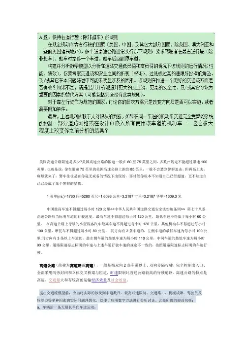
美国高速公路限速是多少?美国高速公路的限速一般在60至75英里之间,多数州规定不能超过限速100英里。
也就是说,你在限速75英里的美国高速公路上跑到85英里,一般不会遭到警察追击。
但再高上去,麻烦就来了,警车往往是在你毫无戒备的情况下出现的,那时候你根本不知道自己已经超速,更不知道自己已经成了某个警察的猎物。
1英里(mi.)=1760码=5280英尺=1.6093公里=3.2187市里=3.2187华里=1609.3米中国最高车速不得超过每小时120公里<<中华人民共和国道路交通安全法实施条例>> 第七十八条高速公路应当标明车道的行驶速度,最高车速不得超过每小时120公里,最低车速不得低于每小时60公里。
在高速公路上行驶的小型载客汽车最高车速不得超过每小时120公里,其他机动车不得超过每小时100公里,摩托车不得超过每小时80公里。
同方向有2条车道的,左侧车道的最低车速为每小时100公里;同方向有3条以上车道的,最左侧车道的最低车速为每小时110公里,中间车道的最低车速为每小时90公里。
道路限速标志标明的车速与上述车道行驶车速的规定不一致的,按照道路限速标志标明的车速行驶。
提出交通流模型前,应当将实际的涉及到车道数目、最高时速限制、交通路口、机械故障、驾驶员反应能力等多种因素的实际问题理想化,以便于应用数学方法进行分析讨论。
此处所做的假设包括:a.车辆沿一条无限长单向车道运动;b.车辆在单向车道内只能朝一个方向运动;c.单向车道是全封闭的,即没有供车辆驶入或者驶出的岔路口;d.车辆相对于此序列中的其他车辆位置不发生改变,即没有抛锚或超车的情况。
基于上述的假设,对作匀速运动的恒定密度车流而言,交通流变量的函数关系为:q=P0 0 (4)式中,P。
为车辆运动时的恒定密度;。
为车辆做匀速运动的速度。
实际的非恒定密度和非匀速运动的交通流仍然满足上述关系,其函数表达式为:g( ,t)=P( ,£)口( ,£车辆守恒方程由基本的交通流变量中所做的假设可知车辆的总体数目不会因观测点、观测时间的变化而变化。
PROBLEM A: The Keep-Right-Except-To-Pass RuleIn countries where driving automobiles on the right is the rule (that is, USA, China and most other countries except for Great Britain, Australia, and some former British colonies), multi-lane freeways often employ a rule that requires drivers to drive in the right-most lane unless they are passing another vehicle, in which case they move one lane to the left, pass, and return to their former travel lane.Build and analyze a mathematical model to analyze the performance of this rule in light and heavy traffic. You may wish to examine tradeoffs between traffic flow and safety, the role of under- or over-posted speed limits (that is, speed limits that are too low or too high), and/or other factors that may not be explicitly called out in this problem statement. Is this rule effective in promoting better traffic flow? If not, suggest and analyze alternatives (to include possibly no rule of this kind at all) that might promote greater traffic flow, safety, and/or other factors that you deem important.In countries where driving automobiles on the left is the norm, argue whether or not your solution can be carried over with a simple change of orientation, or would additional requirements be needed.Lastly, the rule as stated above relies upon human judgment for compliance. If vehicle transportation on the same roadway was fully under the control of an intelligent system – either part of the road network or imbedded in the design of all vehicles using the roadway – to what extent would this change the results of your earlier analysis?问题A 除超车保持右行规则在有些国家,驾驶机动车在右车道行驶(如美国,中国和除了英国,澳大利亚以及前英国殖民地国家的其它大多数国家),多车道的高速公路所使用的规则要求驾驶人员右车道行驶,除非他们要超车行驶,在此情况下他们先开到左侧车道,超车,然后在回到之前的行驶车道。
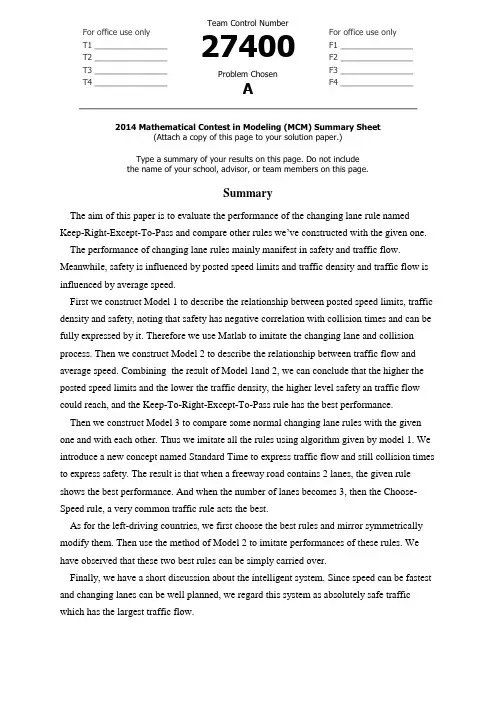
For office use onlyT1________________ T2________________ T3________________ T4________________Team Control Number27400Problem ChosenAFor office use onlyF1________________F2________________F3________________F4________________2014 Mathematical Contest in Modeling (MCM) Summary Sheet(Attach a copy of this page to your solution paper.)Type a summary of your results on this page. Do not includethe name of your school, advisor, or team members on this page.SummaryThe aim of this paper is to evaluate the performance of the changing lane rule named Keep-Right-Except-To-Pass and compare other rules we’ve constructed with the given one. The performance of changing lane rules mainly manifest in safety and traffic flow. Meanwhile, safety is influenced by posted speed limits and traffic density and traffic flow is influenced by average speed.First we construct Model 1 to describe the relationship between posted speed limits, traffic density and safety, noting that safety has negative correlation with collision times and can be fully expressed by it. Therefore we use Matlab to imitate the changing lane and collision process. Then we construct Model 2 to describe the relationship between traffic flow and average speed. Combining the result of Model 1and 2, we can conclude that the higher the posted speed limits and the lower the traffic density, the higher level safety an traffic flow could reach, and the Keep-To-Right-Except-To-Pass rule has the best performance.Then we construct Model 3 to compare some normal changing lane rules with the given one and with each other. Thus we imitate all the rules using algorithm given by model 1. We introduce a new concept named Standard Time to express traffic flow and still collision times to express safety. The result is that when a freeway road contains 2 lanes, the given rule shows the best performance. And when the number of lanes becomes 3, then the Choose-Speed rule, a very common traffic rule acts the best.As for the left-driving countries, we first choose the best rules and mirror symmetrically modify them. Then use the method of Model 2 to imitate performances of these rules. We have observed that these two best rules can be simply carried over.Finally, we have a short discussion about the intelligent system. Since speed can be fastest and changing lanes can be well planned, we regard this system as absolutely safe traffic which has the largest traffic flow.Team #27400 Page 1 of 161.Introduction1.1 Analysis to the problemThis problem can be divided into 4 requirements that we must meet, listed as follows:(1)Build a mathematical model to demonstrate the essence of Keep-Right-Except-To-Pass rule in light and heavy traffic;(2)Show the effects of other reasonable changing-lane rules or conditions by using themodified model built in the former requirement;(3)Determine whether the left-side-driving countries can use the same rule(s) withsimple mirror symmetric modification, or must add some requirements to guaranteethe safety or traffic flow;(4)Construct an intelligent traffic system which does not depend on humans’ compliance,and then compare the effects with earlier analysis.Therefore, this problem requires us to evaluate the performances of several changing-lane rules, especially the Keep-Right-Except-To-Pass rule while performances mainly manifest in traffic flow and safety. It is obvious that speed limit and the number of cars influent cars’ speed and then the performances of those rules.To solve requirement (2), we will use the same method as above. But all rules weconstructed should be discussed, imitated and compare with each other.To discuss the left-driving countries, we will conclude the best rules from requirement2 and apply to those countries. Then compare results with that of right-driving countries.If the results are totally the same, then those rules can be simply carried over with simple change. If not, additional requirement are needed.As for the intelligent system, we assume no collision will happen. So a simplediscussion is feasible.1.2 Crucial method for the problemTo imitate the process of changing lanes and collision, we will construct an algorithm named Changing-line and Collision. This will show the state of a number of car on the same stretch of freeway road, including going straight, changing lane to pass and traffic collision. The imitation process will be delivered on Matlab;2.Symbols and definitionSymbol Definition UnitσStandard Deviation of Speed miles/hmiles/hV85% Percentile of Normal85Distributionmiles/hV70% Percentile of Normal70DistributionDENS Traffic Density (Note: expressed by thenumber of cars) ST Standard Time \FLO Traffic Flow \CT Collision Times \3.General hypotheses for all models(1) All freeway roads contain either two or three lanes.(2) Overtaking Principle: the latter car must change lane and overtake the car right in front it if its speed is faster.(3) No violation of the rules.(4) The intelligent traffic system has no collision.(5) Road indicates one direction of the road.(6) Each cars remains constant speed no matter it goes straight or change lane.(7) Changing lane doesn’t cost time.(8) Given a traffic density, the average speed of cars is constant.(9) All discussions are confined to one stretch of road that is long enough to allow a series of cars to go across.4.Model establishment4.1 PreparationFirst, we must discuss what “changing-lane” is. For a two-lane road, if one car is going to change its lane to the left, then the right side lane “loses” one car and the left side lane “acquires” one, and vice versa. If the road contains three lanes, we can regard it as two “two-lane road”. This property also holds for an n-lane (n>2) road, which means we could regard it as (n-1) two-lane road. Therefore, changing-lane is the relation between two lanes. We just need to analyze a two-lane road to uncover the principle of changing lane and collision.Second, influence relationship figures are given below. In these figures, factors at lower level influence those at upper level. Safety will be expressed by collision times( ).Figure 1. General influence relationshipThird, we have constructed three additional changing-lane rules and shall describe these five rules in mathematical language. The original Keep-Right-Except-To-Pass rule is denoted Rule 1.Rule 1: Keep-Right-Except-To-Pass. If A B v v >, then car A goes left, overtakes car B and then gets back to the right lane.Figure 2. Rule one: Keep-Right-Except-To-PassRule 2: Free-Overtaking. If A B v v > and A C v v >, then car A changes lane to the left, passing B, and then to the right, passing C. And if there still exists a car D in front of A and A D v v >, car A will change to the left lane, pass D and then go straight. The following figure shows the case when the number of lanes is two, and it is identical for the case of 3 lanes.Figure 3. Rule 2: Free-OvertakingRule 3: Pass-Left. For a three-lane freeway road, if B A C v v v >>, then car A changes to the middle lane, and car B to the left lane, and finally they should get back to their original lane.Figure 4. Rule 3: Pass-LeftRule 4: Choose-Speed. Each lane of the road has a posted speed limit interval. We denote the left lane fast lane, right one slow lane and the middle one mid-lane. Drivers should choose lane according to their cars ’ speed.4.2 Model 1: Changing Lane and Collision Algorithm 4.2.1 Flow Diagram*To check Matlab code, please refer to Appendix 1. Note: we only use collision times to express safety.Figure 5. Flow Diagram of the Changing Lane and Collision Algorithm Comments:(1) The 1000*2 matrix stands for a stretch freeway road that contains two lanes;(2) Speed of cars is a series of random numbers which stands for the units they are to go forward each time;(3) Cars enter the road from the right lane.(4) If two cars collide, their speed will become zero but will not affect other cars. Accordingly, the position of collision will be valuated zero.To show how this algorithm works, we now give an example of a road, length 7 and five carswith different speed:Figure 6. An Example of the Algorithm4.2.2 Relationship between Average Speed, Standard Deviation of Speed and Posted Speed LimitsWe have mentioned in the last section that the speed of cars obeys normal distribution [3]. Now we deduce the relationship between ,μσ and PSL .Figure 7. Speed of cars obey normal distributionWe know from reference [4](page 15) that:857.6570.98V PSL =+⋅①The above foemula can be applied to all types of roads. Equation ② from reference [5](page 53):70-6.541+2.4V σ=⋅②Referring to the table of standard normal distribution, we have70V μσ-=0.52③ 85V μσ-=1.04④Considering formula ②③, we have=1.88-6.541μσ⑤Considering formula ①④, we have7.657+0.98=1.04PSL μσ-⑥Considering formula ⑤⑥, we have14.198+0.98=2.92PSLσ⑦0.98*=13.6012PSL μ-⑧Formula ⑦⑧ explains that the higher the posted speed limits, the greater the variance of speed and same to the average speed.0.9813.6012MU PSL =-⑨4.2.3 Process of ImitationWe now use control-variable method to describe the impact of traffic density and posted speed limits on safety. Therefore, we consider:(1) Traffic density being constant, the impact of variation of posted speed limits on safety; (2) Posted speed limits being constant, the impact of variation of traffic density on safety.When traffic density is constant:Table 1.Variation of Posted Speed LimitsPSL 50 60 70 80 90 100 μ 34.1481 40.4577 46.7673 53.0769 59.3865 65.6961 σ21.6432 24.9993 28.3555 31.7116 35.0678 38.424Figure 8. Variation of μ and σ along with Variation of PSLNote: SIGMA=σ, MU=μWhen posted speed limits is constant:Table 2.Variation of the number of carsThe number of cars 5 10 20 30 40 50Therefore we will acquire 6*6 groups of data when PSL is constant and 6*6 groups of data when traffic density is constant.4.3 Model 2: Relationship between Traffic Flow and Average SpeedIt is obvious that traffic flow is the function of average.We denote:=⋅+>FLO k MU c k(0)4.4 Model 3: Rules and Performances4.4.1 AnalysisIn section 4.1 we have listed four changing lane rules. Now we need to compare their effect and evaluate which rule has the best performance.According to the establishment of model 1, performances are fully expressed by safety and traffic flow, and safety has negative correlation with collision times. We can acquire the related data by imitation like model 1. However, since rules have changed, average speed of the road under different rules is different and is merely decided by PSL.Thus we introduce a new concept, namely, Standard Time(ST). Definition: time cost by each move of cars is called standard time. With this concept, we don’t need to calculate the real time cost by cars when going across a stretch of road, but count how many moves cars should make. Standard time has positive correlation with traffic flow, and we can denote:ST k FLO k=⋅>(0)4.4.2 Imitation ProcessConstruct a matrix. If the road contains two lanes, then the matrix size is 150*2; if it contains three lanes, then the size is 150*3. Arrange 40 random positions for each column vectors, and the numbers, as described before, obey normal distribution. Let other variables be constant, we discuss the impact of different rules on safety and traffic flow.Operations are as follows:(1) Distribute a series positions(40 for each column vector as described) for the matrix.(2) Valuate each position a number that obey normal distribution.(3) Apply one of the rules to the matrix. Those numbers will either “collide ” or “keep moving ” until all the position are valuated zero. (4) Record collision times and the spent standard time.(5) Apply another rule to the matrix, repeat steps (1) through (4).Statistically analyzing the data acquired and comparing the performances of different rules, we can decide advantages and disadvantages of each rule.4.4.3 Use the Method of 4.4.2 to Estimate Left-driving CountriesWe will conclude the best two rules and then apply the methods in section 4.4.2 to the left-driving country and estimate the performance of the two rules. Operation steps:(1) Mirror symmetrically modify the chosen rules; (2) Refer to the steps in section 4.4.2; (3) Compare with the results in 4.4.2.5. Model solution5.1 Model 1During the imitation process, we do the experiment for times for each case and then analyze all the results. We will show part of our statistical data. To view full data, please refer to Appendix 2.(1) Given DENS=30, the result is as follows:Table 3.Relationship between Changing Lane Times, Collision Times and PSL when DENS=30PSL Changing-lane times Average Collision TimesAverag-Line chart:Figure 9. Variation of Changing Lane Times and Collision Times along with Variation ofPSL(2) Given PSL=70, the result is as follows:Table 4.Relationship between Changing Lane Times, Collision Times and Number of Times whenPSL=70NumberChanging Lane Times Average Collision Time Average Line chart:Figure 10. Variation of Changing Lane Times and Collision Times along with Variation ofnumber of cars5.2 Model 2We know from formula ⑨, section 4.2.2 that0.9813.6012MU PSL =-Considering formula ⑨ and formula in 4.3, we have:0.9813.6012FLO k PSL k c =⋅-+5.3 Model 3The result of section 4.4.2 is given below:Table 5.Collision Times and Standard Time of each ruleRule →Rule 1 Rule 2(2Rule 3 Rule 2(3 Rule 4Extract the row of Average ST and Average CTTable 6.Average Collision Times and Average Standard Time of each rule The result of 4.4.3 is given below:Table 7.Collision Times and Standard Time of Rule 1 and Rule 4 Applied to Left-driving Countries6.Conclusion6.1 Conclusion of model 1 and 2We can conclude from model 1 that safety will decrease along with the growth oftraffic density. Safety will also decrease while the posted speed limits(PSL) is raised.However, comparing to PSL, traffic density has greater impact on safety while PSL can hardly influence safety.From model 2, we can conclude that traffic flow has liner growth along with the raise of PSL.The following table has summed up model 1 and 2.Table . 8Evaluation of Rule Performances in Different Road conditions6.2 Conclusion of model 3We can know from table 6 that when the number of lanes is 2, rule 1 is not very different from rule 2 in terms of traffic flow but is much safer than rule 2. When the number of lanes is 3, rule 3 is safest rule, but rule 4 will become both safe and efficient. Meanwhile, Free-Overtaking rule, actually meaning no rule, is most dangerous. Therefore, we have chosen rule 1 and rule 4 as the best rules.Result of section 4.4.3 is showed below. Note that original rules are listed on the left and modified on the right.Table .9Comparison between the Modified Rules and the OriginalFrom the table above, we can conclude that no difference between left-driving and right-driving countries. Therefore, those rules can be simply carried over with simple mirror symmetric modification.6.2 Conclusion of intelligent systemSince all the cars are controlled by a high-tech computer, we assume this system will never have an accident until the computer crashes. So every car reach their fastest speed, the order of overtaking can be calculated to avoid collision. Therefore, safety and traffic flow reach the highest level.7. References[1] Mark M. Meerschaert. Mathematical Modelling (Third Edition). Beijing: China Machine Press, 2008.12[2] Solomon. Accidents on Main Rural Highways Re la ted to Speed, Driver, and Vehicle[R]. Washing ton D. C: Federal Highway Administration, 1964[3] Lu Jian, Sun Xinglong, Daiyue. Regression analysis on speed distribution characteristics of ordinary road. Nanjing: Journal of Southeast University(Natural Science Edition), 2012.2 (in Chinese).[4] Wang Lijin. Research on Speed Limits and Operating Speed for Freeway. Beijing: Beijing University of Technology, 2011.5 (in Chinese).8. AppendixAppendix 1. Matlab Codeclear;clc;highway=zeros(1000,2);%define road%crash_times = 0;%define collition times%change_lane_times=0;%define change lane times%num_of_car=5; %definedefine number of car%MU=84.3898;SIGMA=20.4406;randspe=[];j=1;while j<=num_of_carx=round(normrnd(MU,SIGMA,1,1));if x>0randspe(j,1)=x; %define speed and gualentee %j=j+1;endx=0;endrandpla=[];for i=1:num_of_carx=ceil(rand(1)*1000);if find(randpla==x)x=ceil(rand(1)*1000); %define location and guarantee the car located in different place%endrandpla(i,1)=x;endfor i=1:num_of_carhighway(randpla(i,1),2)=randspe(i,1); %insert every car in different speed at diferent place %speed(i,1)=0;pla(i,1)=0;endinitialr_highway=highway; %record intialr-highway statement%disp(initialr_highway)disp('Aboveis the stateof initialr highway')while sum(sum(highway))~=0i=1;speed(1)=0; pla(1)=0;for j=1:length(highway) %Store the location and speed of each carif highway(j,2)~=0 ....to pla_matrix and speed_matrix separately%speed(i)=highway(j,2);pla(i)=j;i=i+1;endendcount=length(pla);while count>1 %When the differerce of two adjacent car's speed is greater than their distance,thenif speed(count)-speed(count-1)>=abs(pla(count)-pla(count-1)) ... the later car must change lane to the left% highway(pla(count),1)=highway(pla(count),2);highway(pla(count),2)=0;change_lane_times=change_lane_times+1;endcount=count-1;endlane_changed= highway; %record lane_changed highway statement%disp(lane_changed)disp('Aboveis the state of after-changed lane highway ')k=1;pas_spe(1)=0;pas_pla(1)=0;for j=1:length(highway)if highway(j,1)~=0pas_spe(k)=highway(j,1);pas_pla(k)=j;k=k+1;endendcount=length(pas_pla); %delete crashed car%while count>1if pas_spe(count)-pas_spe(count-1)>=abs(pas_pla(count)-pas_pla(count-1))highway(pas_pla(count),1)=0;highway(pas_pla(count-1),1)=0;crash_times=crash_times+1;endcount=count-1;endaft_adjust = highway;disp(aft_adjust)disp('Above is after adjusted highway')for i=1:length(highway)for j=1:2if i-highway(i,j)>0highway(i-highway(i,j),j)=highway(i,j);%move forward%endhighway(i,j)=0;endendfor i=1:length(highway)if highway(i,1)~=0&&highway(i,2)==0%back to right%highway(i,2)=highway(i,1);highway(i,1)=0;endendback_to_right = highway; %record lane_changed highway statement%disp(back_to_right);disp('Aboveis the state of back_to_right lane highway.');pla=0;speed=0;pas_pla=0;pas_spe=0;endfprintf('change_lane_time ','\n');disp(change_lane_times)fprintf('crash_time ','\n');disp(crash_times)Appendix 2. Data of ImitationPSL Change lane times Mean Crash times MeanNumberof cars=5 50 2 2 2 2.0 0 0 0 0.0 60 3 2 3 2.7 0 0 0 0.0 70 1 0 1 0.7 0 0 0 0.0 80 2 0 1 1.0 0 0 0 0.0 90 0 0 3 1.0 0 0 0 0.0 100 1 3 2 2.0 0 0 0 0.0Numberof 50 7 5 11 7.7 0 0 0 0.0 60 8 11 8 9.0 0 1 0 0.3cars=10 70 10 6 7 7.7 1 0 1 0.780 6 7 10 7.7 0 1 1 0.790 4 7 4 5.0 1 2 0 1.0100 6 3 3 4.0 1 1 1 1.0Numberof cars=20 50 47 29 38 38.0 1 2 2 1.7 60 30 34 20 28.0 2 0 1 1.0 70 15 17 22 18.0 0 2 3 1.7 80 18 22 16 18.7 0 2 1 1.0 90 20 10 22 17.3 1 1 2 1.3 100 21 15 13 16.3 2 2 1 1.7Numberof cars=30 50 61 60 48 56.3 5 4 2 3.7 60 46 42 45 44.3 4 1 2 2.3 70 42 38 48 42.7 4 5 3 4.0 80 43 32 47 40.7 2 5 5 4.0 90 32 41 33 35.3 3 4 5 4.0 100 26 27 24 25.7 2 2 4 2.7Numberof cars=40 50 65 100 74 79.7 8 4 8 6.7 60 56 77 75 69.3 5 8 3 5.3 70 53 64 62 59.7 4 5 5 4.7 80 52 60 60 57.3 3 7 3 4.3 90 44 53 48 48.3 5 4 4 4.3 100 43 50 38 43.7 1 7 0 2.7Numberof cars=50 50 82 86 106 91.3 12 12 10 11.3 60 80 68 72 73.3 10 9 13 10.7 70 82 75 81 79.3 8 7 10 8.3 80 61 72 58 63.7 9 7 11 9.0 90 57 54 54 55.0 6 7 11 8.0 100 64 50 51 55.0 7 9 8 8.0PSL=705 1 0 1 0.7 0 0 0 0.0 10 1067 7.7 1 0 1 0.7 20 15 17 22 18.0 0 2 3 1.7 30 42 38 48 42.7 4 5 3 4.0 40 53 64 62 59.7 4 5 5 4.7 50 82 75 81 79.3 8 7 10 8.3PSL Change lanetimescollisiontimesDensityChange lanetimescollisiontimes50 56.33333333 3.666666667 5.0 0.666666667 060 44.33333333 2.333333333 10.0 7.666666667 0.666666667 70 42.66666667 4 20.0 18 1.666666667 80 40.66666667 4 30.0 42.66666667 490 35.33333333 4 40.0 59.66666667 4.666666667 100 25.66666667 2.666666667 50.0 79.33333333 8.333333333。
2010 MCM ProblemsPROBLEM A: The Sweet SpotExplain the “sweet spot” on a baseball bat.Every hitter knows that there is a spot on the fat part of a baseball bat where maximum power is transferred to the ball when hit. Why isn’t this spot at the end of the bat? A simple explanation based on torque might seem to identify the end of the bat as the sweet spot, but this is known to be empirically incorrect. Develop a model that helps explain this empirical finding.Some players believe that “corking” a bat (hollowing out a cylinder in the head of the bat and filling it with cork or rubber, then replacing a wood cap) enhances the “sweet spot” effect. Augment your model to confirm or deny this effect. Does this explain why Major League Baseball prohibits “corking”?Does the material out of which the bat is constructed matter? That is, does this model predict different behavior for wood (usually ash) or metal (usually aluminum) bats? Is this why Major League Baseball prohibits metal bats?MCM 2010 A题:解释棒球棒上的“最佳击球点”每一个棒球手都知道在棒球棒比较粗的部分有一个击球点,这里可以把打击球的力量最大程度地转移到球上。
clfclear all%build the GUI%define the plot buttonplotbutton=uicontrol('style','pushbutton',...'string','Run', ...'fontsize',12, ...'position',[100,400,50,20], ...'callback', 'run=1;');%define the stop buttonerasebutton=uicontrol('style','pushbutton',...'string','Stop', ...'fontsize',12, ...'position',[200,400,50,20], ...'callback','freeze=1;');%define the Quit buttonquitbutton=uicontrol('style','pushbutton',...'string','Quit', ...'fontsize',12, ...'position',[300,400,50,20], ...'callback','stop=1;close;');number = uicontrol('style','text', ...'string','1', ...'fontsize',12, ...'position',[20,400,50,20]);%CA setupn=100;%数据初始化z=zeros(1,n);%元胞个数z=roadstart(z,5);%道路状态初始化,路段上随机分布5辆cells=z;vmax=3;%最大速度v=speedstart(cells,vmax);%速度初始化x=1;%记录速度和车辆位置memor_cells=zeros(3600,n);memor_v=zeros(3600,n);imh=imshow(cells);%初始化图像白色有车,黑色空元胞set(imh, 'erasemode', 'none')axis equalaxis tightstop=0; %wait for a quit button pushrun=0; %wait for a drawfreeze=0; %wait for a freeze(冻结)while (stop==0)if(run==1)%边界条件处理,搜素首末车,控制进出,使用开口条件a=searchleadcar(cells);b=searchlastcar(cells);[cells,v]=border_control(cells,a,b,v,vmax); i=searchleadcar(cells);%搜索首车位置for j=1:iif i-j+1==n[z,v]=leadcarupdate(z,v);continue;else%======================================加速、减速、随机慢化 if cells(i-j+1)==0;%判断当前位置是否非空continue;else v(i-j+1)=min(v(i-j+1)+1,vmax);%加速%=================================减速k=searchfrontcar((i-j+1),cells);%搜素前方首个非空元胞位置if k==0;%确定于前车之间的元胞数d=n-(i-j+1);else d=k-(i-j+1)-1;endv(i-j+1)=min(v(i-j+1),d);%==============================%减速%随机慢化v(i-j+1)=randslow(v(i-j+1));new_v=v(i-j+1);%======================================加速、减速、随机慢化%更新车辆位置z(i-j+1)=0;z(i-j+1+new_v)=1;%更新速度v(i-j+1)=0;v(i-j+1+new_v)=new_v;endendendcells=z;memor_cells(x,:)=cells;%记录速度和车辆位置memor_v(x,:)=v;x=x+1;set(imh,'cdata',cells)%更新图像%update the step number diaplaypause(0.2);stepnumber = 1 + str2num(get(number,'string'));set(number,'string',num2str(stepnumber))endif (freeze==1)run = 0;freeze = 0;enddrawnowend///////////////////////////////////////////////////////////////////////Function[new_matrix_cells,new_v]=border_control(matrix_cells,a,b,v,vmax) %边界条件,开口边界,控制车辆出入%出口边界,若头车在道路边界,则以一定该路0.9离去n=length(matrix_cells);if a==nrand('state',sum(100*clock)*rand(1));%¶¨ÒåËæ»úÖÖ×Óp_1=rand(1);%产生随机概率if p_1<=1 %如果随机概率小于0.9,则车辆离开路段,否则不离口matrix_cells(n)=0;v(n)=0;endend%入口边界,泊松分布到达,1s内平均到达车辆数为q,t为1sif b>vmaxt=1;q=0.25;x=1;p=(q*t)^x*exp(-q*t)/prod(x);%1s内有1辆车到达的概率rand('state',sum(100*clock)*rand(1));p_2=rand(1);if p_2<=pm=min(b-vmax,vmax);matrix_cells(m)=1;v(m)=m;endendnew_matrix_cells=matrix_cells;new_v=v;///////////////////////////////////////////////////////////////////////function [new_matrix_cells,new_v]=leadcarupdate(matrix_cells,v)%第一辆车更新规则n=length(matrix_cells);if v(n)~=0matrix_cells(n)=0;v(n)=0;endnew_matrix_cells=matrix_cells;new_v=v;///////////////////////////////////////////////////////////////////////function [new_v]=randslow(v)p=0.3;%慢化概率rand('state',sum(100*clock)*rand(1));%¶¨ÒåËæ»úÖÖ×Óp_rand=rand;%产生随机概率if p_rand<=pv=max(v-1,0);endnew_v=v;///////////////////////////////////////////////////////////////////////function [matrix_cells_start]=roadstart(matrix_cells,n)%道路上的车辆初始化状态,元胞矩阵随机为0或1,matrix_cells初始矩阵,n初始车辆数k=length(matrix_cells);z=round(k*rand(1,n));for i=1:nj=z(i);if j==0matrix_cells(j)=0;elsematrix_cells(j)=1;endendmatrix_cells_start=matrix_cells;///////////////////////////////////////////////////////////////////////function[location_frontcar]=searchfrontcar(current_location,matrix_cells)i=length(matrix_cells);if current_location==ilocation_frontcar=0;elsefor j=current_location+1:iif matrix_cells(j)~=0location_frontcar=j;break;elselocation_frontcar=0;endendend///////////////////////////////////////////////////////////////////////function [location_lastcar]=searchlastcar(matrix_cells)%搜索尾车位置for i=1:length(matrix_cells)if matrix_cells(i)~=0location_lastcar=i;break;else %如果路上无车,则空元胞数设定为道路长度location_lastcar=length(matrix_cells);endend///////////////////////////////////////////////////////////////////////function [location_leadcar]=searchleadcar(matrix_cells)i=length(matrix_cells);for j=1:iif matrix_cells(i-j+1)~=0location_leadcar=i-j+1;break;elselocation_leadcar=0;endend///////////////////////////////////////////////////////////////////////function [v_matixcells]=speedstart(matrix_cells,vmax)%道路初始状态车辆速度初始化v_matixcells=zeros(1,length(matrix_cells));for i=1:length(matrix_cells)if matrix_cells(i)~=0v_matixcells(i)=round(vmax*rand(1));endend。
2014 ICM Problem使用网络来测量的影响和冲击Using Networks to Measure Influence and Impact确定学术研究的影响力的一种方法是构建和测量引文或合著者网络的属性.共同创作的文章通常意味着研究者之间的影响力有了重要的连接。
其中最有名的学术合著者是20世纪的数学家保罗·埃尔德什(Paul Erdös)他拥有超过500共同作者,并发表了超过1400的技术研究论文。
说埃尔德什(Erdös)是具有学科交叉特点的网络科学(science of networks)这一新兴研究的奠基人之一或许具有讽刺意味,或者也不。
特别是1959年,他和阿尔弗雷德的共同撰写的论文“关于随机图”(“On Random Graphs”)的发表,使得埃尔德什的作为合作者的角色在数学领域变得十分重要以至于数学家们经常会通过分析埃尔德什数量惊人的合作者来衡量自己与埃尔德什联系的紧密程度(their closeness to Erdös)。
(see the website http://www.oakla /enp/ )保罗.埃尔德什作为一个天才的数学家,天才的问题解决者,和著名合作者的不寻常和令人着迷的故事公布也在了许多书籍和在线网站上。
(例如,/Biographies/Erdos.html ).也许,他的生活方式就是经常和他的合作者待在一起或者住在一起。
或者把钱给他的学生作为解决问题的奖励,从而使他的合作蓬勃发展,并帮助他在数学的几个领域里建立了具有惊人影响力的网络。
为了衡量诸如埃尔德什等人产生的影响力,已经有了一些基于网络评价的工具(network-based evaluation tools)。
即是利用共同作者和引文数据来确定学者,出版物和学术期刊的影响因子,比如:科学文献索引(Science Citation Index,SCI的),H- factor(一种评价学术成就的新方法)Impact factor (期刊影响因子,SCI),Eigenfactor等等。
2014National English Competitionfor College Students(Level A-Preliminary)参考答案及作文评分标准Part I Listening Comprehension(30marks)Section A(5marks)1—5BACCASection B(10marks)6—8CCD9—10CB11—15ADBCASection C(5marks)16—20BDCDASection D(10marks)munication22.surrounding a message23.directly24.implied25.very different meanings26.Low27.message itself28.explicit29.External factors30.the same wayPart II Vocabulary,Grammar&Cultures(15marks)Section A(10marks)31—35ABCCB36—40CCDACSection B(5marks)41—45CAABBPart III Cloze(10marks)46.for47.hono(u)r48.which49.feasibility50.replacement51.original52.auditorium53.theatrical54.also55.formerlyPart IV Reading Comprehension(35marks)Section A(5marks)56—60TTFTTSection B(10marks)61—65EDAFBSection C(10marks)66.They are used to buy things with“loyalty points”people haven’t earned yet,but which then have to be repaid with increased customer loyalty.67.To achieve different aspects of local sustainability.68.People in the community are willing to help others and they get paid with Time dollars in turn.69.New ways to pay and how they change people’s life.70.Money issued by supermarkets and airlines,like frequent-flier miles and incentive cards;LETS money; local currencies,like Time dollars and Hours.Section D(10marks)71.media cultural exports73.flow of information74.promote multiculturalism75.difficult to resistPart V Translation(15marks)Section A(5marks)76.海洋覆盖地球表面的四分之三,地球上维持生命的氧气,90%来自海洋,整个天气系统变化的动力也是海洋。
Acta Mech.Sin.(2011)27(2):228–236DOI10.1007/s10409-011-0419-yRESEARCH PAPERA continuum trafficflow model with the considerationof coupling effect for two-lane freewaysDi-Hua Sun·Guang-Han Peng·Li-Ping Fu·Heng-Pan HeReceived:5December2008/Revised:22April2010/Accepted:6May2010©The Chinese Society of Theoretical and Applied Mechanics and Springer-Verlag Berlin Heidelberg2011Abstract A new higher-order continuum model is proposed by considering the coupling and lane changing effects of the vehicles on two adjacent lanes.A stability analysis of the proposed model provides the conditions that ensure its lin-ear stability.Issues related to lane changing,shock waves and rarefaction waves,local clustering and phase transition are also investigated with numerical experiments.The sim-ulation results show that the proposed model is capable of providing explanations to some particular traffic phenomena commonly observable in real trafficflows.Keywords Two-lane traffic·Two delay time scales model·Numerical simulation·Coupling effect·Phase transition The project was supported by the National High Technology Re-search and Development Program of China(863)(511-0910-1031) and the National“10th Five-Year”Science and Technique Impor-tant Program of China(2002BA404A07).D.-H.Sun·G.-H.Peng()College of Automation,Chongqing University,400030Chongqing,Chinae-mail:pengguanghan@L.-P.FuDepartment of Civil&Environmental Engineering,University of Waterloo,Waterloo,Ontario N2L3G1,CanadaH.-P.HeCollege of Automation,Chongqing University,400030Chongqing,China 1IntroductionLWR theory is the earliest and most fundamentalfirst-order continuum traffic model proposed by Lighthill and Whitham[1]and Richards[2]independently.According to this theory,trafficflows on a long homogeneous freeway are governed by the following conservation equation∂k∂t+∂q∂x=s(x,t),(1) where k is traffic density,q is trafficflow rate,x is space,t is time and s(x,t)isflow generation rate.When there is no on-offramp,s(x,t)=0;otherwise,s(x,t) 0.The equivalent flow-density relationship betweenflow rate q and density k isq=ku.(2) For the speed u,as in LWR,the existence of an equilib-rium speed-density relationship is assumedu=u e(k).(3) According to the above three equations,analytical so-lutions can be obtained.Some trafficflow problems,such as shock waves and traffic jams,can be addressed from these solutions.However,the LWR model cannot be used to describe correctly the trafficflows in nonequilibrium states since the equilibrium relationship between speed and density is a1ways assumed in the equilibrium speed–density equa-tion(3).Many scholars have proposed high-order continuum trafficflow models that incorporate a dynamics equation or momentum equation to represent general car-following be-havior[3–11].This momentum equation takes theacceler-A continuum trafficflow model with the consideration of coupling effect for two-lane freeways229 ation and inertia of driving into account.Hence,the high-order models make up for some deficiencies in the simplecontinuum models and improve their ability to reproducecomplex traffic behavior.However,the existing high-order models have a fun-damentalflaw that one of the characteristic speeds result-ing from the momentum and conservation equations is lagerthan the macroscopicflow speed.This implies that vehicleswould affect the vehicles in front of them[12].This evi-dently violates the anisotropy of trafficflow and does notaccord with the real traffic.On the basis of their full velocity difference(FVD)car-following model[13],Jiang et al.[12]proposed a new dy-namic equation in which the density gradient term is replacedby a speed gradient term.Recently,Jiang and Wu[14]fur-ther analyzed the structural properties of the solutions ofthe speed gradient trafficflow model.The solutions showedthat the model’s characteristic speeds are not lager than themacroscopicflow speed,hence vehicles respond only to theirfrontal stimulus.But the propagation speed of disturbancec0in this model is a constant,independent of the density.In fact,the propagation speed of disturbance in a Payne-Whitham-like model should depend on the density[15,16].Concerning the relationship between disturbance propaga-tion speed and density,with two delay time scales taken intoaccount,Xue and Dai[17]improved the model by treatingc0as a function of the density,with which the undesirable“wrong-way travel”phenomenon and gas-like behavior areeliminated and the formation and diffusion of traffic shockcan be better simulated.In the above models,the following car is not allowedto overtake the leading car.Hence,these models are appli-cable only to the trafficflow on freeways with single lane.Daganzo[18]developed a continuum theory of traffic dy-namics for freeways with two lanes allocated for two sortsof vehicles(lane1for faster vehicles and lane2for slowervehicles).The theory defines the conservation equation as∂P ∂t +∂Q∂x=S,(4)where P=(k1,k2)T,Q=[q1(k1,k2),q2(k1,k2)]T,(s21−s12,s12−s21)T,k m and q m represent the traffic density and the flow rate on lane m(m=1,2),respectively,s mn represents lane changing rate from lane m to lane n.Daganzofirst stud-ied the possible relationships between the velocities and the densities based on the density ratio of the two lanes,then for-mulated the trafficflow models for each of totally four k1−k2 regions.To carry out analyses graphically,Daganzo adopted simple continuum model only;hence his approach cannot be used to describe the non-equilibrium trafficflow dynamics. Wu[19]proposed a multi-lane traffic model,considering the specific traffic conditions in Chinese cities(e.g.,untidyflows and lower speeds on roads),but Wu’s model tends to equalize all lanes’densities through averaging them.This conflicts with the real traffic since the density on the lane allocated for faster vehicles is generally less than that on the lane al-located for slower vehicles.Tang and Huang[20,21]lately developed a continuum model for freeways with two lanes which integrates the momentum equation proposed by Jiang et al.[12]to the Daganzo’s modeling framework for multi-lane trafficflow[18].However,this model allows only the faster vehicles to change lanes.Recently,Huang and Tang et al.[22]further extended the work of Tang and Huang[20,21] by allowing that vehicles on both lanes to change their lanes according to the traffic condition on the spot and in real time, which contains the speed gradient-based momentum equa-tions derived from a car-following theory suited to two-lane trafficflow.Tang and Jiang et al.[23]also extended the speed gradient model to trafficflow on two-lane freeways. But the coupling effect of the interactions between vehicles on two lanes has not been taken into account in these models.In this paper,we extend the two delay time scales model proposed by Xue et al.[17]to describe asymmetric two-lane traffic with the consideration of coupling effect,allowing that vehicles on both lanes to change their lanes according to the traffic condition on the spot and in real time.We also in-vestigate lane changing rate resulting in the shock waves and rarefaction waves and the local cluster wave effect in two-lane freeways.The paper is organized as follows.In Sect.2,we es-tablish a continuum model with anisotropy by introducing the drivers’reaction time t r and the vehicle relaxation time T into the forward anticipation speed with the consideration of coupling effect on both lanes;thus the propagation speed of a small disturbance is related to the density.In Sect.3,we an-alyze the linear stability of the new model and give necessary and sufficient conditions for ensuring the stability.Numeri-cal results are presented in Sect.4to validate the theoretical analysis,and some nonequilibrium phenomena are investi-gated,such as small disturbance instability,shock waves and rarefaction waves,local cluster waves and phase transition. Section5concludes the paper with a summary of majorfind-ings and directions for future research.2Modeling and analysisThe two delay time scale model proposed by Xue is based on the assumption of forward anticipation[17],in which the stream speed u in the relaxation time T just reaches the an-ticipated value u e corresponding to the density in time t+t r at location x+ut r,where t r is driver reaction time.The speed-density relationship can be expressed as followsu(x+uT,t+T)=u e(k(x+ut r,t+t r)).(5) Using the Taylor series expansion of Eq.(5),applying Eq.(1) and referring to Ref.[17],we get∂u∂t+(u−c(k))∂u∂x=u e(k)−uT,c(k)=−kt rTd u ed k≥0,T=T0[1+E/(1+(k/k M)θ)],(6)230 D.-H.Sun,et al. where c(k)is the“sonic speed”in trafficflow,at which smalldisturbances propagate relative to a moving traffic stream.The relaxation time T is a nonlinear function of the densityk.And k M is the critical density,T0is the constant reactiontime,θis a parameter(θ>0),and E is a constant(E>0)thatdenotes the difference in reaction times between congestedand uncongested traffic situations.As k→0,T→(E+1)T0;when k>k M,T>T0.This means that at high density levelsthe relaxation time is smaller,and at low density levels therelaxation time is larger.On two-lane freeways,the lane changing behaviour willoccur.To model this effect,the interactions between vehicleson two lanes,i.e.the coupling effect between two lanes,mustbe taken into account to describe theflow rate changing fromthe other lane.So a coupling effect term is added to Eq.(5)to describe theflow rate changing to the other lane.u m(x+u m T m,t+T m)=u e m[k m(x+u m t r m,t+t r m),βnm k n],m,n=1,2,and m n.(7)Equation(7)means that the stream speed u m in the relaxationtime T m just reaches the anticipated value u e m(u e m is func-tions of k1and k2)corresponding to the density in time t+t r mat the location x+ut r m on lane m,where t r m is driver reactiontime on lane m.And hereβnm is coupling coefficient fromlane n to lane m.On the basis of principle of coupling inter-action,we considerβnm=βmn=β.Using the Taylor seriesexpansion of Eq.(7)and neglecting higher-order terms,wegetu m(x,T m)+∂u m∂t T m+u m T m∂u m∂x+O(T2m)=u e m(k m,βk n)+∂u e m∂k m×t r m∂k m∂t+u m t r m∂k m∂x+O(t2r m).(8)Equation(8)can be rearranged as∂u m ∂t +u m∂u m∂x=u e m(k m,βk n)−u mT m+t r mT m∂u e m∂k m×∂km∂t+u m∂k m∂x.(9)Applying Eq.(4),we have∂u m ∂t +(u m−c m0)∂u m∂x=u e m(k m,βk n)−u mT m+γm s nm−γm s mn,c m0=−k m t r mT m∂u e m(k m,βk n)∂k m≥0,γm=t r mT m ∂u e m(k m,βk n)∂k m.(10)The dynamics model for two-lane traffic consists of the fol-lowing equations∂k m ∂t +∂q m∂x=s nm(x,t)−s mn(x,t),(11)∂u m ∂t +(u m−c m0)∂u m∂x=u e m(k m,βk n)−u mT m+γm s nm−γm s mnm,n=1,2,and m n,(12)where c m0=−k m t r m Tm∂u e i(k m,βk n)∂k m≥0represents the propaga-tion speed of the disturbance on lane m.Note that the modelgiven by Eqs.(11)and(12)for a specific lane is formally thesame as the continuum model proposed by Xue[17](whenβ=0and S=0on a single lane).However,attention shouldbe paid to such a difference that all the velocities in Eqs.(11)and(12)are functions of k1and k2.According to Liu’sidea[24]and Tang’s method[23],we suppose the analogyterms of lane changing rate have the form as followss12=aQ e1k1(1−(k2/k2jam)σ),(13)s21=a(1+b(Q e1−Q e2))×Q e2k2(1−(k1/k1jam)φ),(14)where Q e i is the equilibriumflow(Q e i=ku e i(k))andσ,φarethe parameters that reflect the intensity of the lane-changeeffect from one lane to another,0≤σ,φ≤1,and depend onthe condition of road.The special case of Q e1=Q e2corre-sponds to symmetric lane changing rules,while Q e1 Q e2corresponds to asymmetric lane changing rules;a and b areconstant parameters,k i jam is the jam density of lane i.In real traffic,the lane changing rate,say from lane1to2,should be zero when either k2=k2jam(lane2is in com-plete jam)or k1=0(there is no vehicle on lane1).Further-more,it obviously depends on the equilibrium speed densityrelationship on the present lane and on the coupling densityof the other lane.These properties are fulfilled in Eqs.(13)and(14).We rewrite system(11)and(12)as follows∂V∂t+A∂V∂x=E,(15)whereV=⎧⎪⎪⎪⎪⎪⎪⎪⎪⎪⎨⎪⎪⎪⎪⎪⎪⎪⎪⎪⎩k1u1k2u2⎫⎪⎪⎪⎪⎪⎪⎪⎪⎪⎬⎪⎪⎪⎪⎪⎪⎪⎪⎪⎭,A=⎡⎢⎢⎢⎢⎢⎢⎢⎢⎢⎢⎢⎢⎢⎢⎢⎢⎢⎢⎢⎢⎣u1k1000u1−c100000u2k2000u2−c20⎤⎥⎥⎥⎥⎥⎥⎥⎥⎥⎥⎥⎥⎥⎥⎥⎥⎥⎥⎥⎥⎦,E=⎡⎢⎢⎢⎢⎢⎢⎢⎢⎢⎢⎢⎢⎢⎢⎢⎢⎢⎢⎢⎢⎣s21−s12(u e1−u1)/T1+γ1s21−γ1s12s12−s21(u e2−u2)/T2+γ2s12−γ2s21⎤⎥⎥⎥⎥⎥⎥⎥⎥⎥⎥⎥⎥⎥⎥⎥⎥⎥⎥⎥⎥⎦.(16)Comparing our new model with other continuum modelspresented by Daganzo[18],we can see that the new modelincludes two new motion equations,in which the speed gra-dient term replaces the density gradient term as theantici-A continuum tra ffic flow model with the consideration of coupling e ffect for two-lane freeways 231pation term with c i 0=c (k i ).This replacement in the new model solves the characteristic speed problem that exists in the previous high-order models and therefore enables the new model to satisfy the anisotropic property of tra ffic flows.Next we apply matrixes to analyze character speeds of the system (15).The eigenvalues,λ,of matrix A are found by setting det(A −λI )=0,(17)where I is identity matrix.From Eq.(17),we have λ11=u 1,λ12=u 1−c 10,λ21=u 2,λ22=u 2−c 20.From the above-mentioned,c i 0≥0(i =1,2),which means that the character speeds of each subsystem are not larger than their macroscopic flow speeds,which shows that on each lane the rear disturbances cannot propagate forward.However,it does not guarantee that in a system consisting of two lanes the rear disturbance will not a ffect the driving behavior of the leading vehicle because lane changing is al-lowed in these two-lane tra ffic system.3Linear stablity conditionAccording to the method introduced by Huang et al.[22]and Tang et al.[23],the steady state solutions of the ex-tended two delay time scales model can be obtained by set-ting the derivative terms in Eqs.(11)and (12)to zero.It means here s nm −s mn =0(m ,n =1,2).For lane m (=1,2),let k ∗m and u ∗m be the steady-state solutions of the model (11)–(12),k m =k ∗m +ξm and u m =u ∗m +εm be the perturbed solu-tions,where ξm =ξm (x ,t )and εm =εm (x ,t )represent smallsmooth perturbations to the steady-state solutions.Substitut-ing k m =k ∗m +ξm and u m =u ∗m +εm into Eqs.(11)and (12),taking the Taylor series expansions at the point (k ∗m ,u ∗m )andneglecting the higher order terms of ξm and εm ,we obtain the following equations∂ξm ∂t +u ∗m ∂ξm ∂x +k ∗m ∂εm ∂x=0,m =1,2,(18)∂ε1∂t + u ∗1−c 10 ∂ε1∂x =a ξ1+b ξ2−ε1T 1,(19)∂ε2∂t + u ∗2−c 20 ∂ε2∂x =c ξ1+d ξ2−ε2T 2,(20)where a =∂u e1(k ∗1,βk ∗2)/∂k 1,b =∂u e1(k ∗1,βk ∗2)/∂k 2,c =∂u 2e (βk ∗1,k ∗2)/∂k 1,d =∂u 2e (βk ∗1,k ∗2)/∂k 2.Eliminating ε1and ε2in Eqs.(18)–(20),we obtain(∂t +c 1∂x )ξ1=−T 1(∂t +c 11∂x )(∂t +c 12∂x ) ξ1,(21)(∂t +c 2∂x )ξ2=−T 2 (∂t +c 21∂x )(∂t +c 22∂x )ξ2,(22)where c 1=u ∗1+k ∗1(ad −bc )/d ,c 2=u ∗2+k ∗2(ad −bc )/a ,c 11=u ∗1−c 10,c 12=u ∗1,c 21=u ∗2−c 20,c 22=u ∗2.According to the traditional way of linear stability anal-ysis,and substituting ξi (x ,t )=ξi 0exp i (γx −wt ),i =1,2into Eqs.(21)and (22),we can show that(−iw +ic 1γ)ξ1=−T 1(−iw +c 11i γ)(−iw +c 12i γ) ξ1,(23)(−iw +ic 2γ)ξ2=−T 2(−iw +c 21i γ)(−iw +c 22i γ) ξ2.(24)Because ξi is non-trivial solution of Eqs.(23)and (24),we must have−T (w −c 11γ)(w −c 12γ)+i (w −c 1γ)=0,(25)−T (w −c 21γ)(w −c 22γ)+i (w −c 2γ)=0.(26)It is obvious that the solution is stable if and only if the imaginary part of both roots w of Eqs.(25)and (26)are non-positive.For such equations as Eqs.(25)and (26),Whitham [25]and Zhang [26]have already veri fied that the requirement for this is c 11≤c 1≤c 12,(27)c 21≤c 2≤c 22.(28)Inequalities (27)and (28)are the criteria of stability.Whenone of the conditions (27)and (28)is violated,tra ffic in-stability will occur.Also inequalities (27)and (28)shows that one lane’s stability is a ffected by its lateral lane’s traf-fic density.Equations (21)and (22)show that linear wave is second-order wave.The second-order wave propagation speed is very similar to the characteristic speed.But the steady-state solutions u ∗i replace flow u i for linear stability analysis.And first-order wave of both lanes propagates at the same wave speed c 1and c 2.However,higher-order wave propagates at di fferent speeds,which depends on character-istic speeds.Second-order wave speeds,c 11and c 12,c 21and c 22,determine the fastest and slowest propagation speed of perturbation information for second order equation of two lane system.However,the propagation speed of first-order wave c i is the propagation speed of main perturbation in-formation.Thus,when the inequality c 11≤c 1≤c 12and c 21≤c 2≤c 22,both are satis fied at the same time,the prop-agating perturbations do not con flict with each other,which assures the stability of the system.When c i ≥c i 2or c i ≤c i 1,the propagation speed of main perturbation information is greater than the highest speed of information propagation or less than the lowest speed of information propagation,and the propagating perturbations will con flict with each other,which results in inextricable competition between first-and second-order wave.Only the inextricable competition leads to instability of the system.4Numerical simulationIn this section,using the finite di fference method,we numer-ically solve the model to demonstrate the model’s ability of capturing complex tra ffic phenomena.Let index j represent the time interval and index i the road section,then thedif-232 D.-H.Sun,et al. ference equations corresponding to Eqs.(11)and(12)are asfollowsk(j+1) m(i)=k(j)m(i)+ΔtΔx k(j)m(i)u(j)m(i)−u(j)m(i+1)+ΔtΔx u(j)m(i)k(j)m(i−1)−k(j)m(i)+Δts(j)nm(i)−Δts(j)mn(i),m,n=1,2.(29)(1)When traffic is heavy,u(j)m(i)<c m0,u(j+1) m(i)=u(j)m(i)+ΔtΔxc m0−u(j)m(i)u(j)m(i+1)−u(j)m(i)+ΔtT1u e m−u(j)m(i)+γmΔts(j)nm(i)−γmΔts(j)mn(i),m,n=1,2(30)(2)When traffic is light,u(j)m(i)≥c m0,u(j+1) m(i)=u(j)m(i)+ΔtΔxc m0−u(j)m(i)u(j)m(i)−u(j)m(i−1)+ΔtT2u e m−u(j)m(i)+γmΔts(j)nm(i)−γmΔts(j)mn(i),m,n=1,2(31)4.1Shock waves and rarefaction wavesIn order to investigate congestion and dissipation of the traf-ficflow,we use two Riemann initial conditions[17,21].(1)⎧⎪⎪⎨⎪⎪⎩k11u=0.03,k12u=0.04,⎧⎪⎪⎨⎪⎪⎩k11d=0.12,k12d=0.18,(32a)(2)⎧⎪⎪⎨⎪⎪⎩k21u=0.12,k22u=0.18,⎧⎪⎪⎨⎪⎪⎩k21d=0.03,k22d=0.04,(32b)where k11u ,k12u,k11d,k12dand k21u,k22u,k21d,k22dare,the up-stream and downstream densities of two lanes,respectively. Equation(32a)corresponds to the appearance of shock waves when free-flow traffic meets stopped vehicles,while Eq.(32b)corresponds to the rarefaction wave as a queue dis-solves.Two initial conditions areu1,2 1u =u e1k1,21u,k1,22u,u1,21d=u e1k1,21d,k1,22d,(33a)u1,2 2u =u e2k1,21u,k1,22u,u1,22d=u e2k1,21d,k1,22d.(33b)The equilibrium speed-density relationships are obtained by substituting k m+βk n into the equilibrium speed-density rela-tionship developed by Del Castillo and Benitez[27]u e1(k)=u1f1−exp1−expc1jamu1fk1jam+βk2jamk1+βk2−1,(34a)u e2(k)=u2f1−exp1−expc2jamu2fβk1jam+k2jamβk1+k2−1,(34b)where k1jam,k2jam and u1f,u2f are,the jam densities and free-flow velocities of lane1and lane2,respectively.c1jam,c2jam are the propagation velocities of a disturbance under the jam densities k1jam,k2jam,respectively.Free boundary conditions are applied here[12,17,21],∂k m/∂x=0,∂u m/∂x=0.Consider a section of freeway 20km long,divide it into100cells,and take the time interval as1s.According to real observation and parameter identi-fication process,the values of the parameters are chosen as follows[17,21]:u1f=40m/s,t r1=1s,k1jam=0.15veh/m, c1jam=7m/s,u2f=30m/s,t r2=0.75s,k2jam=0.2veh/m, c2jam=6m/s,a=0.01,b=5s,β=0.1,T0=7s,E=0.5,θ=1.5,σ=φ=1,k M=0.168veh/m.Note that the jam density of lane2is higher than that of lane1.The computational results under two Riemann initial conditions(32a)and(32b)are shown in Fig.1–Fig.6.Figures1,2,4and5shows that different Riemann ini-tial conditions lead to different fronts between the congested and the free-flow traffic,which results in properfigures of trafficflow density change on both lanes with lane changing (see Figs.3and6).The wave shapes of two lanes are in ac-cordance with that of the single lane given by Xue[17](See Figs.1and2in Refs.[17]),which indicates that ournewFig.1Shock waves under Riemann initial conditions Eq.(32a).a Temporal evolution of density k1(x,t);b Velocity u1(x,t)on lane1Fig.2Shock waves under Riemann initial conditions Eq.(32a).a Temporal evolution of density k2(x,t);b Velocity u2(x,t)on lane2A continuum tra ffic flow model with the consideration of coupling e ffect for two-lane freeways233Fig.3Lane change rate under Riemann initial conditions Eq.(32a).a s 12is lane change rate from lane 1to lane 2;b s 21is lane change rate from lane 2to lane1Fig.4Rarefaction waves under Riemann initial conditions Eq.(32b).a Temporal evolution of density k 1(x ,t );b Velocity u 1(x ,t )on lane1Fig.5Rarefaction waves under Riemann initial conditions Eq.(32b).a Temporal evolution of density k 2(x ,t );b Velocity u 2(x ,t )on lane2Fig.6Lane change rate under Riemann initial conditions Eq.(32b).a s 12is lane change rate from lane 1to lane 2;b s 21is lane change rate from lane 2to lane 1two-lane model is reasonable.Figures 1and 2show how the backward-moving shock wave front evolves on lane 1and lane 2,under the condition (32a),respectively.This means that the tra ffic becomes more congested,which we often see in rush hours.Figures 4and 5show how the rarefaction wave front evolves under the condition (32b).It is a queue in the process of dissolution,which is consistent with our daily ex-periences in real tra ffic.Figures 3and 6show that the lane change behaviour occurs on both lanes not only at small den-sities but also at large densities.The results are consistent with the properties of tra ffic flow in Refs.[28,29].These ef-fects are also consistent with the diverse nonlinear dynamics phenomena observed in realistic tra ffic flow.4.2Local cluster e ffectIn order to investigate the consequences caused by small lo-calized disturbance in an initial homogenous condition,we adopt the following initial variations of the average density k m 0(i =1,2),which was used by Herrmann and Kerner [30]k m (x ,0)=k m 0+Δk m 0 cosh −2 160L x −5L 16−14cosh−2 40L x −11L 32 ,m =1,2,(35)where L =32.2km is the length of the road section underconsideration.Δk m 0represents perturbation.The following periodic boundary conditions are adopted k m (L ,t )=k m (0,t ),u m (L ,t )=u m (0,t ),m =1,2.(36)The equilibrium speed-density relationships are obtained by substituting k m +βk n into the equilibrium speed-density rela-tionship developed by Kerner and Konh¨a user [31]u e m =u m 0 1+exp(k m +βk n )/k m jam −0.250.06−1−3.72×10⁻⁶,m ,n =1,2,and m n ,(37)234 D.-H.Sun,et al.where k 1jam ,k 2jam and u 10,u 20are,the jam densities and the free-flow speed of lane 1and lane 2,respectively.Assume the initial flows to be in local equilibrium everywhere,i.e.,u 1(x ,0)=u 1e (k 1(x ,0)+βk 2(x ,0)),u 2(x ,0)=u 2e (βk 1(x ,0)+k 2(x ,0)).Other parameters are as follows [17,35]:β=0.1,Δk 10=0.008veh /m,Δk 20=0.01veh /m,Δx =100m,Δt =1s,u 10=40m /s,u 20=30m /s,t r1=1,t r2=0.75,k 1jam =0.15veh /m,and k 2jam =0.2veh /m,a =0.01,b =5s,β=0.1,σ=φ=1,T 0=7s,E =0.5,θ=1.5,k M =0.168veh /m.Figures 7–14show the temporal evolution of tra ffic with localized perturbations k i 0(i =1,2).The scales of space x ,time t and density k i are 100m,1s and 1veh /m,respectively.And some new results are shown as follows.(1)Under uncongested tra ffic conditions as shown in Figs.7and 8(k 10=0.02;k 20=0.035),the perturbation dissipated quickly and the tra ffic flow in both lanes was in a stable condition (Fig.7).And a few vehicles changed lane on both lanes (Fig.8).Therefore the front car can be free for speeding up,which results in the perturbation wave surface propagatingahead.Fig.7Temporal evolution of density when k 10=0.02,k 20=0.035Fig.8k 10=0.02,k 20=0.035.a s 12is lane changing rate from lane 1to lane 2;b s 21is lane changing rate from lane 2to lane1Fig.9Temporal evolution of density when k 10=0.047,k 20=0.047Fig.10k 10=0.047,k 20=0.047.a s 12is lane changing rate from lane 1to lane 2;b s 21is lane changing rate from lane 2to lane1Fig.11Temporal evolution of density when k 10=0.01,k 20=0.047A continuum tra ffic flow model with the consideration of coupling e ffect for two-lane freeways235Fig.12k 10=0.01,k 20=0.047.a s 12is lane changing rate from 1lane to 2lane;b s 21is lane changing rate from 2lane to 1laneFig.13Temporal evolution of density when k 10=0.01,k 20=0.078Fig.14k 10=0.01,k 20=0.078.a s 12is lane changing rate from lane 1to lane 2;b s 21is lane changing rate from lane 2to lane 1(2)When the tra ffic density is increased to a certain level,tra ffic breakdown may occur if a perturbation is exerted on two lanes and some local clusters appeared,as shown in Fig.9and Fig.10.A number of vehicles on both lanes made lane changing (Fig.10).It implies that there occurs more high frequency of lane changing at large densities,which isconsistent with our daily experiences in real tra ffic and psy-chological factor of drivers.(3)When k 10decreases to 0.01while k 20remains un-changed,the stop-and-go tra ffic phenomenon still exists in lane 2but the tra ffic on lane 1is stable as seen from Fig.11.And the tra ffic on lane 2is less serious than case (2).It shows that lane 1attracts considerable number of vehicles from lane 2(Fig.12)and thus alleviates the jam on lane 2.(4)When k 20increases to 0.078while k 10remains un-changed,as shows in Fig.13.The stop-and-go tra ffic exists on both lanes but the tra ffic on lane 2still experiences seri-ous jam.This implies that the excessive lane changing from lane 2to lane 1(many vehicles on lane 2shift to lane 1,then a few of them go back to lane 2results in local jams on lane 1(see Fig.14).5ConclutionsIn this paper,the two delay time scale continuum tra ffic model has been extended to a two-lane tra ffic flne changing behaviour is incorporated into the extended model by introducing a source term of lane changing rate and con-sidering the coupling e ffect between two lanes in the con-tinuity equation and two corresponding terms in the speed dynamic equations.Our model is di fferent from previous ones in that the source term and the coupling e ffect are mod-eled separately.In this way,the lane changing rate can be investigated.The model has anisotropy,which is con firmed by the formation and di ffusion of a tra ffic shock wave in numeri-cal simulations and validated by using the model.Moreover,the model has an analogy with Zhang’s,Jiang and Wu’s and Xue’s models.In our numerical simulation of local cluster e ffect,our proposed model provided intuitively acceptable explanation on some common tra ffic behaviours.It is shown that when the density is low,perturbations can be absorbed quickly,causing only limited local e ffects.However,with the increase of density,the e ffect of perturbations also in-creases quickly.Our model concluded that in congested traf-fic a perturbation on either lane would induce a local cluster and signi ficant lane changing activities.While these findings make intuitive sense in general,they need to be validated quantitatively using field data,which is part of our current research.References1Lighthill,M.J.,Whitham,G.B.:On kinematic waves:A theory of tra ffic flow on long crowded roads.Proc.R.Soc.London-Ser.A.229,317–345(1955)2Richards,P.I.:Shock waves on the highway.Operations Re-search.4,42–51(1956)。
2014 MCM Problems
PROBLEM A: The Keep-Right-Except-To-Pass Rule
In countries where driving automobiles on the right is the rule (that is, USA, China and most other countries except for Great Britain, Australia, and some former British colonies), multi-lane freeways often employ a rule that requires drivers to drive in the right-most lane unless they are passing another vehicle, in which case they move one lane to the left, pass, and return to their former travel lane.
Build and analyze a mathematical model to analyze the performance of this rule in light and heavy traffic. You may wish to examine tradeoffs between traffic flow and safety, the role of under- or over-posted speed limits (that is, speed limits that are too low or too high), and/or other factors that may not be explicitly called out in this problem statement. Is this rule effective in promoting better traffic flow? If not, suggest and analyze alternatives (to include possibly no rule of this kind at all) that might promote greater traffic flow, safety, and/or other factors that you deem important.
In countries where driving automobiles on the left is the norm, argue whether or not your solution can be carried over with a simple change of orientation, or would additional requirements be needed.
Lastly, the rule as stated above relies upon human judgment for compliance. If vehicle transportation on the same roadway was fully under the control of an intelligent system – either part of the road network or imbedded in the design of all vehicles using the roadway – to what extent would this change the results of your earlier analysis?
MCM 2014 A题:除非超车否则靠右行驶的交通规则
在一些汽车靠右行驶的国家(比如美国,中国等等),多车道的高速公路常常遵循以下原则:司机必须在最右侧驾驶,除非他们正在超车,超车时必须先移到左侧车道在超车后再返回。
建立数学模型来分析这条规则在低负荷和高负荷状态下的交通路况的表现。
你不妨考察一下流量和安全的权衡问题,车速过高过低的限制,或者这个问题陈述中可能出现的其他因素。
这条规则在提升车流量的方面是否有效?如果不是,提出能够提升车流量、安全系数或其他因素的替代品(包括完全没有这种规律)并加以分析。
在一些国家,汽车靠左形式是常态,探讨你的解决方案是否稍作修改即可适用,或者需要一些额外的需要。
最后,以上规则依赖于人的判断,如果相同规则的交通运输完全在智能系统的控制下,无论是部分网络还是嵌入使用的车辆的设计,在何种程度上会修改你前面的结果?。