HMCost2e_SM_Ch03
- 格式:doc
- 大小:547.50 KB
- 文档页数:47
SIMATIC NET工业以太网交换机SCALANCE XC-200操作说明02/2023法律资讯警告提示系统为了您的人身安全以及避免财产损失,必须注意本手册中的提示。
人身安全的提示用一个警告三角表示,仅与财产损失有关的提示不带警告三角。
警告提示根据危险等级由高到低如下表示。
危险表示如果不采取相应的小心措施,将会导致死亡或者严重的人身伤害。
警告表示如果不采取相应的小心措施,可能导致死亡或者严重的人身伤害。
小心表示如果不采取相应的小心措施,可能导致轻微的人身伤害。
注意表示如果不采取相应的小心措施,可能导致财产损失。
当出现多个危险等级的情况下,每次总是使用最高等级的警告提示。
如果在某个警告提示中带有警告可能导致人身伤害的警告三角,则可能在该警告提示中另外还附带有可能导致财产损失的警告。
合格的专业人员本文件所属的产品/系统只允许由符合各项工作要求的合格人员进行操作。
其操作必须遵照各自附带的文件说明,特别是其中的安全及警告提示。
由于具备相关培训及经验,合格人员可以察觉本产品/系统的风险,并避免可能的危险。
按规定使用 Siemens 产品请注意下列说明:警告Siemens 产品只允许用于目录和相关技术文件中规定的使用情况。
如果要使用其他公司的产品和组件,必须得到 Siemens 推荐和允许。
正确的运输、储存、组装、装配、安装、调试、操作和维护是产品安全、正常运行的前提。
必须保证允许的环境条件。
必须注意相关文件中的提示。
商标所有带有标记符号 ® 的都是 Siemens AG 的注册商标。
本印刷品中的其他符号可能是一些其他商标。
若第三方出于自身目的使用这些商标,将侵害其所有者的权利。
责任免除我们已对印刷品中所述内容与硬件和软件的一致性作过检查。
然而不排除存在偏差的可能性,因此我们不保证印刷品中所述内容与硬件和软件完全一致。
印刷品中的数据都按规定经过检测,必要的修正值包含在下一版本中。
Siemens AGDigital Industries Postfach 48 4890026 NÜRNBERG C79000-G8952-C442-14Ⓟ 02/2023 本公司保留更改的权利Copyright © Siemens AG 2016 - 2023.保留所有权利目录1简介 (7)2安全须知 (15)3安全建议 (17)4设备描述 (25)4.1产品总览 (25)4.2设备视图 (31)4.2.1SCALANCE XC206-2 (ST/BFOC) (31)4.2.2SCALANCE XC206-2 (SC) (32)4.2.3SCALANCE XC206-2G PoE (33)4.2.4SCALANCE XC206-2SFP (34)4.2.5SCALANCE XC208 (35)4.2.6SCALANCE XC208G PoE (36)4.2.7SCALANCE XC216 (37)4.2.8SCALANCE XC216-3G PoE (38)4.2.9SCALANCE XC216-4C (38)4.2.10SCALANCE XC224 (40)4.2.11SCALANCE XC224-4C (41)4.3附件 (41)4.4SELECT/SET 按钮 (47)4.5LED 指示灯 (49)4.5.1总览 (49)4.5.2“RM”LED (50)4.5.3“SB”LED (50)4.5.4“F”LED (50)4.5.5LED“DM1”和“DM2” (51)4.5.6LED“L1”和“L2” (51)4.5.7端口 LED (52)4.6C-PLUG (54)4.6.1C-PLUG 的功能 (54)4.6.2更换 C-PLUG (56)4.7组合端口 (57)4.8以太网供电 (PoE) (58)4.8.1符合标准的电源和电压范围 (58)4.8.2设备的 PoE 属性 (59)4.8.3电源传输和引脚分配 (30 W) (61)SCALANCE XC-200目录4.8.4电源传输和引脚分配 (60 W) (62)4.8.5组态 (62)5组装和拆卸 (63)5.1安装的安全注意事项 (63)5.2关于 SFP 收发器的一般说明 (66)5.3安装类型 (66)5.4在 DIN 导轨上安装 (67)5.4.1基于固定板的凹顶导轨安装 (67)5.4.2无固定板时的凹顶导轨安装 (69)5.5在标准 S7-300 导轨上安装 (70)5.5.1在带有固定板的标准导轨 S7-300 上安装 (70)5.5.2在不带固定板的标准导轨 S7-300 上安装 (71)5.6在标准导轨 S7-1500 上安装 (72)5.6.1在带有固定板的标准导轨 S7-1500 上安装 (72)5.6.2在不带固定板的标准导轨 S7-1500 上安装 (74)5.7基于固定板的墙式安装 (75)5.8更改固定销的位置 (76)5.9拆卸 (77)6连接 (79)6.1不使用 PoE 的设备的安全注意事项 (79)6.2PoE 设备的安全注意事项 (80)6.3有关在危险场所使用的安全注意事项 (82)6.4附加说明 (85)6.5接线规则 (86)6.624 V DC 电源 (87)6.754 V DC 电源 (88)6.8信号触点 (90)6.9功能性接地 (91)6.10串口 (92)6.11工业以太网 (94)6.11.1电气 (94)6.11.2光纤 (95)SCALANCE XC-200目录7维护和清洁 (97)8故障排除 (99)8.1使用 TFTP 下载新固件(无需 WBM 和 CLI) (99)8.2恢复出厂设置 (100)9技术规范 (101)9.1SCALANCE XC206-2 (ST/BFOC) 的技术规范 (101)9.2SCALANCE XC206-2 (SC) 的技术规范 (104)9.3SCALANCE XC206-2G PoE 的技术规范 (107)9.4SCALANCE XC206-2G PoE (54 V) 的技术规范 (110)9.5SCALANCE XC206-2G PoE EEC (54 V) 的技术规范 (113)9.6SCALANCE XC206-2SFP 的技术规范 (116)9.7SCALANCE XC206-2SFP G 的技术规范 (119)9.8SCALANCE XC206-2SFP EEC 的技术规范 (122)9.9SCALANCE XC206-2SFP G EEC 的技术规范 (125)9.10SCALANCE XC208 的技术规范 (128)9.11SCALANCE XC208G 的技术规范 (130)9.12SCALANCE XC208G PoE 的技术规范 (132)9.13SCALANCE XC208G PoE (54 V) 的技术规范 (134)9.14SCALANCE XC208EEC 的技术规范 (136)9.15SCALANCE XC208G EEC 的技术规范 (138)9.16SCALANCE XC216 的技术规范 (140)9.17SCALANCE XC216EEC 的技术规范 (142)9.18SCALANCE XC216-3G PoE 的技术规范 (144)9.19SCALANCE XC216-3G PoE (54 V) 的技术规范 (146)9.20SCALANCE XC216-4C 的技术规范 (150)9.21SCALANCE XC216-4C G 的技术规范 (153)9.22SCALANCE XC216-4C G EEC 的技术规范 (156)9.23SCALANCE XC224 的技术规范 (159)9.24SCALANCE XC224-4C G 的技术规范 (161)9.25SCALANCE XC224-4C G EEC 的技术规范 (164)9.26机械稳定性(运行时) (167)SCALANCE XC-200目录9.27射频辐射符合 NAMUR NE21 标准 (167)9.28电缆长度 (167)9.29交换特性 (168)10尺寸图 (171)11证书和认证 (179)索引 (189)SCALANCE XC-200简介1操作说明的用途这些操作说明适用于 SCALANCE XC-200 系列产品的安装和连接。

Lenovo ThinkAgile HX3320 Appliance for SAP HANA (Xeon SP Gen 1)Product Guide (withdrawn product)Lenovo ThinkAgile HX Series Appliances for SAP HANA are designed to help you simplify IT infrastructure, reduce costs, and accelerate time to value. These hyperconverged appliances from Lenovo combine industry-leading hyperconvergence software from Nutanix with Lenovo enterprise platforms that feature the Intel Xeon Processor Scalable Family.The ThinkAgile HX3320 Appliance for SAP HANA is a 1U rack-mount system that supports two processors, up to 3 TB of 2666 MHz TruDDR4 memory, 10x or 12x SFF hot-swap drive bays with an extensive choice of SAS/SATA SSDs and HDDs, and flexible network connectivity options with 1/10 GbE RJ-45, 10 GbE SFP+, and 10/25 GbE SFP28 ports.The ThinkAgile HX3320 Appliance for SAP HANA is certified by SAP for deploying SAP HANA solutions on hyperconverged infrastructure (HCI) in production environments.The ThinkAgile HX3320 Appliance for SAP HANA is shown in the following figure.Figure 1. Lenovo ThinkAgile HX3320 Appliance for SAP HANADid you know?The ThinkAgile HX Series Appliances for SAP HANA are built on industry-leading Lenovo ThinkSystem servers that feature enterprise-class reliability, management, and security.The ThinkAgile HX Series Appliances for SAP HANA offer ThinkAgile Advantage Single Point of Support for quick 24/7 problem reporting and resolution.Click here to check for updatesFigure 2. ThinkAgile HX3320 Appliance for SAP HANA front viewFigure 3. ThinkAgile HX3320 Appliance for SAP HANA 10-drive bay rear viewThe following figure shows the rear view of the ThinkAgile HX3320 Appliance for SAP HANA with 12 drive bays.Figure 4. ThinkAgile HX3320 Appliance for SAP HANA 12-drive bay rear viewThe rear of the ThinkAgile HX3320 Appliance for SAP HANA includes the following components: Three (models with 10 drive bays) or one (models with 12 drive bays) PCIe expansion slotsTwo SFF SAS/SATA hot-swap rear drive bays (models with 12 drive bays)One LOM card slotOne 1 GbE port for XClarity ControllerOne VGA portTwo USB 3.0 portsTwo hot-swap power suppliesSoftware Nutanix Acropolis: Starter, Pro, and Ultimate editions. Nutanix Prism, Nutanix Calm (optional), Nutanix Flow (optional). SAP HANA (licenses are purchased separately from SAP; deployed atthe customer site by Lenovo Professional Services).Hypervisors Nutanix Acropolis Hypervisor (Bundled with AOS; factory preload).Hardware warranty Three-, four-, or five-year customer-replaceable unit and onsite limited hardware warranty with ThinkAgile Advantage Support and selectable service levels: 9x5 next business day (NBD) parts delivered, 9x5 NBD onsite response, 24x7 coverage with 2-hour or 4-hour onsite response, or 6-hour or 24-hour committed repair (select areas). Also available are YourDrive YourData, Premier Support, and Enterprise Software Support.Software maintenance Three-, four-, or five-year software support and subscription (matches the duration of the selected warranty period).Dimensions Height: 43 mm (1.7 in.), width: 434 mm (17.1 in.), depth: 715 mm (28.1 in.). Weight Maximum configuration: 18.8 kg (41.4 lb).Factory-integrated models25m Cat6 Green Cable90Y3727A1MWDescriptionPart number Feature code The following table lists transceivers and cables for the 10 GbE SFP+ ports.Table 11. Transceivers and cables for 10 GbE SFP+ portsDescriptionPart numberFeature code10 GbE SFP+ SR transceivers for 10 GbE SFP+ ports Lenovo 10GBASE-SR SFP+ Transceiver 46C34475053Lenovo 10GBASE-LR SFP+ Transceiver 00FE331B0RJOptical cables for 10 GbE SFP+ SR transceivers Lenovo 0.5m LC-LC OM3 MMF Cable 00MN499ASR5Lenovo 1m LC-LC OM3 MMF Cable 00MN502ASR6Lenovo 3m LC-LC OM3 MMF Cable 00MN505ASR7Lenovo 5m LC-LC OM3 MMF Cable 00MN508ASR8Lenovo 10m LC-LC OM3 MMF Cable 00MN511ASR9Lenovo 15m LC-LC OM3 MMF Cable 00MN514ASRA Lenovo 25m LC-LC OM3 MMF Cable00MN517ASRB Passive SFP+ DAC cables for 10 GbE SFP+ ports Lenovo 0.5m Passive SFP+ DAC Cable 00D6288A3RG Lenovo 1m Passive SFP+ DAC Cable 90Y9427A1PH Lenovo 1.5m Passive SFP+ DAC Cable 00AY764A51N Lenovo 2m Passive SFP+ DAC Cable 00AY765A51P Lenovo 3m Passive SFP+ DAC Cable 90Y9430A1PJ Lenovo 5m Passive SFP+ DAC Cable 90Y9433A1PK Lenovo 7m Passive SFP+ DAC Cable00D6151A3RHActive SFP+ DAC cables for 10 GbE SFP+ ports Lenovo 1m Active DAC SFP+ Cable 00VX111AT2R Lenovo 3m Active DAC SFP+ Cable 00VX114AT2S Lenovo 5m Active DAC SFP+ Cable00VX117AT2TSFP+ active optical cables for 10 GbE SFP+ ports Lenovo 1m SFP+ to SFP+ Active Optical Cable 00YL634ATYX Lenovo 3m SFP+ to SFP+ Active Optical Cable 00YL637ATYY Lenovo 5m SFP+ to SFP+ Active Optical Cable 00YL640ATYZ Lenovo 7m SFP+ to SFP+ Active Optical Cable 00YL643ATZ0Lenovo 15m SFP+ to SFP+ Active Optical Cable 00YL646ATZ1Lenovo 20m SFP+ to SFP+ Active Optical Cable00YL649ATZ2The following table lists transceivers and cables for the 25 GbE SFP28 ports. Table 12. Transceivers and cables for 25 GbE SFP28 portsDescription Part number Feature code25 GbE SFP28 SR transceivers for 25 GbE SFP28 portsLenovo 25GBase-SR SFP28 Transceiver7G17A03537AV1B Optical cables for 25 GbE SFP28 SR transceiversLenovo 0.5m LC-LC OM3 MMF Cable00MN499ASR5 Lenovo 1m LC-LC OM3 MMF Cable00MN502ASR6 Lenovo 3m LC-LC OM3 MMF Cable00MN505ASR7 Lenovo 5m LC-LC OM3 MMF Cable00MN508ASR8 Lenovo 10m LC-LC OM3 MMF Cable00MN511ASR9 Lenovo 15m LC-LC OM3 MMF Cable00MN514ASRA Lenovo 25m LC-LC OM3 MMF Cable00MN517ASRB Passive copper cables for 25 GbE SFP28 portsLenovo 1m Passive 25G SFP28 DAC Cable7Z57A03557AV1W Lenovo 3m Passive 25G SFP28 DAC Cable7Z57A03558AV1X Lenovo 5m Passive 25G SFP28 DAC Cable7Z57A03559AV1Y Active optical cables for 25 GbE SFP28 portsLenovo 3m 25G SFP28 Active Optical Cable7Z57A03541AV1F Lenovo 5m 25G SFP28 Active Optical Cable7Z57A03542AV1G Lenovo 10m 25G SFP28 Active Optical Cable7Z57A03543AV1H Lenovo 15m 25G SFP28 Active Optical Cable7Z57A03544AV1J Lenovo 20m 25G SFP28 Active Optical Cable7Z57A03545AV1KPower supplies and cablesThe ThinkAgile HX3320 Appliances for SAP HANA ship with two power supplies. The following table lists the power supply options that are available for selection.Table 13. Power supply selection optionsDescription Featurecode QuantityThinkSystem 750W (230/115V) Platinum Hot-Swap Power Supply AVWA2 ThinkSystem 750W (230V) Titanium Hot-Swap Power Supply AVW92 ThinkSystem 1100W (230V/115V) Platinum Hot-Swap Power Supply AVWB2Israel 2.8m, 10A/250V, C13 to SI 32 Line Cord 39Y79206218Israel 4.3m, 10A/250V, C13 to SI 32 Line Cord 81Y23816579Italy 2.8m, 10A/250V, C13 to CEI 23-16 Line Cord 39Y79216217Italy 4.3m, 10A/250V, C13 to CEI 23-16 Line Cord 81Y23806493Japan 2.8m, 12A/125V, C13 to JIS C-8303 Line cord 46M2593A1RE Japan 2.8m, 12A/250V, C13 to JIS C-8303 Line Cord 4L67A083575472Japan 4.3m, 12A/125V, C13 to JIS C-8303 Line Cord 39Y79266335Japan 4.3m, 12A/250V, C13 to JIS C-8303 Line Cord 4L67A083626495Korea 2.8m, 12A/250V, C13 to KS C8305 Line Cord 39Y79256219Korea 4.3m, 12A/250V, C13 to KS C8305 Line Cord 81Y23856494South Africa 2.8m, 10A/250V, C13 to SABS 164 Line Cord 39Y79226214South Africa 4.3m, 10A/250V, C13 to SABS 164 Line Cord 81Y23796576Switzerland 2.8m, 10A/250V, C13 to SEV 1011-S24507 Line Cord 39Y79196216Switzerland 4.3m, 10A/250V, C13 to SEV 1011-S24507 Line Cord 81Y23906578Taiwan 2.8m, 10A/125V, C13 to CNS 10917-3 Line Cord 23R71586386Taiwan 2.8m, 10A/250V, C13 to CNS 10917-3 Line Cord 81Y23756317Taiwan 2.8m, 15A/125V, C13 to CNS 10917-3 Line Cord 81Y23746402Taiwan 4.3m, 10A/125V, C13 to CNS 10917-3 Line Cord 4L67A08363AX8BTaiwan 4.3m, 10A/250V, C13 to CNS 10917-3 Line Cord 81Y23896531Taiwan 4.3m, 15A/125V, C13 to CNS 10917-3 Line Cord 81Y23886530United Kingdom 2.8m, 10A/250V, C13 to BS 1363/A Line Cord 39Y79236215United Kingdom 4.3m, 10A/250V, C13 to BS 1363/A Line Cord 81Y23776577United States 2.8m, 10A/125V, C13 to NEMA 5-15P Line Cord 90Y30166313United States 2.8m, 10A/250V, C13 to NEMA 6-15P Line Cord 46M2592A1RF United States 2.8m, 13A/125V, C13 to NEMA 5-15P Line Cord 00WH5456401United States 4.3m, 10A/125V, C13 to NEMA 5-15P Line Cord 4L67A083596370United States 4.3m, 10A/250V, C13 to NEMA 6-15P Line Cord 4L67A083616373United States 4.3m, 13A/125V, C13 to NEMA 5-15P Line Cord4L67A08360AX8ADescriptionPart number Feature code Configuration note: If the 1100 W AC power supplies in the appliance are connected to a low-voltage power source (100 - 125 V), the only supported power cables are those that are rated above 10 A; cables that are rated at 10 A are not supported.Rack installationRack installationThe ThinkAgile HX3320 Appliances for SAP HANA ship with a rail kit. The following table lists the rail kit options that are available for selection.Table 15. Rack kit selection optionsDescription FeaturecodeQuantity(min / max)4-post rail kitsThinkSystem Tool-less Slide Rail AXCA0 / 1 ThinkSystem Tool-less Slide Rail Kit with 1U CMA AXCB0 / 1 Lockable front bezelThinkSystem 1U Security Bezel AUWR0 / 1Configuration note: One of the rail kits is required for selection.The following table summarizes the rail kit features and specifications.Table 16. Rail kit features and specifications summaryFeature Tool-less Slide RailWithout CMA With 1U CMACMA Not included IncludedRail length730 mm (28.74 in.)807 mm (31.8 in.)Rail type Full-out slide (ball bearing)Tool-less installation YesIn-rack maintenance Yes1U PDU support Yes0U PDU support Limited*Rack type IBM and Lenovo 4-post, IEC standard-compliant Mounting holes Square or roundMounting flange thickness 2 mm (0.08 in.) – 3.3 mm (0.13 in.)Distance between front and rear mounting flanges^609.6 mm (24 in.) – 863.6 mm (34 in.)* If a 0U PDU is used, the rack cabinet must be at least 1100 mm (43.31 in.) deep if no CMA is used, or at least 1200 mm (47.24 in.) deep if a CMA is used.^ Measured when mounted on the rack, from the front surface of the front mounting flange to the rear most point of the rail.The Starter edition offers the core set of Nutanix software functionality. This edition is ideal for small-scale deployments with a limited set of workloads.The Pro edition offers rich data services, along with resilience and management features. This edition is ideal for enterprises running multiple applications on a Nutanix cluster or with large-scale single workload deployments.The Ultimate edition offers the full suite of Nutanix software capabilities to tackle complex infrastructure challenges. This edition is ideal for multi-site deployments.The following table compares key features of the Nutanix software editions.Table 19. Nutanix software editions feature comparisonFeature Nutanix software editionStarter Pro UltimateEnterprise storageCluster size12 nodes max Unlimited Unlimited Heterogeneous clusters Yes Yes YesOnline cluster grow/shrink Yes Yes YesStorage containers Yes Yes YesVM-centric snapshots and clones Yes Yes YesData tiering Yes Yes YesInline compression Yes Yes YesInline performance (cache) deduplication Yes Yes YesPost-process compression No Yes YesPost-process capacity deduplication No Yes YesErasure Coding (EC-X)No Yes YesNutanix Volumes No Yes YesVM Flash Mode (Pin to SSD)No No YesNutanix Files Optional*Optional*Optional* Infrastructure resilienceData path redundancy Yes Yes Yes Redundancy factor 2 (Fixed) 2 or 3 (Tunable) 2 or 3 (Tunable) Availability domains No Yes YesData protectionAsynchronous replication and disaster recovery (DR)Yes Yes Yes Application-consistent snapshots Yes Yes YesLocal snapshots Yes Yes YesCloud Connect (Backup to public clouds)No Yes YesSelf-service restore No Yes YesMultiple site DR (many to many)No Optional*YesMetro availability No Optional*Yes Synchronous replication and disaster recovery No Optional*YesSecurityClient authentication Yes Yes YesCluster lockdown No Yes YesData-at-rest encryption No Optional*^Yes^Management and analyticsPrism Starter (Single- and multi-cluster management)Yes Yes Yes Pulse (Automated service agent)Yes Yes Yes Cluster healthYes Yes Yes One-click upgrades (Nutanix OS and Hypervisor)Yes Yes Yes Rest APIs Yes Yes Yes VirtualizationBuilt-in Acropolis Hypervisor (AHV)Yes Yes Yes VMware vSphere (ESXi)Yes Yes Yes Microsoft Hyper-V Yes Yes Yes VM management Yes Yes Yes Intelligent VM placement Yes Yes Yes Virtual network configuration Yes Yes Yes Host profiles Yes Yes Yes VM high availability Yes Yes Yes Self-service portalYesYesYesFeatureNutanix software editionStarter Pro Ultimate * Requires a separate license.^ Software-based encryption that uses standard drives.It is possible to upgrade a software edition after the initial deployment by purchasing one of the software upgrade options listed in the following table.Table 20. Nutanix software upgrade optionsDescriptionPart numberFeature codeQuantity (per node)Nutanix Starter to Pro Upgrade 01GU985AW7H 1Nutanix Starter to Ultimate Upgrade 01GU986AW7J 1Nutanix Pro to Ultimate Upgrade01GU987AW7K1Configuration note: Customers should request a quote for the selected Nutanix SW Upgrade part number from Lenovo and provide additional details on the existing installation and planned upgrade.In addition to the software licenses for the specific Nutanix software edition, the ThinkAgile HX Series Appliances for SAP HANA require the Nutanix capacity licenses that are based on the total number of the processor cores and total flash storage (SSD) capacity in the appliance.During the initial purchase, the Nutanix capacity licenses are derived by the configurator that automatically adds the required quantity of the capacity license options that are listed in the following table based on the selected processors and SSDs.Table 21. Nutanix capacity license optionsDescription Feature code QuantityNode Cores B6C1 1 per processor core Node TebibytesB6C21 per TiB of SSD capacityTrademarksLenovo and the Lenovo logo are trademarks or registered trademarks of Lenovo in the United States, other countries, or both. A current list of Lenovo trademarks is available on the Web athttps:///us/en/legal/copytrade/.The following terms are trademarks of Lenovo in the United States, other countries, or both:Lenovo®AnyBay®Lenovo ServicesThinkAgile®ThinkSystem®TruDDR4XClarity®The following terms are trademarks of other companies:Intel® and Xeon® are trademarks of Intel Corporation or its subsidiaries.Linux® is the trademark of Linus Torvalds in the U.S. and other countries.Hyper-V®, Microsoft®, PowerShell, Windows PowerShell®, and Windows® are trademarks of Microsoft Corporation in the United States, other countries, or both.Other company, product, or service names may be trademarks or service marks of others.。

维萨拉工业测量产品手册湿度 | 温度 | 露点 | 二氧化碳 | 沼气 | 油中水分 | 连续监测系统 |溶解气体分析系统 | 过氧化氢 | 压力 | 气象 | 服务支持观测让世界更美好维萨拉的工业测量业务领域产品能够帮助客户了解工艺过程。
我们的产品为客户提供准确可靠的测量数据,帮助客户做出优化工业过程的决策,从而提高过程效率、产品质量、生产力和产量,同时减少能源消耗、浪费和排放。
我们的监测系统还能帮助客户在受监管的环境中运营,以履行监管合规性。
维萨拉工业测量服务于多种类型的运营环境,从半导体工厂和高层建筑,到发电厂和生命科学实验室,对环境条件的可靠监测是实现成功运营的先决条件。
维萨拉的测量产品和系统广泛应用于监测温度、湿度、露点、气压、二氧化碳、汽化过氧化氢、甲烷、油中水、变压器油中溶解气体和液体浓度等参数。
我们的生命周期服务可在测量仪表的整个使用寿命内提供维护。
作为值得信赖的合作伙伴,我们通过在产品和系统生命周期中保证准确的测量数据来支持客户做出可持续的决策。
本产品目录对我们的产品进行整体的介绍,以帮助您选择适合您需求的产品。
如需更多信息,请通过以下方式联系我们:销售热线:400 810 0126电子邮箱:**********************公司网址:扫描二维码,关注维萨拉企业微信3目 录Indigo系列变送器Indigo200系列数据处理单元 (7)Indigo300数据处理单元 (9)Indigo510数据处理单元 (12)Indigo520数据处理单元 (15)用于抽检和校准的手持设备Indigo80手持式显示表头 (18)HMP80系列手持式湿度和温度探头 (21)DMP80系列手持式露点和温度探头 (23)HM70手持式湿度和温度仪 (26)HUMICAP® 手持式湿度温度仪表HM40系列 (29)DM70手持式露点仪 (33)MM70适用于现场检测的手持式油中微量水分和温度测试仪 (36)湿度和温度用于测量相对湿度的维萨拉HUMICAP® 传感器 (38)如何为高湿度应用选择合适的湿度仪表 (40)Insight PC机软件 (44)HMP1墙面式温湿度探头 (46)HMP3一般用途湿度和温度探头 (48)HMP4相对湿度和温度探头 (51)HMP5相对湿度和温度探头 (54)HMP7相对湿度和温度探头 (57)HMP8相对湿度和温度探头 (60)HMP9紧凑型湿度和温度探头 (63)TMP1温度探头 (66)适用于苛刻环境中湿度测量的HMT330系列温湿度变送器 (68)HMT370EX系列本安型温湿度变送器 (78)HMT310温湿度变送器 (84)HUMICAP® 温湿度变送器HMT120和HMT130 (87)适用于高性能暖通空调应用的HMW90系列湿度与温度变送器 (90)HMD60系列湿度和温度变送器 (92)HMD110/112和HMW110/112湿度和温度变送器 (96)适用于楼宇自动化高精度室外测量的HMS110系列温湿度变送器 (99)HMDW80系列温湿度变送器 (101)适用于楼宇自动化应用室外测量的HMS80系列温湿度变送器 (105)HMM100湿度模块 (107)适用于OEM应用的HMM105数字湿度模块 (109)HMM170温湿度模块 (111)INTERCAP® 温湿度探头HMP60 (113)4INTERCAP® 温湿度探头HMP63 (115)HUMICAP® 温湿度探头HMP110 (117)HUMICAP® 温湿度探头HMP113 (120)SHM40结构湿度测量套件 (122)HMK15湿度校准仪 (125)DTR500太阳辐射和雨水防护罩 (127)HMT330MIK气象安装套件 (129)适用于动力汽轮机进气测量的HMT300TMK汽轮机安装组件 (131)露点Vaisala DRYCAP® 传感器用于测量干燥过程中的湿度 (133)DMP5露点和温度探头 (135)DMP6露点探头 (138)DMP7露点和温度探头 (140)DMP8露点和温度探头 (142)DMT340系列露点和温度变送器 (145)适用于高温应用的DMT345和DMT346露点变送器 (151)DMT152露点变送器 (155)DMT143露点变送器 (157)DMT143L露点变送器 (160)用于冷冻干燥机的DMT132露点变送器 (162)DM70用DSS70A便携式采样系统和采样室 (164)DPT146露点和气压变送器 (166)DPT145多参数变送器 (168)二氧化碳适用于苛刻环境的维萨拉CARBOCAP® 测量传感器 (171)GMP343二氧化碳探头 (173)适用于CO2恒温箱的GMP231二氧化碳探头 (176)GMP251二氧化碳探头 (178)GMP252二氧化碳探头 (181)GM70手持式二氧化碳测试仪 (184)适用于苛刻通风要求应用的GMW90系列二氧化碳及温湿度变送器 (187)适用于智能控制通风系统 (DCV) 的GMW80系列二氧化碳、湿度和温度一体变送器 (190)按需控制通风系统中的GMD20系列二氧化碳变送器 (193)GMD110管道安装式二氧化碳变送器 (195)沼气MGP261多气体探头 (197)MGP262多气体探头 (199)油中水用于测量油中微水的维萨拉HUMICAP® 传感器 (201)MMP8油中水分探头 (203)MMT330系列油中微量水分与温度变送器 (205)5MMT310系列油中微量水分与温度变送器 (209)MMT162油中微量水分和温度变送器 (211)连续监测系统维萨拉viewLinc企业版服务器版本5.1 (213)AP10 VaiNet无线接入点 (215)用于连续监测系统的RFL100无线数据记录仪 (218)HMP115温湿度探头 (223)TMP115宽范围温度探头 (225)维萨拉温度与相对湿度数据记录仪系列DL2000 (227)维萨拉通用输入数据记录仪系列DL4000 (229)维萨拉多应用温度数据记录仪DL1016/1416 (231)维萨拉热电偶数据记录仪系列DL1700 (233)维萨拉中端温度、湿度及触点通道数据记录仪 (235)维萨拉vNet以太网供电数据记录仪接口 (238)溶解气体分析OPT100 Optimus™ 溶解气体分析(DGA)监测系统 (240)MHT410变压器油中微量水分、氢气和温度分析仪 (244)过氧化氢用于测量汽化过氧化氢、相对饱和度和相对湿度的维萨拉PEROXCAP® 传感器 (246)用于过氧化氢、湿度和温度测量的HPP270系列探头 (249)压力用于测量压力的维萨拉BAROCAP® 传感器 (253)PTU300气压、湿度和温度一体变送器 (255)适用于专业气象、航空与工业用户的PTB330数字式气压计 (260)气压传递标准PTB330TS (262)PTB210数字气压计 (265)PTB110气压计 (267)将风引起误差降低的SPH10/20静压头 (269)气象Vaisala用于工业应用测量的风和气象传感器技术 (271)风测量装置WA15 (273)WINDCAP® 超声波风传感器WMT700系列 (276)气象变送器WXT530系列 (278)服务支持面向仪表全生命周期服务 (280)67功能•数据处理单元 USB-C 端口支持使用通用 USB 电缆连接到维萨拉Insight PC 软件•数字和图形彩色显示屏(针对模拟型号提供可选的不带显示屏的款式)•IP65 外壳•24 V AC/DC 电源输入•Indigo201:3 个模拟输出(mA 或 V)•Indigo202:RS-485,带有Modbus ® RTU•2 个可配置的继电器维萨拉 Indigo200 系列数据处理单元是一种主机设备,它显示来自维萨拉 Indigo 兼容探头的测量值,同时也可通过模拟信号、Modbus RTU 通信或继电器将这些测量值传输到自动化系统。
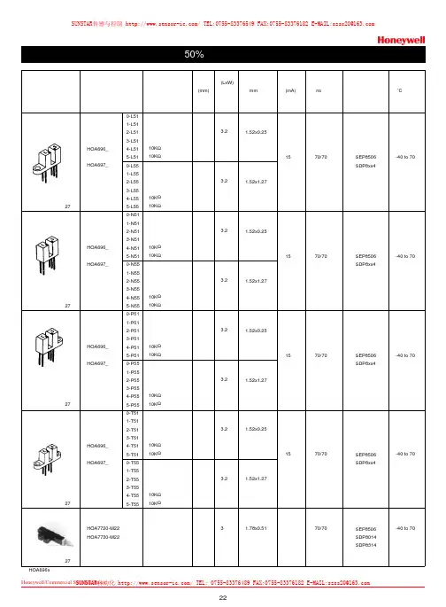
22Honeywell/Commercial Switch&Sensor 霍尼韦尔商业开关与传感器见27页见27页见27页见27页见27页型号HOA696_或HOA697_HOA696_或HOA697_HOA696_或HOA697_HOA696_或HOA697_HOA7720-M22HOA7730-M220-L511-L512-L513-L514-L515-L510-L551-L552-L553-L554-L555-L550-N511-N512-N513-N514-N515-N510-N551-N552-N553-N554-N555-N550-P511-P512-P513-P514-P515-P510-P551-P552-P553-P554-P555-P550-T511-T512-T513-T514-T515-T510-T551-T552-T553-T554-T555-T55输出 类型推挽 集电极开路 推挽 集电极开路10K Ω上拉电阻10K Ω上拉电阻 推挽 集电极开路 推挽 集电极开路10K Ω上拉电阻10K Ω上拉电阻 推挽 集电极开路 推挽 集电极开路10K Ω上拉电阻10K Ω上拉电阻 推挽 集电极开路 推挽 集电极开路10K Ω上拉电阻10K Ω上拉电阻 推挽 集电极开路 推挽 集电极开路10K Ω上拉电阻10K Ω上拉电阻 推挽 集电极开路 推挽 集电极开路10K Ω上拉电阻10K Ω上拉电阻 推挽 集电极开路 推挽 集电极开路10K Ω上拉电阻10K Ω上拉电阻 推挽 集电极开路 推挽 集电极开路10K Ω上拉电阻10K Ω上拉电阻推挽 集电极开路糟宽(LxW)3.23.23.23.23.23.23.23.23接受端 孔径 mm1.52x0.251.52x1.271.52x0.251.52x1.271.52x0.251.52x1.271.52x0.251.52x1.271.78x0.51最大触发电流(mA)15151515上升和下降时间 ns70/7070/7070/7070/7070/70内部收发 元件型号SEP8506SDP8xx4SEP8506SDP8xx4SEP8506SDP8xx4SEP8506SDP8xx4SEP8506SDP8014SDP8314工作温度范围 ˚C-40 to 70-40 to 70-40 to 70-40 to 70-40 to 70注:HOA696x 带有防尘的红外光可透过的滤光片,其余为不透光外壳,带小孔。
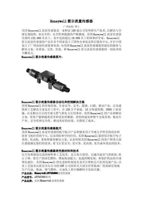
Honeywell霍尔流量传感器广州南创谭工美国Honeywell流量传感器是一家财富100强公司发明和生产技术,以解决与全球宏观趋势,如安全性,安全性和能源的严峻挑战。
美国Honeywell流量传感器全球约132,000名员工,其中包括超过19,000名工程师和科学家,Honeywell 霍尔流量传感器的产品在多个国家设立了国外办事处及售后服务中心,并在中国设立了广州南创传感器事业部,为美国Honeywell流量传感器提供最佳的服务与解决方案。
有质量,交货,价值,和Honeywell霍尔流量传感器做的一切技术的不懈重点。
Honeywell霍尔流量传感器图片:Honeywell霍尔流量传感器自动化和控制解决方案美国Honeywell的环境控制,生命安全,安全,遥感,扫描,移动产品,以及建筑和工艺解决方案是在工作中,在150万个家庭,10万座建筑物,5000工业设施,以及数以百计的全球天然气和电力公用事业。
美国Honeywell的产品和解决方案,使客户能够捕获更多和更好的数据,更快的速度和整个无线景观,提高生产率,安全性和安全性,推动更好的决策,并降低了成本。
Honeywell霍尔流量传感器航天美国Honeywell流量传感器的航空航天产品和服务用于全球几乎所有的商业和商务飞机经营的今天,以及国防和空间应用。
美国Honeywell提供综合航空电子系统,发动机,系统和服务解决方案,认真听取美国Honeywell的客户和重点放在最能满足他们的需求,使飞行更安全,更可靠,更高效,更具成本效益的技术。
Honeywell霍尔流量传感器高性能材料和技术以开发和制造先进的材料和工艺技术,是人每天使用,以减少温室气体排放,阻止子弹,使生产的绿色燃料,增加炼油能力,加速药物发现,和保护药品的全球领先地位。
美国Honeywell的先进材料制造尼龙至计算机芯片医药包装产品,以及工艺技术由霍尼韦尔公司的UOP公司的形式大部分世界炼油厂的基础有效地生产汽油,柴油,喷气燃料,石油化工和生物燃料开发的关键。
UC-8200SeriesArm Cortex-A7dual-core1GHz IIoT gateways with built-in LTE Cat.4,1mini PCIe expansion slot for a Wi-Fi module,1CAN port,4DIs,4DOsFeatures and Benefits•Armv7Cortex-A7dual-core1GHz•ISASecure IEC62443-4-2Security Level2certified with Moxa IndustrialLinux3Secure•Moxa Industrial Linux with10-year superior long-term support•LTE-ready computer with Verizon/AT&T certification and industrial-grade CE/FCC/UL certifications•Dual-SIM slots•2auto-sensing10/100/1000Mbps Ethernet ports•Integrated LTE Cat.4module with US/EU/APAC band support•1CAN port supports CAN2.0A/B•microSD socket for storage expansion•-40to85°C wide temperature range and-40to70°C with LTE enabledCertificationsIntroductionThe UC-8200computing platform is designed for embedded data acquisition applications.The computer comes with dual RS-232/422/485serial ports,dual10/100/1000Mbps Ethernet ports,and one CAN port as well as dual Mini PCIe socket to support Wi-Fi/cellular modules.These versatile capabilities let users efficiently adapt the UC-8200to a variety of complex communications solutions.The UC-8200is built around a Cortex-A7dual core processor that has been optimized for use in energy monitoring systems,but is widely applicable to a variety of industrial solutions.With flexible interfacing options,this tiny embedded computer is a reliable and secure gateway for data acquisition and processing at field sites as well as a useful communications platform for many other large-scale deployments.Wide temperature LTE-enabled models are available for extended temperature applications.All units are thoroughly tested in a testing chamber, guaranteeing that the LTE-enabled computing platforms are suitable for wide-temperature applications.AppearanceUC-8210UC-8220SpecificationsComputerCPU Armv7Cortex-A7dual-core1GHzDRAM2GB DDR3LSupported OS Moxa Industrial Linux1(Debian9,kernel4.4),2027EOLMoxa Industrial Linux31(Debian11,kernel5.10),2031EOLSee /MILStorage Pre-installed8GB eMMCExpansion Slots MicroSD(SD3.0)socket x13OS is selectable via Moxa Computer Configuration System(CCS)for CTO models.For the model names,see the Ordering Information section of thedatasheet PDF file.Computer InterfaceEthernet Ports Auto-sensing10/100/1000Mbps ports(RJ45connector)x2 Serial Ports RS-232/422/485ports x2,software selectable(DB9male) CAN Ports CAN2.0A/B x1(DB9male)Digital Input DIs x4Digital Output DOs x4USB2.0USB2.0hosts x1,type-A connectorsWi-Fi Antenna Connector UC-8220Models:RP-SMA x2Cellular Antenna Connector UC-8220Models:SMA x2GPS Antenna Connector UC-8220Models:SMA x1Expansion Slots UC-8220-T-LX:mPCIe slot x2UC-8220-T-LX US/EU/AP Models:mPCIe slot x1SIM Format UC-8220Models:NanoNumber of SIMs UC-8220Models:2Buttons Programmable buttonTPM TPM v2.0Ethernet InterfaceMagnetic Isolation Protection 1.5kV(built-in)Security FunctionsHardware-based Security TPM2.0Hardware Root of Trust Secure BootIntrusion Detection Host-based Intrusion DetectionSecurity Tools Security Diagnostic ToolSecurity Event AuditingSecure UpdateDisk Protection LUKS Disk EncryptionRecovery One-step recovery to the last known secure stateDual-system design with automatic failbackReliability Network Keep AliveNetwork Failover and FailbackSerial InterfaceBaudrate300bps to921.6kbpsData Bits7,8Stop Bits1,2Parity None,Even,Odd,Space,MarkFlow Control RTS/CTS,XON/XOFFADDC(automatic data direction control)for RS-485RTS Toggle(RS-232only)Console Port1x4-pin header to DB9console portRS-232TxD,RxD,RTS,CTS,DTR,DSR,DCD,GNDRS-422Tx+,Tx-,Rx+,Rx-,GNDRS-485-2w Data+,Data-,GNDCAN InterfaceNo.of Ports1Connector DB9maleBaudrate10to1000kbpsIndustrial Protocols CAN2.0ACAN2.0BIsolation2kV(built-in)Signals CAN_H,CAN_L,CAN_GND,CAN_SHLD,CAN_V+,GNDDigital InputsConnector Screw-fastened Euroblock terminalDry Contact Off:openOn:short to GNDIsolation3K VDCSensor Type Wet contact(NPN)Dry contactWet Contact(DI to COM)On:10to30VDCOff:0to3VDCDigital OutputsConnector Screw-fastened Euroblock terminalCurrent Rating200mA per channelI/O Type SinkVoltage24VDC nominal,open collector to30VDCCellular InterfaceCellular Standards LTE Cat.4Band Options US Models:LTE Band2(1900MHz)/LTE Band4(1700MHz)/LTE Band5(850MHz)/LTE Band13(700MHz)/LTE Band17(700MHz)UMTS/HSPA850MHz/1900MHzCarrier Approval:Verizon,AT&TEU Models:LTE Band1(2100MHz)/LTE Band3(1800MHz)/LTE Band5(850MHz)/LTE Band7(2600MHz)/LTE Band8(900MHz)/LTE Band20(800MHz)UMTS/HSPA850MHz/900MHz/1900MHz/2100MHzAP Models:LTE Band1(2100MHz)/LTE Band3(1800MHz)/LTE Band5(850MHz)/LTE Band7(2600MHz)/LTE Band8(900MHz)/LTE Band28(700MHz)UMTS/HSPA850MHz/900MHz/1900MHz/2100MHzReceiver Types GPS/GLONASS/GalileoState-of-the-art GNSS solutionAccuracy Position:2.0m@CEP50Acquisition Hot starts:1.1secCold starts:29.94secSensitivity Cold starts:-145dBmTracking:-160dBmTime Pulse0.25Hz to10MHzLED IndicatorsSystem Power x2Programmable x1SIM card indicator x1Wireless Signal Strength Cellular/Wi-Fi x6Power ParametersNo.of Power Inputs Redundant dual inputsInput Voltage12to48VDCPower Consumption10WInput Current0.8A@12VDCReliabilityAlert Tools External RTC(real-time clock)Automatic Reboot Trigger External WDT(watchdog timer)Physical CharacteristicsDimensions UC-8220Models:141.5x120x39mm(5.7x4.72x1.54in)UC-8210Models:141.5x120x27mm(5.7x4.72x1.06in)141.5x120x27mm(5.7x4.72x1.06in)Weight UC-8210Models:560g(1.23lb)UC-8220Models:750g(1.65lb)Housing SECCMetalIP Rating IP30Installation DIN-rail mountingWall mounting(with optional kit)Environmental LimitsOperating Temperature-40to70°C(-40to158°F)Storage Temperature(package included)-40to85°C(-40to185°F)Ambient Relative Humidity5to95%(non-condensing)Shock IEC60068-2-27Vibration2Grms@IEC60068-2-64,random wave,5-500Hz,1hr per axis(without USB devicesattached)Standards and CertificationsEMC EN55032/35EN61000-6-2/-6-4EMI CISPR32,FCC Part15B Class AEMS IEC61000-4-2ESD:Contact:4kV;Air:8kVIEC61000-4-3RS:80MHz to1GHz:10V/mIEC61000-4-4EFT:Power:2kV;Signal:1kVIEC61000-4-6CS:10VIEC61000-4-8PFMFIEC61000-4-5Surge:Power:0.5kV;Signal:1kV Industrial Cybersecurity IEC62443-4-1IEC62443-4-2Hazardous Locations Class I Division2ATEXIECExCarrier Approvals VerizonAT&TSafety UL62368-1EN62368-1Green Product RoHS,CRoHS,WEEEMTBFTime UC-8210-T-LX-S:708,581hrsUC-8220-T-LX:650,836hrsUC-8220-T-LX-US-S/EU-S/AP-S:528,574hrs Standards Telcordia(Bellcore)Standard TR/SRWarrantyWarranty Period5yearsDetails See /warrantyPackage ContentsDevice1x UC-8200Series computerDocumentation1x quick installation guide1x warranty cardInstallation Kit1x DIN-rail kit(preinstalled)1x power jack6x M2.5mounting screws for the cellular module Cable1x console cableDimensions UC-8210UC-8220Ordering Information12UC-8210-T-LX-SDefault:MIL1(-Debian9),2027EOLOrder WithModel UC-8210-T-LX-S(CTO):MIL3(Debian11)Secure/Standard,2031EOLWith MIL3Secure1GHzDual CoreBuilt in––-40to85°CUC-8220-T-LXDefault:MIL1(-Debian9),2027EOLOrder WithModel UC-8220-T-LX(CTO):MIL3(Debian11)Secure/Standard,2031EOLWith MIL3Secure1GHzDual CoreBuilt in Reserved Reserved-40to70°CUC-8220-T-LX-US-SDefault:MIL1(-Debian9),2027EOLOrder WithModel UC-8220-T-LX-US-S(CTO):MIL3(Debian11)Secure/Standard,2031EOLWith MIL3Secure1GHzDual CoreBuilt inUS region LTEmodulepreinstalledReserved-40to70°CUC-8220-T-LX-EU-SDefault:MIL1(-Debian9),2027EOLOrder WithModel UC-8220-T-LX-EU-S(CTO):MIL3(Debian11)Secure/Standard,2031EOLWith MIL3Secure1GHzDual CoreBuilt inEurope regionLTE modulepreinstalledReserved-40to70°CUC-8220-T-LX-AP-SDefault:MIL1(-Debian9),2027EOLOrder WithModel UC-8220-T-LX-AP-S(CTO):MIL3(Debian11)Secure/Standard,2031EOLWith MIL3Secure1GHzDual CoreBuilt inAPAC regionLTE modulepreinstalledReserved-40to70°CUC-8210-T-LX-S(CTO)MIL3(Debian11)Secure orStandard,2031EOLWith MIL3Secure1GHzDual CoreBuilt in––-40to85°CUC-8220-T-LX(CTO)MIL3(Debian11)Secure orStandard,2031EOLWith MIL3Secure1GHzDual Core–Reserved Reserved-40to70°CUC-8220-T-LX-US-S (CTO)MIL3(Debian11)Secure orStandard,2031EOLWith MIL3Secure1GHzDual CoreBuilt inUS region LTEmodulepreinstalledReserved-40to70°C12UC-8220-T-LX-EU-S (CTO)MIL3(Debian11)Secure orStandard,2031EOLWith MIL3Secure1GHzDual CoreBuilt inEurope regionLTE modulepreinstalledReserved-40to70°CUC-8220-T-LX-AP-S (CTO)MIL3(Debian11)Secure orStandard,2031EOLWith MIL3Secure1GHzDual CoreBuilt inAPAC regionLTE modulepreinstalledReserved-40to70°CAccessories(sold separately)Power AdaptersPWR-12150-EU-SA-T Locking barrel plug,12VDC,1.5A,100to240VAC,EU plug,-40to75°C operating temperature PWR-12150-UK-SA-T Locking barrel plug,12VDC,1.5A,100to240VAC,UK plug,-40to75°C operating temperature PWR-12150-USJP-SA-T Locking barrel plug,12VDC1.5A,100to240VAC,US/JP plug,-40to75°C operating temperature PWR-12150-AU-SA-T Locking barrel plug,12VDC,1.5A,100to240VAC,AU plug,-40to75°C operating temperature PWR-12150-CN-SA-T Locking barrel plug,12VDC,1.5A,100to240VAC,CN plug,-40to75°C operating temperature Power WiringCBL-PJTB-10Non-locking barrel plug to bare-wire cableCablesCBL-F9DPF1x4-BK-100Console cable with4-pin connector,1mWi-Fi Wireless ModulesUC-8200-WLAN22-AC Wireless package for UC-8200V2.0or later with Wi-Fi module,2screws,2spacers,1heat sink,1pad AntennasANT-LTEUS-ASM-01GSM/GPRS/EDGE/UMTS/HSPA/LTE,1dBi,omnidirectional rubber-duck antennaANT-LTE-ASM-04BK704to960/1710to2620MHz,LTE omnidirectional stick antenna,4.5dBiANT-LTE-OSM-03-3m BK700-2700MHz,multiband antenna,specifically designed for2G,3G,and4G applications,3m cable ANT-LTE-ASM-05BK704-960/1710-2620MHz,LTE stick antenna,5dBiANT-LTE-OSM-06-3m BK MIMO Multiband antenna with screw-fastened mounting option for700-2700/2400-2500/5150-5850MHzfrequenciesANT-WDB-ARM-02022dBi at2.4GHz or2dBi at5GHz,RP-SMA(male),dual-band,omnidirectional antennaDIN-Rail Mounting KitsUC-8210DIN-rail Mounting Kit DIN-rail mounting kit for UC-8210with4M3screwsUC-8220DIN-rail Mounting Kit DIN-rail mounting kit for UC-8220with4M3screwsWall-Mounting KitsUC-8200Wall-mounting Kit Wall-mounting kit for UC-8200with4M3screws©Moxa Inc.All rights reserved.Updated Jul18,2023.This document and any portion thereof may not be reproduced or used in any manner whatsoever without the express written permission of Moxa Inc.Product specifications subject to change without notice.Visit our website for the most up-to-date product information.。
T h e i n f o r m a t i o n p r o v i d e d i n t h i s d o c u m e n t a t i o n c o n t a i n s g e n e r a l d e s c r i p t i o n s a n d /o r t e c h n i c a l c h a r a c t e r i s t i c s o f t h e p e r f o r m a n c e o f t h e p r o d u c t s c o n t a i n e d h e r e i n .T h i s d o c u m e n t a t i o n i s n o t i n t e n d e d a s a s u b s t i t u t e f o r a n d i s n o t t o b e u s e d f o r d e t e r m i n i n g s u i t a b i l i t y o r r e l i a b i l i t y o f t h e s e p r o d u c t s f o r s p e c i f i c u s e r a p p l i c a t i o n s .I t i s t h e d u t y o f a n y s u c h u s e r o r i n t e g r a t o r t o p e r f o r m t h e a p p r o p r i a t e a n d c o m p l e t e r i s k a n a l y s i s , e v a l u a t i o n a n d t e s t i n g o f t h e p r o d u c t s w i t h r e s p e c t t o t h e r e l e v a n t s p e c i f i c a p p l i c a t i o n o r u s e t h e r e o f .N e i t h e r S c h n e i d e r E l e c t r i c I n d u s t r i e s S A S n o r a n y o f i t s a f f i l i a t e s o r s u b s i d i a r i e s s h a l l b e r e s p o n s i b l e o r l i a b l e f o r m i s u s e o f t h e i n f o r m a t i o n c o n t a i n e d h e r e i n .Product data sheetCharacteristicsMETSEPM2120EasyLogic PM2120, Power & Energy meter,up to the 15th harmonic, LED display, RS485,class 1MainRange EasyLogic Product name EasyLogic PM2100Device short name PM2120Product or component typePower meterComplementaryDevice application Sub billingPower monitoring Power quality analysis Total harmonic distortion Up to the 15th harmonicType of measurementApparent power min/max, totalActive and reactive power min/max, total Current min/max, avg Voltage min/max, avg Frequency min/max, avgTotal current harmonic distortion THD (I) per phase Total voltage harmonic distortion THD (U) per phase Power factor min/max, avg Apparent energy totalActive and reactive energy totalMetering typeCurrent I, I1, I2, I3Peak demand power PM, QM, SMActive, reactive, apparent energy (signed, four quadrant)Peak demand currents Active power P, P1, P2, P3Calculated neutral currentVoltage U, U21, U32, U13, V, V1, V2, V3Unbalance currentReactive power Q, Q1, Q2, Q3Demand power P, Q, SApparent power S, S1, S2, S3Accuracy classClass 1 active energy conforming to IEC 62053-21Class 1 reactive energy conforming to IEC 62053-24Class 5 harmonic distorsion (I THD & U THD)Measurement accuracyApparent power +/- 1 %Active energy +/- 1 %Reactive energy +/- 1 %Active power +/- 1 %Voltage +/- 0.5 %Power factor +/- 0.01Current +/- 0.5 %Frequency +/- 0.05 %Measurement current 5…6000 mAMeasurement voltage35…480 V AC 50/60 Hz between phases20…277 V AC 50/60 Hz between phase and neutral 480…999000 V AC 50/60 Hz with external VT Frequency measurement range 45…65 Hz[Us] rated supply voltage44...277 V AC 45...65 Hz +/- 10 %44...277 V DC +/- 10 %Network frequency50 Hz60 HzRide-through time100 Ms 120 V AC typical400 Ms 230 V AC typical50 ms 125 V DC typicalLine Rated Current1 A5 AMaximum power consumption in VA6 VA 277 V ACMaximum power consumption in W 3.3 W (power lines (AC))2 W at 277 V (power lines (DC))Input impedance Current (impedance <= 0.3 mOhm)Voltage (impedance > 5 MOhm)Tamperproof of settings Protected by access codeDisplay type7 segments LEDDisplay colour RedMessages display capacity 3 fields of 4 charactersDisplay digits12 - 0.56 in (14.2 mm)Demand intervals Configurable from 1 to 60 minInformation displayed Demand current (past value)Demand current (present value)Demand power (past value)Demand power (present value)VoltageCurrentFrequencyEnergy consumptionHarmonic distortionPower factorActive powerApparent powerReactive powerUnbalanced in %Control type 3 x buttonLocal signalling Red LED: output signal 1...9999000 pulse/ k_h (kWh, kVAh, kVARh)Green LED: module operation and integrated communicationNumber of inputs0Number of outputs0Communication port protocol Modbus RTU 4800 bps, 9600 bps, 19200 bps, 38.4 Kbps even/odd or none - 2wires 2500 VCommunication port support Screw terminal block: RS485Data recording Time stampingMin/max for 8 parametersFunction available Real time clockSampling rate64 samples/cycleCybersecurity Enable/disable communication portsCommunication service Remote monitoringProduct certifications CE IEC 61010-1CULus UL 61010-1CULus conforming to CSA C22.2 No 61010-1RCMEACC-TickMounting mode Clip-onMounting position VerticalMounting support FrameworkProvided equipment 1 x Installation guideMeasurement category Category III 480 VCategory II 480…600 VElectrical insulation class Double insulationClass IIFlame retardance V-0 conforming to UL 94Connections - terminals Current transformer screw connection bottom) 6Voltage inputs screw connection top) 4Material PolycarbonateWidth 3.78 in (96 mm)Depth Total 3.00 in (76.09 mm)Embedded 2.43 in (61.64 mm)Height 3.78 in (96 mm)Net Weight10.58 oz (300 g)Compatibility code PM2120EnvironmentService life7 year(s)IP degree of protection IP54 front: conforming to IEC 60529Body IP30 IEC 60529Relative humidity5…95 % 122 °F (50 °C)Pollution degree2Ambient air temperature for operation14…140 °F (-10…60 °C)Ambient air temperature for storage-13…158 °F (-25…70 °C)Operating altitude<= 6561.68 ft (2000 m)Electromagnetic compatibility Electrostatic discharge conforming to IEC 61000-4-2Radiated radio-frequency electromagnetic field immunity test IEC 61000-4-3Electrical fast transient/burst immunity test conforming to IEC 61000-4-4Surge immunity test IEC 61000-4-5Conducted RF disturbances conforming to IEC 61000-4-6Magnetic field at power frequency conforming to IEC 61000-4-8Voltage dips and interruptions immunity test IEC 61000-4-11Emission tests conforming to FCC part 15 class AOvervoltage category IIIOrdering and shipping detailsGTIN03606480800146Nbr. of units in pkg.1Package weight(Lbs)10.67 oz (302.5 g)Packing UnitsUnit Type of Package 1PCEPackage 1 Height 3.78 in (9.6 cm)Package 1 width 2.65 in (6.72 cm)Package 1 Length 4.00 in (10.16 cm)Unit Type of Package 2BB1Number of Units in Package 21Package 2 Weight14.25 oz (404 g)Package 2 Height 4.53 in (11.5 cm)Package 2 width 3.43 in (8.7 cm)Package 2 Length 4.72 in (12 cm)Unit Type of Package 3S03Number of Units in Package 318Package 3 Weight17.04 lb(US) (7.73 kg)Package 3 Height11.81 in (30 cm)Package 3 width11.81 in (30 cm)Package 3 Length15.75 in (40 cm)Offer SustainabilitySustainable offer status Green Premium productREACh Regulation REACh DeclarationEU RoHS Directive Compliant EU RoHS DeclarationMercury free YesRoHS exemption information YesChina RoHS Regulation China RoHS DeclarationEnvironmental Disclosure Product Environmental Profile Circularity Profile End Of Life Information。

3750This instruction sheet contains information about the Keithley Instruments Model Series 3700 Multifunction I/O Card connector pins, safety precautions, and product specifications.WARNING The following information is intended for qualified service personnel. Do not make module connections unless qualified to do so.To prevent electric shock that could result in serious injury or death, adhere to the followingsafety precautions:Before removing or installing a switch module in the mainframe, make sure the mainframe isturned off and disconnected from line power.Before making or breaking connections, make sure the power is removed from all externalcircuitry.Do not connect signals that may exceed the maximum specifications of the model orexternal wiring. Specifications for each circuit board are provided in the Series 3700 User'sManual.WARNING All wiring must be rated for the maximum voltage in the system. For example, if 300V is applied to the backplane connector, all module wiring must be rated for 300V.Information related to reading, writing, and controlling channels, as well as scanning, can be found in the Series 3700 System Switch/Multimeter User’s Manual. Detailed information about controlling the Series 3700 from a remote interface can be found in the Series 3700 System Switch/Multimeter Reference Manual.Four 32-bit counters are provided with a maximum input range of 1 MHz. Each counter has a gate input for control of event counting.Figure 1: Model 3750 Multifunction I/O CardDIGITAL I/O1Configuration: 40 bidirectional digital I/O bits arranged in 5 banks of 8 bits each. Each bank can be configured for either input or output capability. 1 bank of I/O is equivalent to 1 system channel.Digital Input specifications:An internal weak pull-up resistor of approximately 68 kΩ is provided on the card for each I/O. This pull-up resistor can be removed via onboard jumper on a channel (8 bit) basis. The pull-up voltage can either connect to the internally supplied 5V or an externally supplied voltage of up to 30V via onboard jumper. An internal 5V supply connection is separately available to run external logic circuits.Digital Input logic low voltage: 0.8V maxDigital Input logic high voltage: 2V min.Digital Input logic low current: -600uA max @ 0VDigital Input logic high current: 50uA max @ 5VLogic: Positive True.System Input Minimum Read speed2: 1000 readings / second.Maximum externally supplied pull-up voltage: 30V1 All channels power up configured as inputs.2 All channels configured as inputs.Digital Output logic high voltage: 2.4V minimum @ Iout = 10mA. sourcing only.Digital Output logic low voltage: 0.5V maximum @ Iout = -300mA sinking only.Maximum output sink current: 300mA per output, 3.0 A total per card.Logic: Positive True.System Output Minimum Write speed3: 1000 readings / second.Maximum externally supplied voltage to any digital I/O line: Pull-up voltage (5V internal or up to 30V external) Alarm: Trigger generation is supported for a maskable pattern match or state change on any of channels 1 through 5.Protection: Optional disconnect (set to inputs) during output fault conditions.Internal 5V logic supply: The internal logic supply is designed for powering external logic circuits of up to 50mA maximum. The logic supply is internally protected with a self-resetting fuse. Fuse reset time < 1 hour.3 All channels configured as outputs.32 - 1Input Signal Level: 200 mVp-p (minimum), 42V Peak (maximum)Threshold: AC (0V) or TTL Logic LevelGate Input: TTL-HI (Gate+), TTL-LO (Gate-) or NONE.Minimum Gate input setup time: 1usCount Reset: Manual or Read + ResetSystem Input Minimum Read speed: 1000 readings / second.Alarm: Trigger generation is supported for a count match or counter overflow on any of channels 6 though 9 ANALOG VOLTAGE OUTPUTThe isolated analog voltage output is designed for general purpose, low power applications.Output Amplitude4 ± 12V up to 10mAOverload Current: 21mA minimum.Resolution: 1mV.Full Scale Settling Time5: 1ms to 0.1% of output.DC Accuracy6: ± (% of output + mV)1 year 23 ± 5°C: 0.15% + 16mV90 day 23 ± 5°C: 0.1% + 16mV24 hour 23 ± 5°C: 0.04% + 16mVTemperature Coefficient: ± (0.02% + 1.2mV) / °C10mV Maximum Update Rate: 350us to 1% accuracy. System limited.Output Fault Detection: System fault detection is available for short circuit output / current compliance. Isolation: 300 V Peak Channel to Channel or Channel to Chassis.Protection: Optional disconnect during output fault conditions.4 Programming up to 1% over full scale range is supported5 Measured with standard load shown in Figure 16 Measured with > 10MΩ input DMM (DCV, filter, 1 PLC rate). Warm-up time is 1 hour @ 10mA load with 3750-STCompliance Voltage: 11V minimum.Maximum Open Circuit Voltage: 16VResolution: 1 uA.Full Scale Settling Time5: 1ms to 0.1% of output.DC Accuracy7: ± (% of output + uA)1 year 23 ± 5°C: 0.15% + 18uA90 day 23 ± 5°C: 0.1% + 18uA24 hour 23 ± 5°C: 0.04% + 18uATemperature Coefficient: ± (0.02% + 1.6uA) / °COutput Fault Detection: System fault detection is available for open circuit output / voltage compliance. Isolation: 300 V Peak Channel to Channel or Channel to Chassis.Protection: Optional disconnect during output fault conditions.CONNECTOR TYPE: Two 50 pin male D-shells.OPERATING ENVIRONMENT:Specified for 0ºC to 50ºC.Specified to 70% R.H. at 35ºCSTORAGE ENVIRONMENT: -25ºC to 65ºCWEIGHT: 1.27 kg (2.80 lb)FIRMWARE: Requires main revision to be 1.20 or above (Applies to all 3706 series mainframes) SAFETY: Conforms to European Union Directive 73/23/EEC, EN61010-1EMC: Conforms to European Union Directive 2004/108/EC, EN61326-1Power Budget Information:Quiescent Power: 3300 mWDigital Outputs each channel (1 through 5): 325 mWAnalog Channel each (10 & 11): 820 mW7 Measured with < 2Ω shunt DMM (DCI, filter, 1 PLC rate). Warm-up time is 1 hour with 3750-ST3790-KIT50-R 50 pin female D-sub connector kit (contains 2 female D-sub connectors and 100 solder-cups) 3721-MTC-3 50 pin D-sub female to male cable, 3m3721-MTC-1.5 50 pin D-sub female to male cable, 1.5m3750。
03s702IntroductionIn this document, we will discuss the specifications and features of the 03s702 model. This model is a versatile and high-performance device that is suitable for a wide range of applications. We will cover the technical specifications, key features, and potential uses for this product.Technical SpecificationsThe 03s702 model boasts impressive technical specifications that make it a powerful device. Here are some key specifications:•Processor: The device is powered by a high-performance quad-core processor, which ensures fast and efficient computing.•Memory: With 8GB of RAM, the device can easily handle multitasking and demanding applications.•Storage: The 03s702 model comes with a 512GB solid-state drive, providing ample space for storing files and data.•Display: The device features a 15.6-inch Full HD display, delivering crisp and vibrant visuals.•Battery Life: The built-in battery offers up to 8 hours of continuous usage, making it perfect for on-the-go use.•Operating System: It runs on the latest version of a popular operating system, ensuring a smooth and user-friendly experience.Key FeaturesThe 03s702 model comes packed with several key features that enhance its functionality and usability. Let’s take a closer look at some of these features:1.Ergonomic Design: The device sports a sleek and ergonomic design,making it comfortable to use for extended periods.2.High-Quality Audio: With built-in stereo speakers, the device deliversimmersive and clear sound quality.3.Connectivity Options: It offers a wide range of connectivity optionsincluding USB ports, HDMI, and Bluetooth, ensuring easy integration with other devices.4.Enhanced Security: The device features advanced security featuressuch as fingerprint recognition and facial recognition, providing additionalprotection for your data.5.Backlit Keyboard: The backlit keyboard allows for easy typing in lowlight conditions, improving productivity.6.Fast Charging: The device supports fast charging, allowing you toquickly charge the battery and minimize downtime.Potential UsesThe 03s702 model is a versatile device that can be used in various scenarios. Here are some potential uses for this product:1.Business Professionals: The device’s powerful performance and largestorage capacity make it ideal for business professionals who need to runresource-intensive applications and store large amounts of data.2.Students: The portable design and long battery life make it a greatchoice for students who need to work on assignments and projects on the go.3.Gamers: The high-quality display and powerful processor make itsuitable for gaming enthusiasts who want to enjoy an immersive gamingexperience.4.Content Creators: The device’s fast processing speed and amplestorage space make it perfect for content creators who need to edit videos,photos, or graphics.ConclusionThe 03s702 model is a feature-rich and high-performance device that offers a wide range of applications for different user groups. Its powerful specifications, key features, and potential uses make it a versatile and practical choice. Whether you are a business professional, student, gamer, or content creator, the 03s702 model has something to offer.。
HMT338 温湿度变送器用于压力管线维萨拉(Vaisala)HUMICAP® 温湿度变送器HMT330801价格变送器类型HMT3388探头电缆长度 2 米电缆,探头长度232mm V5 米电缆,探头长度232mm W10 米电缆,探头长度232mm X2 米电缆,探头长度454mm15 米电缆,探头长度454mm210 米电缆,探头长度454mm320 米电缆,探头长度454mm9无附加温度探头0测量参数RH+T ARH+T+Td+Tdf+a+x+Tw+ppm+pw+pws+h+dT B显示无0背光LCD图形显示1供电10...35 VDC, 24 VAC010...35 VDC, 24 VAC 带电源隔离 1普通AC供电 (100....240 VAC)2普通AC供电 (100....240 VAC),美国标准3普通AC供电 (100....240 VAC),欧洲标准4普通AC供电 (100....240 VAC),英国标准5普通AC供电(100....240 VAC) + 澳大利亚标准6外接美国适用的AC适配器(用于美国和加拿大的LAN/WLAN界面) 非IP659输出信号模拟输出通道(通道1,2 和3) 4... 20 mA1模拟输出通道(通道1,2 和3) 0... 20 mA2模拟输出通道(通道1,2 和3) 0... 1 V3模拟输出通道(通道1,2 和3) 0... 5 V4模拟输出通道(通道1,2 和3) 0... 10 V5*RS232串口界面或选择其它通讯模块模拟输出范围无第3模拟输出A通道1,2和3RH (0…100%RH)B B BT(温度范围见下表)C C CTd (-20…100ºC)D D DTdf (-20…100ºC) E E Ea (0…600g/m³) F F FTw (0…100ºC)G G Gx (0…500g/kg d.a)H H Hh (-40…1500kJ/kg)J J Jppm (0…5000)K K Kpw (0…100hPa)L L Lpws (0…100hPa)M M MdT (-10…+50ºC)N N N自定义自定参数/单位 Ch1:_____(___) Ch2:____(___) 选择 Ch3:_____(___)X X X自定量程 Ch1:_________ Ch2:_________ 选择 Ch3:___________通道1通道2通道3,如不需要,选择A模拟输出无温度输出A温度范围-40...+60°C B-40...+80°C C如果没有温度-40...+120°C D输出,请选择A-40...+180°C E-20...+60°C F-20...+80°C G-20...+120°C H-20...+180°C J0...+60°C K0...+100°C L0...+120°C M0...+180°C N-60...60 °C P自定义:_______________________X单位公制1非公制2模块插槽1选项无0继电器输出1RS-485数字串口,带隔离2LAN(以太网)接口+2米电缆(RJ45)4WLAN(无线以太网)接口+天线5数据记录模块6模块插槽2选项无0继电器输出1第3模拟输出选择第3通道模拟输出3数据记录模块如果模块插槽1已选数据记录模块,这无法在插槽2再选。
EasyLogic™PM2200系列用户手册NHA2778903-112022年5月法律声明施耐德电气品牌以及本指南中涉及的施耐德电气及其附属公司的任何商标均是施耐德电气或其附属公司的财产。
所有其他品牌均为其各自所有者的商标。
本指南及其内容受适用版权法保护,并且仅供参考使用。
未经施耐德电气事先书面许可,不得出于任何目的,以任何形式或方式(电子、机械、影印、录制或其他方式)复制或传播本指南的任何部分。
对于将本指南或其内容用作商业用途的行为,施耐德电气未授予任何权利或许可,但以“原样”为基础进行咨询的非独占个人许可除外。
施耐德电气的产品和设备应由合格人员进行安装、操作、保养和维护。
由于标准、规格和设计会不时更改,因此本指南中包含的信息可能会随时更改,恕不另行通知。
在适用法律允许的范围内,对于本资料信息内容中的任何错误或遗漏,或因使用此处包含的信息而导致或产生的后果,施耐德电气及其附属公司不会承担任何责任或义务。
EasyLogic™PM2200系列安全信息重要信息在尝试安装、操作、维修或维护本设备之前,请对照设备仔细阅读这些说明,以使自己熟悉该设备。
下列专用信息可能出现在本手册中的任何地方,或出现在设备上,用以警告潜在的危险或提醒注意那些对某过程进行阐述或简化的信息。
这两个符号中的任何一个与“危险”或“警告”安全标签一起使用,指示存在电击危险,若不遵循相关说明,可能会导致人身伤害。
这是安全警示符号。
它用来提醒您可能存在的人身伤害危险。
请遵守与此符号一起出现的全部安全信息,以避免可能的人身伤害或死亡。
危险危险表示存在危险情况,如果不避免,会导致死亡或严重人身伤害。
未按说明操作将导致人身伤亡等严重后果。
警告警告表示存在潜在的危险情况,如果不避免,可能导致死亡或严重人身伤害。
小心小心表示存在潜在的危险情况,如果不避免,可能导致轻微或中度人身伤害。
注意注意用于提醒注意与人身伤害无关的事项。
请注意电气设备应仅由经过认证的技术人员进行安装、操作、维护和维修。
替换机种特长替换内容●TOYOPUC-PC2●PC3JX/PC10GPC3JX:TCC-6901PC10G:TCC-6353・变更为PC3系列的支架、I/O模块、通信模块等预备品无需担心。
・在梯形回路中写入了注释可维护性提高注意事项・I/O模块输入输出点数由32点变更为16点。
I/O模块增加→安装空间不足 →2段式支架、平坦型等对应・I/O地址范围变为0~7FF(2048点)(PC3JX的I/O地址范围0~3FF(1024点)) →I/O地址不足时、使用PC10G通信模块●TOYOPUC-PC2J ●PC3JXPC3JX:TCC-6901・无需回路变更、能够使用既存模块・替换作业简单・在梯形回路中写入了注释可维护性提高・仅需更换CPU・其他 现行品能够流用・PC3JX无电池→无需定期更换通信模块●TOYOPUC-PC3J ●PC3JXPC3JX:TCC-6901・无需回路变更、能够使用既存模块・替换作业简单・仅需更换CPU・其他 现行品能够流用・PC3JX无电池→无需定期更换通信模块●TOYOPUC-PC3JD ●PC3JX-DPC3JX-D:TCC-6902IO328G:THK-6905・无需回路变更、能够使用既存模块・替换作业简单・仅需更换CPU・其他 现行品能够流用・PC3JX无电池→无需定期更换※CPU如有必要、按照以下所示替换通信模块●TOYOPUC-PC3JG(-P)●PC10GPC10G:TCC-6353IO328G:THK-6905IO329G:THK-6410DLNK-M2:THU-6099・无需回路变更、能够使用既存模块・替换作业简单・仅需更换CPU・其他 现行品能够流用※CPU如有必要、按照以下所示替换通信模块●TOYOPUC-M,M2●TOYOPUC-PC1※量产终了品、替换产品的详细信息请参照产品保守情报。
USB连接电缆推荐以下产品。
(2019年1月)※PLC更新时、扫描处理速度加快回路条件未满足场合、可以通过连续扫描功能进行改善。
CHAPTER 3 COST BEHAVIOR DISCUSSION QUESTIONS1. Knowledge of cost behavior allows a managerto assess changes in costs that result from changes in activity. This allows a manager to assess the effects of choices that change ac-tivity. For example, if excess capacity exists, bids that minimally cover variable costs may be totally appropriate. Knowing what costs are variable and what costs are fixed can helpa manager make better bids.2.The longer the time period, the more likelythat a cost will be variable. The short run is a period of time for which at least one cost is fixed. In the long run, all costs are variable. 3.Resource spending is the cost of acquiringthe capacity to perform an activity, whereas resource usage is the amount of activity actually used. It is possible to use less of the activity than what is supplied. Only the cost of the activity actually used should be assigned to products.4. Flexible resources are those acquired fromoutside sources and do not involve any long-term commitment for any given amount of re-source. Thus, the cost of these resources in-creases as the demand for them increases, and they are variable costs (varying in propor-tion to the associated activity driver).mitted resources are acquired by the useof either explicit or implicit contracts to obtaina given quantity of resources, regardless ofwhether the quantity of resources available is fully used or not. For multiperiod commit-ments, the cost of these resources essential-ly corresponds to committed fixed expenses.Other resources acquired in advance are short term in nature, and they essentially cor-respond to discretionary fixed expenses.6. A variable cost increases in direct proportionto changes in activity usage. A one-unit in-crease in activity usage produces an increase in cost. A step-variable cost, however, in-creases only as activity usagechanges in small blocks or chunks. An in-crease in cost requires an increase in severalunits of activity. When a step-variable costchanges over relatively narrow ranges of activ-ity, it may be more convenient to treat it as avariable cost.7.Mixed costs are usually reported in total inthe accounting records. The amount of thecost that is fixed and the amount that is vari-able are unknown and must be estimated. 8. A scattergraph allows a visual portrayal of therelationship between cost and activity. It re-veals to the investigator whether a relation-ship may exist and, if so, whether a linearfunction can be used to approximate the rela-tionship.9.Since the scatterplot method is not restrictedto the high and low points, it is possible toselect two points that better represent the re-lationship between activity and costs, produc-ing a better estimate of fixed and variablecosts. The main advantage of the high-lowmethod is the fact that it removes subjectivityfrom the choice process. The same line willbe produced by two different persons.10. Assuming that a scattergraph reveals that alinear cost function is suitable, then the me-thod of least squares selects a line that bestfits the data points. The method also providesa measure of goodness of fit so that thestrength of the relationship between cost andactivity can be assessed.11.The best-fitting line is the one that is “clo s est”to the data points. This is usually measuredby the line that has the smallest sum ofsquared deviations. No, the best-fitting linemay not explain much of the total cost varia-bility. There must be a strong relationship aswell.12.If the variation in cost is not well explained byactivity usage (coefficient of determination islow) as measured by a single driver, thenother explanatory variables may be needed inorder to build a good cost formula.13.The learning curve describes a situation inwhich the labor hours worked per unit de-crease as the volume produced increases.The rate of learning is determined empirically.In other words, managers use their know-ledge of previous similar situations to esti-mate a likely rate of learning.14.You would prefer a learning rate of 80 percentbecause that would lead to a faster decreasein the cumulative average time it takes to per-form the service. (To see this, rework Corner-stone 3-8 with an 85 percent learning rate.Note that the cumulative-average time for twosystems would be 850 hours rather than 800hours.)15.If the mixed costs are immaterial, then themethod of decomposition is unimportant. Fur-thermore, sometimes managerial judgmentmay be more useful for assigning costs thanthe use of formal statistical methodology.CORNERSTONE EXERCISESCornerstone Exercise 3.11. Total labor cost = Fixed labor cost + (Variable rate × Classes taught)= $600 + $20(Classes taught)2. Total variable labor cost = Variable rate × Classes taught= $20 × 100= $2,0003. Total labor cost = $600 + ($20 × Classes taught) = $600 + $2,000 = $2,6004. Unit labor cost = Total labor cost/Classes taught= $2,600/100= $265. New total classes = 100 + (0.50 × 100) = 150Total labor cost = $600 + ($20 × 150) = $3,600Unit labor cost = $3,600/150 = $24.00The unit labor cost went down because the fixed cost, which stays the same, is spread over a greater number of classes taught.Cornerstone Exercise 3.21. Activity rate = Total cost of purchasing agents/Number of purchase orders= (5 × $28,000)/(5 × 4,000)= $7.00/purchase order2. a. Total activity availability = 5 × 4,000 = 20,000 purchase ordersb. Unused capacity = 20,000 – 17,800 = 2,200 purchase orders3. a. Total activity availability = $7(5 × 4,000) = $140,000b. Unused capacity = $7(20,000 – 17,800) = $15,4004. Total activity availability = Activity capacity used + Unused capacity20,000 = 17,800 + 2,200or$140,000 = $124,600 + $15,4005. Four purchasing agents working full time and another working half time couldprocess 18,000 purchase orders (4.5 × 4,000). Since 17,800 purchase orders are processed, the unused capacity would be 200 purchase orders (18,000 –17,800).Cornerstone Exercise 3.31. Average workers’ salaries = $43,200/6 = $7,200Average temp agency payment = $6,240/6 = $1,040Average warehouse rental = $1,700/6 = $283 (rounded)Average electricity = $3,410/6 = $568 (rounded)Average depreciation = $13,200/6 = $2,200Average machine hours = 29,600/6 = 4,933 (rounded)Average number of orders = 1,720/6 = 287 (rounded)Average number of parts = 2,800/6 = 467 (rounded)2. Average fixed monthly cost = $7,200 + $2,200 = $9,400Variable rate for temp agency = $1,040/287 = $3.62 (rounded) per orderVariable rate for warehouse rental = $283/467 = $0.61 (rounded) per partVariable rate for electricity = $568/4,933 = $0.12 (rounded) per mach. hr.Monthly cost = $9,400 + $3.62(orders) + $0.61(parts) + $0.12(machine hours) 3. July cost = $9,400 + $3.62(420 orders) + $0.61(250 parts) + $0.12(5,900 mhrs.)= $9,400 + $1,520 + $153 + $708= $11,781 (rounded)4. New machine depreciation = ($24,000 – 0)/10 years = $2,400New machine depreciation per month = $2,400/12 = $200Only the fixed cost will be affected since depreciation is part of fixed cost.New fixed cost per month = $9,400 + $200 = $9,600New July cost = $9,600 + $1,520 + $153 + $708 = $11,981 (rounded)Cornerstone Exercise 3.41. Month with high number of purchase orders = AugustMonth with low number of purchase orders = February2. Variable rate = (High cost – Low cost)/(High purchase orders – Lowpurchase orders)= ($20,940 – $18,065)/(560 – 330) = $2,875/230= $12.50 per PO3. Fixed cost = Total cost – (Variable rate × Purchase orders)Let’s choose the high po int with cost of $20,940 and 560 purchase orders.Fixed cost = $20,940 – ($12.50 × 560)= $13,940(Hint: Check your work by computing fixed cost using the low point.)4. If the variable rate is $12.50 per purchase order and fixed cost is $13,940 permonth, then the formula for monthly purchasing cost is:Total purchasing cost = $13,940 + ($12.50 × Purchase orders)5. Purchasing cost = $13,940 + $12.50(430) = $19,3156. Purchasing cost for the year = 12($13,940) + $12.50(5,340)= $167,280 + $66,750 = $234,030The fixed cost for the year is 12 times the fixed cost for the month. Thus, instead of $13,940, the yearly fixed cost is $167,280.Cornerstone Exercise 3.51. Rounding the intercept to the nearest dollar, and the variable rate to the near-est cent, the formula for monthly purchasing cost is:Total purchasing cost = $15,021 + ($9.74 × Purchase orders)2. Purchasing cost = $15,021 + $9.74(430) = $19,209 (rounded)3. Purchasing cost for the year = 12($15,021) + $9.74(5,340)= $180,252 + $52,012 = $232,264 (rounded) The fixed cost for the year is 12 times the fixed cost for the month. Thus, instead of $15,021, the yearly fixed cost is $180,252 (rounded).Cornerstone Exercise 3.61. Degrees of freedom = Number of observations – Number of variables= 12 – 2 = 10The t-value from Exhibit 3-14 for 95 percent and 10 degrees of freedom is2.228.2. Predicted purchasing cost = $15,021 + ($9.74 × Purchase orders)= $15,021 + $9.74(430)= $19,209Confidence interval = Predicted cost ± (t-value × Standard error)= $19,209 ± (2.228 × $513.68)= $19,209 ± $1,144.48$18,065 ≤ Predicted value ≤ $20,3543. For a lower confidence level, the confidence interval will be smaller (narrower)since only a 90 percent degree of confidence is required. For a 90 percent confidence level with 10 degrees of freedom, the t-value is 1.812.Confidence interval = Predicted cost ± (t-value × Standard error)= $19,209 ± (1.812 × $513.68)= $19,209 ± $930.79$18,278 ≤ Predicted value ≤ $20,140Cornerstone Exercise 3.71. Rounding the regression estimates to the nearest cent, the formula formonthly purchasing cost is:Total purchasing cost = $14,460 + ($8.92 × Purchase orders) + ($20.39 × Non-standard orders)2. Purchasing cost = $14,460 + $8.92(430) + $20.39(45) = $19,213 (rounded)3. Purchasing cost for the year = 12($14,460) + $8.92(5,340) + $20.39(580)= $173,520 + $47,623.80 + $11,826.20= $232,979The fixed cost for the year is 12 times the fixed cost for the month. Thus, instead of $14,460, the yearly fixed cost is $173,520.Cornerstone Exercise 3.81. Cumulative Cumulative CumulativeNumber Average Time Total Time:of Units per Unit in Hours Labor Hours(column 1) (column 2) (3) = (1) × (2)1 500 5002 400 (0.80 × 500) 8004 320 (0.80 × 400) 1,2808 256 (0.80 × 320) 2,04816 204.8 (0.80 × 256) 3,276.8032 163.84 (0.80 × 204.80) 5,242.88Notice that every time the number of engines produced doubles, the cumula-tive average time per unit (in column 2) is just 80 percent of the previous amount.2. Cost for installing one engine = 500 hours × $30 = $15,000Cost for installing four engines = 1,280 hours × $30 = $38,400Cost for installing sixteen engines = 3,276.80 hours × $30 = $98,304Average cost per system for one engine = $15,000/1 = $15,000Average cost per system for four engines = $38,400/4 = $9,600Average cost per system for sixteen engines = $98,304/16 = $6,1443. Budgeted labor cost for experienced team = (5,242.88 – 3,276.80) × $30= $58,982 (rounded) Budgeted labor cost for new team = 3,276.80 × $30 = $98,304EXERCISESExercise 3.9Activity Cost Behavior Drivera. Vaccinating patients Variable Number of flu shotsb. Moving materials Mixed Number of movesc. Filing claims Variable Number of claimsd. Purchasing goods Mixed Number of orderse. Selling products Variable Number of circularsf. Maintaining equipment Mixed Maintenance hoursg. Sewing Variable Machine hoursh. Assembling Variable Units producedi. Selling goods Fixed Units soldj. Selling goods Variable Units soldk. Delivering orders Variable Mileagel. Storing goods Fixed Square feetm. Moving materials Fixed Number of moves n. X-raying patients Variable Number of X-rays o. Transporting clients Mixed Miles driven Exercise 3.101. Driver for overhead activity: Number of smokers2. Total overhead cost = $543,000 + $1.34(20,000) = $569,8003. Total fixed overhead cost = $543,0004. Total variable overhead cost = $1.34(20,000) = $26,8005. Unit cost = $569,800/20,000 = $28.49 per unit6. Unit fixed cost = $543,000/20,000 = $27.15 per unit7. Unit variable cost = $1.34 per unit8. a. and b. 19,500 Units 21,600 UnitsUnit cost a$29.19* $26.48Unit fixed cost b27.85* 25.14Unit variable cost c 1.34* 1.34a[$543,000 + $1.34(19,500)]/19,500; [$543,000 + $1.34(21,600)]/21,600b$543,000/19,500; $543,000/21,600c($29.19 – $27.85); ($26.48 – $25.14)*Rounded.Exercise 3.10(Concluded)The unit cost increases in the first case and decreases in the second. This is because fixed costs are spread over fewer units in the first case and over more units in the second. The unit variable cost stays constant.Exercise 3.111. a. Graph of equipment depreciation:Equipment Depreciation$0$5,000$10,000$15,000$20,00005,00010,00015,00020,00025,000Number of UnitsC o s tb. Graph of supervisors’ w ages:Supervisors' Wages$0$20,000$40,000$60,000$80,000$100,000$120,000$140,000$160,00005,00010,00015,00020,00025,000Number of UnitsC o stExercise 3.11 (Concluded)c. Graph of direct materials and power:Direct Materials and Power$0$20,000$40,000$60,000$80,000$100,00005,00010,00015,00020,00025,000Number of UnitsC o s t2. Equipment depreciation: FixedSupervisors’ wages: Fixed (A lthough if the step were small enough, the cost might be classified as variable —notice the cost follows a linear pattern; 5,000 units is a relatively wide step.) The normal operating range of the company falls entirely into the last step.Direct materials and power: VariableExercise 3.12Note: Resources acquired as needed are classified as short-term resources. The time horizon for as-needed resources, however, is much shorter than short term in advance resources (hours or days compared to months or a year).Exercise 3.131. Committed resources: Lab facility, equipment, and salaries of techniciansFlexible resources: Chemicals and supplies2. Depreciation on lab facility = $160,000/10 = $16,000Depreciation on equipment = $250,000/5 = $50,000Total salaries for technicians = 6 × $30,000 = $180,000Total water testing rate = ($16,000 + $50,000 + $180,000 + $50,000)/100,000= $2.96 per testVariable activity rate = $50,000/100,000 = $0.50 per testFixed activity rate = ($16,000 + $50,000 + $180,000)/100,000= $246,000/100,000= $2.46 per test3. Activity availability = Activity usage + Unused activityTest capacity available = Test capacity used + Unused test capacity100,000 tests = 86,000 tests + 14,000 tests4. Cost of activity supplied = Cost of activity used + Cost of unused activityCost of activity supplied = Cost of 86,000 tests + Cost of 14,000 tests [$246,000 + ($0.50 × 86,000)] = ($2.96 × 86,000) + ($2.46 × 14,000)$289,000 = $254,560 + $34,440Note: The analysis is restricted to resources acquired in advance of usage.Only this type of resource will ever have any unused capacity. (In this case, the capacity to perform 100,000 tests was acquired—facilities, people, and equipment—but only 86,000 tests were actually processed.)Exercise 3.141. a. Graph of direct labor cost:Direct Labor Cost$0$50,000$100,000$150,000$200,000$250,00001,0002,0003,0004,0005,000Units ProducedC o stb. Graph of cost of supervision:Cost of Supervision$0$20,000$40,000$60,000$80,000$100,000$120,000$140,00001,0002,0003,0004,0005,000Units ProducedC o s tExercise 3.14 (Concluded)2. Direct labor cost is a step-variable cost because of the small width of the step.The steps are small enough that we might be willing to view the resource as one acquired as needed and, thus, treated simply as a variable cost.Supervision is a step-fixed cost because of the large width of the step. This isa resource acquired in advance of usage, and since the step width is large,supervision would be treated as a fixed cost (discretionary—acquired in lum-py amounts).3. Currently, direct labor cost is $125,000 (in the 2,001 to 2,500 range). If produc-tion increases by 400 units next year, the company will need to hire one addi-tional direct laborer (the production range will be between 2,501 and 3,000), increasing direct labor cost by $25,000. This increase in activity will require the hiring of one new machinist. Supervision costs will remain the same as the increase in units does not require a new supervisor.Exercise 3.151. Supplies & Equipment Tanning NumberWages Maintenance Depreciation Electricity Minutes of Visits January $1,750 $1,450 $150 $ 300 4,100 410 February 1,670 1,900 150 410 3,890 380 March 1,800 4,120 150 680 6,710 560 Total $5,220 $7,470 $450 $1,390 14,700 1,350 ÷ 3 ÷ 3 ÷ 3 ÷ 3 ÷ 3 ÷ 3 Average $1,740 $2,490 $150 $ 463 4,900 450 2. Variable rate for supplies & maintenance = $2,490/450 = $5.53 per visitVariable rate for electricity = $463/4,900 = $0.09 per minuteFixed cost per month = $1,740 + $150 = $1,890Cost = $1,890 + $5.53(visit) + $0.09(minute)3. April cost = $1,890 + $5.53(360) + $0.09(3,700) = $4,214 (rounded)4. Monthly depreciation on new tanning bed = [($6,960 – 0)/4]/12 = $145New fixed cost = $1,890 + $145 = $2,035New April cost = $2,035 + $5.53(360) + $0.09(3,700) = $4,359 (rounded)Exercise 3.161. Variable rate for food and wages = $175,000/$560,000 = 0.3125 or 31.25% Variable rate for delivery costs = $18,000/8,000 = $2.25 per mile Variable rate for other costs = $9,520/14 = $680 per product 2. Total cost = $255,000 + 0.3125(sales) + $2.25(miles) + $680(product)3.The new menu offering will add $680 to monthly costs.Exercise 3.171. Scattergraph:Scattergraph of Radiology Tests$0$50,000$100,000$150,000$200,000$250,00001,0002,0003,0004,0005,000Number of TestsC o s tYes, there appears to be a linear relationship.Exercise 3.17 (Concluded)2. Low: 2,600, $135,060High: 4,100, $195,510V= (Y2–Y1)/(X2–X1)= ($195,510 – $135,060)/(4,100 – 2,600)= $60,450/1,500= $40.30 per testF= $195,510 – $40.30(4,100)= $30,280Y= $30,280 + $40.30X3. Y= $30,280 + $40.30(3,500)= $30,280 + $141,050= $171,330Exercise 3.181. Regression output from spreadsheet:SUMMA RY OUTPUTRegression StatisticsMultiple R 0.87621504R Square 0.7677528A djusted R Square 0.73457463Standard Error 11236.2148Observations 9A NOVAdf SS MS F Regression 1 2921521154 2.92E+09 23.1403 Residual 7 883767668 1.26E+08Total 8 3805288822Coefficients Standard Error t Stat P-value Intercept 36588.8206 28052.2996 1.304307 0.233375 X Variable 1 39.4759139 8.20630605 4.810436 0.001943Y = $36,588.82 + $39.48XExercise 3.18 (Concluded)2. Y= $36,588.82 + $39.48(3,500)= $36,588.82 + $138,180= $174,7693. R2 is about 0.73, meaning that about 73 percent of the variability in the radiol-ogy services cost is explained by the number of tests. The t statistic for X is4.81 and is significant, meaning that the number of tests is a good indepen-dent variable for radiology services. However, the t statistic for the intercept term is only 1.30, and is not significant. This, along with an R2 of only 73 per-cent, may mean that one or more other independent variables are missing. Exercise 3.191. Forklift depreciation:V= (Y2–Y1)/(X2–X1)= ($1,800 – $1,800)/(20,000 – 6,500) = $0F= Y2–VX2= $1,800 – $0(6,500) = $1,800Y= $1,800Indirect labor:V= (Y2–Y1)/(X2–X1)= ($135,000 – $74,250)/(20,000 – 6,500) = $4.50F= Y2–VX2= $74,250 – $4.50(6,500) = $45,000Y= $45,000 + $4.50XFuel and oil for forklift:V= (Y2–Y1)/(X2–X1)= ($15,200 – $4,940)/(20,000 – 6,500) = $0.76F= Y2–VX2= $15,200 – $0.76(20,000) = $0Y= $0.76XExercise 3.19 (Concluded)2. Forklift depreciation: Y= $1,800Indirect labor: Y= $45,000 + $4.50(9,000)= $85,500Fuel and oil for forklift: Y= $0.76(9,000)= $6,8403. Materials handling cost:= Forklift depreciation + Indirect labor + Fuel and oil for forklift= $1,800 + $45,000 + $4.50X + $0.76X= $46,800 + $5.26XFor 9,000 purchase orders:Y= $46,800 + $5.26X= $46,800 + $5.26(9,000)= $94,140Cost formulas can be combined if the activities they share have a common cost driver.Exercise 3.201. Y= $17,350 + $12X2. Y= $17,350 + $12(340)= $17,350 + $4,080= $21,430From Exhibit 3-14, the t-value for a 95 percent confidence level and degrees of freedom of 78, is 1.96. Thus, the confidence interval is computed as follows: Y f±t p S e$21,430 ± 1.96($220)$20,999 ≤Y f≤ $21,8613. To obtain the percentage explained, the correlation coefficient needs to besquared: 0.92 × 0.92 = 0.8464 or 84.64 percent. The standard error will produce an estimate within about $431 of the actual value with 95 percent confidence.The relationship is not bad, but might be improved by finding other explanato-ry variables. The unexplained variability (15 percent) may produce less accu-rate predictions.Exercise 3.211. Y= $1,980 + $2.56X1 + $67.40X2 + $2.20X3where Y= Total overhead costX1= Number of direct labor hoursX2= Number of wedding cakesX3= Number of gift baskets2. Y= $1,980 + $2.56(550) + $67.40(35) + $2.20(20)= $5,7913. The t-value for a 95 percent confidence interval and 20 (24 observations – 4variables) degrees of freedom is 2.086 (see Exhibit 3-14).Y f±t p S e$5,791 ± 2.086($65)$5,791 ±$136 (rounded to the nearest dollar)$5,655 ≤Y f≤ $5,9274. In this equation, the independent variables explain 92 percent of the variabilityin overhead costs. Overall, the equation is good. R2 is high; the t-values for all independent variables are quite high; and the confidence interval is relatively small giving Della a high degree of confidence that her actual overhead will fall into the range computed.Della can compare the additional cost of a gift basket ($2.20) to the price charged of $2.50. The cost is close to the price charged and does not seem excessive. If Della feels that the gift basket premium is high compared to what her competitors charge, she might look into less expensive sources of baskets, cellophane, and bows.Exercise 3.221. Y = $286,700 + $790X1– $45.50X2where Y= Total monthly cost of audit professional timeX1= Number of not-for-profit auditsX2= Number of hours of audit training2. Y= $286,700 + $790(9) – $45.50(130)= $287,895Exercise 3.22 (Concluded)3. The t-value for a 99 percent confidence interval and degrees of freedom of 19is 2.861 (see Exhibit 3-14).Y f±t p S e$287,895 ± 2.861($12,030)$287,895 ±$34,418 (rounded)$253,477 ≤Y f≤ $322,3134. The number of not-for-profit audits is positively correlated with audit profes-sional costs. Hours of audit training are negatively correlated with audit pro-fessional costs.5. In this equation, the independent variables explain 79 percent of the variabilityin audit costs. Overall, the equation is not bad. The confidence interval is rela-tively wide; however, the t-values are high, indicating that the independent va-riables chosen are predictors of audit costs. In addition, the signs on the independent variables are correct given Luisa’s experience with them. As long as the main reason for running the regression is to get some justification for audit training, the results are good. If Luisa wants to predict audit costs, however, she might try to find additional independent variables that would help explain more of the cost.Exercise 3.231. Cumulative Cumulative CumulativeNumber Average Time Total Time:of Units per Unit in Hours Labor Hours(column 1) (column 2) (3) = (1) × (2)1 600 6002 540 (0.90 × 600) 1,0804 486 (0.90 × 540) 1,9448 437.4 (0.90 × 486) 3,499.216 393.66 (0.90 × 437.4) 6,298.562. Cost for making one unit = 600 hours × $25 = $15,000Cost for making four units = 1,944 hours × $25 = $48,600Cost for making sixteen units = 6,298.56 hours × $25 = $157,464Average cost per unit for one unit = $15,000/1 = $15,000Average cost per unit for four units = $48,600/4 = $12,150Average cost per unit for sixteen units = $157,464/16 = $9,841.50Exercise 3.23 (Concluded)3. Cumulative Cumulative Cumulative TimeNumber Average Time Total Time: for Lastof Units per Unit in Hours Labor Hours Unit(column 1) (column 2) (1) × (2) (3) – (2)1 600 600 600.002 540 1,080 480.003 507.72 1,523.17 443.174 486 1,944 420.835 469.79 2,348.96 404.966 456.95 2,741.71 392.757 446.37 3,124.58 382.878 437.4 3,499.2 374.62Exercise 3.241. Cumulative Cumulative CumulativeNumber Average Time Total Time:of Units per Unit in Hours Labor Hours (column 1) (column 2) (3) = (1) × (2)1 1,000 1,0002 750 (0.75 × 1,000) 1,5004 562.5 (0. 75 × 750) 2,2508 421.88 (0.75 × 562.5) 3,37516 316.41 (0.75 × 421.88) 5,062.52. Total labor cost for eight sets = 3,375 hours × $40 = $135,000Total labor cost for sixteen sets = 5,062.5 hours × $40 = $202,5003. Cumulative Cumulative Cumulative TimeNumber Average Time Total Time: for Lastof Units per Unit in Hours Labor Hours Unit(column 1) (column 2) (1) × (2) (3) – (2)1 1,000 1,000 1,000.002 750 1,500 500.003 633.84 1,901.51 401.514 562.5 2,250 348.495 512.74 2,563.72 313.726 475.38 2,852.26 288.547 445.92 3,121.41 269.158 421.88 3,375 253.59Cost of eighth set = 253.59 hours × $40 = $10,143.60Exercise 3.251. f, kilowatt-hours2. a, sales revenues3. k, number of parts4. b, number of pairs5. g, number of credit hours6. c, number of credit hours7. e, number of nails8. d, number of orders9. h, number of gowns10. i, number of customers11. l, age of equipmentCPA-TYPE EXERCISESExercise 3.26d. Total contribution margin = Operating income + Fixed cost= $28,800 + $38,400 = $67,200 Number of units = Total contribution margin/unit contribution margin= $67,200/($18 − $12) = 11,200Exercise 3.27d.Exercise 3.28b. Total cost = 90(number of units) + 45= 90(100) + 45 = $9,000 + 45 = $9,045Exercise 3.29a.Exercise 3.30b. Total variable cost for Truck 415 = $0.13 × 125,000 miles = $16,250Cost per delivered pound = $16,250/(28,000 × 250) = $0.00232PROBLEMSProblem 3.311. Flexible resources: Direct materials, direct labor, machine operating costsCommitted resources—Long-term: MachiningCommitted resources—Short-term: Purchasing, inspection, and materialshandlingBoth short- and long-term committed resources are usually treated as fixed activity costs—discretionary fixed for short-term resources and committed fixed for long-term resources.2. Total annual resource spending:Activity Fixed Cost a Variable Cost b Total Cost Material usage —$ 75,000 $ 75,000Labor usage —25,000 25,000Machining $ 30,000 25,000 55,000Purchasing 100,000 —100,000Inspection 150,000 —150,000Materials handling 150,000 —150,000 Total $430,000 $125,000 $555,000a Machining: lease payment of $30,000Purchasing: 23,000 – 5,000 + 2,000 = 20,000, the required supply (demand).Since the resource is purchased in units of 5,000, the necessary supply can be reduced from 25,000 to 20,000. The cost of each block of resources is $25,000. Thus, resource spending is (20,000/5,000) × $25,000 = $100,000.Inspection: 9,000 + 750 = 9,750 as the demand. Since the resource is pur-chased in blocks of 2,000, the supply must equal 10,000. Thus, resource spending is (10,000/2,000) × $30,000 = $150,000.Materials handling: Demand = 4,300 + 500 – 200 = 4,600. Since the resource is purchased in blocks of 500, the required supply is 5,000. Thus, resource spending is (5,000/500) × $15,000 = $150,000.b Material usage: $0.75 × 100,000 = $75,000Labor usage: $0.25 × 100,000 = $25,000Machining: $0.50 × 50,000 = $25,000。