driver_controls

An Actual Driving LessonLearning to drive a manual carWhere are the controls that I might have to use in my driving:Knowing where the controls are, and being able to locate and use them without looking away from the road is important.Remember in each vehicle these controls could be in different places:-Washer and wiper, front and back-Head lights, high and low beam-Hand brake-Demisters, front and back-Horn-Hazard lights-IndicatorsHow to adjust the seat:When adjusting the seat in the car:The clutch pedal located on your left, should be depressed in to the floor and the seat adjusted so the left leg has a slight bend in it (about 15 degrees). The leg should not be fully extended.Push your shoulder into the back of the seat, and put your arms out in front of you at the top of the steering wheel, now adjust the back of the seat so your wrists are on top of the steering wheel rim (not your hand or arm but your wrist).Most cars now can adjust the height of the steering wheel. Move the steering wheel up or down so you can see the speedo clearly.How to adjust your mirrors:The mirrors should be adjusted so when you look into them, you are only moving your eyes not your head.The centre mirror:The top of your mirror should run along the top of your back window, you should be able to see the whole back window.The side mirrors:On a flat road, you should see road from the middle of the mirror to the bottom of the mirror, and from the middle of the mirror to the top of the mirror you should see houses, trees, sky etc.The bottom corner near the door of the mirror you should be able to see the back door handle.STAGE 1BUILDING A SOLID FOUNDATIONIn this part of learning you do it until you get it right. You will do lots of driving and hopefully turn action into habits, fix your mistakes. Repetition after repetition, do the same thing hundreds times of the correct repetition. (Sounds like fun doesn’t it).Learning the basic driving skillsDuring this stage the focus is on clutch control, gear changes, stopping and starting, acceleration and slowing down and steering (this is the frustrating stage of driving).Get the licensed driver to drive the car to a clear open road. We need a quiet road with few vehicles - a long straight road is perfect, no intersections.The safe way to get startedOnce a quiet road is found pull over to the side of the road, make the car safe (hand brake on, switch off the car). Change seats so the learner is in the driver’s seat and adjust the seat, mirror and steering wheel as demonstrated in that chapter.What are these pedals on the floor for?Look down at your feet - you will see three pedals. The one on the left is the clutch (in simple terms it basically transmits power from the engine to the wheels). Now that pedal is used by your left leg only - nothing else. The middle pedal is the brake (which stops or slows down the car). That pedal is used by the right leg only. The pedal on the right is the accelerator (which makes the car gather speed, or give it more power) that is also used by the right leg.The reason why the right leg is used by those pedals is that you are either braking or accelerating - you should not be doing both at the same time. (Stop or go). More important is that your legs hopefully will not get tangled up with each other, if that happens we will be in all sorts of trouble won’t we.Practise gear changes while the engine is off.While the engine is off let’s look at the gear stick and study how we are going to change gears, remember in each car it could be slightly different, your licensed driver will help. It is better to play with them while the engine is off (much safer I think).Practise going through the gears - first to second, second to third, third to fourth etc. Make sure you’ve got the clutch in when doing this. Keep practising until you can change all the gears without looking at them. Because when we are driving we should be looking at the road not the gear stick . When you are confident with that, then practise going down the gears. Up the gears, and down the gears.How to hold the gear stick?With your little finger to the top, and hand to the right side of the gear knob.1st to 2nd3rd back to 2nd2nd back to 1stThumb to the top and hand to the other side of the gear knob.2nd to 3rd gear3rd to 4th gear4th back to 3rd gearChanging up the gearsWhen we change gears we do so economically, we are not going for best performance (we are on public roads, not a speedway) this is all about safe driving. (Your licensed driver, I’m sure, would like to gethome safely after this practise.)Again different cars may be different but in most cars when changing up you would change gears about2000 to 2500 revs (most cars now will have a rev counter, a tachometer). At first keep a check with your gauge to tell you when to change gears, but eventually you will change gears by the sound of the engine without looking at the gauge.When going up the gears you always start in first and go through each gear.1st to 2nd ,2nd to 3rd,3rd to 4th etc. When changing gears get to the correct revs first, then accelerator offwith your right foot, then clutch in (it should go down quickly) with your left foot, change to the correctgear then clutch out, (the lower the gear used the slower the clutch pedal is released through thefriction point.) Then gently accelerate, one action at a time, but in a smooth flowing action. Pretend youare driving and practise speeding up and changing gears. To ease your stress make the car noise thatgoes with it. “vroom vroom”. When you feel comfortable practising changing up the gears, and also canchange up the gears without looking at the gear stick (we don’t want run off the road when we do it forreal) we will practise changing down the gears.The common errors to look out for when changing up. If you listen to and feel the car, the car will letyou know when something is not right. You just need to understand the car’s language.-Pushing down the clutch too soon before the accelerator is off. The car will rev up; the timing needs tobe right. (accelerator off then clutch in)- Changing up too soon. Make sure the revs are right, 2000 to 2500 rev. The engine will labour if the revsare too low for that gear. - Bringing the clutch out too fast. The car may jerk around a bit.-Accelerating too soon before the clutch is out after we selected the correct gear. (Clutch out than accelerate smoothly)Changing down the gears.When changing down the gears you can either go down each gear just like changing up the gears or youcan do the one shift change that is changing directly into the correct gear. e.g. 4th gear straight into 2ndgear. You simply do that by reaching the correct speed by braking then select the correct gear - it’s assimple as that. Some drivers like the feel of changing gears and prefer to change down each gear. But Imyself like to teach the one shift change to save wear and tear on my cars.Remember the brake and clutch have no direct link, you may still need to brake while you are already pressing the clutch in to change gears.To change down, brake to the correct speed and only then put your clutch in, change down into thecorrect gear then clutch out slowly. The lower the gear slower the clutch comes out. If you don’t changeat the correct speed you can do damage to the car. Again each car will be different but with most carsyou would change down as follows.4th to 3rd just below 50km3rd to 2nd just below 40km2nd to 1st just below 15kmThe common errors to look out for when changing down.-Not braking to the correct speed first. The car will over rev, this can cause damage. -Clutch coming out too fast. The car will jerk around a bit.-Selecting the wrong gear. The car will rev up or labour. -Accelerating before the clutch is out. The car will rev up.Starting the car, in a manual car.Make sure you follow this procedure or else the car will more likely to take off without warning. Wedon’t want any mishaps yet because at this stage we are doing well.–Press the clutch in (left pedal) with the left leg and hold it down.-Make sure the handbrake is fully on.Anytime you put your hand brake on always make sure it is fully on, not just partly on. The car may stillroll if it is not.-Move the gear stick to neutralThis is the middle position that feels free when moving it from side to side the car is now considered“out of gear”.- Start the engine with the key, by turning the key to the right and when the engine revs up let thekey go it will automatically spring back; during all of this remember you still got your clutch fully down.“Congratulations you have now started the car”.Make sure the gear stick is still in neutral and hand brake is on; you can now release the clutch and relax for a minute or two. The car should be idling along (there is no hurry).“Let’s get the car movi ng shall we”.Clutch control is easy to achieve, if you use the right technique and work at it. Some learners may take longer than others to get good clutch control.I’ve found at this stage, students will pick up good clutch control much quicker if we start off without using the accelerator to get the car moving. We are getting to know the feel of the clutch. Most cars you should be able to do this but if your car won’t allow this, this is fine also, you will skip this part and pick up again we start using the accelerator.First thing we have to identify what’s called the friction point of the clutch. This is the point when the clutch starts to meet, you can tell by the engine will just start to lose revs, and you should able to feel the car wanting to go forward. This is the first stage we have to master. When the clutch is fully down to the floor and to the friction point nothing will happen, it’s when you go through the friction point that’s when things will happen. Now remember at this stage we are not getting the car moving, if the car moves then the clutch has come out too far.-Press the clutch down fully to the floor.-Make sure the hand brake is off.-Move the gear stick to 1st gear. (The car is now in gear)-Slowly, at this stage very slowly lift foot up from the clutch until you hear the engine revs begin to drop, you can also watch the rev counter if you like that will start to drop also. And hold the clutch still. Remember, we are not moving the car at this stage, if the car has moved the clutch is out to far. We are only finding the friction point.-Clutch back in and relax-Keep doing this until you can go straight to that point fairly quickly. You may only have to do it a few times or you may have to do it a hundred times it doesn’t matter. Th e main thing you have master finding the friction point. You should instantly recognize the sound of the engine and the feel of the clutch. When you feel confident relax for few minute because the next stage all the works begin. Clutch fully in than slowly bring it out until you feel the clutch starts to take.Now I said this is the most frustrating part of learning to drive; you are going to find out why I said that. Have you got composure again?We have learnt about the friction of the clutch now we talk about the engagement part of the clutch. That is when the clutch pedal is between the friction point and until it is fully out. This is the hardest part to master. When you feel comfortable with this part we are nearly there.Two common errors may occur.-You will bring the clutch out slow, but when you feel the car starts to move automatically you will want to move your clutch out quickly. NOOOOOO!If you do that that the car will go mad and jump around on you and then stall the engine. As soon as you feel that, immediately put your clutch back in.-The next error is you will bring your clutch out about 80% of the way slowly and then automatically you want to bring you clutch out quickly. NOOOOO!If you do that that you will feel a big kick in the car. We want a smooth take off.Now we know what things might happen we will try to avoid them. O.K.Let’s do it for real. Remember, we are only working the clutch, nothing else.Get to the friction point as fast as you like, hold the clutch pedal steady, feel the car moving slowly as you bring the pedal through the engagement of the clutch. You are moving the clutch a centimetre at a time. If the car stalls, slow the clutch down even slower next time. You need to feel the car moving as you take off. Keep doing this until you are happy with yourself.As soon as you feel the friction point slow the clutch down until you are fully out. Between the friction points and fully out should take about two seconds.When merging into traffic we will have to move the car faster than that or we are never merging into traffic. So how do we merge into traffic? The car needs extra power - as simple as that.Just imagine you’ve got a wheelbarrow full of something heavy (bricks or dirt) - to get the wheelbarrow moving you have to strengthen your muscles up, and give it a big push and when it’s moving it becomes easier doesn’t it, you’ve got your momentum going. Same thing with a car. To get the bulk and weight of the car moving it needs extra power; you do that by giving it more accelerator. Makes sense.Let’s take off without the accelerator again, I want to demonstrate something. Bring your clutch to the friction point; now look at your rev counter see what happens when going through the engagement point, the rev counter is droppi ng, right? It’s using up extra power to get the car moving, that’s when you need to give it more accelerator to keep the power up to it or else it will stall and then you can take off quicker without stalling the car. Believe me this is the hardest part to master.Common errors to look out forToo much accelerator, the car will over rev. That’s not good for the engine.Not enough revs. The car will stall. That’s embarrassing.The clutch comes out too fast, the car will stall.Let’s do this now.-Get the friction point.-Bring the rev counter to about 2,000 revs.-Bring the clutch fully out at the same time keep the rev up to about 2,000 revs with your accelerator. For the first time the clutch and the accelerator works together. This is hard tomaster.-Clutch back in.-Repeat, repeat, repeat as much as it takes to get it right.You may have to practise that a lot of times before you become comfortable with it.When you feel comfortable lets go for a drive. Put all our work together that we have practised. Start, stop, up the gears, down the gears. Let’s go over it once more.-Clutch in.-1st gear.-Hand brake off.-Get the friction point of the clutch.-Revs up to 2000.-Bring the clutch out slowly, keeping the revs up.-When clutch is fully out and at 2,500 rev change into second gear (remember how to hold the gear stick)-Clutch out, than accelerate-Repeat until we have gone through the gears.Now imagine going down the gears. Make sure you are at the right speed before putting the clutch in to change down. You should feel confident now, even though we have only done it in our mind.We are really doing it for real for the first(Watch out everybody I’m coming)-Clutch in.-1st gear-Handbrake off.-Bring clutch to friction point.-Check to see if it is safe to merge onto the road (if not wait until it is)-Revs to 2,000 revs-Clutch out slowly keeping the revs upIf things feel wrong clutch in quickly and start again.-Clutch fully out.-Keeping light on the accelerator bring the revs up to 2,500 revs.-Accelerator off.-Clutch in.-Holding the gear stick correctly change into 2nd gear.-Clutch out slowly.If this was not smooth more likely the clutch came out too quickly-Accelerate to 2,500 revs.-At 2,500revs accelerator off.-Clutch in.-Holding the gear stick correctly change to 3rd gear.-Clutch out slowly.-Accelerate to 2,500 revs.-At 2,500 revs accelerator off.-Clutch in.-Holding the gear stick correctly change into 4th gear.-Clutch out.We did it for the first time yippee!!!!!!!Calm down! Remember we’re driving on the road. Keep our concentration on the road shall we.Let’s pull over to the side of the road and start again.-Check your mirrors for cars behind you.-Indicate to let other vehicles know what we are doing.-Brake smoothly and gently.-When the car slows down to about 40km/h gently move off the road.We need the get the speed off the car first before moving off the road.-Clutch in. (Because we are coming to a stop no need to change down the gears)-Bring the car to a stop (keep your clutch in)-Select neutral.-Hand brake on.-Now release your clutch and relax a bit.When you are ready let’s practice going down the gears.Let’s go, show me how you go up the gears, but this time no help from me.“Well done”Now we’re driving on the road let’s go down the gears, make sure before we do this there are no other vehicles around. Only do it if it’s safe.-Accelerator off.-Brake to about 50km/h.-Clutch in.-Holding the gear stick correctly change into 3rd gear.-Clutch out slowly.Lower the gear, slower the clutch comes out.-Brake to about 40km/h-Holding the gear stick correctly change into 2nd gear.-Clutch out slowly.Now accelerate and go up the gears.Keep on doing this, up the gears, down the gears, up the gears, down the gears.Stopping the car where we need it to stop.While we are on the quiet road let’s practise stopping the car where we need the car to stop.Just imagine we are coming to an intersection with a stop sign. The object is to stop the car close as possible to the stop line without going over the stop line. If we can’t do that we are in big trouble, so let’s practise this where there are no cars around. What I do is to have an imaginary white line across the road, or better still look at the white guide posts along the side of the road - have an imaginary white line between the white posts. What we’ve got to do is the stop the car as close possible, at least within 1metre of the imaginary line without going over. Can you see why I said start off in the quietest road youcan find?We need to have a smooth stop. Not brake-accelerate-brake situation. Do the bulk of your braking first, than release the pressure on the brake pedals as you get closer. It should feel like you are rolling in. Youare only releasing the pressure on the brake, not releasing it fully - if you do that the car will gather speed. It takes practice to know how much pressure to put on the brake pedal and how much pressure to release from the brake pedals.Common errors to look out for.Braking too hard, if you do that than you will stop short of your line and you will have to accelerateagain to reach the correct position.Braking too soft, if you do that you will have to brake harder at the end or you finish up in the intersection. That’s dangerous. This will be unpleasant for the passengers and dangerous. Clutch coasting, that’s putting your clutch in too soon, letting the car roll for too long, this may cost you demerit points in the driving test. Forgetting to put your clutchin or putting it in too late. This will cause the car to stall or make the engine labour. We need a smooth stop. Let’s do it. When it’s safe we will drive off following all the procedures we have learnt.Right, when you are ready :-Have an imaginary line across the road, well ahead of you. Or a tree, or something.-Start to brake-As you get closer to your imaginary line apply more pressure on the brake. If you have misjudged the distance you’re coming in too fast.Or release the pressure on your brake pedal if you are going to stop short of your imaginary line.We are only working the pressure on the brake pedal not fully releasing the brake pedal, or elsethe car will gather speed again.-Clutch pedal fully in about ten metres before the line.-Bring the car to a stop within 1 metre of that imaginary line but not over it.-Drive off again.-Repeat, repeat, repeat until you have it right and you are happy with yourself.Clutch control.Sometimes going as fast as the idling speed is too fast. What I mean by that is moving in 1st gear without any accelerator is sometimes too fast e.g. doing a parallel reverse park, reversing out of an angle park or driving in heavy traffic. In these situations we need to ride the clutch to make the car go slower. Keep thisto the minimum because i t’s wearing away your clutch faster, but sometimes we have to do this tocontrol the car.Basically your clutch pedal becomes the accelerator and the accelerator pedal is just to keep the revs upso you do not stall or labour the engine. This how we do it-Remember the friction point of the clutch, hold your clutch there-You may need a little accelerator to keep up the revs.-Very slowly adjust your clutch pedal to match the speed you need and hold your clutch pedal there.The more you bring your clutch pedal out the faster the car will go, that is what I meant when I said the clutch will become your accelerator. This will take some practise.___________________________________________________________________________How’s that. Hopefully you will able to take control of your driving. This is the most dangerous part of your driving because you need to stop and start a lot. Always make sure it’s safe before you do something.I wish you good luck and safe driving. We still have a long way to go yet. Basic car control may take up to 15 to 20 hours of experience before you are ready for the next stage. At this stage it’s only open road driving. Everyone learns at a different pace. Driving instructors can push you a little bit harder because they should have dual controls in their car - you don’t. The next stage will be light traffic driving in residential streets.。

Legal informationCopyright and License© Copyright 2019 HP Development Company, L.P.Reproduction, adaptation, or translation without prior written permission is prohibited, except as allowedunder the copyright laws.The information contained herein is subject to change without notice.The only warranties for HP products and services are set forth in the express warranty statementsaccompanying such products and services. Nothing herein should be construed as constituting anadditional warranty. HP shall not be liable for technical or editorial errors or omissions contained herein.Edition 1, 10/2019Trademark CreditsAdobe®, Adobe Photoshop®, Acrobat®, and PostScript® are trademarks of Adobe Systems Incorporated.Apple and the Apple logo are trademarks of Apple Inc., registered in the U.S. and other countries.macOS is a trademark of Apple Inc., registered in the U.S. and other countries.AirPrint is a trademark of Apple Inc., registered in the U.S. and other countries.Google™ is a trademark of Google Inc.Microsoft®, Windows®, Windows® XP, and Windows Vista® are U.S. registered trademarks of MicrosoftCorporation.UNIX® is a registered trademark of The Open Group.iiiT able of contents1 Printer overview (1)Warning icons (1)Potential shock hazard (2)Printer views (2)Printer front view (2)Printer back view (4)Interface ports (4)Control-panel view (5)How to use the touchscreen control panel (7)Printer specifications (8)T echnical specifications (8)Supported operating systems (11)Mobile printing solutions (12)Printer dimensions (13)Power consumption, electrical specifications, and acoustic emissions (15)Operating-environment range (15)Printer hardware setup and software installation (16)2 Paper trays (17)Introduction (17)Load paper to Tray 1 (multipurpose tray) (17)Load Tray 1 (multipurpose tray) (18)Tray 1 paper orientation (19)Use alternative letterhead mode (24)Enable Alternative Letterhead Mode by using the printer control-panel menus (24)Load paper to Tray 2 (24)Load Tray 2 (24)Tray 2 paper orientation (26)Use alternative letterhead mode (29)Enable Alternative Letterhead Mode by using the printer control-panel menus (29)Load paper to the 550-sheet paper tray (30)Load paper to the 550-sheet paper tray (30)550-sheet paper tray paper orientation (32)Use alternative letterhead mode (35)Enable Alternative Letterhead Mode by using the printer control-panel menus (35)ivLoad paper to the 2 x 550-sheet paper trays (36)Load paper to the 2 x 550-sheet paper trays (36)2 x 550-sheet paper tray paper orientation (38)Use alternative letterhead mode (41)Enable Alternative Letterhead Mode by using the printer control-panel menus (41)Load paper to the 2,700-sheet high-capacity input paper trays (41)Load paper to the 2,700-sheet high-capacity input paper trays (41)2,700-sheet HCI paper tray paper orientation (43)Use alternative letterhead mode (45)Enable Alternative Letterhead Mode by using the printer control-panel menus (45)Load and print envelopes (46)Print envelopes (46)Envelope orientation (46)Load and print labels (47)Manually feed labels (47)Label orientation (48)3 Supplies, accessories, and parts (49)Order supplies, accessories, and parts (49)Ordering (49)Supplies and accessories (50)Maintenance/long-life consumables (51)Customer self-repair parts (51)Dynamic security (52)Configure the HP toner-cartridge-protection supply settings (53)Introduction (53)Enable or disable the Cartridge Policy feature (53)Use the printer control panel to enable the Cartridge Policy feature (54)Use the printer control panel to disable the Cartridge Policy feature (54)Use the HP Embedded Web Server (EWS) to enable the Cartridge Policy feature (54)Use the HP Embedded Web Server (EWS) to disable the Cartridge Policy feature (55)Troubleshoot Cartridge Policy control panel error messages (55)Enable or disable the Cartridge Protection feature (55)Use the printer control panel to enable the Cartridge Protection feature (56)Use the printer control panel to disable the Cartridge Protection feature (56)Use the HP Embedded Web Server (EWS) to enable the Cartridge Protection feature (56)Use the HP Embedded Web Server (EWS) to disable the Cartridge Protection feature (57)Troubleshoot Cartridge Protection control panel error messages (57)Replace the toner cartridges (58)T oner-cartridge information (58)Remove and replace the cartridges (59)Replace the imaging drums (62)Imaging drum information (62)Remove and replace the imaging drums (63)Replace the toner-collection unit (66)T oner-collection unit information (66)vRemove and replace the toner-collection unit (67)Replace the staple cartridge (M776zs model only) (70)Staple cartridge information (70)Remove and replace the staple cartridge (71)4 Print (73)Print tasks (Windows) (73)How to print (Windows) (73)Automatically print on both sides (Windows) (74)Manually print on both sides (Windows) (74)Print multiple pages per sheet (Windows) (75)Select the paper type (Windows) (75)Additional print tasks (76)Print tasks (macOS) (77)How to print (macOS) (77)Automatically print on both sides (macOS) (77)Manually print on both sides (macOS) (77)Print multiple pages per sheet (macOS) (78)Select the paper type (macOS) (78)Additional print tasks (79)Store print jobs on the printer to print later or print privately (79)Introduction (79)Create a stored job (Windows) (79)Create a stored job (macOS) (80)Print a stored job (81)Delete a stored job (81)Delete a job that is stored on the printer (81)Change the job storage limit (82)Information sent to printer for Job Accounting purposes (82)Mobile printing (82)Introduction (82)Wi-Fi, Wi-Fi Direct Print, NFC, and BLE printing (82)Enable wireless printing (83)Change the Wi-Fi Direct name (83)HP ePrint via email (83)AirPrint (84)Android embedded printing (85)Print from a USB flash drive (85)Enable the USB port for printing (85)Method one: Enable the USB port from the printer control panel (85)Method two: Enable the USB port from the HP Embedded Web Server (network-connectedprinters only) (85)Print USB documents (86)Print using high-speed USB 2.0 port (wired) (86)Method one: Enable the high-speed USB 2.0 port from the printer control panel menus (86)Method two: Enable the high-speed USB 2.0 port from the HP Embedded Web Server (network-connected printers only) (87)vi5 Copy (88)Make a copy (88)Copy on both sides (duplex) (90)Additional copy tasks (92)6 Scan (93)Set up Scan to Email (93)Introduction (93)Before you begin (93)Step one: Access the HP Embedded Web Server (EWS) (94)Step two: Configure the Network Identification settings (95)Step three: Configure the Send to Email feature (96)Method one: Basic configuration using the Email Setup Wizard (96)Method two: Advanced configuration using the Email Setup (100)Step four: Configure the Quick Sets (optional) (104)Step five: Set up Send to Email to use Office 365 Outlook (optional) (105)Introduction (105)Configure the outgoing email server (SMTP) to send an email from an Office 365 Outlookaccount (105)Set up Scan to Network Folder (108)Introduction (108)Before you begin (108)Step one: Access the HP Embedded Web Server (EWS) (108)Step two: Set up Scan to Network Folder (109)Method one: Use the Scan to Network Folder Wizard (109)Method two: Use Scan to Network Folder Setup (110)Step one: Begin the configuration (110)Step two: Configure the Scan to Network Folder settings (111)Step three: Complete the configuration (118)Set up Scan to SharePoint (118)Introduction (118)Before you begin (118)Step one: Access the HP Embedded Web Server (EWS) (118)Step two: Enable Scan to SharePoint and create a Scan to SharePoint Quick Set (119)Scan a file directly to a SharePoint site (121)Quick Set scan settings and options for Scan to SharePoint (122)Set up Scan to USB Drive (123)Introduction (124)Step one: Access the HP Embedded Web Server (EWS) (124)Step two: Enable Scan to USB Drive (124)Step three: Configure the Quick Sets (optional) (125)Default scan settings for Scan to USB Drive setup (126)Default file settings for Save to USB setup (126)Scan to email (127)Introduction (127)Scan to email (127)Scan to job storage (129)viiIntroduction (129)Scan to job storage on the printer (130)Print from job storage on the printer (132)Scan to network folder (132)Introduction (132)Scan to network folder (132)Scan to SharePoint (134)Introduction (134)Scan to SharePoint (134)Scan to USB drive (136)Introduction (136)Scan to USB drive (136)Use HP JetAdvantage business solutions (138)Additional scan tasks (138)7 Fax (140)Set up fax (140)Introduction (140)Set up fax by using the printer control panel (140)Change fax configurations (141)Fax dialing settings (141)General fax send settings (142)Fax receive settings (143)Send a fax (144)Additional fax tasks (146)8 Manage the printer (147)Advanced configuration with the HP Embedded Web Server (EWS) (147)Introduction (147)How to access the HP Embedded Web Server (EWS) (148)HP Embedded Web Server features (149)Information tab (149)General tab (149)Copy/Print tab (150)Scan/Digital Send tab (151)Fax tab (152)Supplies tab (153)Troubleshooting tab (153)Security tab (153)HP Web Services tab (154)Networking tab (154)Other Links list (156)Configure IP network settings (157)Printer sharing disclaimer (157)View or change network settings (157)Rename the printer on a network (157)viiiManually configure IPv4 TCP/IP parameters from the control panel (158)Manually configure IPv6 TCP/IP parameters from the control panel (158)Link speed and duplex settings (159)Printer security features (160)Introduction (160)Security statements (160)Assign an administrator password (160)Use the HP Embedded Web Server (EWS) to set the password (160)Provide user access credentials at the printer control panel (161)IP Security (161)Encryption support: HP High Performance Secure Hard Disks (161)Lock the formatter (161)Energy-conservation settings (161)Set the sleep timer and configure the printer to use 1 watt or less of power (161)Set the sleep schedule (162)Set the idle settings (162)HP Web Jetadmin (163)Software and firmware updates (163)9 Solve problems (164)Customer support (164)Control panel help system (165)Reset factory settings (165)Introduction (165)Method one: Reset factory settings from the printer control panel (165)Method two: Reset factory settings from the HP Embedded Web Server (network-connectedprinters only) (166)A “Cartridge is low” or “Cartridge is very low” message displays on the printer control panel (166)Change the “Very Low” settings (166)Change the “Very Low” settings at the control panel (166)For printers with fax capability (167)Order supplies (167)Printer does not pick up paper or misfeeds (167)Introduction (167)The printer does not pick up paper (167)The printer picks up multiple sheets of paper (171)The document feeder jams, skews, or picks up multiple sheets of paper (174)Clear paper jams (174)Introduction (174)Paper jam locations (174)Auto-navigation for clearing paper jams (175)Experiencing frequent or recurring paper jams? (175)Clear paper jams in the document feeder - 31.13.yz (176)Clear paper jams in Tray 1 (13.A1) (177)Clear paper jams in Tray 2 (13.A2) (182)Clear paper jams in the fuser (13.B9, 13.B2, 13.FF) (188)ixClear paper jams in the duplex area (13.D3) (194)Clear paper jams in the 550-sheet trays (13.A3, 13.A4) (199)Clear paper jams in the 2 x 550 paper trays (13.A4, 13.A5) (206)Clear paper jams in the 2,700-sheet high-capacity input paper trays (13.A3, 13.A4, 13.A5, 13.A7) (213)Resolving color print quality problems (220)Introduction (220)Troubleshoot print quality (221)Update the printer firmware (221)Print from a different software program (221)Check the paper-type setting for the print job (221)Check the paper type setting on the printer (221)Check the paper type setting (Windows) (221)Check the paper type setting (macOS) (222)Check toner-cartridge status (222)Step one: Print the Supplies Status Page (222)Step two: Check supplies status (222)Print a cleaning page (222)Visually inspect the toner cartridge or cartridges (223)Check paper and the printing environment (223)Step one: Use paper that meets HP specifications (223)Step two: Check the environment (223)Step three: Set the individual tray alignment (224)Try a different print driver (224)Troubleshoot color quality (225)Calibrate the printer to align the colors (225)Troubleshoot image defects (225)Improve copy image quality (233)Check the scanner glass for dirt and smudges (233)Calibrate the scanner (234)Check the paper settings (235)Check the paper selection options (235)Check the image-adjustment settings (235)Optimize copy quality for text or pictures (236)Edge-to-edge copying (236)Improve scan image quality (236)Check the scanner glass for dirt and smudges (237)Check the resolution settings (238)Check the color settings (238)Check the image-adjustment settings (239)Optimize scan quality for text or pictures (239)Check the output-quality settings (240)Improve fax image quality (240)Check the scanner glass for dirt and smudges (240)Check the send-fax resolution settings (242)Check the image-adjustment settings (242)Optimize fax quality for text or pictures (242)Check the error-correction setting (243)xSend to a different fax machine (243)Check the sender's fax machine (243)Solve wired network problems (244)Introduction (244)Poor physical connection (244)The computer is unable to communicate with the printer (244)The printer is using incorrect link and duplex settings for the network (245)New software programs might be causing compatibility problems (245)The computer or workstation might be set up incorrectly (245)The printer is disabled, or other network settings are incorrect (245)Solve wireless network problems (245)Introduction (245)Wireless connectivity checklist (245)The printer does not print after the wireless configuration completes (246)The printer does not print, and the computer has a third-party firewall installed (246)The wireless connection does not work after moving the wireless router or printer (247)Cannot connect more computers to the wireless printer (247)The wireless printer loses communication when connected to a VPN (247)The network does not appear in the wireless networks list (247)The wireless network is not functioning (247)Reduce interference on a wireless network (248)Solve fax problems (248)Checklist for solving fax problems (248)What type of phone line are you using? (249)Are you using a surge-protection device? (249)Are you using a phone company voice-messaging service or an answering machine? (249)Does your phone line have a call-waiting feature? (249)Check fax accessory status (249)General fax problems (250)The fax failed to send (250)No fax address book button displays (250)Not able to locate the Fax settings in HP Web Jetadmin (250)The header is appended to the top of the page when the overlay option is enabled (251)A mix of names and numbers is in the recipients box (251)A one-page fax prints as two pages (251)A document stops in the document feeder in the middle of faxing (251)The volume for sounds coming from the fax accessory is too high or too low (251)Index (252)xiPrinter overview1Review the location of features on the printer, the physical and technical specifications of the printer,and where to locate setup information.For video assistance, see /videos/LaserJet.The following information is correct at the time of publication. For current information, see /support/colorljM776MFP.For more information:HP's all-inclusive help for the printer includes the following information:●Install and configure●Learn and use●Solve problems●Download software and firmware updates●Join support forums●Find warranty and regulatory informationWarning iconsUse caution if you see a warning icon on your HP printer, as indicated in the icon definitions.●Caution: Electric shock●Caution: Hot surface●Caution: Keep body parts away from moving partsPrinter overview1●Caution: Sharp edge in close proximity●WarningPotential shock hazardReview this important safety information.●Read and understand these safety statements to avoid an electrical shock hazard.●Always follow basic safety precautions when using this product to reduce risk of injury from fire orelectric shock.●Read and understand all instructions in the user guide.●Observe all warnings and instructions marked on the product.●Use only a grounded electrical outlet when connecting the product to a power source. If you do notknow whether the outlet is grounded, check with a qualified electrician.●Do not touch the contacts on any of the sockets on the product. Replace damaged cordsimmediately.●Unplug this product from wall outlets before cleaning.●Do not install or use this product near water or when you are wet.●Install the product securely on a stable surface.●Install the product in a protected location where no one can step on or trip over the power cord.Printer viewsIdentify certain parts of the printer and the control panel.Printer front viewLocate features on the front of the printer.2Chapter 1 Printer overviewPrinter front view3Printer back viewLocate features on the back of the printer.Interface portsLocate the interface ports on the printer formatter. 4Chapter 1 Printer overviewControl-panel viewThe control panel provides access to the printer features and indicates the current status of the printer.NOTE:Tilt the control panel for easier viewing.The Home screen provides access to the printer features and indicates the current status of the printer.screens.NOTE:The features that appear on the Home screen can vary, depending on the printerconfiguration.Control-panel view5Figure 1-1Control-panel view?i 12:42 PM6Chapter 1 Printer overviewHow to use the touchscreen control panelPerform the following actions to use the printer touchscreen control panel.T ouchT ouch an item on the screen to select that item or open that menu. Also, when scrolling T ouch the Settings icon to open the Settings app.How to use the touchscreen control panel 7SwipeT ouch the screen and then move your finger horizontally to scroll the screen sideways.Swipe until the Settings app displays.Printer specificationsDetermine the specifications for your printer model.IMPORTANT:The following specifications are correct at the time of publication, but they are subject to change. For current information, see /support/colorljM776MFP .T echnical specificationsReview the printer technical specifications.Product numbers for each model ●M776dn - #T3U55A ●Flow M776z - #3WT91A ●Flow M776zs - #T3U56APaper handling specificationsPaper handling features Tray 1 (100-sheet capacity)Included Included Included Tray 2 (550-sheet capacity)IncludedIncludedIncluded8Chapter 1 Printer overview550-sheet paper trayOptional Included Not included NOTE:The M776dn models accept one optional550-sheet tray.Optional Included Included2 x 550-sheet paper tray and standNOTE:The M776dn models accept one optional550-sheet tray that may be installed on top of thestand.Optional Not included Not included2,700-sheet high-capacity input (HCI) paper trayand standNOTE:The M776dn models accept one optional550-sheet tray that may be installed on top of theoptional printer stand.Printer standOptional Not included Not included NOTE:The M776dn models accept one optional550-sheet tray that may be installed on top of theoptional printer stand.Inner finisher accessory Not included Not included Included Automatic duplex printing Included IncludedIncludedIncluded Included Included10/100/1000 Ethernet LAN connection with IPv4and IPv6Hi-Speed USB 2.0Included Included IncludedIncluded Included IncludedEasy-access USB port for printing from a USBflash drive or upgrading the firmwareIncluded Included Included Hardware Integration Pocket for connectingaccessory and third-party devicesHP Internal USB Ports Optional Optional OptionalOptional Optional OptionalHP Jetdirect 2900nw Print Server accessory forWi-Fi connectivity and an additional Ethernet portOptional IncludedIncludedHP Jetdirect 3100w accessory for Wi-Fi, BLE, NFC,and proximity badge readingPrints 45 pages per minute (ppm) on Letter-sizepaper and 46 ppm on A4-size paperEasy-access USB printing for printing from a USBIncluded Included Includedflash driveT echnical specifications9Included Included Included Store jobs in the printer memory to print later orprint privatelyScans 100 pages per minute (ppm) on A4 andIncluded Included Included letter-size paper one-sidedIncluded Included Included 200-page document feeder with dual-headscanning for single-pass duplex copying andscanningNot included Included Included HP EveryPage T echnologies including ultrasonicmulti-feed detectionNot included Included Included Embedded optical character recognition (OCR)provides the ability to convert printed pages intotext that can be edited or searched using acomputerIncluded Included Included SMART Label feature provides paper-edgedetection for automatic page croppingIncluded Included Included Automatic page orientation for pages that haveat least 100 characters of textIncluded Automatic tone adjustment sets contrast,Included Includedbrightness, and background removal for eachpageIncluded Included Includedfolders on a networkIncludedSend documents to SharePoint®Included IncludedIncluded Included Included NOTE:Memory reported on the configurationpage will change from 2.5 GB to 3 GB with theoptional 1 GB SODIMM installed.Mass storage: 500 GB hard disk drive Included Included IncludedSecurity: HP Trusted Platform Module (TPM)Included Included IncludedT ouchscreen control panel Included Included IncludedRetractable keyboard Not included Included Included 10Chapter 1 Printer overviewFax Optional Included IncludedSupported operating systemsUse the following information to ensure printer compatibility with your computer operating system.Linux: For information and print drivers for Linux, go to /go/linuxprinting.UNIX: For information and print drivers for UNIX®, go to /go/unixmodelscripts.The following information applies to the printer-specific Windows HP PCL 6 print drivers, HP print driversfor macOS, and to the software installer.Windows: Download HP Easy Start from /LaserJet to install the HP print driver. Or, go tothe printer-support website for this printer: /support/colorljM776MFP to download the printdriver or the software installer to install the HP print driver.macOS: Mac computers are supported with this printer. Download HP Easy Start either from /LaserJet or from the Printer Support page, and then use HP Easy Start to install the HP print driver.1.Go to /LaserJet.2.Follow the steps provided to download the printer software.Windows 7, 32-bit and 64-bit The “HP PCL 6” printer-specific print driver is installed for this operating system aspart of the software installation.Windows 8.1, 32-bit and 64-bit The “HP PCL-6” V4 printer-specific print driver is installed for this operating systemas part of the software installation.Windows 10, 32-bit and 64-bit The “HP PCL-6” V4 printer-specific print driver is installed for this operating systemas part of the software installation.Windows Server 2008 R2, SP 1, 64-bit The PCL 6 printer-specific print driver is available for download from the printer-support website. Download the driver, and then use the Microsoft Add Printer tool toinstall it.Windows Server 2012, 64-bit The PCL 6 printer-specific print driver is available for download from the printer-support website. Download the driver, and then use the Microsoft Add Printer tool toinstall it.Windows Server 2012 R2, 64-bit The PCL 6 printer-specific print driver is available for download from the printer-support website. Download the driver, and then use the Microsoft Add Printer tool toinstall it.Windows Server 2016, 64-bit The PCL 6 printer-specific print driver is available for download from the printer-support website. Download the driver, and then use the Microsoft Add Printer tool toinstall it.Windows Server 2019, 64-bit The PCL 6 printer-specific print driver is available for download from the printer-support website. Download the driver, and then use the Microsoft Add Printer tool toinstall it.Supported operating systems11macOS 10.13 High Sierra, macOS 10.14 MojaveDownload HP Easy Start from /LaserJet , and then use it to install the print driver.NOTE:Supported operating systems can change.NOTE:For a current list of supported operating systems and HP’s all-inclusive help for the printer, go to /support/colorljM776MFP .NOTE:For details on client and server operating systems and for HP UPD driver support for this printer, go to /go/upd . Under Additional information , click Specifications .●Internet connection●Dedicated USB 1.1 or 2.0 connection or a network connection● 2 GB of available hard-disk space ●1 GB RAM (32-bit) or2 GB RAM (64-bit)●Internet connection●Dedicated USB 1.1 or 2.0 connection or a network connection●1.5 GB of available hard-disk spaceNOTE:The Windows software installer installs the HP Smart Device Agent Base service. The file size is less than 100 kb. Its only function is to check for printers connected via USB hourly. No data is collected. If a USB printer is found, it then tries to locate a JetAdvantage Management Connector (JAMc) instance on the network. If a JAMc is found, the HP Smart Device Agent Base is securelyupgraded to a full Smart Device Agent from JAMc, which will then allow printed pages to be accounted for in a Managed Print Services (MPS) account. The driver-only web packs downloaded from for the printer and installed through the Add Printer wizard do not install this service.T o uninstall the service, open the Control Panel , select Programs or Programs and Features , and then select Add/Remove Programs or Uninstall a Programto remove the service. The file name isHPSmartDeviceAgentBase.Mobile printing solutionsHP offers multiple mobile printing solutions to enable easy printing to an HP printer from a laptop, tablet, smartphone, or other mobile device.T o see the full list and to determine the best choice, go to /go/MobilePrinting .NOTE:Update the printer firmware to ensure all mobile printing capabilities are supported.●Wi-Fi Direct (wireless models only, with HP Jetdirect 3100w BLE/NFC/Wireless accessory installed)●HP ePrint via email (Requires HP Web Services to be enabled and the printer to be registered with HP Connected)●HP Smart app ●Google Cloud Print12Chapter 1 Printer overview。

python中driver的用法Python中的driver指的是Web自动化测试中使用的浏览器驱动程序，常用的有ChromeDriver、GeckoDriver（Firefox的驱动程序）、SafariDriver等。

通过driver，我们可以控制浏览器的行为，比如打开网页、定位元素、输入文本、点击按钮等操作。

下面将详细介绍Python中driver的用法。

1. 安装driver在使用driver之前，我们需要先安装对应的浏览器驱动程序。

以ChromeDriver为例，首先需要下载对应版本的ChromeDriver，并将其加入系统PATH环境变量中，这样Python才能正确识别并调用ChromeDriver。

2. 创建driver对象在Python中，我们通常使用selenium库来操作driver。

首先需要导入selenium 库，然后创建一个driver对象，指定要使用的浏览器驱动程序。

以ChromeDriver为例：```from selenium import webdriverdriver = webdriver.Chrome()```这样就创建了一个ChromeDriver对象，可以用它来操作Chrome浏览器。

3. 打开网页使用driver对象可以打开指定的网页，比如：```driver.get("")```这样就会打开一个名为"example"的网页。

4. 定位元素在进行Web自动化测试时，我们经常需要定位页面上的元素，比如输入框、按钮等。

使用driver对象的find_element方法可以定位页面上的元素，常用的定位方法包括：- 通过id定位：```element = driver.find_element_by_id("element_id")```- 通过class定位：```element = driver.find_element_by_class_name("element_class")```- 通过标签名定位：```element = driver.find_element_by_tag_name("element_tag")```- 通过XPath定位：```element = driver.find_element_by_xpath("element_xpath")```- 通过CSS定位：```element = driver.find_element_by_css_selector("element_css")```等等。

Introl Model 282Regenerative Controller Operation ManualIntrol Design, Inc.48 North StreetLockport NY, 14094ImportantThis control has been designed as a component intended to be implemented in a control system. Introl Design, Inc. has no control over the numerous control schemes, therefore it is the responsibility of the user to install this device in a system with the safeguards in place to prevent personal injury or equipment damage. The user should comply with the National Electrical Code as well as any local or other applicable codes. Although every effort has been made to assure the accuracy of the information contained in this manual, Introl Design, Inc. accepts no liability whatsoever with respect to the information provided herein. There are no implied warranties of merchantability or fitness for a particular purpose that apply to the control described in this manual.SPECIFICATIONS - 282 REGENERATIVE FULL WAVE SCR 4-QUADRANT DRIVEInput power - 115 VAC 1/50-60 Hz 1/8 - 1 HP230 VAC 1/50-60 Hz 1/4 - 2 HPDrive S.F. (max. ratings) 1.0IR Comp. Adjustment StandardMax. Speed Adjustment (% of rated speed) 70 - 115Current Limit (% of Max. rating) F.L., Adjustable to 150%Accel. Adjustable 0.1 to 10 Sec.Speed RegulationArm. Volt feedback 95% load change 2-5% of Top SpeedTach. Feedback 1.0 of Top SpeedOperator functionsPower, On/Off, Run/Stop andSpeed Adjustment and Customer suppliedForward and Reverse on chassis modelOperating ConditionsAltitude w/o derating 3300' above sea levelAmbient Temperature 0-55 degrees CChassis Mount Space Req. for TENV Enc. 1000 Cu. in./HPLine Voltage Variation 15%Line Frequency 50-60 HzOverload Cap. (as a % of max. rating) 150%/l min.Reference Power Supply ± 15 VDCSAFETY WARNINGImproper installation or operation of this drive may cause injury to personnel or failure.READ OPERATION INSTRUCTIONSDrive must be installed and grounded per local and national electrical codes. To reduce potential of electric shock, disconnect all power sources before initiating any maintenance of repairs. Keep hands and foreign objects away from ventilation and other openings. Keep air passages clear.INSTALLATIONAs with all electronic equipment, the enclosure should not be mounted in direct sunlight or exposed to other high level heat radiation from a furnace or other source. If it is necessary to mount the controller near such a heat source, a shield may be used to deflect the heat. It is essential that air movement around the controller be unrestricted and nothing should be left lying on the controller as this would interfere with heat transfer to the air.THE NATIONAL ELECTRIC CODE REQUIRES A SEPARATE FUSED DISCONNECTOR CIRCUIT BREAKER BE INSTALLED IN THE INCOMING AC POWER LINE TOTHE CONTROLLER. (See Controller Rating Table)The table gives AC line voltages, line amperes, DC armature output amps, and maximum field output amps for various motor HP ratings. The AC line amperes (RMS) should be used in sizing the wire forboth the armature output and the AC line input connections. The field current is less than (1) one ampere for each of the motors listed and wire for field connections can be sized accordingly. GROUNDINGIt is imperative that the controller frame be connected to building ground for the safety of the operating personnel.WARNINGAC POWER MUST BE DISCONNECTED FROM THE DRIVE CABINET TO ELIMINATE THE HAZARD OF ELECTRICAL SHOCK BEFORE IT IS SAFE TO TOUCH ANY OF THE INTERNAL PARTS OF THE DRIVE. CIRCUITS MAY BE AT LINE POTENTIAL WHETHER THE ENCLOSED DRIVE IS OPEN OR CLOSED. USE EXTREME CAUTION.The controller has been thoroughly tested at the factory to insure proper operation when installed in accordance with the following installation instructions and diagrams.INSERT - WARNINGThe Model 282 is a non-isolated drive. In other words, the common of the controller (pin 4 of TB1) is connected to the power section. (See Fig.) If the common of the controller is connected to earth ground without an isolation transformer, there will be a direct short circuit from the line to earth ground, resulting in damage to the controller. If the common must be connected to earth ground, an isolation transformer is required. (The secondary of the transformer must not be referenced to earth ground.) Also, the common of one controller should not be connected to the common of other controllers unless each one has an isolation transformer. If isolation is required, Introl can provide an isolation board (part number 241-22CH) to be mounted on the Model 282.SET-UP PROCEDURESELECT MODE OF CONTROLa. Speed - If potentiometer is to control speed, jumper 3 to Pin 9 on TB1 or connect tachometerfeedback to Pin 4 & 9. (Diag. 282)b. Torque - If potentiometer is to control torque, connect jumper from "A" to "D" on the top PCboard and disconnect jumper 3 from 9 on TB1.DETERMINE OPERATING VOLTAGEa. For 115 VAC input and 0-90 VDC output, place jumper on transformer "A" to "D" and "B" to"E".b. For 230 VAC input and 0-180 VDC output, place jumper on transformer "A" to "C" and "B" to"C". Select Current Limit Level.SELECT CURRENT LIMIT LEVELa. Refer to the motor nameplate for DC Armature volts and HP rating. Monitor current limitpotentiometer for maximum 150% F.L. motor current. Full counter-clockwise equalsapproximately 17 amps, and full clockwise equals 3 amps.Install any applicable kits as detailed in kit instructions. Control may now be mounted in itsdesignated area. On chassis mounted units, connect operating devices as shown oninterconnection diagrams at back of manual.CHECK MOTOR AND MOTOR NAMEPLATEa. If motor has a thermal overload, connect as shown on interconnection diagrams at back of thismanual. NOTE - Motor thermal connections are often labeled P1 and P2.b. It the motor has a field winding, connect as shown on interconnect diagrams to control fieldterminals. (With a 115 AC supply, the field output will be fixed at 100 VDC; at 230 VAC thefield output will be 200 VDC.) Some motors have dual fields 150-100 VDC and 100/200 VDC.) Care should be taken to insure the correct voltage is connected.c. If the motor has a permanent magnet field, no field connections need be made. INSTALLATION CHECKSPrior to making the AC input line connections, follow these checks using a volt-ohm-meter. WARNING - Do not use a vacuum tube voltmeter or other similar type of meter that has to be powered with AC power.NOTE - With the red as the positive lead, make the following check:Red + Black - Range of Acceptable ReadingsA2 Al 1-4 OhmsF2 F1 100-700 OhmsFl, F2, Al, A2 GND InfiniteIf any of the checks are not within the indicated range, verify all connections and then recheck.Use of an isolation transformer to reduce the possibilities of ground paths is a recommended safety practice. Pin 4 of TB1 can then be connected to earth ground. (ONLY WITH ISOLATION TRANSFORMER)DISCONNECTING MEANSA fused AC line disconnect or circuit breaker is required by the National Electrical Code (NEC). This AC line disconnect or circuit breaker must be installed ahead of the controller.Transformer ProgrammingFor 115 VAC operation -Jumper A-D, B-EFor 230 VAC operation -Jumper A-C, B-CTorque or Current Mode -When operating in the torque mode the current range from 0 to 100% can be selected by adjustment of the speed/torque pot.OPERATION INSTRUCTIONSMAXIMUM SPEED ADJUSTMENTa. Connect motor to the load and allow at least 15 min. warm up before adjusting.b. With the drive running, set the operator's SPEED POT FOR MAXIMUM SPEED POSITION.c. Maximum speed has been preset. Should you wish to raise or lower this setting, adjust theSPEED pot on the printed circuit board. Maximum speed may be increased to approximately15% over motor nameplate base speed of reduced to approximately 70% of motor nameplatebase speed. DO NOT EXCEED MOTOR NAMEPLATE MAXIMUM SPEED RATING.d. Using a hand held tachometer or by visually observing the machine operation, adjust control tothe desired maximum setting.I. R. COMP. ADJUSTMENTThis adjustment is provided to overcome the motor's natural tendency to slow down with increasing load. If improved speed or load characteristics are required by the application, the I.R. Comp. pot can be advanced clockwise to reduce the motor's tendency to slow down. NOTE - If this control is advancedtoo far, the motor speed will tend to oscillate or hunt. If this condition occurs, re-adjust the I.R. Comp adjustment counter-clockwise until motor speed stabilizes without oscillating.SPEED ADJUSTMENTSa. S ee enclosed schematic for different reference pot hook-up configurations.b. Regenerative braking - Lowering the speed reference pot to a lower set-ting will result in brakingaction. This will depend on the setting of the accel/decel pot.c. S topping - Disconnect the reference voltage input from the control. The motor will brake to astop.d. Reversing – Contactorless reversing is accomplished by simply reversing the reference polarity. ACCEL/DECELThe Accel/Decel pot controls both the accel and decel ramp and can be adjusted between 0.1 and 10 sec. on the standard control. Longer rates can be obtained for special applications.CURRENT MODEDisconnect the external tachometer or remove jumper 3 to 9 and add jumper D to B on the PC board. With max. reference applied that will be used, adjust the SPEED/TORQUE pot from max. c.w. to c.c.w. until max. motor current is obtained. Then retard the external reference source to lower current if desired. A transducer signal may be utilized instead of a pot reference voltage.TROUBLESHOOTINGCONTROL BLOWS LINE FUSESa. Shorted Power moduleb. Shorted field supplyc. Defective motord. Shorted suppressore. Short to groundCONTROL WILL NOT STARTa. No incoming powerb. Blown fusec. Defective Power moduled. Defective component on control boarde. Defective relayMOTOR WILL NOT COME UP TO SPEEDa. Speed pot set too lowb. Motor overloadedc. Current limit set too lowd. Defective power module (unit may be operating half-wave)e. Feedback in wrong positionf. Control malfunctionMOTOR WILL NOT STOPa. No feedback voltageb. Defective Speed adjust pot (external)c. Defective component on control boardd. Defective power modulee. Ramp stop mode being used & IR comp pot too highf. Tach (if used) disconnectedMOTOR IS UNSTABLE OR PULSATESa. IR Comp. pot set too highb. Motor is overhaulingc. Defective motord. Defective component on control boarde. Cyclic type loadMOTOR WILL NOT MAINTAIN SPEED UNDER LOADa. IR Comp. pot set too lowb. Motor overloadedc. Defective component on control boardd. Current limit too lowMODEL 282C SERIESMounting DimensionsW ARRANTY P OLICYIntrol Design, Inc. guarantees its products against defects in workmanship and materials for a period of twelve (12) months from date of purchase, not to exceed twenty-four (24) months from date of manufacture. Final determination of whether a device is defective rests with Introl Design. Introl Design must be notified about any alleged defects, and will provide the customer with shipping instructions. If inspection reveals defects caused by faulty materials or workmanship, Introl reserves the right either to rebuild the device using new or refurbished and warranted parts or to replace the device with a new device, returning to the buyer a device meeting full factory standards for new performance. Any repairs necessary due to customer modification will be considered non-warranty and billed by the factory at current rates. Buyer will bear costs of transportation to and from the factory, risk of loss for goods not at the factory, and costs required to remove or prepare for shipment and to reinstall equipment after repair. Introl Design, Inc. assumes no responsibility for injuries or damages to persons or property arising out of improper use of this device, and Introl Design's liability arising out of the device or its use, whether on warranty or otherwise, shall not exceed the cost of correcting defects. There are no expressed or implied warranties of merchantability or fitness for a particular purpose that apply to this device. Introl Design, Inc. reserves the right to make changes or improvements in its products without incurring any obligation to make such changes or improvements in the similar products previously purchased.Introl Design, Inc.48 North StreetLockport, NY 14094Phone (716) 434-6919Fax (716) 434-1911introl@。

driver使用方法
驱动程序 (Driver)：
如果你指的是硬件设备的驱动程序，通常情况下，你需要下载适用于你的操作系统的最新驱动程序。

然后，你可以按照以下步骤安装它们：
下载驱动程序文件，通常是一个安装程序 .exe 或 .msi）。

运行安装程序，按照提示完成安装过程。

重新启动计算机，使驱动程序生效。

软件中的"Driver"：
如果你在谈论某个软件中的"Driver"，可能是指连接到该软件的插件、模块或外部组件。

在这种情况下，你需要查阅相关软件的文档，以了解如何配置和使用这些"Driver"。

驾驶员 (Driver)：
如果你是在谈论汽车或机动车辆的"Driver"，那么使用方法将涉及驾驶技能、道路规则等。

在这种情况下，你需要获得适当的驾驶执照，学习并遵守交通规则。

python中driver用法在Python中，"driver"通常是指与Web浏览器交互的驱动程序，用来进行自动化测试或网络爬虫等操作。

最常见和广泛使用的驱动程序是Selenium WebDriver。

Selenium WebDriver是一个用于浏览器自动化的框架，支持多种主流浏览器，如Chrome、Firefox和Safari等。

在使用Selenium WebDriver时，需要先下载并配置相应浏览器的驱动程序，以便能够控制和操作浏览器。

下面是关于Selenium WebDriver的使用方法的详细介绍。

1. 安装Selenium和浏览器驱动程序要使用Selenium WebDriver，首先需要安装Selenium库和相应浏览器的驱动程序。

Selenium库可以使用pip命令进行安装：pip install selenium对于不同的浏览器，需要下载并设置相应的浏览器驱动程序。

以Chrome为例，可以通过以下链接下载Chrome的驱动程序：下载后将驱动程序的路径添加到系统的环境变量中。

2. 创建驱动程序对象在Python中，我们可以使用selenium.webdriver模块来创建浏览器驱动程序的对象。

代码示例：pythonfrom selenium import webdriver# 创建Chrome驱动程序对象driver = webdriver.Chrome()在创建驱动程序对象时，可以指定驱动程序的路径，如：pythondriver = webdriver.Chrome("path/to/chromedriver")3. 控制浏览器进行操作通过创建驱动程序对象，我们可以控制和操作浏览器进行各种操作，如打开网页、查找元素、模拟键盘输入等。

3.1 打开网页：python# 打开网页driver.get("3.2 查找元素：python# 使用CSS选择器查找元素element = driver.find_element_by_css_selector("input#username")# 使用XPath查找元素element = driver.find_element_by_xpath("input[@id='username']")3.3 模拟键盘输入：python# 在输入框中输入文本element.send_keys("Hello, World!")3.4 点击元素：python# 点击按钮element.click()3.5 获取元素的属性：python# 获取元素的文本内容text = element.text# 获取元素的属性值value = element.get_attribute("value")4. 处理浏览器窗口和页面切换Selenium WebDriver提供了一些方法来处理浏览器窗口和页面切换。

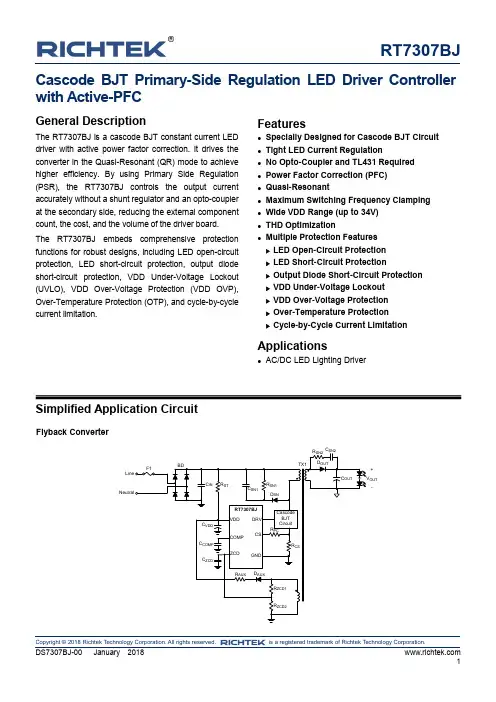
RT7307BJCopyright © 2018 Richtek Technology Corporation. All rights reserved. is a registered trademark of Richtek Technology Corporation.DS7307BJ-00 January 20181Cascode BJT Primary-Side Regulation LED Driver Controller with Active-PFCGeneral DescriptionThe RT7307BJ is a cascode BJT constant current LED driver with active power factor correction. It drives the converter in the Quasi-Resonant (QR) mode to achieve higher efficiency. By using Primary Side Regulation (PSR), the RT7307BJ controls the output current accurately without a shunt regulator and an opto-coupler at the secondary side, reducing the external component count, the cost, and the volume of the driver board. The RT7307BJ embeds comprehensive protection functions for robust designs, including LED open-circuit protection, LED short-circuit protection, output diode short-circuit protection, VDD Under-Voltage Lockout (UVLO), VDD Over-Voltage Protection (VDD OVP), Over-Temperature Protection (OTP), and cycle-by-cycle current limitation.Features● Specially Designed for Cascode BJT Circuit ● Tight LED Current Regulation ● No Opto-Coupler and TL431 Required ● Power Factor Correction (PFC) ● Quasi-Resonant● Maximum Switching Frequency Clamping ● Wide VDD Range (up to 34V) ● THD Optimization●Multiple Protection Features④ LED Open-Circuit Protection ④ LED Short-Circuit Protection④ Output Diode Short-Circuit Protection ④ VDD Under-Voltage Lockout ④ VDD Over-Voltage Protection ④ Over-Temperature Protection④ Cycle-by-Cycle Current LimitationApplications●AC/DC LED Lighting DriverSimplified Application CircuitFlyback Converter+OUT-RT7307BJCopyright © 2018 Richtek Technology Corporation. All rights reserved. is a registered trademark of Richtek Technology Corporation. DS7307BJ-00 January 20182Ordering InformationRT7307BJG : Green (Halogen Free and Pb Free)Note :Richtek products are :④ RoHScompliant and compatible with the currentrequirements of IPC/JEDEC J-STD-020.④ Suitable for use in SnPb or Pb-free soldering processes.Marking Information5H= : Product Code DNN : Date CodePin Configuration(TOP VIEW)SOT-23-6RT7307BJCopyright © 2018 Richtek Technology Corporation. All rights reserved. is a registered trademark of Richtek Technology Corporation.DS7307BJ-00 January 20183Functional Block DiagramDRVGNDVDDOperationCritical-Conduction Mode (CRM) with Constant On-Time ControlFigure 1 shows a typical flyback converter with input voltage (V IN ). When main switch Q1 is turned on with a fixed on-time (t ON ), the peak current (I L_PK ) of the magnetic inductor (L m ) can be calculated by the following equation : IN L_PK ON mVI t L =⨯TX1OUTV OUTFigure 1. Typical Flyback ConverterIf the input voltage is the output voltage of the full-bridge rectifier with sinusoidal input voltage (V IN_PK ⋅sin(θ)), the inductor peak current (I L_PK ) can be expressed as the following equation :IN_PK ONL_PK mV sin(θ)t I L ⨯⨯=When the converter operates in CRM with constant on-time control, the envelope of the peak inductor current will follow the input voltage waveform with in-phase. Thus, high power factor can be achieved, as shown in Figure 2.RT7307BJCopyright © 2018 Richtek Technology Corporation. All rights reserved. is a registered trademark of Richtek Technology Corporation. DS7307BJ-00 January 20184I L_PK I Q1I in_avg I Do Peak Inductor Current Switch Current Average Input Current Output Diode Current V IN Input Voltage DRVDriving signalFigure 2. Inductor Current of CRM with ConstantOn-Time ControlThe RT7307BJ needs no shunt regulator and opto-coupler at the secondary side to achieve the output current regulation. Figure 3 shows several key waveforms of a conventional flyback converter in Quasi-Resonant (QR) mode, in which V AUX is the voltage on the auxiliary winding of the transformer.VV I I V Figure 3. Key Waveforms of a Flyback ConverterVoltage Clamping CircuitThe RT7307BJ provides a voltage clamping circuit at ZCD pin since the voltage on the auxiliary winding is negative when the main switch is turned on. The lowest voltage on ZCD pin is clamped near zero to prevent the IC from being damaged by the negative voltage. Meanwhile, the sourcing ZCD current (I ZCD ), flowing through the upper resistor (R ZCD1), is sampled and held to be a line-voltage-related signal for propagation delay compensation. The RT7307BJ embeds the programmablepropagation delay compensationthrough CS pin. A sourcing current I CS (equal to I ZCD x K PC ) applies a voltage offset (I CS x R PC ) which is proportional to line voltage on CS to compensate the propagation delay effect. Thus, the output current can be equal at high and low line voltage.Quasi-Resonant OperationFigure 4 illustrates how valley signal triggers PWM. If no valley signal detected for a long time, the next PWM is triggered by a starter circuit at end of the interval (t START , 130μs typ.) which starts at the rising edge of the previous PWM signal. A blanking time (t S(MIN), 8.5μs typ.), which starts at the rising edge of the previous PWM signal, limits minimum switching period. When the t S(MIN) interval is on-going, all of valley signals are not allowed to trigger the next PWM signal.After the end of the t S(MIN) interval, the coming valley will trigger the next PWM signal. If one or more valley signals are detected during the t S(MIN) interval and no valley is detected after the end of the t S(MIN) interval, the next PWM signal will be triggered automatically at end of the t S(MIN) + 5μs (typ.).RT7307BJCopyright © 2018 Richtek Technology Corporation. All rights reserved. is a registered trademark of Richtek Technology Corporation.DS7307BJ-00 January 20185PWMValley Signal PWMValley Signal PWMValley Signal PWMValley SignalFigure 4. PWM Triggered MethodProtectionsLED Open-Circuit ProtectionIn an event of output open circuit, the converter will be shut down to prevent being damaged, and it will be auto-restarted when the output is recovered. Once the LED is open-circuit, the output voltage keeps rising, causing the voltage on ZCD pin V ZCD rising accordingly. When the sample-and-hold ZCD voltage (V ZCD_SH )exceeds its OV threshold (V ZCD_OVP , 3.2V typ.), output OVP will be activated and the PWM output (DRV pin) will be forced low to turn off the main switch. If the output is still open-circuit when the converter restarts, the converter will be shut down again. Output Diode Short-Circuit ProtectionWhen the output diode is damaged as short-circuit, the transformer will be led to magnetic saturation and the main switch will suffer from a high current stress. To avoid the above situation, an output diode short-circuit protection is built-in. When CS voltage V CS exceedsthe threshold (V CS_SD 1.7 typ.) of the output diode short-circuit protection, the RT7307BJ will shut down the PWM output (DRV pin) in few cycles to prevent the converter from damage. It will be auto-restarted when the failure condition is recovered.VDD Under-Voltage Lockout (UVLO) and Over-Voltage Protection (VDD OVP)The RT7307BJ will be enabled when VDD voltage (V DD ) exceeds rising UVLO threshold (V TH_ON , 17V typ.) and disabled when V DD is lower than falling UVLO threshold (V TH_OFF , 8.5V typ.).When V DD exceeds its over-voltage threshold (V OVP , 37.4V typ.), the PWM output of the RT7307BJ is shut down. It will be auto-restarted when the VDD is recovered to a normal level.Over-Temperature Protection (OTP)The RT7307BJ provides an internal OTP function to protect the controller itself from suffering thermal stressand permanent damage. It's not suggested to use the function as precise control of over temperature. Once the junction temperature is higher than the OTP threshold (T OTP , 150︒C typ.), the controller will shut down until the temperature cools down by 30︒C (typ.). Meanwhile, if V DD reaches falling UVLO threshold voltage (V TH_OFF ), the controller will hiccup till the over temperature condition is removed.RT7307BJCopyright © 2018 Richtek Technology Corporation. All rights reserved. is a registered trademark of Richtek Technology Corporation. DS7307BJ-00 January 20186Absolute Maximum Ratings (Note 1)● Supply Voltage, V DD -------------------------------------------------------------------------------------------------- -0.3V to 40V ● Driver Output, DRV --------------------------------------------------------------------------------------------------- -0.3V to 20V ● Other Pins --------------------------------------------------------------------------------------------------------------- -0.3V to 6V ●Power Dissipation, P D @ T A = 25︒CSOT-23-6 ---------------------------------------------------------------------------------------------------------------- 0.42W ●Package Thermal Resistance (Note 2)SOT-23-6, θJA ---------------------------------------------------------------------------------------------------------- 235.6︒C/W● Lead Temperature (Soldering, 10 sec.) -------------------------------------------------------------------------- 260︒C ● Junction Temperature ------------------------------------------------------------------------------------------------ 150︒C● Storage Temperature Range --------------------------------------------------------------------------------------- -65︒C to 150︒C ●ESD Susceptibility (Note 3)HBM (Human Body Model) ----------------------------------------------------------------------------------------- 2kVRecommended Operating Conditions (Note 4)● Supply Input Voltage, V DD ----------------------------------------------------------------------------------------- 11V to 34V ● COMP Voltage, V COMP ---------------------------------------------------------------------------------------------- 0.7V to 4.3V ●Junction Temperature Range -------------------------------------------------------------------------------------- -40︒C to 125︒CElectrical Characteristics(V= 15V, T = 25︒C, unless otherwise specified)RT7307BJCopyright © 2018 Richtek Technology Corporation. All rights reserved. is a registered trademark of Richtek Technology Corporation.DS7307BJ-00 January 20187Note 1. Stresses beyond those listed “Absolute Maximum Ratings” may cause permanent damage to the device. These arestress ratings only, and functional operation of the device at these or any other conditions beyond those indicated in the operational sections of the specifications is not implied. Exposure to absolute maximum rating conditions may affect device reliability. Note 2. θJA is measured under natural convection (still air) at T A = 25︒C with the component mounted on a loweffective-thermal-conductivity two-layer test board on a JEDEC thermal measurement standard. Note 3. Devices are ESD sensitive. Handling precaution recommended. Note 4. The device is not guaranteed to function outside its operating conditions. Note 5. Guarantee by design.RT7307BJCopyright © 2018 Richtek Technology Corporation. All rights reserved. is a registered trademark of Richtek Technology Corporation. DS7307BJ-00 January 20188Typical Application CircuitFlyback Converter+OUT-RT7307BJCopyright © 2018 Richtek Technology Corporation. All rights reserved. is a registered trademark of Richtek Technology Corporation.DS7307BJ-00 January 20189Typical Operating CharacteristicsV OVP vs. Junction Temperature36.036.136.236.336.436.536.636.7-50-25255075100125Junction Temperature (°C)V O V P (V)V TH_OFF vs. Junction Temperature8.408.448.488.528.568.60-50-25255075100125Junction Temperature (°C)V T H _O F F (V)I DD_OP vs. Junction Temperature1.651.701.751.801.851.901.952.00-50-25255075100125Junction Temperature (°C)I D D _O P (m A)K CC vs. Junction Temperature252254256258260-50-25255075100125Junction Temperature (°C)K C C (m V)V CS_SD vs. Junction Temperature1.7501.7751.8001.8251.850-50-25255075100125Junction Temperature (°C)V C S _S D (V)V CS_CL vs. Junction Temperature1.181.201.221.241.261.281.30-50-25255075100125Junction Temperature (°C)V C S _C L (V )RT7307BJCopyright © 2018 Richtek Technology Corporation. All rights reserved. is a registered trademark of Richtek Technology Corporation. DS7307BJ-00 January 201810K PC vs. Junction Temperature0.0400.0410.0420.0430.0440.045-50-25255075100125Junction Temperature (°C)K P C (A /A)t START vs. Junction Temperature90100110120130140150-50-25255075100125Junction Temperature (°C)t S T A R T (μs )Application InformationOutput Current SettingConsidering the conversion efficiency, the programmed DC level of the average output current (I OUT (t)) can be derived as :P CC OUT_CC TX1S CS1N K I CTR 2N R =⨯⨯⨯SEC_PK STX1PRI_PK PI N CTR I N =⨯in which CTR TX1 is the current transfer ratio of the transformer TX1, I SEC_PK is the peak current of the secondary side, and I PRI_PK is the peak current of the primary side. CTR TX1 can be estimated to be 0.9. According to the above parameters, current sense resistor R CS can be determined as the following equation :P CC CS TX1S OUT_CC1N K R CTR 2N I =⨯⨯⨯Propagation Delay Compensation DesignThe V CS deviation (∆V CS ) caused by propagation delay effect can be derived as: IN D CS CS mV t RV L ⋅⋅∆=,in which t D is the delay period which includes the propagation delay of the RT7307BJ and the turn-off transition of the main switch. The sourcing current from CS pin of the RT7307BJ (I CS ) can be expressed as : A CS PC IN P ZCD1N1I K V N R =⋅⋅⋅where N A is the turns number of the auxiliary winding. R PC can be designed by : CS D CS ZCD1PPC CS m PC AV t R R N R I L K N ∆⋅⋅==⋅⋅ Output Over-Voltage Protection SettingOutput OVP is achieved by sensing the voltage on the auxiliary winging. It is recommended that output OV level (V OUT_OVP ) is set at 120% of nominal output voltage (V OUT ). Thus, R ZCD1 and R ZCD2 can be determined by the equation as :ZCD2A OUT S ZCD1ZCD2R NV 120% 3.2V(typ.)N R R ⨯⨯⨯=+Thermal ConsiderationsFor continuous operation, do not exceed absolute maximum junction temperature. The maximum power dissipation depends on the thermal resistance of the IC package, PCB layout, rate of surrounding airflow, and difference between junction and ambient temperature. The maximum power dissipation can be calculated by the following formula : P D(MAX) = (T J(MAX) − T A ) / θJAWhere T J(MAX) is the maximum junction temperature, T A is the ambient temperature, and θJA is the junction to ambient thermal resistance.For recommended operating condition specifications, the maximum junction temperature is 125°C. The junction to ambient thermal resistance, θJA , is layout dependent. For SOT-23-6 packages, the thermal resistance, θJA , is 235.6°C/W on a standard JEDEC 51-3 two-layer thermal test board. The maximum power dissipation at T A = 25°C can be calculated by the following formula:P D(MAX) = (125°C − 25°C) / (235.6°C/W) = 0.42W for a SOT-23-6 package.The maximum power dissipation depends on the operating ambient temperature for fixed T J(MAX) and thermal resistance, θJA . The derating curve in Figure 5 allows the designer to see the effect of rising ambient temperature on the maximum power dissipation.Figure 5. Derating Curve of Maximum PowerDissipationLayout ConsiderationsA proper PCB layout can abate unknown noise interference and EMI issue in the switching power supply. Please refer to the guidelines when designing a PCB layout for switching power supply :④The current path(1) from input capacitor, transformer, switch, R CS return to input capacitor is a high frequency current loop. The path(2) from DRV pin, switch, R CS return to the ground of the IC is also a high frequency current loop. They must be as short as possible to decrease noise coupling and kept a space to other low voltage traces, such as IC control circuit paths, especially. Besides, the path(3) between switch ground(b) and IC ground(d) is recommended to be as short as possible, too.④The path(4) from RCD snubber circuit to switch is a high switching loop. Keep it as small as possible. ④It is good for reducing noise, output ripple and EMI issue to separate ground traces of input capacitor(a), switch(b), auxiliary winding(c) and IC control circuit(d). Finally, connect them together on input capacitor ground(a). The areas of these ground traces should be kept large.④To minimize parasitic trace inductance and EMI, minimize the area of the loop connecting the secondary winding, the output diode, and the output filter capacitor. In addition, apply sufficient copper area at the anode and cathode terminal of the diode for heat-sinking. It is recommended to apply a larger area at the quiet cathode terminal. A large anode area will induce high-frequency radiated EMI.0.00.10.20.30.40.50.6255075100125Ambient Temperature (°C)M a x i m u m P o w e r D i s s i p a t i o n (W )Figure 6. PCB Layout GuideOutline DimensionSOT-23-6 Surface Mount PackageFootprint InformationRichtek Technology Corporation14F, No. 8, Tai Yuen 1st Street, Chupei CityHsinchu, Taiwan, R.O.C.Tel: (8863)5526789Richtek products are sold by description only. Richtek reserves the right to change the circuitry and/or specifications without notice at any time. Customers should obtain the latest relevant information and data sheets before placing orders and should verify that such information is current and complete. Richtek cannot assume responsibility for use of any circuitry other than circuitry entirely embodied in a Richtek product. Information furnished by Richtek is believed to be accurate and reliable. However, no responsibility is assumed by Richtek or its subsidiaries for its use; nor for any infringements of patents or other rights of third parties which may result from its use. No license is granted by implication or otherwise under any patent or patent rights of Richtek or its subsidiaries.。

---------------------------------------------------------------最新资料推荐------------------------------------------------------中英文对照术语表A Absorption costing（完全成本法）Accelerated depreciation method（加速折旧法） Account（账户） Account form （账户式） Account payable（应付账款） Account receivable （应收账款） Accounting（会计） Accounting cycle（会计循环）Accounting equation（会计恒等式） Accounting period concept （会计期间概念） Accounting system（会计系统） Accounts payable subsidiary ledger（应付账款明细分类账）（应付账款明细分类账） Accounts receivable subsidiary ledger（应收账款明细分类账）（应收账款明细分类账） Accounts receivable turnover （应收账款周转率） Accrual basis（应计制；权责发生制）Accruals（应计项目） Accrued assets（应计资产） Accrued expenses（应计费用） Accrued liabilities（应计负债） Accrued revenues（应计收入） Accumulated depreciation（累计折旧）Accumulated other comprehensive income（累计其他全面收益）（累计其他全面收益） Activity base (driver)（作业基础/动因）Activity-based costing (ABC)（作业成本计算法） Adjusted trial balance（调整后试算平衡表） Adjusting entries（调整分录）Adjusting process（调整过程）Administrative expenses (general expenses)（管理费用（一般费用））Aging the receivables（应收账款账龄分析） Allowance method（备抵法）1/ 12Amortization（摊销）Annuity（年金）Assets（资产）Available-for-sale securities（可供出售证券） Average cost method（平均成本法） Average rate of return（平均回报率） B Balance of the account（账户余额） Balance sheet（资产负债表） Balanced scorecard（平衡记分卡） Bank reconciliation （银行存款余额调节表） Bond（债券） Bond indenture（债券契约） Book value（账面价值） Book value of the asset（资产的账面价值） Boot（补价） Bottleneck（瓶颈） Break-even point （盈亏临界点） Budget（预算） Budget performance report（预算业绩报告） Budgetary slack（预算松弛） Business（企业）Business entity concept（企业主体概念） Business stakeholder （企业利益相关者） Business strategy（企业战略） Business transaction（经济业务） C Capital expenditures（资本性支出） Capital expenditures budget（资本支出预算） Capital investment analysis（资本投资分析）Capital leases（资本性租赁） Capital rationing（资本分配）Carrying amount（账面金额） Cash（现金） Cash basis（现金制；收付实现制） Cash budget（现金预算） Cash dividend（现金股利） Cash equivalents（现金等价物） Cash flows from financing activities（筹资活动现金流量）（筹资活动现金流量）Cash flows from investing activities（投资活动现金流量）（投资活动现金流量） Cash flows from operating activities（经营---------------------------------------------------------------最新资料推荐------------------------------------------------------ 活动现金流量）（经营活动现金流量） Cash payback period（现金回收期） Cash payments journal（现金付款日记账） Cash receipts journal（现金收款日记账） Cash short and over account （现金余缺账户） Certified public accountant (CPA)（注册会计师） Chart of accounts（会计科目表） Clearing account(清理账户) Closing entries（结账分录） Closing process（结账程序） Combination strategy（混合战略） Common stock（普通股）Common-size statement（通用报表） Component（成分；组成部分）Comprehensive income（全面收益）Consolidated financial statements（合并财务报表）（合并财务报表） Consolidation（创立合并） Continuous budgeting（滚动预算） Contra account （抵减账户） Contract rate（约定利率） Contribution margin(贡献毛益) Contribution margin ratio（贡献毛益率） Controllable expenses（可控费用）Controllable variance（可控差异）Controller（主计长）Controlling account（控制账户）Conversion costs（加工成本） Copyright（版权） Corporation （公司） Cost（成本） Cost accounting system（成本会计系统）Cost allocation（成本分配） Cost behavior（成本性态） Cost center（成本中心） Cost of goods sold（产品销售成本） Cost of goods sold budget（产品销售成本预算） Cost of merchandise sold（商品销售成本） Cost of production report（生产成本报3/ 12告） Cost per equivalent unit（单位约当产量成本） Cost price approach（成本价格法）Cost variance（成本差异）Cost-volume-profit analysis（本－量－利分析）Cost-volume-profit chart（本－量－利图） Credit memorandum （贷项通知单） Credits（贷记） Cumulative preferred stock （累积优先股） Currency exchange rate（货币汇率） Current assets（流动资产） Current liabilities（流动负债） Current ratio（流动比率） Currently attainable standards（当前可达标准） D Debit memorandum（借项通知单）Debits（借记） Decentralization（分权） Declining-balance method（余额递减法） Deferred expenses（递延费用） Deferred revenues（递延收入） Deficiency（亏损） Deficit（亏损）Defined benefit plan（固定收益计划） Defined contribution plan （固定缴款计划） Depletion（折耗） Depreciation（折旧）Depreciation expense（折旧费用） Differential analysis（差异分析） Differential cost（差异成本） Differential revenue （差异收入） Differential strategy（差异化战略） Direct labor cost（直接人工成本） Direct labor rate variance（直接人工工资率差异） Direct labor time variance（直接人工工时差异）Direct materials cost（直接材料成本） Direct materials price variance（直接材料价格差异）（直接材料价格差异） Direct materials purchases budget（直接材料采购预算）（直接材料采购---------------------------------------------------------------最新资料推荐------------------------------------------------------ 预算） Direct materials quantity variance（直接材料数量差异）（直接材料数量差异） Direct method（直接法） Direct write-off method（直接注销法） Discontinued operations（停止经营）Discount（贴现息；折价） Discount rate（贴现率） Dishonored note receivable（拒付应收票据） Dividend yield（股利收益率）Division（分部） Doomsday ration（终极流动比率） Double-entry accounting（复式会计） Drawing（提款） DuPont formula（杜邦公式） E Earnings per common share (EPS)（每股收益）Earnings per common share (EPS) on common stock（普通股每股收益） E-commerce（电子商务） Effective interest rate method （实际利率法）Effective rate of interest（实际利率）Electronic funds transfer (EFT)（电子资金转账） Elements of internal control（内部控制要素） Employee fraud（员工舞弊）Employee s earnings record（员工收入记录） Equity method（权益法） Equity securities（权益证券） Equivalent units of production（约当产量） Ethics（伦理） Expenses（费用）Extraordinary items（非常项目） F Factory overhead cost（制造费用） FICA tax（联邦社会保险税） Financial accounting （财务会计） Financial Accounting Standards Board (FASB)（财务会计准则委员会） Financial statements（财务报表） Finished goods inventory（完工产品存货） Finished goods ledger（完工5/ 12产品分类账） First-in, first-out (fifo) method（先进先出法）Fiscal year（会计年度） Fixed (plant) assets（固定资产） Fixed asset impairment（固定资产减值） Fixed assets（固定资产）Fixed costs（固定成本） Flexible budget（弹性预算） FOB (free on board) destination（目的地交货） FOB (free on board) shipping point（装运地交货）（装运地交货） Free cash flow（自由现金流量） Fringe benefits（额外福利） Future value（未来价值，终值） G General journal（普通日记账） General ledger（总分类账） Generally accepted accounting principles (GAAP)（公认会计原则） Goal conflict（目标冲突） Goodwill （商誉） Gross pay（工资总额） Gross profit（毛利） Gross profit method（毛利法） H Held-to-maturity securities（持有至到期证券） High-low method（高低点法） Horizontal analysis （水平分析） I Ideal standards（理想标准） Income from operations (operating income) （营业利润）（营业利润） Income statement（损益表） Income summary（收益汇总） Indirect method （间接法） Inflation（通货膨胀） Initial public offering (IPO)（首次公开招股） Intangible assets（无形资产） Internal controls（内部控制） Internal rate of return method（内含回报率法） Inventory shrinkage（存货损耗） Inventory turnover （存货周转率） Investment center（投资中心） Investment turnover（投资周转率） Investments（投资） Invoice（发票）---------------------------------------------------------------最新资料推荐------------------------------------------------------J Job cost sheet（分批成本计算单） Job order cost system（分批成本计算法） Journal（日记账） Journal entry（日记账分录）Journalizing（编制分录） Just-in-time (JIT) processing（适时加工制） L Last-in, first-out (lifo) method（后进先出法）Ledger（分类账） Leverage（杠杆收益） Liabilities（负债）Limited liability corporation (LLC)（有限责任公司）（有限责任公司） Liquidation（清算） Long-term liabilities（长期负债）Low-cost strategy（低成本战略） Lower-of-cost-or-market (LCM) method（成本与市价孰低法）（成本与市价孰低法） M Management Discussion and Analysis (MDA)（管理层讨论与分析） Managerial accounting（管理会计） Manufacturing business（制造企业）Manufacturing cells（制造单元） Margin of safety（安全边际）Market price approach（市场价格法） Markup（加成） Master budget（全面预算） Matching concept（配比概念） Materiality concept（重要性概念）Materials inventory（材料存货）Materials ledger（材料分类账） Materials requisitions（领料单） Maturity value（到期值） Merchandise inventory（商品存货） Merchandising business（商业企业） Merger（吸收合并）Minority interest（少数股权）Mixed cost（混合成本）Multiple-step income statement （多步式损益表） N Natural business year（自然营业年度） Negotiated price approach（协7/ 12议价格法） Net income（净利润） Net loss（净亏损） Net pay （工资净额） Net present value method（净现值法） Net realizable value（可变现净值） Nonparticipation preferred stock（非参与优先股）（非参与优先股） Note receivable（应收票据） Number of days sales in inventory（存货销售周期）（存货销售周期） Number of days sales in receivables（应收账款周转天数）（应收账款周转天数） Number of times interest charges are earned(利息保障倍数) O Operating leases（经营性租赁）Operating leverage（经营杠杆） Opportunity cost（机会成本）Other comprehensive income（其他全面收益） Other expense（其他费用） Other income（其它收入） Outstanding stock（流通在外股票） Overapplied factory overhead（制造费用过度分配）（制造费用过度分配） Owners equity（所有者权益） P Paid-in capital（实缴资本） Par（面值） Parent company（母公司）Partnership（合伙企业） Partnership agreement（合伙契约）Patents（专利权） Payroll（工资） Payroll register（工资表）Period costs（期间成本） Periodic method（定期盘存制）Permanent differences（永久性差异） Perpetual method（永续盘存制） Petty cash fund（备用金） Physical inventory（实地盘存） Post-closing trial balance（结账后试算平衡表）Posting（过账） Predetermined factory overhead rate（预定制造费用分配率）（预定制造费用分配率） Preferred stock（优先股）---------------------------------------------------------------最新资料推荐------------------------------------------------------ Premium（溢价） Prepaid expenses（预付费用） Present value （现值） Present value concept（现值概念） Present value index（现值指数） Present value of an annuity（年金现值）Price-earnings (P/E) ratio（市盈率） Price-earnings ratio （市盈率） Prior period adjustments（前期调整） Private accounting（内部会计） Proceeds（贴现净额） Process（流程；步骤）Process cost system（分步成本计算法）Process manufacturers（分步制造企业） Product cost concept（产品成本概念） Product costs（产品成本） Production budget（生产预算） Profit center（利润中心） Profit margin（销售利润率）Profitability（获利能力） Profit-volume chart（利润－产量图）Promissory note（承兑票据） Property, plant, and equipment （财产、厂房和设备）（财产、厂房和设备） Proprietorship(独资企业) Public accounting（公共会计） Purchase method(购买法) Purchase return or allowance（购货退回或折让） Purchases discounts（购货折扣） Purchases journal（采购日记账） Q Quick assets（速动资产） Quick ratio（速动比率） R Rate earned on common stockholders equity（普通股股东权益收益率） Rate earned on stockholders equity（股东权益收益率）（股东权益收益率） Rate earned on total assets（总资产收益率） Rate of return on investment (ROI)（投资回报率）（投资回报率） Ratio of fixed9/ 12assets to long-term liabilities（固定资产对长期负债比率）（固定资产对长期负债比率） Ratio of liabilities to stockholders equity（负债对股东权益比率）（负债对股东权益比率） Real accounts（实账户） Realization（变现） Receivables（应收款项） Receiving report（收货单） Relevant range（相关范围）Report form（报告式） Residual income（剩余收益） Residual value（残值）Responsibility accounting（责任会计）Responsibility center（责任中心）Restrictions（限制）Restructuring charge（重组费用） Retail inventory method（零售价格法） Retained earnings（留存收益） Retained earnings statement（留存收益表） Revenue expenditure（收益性支出）Revenue journal（收入日记账） Revenue recognition concept （收入确认概念） Revenues（收入） Reversing entry（转回分录） S Sales（销售收入） Sales budget（销售预算） Sales discounts（销售折扣） Sales mix（销售组合） Sales returns and allowances（销售退回与折让） Selling expenses（销售费用）Service business（服务企业） Service department charges（服务部门费用） Single-step income statement（单步式损益表）Sinking fund（偿债基金） Slide（滑位） Solvency（偿债能力）Special journals（专用日记账） Standard cost（标准成本）Standard cost systems（标准成本系统） Stated value（设定价值） Statement of cash flows（现金流量表） Statement of---------------------------------------------------------------最新资料推荐------------------------------------------------------ members equity（成员权益报表） Statement of owner s equity （所有者权益表） Statement of partnership equity（合伙企业权益表）（合伙企业权益表）Statement of partnership liquidation（合伙企业清算表）（合伙企业清算表） Statement of stockholders equity（股东权益表） Static budget（固定预算）Stock（股票） Stock dividend（股票股利） Stock split（股票分割） Stockholders（股东） Stockholders equity（股东权益）Straight-line method（直线法） Subsidiary company（子公司）Sunk cost(沉没成本) T T account（T 型账户） Target costing （目标成本法） Taxable income（应税所得） Temporary (nominal) accounts（临时性（虚）账户）（临时性（虚）账户） Temporary differences（暂时性差异） Temporary investments（临时性投资）Theory of constraints (TOC)（限制理论） Time tickets（计工单） Time value of money concept（货币时间价值概念）（货币时间价值概念） Total cost concept（完全成本概念） Trade discounts（商业折扣） Trade-in allowance（以旧换新折让）Trademark（商标） Trading securities（交易证券） Transfer price（转移价格） Transposition（换位） Treasury stock（库藏股票） Trial balance（试算平衡） Two-column journal（两栏式日记账） U Uncollectible accounts expense（坏账费用）Underapplied factory overhead（制造费用分配不足）（制造费用分11/ 12配不足） Underwriting firms（证券包销公司） Unearned revenue （预收收入） Unearned revenues（预收收入） Unit contribution margin（单位贡献毛益） Unit of measure concept（计量单位概念） Units-of-production method（产量法） Unrealized holding gain or loss（未实现持有利得或损失） V Value chain（价值链）Variable cost concept（变动成本概念） Variable costing（变动成本计算） Variable costs（变动成本） Venture capitalist (VC)（风险投资家） Vertical analysis（垂直分析） Volume variance（产量差异） Voucher（付款凭单） Voucher system（付款凭单制度） Work in process inventory（在产品存货） Work sheet（工作底稿） Working capital（营运资本） Yield（收益率） Zero-based budgeting（零基预算）。

这个驱动程序包含了三个函数：DriverEntry、HelloDDKUnload和HelloDDKDispatchRoutine。

其中DriverEntry是驱动程序的入口函数，相当于C/C++程序的main函数，HelloDDKUnload函数是驱动卸载函数。

而HelloDDKDispatchRuntine则是IRP的派遣函数，因为驱动程序主要是处理IO 请求，而IO请求大多是在派遣函数中处理的。

先来看看这个驱动程序的第一个函数：DriverEntry/***************************************************************** 函数名称：DriverEntry* 功能描述：初始化驱动程序，定位和申请硬件资源，创建内核对象* 参数列表：pDriverObject:从I/O管理器中传来的驱动对象pRegistryPath:驱动程序在注册表中的路径* 返回值：返回初始化驱动状态****************************************************************/#pragma INITCODEextern "C" NTSTATUS DriverEntry( IN PDRIVER_OBJECT pDriverObject,IN PUNICODE_STRING pRegistryPath ){NTSTATUS status;KdPrint( ( "Enter DriverEntry!\n" ) );//注册其它驱动调用函数入口pDriverObject->DriverUnload = ( PDRIVER_UNLOAD ) HelloDDKUnload; pDriverObject->MajorFunction[IRP_MJ_CREATE] = HelloDDKDispatchRoutine; pDriverObject->MajorFunction[IRP_MJ_CLOSE] = HelloDDKDispatchRoutine; pDriverObject->MajorFunction[IRP_MJ_WRITE] = HelloDDKDispatchRoutine; pDriverObject->MajorFunction[IRP_MJ_READ] = HelloDDKDispatchRoutine;//创建驱动设备对象status = CreateDeivce( pDriverObject );KdPrint( ( "DriverEntry end!\n" ) );return status;}这个函数的第一句代码是一个#pragma预处理指令：#pragma INITCODE这段代码表明将此函数加入INIT内存区域。